Financial Optimization ISE 347/447 Lecture 13ted/files/ie447/lectures/Lecture13.pdfISE 347/447...

Financial OptimizationISE 347/447

Lecture 13

Dr. Ted Ralphs

ISE 347/447 Lecture 13 1

Reading for This Lecture

• C&T Chapter 11

1


Integer Linear Optimization

• An integer linear optimization problem (ILP) is the same as a linearoptimization problem except that the variables can take on only integervalues.

• If only some of the variables are constrained to take on integer values,then we call the program a mixed integer linear optimization problem(MILP).

• The general form of an MILP is

min c>x+ d>y

s.t. Ax+By = b

x, y ≥ 0

x ∈ Zp × Rn−p

2


Mixed Integer Nonlinear Optimization Problem

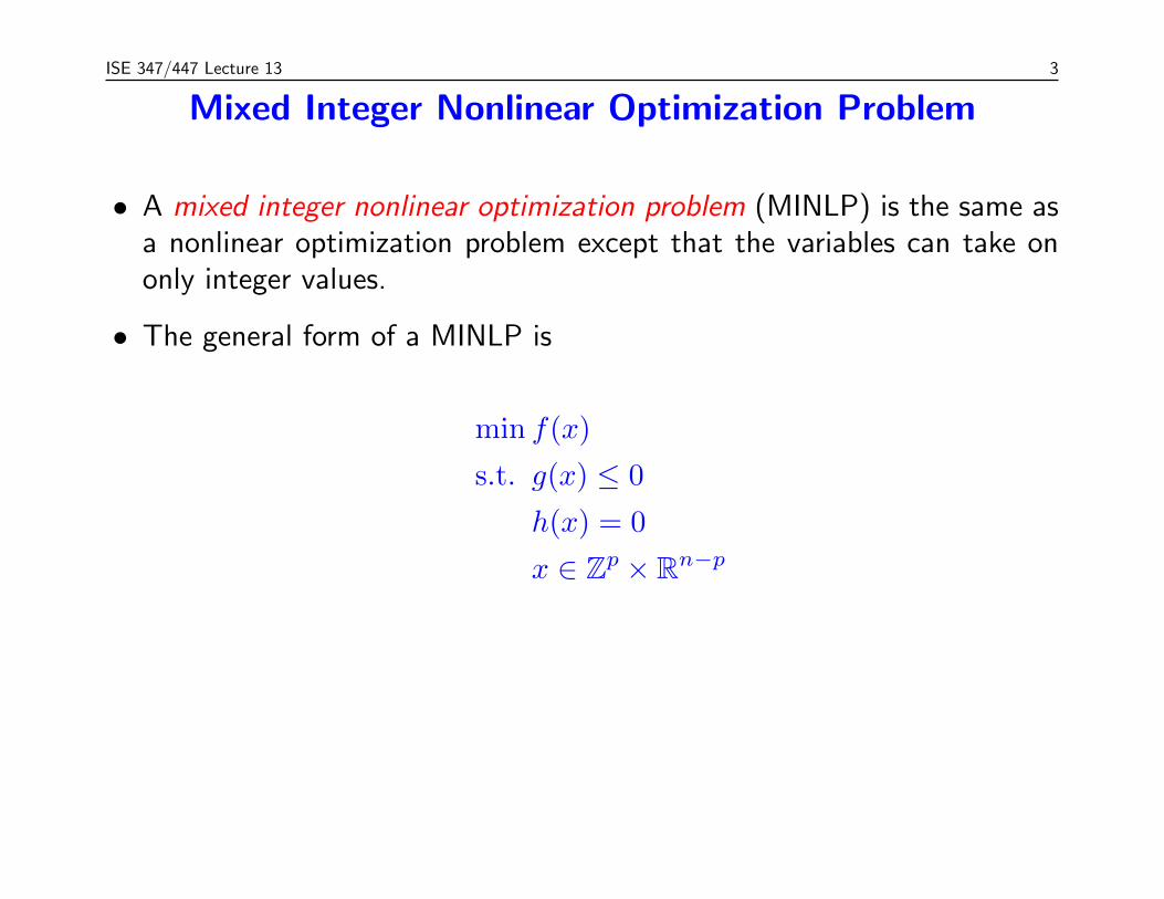
• A mixed integer nonlinear optimization problem (MINLP) is the same asa nonlinear optimization problem except that the variables can take ononly integer values.

• The general form of a MINLP is

min f(x)

s.t. g(x) ≤ 0

h(x) = 0

x ∈ Zp × Rn−p

3


Modeling with Integer Variables

• Why do we need integer variables?

• If the variable is associated with a physical entity that is indivisible, thenit must be integer.

– Shares of a stock.– Investments that can only be made in fixed amounts.

• 0-1 (binary) variables can be used to model logical conditions orcombinatorial structure.

– Modeling yes/no decisions.– Enforcing disjunctions.– Enforcing logical constraints.– Modeling fixed costs.– Modeling piecewise linear functions.

4


Conjunction versus Disjunction

• A more general mathematical view that ties integer programming to logicis to think of integer variables as expressing disjunction.

• The constraints of a standard mathematical program are conjunctive.

– All constraints must be satisfied.– In terms of logic, we have

g1(x) ≤ b1 AND g2(x) ≤ b2 AND · · · AND gm(x) ≤ bm (1)

– This corresponds to intersection of the regions associated with eachconstraint.

• Integer variables introduce the possibility to model disjunction.

– At least one constraint must be satisfied.– In terms of logic, we have

g1(x) ≤ b1 OR g2(x) ≤ b2 OR · · · OR gm(x) ≤ bm (2)

– This corresponds to union of the regions associated with eachconstraint.

5


How Hard is Integer Programming?

• Solving general integer programs can be much more difficult than solvinglinear programs.

• There is no known polynomial-time algorithm for solving general MILPs.

• Solving the associated linear programming relaxation provides a lowerbound on the optimal solution value of a given MILP.

• In general, an optimal solution to the LP relaxation may not tell us muchabout an optimal solution to the MILP.

– Rounding to a feasible integer solution may be difficult.– The optimal solution to the LP relaxation can be arbitrarily far away

from the optimal solution to the MILP.– Rounding may result in a solution far from optimal.– We can sometimes bound the difference between the optimal solution

to the LP and the optimal solution to the MILP (how?).

6


The Geometry of Integer Programming

• Let’s consider again an integer linear program

min c>x

s.t. Ax = b

x ≥ 0

x integer

• The feasible region is the integer points inside a polyhedron.

• It is not difficult to see why solving the LP relaxation does not necessarilyyield a solution near an integer optimum.

7


Easy Integer Programs

• Certain integer programs are “easy”.

• What makes an integer program “easy”?

– All of the extreme points of the LP relaxation are integral.– Every square submatrix of A has determinant +1, -1, or 0.– We know a complete description of the convex hull of feasible solutions.– We have an efficient algorithm for finding an optimal integer solution

(not based on linear programming).– There is no duality gap (more on this later).

• Examples of “easy” integer programs.

– Minimum cost network flow problem.– Maximum flow problem.– Assignment problem.

8


Modeling Binary Choice

• We use binary variables to model yes/no decisions.

• Example: Integer knapsack problem

– We are given a set of items with associated values and weights.– We wish to select a subset of maximum value such that the total

weight is less than a constant K.– We associate a 0-1 variable with each item indicating whether it is

selected or not.

max

m∑j=1

cjxj

s.t.

m∑j=1

wjxj ≤K

x≥ 0

x integer

• Knapsack problems arise as subproblems in many financial applications.

9


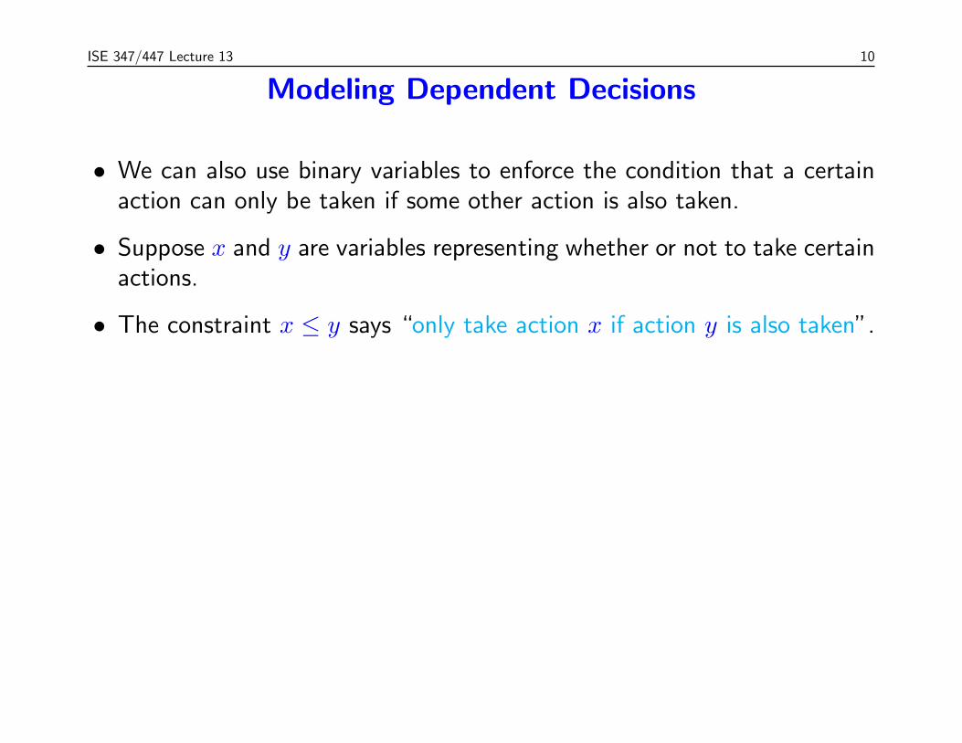
Modeling Dependent Decisions

• We can also use binary variables to enforce the condition that a certainaction can only be taken if some other action is also taken.

• Suppose x and y are variables representing whether or not to take certainactions.

• The constraint x ≤ y says “only take action x if action y is also taken”.

10


Example: Portfolio Optimization

• Consider a portfolio optimization problem and suppose we want to avoidpositions that are “too small.”

• As before, let xi be the size of the investment in asset i.

• As a first ideas, we could impose a constraint that says something likexi > 0⇒ xi ≥ li.

• Possible implementations

– Require investments in asset i to be multiples of li (by scaling variablexi and requiring it to be integer).

– Add a binary variable yi that takes value 1 if the asset is purchasedand 0 otherwise and use it enforce the constraint.

– Use a branching disjunction (more on this later).

11


Variable Upper and Lower Bounds

• Variable bounds are bounds whose value is either 0 or some otherconstant, depending on the value of an associated binary variable.

• To impose a variable upper bound on variable xi, we add an associateda binary variable yi and the constraint

xi ≤ yiui

• This constraint (along with nonnegativity) means that xi must eithertake value 0 or have an upper bound of ui.

• We can have both upper and lower bounds variable with the constraint

yili ≤ xi ≤ yiui

• We could use variable bounds to impose the minimum transaction levelconstraint.

12


Modeling Disjunctive Constraints

• More generally, we may be given two constraints a>x ≥ b and c>x ≥ dwith nonnegative coefficients.

• We want to impose that at least one of the two constraints to besatisfied.

• To model this, we define a binary variable y and impose

a>x ≥ yb,

c>x ≥ (1− y)d,y ∈ {0, 1}.

• Further generalizing, we can impose that at least k out of m constraintsbe satisfied with

(ai)>x≥ biyi, i ∈ [1..m]

m∑i=1

yi≥ k,

yi ∈ {0, 1}

13


Cardinality Constraints

• Another approach to ensuring that a portfolio is not composed of manysmall positions is to impose an upper bound of K on the number ofpositions.

• This can be done using the same aforementioned indicator variables alongwith a constraint of the form

n∑i=1

yi ≤ K

• Alternatively, this constraint could also be imposed using branchingdisjunctions without the indicator variables (more on this later).

14


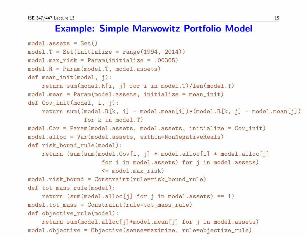
Example: Simple Marwowitz Portfolio Model

model.assets = Set()

model.T = Set(initialize = range(1994, 2014))

model.max_risk = Param(initialize = .00305)

model.R = Param(model.T, model.assets)

def mean_init(model, j):

return sum(model.R[i, j] for i in model.T)/len(model.T)

model.mean = Param(model.assets, initialize = mean_init)

def Cov_init(model, i, j):

return sum((model.R[k, i] - model.mean[i])*(model.R[k, j] - model.mean[j])

for k in model.T)

model.Cov = Param(model.assets, model.assets, initialize = Cov_init)

model.alloc = Var(model.assets, within=NonNegativeReals)

def risk_bound_rule(model):

return (sum(sum(model.Cov[i, j] * model.alloc[i] * model.alloc[j]

for i in model.assets) for j in model.assets)

<= model.max_risk)

model.risk_bound = Constraint(rule=risk_bound_rule)

def tot_mass_rule(model):

return (sum(model.alloc[j] for j in model.assets) == 1)

model.tot_mass = Constraint(rule=tot_mass_rule)

def objective_rule(model):

return sum(model.alloc[j]*model.mean[j] for j in model.assets)

model.objective = Objective(sense=maximize, rule=objective_rule)

15


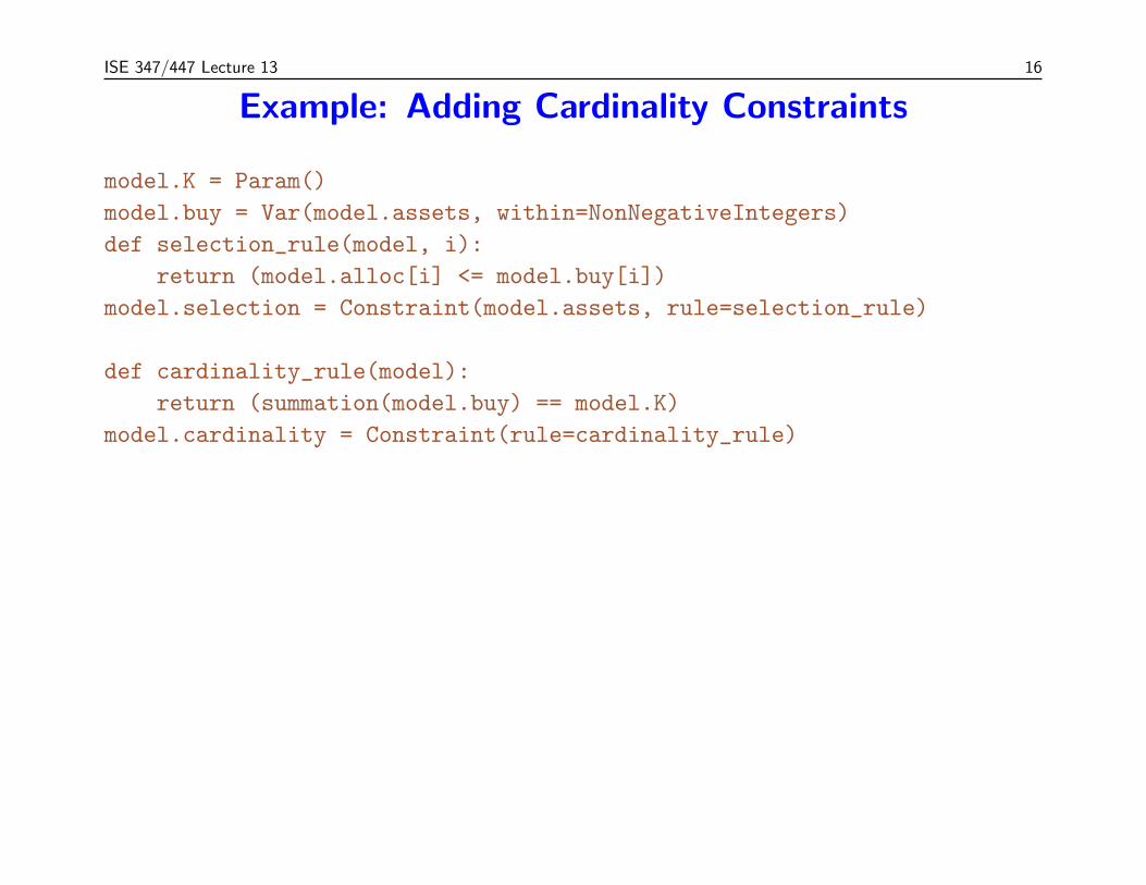
Example: Adding Cardinality Constraints

model.K = Param()

model.buy = Var(model.assets, within=NonNegativeIntegers)

def selection_rule(model, i):

return (model.alloc[i] <= model.buy[i])

model.selection = Constraint(model.assets, rule=selection_rule)

def cardinality_rule(model):

return (summation(model.buy) == model.K)

model.cardinality = Constraint(rule=cardinality_rule)

16


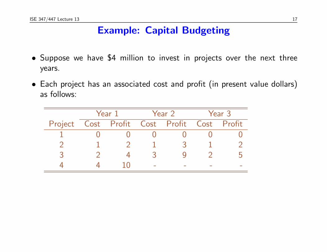
Example: Capital Budgeting

• Suppose we have $4 million to invest in projects over the next threeyears.

• Each project has an associated cost and profit (in present value dollars)as follows:

Year 1 Year 2 Year 3Project Cost Profit Cost Profit Cost Profit

1 0 0 0 0 0 02 1 2 1 3 1 23 2 4 3 9 2 54 4 10 - - - -

17


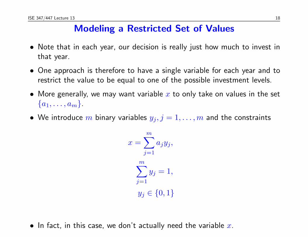
Modeling a Restricted Set of Values

• Note that in each year, our decision is really just how much to invest inthat year.

• One approach is therefore to have a single variable for each year and torestrict the value to be equal to one of the possible investment levels.

• More generally, we may want variable x to only take on values in the set{a1, . . . , am}.

• We introduce m binary variables yj, j = 1, . . . ,m and the constraints

x =

m∑j=1

ajyj,

m∑j=1

yj = 1,

yj ∈ {0, 1}

• In fact, in this case, we don’t actually need the variable x.

18


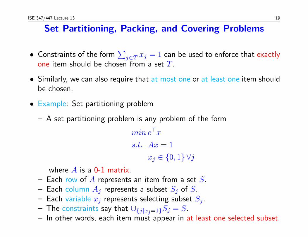
Set Partitioning, Packing, and Covering Problems

• Constraints of the form∑

j∈T xj = 1 can be used to enforce that exactlyone item should be chosen from a set T .

• Similarly, we can also require that at most one or at least one item shouldbe chosen.

• Example: Set partitioning problem

– A set partitioning problem is any problem of the form

min c>x

s.t. Ax = 1

xj ∈ {0, 1} ∀jwhere A is a 0-1 matrix.

– Each row of A represents an item from a set S.– Each column Aj represents a subset Sj of S.– Each variable xj represents selecting subset Sj.– The constraints say that ∪{j|xj=1}Sj = S.– In other words, each item must appear in at least one selected subset.

19


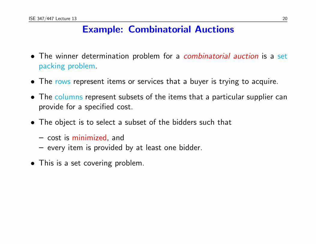
Example: Combinatorial Auctions

• The winner determination problem for a combinatorial auction is a setpacking problem.

• The rows represent items or services that a buyer is trying to acquire.

• The columns represent subsets of the items that a particular supplier canprovide for a specified cost.

• The object is to select a subset of the bidders such that

– cost is minimized, and– every item is provided by at least one bidder.

• This is a set covering problem.

20


Piecewise Linear Cost Functions

• We can use binary variables to model arbitrary piecewise linear costfunctions.

• We could use such a model to solve a version of the capital budgetingproblem in which we are allowed to invest in multiple projects, in wholeor in part.

• The function is specified by ordered pairs (ai, f(ai)) and we wish toevaluate it at a point x.

• We have a binary variable yi, which indicates whether ai ≤ x ≤ ai+1.

• To evaluate the function, we will take linear combinations∑k

i=1 λif(ai)of the given functions values.

• This works only if the only two nonzero λ′is are the ones correspondingto the endpoints of the interval in which x lies.

21


Minimizing Piecewise Linear Cost Functions

• The following formulation minimizes the function.

min

k∑i=1

λif(ai)

s.t.

k∑i=1

λi = 1,

λ1 ≤ y1,λi ≤ yi−1 + yi, i ∈ [2..k − 1],

λk ≤ yk−1,k−1∑i=1

yi = 1,

λi ≥ 0,

yi ∈ {0, 1}.

• The key is that if yj = 1, then λi = 0, ∀i 6= j, j + 1.

22


Fixed-charge Problems

• In many instances, there is a fixed cost and a variable cost associatedwith a particular decision.

• For example, there might be a fixed cost to certain financial transactions,regardless of the amount transacted.

• Consider the problem of converting B units of currency 1 into currency Nthrough a sequence of intermediate transactions in currencies 2 throughN − 1.

– To convert current i into a set of other currencies, there is a fixed costof ci (in terms of currency N).

– There is also an associated exchange rate rij.– There is a cap ui on the total amount of currency i that can be

converted.– The goal is to end up with as much of currency N as possible.

23


Modeling the Currency Exchange Problem

• The decision to be made is how much of each currency to exchange foreach other currency. So variables in this case areyi = whether any of currency i is exchanged for other currenciesxij = amount of currency i exchanged for currency j

• Note that the amount of currency j we end up with after exchangingfrom i is rijxij.

• Ultimately, we want to end up with as much of currency N as possible,so our objective function is the amount of all other currencies exchangedinto currency N :

max

N−1∑i=1

riNxiN −n∑

i=1

ciyi.

24


Modeling the Currency Exchange Problem (cont.)

• For notational convenience, we assume that xii = 0 ∀i ∈ [1..N ].

• For every currency j 6= 1, the amount available for exchange is∑N−1i=1 rijxij and the amount actually exchanged is

∑Nj=2 xij.

• The constraints are thenN∑j=2

xij ≤ yiui, ∀ i ∈ [1..N ],

N−1∑i=1

rijxij ≥N∑

k=2

xjk, ∀ j ∈ [2..N − 1],

N∑j=2

x1j ≤ B, and

xij ≥ 0, ∀ i ∈ [1..N − 1], j ∈ [2..N ].

yi ∈ {0, 1}, ∀ i ∈ [1..N − 1]

25


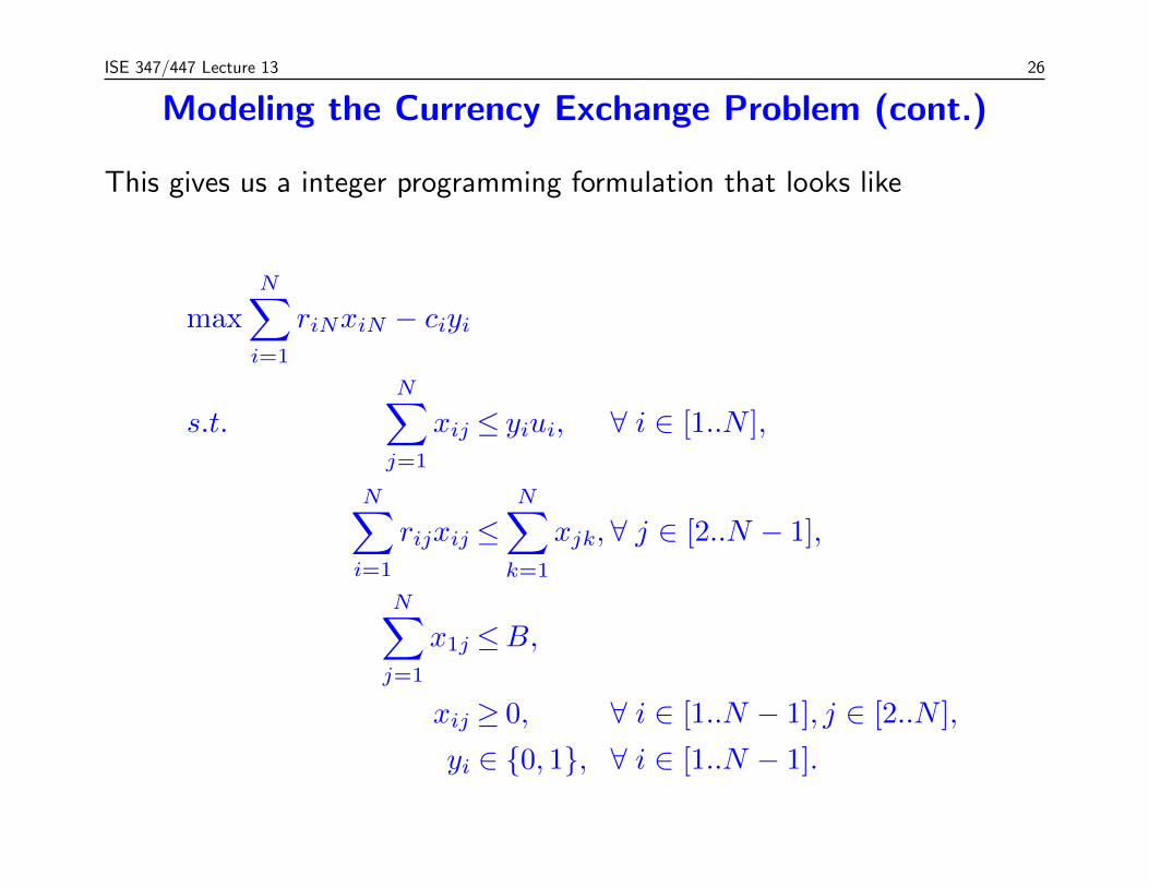
Modeling the Currency Exchange Problem (cont.)

This gives us a integer programming formulation that looks like

max

N∑i=1

riNxiN − ciyi

s.t.

N∑j=1

xij ≤ yiui, ∀ i ∈ [1..N ],

N∑i=1

rijxij ≤N∑

k=1

xjk, ∀ j ∈ [2..N − 1],

N∑j=1

x1j ≤B,

xij ≥ 0, ∀ i ∈ [1..N − 1], j ∈ [2..N ],

yi ∈ {0, 1}, ∀ i ∈ [1..N − 1].

26


Distinguishing “Formulations” and “Models”

• The modeling process consists generally of the following steps.

– Determine the “real-world” state variables, system constraints, andgoal(s) or objective(s) for operating the system.

– Translate these variables and constraints into the form of amathematical optimization problem (the “formulation”).

– Solve the mathematical optimization problem.– Interpret the solution in terms of the real-world system.

• This process presents many challenges.

– Simplifications may be required in order to ensure the eventualmathematical program is “tractable”.

– The mappings from the real-world system to the model and back aresometimes not very obvious.

– There may be more than one valid “formulation”.

• All in all, an intimate knowledge of mathematical optimization definitelyhelps during the modeling process.

27


The Importance of Fomulation

• Different formulations for the same problem can result in dramaticallydifferent in terms of tractability.

• Simple example: two ways of modeling binary variables x.

– x ∈ {0, 1}– x = x2

• The first formulation is integer linear, while the second formulation isnonlinear continuous.

• These would be solved with two entirely different classes of algorithms.

• As a rulse of thumb, the first formulation is preferred.

28

Financial Optimization ISE 347/447 Lecture 13ted/files/ie447/lectures/Lecture13.pdfISE 347/447...

Documents

Transcript of Financial Optimization ISE 347/447 Lecture 13ted/files/ie447/lectures/Lecture13.pdfISE 347/447...