Excel for Managers Lets get started T T he essentials managers need to know about Excel.
Upload
hung-pham-thaiCategory
view
702download
7description
with Excel® applications
Dawn E. Lorimer
Charles R. Rayhorn
second edition
ii
Library of Congress Cataloging-in-Publication Data
Lorimer, Dawn E., 1950- Financial modeling for managers : with Excel applications / Dawn E.Lorimer, Charles R. Rayhorn.— 2nd ed. p. cm.Rev. ed. of: Financial maths for managers / Dawn E. Lorimer, Charles R.Rayhorn. c1999.Includes bibliographical references and index. ISBN 0-9703333-1-5 (pbk.) 1. Business mathematics. 2. Microsoft Excel for Windows. 3.Electronic spreadsheets. 4. Financial futures. I. Rayhorn, Charles R.,1949- II. Lorimer, Dawn E., 1950- Financial maths for managers. III.Title. HF5691 .L58 2001 650'.01’513—dc21 2001005810
Copyright 2002 by Authors Academic Press
Financial Modeling for Managerswith Excel Applications
All rights reserved. Previous edition copyright 1999 by Dunmore Press Limited. Printed inthe United States of America. Except as permitted under the United States Copyright Act of1976, no part of this publication may be reproduced or distributed in any form or by anymeans, or stored in a data base or retrieval system, without the prior written permission ofthe publisher.
ISBN 0-9703333-1-5
Acquisition Editors: Trond Randoy, Jon Down, Don HerrmannSenior Production Manager: Cynthia LeonardLayout Support: Rebecca HerschellMarketing Manager: Nada DownCopyeditor: Michelle AbbottCover Design: Tom Fenske and Cynthia LeonardCover Photo: London Dealing Room. Courtesy National Australia Bank, London.Printer: EP Imaging Concepts
AcknowledgmentsRobert Miller—Northern Michigan University, Michael G. Erickson—Albertson College, andJacquelynne McLellan—Frostburg State University all contributed greatly to the production ofthis book through their thoughtful reviews.
When ordering this title, use ISBN 0-9703333-1-5
www.AuthorsAP.com

iii
ContentsContents
Preface ........................................................................................................1
Part I. Interest rates and foreign exchange
Chapter 1: Compounding and discounting 7
Chapter 2: The valuation of cash flows 31
Chapter 3: Zero’s, forwards, and the term structure 73
CONTENTS
1.1 Notation and definitions ......................................................................... 81.2 Time value of money ............................................................................. 81.3 Simple interest, bills and other money market securities ...................... 101.4 Compound interest ................................................................................ 161.5 Linear interpolation ............................................................................... 191.6 Real interest rates ................................................................................. 20
2.1 Notation and definitions ........................................................................ 322.2 Cash flow representation ...................................................................... 342.3 Valuing annuities ................................................................................... 362.4 Quotation of interest rates .................................................................... 392.5 Continuous time compounding and discounting ..................................... 442.6 Fixed interest securities ........................................................................ 472.7 Duration and value sensitivity ............................................................... 572.8 Interest rate futures .............................................................................. 61
3.1 Notation and definitions ........................................................................ 743.2 A brief mystery of time ....................................................................... 753.3 Zero coupon rates ................................................................................. 763.4 Implied forward rates ........................................................................... 793.5 Forwards, futures and no-arbitrage ...................................................... 813.6 Computing zeros and forwards ............................................................. 863.7 Algorithm: computing zeros and forwards from swap data ................. 893.8 Concluding remarks .............................................................................. 97

iv
Chapter 4: FX Spot and forwards 103
Part II. Doing it the Excel® way
Chapter 5: Learning by doing: an introduction to financial spreadsheets 127
Part III. Statistical analysis and probability processes
Chapter 6: Statistics without becoming one 151
Chapter 7: Regression and financial modeling 175
4.1 Notation and definitions ...................................................................... 1044.2 Spot exchange rate quotations ............................................................ 1054.3 Inversions ............................................................................................ 1084.4 Cross rates .......................................................................................... 1094.5 Money market forward rates .............................................................. 114
5.1 Step-by-step bond valuation example ................................................. 1285.2 Do-it-yourself fixed interest workshop ............................................... 137
6.1 Notation and definitions ...................................................................... 1526.2 Introduction to data ............................................................................. 1536.3 Downloading data .............................................................................. 1546.4 Data exploration ................................................................................. 1566.5 Summary measures ............................................................................ 1596.6 Distribution function and densities ...................................................... 1646.7 Sampling distributions and hypothesis testing ...................................... 168
7.1 Notation and definitions ...................................................................... 1767.2 Bivariate data exploration ................................................................... 1777.3 Regression statistics .......................................................................... 1827.4 More regression theory: goodness of fit ............................................ 1877.5 The CAPM beta ................................................................................. 1897.6 Regression extensions: multiple regression ........................................ 196

v
Chapter 8: Introduction to stochastic processes 203
Part IV. Many variables
Chapter 9: Many variables 235
Part V. Appendix
General Mathematical review 264
8.1 Notation and definitions ...................................................................... 2048.2 Expectations ....................................................................................... 2058.3 Hedging ............................................................................................... 2068.4 Random walks and Ito processes. ...................................................... 2138.5 How Ito processes are used ............................................................... 2178.6 Volatility models .................................................................................. 2238.7 Other time series buzzwords .............................................................. 226
9.1 Vectors and matrices .......................................................................... 2369.2 Matrix inverses and equation solving .................................................. 2409.3 Statistics with matrices ....................................................................... 2439.4 Portfolio theory with matrices ........................................................... 2459.5 Practicum ............................................................................................ 248
A1 Order of operations ............................................................................. 264A2 Multiplication and division with signed numbers ................................. 265A3 Powers and indices ............................................................................. 267A4 Logarithms .......................................................................................... 272A5 Calculus .............................................................................................. 273

vi

1
We wrote the book because we felt that financial professionals needed it; andthose who are training to be financial professionals, as students in colleges, willneed it by the time they finish. Not all of us are cut out to be Quants, or would evenwant to. But pretty much all of us in the financial world will sooner or later have tocome to grips with two things. The first is basic financial math and models. Thesecond is spreadsheeting. So we thought that the market should have a book thatcombined both.
The origins of the book lie in financial market experience, where one of us (DEL),at the time running a swaps desk, had the problem of training staff fresh fromcolleges, even good universities, who arrived in a non operational state. Rather likea kitset that had to be assembled on the job: you know the bits are all there, but theycan’t begin to work until someone puts all the bits together. Their theoreticalknowledge might or might not have been OK, but instead of hitting the groundrunning, the new graduates collapsed in a heap when faced with the “what do I dohere and now?” problem. The present book evolved out of notes and instructionalguidelines developed at the time. In later versions, the notes took on an internationalflavor and in doing so, acquired a co author (CH), to become the present book,suitable for the U.S. and other international markets.
The material you will find here has been selected for maximal relevance for theday to day jobs that you will find in the financial world, especially those concernedwith financial markets, or running a corporate treasury. Everything that is here, sofar as topics are concerned, you can dig up from some theoretical book or journalarticle in finance or financial economics. But the first problem is that busy
PrefaceWHY READ THIS BOOK?

2
professionals simply do not have the time to go on library hunts. The second problemis that even if you do manage to find them, the techniques and topics are notimplemented in terms of the kind of computational methods in almost universal usethese days, namely Excel or similar spreadsheets.
No spreadsheet, no solution, and that is pretty well how things stand throughout thefinancial world. Students who graduate without solid spreadsheeting skillsautomatically start out behind the eight ball. Of course, depending on where youwork, there can be special purpose packages; treasury systems, funds managementsystems, database systems, and the like, and some of them are very good. But it isinadvisable to become completely locked into special purpose packages, for a numberof reasons. For one thing, they are too specialized, and for another, they are subjectto “package capture”, where firms become expensively locked into serviceagreements or upgrades. So in our own courses, whether at colleges or in themarkets, we stress the flexibility and relative independence offered by a multipurposepackage such as Excel or Lotus. Most practitioners continue to hedge their specialsystems around with Excel spreadsheets. Others who might use econometric orsimilar data crunching packages, continue to use Excel for operations like basicdata handling or graphing. So, spreadsheets are the universal data and money handlingtool.It is also a truism that the financial world is going high tech in its methodologies,which can become bewildering to managers faced with the latest buzzwords, usuallyacronymic and often incomprehensible. This leaves the manager at a moraldisadvantage, and can become quite expensive in terms of “consultant capture”. Inwriting the book we also wanted to address this credibility gap, by showing thatsome, at least, of the buzzwords can be understood in relatively plain terms, andcan even be spreadsheeted in one or two cases. So without trying to belittle thequants, or the consultants who trade in their work, we are striking a blow here forthe common manager.
It remains to thank the many people who have helped us in preparing the book. Asthe project progressed, more and more people from the financial and academiccommunities became involved, and some must be singled out for special mention.Larry Grannan from the Chicago Mercantile Exchange responded quickly to ourquestions on CME futures contracts. Cayne Dunnett from the National Bank ofAustralia (NAB) in London gave generously of his time to advise us on financialcalculations. Together with Ken Pipe, he also organized the photo shoot for thefront cover, taken in the NAB’s new London dealing room. Joe D’Maio from theNew York office of the NAB pitched in with assistance on market conventions andproducts. Andy Morris at Westpac in New York provided helpful information onUS financial products. Penny Ford from the BNZ in Wellington, New Zealandkindly assisted with technical advice and data.

3
Among the academic community, Jacquelynne McLellan from Frostburg StateUniversity in Maryland and Michael G. Erickson from Albertson College in Ohioread the entire manuscript and took the trouble to make detailed comments andrecommendations. Roger Bowden at Victoria University of Wellington read throughthe manuscript making many helpful suggestions, and kept us straight on stochasticprocesses and econometric buzzwords. Finally, it has been great working withCynthia Leonard and Tom Fenske of Authors Academic Press. They have beenencouraging, patient, and responsive at all times, which has made this project apositive experience for all.

4

Part OneINTEREST RATES AND FOREIGN EXCHANGE
5
In the world of finance, interest rates affect everyone and everything. Of course,this will be perfectly obvious to you if you work in a bank, a corporate treasury, orif you have a home mortgage. But even if you work in equities management – orare yourself an investor in such – you will need to have some sort of familiaritywith the world of fixed interest: the terms, the conventions and the pricing. Wheninterest rates go up, stock prices go down; and bonds are always an alternative toequities, or part of a portfolio that might include both.
So the conventions and computations of interest rates and the pricing of instrumentsthat depend on interest rates are basic facts of life. We have another agenda inputting the discussion of interest rates first. Many readers from the industry willneed to get back into the swing of things so far as playing around with symbols andnumbers is concerned, and even students might like a refresher. Fixed interestarithmetic is a excellent way to do this, for the math is not all that complicated initself, and the manipulation skills that you need are easily developed without havingto puzzle over each step, or feel intimidated that the concepts are so high-poweredthat it will need ten tons of ginseng to get through it all. Once you have built up a bitof confidence with the basic skills, then you can think about going long in ginsengfor the chapters that follow.
As well as interest rates, we have inserted a chapter on the arithmetic of foreignexchange, incorporating the quotation, pricing and trading of foreign currencies formuch the same reasons. These days everyone has to know a bit about the subject,and again, the math is not all that demanding, although in a practical situation youreally do have to keep your wits about you.
You will notice that Excel is not explicitly introduced in Part 1. We do this in Part2, where we can use the material of Part 1 to generate some computable examples.In the meantime, it is important that you can execute the interest rate arithmetic ona hand-calculator. Practically any commercial calculator (apart from the simpleaccounting ones) will have all the functions that you need, and indeed most can beexecuted using a very basic classroom scientific type calculator – it just takes a bitlonger. The beauty of acquiring a true financial calculator is that in addition tospecial functions like the internal rate of return, it has several storage locations,useful for holding intermediate results when solving more complex problems. Atany rate, keep a calculator nearby as you read on.

6

OneOneOneOneOneCompounding and Discounting
7
This chapter has two objectives. The first is to review some basic interest rateconventions. Here we address questions like, what is the true rate of interest on adeal? Is it what you see in the ad, what the dealer quoted you over the phone, orsomething different altogether? And how does this rate compare with what isoffered elsewhere?
The interest rate jungle is in some respects like shopping for a used car - you can getsome good deals, but also some pretty disastrous ones, where the true cost is hiddenbeneath a fancy PR package. Unless you know what you are doing, things can getpretty expensive.
The second objective is to introduce you to the market ambience where interestrates are quoted. In this chapter, we are largely concerned with money marketinstruments, which are a particular sort of fixed interest instrument used by corporatetreasurers every day. Even if you are not a corporate treasurer, you are surely yourown personal treasurer, and knowing about these instruments will help you in yourown financing and investment decisions. Studying these instruments will sharpenyour understanding of the interest rate concept.

Part I. Interest Rates and Foreign Exchange
8
Financial Modeling for Managers
1.1 Notation and definitions
APR Annual percentage interest.
FV Future value of money, which is the dollar amount expected to be receivedin the future. It generally includes amounts of principal and interest earnings.
PV Present value of money, the value today of cash flows expected in thefuture discounted at an (or in some situations at more than one) appropriaterate.
Pt
The price at time t. Can also stand for the principal outstanding at time t.
i Symbol for the effective interest rate, generally expressed as a decimal.Can vary over time, in which case often indexed as i
t.
I Total money amount of interest earned.
D Number of days to maturity.
Dpy Number of days per year. Determined by convention, usually 365 or 360days.
n Number of years (greater than one). Can be fractional.
m Number of compounding periods in a year
C The amount of the periodic payment or coupon.
π The rate of inflation.
1.2 Time value of money
There's a saying that time is money. An amount of money due today is worth morethan the same amount due some time in the future. This is because the amount dueearlier can be invested and increased with earnings by the later date. Many financialagreements are based on a flow (or flows) of money happening in the future (forinstance, housing mortgages, government bonds, hire purchase agreements). Tomake informed financial decisions, it is crucial to understand the role that time playsin valuing flows of money.
9
Chapter One. Compounding and Discounting
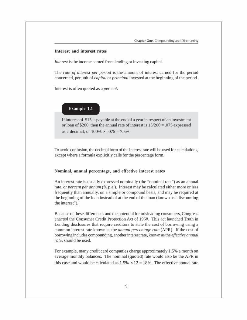
Interest and interest rates
Interest is the income earned from lending or investing capital.
The rate of interest per period is the amount of interest earned for the periodconcerned, per unit of capital or principal invested at the beginning of the period.
Interest is often quoted as a percent.
If interest of $15 is payable at the end of a year in respect of an investmentor loan of $200, then the annual rate of interest is 15/200 = .075 expressed
as a decimal, or 100% × .075 = 7.5%.
Example 1.1
To avoid confusion, the decimal form of the interest rate will be used for calculations,except where a formula explicitly calls for the percentage form.
Nominal, annual percentage, and effective interest rates
An interest rate is usually expressed nominally (the “nominal rate”) as an annualrate, or percent per annum (% p.a.). Interest may be calculated either more or lessfrequently than annually, on a simple or compound basis, and may be required atthe beginning of the loan instead of at the end of the loan (known as “discountingthe interest”).
Because of these differences and the potential for misleading consumers, Congressenacted the Consumer Credit Protection Act of 1968. This act launched Truth inLending disclosures that require creditors to state the cost of borrowing using acommon interest rate known as the annual percentage rate (APR). If the cost ofborrowing includes compounding, another interest rate, known as the effective annualrate, should be used.
For example, many credit card companies charge approximately 1.5% a month onaverage monthly balances. The nominal (quoted) rate would also be the APR in
this case and would be calculated as 1.5% × 12 = 18%. The effective annual rate

Part I. Interest Rates and Foreign Exchange
10
Financial Modeling for Managers
would actually be higher because of compounding, a subject we will discuss inmore detail later. The effective rate would be calculated as ((1 + .015)12 - 1) ×100% or 19.6%. In general, the effective rate can be calculated by replacing 12 bythe number of compounding periods (m) during the year. Thus, the equation for theeffective rate is:
((1 + i)m - 1) × 100% (1)
Let's look at a situation where the nominal rate and the APR are not the same.The nominal and APR are always different when interest has to be prepaid orwhen there are fees associated with getting a particular nominal interest rate (e.g.points). Many loans on accounts receivable require the interest on the loan to bededucted from the loan proceeds. This is known as prepaying the interest. Forexample, let's assume that the nominal rate is 6.00% for one year and that theinterest has to be 'prepaid'. If the loan is for $1000.00, the loan proceeds in thiscase would be $940.00, or $1000.00 - .06 × ($1000.00). The APR in this exampleis $60.00/$940.00 or about 6.38%. Without truth in lending, the lending institutioncould claim that the cost of the loan is actually lower than it is. The effective ratewould also be 6.38% because there is only one compounding period.
There will be more on nominal and effective rates later. These are importantconcepts for anyone involved with financial transactions.
1.3 Simple interest, bills and other money market securities
The use of simple interest in financial markets is confined mainly to short termtransactions (less than a year), where the absence of compounding is of littleimportance and where the practice of performing calculations quickly, before moderncomputing aids became widely available, was necessary.
Simple interest can be misleading if used for valuation of long term transactions.Hence, its application in financial markets is usually limited to the calculation ofinterest on short-term debt and the pricing of money market securities.
When the interest for any period is charged only on the original principal outstanding,it is called simple interest. (In this situation, no interest is earned on interestaccumulated in a previous period.) That is:

11
Chapter One. Compounding and Discounting
Simple interest amount = Original Principal × Interest Rate × Term of interestperiod
In symbols: I = P0 × i × t (2)
where t = Ddpy
Here there is no calculation of interest on interest; hence, the interest amount earnedper period is constant.
Future value
In a simple interest environment:
FV = P0 + I = P
0 + (P
0 × i × t)
That is, FV = P0 (1 + (i × t)) (3)
where t = Ddpy
Calculate the amount of interest earned on a deposit of $1m for 45 days atan annual interest rate p.a. of 4.75%. What is the future value of thisdeposit?
Interest = P0 × i × t = $1,000,000 × .0475 × = $5,856.16
FV = P0 + I = P
0 (1 + (i × t)) = $1,000,000 (1 + (.0475 × ))
= $1,005,856.16
Example 1.2
45365
45365

Part I. Interest Rates and Foreign Exchange
12
Financial Modeling for Managers
Present value
Formula (3) may be rearranged by dividing by (1 + (i × t)) so that:
PV = P0 = ))(1( ti
FV
×+ (4)
In this case, the original principal, P0, is the present value and therefore the price
to be paid for the FV due after t years (where t is generally a fraction) calculatedat a yield of i.
There are two methods used for pricing money market securities in the US: thebank discount and the bond equivalent yield approach. Examples of moneymarket securities that are priced using the discount method include U.S. TreasuryBills, Commercial Paper, and Bankers’ acceptances. Formula (4) can’t be useddirectly for valuing these securities because of the particular rate, the bank discountrate, which is usually quoted (see below).
Examples of money market securities that are discounted using the bond equivalentyield approach include Certificates of Deposit (CD’s), repos and reverses, andFederal Funds. Also, short dated coupon-paying securities with only one morecoupon (interest payment) from the issuer due to the purchaser, and floating ratenotes with interest paid in arrears can fit into this category. For money marketinstruments using the bond equivalent yield, Formula (4) can be used directly.
There are two key differences involved in these pricing methods. The bondequivalent yield uses a true present value calculation and a 365-day year. It appliesan interest rate appropriately represented as the interest amount divided by thestarting principal. The bank discount method uses a 360-day year and it does notuse a normal present value calculation. The interest rate in this case is taken as the
Calculate the PV of $1m payable in 192 days at 4.95% p.a. on 365-dpybasis.
PV = = = $974,622.43
Example 1.3
FV(1 + (i × t))
$1,000,000(1 + (.0495 × 192 ÷ 365))
13
Chapter One. Compounding and Discounting
difference between the FV and the price of the instrument divided by the FV.Examples and solutions are provided in the following sections.
The appendix to this chapter describes the most frequently used money marketinstruments.
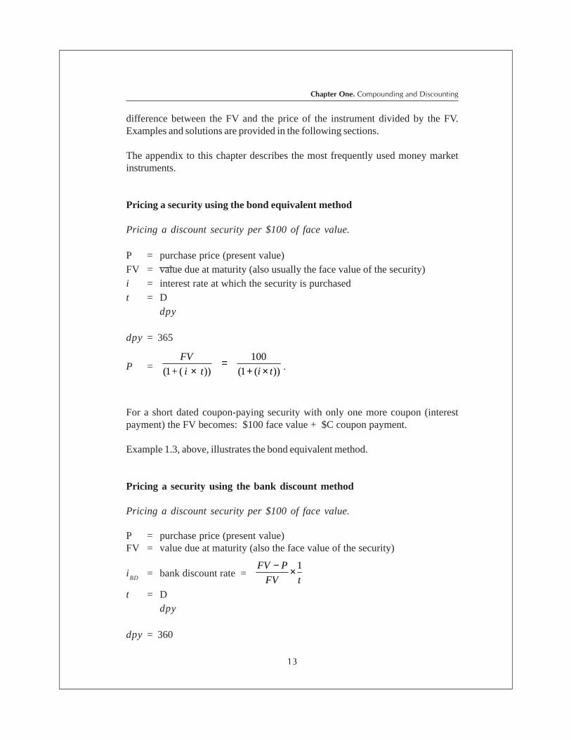
Pricing a security using the bond equivalent method
Pricing a discount security per $100 of face value.
P = purchase price (present value)FV = value due at maturity (also usually the face value of the security)i = interest rate at which the security is purchasedt = D
dpy
dpy = 365
P = ti
t i +
FV
))(1(
100
))(1( ×+=
× .
For a short dated coupon-paying security with only one more coupon (interestpayment) the FV becomes: $100 face value + $C coupon payment.
Example 1.3, above, illustrates the bond equivalent method.
Pricing a security using the bank discount method
Pricing a discount security per $100 of face value.
P = purchase price (present value)FV = value due at maturity (also the face value of the security)
iBD
= bank discount rate = tFV
PFV 1×−
t = Ddpy
dpy = 360
Part I. Interest Rates and Foreign Exchange
14
Financial Modeling for Managers
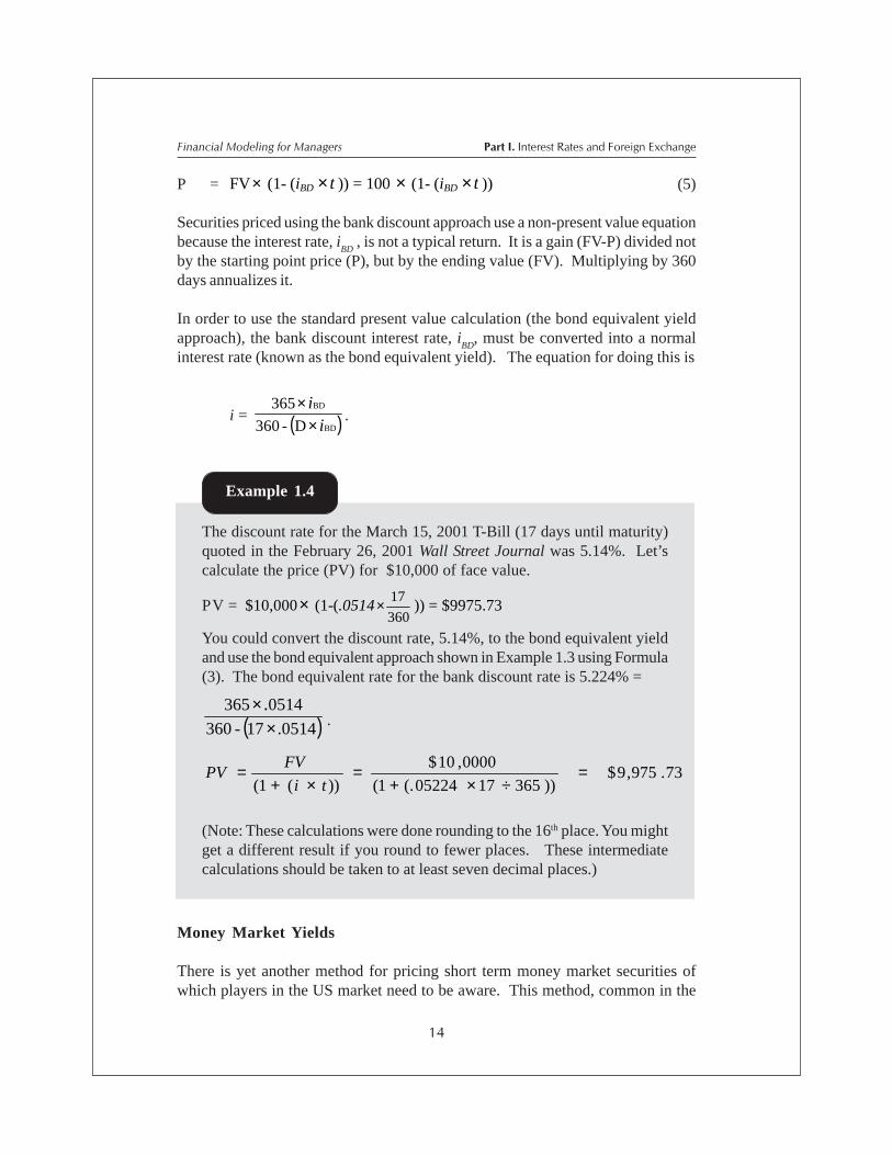
The discount rate for the March 15, 2001 T-Bill (17 days until maturity)quoted in the February 26, 2001 Wall Street Journal was 5.14%. Let’scalculate the price (PV) for $10,000 of face value.
PV = $10,000× (1-(.0514360
17× )) = $9975.73
You could convert the discount rate, 5.14%, to the bond equivalent yieldand use the bond equivalent approach shown in Example 1.3 using Formula(3). The bond equivalent rate for the bank discount rate is 5.224% =
( ).051417-360
0514365 . ×
×.
73.975,9$))3651705224(.1(
0000,10$
))(1(=
÷×+=
×+=
ti
FVPV
(Note: These calculations were done rounding to the 16th place. You mightget a different result if you round to fewer places. These intermediatecalculations should be taken to at least seven decimal places.)
Example 1.4
P = FV× (1- (iBD t× )) = 100 × (1- (iBD t× )) (5)
Securities priced using the bank discount approach use a non-present value equationbecause the interest rate, i
BD , is not a typical return. It is a gain (FV-P) divided not
by the starting point price (P), but by the ending value (FV). Multiplying by 360days annualizes it.
In order to use the standard present value calculation (the bond equivalent yieldapproach), the bank discount interest rate, i
BD, must be converted into a normal
interest rate (known as the bond equivalent yield). The equation for doing this is
i = ( )BD
BD
D-360
365 i
i×
×.
Money Market Yields
There is yet another method for pricing short term money market securities ofwhich players in the US market need to be aware. This method, common in the

15
Chapter One. Compounding and Discounting
Eurodollar markets, uses money market yields with interest calculated as:
Interest = Face Value × [iMMY × d / 360)]
The price of such an instrument is calculated using the same technique as the bondequivalent method, but the days per year (dpy) is taken to be 360 days.
A note on market yield
Short-term securities are quoted at a rate of interest assuming that the instrumentis held to maturity. If the instrument is sold prior to maturity, it will probablyachieve a return that is higher or lower than the yield to maturity as a result ofcapital gains or losses at the time it is sold. In such cases, a more useful measureof return is the holding period yield.
Holding period yield (for short-term securities)
The holding period yield (Yhp
) is the yield earned on an investment between thetime it is purchased and the time it is sold, where that investment is sold prior tomaturity. For short-term securities, this is calculated as:
Yhp = t
1 - P/ P buysell , (6)
where t is defined above (a fraction of a year), Psell
is the price at which you soldthe security, and P
buy is the price at which you bought it.
Suppose the investor from Example 1.4 sold the T-bill (previously purchasedat a bank discount rate of 5.14%) at a new discount rate of 5.10% whenthe bill had just three days to run to maturity. The selling price is calculated:
PV= $10,000× (1- (.0510360
3× )) = $9995.75
The holding period yield p.a. is:
. = =
= Y hp %23.50.0523)365/14(
1)9975.73/75.995,9( −
Example 1.5

Part I. Interest Rates and Foreign Exchange
16
Financial Modeling for Managers
1.4 Compound interest
Compound interest rates mean that interest is earned on interest previously paid.Bonds are priced on this basis and most bank loans are as well. Many depositaccounts also have interest calculated on a compound basis. Before we formalizethings, let’s start with a few examples.
In general, the formula for accumulating an amount of money for n periods ateffective rate i per period (or for calculating its future value) is:
AV = FV = P0 × (1 + i) n (7)
or FV = PV × (1 + i)n (again, AV = FV)
Note that this formula refers to n periods at effective rate i per period. Thus, n andi can relate to quarterly, monthly, semi annual, or annual periods.
It is easy to see that Formula (7) can be rearranged to give a formula for thepresent value at time 0 of a payment of FV at time n.
PV = P0 = ni
FV
)1( + = FV × (1+i)-n (8)
$100 invested at 5% annual interest would be worth $105 in one year’stime.
If the same investment is held for two years at 5% and the interestcompounds annually, the future value of the investment is:
FV = $105 × (1 + .05) = $110.25 That is, FV = $100 × (1.05) × (1.05) = $100 × (1.05) 2
At the end of three years, assuming the same compound interest rate, theinvestment would have an accumulated value of:
$100 × (1.05) 3 = $115.76
Example 1.6

17
Chapter One. Compounding and Discounting
Find accumulated value of $1000 after 5 1/4 years at 6.2% per annumcompound interest.
Solution 1.7
P0
= 1000, n = 5.25, i = 0/062
AV = P0(1 + i )n
AV = 1000(1.062)5.25
= 1000(1.371367)= $1,371.37
Example 1.7
Find the present value of $1,000,000 due in three years and 127 days fromtoday where interest compounds each year at 6.25% p.a. Assume a 365-day year, so that 127 days is equal to 0.3479452 of a year.
Solution 1.8
PV = $1,000,000 (1.0625)-3.3479452
= $816,304.43
Example 1.8
In some cases we may wish to value cash flows to a specific date that is neitherthe end date of the final cash flow nor the current date. The following exampleillustrates the technique for calculating an accumulated value or future value to aspecific date prior to the final cash flow.
The following problems illustrate how to find the future or accumulated value andthe present value of single cash flows.

Part I. Interest Rates and Foreign Exchange
18
Financial Modeling for Managers
Find the value at one year and 60 days from today of $1 million due in twoyears and 132 days from today, where interest compounds at 6.5% p.a.Assume a 365-day year.
Solution 1.9
Preliminary calculations:132 / 365 = 0.3616438460 / 365 = 0.16438356
PV = P0
= FV(1 + i)-n = $1,000,000 (1.065)-2.36164384
Value at time t = P0(1 + i)t
= $1,000,000(1.065)-2.36164384(1.065)1.16438356
= $1,000,000(1.065)-(2.36164384-1.16438356)
Hence, the value at time t = Vt = P
0(1 + i)t = AV( 1 + i )-n ( 1 + i )t
= AV(1 + i )-(n-t)
Example 1.9
Multiple interest rates
For money market funds, NOW accounts, sweep accounts (a variation on moneymarket funds and NOW accounts), and other investments, interest is payable onthe previous balance (interest and principal) at the prevailing market interest rate.Since the interest rate may change from period to period, multiple rates of interestmight apply, but we’ll stick with basic concepts for now.
Find the future (i.e. accumulated) value of $10,000 invested at 6% compoundfor two years, and 7% p.a. compound interest for the following four years.
FV = $10,000(1.06) 2(1.07) 4 = $14,728.10
Example 1.10

19
Chapter One. Compounding and Discounting
1.5 Linear interpolation
In many financial situations, it is necessary to estimate a particular value that fallsbetween two other known values. The method often used for estimation is calledlinear interpolation. (There are other forms of interpolation; however, they arebeyond the scope of this book.)
Suppose that you know the interest rates at two maturity points on a yieldcurve and are trying to estimate a rate that falls at some maturity betweenthese two points.
Figure 1.1 Linear interpolation
The yield curve here is clearly not a simple linear function, but a linearapproximation between two relatively close points will not be too far offthe curve.
We know that the one-year rate is 4.2% and the two-year rate is 5.3%.The linear interpolation for 1.5 years will be 4.75%, or 4.2 + 5.3)/2 . Wherethe desired interpolation is not the mid-point between the two known points,the following weighting can be applied.
Using the above two points, suppose that we wish to find an interpolatedrate for one year and 40 days (or 1.109589 years). A picture often clarifiesour thinking, so let i
1.109589, the rate we are seeking, be equal to ∆%, and
draw a timeline for it = f (time).
Example 1.11
� �
����������
������ ��������

Part I. Interest Rates and Foreign Exchange
20
Financial Modeling for Managers
1.0 1.109589 2.0
_____________________________ A B C
it = f (time) 4.2% 5.3%
Figure 1.2 Timeline
Length AB = 1.109589 - 1.0 = .109589
Length BC = 2.0 - 1.109589 = .890411
Length AC = 2.0 - 1.0 = 1.0
The ratio AB = .109589 = .109589AC 1.0
and BC = .890411 = .890411AC 1.0
The above problem is like the reverse of a seesaw. When you have playersof different weights the heavier one must sit closer to the balancing point ofthe seesaw. Here we have shifted the fulcrum of the seesaw and mustplace the heavier weight on the shorter end to achieve a balance. Theabove ratios are treated as the weights that we apply to find ∆ as follows:
∆ = {(4.2% × .890411) + (5.3% × .109589)} = 4.3205479%
The interpolated rate i for one year and 40 days that we have called ∆ istherefore equal to 4.3205% (rounded to four decimals).
The above interpolation method is used for a number of financial problems.
It can be applied, for example, to the selection of hedge ratios where morethan one instrument is used to hedge the underlying exposure.
1.6 Real interest rates
In Section 1.2 of this chapter, we introduced the concept of interest and interestrates without giving their economic purpose. Everybody knows that a dollar todayis not the same as a dollar tomorrow because we can invest this dollar to earn
∆∆∆∆∆

21
Chapter One. Compounding and Discounting
interest. But why is interest offered? There are many reasons and entire bookshave been written on the subject. We will briefly describe three.
First, it is assumed that people would rather consume their incomes now ratherthan in the future. To induce people to save part of their income and forgo currentconsumption, a monetary inducement must be paid. The more you enjoy currentconsumption, the more you must be paid to save. The incentive that you are paid tosave is the dollar amount of interest, which as we already know can be expressedas an interest rate. This preference for current consumption is known as your timepreference for consumption. The higher the time preference, the higher the interestrate needed to encourage savings.
The second dimension to this story is risk, which comes in various flavors. Oneaspect is the likelihood that your savings will be paid back (along with the interest).The more uncertain you are that you will be paid back (the probability of loss, orrisk), the higher the monetary inducement you will demand in order to save. It isbeyond the scope of this book to talk about the many aspects of risk, but theunderlying principle is that the higher the risk, the higher the interest (or monetaryinducement) demanded.
The final dimension of why interest rates exist is inflation. Inflation is the increasein the level of consumer prices, or a persistent decline in the purchasing power ofmoney. Suppose that you had a zero time preference for consumption, so youdidn’t demand interest for saving. Further suppose that you knew with certaintythat the future cash flow would materialize, meaning again, you don’t require interestto save. In such a scenario, you would still have to charge interest equal to the rateof inflation, just to stay even.
Taken together, these three dimensions make up what is known as the nominalrate of interest. When we remove one of these dimensions—the last one, inflation—we are talking about the real rate of interest. The real rate of interest is theexcess interest rate over the inflation rate, which can be thought of as the purchasingpower derived from an investment.
Suppose the rate of inflation is 10%. How much in today’s (time 0) purchasingpower is $1 worth when received in the future (time 1)? The answer is 1/1.1 =$0.91 (notice that this is Equation (9), where n = 1). Now suppose that you earned10% interest over the unit time period. Your real command over goods and servicesat the end of the period would be 1.1 times 0.91, or $1 worth of purchasing power—exactly the same as what you started with. The only way this can happen is if thereal rate of interest you have earned is zero percent. What you gained on thenominal rate of interest of 10%, you lost on the devalued dollar at the end of theperiod. In this case, the purchasing power derived from this investment is zero.
Part I. Interest Rates and Foreign Exchange
22
Financial Modeling for Managers
Let us generalize this a bit. Let π be the rate of inflation, and let i be the nominalrate of interest. Then the real rate i
* is defined as:
1+ i*
= )1(
)1(
+
i
π+
i*
=)1(
)1(
+
i
π+
-1 (9)
In other words, the real compounding factor (1+i*) is equal to the nominal
compounding factor discounted by the rate of inflation.
This is the technical definition, and the one that ought to be used when you operatein discrete time, as we did here. You sometimes see an alternative definition of thereal rate as simply the nominal rate less the rate of inflation. With a bit of rearranging,Equation (9) can be written:
i*
= .])1(
1)[( ππ
ππ - i +
- i ≈− (10)
The sign ≈ means, “approximately equal to.” We are saying that the real rate isapproximately equal to the difference between the nominal rate i, and the rate ofinflation p. You can see that the approximation works only if the rate of inflation islow; otherwise, the second term in the square brackets is not small. This alternativedefinition is convenient because it can be calculated in your head and gives you aquick idea of the real rate of interest. However, it is only an approximation.
The rate of inflation is just the percentage change of some suitable price index.Choosing which version of the price index to use—the consumer price index or theGDP deflator—is a point of debate. In this case, we are talking about changes inreal wealth and need some sense of what that wealth can buy in terms of consumergoods and services, so the consumer price index is probably the better choice.However, the GDP deflator or some other measure of inflation may be moreappropriate in a different decision problem.
This may not mean much to you if you are not an economist. It’s probably true thatit’s the economists who are most interested in the real rate of interest. However,sometimes capital budgeting problems, personal financial planning problems, andthe like, are cast in terms of real future cash flows, meaning that they are adjustedfor the reduced purchasing power of money at those future dates. In such cases,the real rate of interest must be used in discounting. The general rule is: Likediscounts like. If your cash flows are nominal, use nominal rates; if your cashflows are real, use real rates.

23
Chapter One. Compounding and Discounting
A similar principle applies where the cash flows are measured on an after-taxbasis. In this case, you have to use an after-tax rate of interest, which is usuallycalculated by multiplying the nominal rate by (1 - t), where t is the applicable rateof tax. Again, this is an approximation, valid if the product i × t is negligible in size.You might have fun trying to define a “real after-tax rate of interest,” but don’t askus!
At any rate, the nominal rate of interest will be used throughout this book and isused in almost all market dealings.
Money Market Instruments
24
App
endi
x 1
U.S. Treasury Bills (T-Bills)
T-Bills are direct obligations of the United States federal government. They areissued at a discount for periods of three months (91 days), six months (182 days),or one year (52 weeks). Since Treasury bills are the most marketable of all moneymarket securities they have been, and continue to be, a popular investment forshort-term cash surpluses. T-Bills can be purchased at inception via a direct auctionor in an active secondary market that provides instant liquidity. The income earnedon T-Bills is taxed at the federal level only. They are sold at a discount and theprice is calculated using the bank discount method.
Certificates of Deposit (CD)
A certificate of deposit is a time deposit with a bank, with interest and principal paidto the depositor at the end of the fixed term of the CD. The denominations of CDsare at will, ranging from $500 to over $100,000. As with other deposits in banks,the Federal Deposit Insurance Corporation insures CD’s up to the first $100,000.For smaller (retail) CDs of $100,000 or less, banks can impose interest penaltieswhere depositors wish to withdraw funds prior to maturity of the contract. Large(wholesale) CDs, over $100,000, cannot be withdrawn on demand but are readilymarketable, while smaller CDs are not. The secondary market for these largerCD’s thins as the maturity lengthens. The price of marketable CD’s is the presentvalue of the principal and interest at maturity using the bond equivalent yield approach.
Bankers’ Acceptances
Bankers acceptances can best be regarded as IOUs that have been guaranteed bya bank. Businesses or individuals raising funds issue these to a set face valuepromising payment by a certain date and take it along to their bank who ‘endorse’it, meaning that they accept repayment responsibility if the business cannot or willnot meet its obligation. This endorsement is the acceptance. There is an activesecondary market for these because of their safety (low default risk). They aresold at a discount and the price is calculated using the bank discount method.
25
Chapter One. Compounding and DiscountingA
ppendix 1
Eurodollars
Eurodollars are dollar-denominated deposits at foreign branches of U.S. banks, orare dollar-denominated deposits at foreign banks anywhere in the world. MostEurodollar accounts are large time deposits and are not marketable. A variation ofthe U.S. CD is the Eurodollar CD, which is marketable and widely quoted in one-month, three-month, and six-month maturities. As with their U.S. counterparts, theprice of Eurodollar CD’s is the present value of the principal and interest at maturityusing the bond equivalent yield approach. Eurodollars are quoted on a moneymarket yield basis with price calculated using a 360-dpy basis so that:
.daysofno
i
FV
t i +
FV = P
×+=
×360
.1
)1(
Repos and Reverses
Repurchase agreements, or repos, are usually very short-term – typically overnight– borrowing by securities dealers. Reverse repurchase agreements, or reverses,are overnight lending by securities dealers (i.e. the reverse side of repurchaseagreements). They are collateralised by U.S. Treasury securities and are consideredvery safe. These loans are priced as a package where the value is the presentvalue of the underlying securities using the bond equivalent approach. The differencebetween the sell price and the buy price will determine the interest rate (using theholding period yield formula). In a repurchase agreement, the lender will transfersame-day funds to the borrower, and the borrower will transfer the Treasury securityto the lender – all subject to the provision that the transactions will be reversed atthe end of the repo term. Such transactions enable traders to leverage their securityholdings.
Commercial Paper
Commercial paper is unsecured short-term debt issued by large well-knowncompanies for a period not exceeding 270 days. Maturities longer than 270 daysmust be registered with the Securities and Exchange Commission and are veryrare. The denominations are in multiples of $100,000 face value and are sold at adiscount from face value using the bank discount approach. Commercial paper issold directly by the issuing corporation or by securities dealers.

26
App
endi
x 1
Fed Funds
Federal Funds, or Fed Funds, include cash in a member bank’s vault and depositsby member banks in the Federal Reserve System. The amount of Federal Fundsrequired is determined by the Federal Reserve and is a percentage of the memberbanks total deposits. During the normal course of conducting business, some banksat the end of the business day will find themselves below the required percentage,while other banks will find themselves above the required percentage. The bankthat is below the required percentage must get up to this percentage. The FedFunds market exists so that banks in surplus can loan to banks that have a deficit.The loans are usually overnight. This market is only for member banks, but theinterest rate that prevails in this market is believed to be the base rate for all short-term rates in the United States and, by extension, much of the world. This rate isone of the key monetary variables that the Federal Reserve Board targets whensetting monetary policy.
27
Exercises
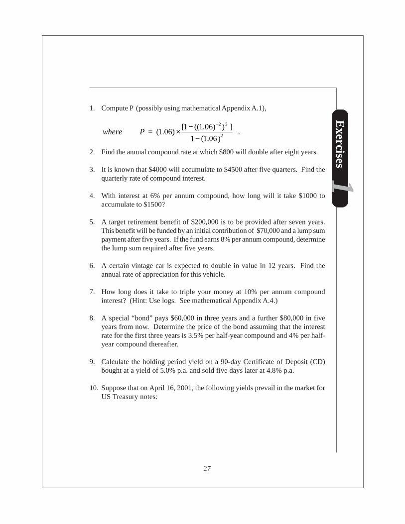
11. Compute P (possibly using mathematical Appendix A.1),
.
= P where
)06.1(1
]))06.1((1[)06.1(
2
32
−−×
−
2. Find the annual compound rate at which $800 will double after eight years.
3. It is known that $4000 will accumulate to $4500 after five quarters. Find thequarterly rate of compound interest.
4. With interest at 6% per annum compound, how long will it take $1000 toaccumulate to $1500?
5. A target retirement benefit of $200,000 is to be provided after seven years.This benefit will be funded by an initial contribution of $70,000 and a lump sumpayment after five years. If the fund earns 8% per annum compound, determinethe lump sum required after five years.
6. A certain vintage car is expected to double in value in 12 years. Find theannual rate of appreciation for this vehicle.
7. How long does it take to triple your money at 10% per annum compoundinterest? (Hint: Use logs. See mathematical Appendix A.4.)
8. A special “bond” pays $60,000 in three years and a further $80,000 in fiveyears from now. Determine the price of the bond assuming that the interestrate for the first three years is 3.5% per half-year compound and 4% per half-year compound thereafter.
9. Calculate the holding period yield on a 90-day Certificate of Deposit (CD)bought at a yield of 5.0% p.a. and sold five days later at 4.8% p.a.
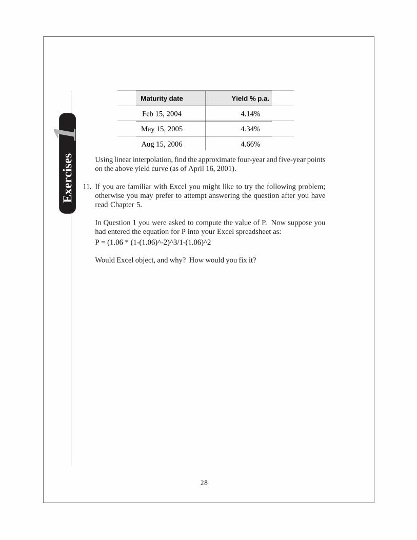
10. Suppose that on April 16, 2001, the following yields prevail in the market forUS Treasury notes:
28
Exe
rcis
es 1
Maturity date Yield % p.a.
Feb 15, 2004 4.14%
May 15, 2005 4.34%
Aug 15, 2006 4.66%
Using linear interpolation, find the approximate four-year and five-year pointson the above yield curve (as of April 16, 2001).
11. If you are familiar with Excel you might like to try the following problem;otherwise you may prefer to attempt answering the question after you haveread Chapter 5.
In Question 1 you were asked to compute the value of P. Now suppose youhad entered the equation for P into your Excel spreadsheet as:
P = (1.06 * (1-(1.06)^-2)^3/1-(1.06)^2
Would Excel object, and why? How would you fix it?

29

30

TwoTwoTwoTwoTwoThe Valuation of Cash Flows
31
In the last chapter, we saw that T-Bills and other similar financial instruments aresingle-payment securities. Many financial instruments are not single paymentsbut are a series of extended payments, so we need to modify our valuation conceptto include multiple payments. Coupon bonds are a good example of such a series,typically paying a cash flow (coupon) every six months and at the end, the return ofthe original capital. Thus part of this and other chapters will look at the tradingconventions and pricing for bonds. We shall also discover that bonds come in allvarieties, and that they can be priced in terms of competing versions of whatconstitutes an interest rate.
The second part of the chapter shifts the perspective somewhat. Valuing one bondis straightforward enough, once you have decided on the right way to do it. Butwhat about valuing a portfolio of bonds, or controlling the risk of a portfolio againstchanges in general interest rates? We look at some of the basic tools for doingthis, and in particular, the concept of duration, a sensitivity measure used by fixed-interest analysts and managers.
In this chapter we will also consider some of the instruments used in the managementof interest rate risk, including T-Bill, Eurodollar and Bond futures contracts.Derivatives of this kind can also be used for open position taking, i.e. speculation.We will look at the terminology, market trading conventions, and pricing.

Part I. Interest Rates and Foreign Exchange
32
Financial Modeling for Managers
2.1 Notation and definitions
Annuity A series of equal cash flows occurring at equal time intervals. Thereare two types of annuities. An ordinary annuity (or deferred annuity)pays cash flows at the end of the period (sometimes referred to aspaying in arrears). An annuity due pays cash flows at the beginning ofthe period.
a In fractional discounting, number of days from settlement date to thenext interest date.
b Number of days from last interest date to next interest date (i.e. totalnumber of days in the current interest period).
c Annual coupon rate, expressed as a decimal.
C The coupon payment (FV × c/2 for a bi-annual coupon).
D Macaulay duration: a weighted average of the times to receipt of aspecified group of cash flows, the weight being proportional to theirpresent values.
Derivative An instrument whose price is tied in some way or derived from,the price or yield of another instrument (the underlying ‘physical’).
EAR Effective annual interest rate. The true annual rate where a givennominal rate is compounded more than once inside a year.
FV Nominal or face value of the bond.
it
The effective interest rate for the period ended at time t, expressed asa decimal. The subscript, t, is omitted if the interest rate is constanteach period. In this case, i is the effective rate per period. (As we willsee later, this will be equal to r
m /m.)
rm
The nominal annual interest rate (APR) compounded m periods duringthe year.
r1
Effective rate per annum. The interest rate that would produce thesame ending value, as would have resulted if annual compounding hadbeen used in the first place.

33
Chapter Two. The Valuation of Cash Flows
n The number of compounding periods. In the case of an annuity, thenumber of cash flows. In the case of a coupon bond, the number ofcoupons remaining until maturity.
P Market value or price of the bond.
PQ
“Quoted” price, as distinct from invoice price, of a bond.
PVi
The present value of the ith payment.
PVIFi,n
Present value interest factor. This is equal to )1(
1ni +
or = (1 + i)-n.
PVIFAi,n
Present value interest factor for an annuity. This is equal to
i
i + n)1(
11−
.
PVA The present value of an ordinary annuity. The letter “A” is added todistinguish the present value of an annuity from other present values.
PVA= C× PVIFAi,n.
PVAD
The present value of an annuity due. The subscript “D” is added todistinguish the present value of an annuity due from ordinary annuities.
PVAD = C× PVIFAi,n × (1+i) .
ti
The time at which the ith payment is made or received.
IRR Internal rate of return, or the yield to maturity. This is the rate ofdiscount that equates the price (cost) of a bond or bill to the presentvalue of the cash flows—the coupons and the face value payment.
Forward A forward contract is an agreement calling for future delivery of anasset at a price agreed upon at the inception of the contract.
Futures A futures contract is a forward contract where the asset is instandardized units, quality and quantity, and which is marked to market(valued) every day until maturity. Futures contracts are traded onexchanges while forward contracts are over the counter instruments –that is, not exchange-traded.
Invoice versus quoted priceFor a bond, in some markets including the US, the invoice price is
Part I. Interest Rates and Foreign Exchange
34
Financial Modeling for Managers
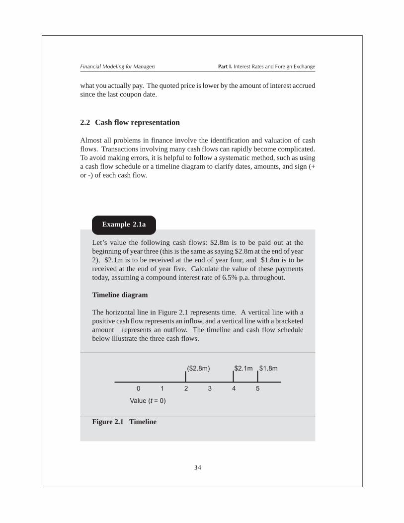
Let’s value the following cash flows: $2.8m is to be paid out at thebeginning of year three (this is the same as saying $2.8m at the end of year2), $2.1m is to be received at the end of year four, and $1.8m is to bereceived at the end of year five. Calculate the value of these paymentstoday, assuming a compound interest rate of 6.5% p.a. throughout.
Timeline diagram
The horizontal line in Figure 2.1 represents time. A vertical line with apositive cash flow represents an inflow, and a vertical line with a bracketedamount represents an outflow. The timeline and cash flow schedulebelow illustrate the three cash flows.
� � � � � �
����� ���� ���
������������
Figure 2.1 Timeline
Example 2.1a
what you actually pay. The quoted price is lower by the amount of interest accruedsince the last coupon date.
2.2 Cash flow representation
Almost all problems in finance involve the identification and valuation of cashflows. Transactions involving many cash flows can rapidly become complicated.To avoid making errors, it is helpful to follow a systematic method, such as usinga cash flow schedule or a timeline diagram to clarify dates, amounts, and sign (+or -) of each cash flow.

35
Chapter Two. The Valuation of Cash Flows
Cash flow schedule
Cash flow
Time (Years) 0 1 2 3 4 5
Cash flow
($m)
0.00 0.00 -2.80 0.00 2.10 1.80
At the left is a schedule of the timing and amounts of the cash flows. Inflows are expressed as positive numbers and outflows are expressed as negative numbers. Additional columns could be used to identify the sources and destinations of cash flows. This layout is similar to the way you would set up the problem in a spreadsheet.
Knowing the size, sign and timing of the cash flows, we can proceed withvaluing them. Formula (8) from Chapter 1 will be used to solve for thepresent value of each cash flow. The present values for the three cashflows will then be added together and this sum constitutes the presentvalue of the set of cash flows.
PV = $ -2.8(1.065)-2 + 2.1(1.065)-4 + 1.8(1.065)-5 = $ 477,518
Calculate the accumulated value of the cash flows in Example 2.1a attime t = 3.5 years (that is, halfway through the fourth year) again, assuminga compound interest rate of 6.5% p.a.
The value halfway through the fourth year is equal to:
Value3.5 = PV×(1.065)3.5 = 477,518×(1.065)3.5 = $595,269.16
Example 2.1b
By definition, the present value of a set of cash flows is simply the sum of thepresent values of the individual cash flows. When everything is valued to the samepoint in time, you are comparing apples with apples. At times, it may be necessaryto value cash flows to a point in time other than the present, that is, to a point in timeother than t = 0. The following example illustrates the valuation of a set of cashflows to a future point in time.

Part I. Interest Rates and Foreign Exchange
36
Financial Modeling for Managers
2.3 Valuing annuities
Many situations arise in practice where a series of equal cash flows occur at regularequal time intervals. Such a series of payments is called an annuity. Annuities arevery common. Examples include lease payments, insurance premiums, loanrepayments, and fixed interest coupons. When a set of cash flows does form anannuity, calculating the present value is relatively easy. As we shall see, it is nolonger necessary to value each flow separately.
The present value of an ordinary annuity
In an ordinary annuity, the cash flows fall at the end of each period.Consider a series of $1 payments at the end of each year for five years at6% p.a. compounded. Using the definition for the present value of a set ofcash flows, we would do the following calculations:
PVA = $1(1.06)-1 + $1(1.06)-2 + $1(1.06)-3 + $1(1.06)-4 + $1(1.06)-5
= $1(0.9434 + 0.8900 + 0.83962 + 0.79209 + 0.74726)= $ 4.21236
Thus, for an investment (loan) of $ 4.21, at 6.0% you would receive (pay)$1 per year for five years at the end of the period (in arrears).
Example 2.2
Notice that for an ordinary annuity, the cash flows are such that when we calculatethe present value, all cash flows are brought back (discounted) to one period beforethe first cash flow is received (or paid out). When we discuss the present value ofan annuity due, this will not be the case and will necessitate an amendment to theannuity formula.
Ordinary Annuity Formula
To illustrate how the formula is derived, consider Example 2.2 above, except thatwe shall remain a bit more general with an arbitrary interest rate i.

37
Chapter Two. The Valuation of Cash Flows
PVA = $1[(1+ i)-1 + (1+ i)-2 + (1+ i)-3 + (1+ i)-4 + (1 + i)-5].
Multiply both sides of the equation by (1+ i), and we get:
PVA (1 + i) = $1[ 1 + (1+ i)-1 + (1+ i)-2 + (1+ i)-3 + (1+ i)-4].
Subtracting the first equation from the second , PVA(1 + i) – PVA:
[ ]5)1(11$)1( −+−×=−+ iPVAiPVA
That is:
( )
+−×=×
51
111$
iPVAi
Then the present value formula for a five-period ordinary annuity where the cashflow is $1 is given by:
( )
+−
×=i
iPVA
51
11
1$
Using the same methodology, we can solve for the present value of any n-periodordinary annuity with cash flow C and interest rate i using the following formula:
( )
+−
×=i
iCPVA
n1
11
(1)
The term in brackets is written as PVIFAi,n
, the present value interest factorfor an annuity.

Part I. Interest Rates and Foreign Exchange
38
Financial Modeling for Managers
How much money would you be able to borrow if you had to repay theloan in 20 years with equal annual payments at an interest rate of 10.5%,if the most you could afford in annual payments is $3,000? Assume thefirst payment is in one year’s time.
( )
+−
×=105.0
105.01
11
000,3$ 20
PVA
PVA = $3,000 × [8.2309089] = $24,629.73
Example 2.3
Present value of an annuity due
In an annuity due, payments are made in advance rather than in arrears. Let usrevisit Example 2.2, but move the cash flows to the beginning of the period (or inadvance).
Using the definition for the present value of a set of cash flows, we woulddo the following calculations:
PVAD
= $1(1.06)0 + $1(1.06)-1 + $1(1.06)-2 + $1(1.06)-3 + $1(1.06)-4
= $1(1+ 0.9434 + 0.8900 + 0.83962 + 0.79209)= $ 4.46511
Thus for an investment (loan) of $ 4.47, you would receive (pay)immediately $1 per year for five years, at 6%. Notice that this amount is1.06 times larger than the $4.21 we got when we solved this problem before.This is no coincidence. If you compare the above calculation with the onefor the ordinary annuity, you will notice that the there is one less discountingperiod for every cash flow. We could take the first set of calculations (forthe ordinary annuity) and turn it into the annuity due calculations by multiplyingeach cash flow by (1 + i).
(1+ i) PVA = PVAD
Example 2.4

39
Chapter Two. The Valuation of Cash Flows
You will notice that for an annuity due, the cash flows are such that when wecalculate the present value all cash flows are brought back (discounted) to whenthe first cash flow is received (or paid out). Remember that for the present valueof an ordinary annuity, this is not the case.
Annuity due formula
As indicated above, we could replicate the argument used to derive Equation (1),but the only difference would be that all of the terms would be multiplied by (1+i).The resulting formula is:
PVAD = ( )ii
i + C
n
=×
−× 1
)1(
11
(2)
Be careful when working with annuity problems. The time period to which thecash flows are discounted determines whether you solve the problem with Formula(1) or (2). If all of the cash flows are discounted to one period before the first cashflow, use Formula (1). If all of the cash flows are discounted to when the first cashflow occurs, use Formula (2).
2.4 Quotation of interest rates
Interest rates tend to be quoted in many different ways, which sometimes makescomparison between quotes a problem. As we saw in Chapter 1 this was one ofthe reasons Congress passed the Consumer Credit Protection Act of 1968. Eventhough we discussed this topic briefly in Chapter 1, a little more detail is necessary.
Compound interest is calculated at the end of each interest period and compoundedinto (added to) the principal. The number of times interest is compounded in oneyear is called the compounding frequency per annum. The period of time betweensuccessive compounding is called the interest period.
Nominal (APR) and effective rates of interest
If $10,000 is invested at a nominal rate of 12% per annum with monthlycompounding, the effective monthly return is 1% compound and the effective annual

Part I. Interest Rates and Foreign Exchange
40
Financial Modeling for Managers
return is significantly higher than 12%. For at the end of 12 months, the $10,000would have grown at 1% compound per month to $10,000(1.01)12 = $11,268.25.If you look at the interest accumulation (by subtracting the principal of $10,000),you can see there is $1,268.25 of interest earned on a principal of $10,000. Thisrepresents an annual effective rate of 12.6825%. In other words, if you used a12.6825% p.a. interest rate compounded once during the year you would earn thesame as with the 12% compounded monthly in the above example.
This is the meaning of effective annual interest rate, EAR. We can see from Table2.1 below that as compounding frequency is increased, keeping the nominal rateconstant, the effective rate increases.
Table 2.1 Compounding frequency and effective rates
Compounding
Frequency
Nominal Rate %
p.a. (APR)
Effective Annual Rate %
Annually
6.00
6.00
Semi-annually
6.00
6.09
Quarterly
6.00
6.13636
Monthly
6.00
6.16778
Daily
6.00
6.18315
Continuous
6.00
6.18365
Up to this point, we have used the letter i in equations to denote the relevantperiodic interest rate. We have used such interest rates in a relatively general way,but now we are going to be more specific and introduce subscripts, so it becomesmuch clearer to switch to the letter r.
Consider $1 invested for a year at the nominal rate of rm. This means that the
interest compounds m times a year, and that the effective rate per compoundingperiod when there are m periods per year is r
m /m.
By the end of the year, the investment will accumulate to $1(1 + rm
/m)m. Thisrepresents the original $1 invested plus interest of (1 + r
m /m)m - 1. Thus, the
nominal rate of rm is equivalent to an annual effective rate of (1 + r
m /m)m - 1.

41
Chapter Two. The Valuation of Cash Flows
Consistent with this notation, define r1 as the effective rate from only one
compounding during the year (in other words, just the effective annual rate). Wesee that r
1 and r
m are related by the following formula:
(1 + r1 ) = (1 + r
m /m)m (3)
so that:
r1 = (1 + r
m /m)m - 1 (4)
Let’s take a moment and look at Equations (3) and (4). The left hand side ofEquation (3) is a one year future value interest factor using the effective annualrate; the right hand side is the one year future value interest factor using the nominalrate with an adjustment for the number of compounding (conversion) periods.
Notice also that Equation (4) above gives the same result as Equation (1) fromChapter 1 because r
m /m is equal to i, the periodic rate. Thus, the introduction of
rm
/m formalizes the way in which we calculate the periodic rate introduced inChapter 1.
Find the effective annual rate of interest corresponding to 6% (nominal)p.a. compounded (convertible) quarterly.
Here, rm
= 6% p.a. , and m = 4
Hence from Formula (4), r1
= (1 + .06 / 4)4 - 1
= 1.0613636 - 1 = 6.136%
As an exercise, you can now check the entries in Table 2.1 above, exceptfor continuous compounding which we will discuss in Section 2.5.
Example 2.5
Sometimes it is necessary to work backwards from the effective annual rate ofreturn to find the nominal rate. The next example will show us how to accomplishthis.

Part I. Interest Rates and Foreign Exchange
42
Financial Modeling for Managers
What nominal rate compounded every month will equate with an effectiveannual rate of 6.16778%? In other words, solve for r
m, where m = 12.
From expression (3) above: (1 + r1 ) = ( 1 + r
m /m)m
Hence (1 + r1 )1/m = ( 1 + r
m /m)
(1 + r1 )1/m - 1 = r
m /m
m((1 + r1 )1/m - 1) = r
m
So that, rm = m((1 + r
1 )1/m - 1)
In our case: r12
= 12 ((1 + .0616778 )1/12 - 1)
= 6% p.a. nominal compounding monthly
Of course you probably already knew the answer. Look at Table 2.1 again.This is just the monthly compounding number.
Example 2.6
It is market practice to express interest rates as nominal rates per annum. Howeverthe nominal rate is strictly meaningless, unless the compounding frequency isspecified, or understood. Likewise, specification of the interest period is essentialwhen speaking of effective interest rates.
Equivalent rates
Now we introduce a way to convert from one nominal rate, with a specified numberof compounding periods in a year, to another nominal rate, with a different numberof compounding periods, when they have the same equivalent annual effectiverate. We will differentiate between two nominal rates by using r
m to represent one
and rk to represent another.
Using (3) again: (1 + r1 ) = (1 + r
m /m)m , and (1 + r
1 ) = ( 1 + r
k /k)k
so (1 + rm /m)m = ( 1 + r
k /k)k
from which rm
= m((1 + rk /k)k/m - 1) (5)

43
Chapter Two. The Valuation of Cash Flows
From Formula (4), we know that the effective rate for 5% nominal p.a.compounded monthly is 5.11619% = r
1 = ((1 + .05
/12)12 - 1) × 100%.
What is the nominal rate compounded quarterly that has the same effectiverate?
Using expression (5), we get:
r4
= 4((1 + .05/12)12/4 - 1) × 100% = 5.02086%
The answer is 5.02086% nominal compounded quarterly. To check thisresult, try using Formula (4) and compute the effective rate. If the effectiverate is the same as above, you have the correct answer.
r1 = (1 + .050286
/4)4 - 1 = .0511619 or 5.11619%
The effective rates are the same, so 5% nominal p.a. compounded monthlyis equal to 5.02086% nominal p.a. compounded quarterly.
Example 2.7
Some guidelines on cash flow valuation and effective return:
1. The effective return must match the cash flow frequency
When valuing cash flows, remember to match the effective rateper period with the frequency of the cash flows. So, for example,if cash is rolling over monthly, an effective monthly rate should beused for valuation purposes.
2. When the investment or borrowing period is less than one year,adjust the effective return to an annual basis for comparisonpurposes.
Applying this formula to different nominal rates that do not have the same equivalentannual effective rate will give you nonsense.

Part I. Interest Rates and Foreign Exchange
44
Financial Modeling for Managers
Suppose that interest is paid at a nominal rate of 8% p.a. every 90 days.This investment rolls over so that interest is earned on the interest. Assumethat it compounds at the same rate for three periods of 90 days each. Whatis the effective annual return for the investment?
The effective 90 day rate is = 8% × 90 / 365
= 1 .9726027%
= .019726027 expressed as a decimal
Compounded for three periods of 90 days at the same rate, the effectiverate becomes:
= (1.019726027)3
= 1.0603531
That is, the effective return over the 270 days is:
= (1.0603531 - 1) × 100 = 6.0353%
As the investment does not benefit from another compounding period, tofind the effective annual rate, simply perform a pro-rata adjustment to 365days.
Effective annual rate = 6.03531 × 365 / 270 = 8.1588457%
Example 2.8
2.5 Continuous time compounding and discounting
Go back to the discussion in Section 2.4 and look at Table 2.1 again. You will noticethat as the compounding interval gets smaller, the effective annual rate tends to alimit, which is provided by continuous compounding. This means that there are aninfinite number of infinitesimally small compounding periods within the year.
You will recall from Formula (3) or (4) that if there are m compounding intervalsinside a year, then the annual effective compounding factor is

45
Chapter Two. The Valuation of Cash Flows
(1 + r/m )m,
where we have written the nominal annual rate as r. To simplify the discussion,we have dropped the subscript m, which is implied in the rate, r. In fact, in whatfollows we are going to keep the rate r constant as the compounding period mvaries, just as we did in Table 2.1. Of course, the basic unit of time here could beanything we please, but the usual practice is to normalize the time unit as one year.We already know that the effective interest rate
is higher than the nominal annual
rate r, and how much greater depends upon the compounding frequency (m).
Now, what happens as the compounding intervals diminish: down to amonth, then a week, then a day, an hour and so forth? Or equivalently,the number of intervals m grows larger and larger? There is a mathemati-cal result that says:
.e = m
r + rm
m)1(limit
∞→
Here the number e is the base for natural logarithms, one of the most importantconstants in mathematics. It is approximately equal to 2.71828. Most calculatorsand all financial calculators have an ex key which raises e to the xth power, and alsocan calculate its reverse: if y = ex, then x = ln (y), where the symbol ln denotes thenatural logarithm.
As you reduce the length of the time compounding interval, you are approachingcontinuous time where you have an infinite number of infinitesimally small timeunits. So the math is telling us that the continuous time compounding factor is equalto er, where r is the nominal annual rate, as m tends to infinity.
For the nominal annual rate of 12%, you would raise e to the 0.12 power, e0.12, andget 1.127497. Subtracting one (1) from this number as in Equation (4) and convertingto a percentage, you get the effective annual rate as 12.7497%, the last number inTable 2.1.
What about future values? Recall Equation (7) of Chapter 1, which says that:
FV = P0 × (1 + i)t ,
where t is the number of complete years.

Part I. Interest Rates and Foreign Exchange
46
Financial Modeling for Managers
Similarly, the present value formula (Equation (8) in Chapter 1) becomes:
PV = P0 = FV × e-rt (8)
Hence, the exponential function assumes the role of the continuous timecompounding or discounting factor. The astute reader will notice that since Chapter1, we have changed n to t. The change is necessary because of the convention ofusing t in continuous time problems.
Equations (7) and (8) are functions of t. Equation (7) has another usefulinterpretation. To develop it, we shall need a bit of differential calculus (if yourmath does not extend this far, skip the derivation and just note the final result).
Differentiating Equation (7) and using [ ] rtrt reedt
d = , we get:
rterPdt
dFV0=
= rFV , using (7) again.
This can be written:
.rFVdt
dFV
=
This equation illustrates that the instantaneous proportional rate of change of one’scapital is equal to the nominal rate, r. Or you could say the proportional change isequal to the nominal rate times the small time interval dt. Our capital is growingat an instantaneous rate of r %.
Much of advanced theory in finance is cast in terms of continuous time. There isasaying among mathematicians: “God made the integers, but man made thecontinuous.” If so, man certainly made things easier for himself, because the
If we have more than one compounding period in a year, substitute rm for i to
denote the nominal rate. The formula becomes:
FV = P0 × (1 + rm /m)) tm (6)
Equation (6) is the lump sum future value formula when there are m compoundingperiods in a year. Letting the units of time become infinitesimally small, and minfinitely large, changes Equation (6) to:
FV = P0 × ert (7)

47
Chapter Two. The Valuation of Cash Flows
mathematics of continuous time turn out to be much more powerful than that fordiscrete time. We will revisit this later when we discuss stochastic processes.
In the meantime, we note a more practical point. Once you get down to discretecompounding intervals like a day, it turns out that the difference between this andthe continuous time valuation is so small that people often choose the ease ofcontinuous time-based calculations.
2.6 Fixed interest securities
Coupon bonds
Coupon bonds are financial instruments that require the issuer to pay:
• A fixed amount, the face value (or principal), on the maturity or redemptiondate
• A number of periodic interest payments, known as coupons, of an amount thatis fixed at the time the bond is issued. It is usual for the coupon to be paidsemi-annually.
The market value of a bond should equal the present value of its future cash flows(where the cash flows consist of its face value and the periodic coupons) using thecurrent market yield.
For the discussion that follows, we will return to our original notation, using i todenote the effective interest rate per period.
The price of a coupon bond (P) is given by:
ni +
FV + C + ..... +
i +
C +
i +
C = P ,
)1(
)(2)1()1( (9)
where C stands for the coupon amounts and FV is the face value of the bond.
When calculating the price of a bond, it is assumed that the bond will be held tomaturity, and that the coupons will be reinvested at the current market yield tomaturity.
This assumption implies that we can rewrite Equation (9) as:
( ) ( ) ( ) FVCiCiCiP nnn ++++++=+ −−K
21 111 ,

Part I. Interest Rates and Foreign Exchange
48
Financial Modeling for Managers
meaning that a buyer of the bond should be able to achieve an accumulatedsum of P(1+i)n.In other words, you should be indifferent between accumulatingthe cost P, on the one hand, and the stream of rewards, on the other, all at thesame rate of interest, namely i.
For an investor, the above assumption results in a reinvestment risk. If interestrates fall and remain below the purchase market yield, the coupons will be reinvestedat a lower rate. Should the investor hold the bond to maturity under such aninterest rate scenario, the actual yield achieved by the investor will not match theyield implicit in the price at which the bond was purchased. If interest rates riseand remain above the purchase market yield, the coupons will be reinvested at ahigher rate and the actual yield will be higher.
In the United States the market tends to trade bonds on the basis of price. Given amarket price P, Equation (9) determines the effective rate per period (i) as theinternal rate of return (IRR) on the bond. This IRR is the per period rate whichequates the present value of the cash flows from the bond, including its repaymentof principal, with the market price, P. If the coupons are paid every six months theIRR will be a six-month rate and will need to be multiplied by two to annualize it.
In some other parts of the world, such as Australia and New Zealand, bonds tendto be bought and sold on the basis of market yield, which is quoted as a nominalannual rate. As the effective periodic rate, i, used in Equation (9) is usually semi-annual, you will need to take the quoted nominal annual rate and divide by two tocalculate price.
Readers familiar with corporate finance will know that the internal rate of returnof a project is the discount rate that equates the present value of the project cashflows with the upfront cost of the project. This is exactly the idea behind Equation(9), where the coupons and final principal payment correspond to the cash flowsand the given price of the bond to the upfront cost. In some circumstances involvingcash flows of alternating sign, there can be multiple different rates of return froma given set of cash flows, but this awkward property does not feature in bondpricing, where the rate is always unique. As mentioned above, the assumption inusing the internal rate of return is that it implicitly assumes that all coupons receivedare reinvested back into a financial instrument with exactly the same rate of returnas the bond. There is no reason this should automatically be true, and in mostcases it isn’t. Therefore, it can be hazardous to compute the yield from one bondand then use this yield to find the price for another. We’ll discuss this further in thenext chapter.

49
Chapter Two. The Valuation of Cash Flows
Using Formula (10) above, we can price a bond that has four years (eightsix-month periods) until maturity. Suppose the bond has a face value of$100 and pays semi-annual coupons of 12% p.a., and that the market yieldfor the bond is currently 12% p.a. (compounding semi-annually, i.e., 6%effective per six-months).
The semiannual coupon payments are: $100 × .12/2 = $6
Hence, on the basis of a notional $100 face value, the price of the bondwill be:
P = 6 × PVIFA.06,8 + + )06.1(
1008
=( )8
8
06.1
100
06.006.1
11
6 +
−×
= 37.2587629 + 62.7412371
= 100.00
Example 2.9
Note that in the bond markets, no $ sign would be associated with the above price.Bonds are normally issued in multiples of $1,000 for corporate bonds and $10,000for government bonds in the US. To keep things consistent, bond prices are
The above bond pricing Formula (9) is simple enough to apply if the number ofcoupon periods left to run is few, or if you have some time and a computer. However,using what we have learned about annuities (Section 2.2), we can take a shortcutin our calculations to find the present value of a coupon bond. The coupon paymentsvalued as an ordinary annuity, along with the present value of the lump sumrepayment of principal or face value, determine the total value of the bond. Thus,we can combine Equation (1) from this chapter and Equation (8) from Chapter 1,to get a closed form alternative.
P = C × PVIFAi,n + FV× PVIFi,n (10)

Part I. Interest Rates and Foreign Exchange
50
Financial Modeling for Managers
Suppose that the market yield is in fact 13% for the bond in Example 2.9.Assume the same 12% coupon and 4 years term left to maturity. Then theprice for the bond will be:
P = 6 × PVIFA8,.065 + + )065.1(
1008
)065.01(
100
065.
)065.1(16
8
8
+−×
−
+ =
= 36.5325058 + 60.4231188
= 96.9556245
Example 2.10
frequently calculated as a % of face value. Thus, the price means that the bondsells at that percentage of its face value. To convert to the dollar price, simplymultiply the FV of the bond by the price (% of its face value). Because of thevarious face values for bonds in the US, it is important to keep calculation to atleast seven decimal places for accuracy.
From the example above, we see that a bond priced on its coupon date at the sameyield as its own coupon, will be worth only its face value—no more and no less.
In this example, the price of the bond is given to seven decimal places. This isnecessary as the majority of such bonds are bought and sold in amounts of tenmillion or more.
When market yield increases above the coupon rate, the price of the bond will fallbelow its face value—the bond is said to sell at a discount. On the other hand, ifthe yield were 11% instead of 12%, the price would be 103.167 2830. Since thebond in this case is selling above its face value, it is said to be selling at a premium.This will occur whenever the market yield falls below the coupon rate.
Formulas (9) and (10) assume that the bond is valued with one full discountingperiod remaining before the first coupon is received, such that n is a whole number.What happens when n is not a whole number?
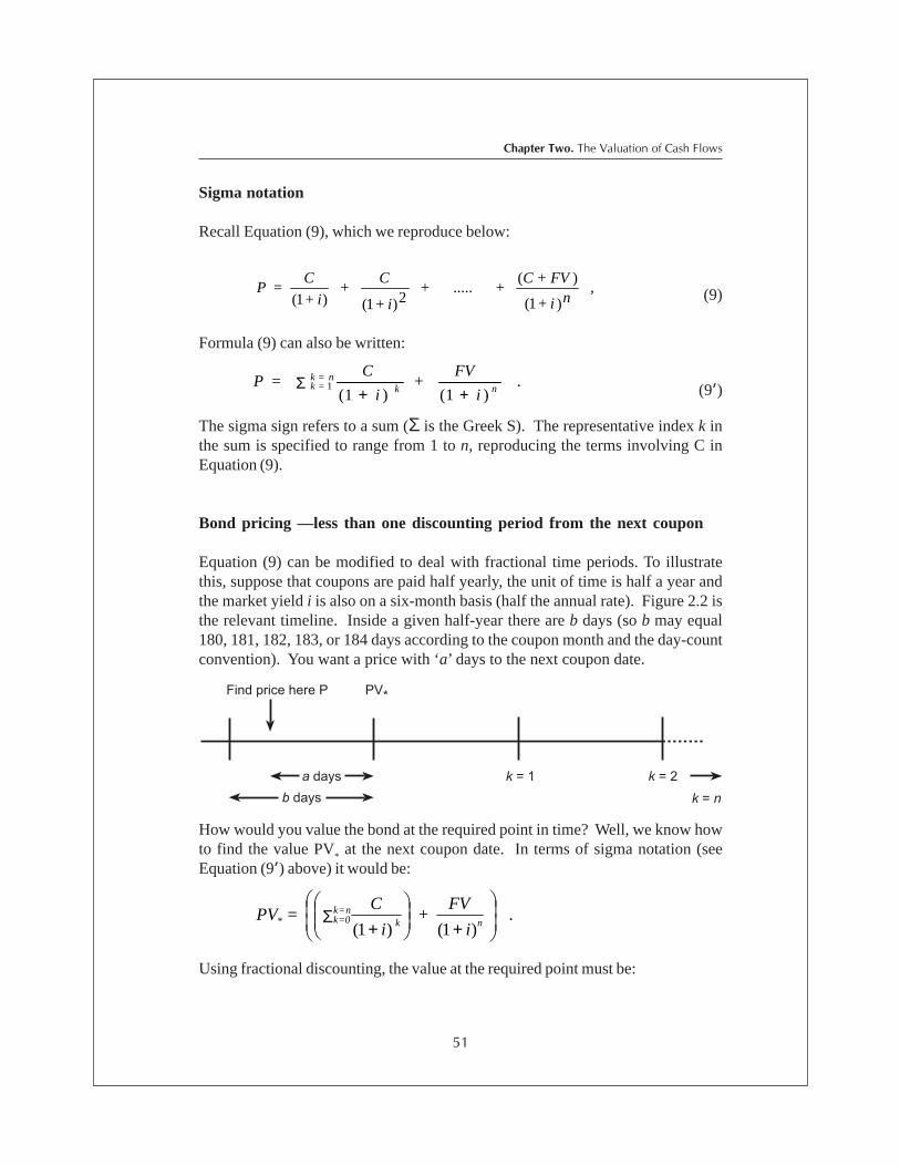
51
Chapter Two. The Valuation of Cash Flows
Formula (9) can also be written:
. i
FV +
i
C = P nk
n=k=k
)1()1(1
++Σ (9r)
The sigma sign refers to a sum (Σ is the Greek S). The representative index k inthe sum is specified to range from 1 to n, reproducing the terms involving C inEquation (9).
Bond pricing —less than one discounting period from the next coupon
Equation (9) can be modified to deal with fractional time periods. To illustratethis, suppose that coupons are paid half yearly, the unit of time is half a year andthe market yield i is also on a six-month basis (half the annual rate). Figure 2.2 isthe relevant timeline. Inside a given half-year there are b days (so b may equal180, 181, 182, 183, or 184 days according to the coupon month and the day-countconvention). You want a price with ‘a’ days to the next coupon date.
�����
�����������������
�����
�����
������
������
� �
How would you value the bond at the required point in time? Well, we know howto find the value PV
* at the next coupon date. In terms of sigma notation (see
Equation (9r) above) it would be:
. i
FV +
i
C = PV
nk n=k
=0k
+
+Σ
)1()1(*
Using fractional discounting, the value at the required point must be:
Sigma notation
Recall Equation (9), which we reproduce below:
ni +
FV + C + ..... +
i +
C +
i +
C = P ,
)1(
)(2)1()1( (9)

Part I. Interest Rates and Foreign Exchange
52
Financial Modeling for Managers
Combining the two steps, this turns out to be same as writing:
,)1()1(
i
FV +
i
C = P
n + b
ak +
b
an=k
=0k
+
+Σ (11)
which is the general formula for the bond price with fractional discounting.
Fractional discounting assumes that the periodic interest rate applies to the fractionaltime period. Be careful when using fractional discounting—it’s only valid whenthe financial contract stipulates it in writing, or when market participants use it byconvention. In the case of bond pricing, markets adopt this form of fractionaldiscounting by convention.
Here’s an additional wrinkle. There are two prices for bonds that sell in the UnitedStates (and other countries): the invoice price and the quoted price. The invoiceprice is the P from Equation (11). This is the total that you will pay for the bond.The quoted price will be lower by the amount of interest that has accrued since thelast coupon payment. This interest amount is not a compounded amount, which iswhat we are doing in Equation (11), but is a simple interest amount. Mixing twointerest payment systems— simple and compounding—is a curiosity of bond mathwhich tends to be a challenge for the novice price maker.
The quoted price formula is,
−×−
++Σ
b
aC
i
FV +
i
C = P
n + b
ak +
b
an=k0=kQ 1
)1()1( (12)
Transforming Equation (11) into a closed form gives us:
[ ] [ ] .)1()1( ,,/
niniba PVIFFVPVIFACiP ×++××+= − (13)
Transforming Equation (12) into a closed form gives us,
[ ] [ ] . -1 C)1()1( ,,/
×−×++××+= −
b
aPVIFFVPVIFACiP nini
baQ (14)
( )*
1
1PV
iP
b
a×
+=

53
Chapter Two. The Valuation of Cash Flows
Find the invoice price for the March 31, 2003 US Treasury issue with acoupon rate of 4.25% p.a. The market yield is currently 4.283% andsettlement date is April 19, 2001. The semi-annual coupons are $2.125 per$100 face value (C = 4.25). The number of full coupon periods left to runis three (n = 3, from September 30, 2001 to March 31, 2003). The numberof days from settlement date to the next interest date is 164 days (a =164). The number of days from the last interest date, March 31, 2001, tothe next interest date, September 30, 2001, is 183 days (b = 183). Thecurrent market yield is 2.1415% per half year (i = 0.021415).
We will use Equation (13) for pricing the bond. Per $100 face value, thebond will price at:
( ) ( )[ ]93841151008759532112520214151 183
164
.... ×++××
+=−
P
= 0.9811902 × [102.0775468]
= 100.1574861
This determines the total amount to be paid for the bond – the invoiceamount.
The quoted price per $100 face value is the invoice price less the accruedinterest. The term we have to subtract is:
22062840183
164112521 .. =
−×=
−×b
aC
Hence, the quoted price per $100 face value is:
100.1574861- 0.2206284 = 99.9368577 ≅ 99.94
Example 2.11
To make matters worse, a and b are not the same for all bonds. For US federalagency and corporate bonds, a is calculated using a thirty day month and b is basedon a 360 day year (180 day half year). For US Treasuries, a is the actual numberof days from settlement date to the next interest date, and b is the actual number ofdays between coupons.

Part I. Interest Rates and Foreign Exchange
54
Financial Modeling for Managers
Zero-Coupon Bonds
Zero-coupon bonds consist of just a single cash flow, paid at the bond’s maturitydate. There are no intervening coupons. In the US, taxes are computed on capitalgain as well as ordinary income. This places zero-coupon bonds at a psychologicaldisadvantage to coupon bonds. People do not like paying taxes on something fromwhich they aren’t earning income. This is why zeros are popular in IRAs and othertax advantaged accounts. In some countries where tax is assessed on a cash flowbasis, these zeros enjoy a considerable tax advantage. In addition, zero couponbonds have considerable theoretical importance in finance.
In general, zero coupon bonds:
• have an initial term of greater than 1 year• have no intermediate cash flows• are always purchased below face value• usually have six-month compounding.
The zero pricing equation is:
P = r
FV
n.
21
+ (15)
where r = the nominal annual zero-coupon rate expressed as a decimaland n = the number of half-years to maturity.
Price a ten year zero-coupon bond with face value $1m at a market yieldof 7% p.a. Assume the usual semi-annual compounding.
. 8$502,565.8 =
2
07. + 1
$1,000,000 =
20
P
If the market yield increases to 8%, the bond re-prices to:
Example 2.12

55
Chapter Two. The Valuation of Cash Flows
=
+
= P .95.386,456$
208.
1
000,000,1$20
The bondholder will incur a capital loss of $46,178.93, a very significant“hit” for an initial investment of $502,565.88. We can express this as apercentage loss:
.%18863.9%10088.565,502$
93.178,46$ = ×
Note that this capital loss will not be realized until the holder sells the bond.It does, however, represent the opportunity cost of holding the instrument.
The problem of potential capital loss is an extremely important one forthose who hold investments or issue liabilities, so it is worthwhile to comparethe sensitivity of such an instrument to that of other financial instruments.Such information will be highly useful to portfolio managers making decisionsabout purchases and sales (or issues and buy backs) of assets (liabilities)given various expected interest rate changes.
To illustrate this, consider a much shorter-term security, for example, adiscount instrument such as a CD, and evaluate the change in its valuegiven a change in interest rates.
Price a 90 day CD with a face value $1m when the market yield is 7%.Recall that we can price this security directly using Formula (4) from Chapter1, because CDs are priced using the bond equivalent approach:
n
i +
FV = Price .
3651
×
Example 2.13

Part I. Interest Rates and Foreign Exchange
56
Financial Modeling for Managers
where:
FV = face or nominal value of the securityn = number of days from settlement date to maturityi = (nominal annual) yield for securities of n days to maturity.
Given the numbers quoted above, we have:
. =
+
= Price 59.032,983$
365
9007.01
000,000,1$
×
Now, suppose that the instant after you bought it, the market re-prices the90-day CD yield at 8% p.a. The new price is:
. =
+
= Price 56.655,980$
365
9008.01
000,000,1$
×
If you decide to sell with 90 days still to run, you will record a capital lossof $2,377.03. On the other hand, if the CD is held to maturity you will earn7% instead of 8%, which could have been earned had the purchase beenbetter timed. You have incurred an opportunity loss of 1%.
Expressing this capital loss as a percentage:
.%241806.0%10059.032,983$
03.377,2$ = ×
In summary, when interest rates move from 7% to 8%, there is a capitalloss of 0.24%.
Clearly this instrument is far less price sensitive to changes in the interest rate thana much longer term instrument such as the ten-year zero coupon bond in Example2.10, where the capital loss was 9.2%. The issue of value sensitivity is going to beimportant for fixed interest managers, and we take this up in the next section.
57
Chapter Two. The Valuation of Cash Flows
2.7 Duration and value sensitivity
While the concept of duration is commonly applied to bonds and other tradedfixed interest instruments, it can be applied to any set of cash flows. Duration is ameasure of the average weighted times to receipt for a given set of cash flows.
For example, suppose we are to receive $1000 in one month plus $1000 in threemonth’s time. We could say that on average we are to receive $2000 in two months.The simple average term of this cash flow would be approximately two months.
Duration is measured however, not as the simple average of the timing of payments(as for the cash flows above), but as a weighted average of the timing of paymentswhere the weights are the present values of the cash flows. This makes allowancefor the time value of money.
Suppose we have a series of cash flows, accruing at times ti into the future, where
i ranges from i= 1 to i = n. In other words, cash flow #1 occurs at time t1, cash
flow #2 at time t2, and so on. Let cash flow #i have present value PV
i, and let PV.
ii
n
iPVt∑ =1 , be the total present value of the set of cash flows. Duration is
defined by:
∑
∑
=
==n
i i
ii
n
i
PV
PVtD
1
1
∑ =
= n
i
ii PV
PVt
1 (16)
Version (16) makes it clear that each time to receipt ti is weighted by its share of
the total PV generated.
In the case of a bond, PV = P, the bond’s market value, and the PVi refer to the cash
flows generated by the coupons and the final return of principal.
If the PV’s are calculated on a yield to maturity basis (as we have so far assumedin this chapter), the resulting D is called Macaulay duration. Another version,called Fisher Weil duration, utilizes zero coupon rates to calculate the PV
i (See
Chapter 3).

Part I. Interest Rates and Foreign Exchange
58
Financial Modeling for Managers
We will calculate Macaulay duration for a 10% coupon bond, which hastwo years left to run and a yield to maturity of 8.0%. Assume a face valueof $1m. We can use a spreadsheet to generate a table such as the one thatfollows.
Table 2.2 Calculation of Macaulay Duration for two-year bond
Time (ti)
Cash flow
Present Value PVi
ti * PVi
0.5
50,000
50,000 = 48,076.92 (1.04)
24,038.46
1.0
50,000
50,000 = 46,227.81 (1.04)2
46,227.81
1.5
50,000
50,000 = 44,449.82 (1.04)3
66,674.73
2.0
1,050,000
1,050,000 = 897,544.40 (1.04)4
1,795,088.80
Totals
PV = 1,036,298.95
1,932,029.80
To simplify the spreadsheet calculation, we have designated t in years sothat D is also expressed in years. (If we had calculated this using six-month periods, the result would have been twice as large, or 3.7287113six-month periods). We have:
D = 1,932,029.801,036,298.95
= 1.864 years
Note that the duration of the bond is less than its term to maturity, whichis two years.
In the case of a bond, Equation (16) has a closed form version.
D =ii nc
icni
i
i
+−+
−++−+
]1)1([
)()1(1 (17)
Example 2.14

59
Chapter Two. The Valuation of Cash Flows
Where: i = the effective interest rate for the periodc = the coupon rate for the period expressed as a decimaln = the number of compounding periods
Let’s continue with Example 2.14 by calculating the duration, using Formula(17).
D = 04.]1)04.1([05.
)04.05(.4)04.1(
04.
04.14 +−∗
−×++−+
= 26.0 - 22.2712887
= 3.7287 six month periods or 1.864 years
For a bond of maturity n periods, notice that if the coupon rate is equal to zero, theformula collapses to simply n. Therefore, the duration of a zero coupon bond issimply equal to its time to maturity.
Not quite as obvious is the closed form solution for the duration of an annuity.With a little more algebraic manipulation we can get the duration for an annuity ofn periods as equal to:
D = ]1)1[(
1
−+−+
ni
n
i
i (18)
Duration is employed in the measurement and management of interest rate risk.
Duration is used as a measure of the price sensitivity of an instrument (or that ofa portfolio of instruments) to changes in interest rates. This use results from therelationship between the instrument’s duration and the percentage change in theinstrument’s price caused by a change in interest rates.
We can describe the sensitivity relationship numerically as
.1
∆×≈∆i +
i D -
P
P(19)
where: ∆ represents a small changeP is the price of the instrumentD is the duration in interest periodsi is the (effective) period interest rate

Part I. Interest Rates and Foreign Exchange
60
Financial Modeling for Managers
The left-hand side of Equation (19) is the percentage change in the price of theinstrument. The right hand side of the equation indicates that D is approximatelythe coefficient of changes in the interest rate as they affect price. This equationfrequently appears in a slightly different form as:
i D - PP ∆×′≈∆
(19r)
where: D′ = D / (1+ i ) and is known as modified duration.
For Example 2.14 above we can calculate modified duration as:
years1.79periods5853
2080
1
72871133D ==
+=′ .
..
The interpretation is that a 100 basis point increase in the interest rate (for example,from i=10% to i=11%), will produce a capital loss of 1.79%.
Another use of duration is in the area of portfolio immunization. This approachallows the investor to eliminate exposure to interest rate risk by matching theduration of an investment portfolio to the required investment horizon.
To see how this works, suppose you had a commitment to pay $1 million in fiveyears time. You could buy a five-year zero coupon bond with a face value of $1million. Now suppose five years have passed and interest rates have changed.Would this affect your ability to meet the contract? Clearly not – your bond willpay exactly $ 1 million now and you are OK.
But would this be true if instead of a five-year zero coupon, you had bought—say—a ten-year coupon bond, intending to sell it after the five years? Supposethat near the end of the fifth year, interest rates had risen. Would you then be ableto meet your $1 million contract? This is doubtful, as the price of the bond wouldbe lower.
Instead, you can ensure that whatever bond or portfolio you use, its initial durationis set equal to the investment horizon (in this case, five years). This effectivelyturns your portfolio or coupon bond (in terms of interest rate dynamics) into an

61
Chapter Two. The Valuation of Cash Flows
equivalent zero coupon bond. You can make this exact by a small amount ofrebalancing as time passes, to keep the duration equal to the remaining investmenthorizon. For instance, you would occasionally need to swap the current investmentfor a coupon bond of slightly lower duration. But for most horizons, the rebalancingrequired is small.
2.8 Interest rate futures
Forward contracts are agreements calling for future delivery of an asset at a priceagreed upon at the inception of the contract. A futures contract is a more tradableform of a forward contract that is marked to market each day, with the change invalue being credited or debited to your account with a broker. To ensure tradability,futures contracts are written on underlying assets (physicals) of standardized units,quality and quantity. Futures contracts are traded on exchanges, while forwardcontracts are not—they are OTC (“over the counter”) instruments. In this chapter,we limit our discussion to interest rate futures contracts.
At least 30 interest rate futures contracts are traded on the Chicago Board of Trade(CBOT) and the Chicago Mercantile Exchange (CME). Summary listings of thesecontracts are provided in Tables 2.4 – 2.6 in the appendix to this chapter.
Futures are used for two main purposes—hedging and taking open positions(speculating). Some people need to reduce or eliminate price movements in theunderlying commodity. The mitigation of such natural exposures is known ashedging. Others try to profit from price movements in the underlying commodity.Because you need only put down between 5% and 15% margin, depending on thecontract, futures are heavily leveraged instruments favored amongst speculators.
The use of derivatives in risk management and speculation is beyond the scope ofthis book. However, we will look briefly at three examples of future contracts—the T-bill, the Eurodollar and T-bond contracts—which are used for the purposeof hedging interest rate risk.
U.S. T-Bill futures
The 13-week (three month) Treasury bill contract is based on a simple discountsecurity, the T-bill that was discussed in Section 1.3 of Chapter 1.

Part I. Interest Rates and Foreign Exchange
62
Financial Modeling for Managers
Table 2.3
Table 2.3 captures the “feel” of how 13-week T-bill futures would bepresented in the Wall Street Journal. The only difference is that therewould be nothing indicating that the yield is a discount yield – the WSJassumes that the reader knows this. The open, high, low and settlementprice are not “true” prices, but are another way of specifying the annualdiscount interest rate. A settle price of 93.64 means an annualized discountfrom par of 6.36% (100%-93.64% = 6.36%). This 6.36% is an annualrate based on 90 days and a 360-day year. Converting it to a 90-daydiscount yield is done by multiplying 90/360 by 6.36% = 1.59%.
If you buy this contract, the invoice price you are promising to pay is:
P =
×−×360
900636.1000,000,1$ = $984,100.00
Notice that P is not subscripted with a 0. The reason is that technically thistransaction will take place in the future at the contract expiration date,though most are closed out prior to this date at the market price quoted atthe time. The latter will be listed next to the T-bill contract in the WSJ. Fora complete listing of contract expiration dates and other information forcontracts traded at the Chicago Mercantile Exchange, go to http://www.cme.com/clearing/spex/XMLReports/intrRateGroup.htm.
What happens if the interest rate (discount) drops by one basis point to6.35%? The price for a new contract for will now be:
P =
×−×360
900635.1000,000,1$ = $984,125.00
Example 2.15
Open High Low Settle Change Open InterestYield Change
93.69 93.69 93.64 93.64 -0.09 6.36 0.09 221
Discount

63
Chapter Two. The Valuation of Cash Flows
Notice the difference between the original contract and the new one is$25.00, which is exactly two (half basis point) ticks for this contract (seeTable 2.4 in the appendix to this chapter).
If the interest rate rises by one basis point the price of a new contract willbe:
P =
×−×360
900637.1000,000,1$ = $984,075.00
This time the difference in value between the two contracts is -$25.00—once again, exactly two (half basis point) ticks. In each case, the gainsand losses will be posted to your broker account. Where current losseseat too much into the margin you have lodged with the broker, you will berequired to front up more cash to restore the margin.
To evaluate gains or losses when trading this contract, it isn’t actuallynecessary to go through all the calculations that we performed above. Wecan measure such gains and losses for the T-bill contract simply by
The Eurodollar time deposit contract
Another three-month contract trading on the CME—one that enjoys greaterpopularity and liquidity than the T-bill contract—is the Eurodollar Time Depositcontract. It has a principal value of $1,000,000 and trades in one-tick (= one basispoint) movements worth $25.00 per basis point for all but the current monthcontract, for which the contract trades in half-tick movements (= half basis point)worth $12.50 per half-tick. Like the T-bill contract, the Eurodollar contract isquoted using a price index, which is derived by subtracting the current interestrate for the contract from 100.00. For example, an interest rate of 4.50% translatesto a futures index price of 95.50 (100.00- 4.50 = 95.50).
To measure gains or losses on Eurodollar futures positions, the calculation is:
• Number of ticks moved × $25.00 × number of contracts held.
For the current month contract this calculation becomes:
• Number of half-ticks moved × $12.50 × number of contracts held.

Part I. Interest Rates and Foreign Exchange
64
Financial Modeling for Managers
In late June, a corporate treasurer reviewing his company’s cash flowprojections, estimates borrowing requirements of $10,000,000 for mid-September. The floating-rate bank loan the treasurer has negotiated willbe priced at one percent over the three-month Eurodollar LIBOR rate atthe time of funding (with interest paid quarterly). LIBOR is currentlyquoted at 5.35%, while September Eurodollar futures, which can be usedto lock in a September borrowing rate, are trading at 94.45, giving an impliedforward rate of 5.55% (calculated as 100.00- 94.45).
The corporate treasurer, concerned that rates will rise over the time periodprior to drawing down the loan, decides to “fix” the borrowing rate byselling ten Eurodollar contracts. Since the September Eurodollar contractwill trade very close to the three-month Eurodollar LIBOR rate by mid-September, the borrowing rate achieved by the treasurer will be very closeto 6.55% (the Eurodollar futures rate of 5.55% plus the bank’s 1% spreadover LIBOR).
The hedge works in the following way:
On June 29, the corporate treasurer sells ten Eurodollar futures contractsat 94.45 (i.e. a rate of 5.55%). Suppose that by September 15th, theEurodollar LIBOR physical rate has risen to 5.75%. The loan rate,including the bank’s margin, will be at 6.75%. However, if the corporatetreasurer is able to buy ten Eurodollar futures contracts at the same LIBORinterest rate (and it will be very close if not exactly the same), the futuresposition will be closed out at 94.25 for a gain of 20 basis points (94.45-94.25). The 20 basis points earned on the futures contracts will effectivelyreduce the cost of the loan from 6.75% to 6.55%.
Example 2.16
Eurodollar positions that are not closed out prior to settlement date are cash settledusing a final settlement price based upon the British Bankers Association (BBA)rate fixing. The rate that applies is the BBA Interest Settlement Rate for three-month U.S. dollar deposits determined at 11:00 a.m. London time on the contract’slast trading day. For Eurodollar contracts held until contract closeout, the finalsettlement price is rounded to four decimal places.

65
Chapter Two. The Valuation of Cash Flows
The 30-year T-bond futures
Let us briefly turn our attention to another popular interest rate futures contract—the 30-year Treasury bond. Because of the complexity of this contract, we willdescribe only its important features. If you are interested in more detail, visit theChicago Board of Trade (CBOT) website at: http://www.cbot.com.
The underlying instrument is a hypothetical 20-year 6% semi-annual coupon Treasurybond. The quote in the Wall Street Journal will be three digits followed by ahyphen and two more digits. For example, if you see 101-26 it means that thecontract is trading at 101 and 26/32’s of the $100,000 par value. This contract isnot a cash-settled contract. If you hold the instrument until maturity you mustdeliver (if you shorted the contract) or buy (if you are long the contract) one T-bond for every contract.
If you are the one who is delivering the bond, what happens if you can’t find a 20-year T-bond with a 6% semi-annual coupon? Fortunately, you can deliver a T-bondthat has a minimum of 15 years before the Treasury can call it. Suppose you havefound a 5% 20-year bond, which the CBOT has deemed acceptable for satisfyingthe contract. But the value of this bond is less than the value of the underlying bondof the futures contract. Receiving this would be unfair to the other party. On theother hand, if all you can find is a 7% 20-year bond that is more valuable now, thiswould be unfair to you. If these issues went unresolved there would be little demandfor these contracts.
To resolve these issues, the CBOT uses conversion factors. The conversion factor(CF) is calculated:
CF = ∑=
n
tt
tcashflow
1 03.1/100,000
Conversion factors are updated and published by the board of trade in Excel anddownloadable by going to http://www.cbot.com/cbot/docs/22879.xls. Thesefactors are constant throughout the trading period of the contract. The invoiceprice paid by the buyer of the Treasury bonds delivered to the seller is calculatedby the following equation:
Invoice price = contract size × futures contract × settlement price conversion factor

Part I. Interest Rates and Foreign Exchange
66
Financial Modeling for Managers
Suppose that the contract settles at 97-00, which is 97% of par. Theconversion factor for the bond being delivered is 1.05 (just downloadedfrom the CBOT website). Thus, the invoice price of the bond to be deliveredis:
$100,000 × .97 × 1.05 = $101,850
Example 2.17
There is much more to be said about the 30-year T-Bond futures contract andfutures contracts in general. The Chicago Board of Trade and the ChicagoMercantile have excellent websites with suggested reading for those who wish toexplore this area in more detail.
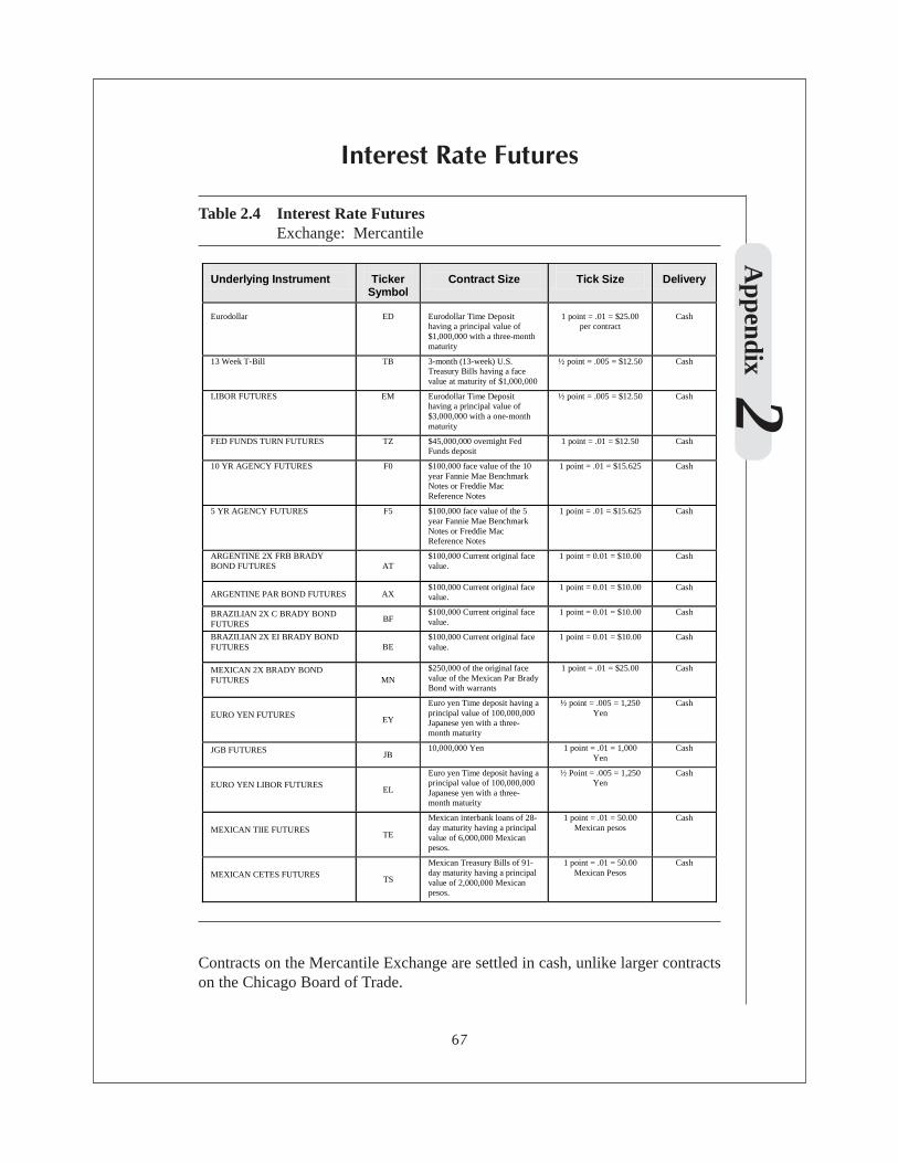
Interest Rate FuturesA
ppendix 2
67
Underlying Instrument
Ticker
Symbol
Contract Size
Tick Size
Delivery
Eurodollar
ED
Eurodollar Time Deposit having a principal value of $1,000,000 with a three-month maturity
1 point = .01 = $25.00
per contract
Cash
13 Week T-Bill TB 3-month (13-week) U.S. Treasury Bills having a face value at maturity of $1,000,000
½ point = .005 = $12.50 Cash
LIBOR FUTURES
EM Eurodollar Time Deposit having a principal value of $3,000,000 with a one-month maturity
½ point = .005 = $12.50 Cash
FED FUNDS TURN FUTURES
TZ $45,000,000 overnight Fed Funds deposit
1 point = .01 = $12.50 Cash
10 YR AGENCY FUTURES
F0 $100,000 face value of the 10 year Fannie Mae Benchmark Notes or Freddie Mac Reference Notes
1 point = .01 = $15.625 Cash
5 YR AGENCY FUTURES
F5 $100,000 face value of the 5 year Fannie Mae Benchmark Notes or Freddie Mac Reference Notes
1 point = .01 = $15.625 Cash
ARGENTINE 2X FRB BRADY BOND FUTURES
AT
$100,000 Current original face value.
1 point = 0.01 = $10.00 Cash
ARGENTINE PAR BOND FUTURES AX $100,000 Current original face value.
1 point = 0.01 = $10.00 Cash
BRAZILIAN 2X C BRADY BOND FUTURES
BF $100,000 Current original face value.
1 point = 0.01 = $10.00 Cash
BRAZILIAN 2X EI BRADY BOND FUTURES
BE
$100,000 Current original face value.
1 point = 0.01 = $10.00 Cash
MEXICAN 2X BRADY BOND FUTURES
MN
$250,000 of the original face value of the Mexican Par Brady Bond with warrants
1 point = .01 = $25.00 Cash
EURO YEN FUTURES
EY
Euro yen Time deposit having a principal value of 100,000,000 Japanese yen with a three-month maturity
½ point = .005 = 1,250 Yen
Cash
JGB FUTURES
JB 10,000,000 Yen 1 point = .01 = 1,000
Yen Cash
EURO YEN LIBOR FUTURES
EL
Euro yen Time deposit having a principal value of 100,000,000 Japanese yen with a three-month maturity
½ Point = .005 = 1,250 Yen
Cash
MEXICAN TIIE FUTURES
TE
Mexican interbank loans of 28-day maturity having a principal value of 6,000,000 Mexican pesos.
1 point = .01 = 50.00 Mexican pesos
Cash
MEXICAN CETES FUTURES
TS
Mexican Treasury Bills of 91-day maturity having a principal value of 2,000,000 Mexican pesos.
1 point = .01 = 50.00 Mexican Pesos
Cash
Table 2.4 Interest Rate FuturesExchange: Mercantile
Contracts on the Mercantile Exchange are settled in cash, unlike larger contractson the Chicago Board of Trade.
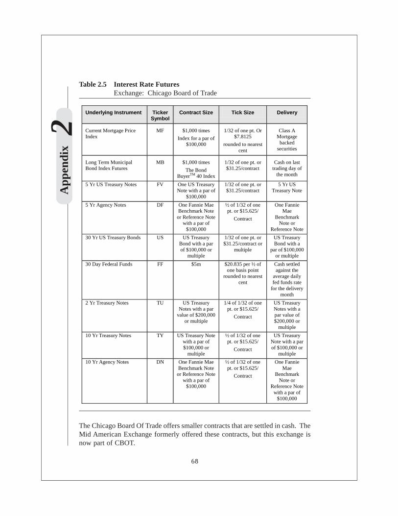
68
App
endi
x 2
Underlying Instrument
Ticker
Symbol
Contract Size
Tick Size
Delivery
Current Mortgage Price Index
MF
$1,000 times
Index for a par of $100,000
1/32 of one pt. Or
$7.8125
rounded to nearest cent
Class A
Mortgage backed
securities
Long Term Municipal Bond Index Futures
MB
$1,000 times
The Bond BuyerTM 40 Index
1/32 of one pt. or $31.25/contract
Cash on last
trading day of the month
5 Yr US Treasury Notes FV One US Treasury Note with a par of
$100,000
1/32 of one pt. or $31.25/contract
5 Yr US Treasury Note
5 Yr Agency Notes DF One Fannie Mae Benchmark Note
or Reference Note with a par of
$100,000
½ of 1/32 of one pt. or $15.625/
Contract
One Fannie Mae
Benchmark Note or
Reference Note
30 Yr US Treasury Bonds US US Treasury Bond with a par of $100,000 or
multiple
1/32 of one pt. or $31.25/contract or
multiple
US Treasury Bond with a
par of $100,000 or multiple
30 Day Federal Funds FF $5m $20.835 per ½ of one basis point
rounded to nearest cent
Cash settled against the
average daily fed funds rate
for the delivery month
2 Yr Treasury Notes TU US Treasury Notes with a par
value of $200,000 or multiple
1/4 of 1/32 of one pt. or $15.625/
Contract
US Treasury Notes with a par value of $200,000 or
multiple
10 Yr Treasury Notes TY US Treasury Note with a par of $100,000 or
multiple
½ of 1/32 of one pt. or $15.625/
Contract
US Treasury Note with a par of $100,000 or
multiple
10 Yr Agency Notes DN One Fannie Mae Benchmark Note
or Reference Note with a par of
$100,000
½ of 1/32 of one pt. or $15.625/
Contract
One Fannie Mae
Benchmark Note or
Reference Note with a par of
$100,000
Table 2.5 Interest Rate FuturesExchange: Chicago Board of Trade
The Chicago Board Of Trade offers smaller contracts that are settled in cash. TheMid American Exchange formerly offered these contracts, but this exchange isnow part of CBOT.

69
Appendix
2 Underlying Instrument
Ticker
Symbol
Contract Size
Tick Size
Delivery
US Treasury Bonds
XB
$50,000 par value
1/32 of one pt. Or
$15.62 per contract
Cash
US Treasury Bills
XT
$500,000 par value
1/2 basis point or
$6.25/contract
Cash
Eurodollars UD $500,000 1 basis point or $12.50/contract
Cash
5 Yr Treasury Notes XV $50,000 par value 1/32 of one pt. or $7.81/contract
Cash
10 Yr Treasury Notes XN $50,000 par value ½ of 1/32 of one pt. or $15.625/
Contract
Cash
Table 2.6 Interest Rate FuturesExchange: Chicago Board of Trade - Mid Am

70
Exe
rcis
es 2
1. An estate pays an annuity certain (cash payable whether or not the annuitantsurvives) of $50,000 per annum for five years. Assume the payments aremade at the end of the period. From the sixth year until the tenth year, thisannual payment will double. Determine the present value of the estate assuming8% per annum compound.
2. Find the present value of $500 payable monthly for six months. The first ofthe six payments occurs five months from now. The compound interest rate is1.1% per month.
3. Find the effective rate p.a. if the nominal rate per annum compounded quarterlyis 12%.
4. 12% p.a. nominal compounded monthly is equivalent to what nominal ratep.a. compounded quarterly?
5. 8% p.a. nominal compounded half-yearly is equivalent to what nominal ratep.a. compounded monthly?
6. Consider a bond with maturity date March 1, 2009, coupon 7% p.a. (paidsemi-annually). The market yield increases from 7% to 8% on March 1, 2001.On a face value of $1m., what is the percentage change in price? Is thisinstrument as sensitive as a zero coupon bond of identical final maturity pricedon the same day as the rate moves from 7% to 8%?
7. Price the coupon bond of Question 6 on the March 2, 2001 at 8% market yield.Why is there a price difference? (This problem is more difficult as there is apartial coupon period).
8. Price a seven-year zero coupon bond with face value $1m at a market yield of8% p.a. Assume semi-annual compounding. Price the same bond at a marketyield of 7% p.a. and compare its sensitivity with that of the bonds of Question6.
9. Calculate Macaulay duration for the bonds in Question 8, first at a yield of7%, then at 8%.
10. Price a 180 day T-bill with face value $1m when the bank discount rate is 7%.

71
Exercises
211. Price a 180-day CD at a market yield of 7%. Why is the price different from
that of the T-Bill in problem 10?
12. Suppose that the table below lists prices of two Eurodollar time deposit contractsquoted on the Chicago Mercantile Exchange on June 12, 2001.
Futures Contract BID OFFER
SEP 01 ED 94.25 94.26
DEC 01 ED 94.16 94.17
The date is June 12, 2001. A corporate treasurer wishes to increase workingcapital $40 million by drawing down a bank loan based on six-month LIBORon September 14, 2001. What financial risk does the corporate treasury facenow, and how can this risk be hedged using Eurodollar futures? Describe thehedge stating how many of which contract(s), the transaction involved (buy orsell) and the likely dealing price.
13. On June 12, 2001 a corporate treasurer managing a liability portfolio consistingof 22 million of ten-year fixed rate debt is considering interest rate forecastsin the ten-year area of the yield curve.
To what risk is the portfolio exposed, and why? How could the treasurer coveragainst this exposure using future contracts? Select the most appropriatecontract from Table 2.3. Then describe the hedge stating which contract,approximately how many to use, and the transaction involved (buy or sell).Would such a hedge remove all interest rate risk for the debt portfolio?

��

����������������������� ��� �������������
��
Until now, the notion of time and the way it is embedded into interest rates havebeen treated in a simplistic fashion. You may have noticed that although we weredealing with the valuation of cash flows of perhaps quite long maturity structures,the near-term parts of those cash flows were valued in the same way as the long-term parts, using the same interest rate as a discount factor. You might havewondered whether this is a good assumption to make, and you’d be right to wonder.Although it will suffice for an initial approach – and a good deal of practicalvaluation is done this way– it is not theoretically the best way to proceed. So wemust take a closer look at this issue. Even if you never end up using the tools of thischapter, reading through it will reinforce your understanding of the concept of interestrates.
This serves to introduce the topics of this chapter: zero coupon rates, implied forwardrates, and the way that they re-assemble into the term structure of interest rates.The term structure is all about the dependence of the interest rate structure onforward, or maturity, time. The notion of time itself gets a bit tricky, so we might dowell to start with some clarifying remarks on what we mean by time in this context.

��������������������� ����������������
��
����������������� ����������
3. 1 Notation and definitions
Arbitrage A zero-risk, costless investment strategy that generates aprofit. A no-arbitrage pricing or equilibrium is where no suchopportunities exist.
Long A position that benefits from a price rise and loses from aprice fall. In portfolio terms, a positive holding.
Short A position that benefits from a price fall and loses from aprice rise. In portfolio terms, a negative holding.
Hedge An instrument or position taken to reduce the exposure ofthe portfolio to adverse changes in value. A perfect hedgereduces the exposure to zero, but typically also results inzero upside potential.
Unit-discount bond A hypothetical zero coupon bond with a notional $1 facevalue.
Zero coupon bond Debt instrument that has no coupons, but merely a promiseto pay the face value at maturity. The reward element derivesfrom the discount at which it sells, relative to its face value.
Zero coupon rate The yield to maturity of a zero coupon bond; varies withmaturity time.
RT
The yield to maturity or IRR on a zero coupon bond ofmaturity T.
f t
The implied forward rate is the implied one period interestrate for future period t priced into an instrument such as abond or swap by the market at current time.
Term structureof interest rates A graph of zero coupon rates, yields, or implied forward rates
against maturity time.
Yield curve The term structure curve applied to yields.
Spot rate The interest rate for the one period immediately ahead, knownas of the current date.

��
������� ��������������� ���� ����������������
Bootstrapping A sequential methodology using actual bond prices andcoupons to derive the zero coupon term structure.
3.2 A brief mystery of time
Suppose you are at time 0 (t = 0), the present time, and are looking at T-bill rates.You are concerned about them, because you know that your very expensiveadjustable-rate mortgage is partially tied to them.1 You might form an impressionof what the T- bill rate will be for every six-month period throughout the next tenyears, as though you had a mental image of the rate at six-month intervals fromnow (t = 0) until t = 20. For convenience, we have adopted the basic time intervalof six months.
The notion of time for this mortgage planning scenario is both a current as well asa forward concept. The expression forward time (and forward rate in the nextparagraph) is adopted to distinguish it from the current time (and the current rate,which will be known as the spot rate). Thus, forward time (i.e. t >0) must alwayshave the current time as a base. Here, forward time is the 20 six-month periodsfollowing current time, t = 0. Current time is in real time, while forward timerefers to the future. Real time refers to the actual passage of time.
Suppose that at real time t = 0, the T-bill rate over the coming six-month period is i1
(the periodic rate used in Chapters 1 and 2). You could also form an estimate of thenext six-month T-bill rate, which is known as the forward interest rate f
1. It has to
be a forward rate, because you won’t know the true six-month T-bill rate at time1 until six months has passed.
Figure 3.1 illustrates this concept. The eye represents you looking forward into thefuture. At any point in actual or real time (denoted t), you will know what thecurrent one period rate is, because this is set by the market now to apply over thecoming unit period (here we use six months). At real time t = 0 you know i
1, at real
time t = 1 you know i2, and so forth.
But at time t = 0, you don’t know what i2 will be. Only when real time has moved
forward to t = 1 will you know, so in the meantime, you have to form an estimate ofi2. This is denoted as f
1. Now imagine you are six months older and can see what
the actual six-months rate is in real time t = 1. The new spot rate (i2) will almost
certainly differ from your guess at t = 0 about the forward rate, f1. In other words,
generally speaking, i2 ≠ f
1.

��������������������� ����������������
��
����������������� ����������
Figure 3.1 Real versus forward time
������� �� �� �� ��
������� �� ��
������� �� ��
���
����
����
��������
�������
���� ���
���������� ���� ������ �����
���������� ���� ������ ����
���������� ���� ������ �����
In the following discussion, we shall call the i rates the spot rates. They are theactual one-period rates observed in real time. Hence, i
t means the actual one-
period rate that applies for period t, measured at the instant in real time t - 1. Byperiod t, we mean the time period which begins at the instant in real time, t -1, andruns to real time, t. Period 1, therefore, runs from the instant real time t = 0 to theinstant real time t = 1.
We shall also assume general units of time, which may correspond to a year, a six-month period, or whatever time unit applies. By using t as the time unit, we assumethat this is the basic discounting or rest period, so that interest rates are measuredusing the same unit of time. For example, if the annual rate is 4 % for six-month T-bills, and if t refers to six-month intervals, then the spot interest rate is 2%.
3.3 Zero coupon rates
A current one-period unit discount bond would be an instrument that pays back $1at future time 1 (t = 1). It is the simplest example of a zero coupon bond, one forwhich the face value is just one dollar. Suppose that the market prices this bond atP
1. Its yield, R
1, is then given by:
1 Lenders base ARM rates on a variety of indexes. Among the most common are the rates on one-, three-, or five-year Treasurysecurities. Another common index is the national or regional average cost of funds to savings and loan associations. A fewlenders use their own cost of funds, over which – unlike other indexes – they have some control. As a borrower, you shouldfind out which index will be used, how often it changes, how it has behaved in the past, and where it is published.
��
������� ��������������� ���� ����������������
R +
= P1
11
1, thus R1 =
1
1
P-1.
Note that the subscript 1 indicates that this is a one-period instrument, as seen fromreal time t = 0. The one-period zero coupon rate is also the IRR – the interest ratethat equates the price to present value of the $1 terminal cash flow. Since this is aone-period instrument, the IRR is also a one-period rate.
Suppose that at t = 0, we have available a two-period pure discount bond.Technically, this is now a zero coupon instrument because there is no coupon paidat time 1. Its price and yield have an inverse relationship, following Equation (8)from Chapter 1, so that:
R +
= P 22
2)1(
1 ; thus R2 = 5.0
2
1
P
-1.
Will R2 be the same as the one-period rate R
1? Not necessarily. After all, with the
two-period instrument we are tying our money up for two periods—we might expectsome extra compensation since this reduces our liquidity.
We can continue this example for three time periods, four time periods, and so on,solving for the various yields. In general:
( )1
1;
1
11
−
=
+=
t
ttt
t
t PRthus
RP (1)
All the interest rates we have derived – the zero coupon rates – are computed at t= 0. Consequently, everything is seen from the same point in real time – thepresent. The plot between R
t (zero coupon rates) and t, with t on the horizontal
axis (maturity), is called the zero coupon rate term structure of interest rates.Note that by convention, all rates are annualized in the graph.
Figure 3.2 illustrates a zero coupon rate term structure. This particular version hasthe rate increasing with maturity; it is upwardly sloping. An upward sloping termstructure is known as a normal yield curve. Most theories on term structure suggestan upward slope, and this is often what we see in the “real” world. The opposite—a downward sloping curve—where the shorter rates are higher than the longerrates, is known as an inverted yield curve. This would not be considered a normalstate of affairs; it is characteristic of periods of tight monetary control. Humpedcurves also surface from time to time, and some evidence suggests they presage arecession.

��������������������� ����������������
�
����������������� ����������
5.4
5.6
5.8
6
6.2
6.4
6.6
6.8
0.00 2.00 4.00 6.00 8.00
forward time (years)
zero
co
up
on
rat
e %
Figure 3.2: Zero coupon term structure
If we knew the zero coupon rate structure—in other words, the entire sequence(R
1, R
2, R
3...R
T)—we could use this data to value any set of cash flows into the
future. An obvious example is a coupon bond of maturity T periods and face valueFV. Its zero coupon based valuation would be:
PT
= R +
FV + C + . . . +
R +
C +
R +
CT
T )1(
)(
)1(1 221
(2)
If market participants evaluate coupon bonds this way, what does this indicate? Itsuggests simply that each coupon can be viewed as the payoff of a zero couponbond. For instance, the second term on the right hand side of Equation (2) is thevaluation of a zero coupon bond of face value C, received at the end of period 2.This analogy is true for all of the cash flows, including the last (T-period) payment,which is (C + FV). Doing this effectively strips the coupons from a standardcoupon-bearing instrument, creating a series of zero coupon bonds. The USgovernment does not issue zero coupon bonds. However, investment companiesnoticed in the early 80’s that there was large potential demand for “stripped”treasuries. In 1982, Merrill Lynch and Salomon Bros. created the first widelytraded synthetic treasury zeros. These securities are still popular.
Would the price in Equation (2) be the same as the evaluation based on yields asper Equation (9) in Chapter 2? Theoretically, yes. The yield (i) used in Chapter 2

�!
������� ��������������� ���� ����������������
turns out to be a weighted average of the T zero-coupon yields. If the bond marketis characterized by many actively traded bonds of differing maturities so that asufficientset of zero coupon rates can be backed out, then the two equations should generatethe same result. In well-developed bond markets (like those in the US), arbitrageursstand ready to buy and sell different baskets of bills, notes and bonds looking for anarbitrage profit. This activity quickly erases any pricing differences in the twoequations. However, in smaller bond markets around the world we see incompletebond maturity sets and/or trading liquidity problems, which may impede the arbitrageprocess.
3.4 Implied forward rates
Recall that RT refers to the equivalent one-period interest rate which would apply
over the entire maturity of a particular zero coupon bond. For example, R2 refers
to an average one-period rate applied over two periods. Can we break R2 down
into constituent parts, one for each of the two periods that make up the two-perioddiscount calculation? The answer is yes, as we shall see.
Reconsidering Figure 3.1, imagine we are at time t = 0 and wish to invest $1 for justone period. You can see that the one-period zero coupon rate R
1 and the spot rate
(i1 or f
0) are the same. Your dollar would accumulate to:
1 + R1 = 1 + f
0
dollars at the end of period 1.
However, imagine that at t = 0 you had wanted to commit your funds for twoperiods. There are now two ways of writing the resulting accumulated value, andboth must be equal:
(1 + R2) 2 = (1 + f0 )
× (1 + f1 )
The left hand side of this equation says that because you are tying up your moneyfor two periods, you must earn the two-period yield R
2. The right hand side suggests
that this can also be regarded as two one-period investments, one after the other.You invest at rate f
0 (= i
1) over the first period. Then you invest the proceeds (1 +
f0 ) over the second period at rate f
1 to get (1+ f0)× (1 + f1 ).
Since f0 = R
1, we can back out what the f
1 must be by solving the above equation
to get:

��������������������� ����������������
"
����������������� ����������
f1 = 1
)1(
)1(
1
22 −
++
R
R (3)
The whole process can be extended to time periods further into the future, torecover all the implied forward rates in terms of the zero coupon rates.
In general, if we have the zero coupon rates for time t + 1 and for time t, we cancalculate the forward rate t periods from now. The implied forward rate, f
t, for
maturity t in the future is given implicitly by:
(1 + Rt+1) t+1 = (1 + Rt )
t × (1 + ft )
or explicitly by:
ft = 1
)1(
)1( 11 −
++ +
+t
t
tt
R
R (3�)
Hence, if you have a series of zero coupon rates (R1, R
2, R
3 . . .), you can always
back out a corresponding series f0, f
1, f
2 of implied forward rates.
There is an approximate averaging relationship between the zero coupon rates andthe implied forwards:
( ) . f + ... + f + f t
R tt 110
1−×≈ (4)
The wavy equal sign means “approximately equal to.” The approximation becomesexact as the compounding interval gets smaller and smaller. At any rate, you canthink of the R’s as the average of the f’s. An exact (rather than approximate)relationship says that (1+R
t)t = (1 + f
0 ) (1 + f
1 )…(1 + f
t-1 ). If you are mathematically
inclined, you will know this means that the t-period zero coupon accumulation factoris the geometric average of the one-period accumulation factors 1 + f
0, 1 + f
1, …(1
+ ft-1
).
The term structure can also be portrayed in terms of the f’s, that is, by plotting fagainst forward time t. This is called a forward rate term structure. In manyways, it is better than the term structure based on the zeros, as it gives you themarket’s estimates of the future spot rates at the particular time interval. In business,many think that marginal rates are always more useful than average rates, whetheryou are looking at interest rates or tax rates.

#
������� ��������������� ���� ����������������
Figure 3.3. Implied forward versus zero coupon term structure
Figure 3.3 plots a forward rate term structure and the corresponding zero couponterm structure (the curve with a hump) on the same diagram. The averagingrelationship referred to earlier means that the graph for R tends to follow that for f.This is why the peak in R occurs after the peak in f.
3.5 Forwards, futures and no-arbitrage
Are forward rates and forward prices related? The following discussion will showus that they are. But before discussing this relationship, we need to review someof the concepts from Chapter 2.
Recall that forward contracts are an agreement calling for future delivery of anasset at a price agreed upon at the inception of the contract. A futures contract isa forward contract that is exchange traded and marked to market, i.e. valued everyday. To assist tradability, the futures contract is standardized for units, quality andquantity. As the following example will show, forward rates bear some relationshipto forward or futures prices on these instruments.
Recall also the definition of hedging—investing in an asset to reduce risk. Theconcept of a perfect hedge is integral to the discussion that follows. If you are longan asset, the hedge would be to short a futures (forward) contract. If you were
5.2
5.4
5.6
5.8
6
6.2
6.4
6.6
0.00 2.00 4.00 6.00 8.00
forward time
forw
ard
rat
esze
ro c
ou
po
n r
ates
zero coupon
forward rate
��������������������� ����������������
�
����������������� ����������
short the asset, the hedge would be to go long on a futures (forward) contract onthe asset. If a hedge is perfect, you reduce the price risk of the portfolio to zero.
For the purposes of this example we will discuss contracts on unit discount bondsand ignore the trading complexities of the various interest rate contracts discussed in Chapter 2. By doing this, we ignore the peculiarities of each of these contractswhile pointing out the relationship between forward (futures) prices and forwardrates.
Imagine a simple two-period scenario. Period one spans the interval between t =0 and t =1, while period two spans the interval from t = 1 to t = 2. Let’s supposethat today (t = 0) you enter into a contract to deliver a one-period unit discount bondone period from now (that is, t = 1) for an agreed upon price, F. In other words,after the passage of one period of time, you will deliver to the other person in thecontract a one-period unit bond, and the other person will give you F in exchange.The next topic of our discussion is the no-arbitrage price F, which is the price tobe quoted in the market now so that nobody can make money for certain whenseen as of time 0, the current time.
First, some notation:
F = price of a one period bond agreed at t = 0 for delivery at t = 1
=1P price of a one period unit discount bond at t = 0
=1
~P price of a one-period unit discount bond at t = 1
=2P price of a two-period unit discount bond at t = 0
Note the distinction between P1 and 1P
~. The first refers to the price of the one-
period bond at the current time (t = 0). The second refers to the price of the one-period bond at t = 1. The tilde symbol over the P in 1P
~indicates that it is a random
variable (one whose outcome is yet unknown). Indeed, 1P~
is unknown at time t =0.
Now back to the problem of determining F. You have sold a one-period bondforward, so now you have an exposure to 1P
~, the price of the one-period bond
you will have to use to deliver on your forward commitment. One characteristic ofarbitrage is that your position be risk-free, so that at inception, you have to cover

�
������� ��������������� ���� ����������������
� �
�������� �������
�������
��
���
��
��
���
�
�
The following table lists the contents of this timeline and shows the detail of thecash flows at t = 0 and at t = 1.
�����������������
����������
�� ���������������������������������������������������������������������������������������
!�
"��#�!�
"��#�!�� �!�
���
� ��
"�
�
���� �����
�
the above end-of-period exposure to 1P~
. Another characteristic is that trueprofessional arbitrage plays should cost no money of your own. So how do wemanufacture this?
First, we have to cover the exposure described above. To do so, go long (that is,buy) a two-period discount bond now. At the end of the period, it will have become
a one-period discount bond. Being long in this bond will cancel exposure to 1P~
.
Of course, going long will cost money, as we have to purchase the two-periodbond. To fund this purchase, we will borrow against the cash flow of $F to bereceived at time t = 1. This one-period borrowing is done via the issue of F one-period unit bonds at price P
1 . (Note that P
1 is the known price at t = 0 of a one-
period bond). Thus, we borrow $(F × P1 ) which is noted as a cash inflow (+) while
the purchase of the two-period unit bond is noted as a cash outflow (–). Let's drawa timeline to illustrate these transactions.

��������������������� ����������������
�
����������������� ����������
Because of the way this example is constructed, the actions in the present (t = 0)result in a net zero cash flow in the future (t = 1). What should a portfolio that isworth $0 in the future be worth today? The answer must be zero. We can takethis result and set the total cash flow at t = 0 to $0, or F×P1-P2= 0. Rearranging theterms, we get:
F = P
P
1
2=
bond period one of price
bond period two of price (5)
We know from Equation (1) that:
P1 = )1(
1
1R+ , and
P2 = 2
2 )1(
1
R+ ,
so,
P
P
1
2= 2
2
1
)1(
1
R
R
++
.
Equation (3) allows us to back out the one-period forward rate one period fromnow. This, along with the equation above, tell us that the forward or futures price,F, is equal to:
F = 11
1
f+ (6)
This is why f1 is called the implied forward rate. It represents a market certainty
equivalent discount rate formed at t = 0, to enable it to price now a one-perioddiscount bond for delivery at instant t =1, which is future time. More generally, theforward rates f
0, f
1, f
2, etc., represent a pricing device by which the forward
component of any current price can be calculated.
Returning to the example above, let’s insert some actual numbers.

�
������� ��������������� ���� ����������������
R1 = 2.5%; P
1= $.9756098
R2 = 3.0%; P
2= $.9425959
F= .9661608
The two cash transactions at t = 0 are to buy a two-period discount bond now at$.9425959, and issue F one-period unit bonds at $.9756098. Thus, we have borrowed$(F × $.9756098) and this is noted as a cash inflow (+), while the purchase of thetwo-period unit bond is noted as a cash outflow (-). The value of F we havecalculated as 0.9661608, while that of 1
~P is still unknown, so we simply use a
symbol. We will redraw the timeline to incorporate these cash flows.
� �
�������� �������
���#����������
���������
���
���
����������
����������
�
�
�����������������
����������
�� ��������������������������������������������������������������������������������������
$%&��'&'&
���#� $%&(')&*
���#�$%&(')&*� �$%&��'&'&
���
� ��
��
�
���� �����
�
The no arbitrage condition tells us that F× $.9756098 -$.9425959 = 0. Rearrangingterms we see that:

��������������������� ����������������
�
����������������� ����������
F = P
P
1
2=
$.9756098
$.9425959= .9661608
Using Equation (6) and F = .9661608, we find that f1 is 3.50244%. Of course, our
current purpose is illustrative, and we do not need to go through all these calculationsin order to obtain the implied forward rates! To find the rates, simply use Equation(3) or (3r) above.
3.6 Computing zeros and forwards
The correct way to compute the zero rates is from an actual series of zeros or frombonds that have been stripped and repackaged as zeros. To estimate the entireyield curve and forward rates we would need an entire series of such bonds. Whatif there are not enough zeros or strips? This is not a problem if you have prices ona set of coupon bonds that span the maturity horizon for the yield curve (as in theUS—there are over 150 government bonds listed in the Wall Street Journal withmaturities ranging from one day to 30 years). At any rate, suppose you have threecoupon bonds with coupons C
1, C
2, C
3 and maturities one, two and three periods.
The market quotes them at prices P1, P
2, P
3, respectively. In terms of the zeros,
the bond prices can be decomposed and written (with subscripts denoting the bond):
;1 1
11 R
FVCP
++=
;)1(1 2
2
2
1
22 R
FVC
R
CP
+++
+=
.)1()1(1 3
3
32
2
3
1
33 R
FVC
R
C
R
CP
+++
++
+=
Notice how the bonds are valued. As observed in Section 3.3, we are decomposingthem into their constituent cash flows. A coupon received at time three is itself justlike a zero coupon bond of face value C
3 maturing at time three.
Once the market quotes the three prices, you can solve for the three zero couponrates implied by those prices. Just solve the three simultaneous equations above.Of course, once you have the zeros, getting the implied forwards is straightforward.
Instead of using prices, market yields are often used to back out zeros. We haveused yields – or internal rates of return – very extensively in Chapter 2. Up to this

�
������� ��������������� ���� ����������������
point, however, we have not mentioned the relationship between these yields andthe zeros or implied forwards, so we need a digression on this.
Yields, zeros and swaps
You can also do a term structure based on yields. Suppose you had threecoupon bonds, as above, being quoted at market prices P
1, P
2, and P
3. You know
the yields on these bonds will all be different. We will use the symbol ρ for theyield, as it is often used for the internal rate of return, and the yield is just anIRR. So the three yields ρ
1, ρ
2, ρ
3 are defined implicitly by the equations (the
subscripts denote the particular bond):
;1 1
11 ρ+
+= FVCP
;)1(1 2
2
2
2
22 ρ+
++ρ+
= FVCCP
.)1()1(1 3
3
32
3
3
3
33 ρ+
++ρ+
+ρ+
= FVCCCP
In other words, once you know the prices, you can recover the three yields tomaturity, namely ρ
1, ρ
2, and ρ
3, for the different maturities. You can also plot
these yields against time, which would give you a yield-based term structure—yet another version of the term structure.
We have seen that one can switch readily between zeros and implied forwards –they are simply different aspects of the same thing. Can you also do the same asbetween yields and zeros? The answer is “yes and no.” It depends upon whetheryour coupon bonds, as in the example above, are trading at par. You will recall thata bond trades at par if the current price, P, is equal to the face value, FV. It turnsout that if the bonds are not trading at par, then there is no simple relationshipbetween the yields and the zeros.
Indeed, the yield to maturity depends on the coupon to face value ratio(the couponyield), so the maturity alone is not sufficient information to determine the yield.The yield depends on various characteristics of the particular bond. This makesmatters a bit inconvenient. If you have two three-year bonds with different coupons,they will have quite different zero coupon-based prices, and possibly different yieldsas well. There is no simple relationship, independent of the coupon, between yieldsand zeros. In fact, if you do price different three-year bonds using the same the

��������������������� ����������������
����������������� ����������
three-year yield computed off just one of them, you could face arbitrage by someonewho has calculated the price correctly using zeros. Recall that zeros are independentof coupons, face values, etc., and are the same for every bond. In this sense, thezeros—not the yields to maturity—would be the correct way to price the bond.
If you calculated the yield to maturity on a bond that happened to be trading at par,you could in fact recover the zeros. One example where trading at par for a fixedinterest instrument always occurs is with an interest rate swap, just placed on thebooks. An interest rate swap is an agreement between two parties, whereby eachcontracts to make interest payments to the other on specific dates in the future.
The standard interest rate swap involves an exchange of fixed rate payments,which we will refer to as coupons, determined at the inception of the swap, for aset of floating rate payments determined on specified rate setting dates. Both fixedand floating payments are calculated on a notional principal amount that neverchanges hands. These floating rate payments are typically based on the six-monthLIBOR rate (the rate for six-month interbank dollar deposits set in London) oneach rate set date. In fact, swaps can come in all sorts of flavors, but this is a basicor “plain vanilla” swap.
A swap has a zero value when placed on the books. It represents a free exchangeof one sort of payment for another. The fixed side (at inception) is valued asthough it were a coupon bond selling at par. The floating side represents marketindifference between such a coupon bond and the series of future floating ratepayments. So here it is: the yield on the fixed side of the swap at its inceptioncan be taken as a par yield.
Swaps are quoted in standard maturities of one, two, three, four, five, seven and tenyears, with in-between maturities usually calculated by applying a linear interpolation.For example, a six-year swap would typically be quoted with a fixed rate half waybetween the five- and seven-year par yields. Using the yield to maturity of themany different swap maturities, you can calculate backwards to find the zero couponrates. In the next section, we give you an algorithm, suitable for use in a spreadsheet,to do just this.
!
������� ��������������� ���� ����������������
3.7 Algorithm: computing zeros and forwards from swap data
“Plain vanilla” (or standard) swaps are quoted on the basis of a constantly changingcoupon and equivalent yield, so they are traded at par when transacted. They are,however, an over-the-counter product, and even swaps quoted on the same dayand same maturity are not usually homogeneous. As market prices of bonds, futures,and so on move from one minute to the next, so does the swap rate (which representsboth the coupon and the yield). As we’ve discussed, you cannot expect that a setof cash flows with the same maturity but different coupons can be correctly pricedat the same yield. Sometimes this will turn out to be the case, but more often it willnot. Hence, it is impossible to value one-day-old (even one-minute-old) swapsusing yields to maturity.
Swaps are always valued by applying the current swap zero-coupon curve. At theoutset, the zero-coupon valuation gives the same answer as a valuation using theyield, but not after time ticks onward and swap rates move. At any given point intime, new swaps are quoted on a yield basis, often as a spread over a governmentbond yield curve, and the current swap zero curve can be obtained from the swap“yields” by the following iterative process.
Backing out the swap zeros
Suppose that we find that the US swap market is currently quoting the followingswap rates, displayed in Table 3.1, on a percentage per annum basis. We have justlisted mid-rates out to three years to simplify matters. (The full range can go outten years or more for top credit counterparties.) The following algorithm alsoabstracts from the complexities of day-count conventions by using a semi-annualcoupon, equal to half the annual coupon rate times the notional principal (bondbasis). The semi-annual yields are just the current par swap rates divided by two.
In the US market, swaps are frequently quoted with an annual Actual/360 coupon,with the floating leg based on six month LIBOR, paid semi-annually. Our simplifiedexample illustrates the methodology for calculating the zero-rates without gettingbogged down in day-count issues. It can readily be adjusted to handle any of thevarious day-count conventions used in the different swap markets.

��������������������� ����������������
!"
����������������� ����������
Table 3.1 Par swap rates
Maturity (years)
Period
(t)
Par Swap Rate
(% p.a.)
0.5
1.0
9.53 (LIBOR rate)
1
2.0
9.08
1.5
3.0
8.84
2
4.0
8.6
2.5
5.0
8.5
3
6.0
8.4
Step 1 The first point on the zero curve is the easiest. It is simply the six-monthbank bill rate which is itself a zero coupon rate. The first discount factord
1 is therefore:
.95451725.0
20053.9
1
11 =
+=d
Step 2 If we take the fixed side of a current one-year semi-annual swap withface value of 100, and use the discount factor d
1 to value its first cash
flow, we can solve for the second zero rate. It must be the rate whichvalues the second cash flow at an amount that will bring the total valueof the fixed cash flows (including the final flow of principal) back topar—i.e., equal to 100.
That is:
Here C1 is the “coupon’” for a current one-year swap, which per hundred face
value on a swap paying on a semi-annual basis is:
. R +
+ C + +
C =
2001
100
200
53.91
1002
211

!#
������� ��������������� ���� ����������������
Calculating the right side of the equation, we obtain:
. = R +
= d
2
91511854.0
2001
1
22
This is our second discount factor.
The discount factor is very useful as it stands for discounting one-year cash flows,but we will take the next step and solve for R
2 as well:
. = - = R 069808.9200191511854.
15.02 ×
Step 3 As the 1.5 year swap rate is 8.84% p.a., the semi-annual coupon will be:
42.42
84.85.1 ==C
.54.42
08.91 ==C
We can plug the value for C1 into (8) as follows:
,
2001
10054.4
20053.9
1
54.4100
22
+
+++
=R
and then rearrange to get:
. .
+
= R +
54104
1
200
53.91
54.4100
2001
1
22
×
−
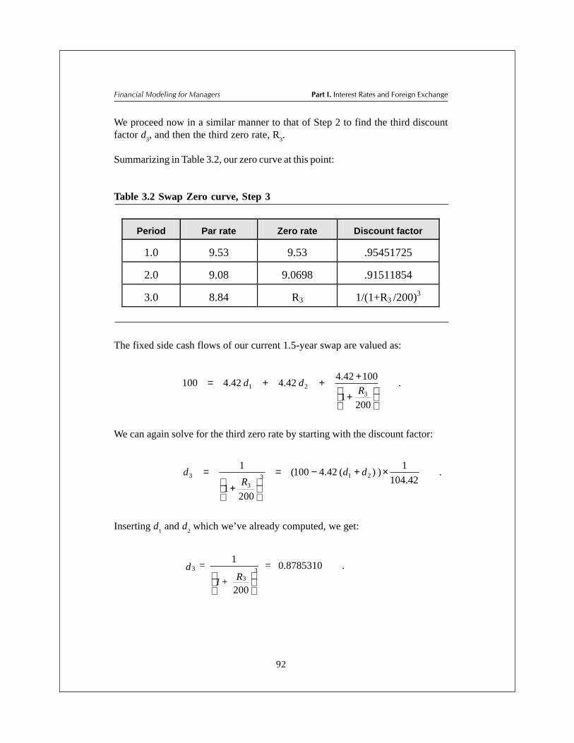
��������������������� ����������������
!�
����������������� ����������
We proceed now in a similar manner to that of Step 2 to find the third discountfactor d
3, and then the third zero rate, R
3.
Summarizing in Table 3.2, our zero curve at this point:
Table 3.2 Swap Zero curve, Step 3
The fixed side cash flows of our current 1.5-year swap are valued as:
.
2001
10042.442.442.4100
321
+
+++=R
dd
We can again solve for the third zero rate by starting with the discount factor:
.42.104
1))(42.4100(
2001
1213
3
3 ×+−=
+
= ddR
d
Inserting d1 and d
2 which we’ve already computed, we get:
.8785310.0
200
1
333 =
R + 1
= d
Period
Par rate
Zero rate
Discount factor
1.0
9.53
9.53
.95451725
2.0
9.08
9.0698
.91511854
3.0
8.84
R3
1/(1+R3 /200)3

!�
������� ��������������� ���� ����������������
Table 3.3 Swap Zero curve, Step 4
Period
Par rate
Zero rate
Discount factor
1.0
9.53
9.53
.95451725
2.0
9.08
9.0698
.91511854
3.0
8.84
8.82266
.8785310
4.0
8.60
R4
1/(1+R4 /200)4
In turn, we obtain:
.8226618.820018785310.
13333.03 = = R ×
−
Step 4 Next, find the fourth discount factor and zero rate, using the threepreceding discount factors and applying the same process as above. Thetwo-year (fourth period) swap rate is 8.60% p.a., giving a coupon rateof:
.30.42
60.80.2 ==C
We can express the value for the fixed cash flows of a current two-year swap as:
,
2001
10030.430.430.430.4100 4
4
321
+
++++=R
ddd
and find the two-year (fourth period) discount factor:
.8454735.30.104
1))(30.4100(
2001
13214
4
4 =++−=
+
= dddR
d

��������������������� ����������������
!�
����������������� ����������
and then find the fourth zero rate:
.571517.820018454735.
125.04 =×
−=R
You can see how it goes: you arrive at the discount factors d1, d
2, d
3. . . recursively
from the previous ones. Once you have each dt, you can easily obtain the associated
zero curve rate Rt. Now you can test your understanding of these concepts by
recovering the remaining dt and R
t for the data of Table 3.1. You should be able to
calculate the discount factors and zero rates as shown in Table 3.4.
Table 3.4 Swap Zero curve to three years
Period (t)
Par rate
Zero rate Rt %
Discount factor
1.0
9.53
9.53%
.95451725
2.0
9.08
9.06981
.91511854
3.0
8.84
8.82266
.87853103
4.0
8.60
8.57152
.84547347
5.0
8.50
8.46868
.81272929
6.0
8.40
8.36320
.78208491
Finding the forward rates
For the last part of this example, we will calculate the one-period forward curve,f0, f
1, . . . f
n from the zero rates above.
Retrieving Equation (3) from Section 3.4 and modifying it slightly to adjust for oursemi-annual data, we can apply it to the zero rates we have calculated.

!�
������� ��������������� ���� ����������������
.1)1(
)1(
1
22
1 −+
+=R
Rf (7)
Recall that the first forward rate, f0, is simply the zero rate, R
1, which is 9.53% on
Table 3.4. The next forward rate, f1 is found by plugging R
1 and R
2 from the same
table into Equation (7a) as follows.
.21
21
21
1
22
1 R
R
f ×
−+
+
=(7a)
.%6106.8..0861063.021
2093.0
1
2090698.0
12
1 eif =×
−+
+
=
To find the remaining one-period forward rates, we need a more general form of(7a), which we will call (7b):
.21
21
21
11
1R
R
ft
t
tt
t ×
−
+
+
= −−
−(7b)
The third forward rate is then:
.%..
.
.
32928 i.e.,083292021
20906980
1
208822660
1f
2
3
2 =×
−
+
+
=

��������������������� ����������������
!�
����������������� ����������
The fourth forward rate, f3 is:
.%8199.7..078199.021
20882266.0
1
2085715.0
1
3
4
3 eif =×
−
+
+
=
The one-period swap forward rates and zeros derived from the original (threeyear) swap par curve of Table 3.1 are collected in Table 3.5 below. You can testyour understanding of this section by attempting to produce the fifth- and sixth-period rates yourself. Better yet, produce the curves out to five years using theaugmented data given in Table 3.6 in the exercises at the end of this chapter. Sucha set of calculations is most easily performed using a spreadsheet program such asExcel or Lotus. If you are not familiar with these programs, particularly withrespect to financial calculations, you may find it helpful to skip ahead to Chapter 5,which provides an introduction to spreadsheets.
Table 3.5 Swap Zero and Forward curve to three years
Period (t)
Par rate %
Zero rate Rt %
Forward rate ft-1 %
1.0
9.53
9.53%
9.53%
2.0
9.08
9.06981
8.61063
3.0
8.84
8.82266
8.32925
4.0
8.60
8.57152
7.81989
5.0
8.50
8.46868
8.05783
6.0
8.40
8.36320
7.83659

!�
������� ��������������� ���� ����������������
3.8 Concluding remarks
Modern fixed-interest pricing theory operates using zeros, and especially, impliedforward rates. A popular approach to modeling the term structure is by assumingthat there are only a few primary drivers in determining forward rates. Thesefactors are assumed to drive not only the forward rates, but flow through these tothe entire term structure and the pricing of fixed interest products.
Although we have presented our discussion in terms of discrete time, these conceptsare more naturally cast in terms of continuous time discounting. This notion wasintroduced in Section 2.5, but there the term structure was effectively assumed tobe flat, so there was only one interest rate to worry about. Where there areseveral forward rates, the representative discount factor – equivalent to the priceof bond of continuous maturity T – is given by:
. e dt f = P t
T
0
- T ∫
In this equation, the discounting process occurs over a sequence of small intervalsfrom t to t + dt, and at each interval, the instantaneous forward rate f
t is applied in
forward time t. The zero coupon rate for the interval (0,T) is defined by:
. dt f T
= R t
T
0
T ∫
1
Bearing in mind that the integral is just a sum, you can see that the zero rate is justthe arithmetic mean of the instantaneous forward rates. We could also write thediscounting formula as:
, e = P R T - T
T
and the relevance to the discussion of continuous discounting in Chapter 2, Section5, should be clear.

!
We have not discussed the topic of the term structure in much detail, nor explainedwhat determines the way the term structure curve shifts through time(as it hascertainly done recently in many countries). There are several theories about theterm structure. One long-standing theory is that the forward rates can be regardedas expectations of future spot rates, conditional on information available at timezero. For instance, if you expect that two years from now, the Federal Reservewill be adopting a tighter monetary stance which would affect short-term interestrates, so you are expecting the spot rate in two years time to be high. Under thepure expectations theory, you revise your current forward rate upwards for twoyears out. The theory is sometimes augmented to include risk influences, whichgenerally increase with forward time, since future events are viewed as beingmore risky.
We have not yet finished with the topic of interest rates, which will become importantas we go on to discuss foreign exchange. However, what has been covered so farwill serve as an introduction to this huge and multi-faceted topic, which is of immenseimportance in financial management.

!!
Exercises
3The basic data needed for the following questions is contained in the table below,an augmented version of Table 3.1 which appeared earlier in the chapter.
Table 3.6 Par swap rates
Maturity (years)
Par Swap Rate
(% p.a.)
0.5 9.53 (6-month LIBOR rate )
1.0
9.08
1.5
8.84
2.0
8.60
2.5
8.50
3.0
8.40
3.5
8.35
4.0
8.30
4.5
8.27
5.0
8.24
1. Use the swap zero coupon rates to value two coupon bonds, each with facevalue $1,000,000 with maturity five years but with differing six-month couponrates as follows:
(i) A coupon rate of 10%(ii) A coupon rate of 5%
(Begin by computing the zero rates for the last four time periods.)
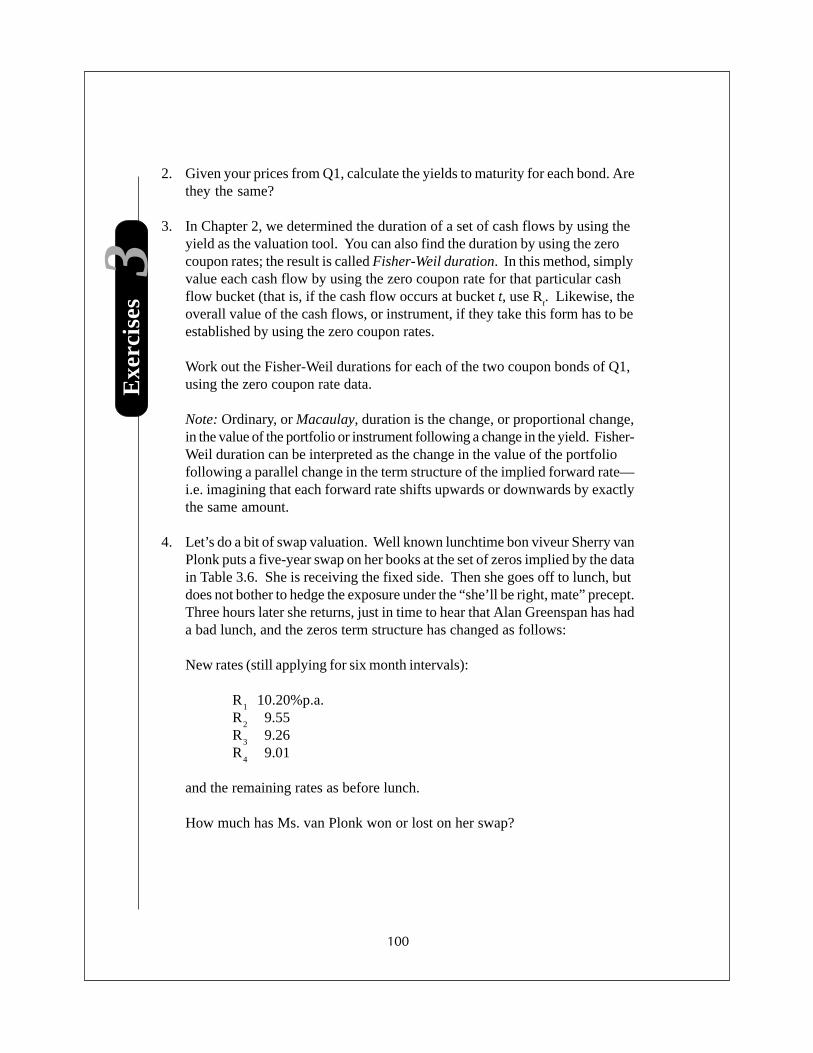
#""
Exe
rcis
es 3
2. Given your prices from Q1, calculate the yields to maturity for each bond. Arethey the same?
3. In Chapter 2, we determined the duration of a set of cash flows by using theyield as the valuation tool. You can also find the duration by using the zerocoupon rates; the result is called Fisher-Weil duration. In this method, simplyvalue each cash flow by using the zero coupon rate for that particular cashflow bucket (that is, if the cash flow occurs at bucket t, use R
t. Likewise, the
overall value of the cash flows, or instrument, if they take this form has to beestablished by using the zero coupon rates.
Work out the Fisher-Weil durations for each of the two coupon bonds of Q1,using the zero coupon rate data.
Note: Ordinary, or Macaulay, duration is the change, or proportional change,in the value of the portfolio or instrument following a change in the yield. Fisher-Weil duration can be interpreted as the change in the value of the portfoliofollowing a parallel change in the term structure of the implied forward rate—i.e. imagining that each forward rate shifts upwards or downwards by exactlythe same amount.
4. Let’s do a bit of swap valuation. Well known lunchtime bon viveur Sherry vanPlonk puts a five-year swap on her books at the set of zeros implied by the datain Table 3.6. She is receiving the fixed side. Then she goes off to lunch, butdoes not bother to hedge the exposure under the “she’ll be right, mate” precept.Three hours later she returns, just in time to hear that Alan Greenspan has hada bad lunch, and the zeros term structure has changed as follows:
New rates (still applying for six month intervals):
R1
10.20%p.a.R
2 9.55
R3
9.26R
4 9.01
and the remaining rates as before lunch.
How much has Ms. van Plonk won or lost on her swap?

#"#
Exercises
35. During their very enjoyable lunch, well known tax consultant Darth Evader has
suggested to Ms. van Plonk that she do him a swap whereby he will make asingle payment up front, in return for a set of floating payments out to fiveyears. The nominal or face value of the swap will be $1m.
(i) Using zeros for the valuation, what should Ms van Plonk be asking him topay?
Assume pre-lunch interest rates and ignore commission and othertransaction costs.
(ii) Would such a swap be more or less exposed to the post-lunch change ininterest rates?
6. Find the Fisher-Weil duration of the swap in Question 4 above (valued usingthe post-lunch rates).

102
FourFourFourFourFourFX Spot and Forwards
103
Around 1973, the world’s financial markets moved to a system of floating exchangerates, which means that the price of one currency is free to move around relative tothat of other currencies. Even the Hitchhiker’s Guide to the Galaxy chats aboutthe exchange rate between the Altairian Pobble Bead and the Triganic Pu– this isan intergalactic phenomenon! Knowing how exchange rates are quoted is importantfor any manager who deals internationally—which today means just about everymanager.
In addition to looking at spot prices, we will also discuss trading and pricing of FXforwards, which are contracts to buy or sell foreign exchange at some designatedtime in the future. These FX contracts are a basic part of the risk management offoreign exchange transactions (such as accounts payable or receivable) where thechange in value of the transaction currencies will affect your bottom line. You willsee that forward contracts can mitigate the effect of these price swings. We willshow you that the price function of a forward is multidimensional—based on interestrates inside countries, as well as the corresponding spot exchange rates betweenthem.

Part I. Interest Rates and Foreign Exchange
104
Financial Modeling for Managers
4.1 Notation and definitions
Ask The price at which a dealer or market maker is willing tosell. It is the price at which everyone else can buy.Sometimes called the offer price.
Bid The price at which a dealer or market maker is willing tobuy—i.e. the price at which the customer is able to sell.
Commodity currency The currency being normalized to one unit in a quotation;more simply, the currency being purchased (or sold) interms of the other currency.
Cross rate Rate of exchange between two currencies that are lessactively traded. Often applied to currencies that are tradedagainst one another, neither of which is the US dollar.These rates need to be calculated from exchange ratesquoted against the US dollar.
Exchange rate The exchange rate is the price of one currency in termsof another.
Forward rates The exchange rate for currency transactions for futurevalue that take place normally at least three business daysahead. (Can be two business days ahead for some NorthAmerican currencies, such as the Canadian dollar.)
Inversions The algebraic inversion of a given exchange rate. Bidprices invert to ask prices and ask prices invert to bidprices.
Mid-rate The average of the bid and ask prices.
Numeraire Another name for the commodity currency.
Spot rates The exchange rate for currency transactions for currentvalue with settlement taking place in two business days.For some transactions in North America, settlement timecan be one day..(e.g. CDN)
Terms currency In a quotation, the currency used to buy or sell against thecommodity currency.

105
Chapter Four. FX Spot and Forwards
4.2 Spot exchange rate quotations
The exchange rate is the rate at which one currency is exchanged for another.Since we have one author from the US and another in New Zealand, we will startour discussion with the US dollar (USD) vis-à-vis the New Zealand dollar (NZD).Recently we could exchange one New Zealand dollar forNZD1 = USD 0.4290
As in any pricing or exchange scheme, there are two things to be considered. Inthe case of exchange rates, both of the items are money, so we need to standardizeon one of the two. Above, the NZD is the numeraire or commodity unit ofmeasure, which is quoted in terms of USD. The USD is called the terms currency.You could think of the NZD as though it were a pound of kiwifruit being traded fora certain number of U.S. dollars (or cents). Hence, the NZD is the commoditycurrency in this form of quotation.
The exchange rate can be expressed as:
Q
Q = e
commodity
terms ,
where Qterms
is the amount of the terms currency, Qcommodity
is the amount of thecommodity currency and e is the exchange rate, the amount of terms currency perunit of the commodity currency.
The commodity currency is best thought of as the object being bought or sold, usingthe terms currency. Profit or loss on currency trading therefore naturally arises inthe terms currency. If the price of the kiwi goes up to USD 0.4290 from USD0.4270, we instinctively know in the U.S. that the price of this commodity went up.That is the normal way of thinking about it. If, however, someone were to quote itthe other way – as NZD 2.3310 from NZD 2.3419 – we wouldn’t intuitively knowwhether the price went up or down. If we always use the domestic currency (inour case the USD) as the terms currency, the exchange seems quite clear. In theUS, we usually do look at the price of other currencies this way, but once you leaveour shores, this is not always the case. We’ll explore this issue below.
You can test your new-found understanding in the context of another commonpractice outside of the US. Often exchange rates are written as—say—USD/JPY, to use the Japanese Yen as an example. This means that 1 USD equals acertain number of JPY, making the USD the commodity currency in this case. On

Part I. Interest Rates and Foreign Exchange
106
Financial Modeling for Managers
most quote screens, the first currency listed is the commodity currency, and thesecond is the terms currency.
Standard short forms
When you see Foreign Exchange quoted in newspapers in the United States, youusually see the name of the country with the name of the currency in parenthesis.See Table 4.3 in Section 4.5 for an example. This is not the case in most othercountries. When you look at newspapers, FX screens, or notice boards in othercountries, you’ll find the various currencies are typically reported in the standardshort forms, or derivations, as illustrated in Table 4.1 below. These abbreviationsare based on the Reuters classifications.
Table 4.1 Foreign exchange conventions: short forms
Short Form Country (Region) Short Form Country (Region)
ARS Argentina GBP UK
AUD Australia HKD Hong Kong
CAD Canada JPY Japan
CHF Switzerland NZD New Zealand
CNY China SGD Singapore
EUR Germany USD United States
EUR European ZAR South Africa
FX Conventions: direct versus indirect quotes
Commodity Currency
Terms Currency
NZD1 = USD 0.4484
AUD1 = USD 0.5392
USD1 = JPY 126.86
USD1 = CHF 1.5760
Table 4.2 FX conventions: quotationsDirect quotes:In dealings with non-bankcustomers, banks in mostcountries use the USD as thecommodity currency.
Indirect quotes:Banks of former British Empirecountries (e.g. AUD, NZD, GBP)generally quote currencies usingthe domestic currency as thecommodity and the USD as the terms currency.
107
Chapter Four. FX Spot and Forwards
Exceptions to this rule:For transactions in the US (and for the Canadian Dollar), US banks use the USDas the terms currency. However, US banks follow world conventions fortransactions outside of the US.
US Newspaper quotes:Quotes in all US newspapers give the price of non-US currencies in terms of theUS dollar—a price that all Americans are used to. Seldom do you see the Reutersconvention listed. The mid-price is usually the only price given, along with thecountry name and name of the currency. Some papers like the Wall StreetJournal will also give the mid-price inversion (see below).
Significant digits
The number of significant digits used in foreign exchange calculations is also governedby convention. For rates of exchange close to unity it is conventional to expressthe rate of exchange to four decimal places. Other rates of exchange have theirown conventions; for instance, USD/JPY is quoted to two decimal places.
Bid and offer rates of exchange
A market maker in foreign exchange quotes two prices—the bid and the ask. Forexample, the NZD/USD rate quoted may be 0.4280-0.4290. The first price (0.4280)is the price at which the trader will buy the commodity currency, which is NZD.As we discussed above, this is the bid price. The second price (0.4290) is the priceat which the trader will sell the commodity currency—the ask or offer price. Notethat the smaller figure always comes first and the larger figure second. This is auniversal convention, which makes exchange rate listings easier to interpret, as wewill see shortly.
An axiom for making money is buying at a lower price than you sell. Marketmakers (dealers) intend to make a profit by buying low and selling high. Thespread, or difference between a dealer’s bid and ask, gives some protection againstadverse exchange rate movements, and augments any favorable ones. Part of thebusiness of being a trader is the requirement to make prices on both sides, bid andoffer, and traders have to take temporary positions, which may leave them net longor net short in a particular currency for a period of time. The spread between theprices provides them some compensation for the risk taken.
If you split the difference between the bid and the ask, the price is called the mid-rate. With the numbers above, the mid rate for the NZD/USD is 0.4285. The mid-

Part I. Interest Rates and Foreign Exchange
108
Financial Modeling for Managers
�������
���
����
�������
� ��
� ��
rate is often used in papers such as the Wall Street Journal, where the focus issimply on recording how the exchange rate moved(in response to economic news,for example), rather than on actual trading of foreign currency.
In addition to the market quoted rate, economists use a number of constructedrates, such as the effective or real exchange rates. These are index numberconstructions, typically taking the form of a weighted average of the percentageprice movements of a number of currencies, re-expressed in the form of an index.We will not consider these constructed exchange rates much further, but mostadvanced international finance books cover this issue.
4.3 Inversions
Suppose NZD/USD = 0.4280. What would USD/NZD be? In other words,suppose the USD is now the commodity currency, or that we are adopting thedirect basis for the NZD. Is the answer simply 1/.4280 = 2.3364? If the 0.4280 isa mid-rate, it would be, but if it is a bid or an ask price, we need to be careful.
If the quote is 0.4280-0.4290, the 0.4280 refers to the bid price, the amount thedealer will pay (in USD) for the commodity (the kiwi in our analogy). This is theamount that you get if you are selling New Zealand dollars. Now suppose wereverse the quotation basis to USD/NZD. The first figure of the bid/ask pair refersto the situation where the USD is the commodity, so that you are trying to sell USDand buy (not sell) the kiwi. Remember that the bid and ask prices are different.
Therefore, in order to make things correspond, we must use as a starting point thesecond figure in the NZD/USD based quote—this is the one that refers to sellingthe kiwi. Hence, the figure 0.4290 should be used, making the correct bid forUSD/NZD 1/0.4290 = 2.3310. Figure 4.1 below shows the conversion process:
Figure 4.1 Inversions
The two-way quote for USD/NZDis 2.3310/2.3364. Note that thesmall figure comes first.

109
Chapter Four. FX Spot and Forwards
4.4 Cross rates
In order to arrive at a rate of exchange between two currencies that are not veryactively traded, it is necessary to cross the currencies against a common currency.By market convention, the common currency is the USD. It turns out that thiscrossing process guards against arbitrages even where the two currencies concernedare actively traded. The term cross rate is used to refer to quotations of twocurrencies, neither of which is the USD.
Two main steps in the calculation are:
1) Identify the commodity currency and terms currency.2) Identify how the two rates are to be combined.
The Chain Rule provides a (relatively) foolproof method. We’ll start by ignoringtwo-way rates and introduce them later.
Assume that we are given the exchange rate between the New Zealanddollar and the US dollar as: NZD1 = USD 0.4285, while we are told theexchange rate between the US dollar and the Japanese Yen is: USD1 =JPY 127.10. Suppose further that we wish to express NZD as thecommodity currency, and the JPY as the terms currency (i.e., NZD1 =JPY??). Now we can use the chain rule.
Example 4.1
Figure 4.2 Chain Rule Example
1) JPY?? = NZD1
2) NZD1 = USD 0.4285
3) USD1 = JPY 127.10
4) NZD/JPY = (0.4285 x 127.10) 1 x 1 = 54.46

Part I. Interest Rates and Foreign Exchange
110
Financial Modeling for Managers
Chain rule
Line 1: Write the equation (backwards):
JPY?? = NZD1
Line 2: Write the exchange rate involving the commodity currencyand the common currency:
NZD1 = USD 0.4285 (common currency – RHS)
Line 3: Write the second constituent exchange rate:
USD1 = JPY 127.10 (common currency – LHS)
Line 4: Multiply the amounts on each side of the equal sign in lines 2and 3, and divide by the product of the left hand side of theequation.
NZD1= JPY 54.46
itycom
terms
Q
Q
mod
To see what we are doing algebraically, let’s return to the definition of theexchange rate, e. The definition of e is , so the exchange ratesfor the currencies above are:
e1 =
1
4285.0
NZD
USD
e2 =
1
127.10
USD
JPY
In this case, to solve for the cross rate, we need to multiply the two exchangerates to get the correct cross rate. This is not always the case; sometimesyou will need to invert one of the exchange rates to get the desired result.
e3 = 1
?
NZD
JPY= e1 × e2 =
1
4285.0
NZD
USD×
1
10.127
USD
JPY = 54.46

111
Chapter Four. FX Spot and Forwards
Two-way cross rates
When we introduce bid and ask prices into the cross rate calculation, we must takecare to select the appropriate rates, bearing in mind first of all that the customeralways comes out on the losing end of this proposition. If we are not the marketmakers for currencies, we must always buy high and sell low; that is, we pay themarket makers for currency conversion. If, on the other hand, we are calculatingthe cross rate from the viewpoint of the market makers, we will come out on top inthis transaction.
Secondly, recall that if we invert an ask rate, it becomes a bid rate, and if we inverta bid rate, it becomes an ask rate. Finally, in selecting the rates, remember that ifwe are seeking the ask cross rate, we need to multiply two ask rates together. Ifwe are in search of the bid, we need to multiply two bid rates together to get a bidcross rate. In other words, don’t mix and match.
(a) Find the bid rate NZD1 = JPY???, that is, the rate at which a bank inthe market will quote to buy NZD and sell JPY. Here are the steps:
(i) Identify the correct rates to be employed.
NZD/USD is quoted at 0.4280-90 (the normal abbreviated formfor expressing 0.4280-0.4290)
USD/JPY is quoted at 127.05-15 (meaning 127.05 – 127.15)
Because the NZD is the commodity currency, the bid is the rate atwhich the quoting bank is prepared to buy NZD and sell USD inthe Kiwi market, and to buy USD and sell JPY in thedollar/yen market. In this case, the quoting bank needs to buythe commodity currency in both markets. Hence, in constructingthe bid NZD/JPY, we must use bid rates for both NZD/USDand USD/JPY.
(ii) Apply the chain rule.
Example 4.2

Part I. Interest Rates and Foreign Exchange
112
Financial Modeling for Managers
First the bank is looking to buy NZD and sell JPY.
Algebraically, using the definition for the exchange rate, wecalculate:
Bid e1 = 1
4280.0
NZD
USD
Bid e2 = 1
05.127
USD
JPY
Bid e3=
1
?
NZD
JPY= e1 × e2 =
1
4280.0
NZD
USD×
1
05.127
USD
JPY = 54.38
(b) Find the ask rate NZD1 = JPY???, that is, the rate at which a bank inthe market will quote to sell NZD and buy JPY. This time the quotingbank needs to sell the commodity currency in both markets, so the askrates are used.
The bank wishes to sell NZD and buy JPY.
JPY?? = NZD1
NZD1 = USD 0.4280 (BID SIDE)
USD1 = JPY 127.05 (BID SIDE)NZD/JPY = (0.4280 * 127.05)
(1 * 1)
= 54.38 BID
JPY?? = NZD1
NZD1 = USD 0.4290
USD1 = JPY 127.15NZD/JPY = (0.4290 * 127.15)
(1 * 1)
= 54.55 ASK

113
Chapter Four. FX Spot and Forwards
Again we can solve the problem algebraically, using the definition forthe exchange rate:
Ask e1 = 1
4290.0
NZD
USD
Ask e2 = 1
15.127
USD
JPY
Ask e3 =
1
?
NZD
JPY= e1 × e2 =
1
4290.0
NZD
USD ×
1
15.127
USD
JPY = 54.55
Thus, the two-way quote on the NZD/JPY would be 54.38-55.
There are two problems at the end of the chapter that will test your understandingof cross-rates. You may find them a little more challenging than Examples 4.1 and4.2.
Spot rates: various settlement periods
So far, our discussion has concentrated on buying or selling currency “spot,” whichmeans that settlement takes place within two days of writing the contract.
In fact, there are three conventional settlement periods:
Value today (“tod”) Settlement today.Value tomorrow (“tom”) Settlement on next business day after dealing.Value spot Settlement two business days from dealing
date, which is the most common throughoutthe world. Some transactions in NorthAmerica are settled in just one day.
Note that slightly different prices will apply to the rates above for several reasonswhich will become apparent in the next section.

Part I. Interest Rates and Foreign Exchange
114
Financial Modeling for Managers
4.5 Money Market Forward Rates
Forward transactions involve agreements where the exchange rate has been fixed,but the funds do not actually change hands until a settlement date at least threebusiness days later.
The following information was listed in the Wall Street Journal on May 22, 2001.Spot currencies and forward rates for the most actively traded currencies arelisted.
Table 4.3 May 22, 2001 Section C Wall Street Journal
Country USD equiv USD equiv Currency per USD Currency per USD
Monday Friday Monday Friday
Argentina (Peso) 1.00010001 1.00050025 0.9999 0.9995
Australia (Dollar) 0.52803886 0.52985747 1.8938 1.8873
Austria (Schilling) 0.06374868 0.06400655 15.6866 15.6234
Bahrain (Dinar) 2.65251989 2.65251989 0.377 0.377
Belgium (Franc) 0.02174523 0.0218332 45.9871 45.8018
Brazil (Real) 0.43094161 0.43468811 2.3205 2.3005
Britain (Pound) 1.4402 1.4387 0.6943 0.6951
1 Month Forward 1.4394 1.4374 0.6947 0.6957
3 Months Forward 1.4362 1.4348 0.6963 0.697
6 Months Forward 1.4324 1.431 0.6981 0.6988
Canada (Dollar) 0.65049112 0.65235828 1.5373 1.5329
1 Month Forward 0.65023734 0.65210303 1.5379 1.5335
3 Months Forward 0.64977258 0.65167807 1.539 1.5345
6 Months Forward 0.64918203 0.65108405 1.5404 1.5359
Chile (Peso) 0.00164663 0.00164663 607.3 607.3
China (Renminbi) 0.12080504 0.12081964 8.2778 8.2768
Colombia (Peso) 0.00042946 0.00042997 2328.5 2325.75
Czech Republic (Koruna) 0.02555257 0.02561082 39.135 39.046
Denmark (Krone) 0.11757098 0.11791619 8.5055 8.4806
Ecuador (US Dollar)-e 1 1 1 1
Finland (Markka) 0.14753397 0.14813059 6.7781 6.7508
France (Franc) 0.13372917 0.13426964 7.4778 7.4477
1 Month Forward 0.1336684 0.13421197 7.4812 7.4509
3 Months Forward 0.13355771 0.1340914 7.4874 7.4576
6 Months Forward 0.13345255 0.1339836 7.4933 7.4636
Germany (Mark) 0.44851094 0.45032874 2.2296 2.2206
1 Month Forward 0.44830987 0.45012604 2.2306 2.2216
3 Months Forward 0.44792833 0.44972117 2.2325 2.2236
6 Months Forward 0.4475875 0.44935742 2.2342 2.2254

115
Chapter Four. FX Spot and Forwards
Greece (Drachma) 0.00257417 0.00258475 388.475 386.885
Hong Kong (Dollar) 0.12820842 0.12820842 7.7998 7.7998
Hungary (Forint) 0.0033915 0.00341279 294.855 293.015
India (Rupee) 0.02129472 0.02130833 46.96 46.93
Indonesia (Rupiah) 0.00008722 0.00008791 11465 11375
Ireland (Punt) 1.11383382 1.11831805 0.8978 0.8942
Israel (Shekel) 0.24160425 0.24137099 4.139 4.143
Italy (Lira) 0.00045304 0.00045487 2207.3301 2198.4332
Japan (Yen) 0.00814598 0.0080952 122.76 123.53
1 Month Forward 0.00817615 0.00812338 122.307 123.1015
3 Months Forward 0.00822893 0.00817728 121.5225 122.29
6 Months Forward 0.00831514 0.00826354 120.2625 121.0135
Jordan (Dinar) 1.4068655 1.4068655 0.7108 0.7108
Kuwait (Dinar) 3.24991875 3.25203252 0.3077 0.3075
Lebanon (Pound) 0.00066039 0.00066039 1514.25 1514.25
Malaysia (Ringitt)-b 0.26315789 0.26315097 3.8 3.8001
Malta (Lira) 2.20409963 2.20799293 0.4537 0.4529
Mexico (Peso) 0.11158224 0.11076037 8.962 9.0285
Netherland (Guilder) 0.39805748 0.39966428 2.5122 2.5021
New Zealand (Dollar) 0.42700371 0.42900043 2.3419 2.331
Norway (Krone) 0.11031561 0.11046672 9.0649 9.0525
Pakistan (Rupee) 0.01616815 0.0162206 61.85 61.65
Peru (New Sol) 0.27839644 0.2777392 3.592 3.6005
Philippines (Peso) 0.01966568 0.01987084 50.85 50.325
Poland (Zloty) 0.25094103 0.25128785 3.985 3.9795
Portugal (Escudo) 0.00437545 0.00439316 228.5477 227.6265
Russia (Ruble)-a 0.03434892 0.0343678 29.113 29.097
Saudi Arabia (Riyal) 0.26663112 0.26663112 3.7505 3.7505
Singapore (Dollar) 0.55248619 0.55187638 1.81 1.812
Slovak Republic (Koruna) 0.02030189 0.02036411 49.2565 49.106
South Africa (Rand) 0.12690355 0.12618297 7.88 7.925
South Korea (Won) 0.00076805 0.00076687 1302 1304
Spain (Peseta) 0.00527208 0.00529341 189.6785 188.914
Sweden (Krona) 0.09804402 0.09806806 10.1995 10.197
Switzerland (Franc) 0.57231157 0.57388809 1.7473 1.7425
1 Month Forward 0.57273769 0.57428358 1.746 1.7413
3 Months Forward 0.57352604 0.57514235 1.7436 1.7387
6 Months Forward 0.57487784 0.57646855 1.7395 1.7347
Taiwan (Dollar) 0.02994012 0.03036745 33.4 32.93
Thailand (Baht) 0.02193223 0.02196595 45.595 45.525
Turkish (Lira) 0.00000089 0.0000009 1122500 1110000
United Arab (Dirham) 0.27225701 0.27225701 3.673 3.673
Uruguay (Peso) Financial 0.0764526 0.07655502 13.08 13.0625
Venezuela (Bolivar) 0.00139909 0.00139855 714.75 715.025
Special Drawing Rights 1.26119309 1.26326427 0.7929 0.7916
Euro 0.8772 0.8808 1.14 1.1353

Part I. Interest Rates and Foreign Exchange
116
Financial Modeling for Managers
Forward rates can be quoted in two ways: as simple “points” or as outright rates.In the Wall Street Journal, forward rates are quoted outright. When a quote isgiven on the basis of forward points, apply the points to the last digits of the spotrate to obtain the all-up or outright rate. Thus, suppose the following NZD/USDquotes apply with spot followed by forward points:
Foreign Exchange: Spot and Forward Points
Spot .4271/75 1 month -14/-12 2 months -29/-27 3 months -43/-40 6 months -84/-80 9 months -127/-120 12 months -167/-157
These quotes could have appeared instead as the (identical) outright forward quotes:
Foreign Exchange: Spot & Outright Forwards
Spot .4271 / 75 1 month .4257 / 63 2 months .4242 / 48 3 months .4228 / 35 6 months .4187 / 95 9 months .4144 / 55 12 months .4104 / 18
Sometimes the forward points are quoted without showing the sign. In this case,do you add or subtract the points? The rule is: if the points are decreasing left toright, subtract the points, and if they are increasing, add them. By applying thisrule, the bid rate (on the left) will always be lower than the offer.
Calculation of the forward FX price
The forward price of a currency is largely a representation of the interest differentialbetween two currencies, not necessarily a reflection of the value of a currency ata given future date. It should reflect the break-even point of two hedging alternatives.

117
Chapter Four. FX Spot and Forwards
Sasquatch Ltd. in Canada is committed to remit USD10 million to a counterparty in the US in six months. It must cover this exposure, and has decidedto calculate the most effective way of doing so. It has a choice of coveringwith a forward rate or by entering into a spot exchange contract and usingthe deposit markets.
Sasquatch Ltd. finds that the current rates in the relevant markets are asfollows:
Spot USD/CAD 1.53736 months forward margin 0.00306 month CAD borrowing rate 6.25% (actual /365 days basis)6 month USD deposit rate 5.75% (actual /360 days basis)Days in calculation 180
If the company deals in the outright forward market, the rate will be 1.5403.
The transaction will be:
The six-month forward rate is 1.5373 + .0030 = 1.5403.
Sasquatch Ltd. buys USD 10,000,000 and sells CAD 15,403,000.00 at1.5403.
Alternatively, Sasquatch Ltd. can enter into a spot transaction and use thedeposit markets. Here, the company would buy USD value spot, borrowthe CAD equivalent spot for six months, and lend the USD spot amountfor six months.
Example 4.3
A company with a currency exposure several months away could either coverthrough the forward market or by entering a spot transaction and using the respectivedeposit markets, where the latter encompass borrowing as well as lending. Whilethe actual forward price quoted by a dealer will be influenced by the dealer’sexisting or desired position, the range of the two-way price will be governed by theprice of hedging by crossing spreads in the deposit and spot markets. We will beginwith a simple mid-rate calculation in Example 4.3 and then progress to a two-wayprice in Example 4.4.

Part I. Interest Rates and Foreign Exchange
118
Financial Modeling for Managers
The USD forward amount required would be USD 10,000,000, whichmust be translated into a current amount, and then into CAD.
Solution 4.3
To compare results, calculate the implied exchange rate by:
a) Finding the present value of the USD amount due in 180 days:
USD10,000,000 = USD 9,720,534.63(1 + .0575 × 180/360)
b) Finding the total amount of the CAD loan plus interest to be repaid insix months time:
Converting USD 9,720,534.63 into CAD at the spot rate of 1.5373gives a CAD-borrowing requirement of 14,943,377.89. In 180 days,the amount owed will be:
CAD 14,943,377.89 × (1 + .0625 × 180/365) = CAD 15,403,961.46
CAD Principal CAD 14,943,377.89+ CAD interest CAD 460,583.57 (365 days per year)
CAD 15,403,961.46
Now the USD total amount owed is USD 10,000,000.
Therefore, the implied forward exchange rate is:
000,000,10
46.961,403,15
USD
CAD= 1.5404
Which rate should Sasquatch Ltd. take?
Clearly, Sasquatch Ltd. should take the quoted forward rate which islower, because this option involves payment of a smaller quantity ofCanadian dollars. It is buying US dollars, and is achieving a lower pricein terms of CAD dollars.

119
Chapter Four. FX Spot and Forwards
A Mexican exporter will be receiving USD 10,000,000 funds in 90 days.What is the risk the exporter faces?
Suppose that the following rates prevail:
The spot rate is currently USD/MXN 8.9606 – 86The 90 days rate in Mexico is: 8.91 – 8.98% p.a.
(actual / 360 days basis)The 90 days rate for USD deposits is: 3.92 – 3.96% p.a.
(actual / 360 days basis)
Estimate the forward rate that the exporter can achieve if he wishes tohedge the above exposure. (What type of limit does this place on theoutright forward rate in the market?)
Solution 4.4
Since the Mexican exporter will be receiving funds of USD 10,000,000 in90 days, the risk is that the USD depreciates; that is, that the peso increasesin value relative to the USD, so that the exporter receives fewer pesos inexchange for the USD earnings. The forward rate can be calculated asfollows:
Example 4.4
We can summarize these calculations with the following equation:
,.
1
.1
×+
×+
×=
dpydaysofno
i
dpy
daysofnoi
rateSpotRateForward
C
T
where iT is the relevant interest rate in the terms currency (CAD),
and iC is the relevant interest rate in the commodity currency (USD).

120
a) Borrow USD @ 3.96% p.a. for 90 days. (Must borrow at thehigh side.)
Find the discounted amount to borrow.
10,000,000 = USD 9,901,970.49(1 + .0396 × 90 / 360)
The amount to repay in 90 days will obviously be USD 10 million.
b) Sell the USD spot at 8.9606 (i.e. the low side in terms of pesos).Amount of MXN to invest is:
USD 9,901,970.49 × 8.9606 = MXN 88,727,596.79
Invest the peso at 8.91% p.a. for 90 days. (Must use low side.)
88,727,596.79 × (1 + .0891 × 90 / 360) = MXN 90,704,004.01
The resulting implied USD/MXN exchange rate is: 9.0704(90,704,004.01 / 10,000,000 = 9.0704.)
Given the above interest rates, the implied future exchange is 9.0704.If the forward rate is quoted higher than 9.0704, then clearly it is agood deal, better than can be achieved through the spot and depositmarkets, so the exporter would likely hedge using the forward markets.If the forward rate were quoted lower than 9.0704, it would be betterto hedge using the spot and credit markets.
One of the most difficult concepts for the newcomer to financial markets to graspis that of a two-way price. Confusion is compounded by the fact that we look atproblems from different points of view—the price-taker’s and the price-maker’s.It may help to remember that first of all, a price-taker always gets the worst side ofthe spread, and that secondly, a price-maker must price in a way that allows him orher to cross the spread in order to cover the quoted position, without incurring aloss.
Part I. Interest Rates and Foreign ExchangeFinancial Modeling for Managers
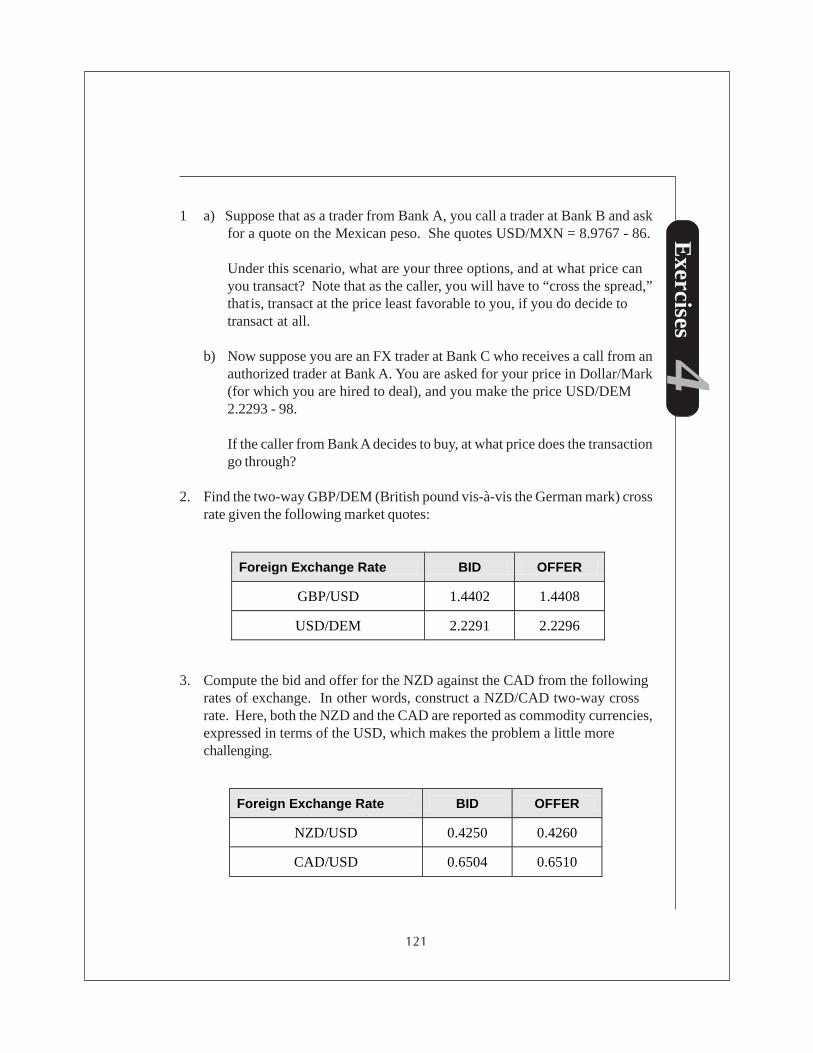
121
Exercises
41 a) Suppose that as a trader from Bank A, you call a trader at Bank B and ask
for a quote on the Mexican peso. She quotes USD/MXN = 8.9767 - 86.
Under this scenario, what are your three options, and at what price canyou transact? Note that as the caller, you will have to “cross the spread,”thatis, transact at the price least favorable to you, if you do decide totransact at all.
b) Now suppose you are an FX trader at Bank C who receives a call from anauthorized trader at Bank A. You are asked for your price in Dollar/Mark(for which you are hired to deal), and you make the price USD/DEM2.2293 - 98.
If the caller from Bank A decides to buy, at what price does the transactiongo through?
2. Find the two-way GBP/DEM (British pound vis-à-vis the German mark) crossrate given the following market quotes:
Foreign Exchange Rate BID OFFER
GBP/USD 1.4402 1.4408
USD/DEM 2.2291 2.2296
3. Compute the bid and offer for the NZD against the CAD from the followingrates of exchange. In other words, construct a NZD/CAD two-way crossrate. Here, both the NZD and the CAD are reported as commodity currencies,expressed in terms of the USD, which makes the problem a little morechallenging.
Foreign Exchange Rate BID OFFER
NZD/USD 0.4250 0.4260
CAD/USD 0.6504 0.6510

122
Exe
rcis
es 4
4. Fill in the missing legs (marked Ø and Ù) for the no-arbitrage spot FXquote table below. Be sure to show all your calculations.
Foreign Exchange Rate BID OFFER
AUD/EUR Ø 0.6001
AUD/USD .5254 0.5260
EUR/USD Ù 0.8770
4.5 (a) Suppose that you are a US exporter of goods to New Zealand and have aNZD receivable due in 120 days. The forward dealers are all off at amarket luncheon, and their prices are not available. However, spot andinterest rate dealers are at work, quoting the following rates:
Rates Market Two-way Price Day Count Basis
Spot FX: NZD/USD 0.4106 / 0.4116
120 days interest New Zealand 5.75 / 5.85 Actual / 365
120 days interest United States 4.00 / 4.10 Actual / 360
What exchange rate can you assure yourself for your NZD receivable?
(b) The forward dealers come back after a convivial lunch, and one of themquotes you 0.4068 /0.4078 for 120 days forward. All other data remainsunchanged. Can you take advantage of his compotation? Explain youranswer.

123

124

Part TwoDOING IT THE EXCEL WAY
125
Part Two of this book introduces you to the Excel spreadsheet system.Spreadsheets are an excellent way of organizing computations that repeatthemselves or that require a complex layout. Consequently, spreadsheets havebecome a vital tool in the world of finance, and one wonders how we ever gotalong without them! Extensive programming skills are not required to use thesetools, but you do have to remember a few basic rules and procedures. Thoughthere are other financial spreadsheet programs, Excel – produced by Microsoft –has become the industry standard. We’ll be using Excel 2000 for our discussion inthis section, but most of the functions we use here can be found in other packagessuch as Lotus© as well.
First we shall illustrate Excel spreadsheeting principles with material on fixed interestpricing, and later we’ll extend the discussion to cover complex calculations wherethe true advantage of using a spreadsheet will become apparent. It turns out thatyou can use Excel for much more than just bond pricing, and you’ll find that theprinciples learned in this section can be readily applied in later chapters on dataprocessing for financial econometrics and similar applications.
Those who are already familiar with Excel can probably just skim Part Two, perhapstaking a quick look at the examples, working through one or two, and trying to thinkup alternative ways of producing the same result. Indeed, there are often severalpaths to the end result with spreadsheets, and we certainly don’t claim to final sayin how it’s done!

126
FiveFiveFiveFiveFiveLearning by Doing
127
An introduction to financial spreadsheets
Spreadsheets are used extensively in the world of finance for performing calculations,analyses, and constructing charts and graphs. If you are a tertiary student or arealready employed in a financial role, and find you can’t deal confidently withspreadsheet programs such as Excel or Lotus 1-2-3, now is the time to brush up onyour skills.
This section will walk you through a simple example from the financial applicationof bond pricing. Again, we’ll be using the Excel package here, but similar instructionsapply for Lotus.
To get into the spreadsheet program, double click on the Microsoft Excel icon onyour computer. (If you can’t find this icon, try double clicking on the MicrosoftOffice icon, and look for Excel inside the folder.)
Once Excel is open, you will see an empty spreadsheet. The spreadsheet consistsof cells, organized into rows which are numbered along the left hand side startingat the top with 1 running to 66,536 at the bottom, and columns which are labelledalong the top starting on the left with A, then B, C, and so on. Each cell has adistinct address. For example, [A1] is the address of the cell in the top left corner,with [B1] next right, and [A2] directly below. A cell can contain various types ofinformation such as a number, words, or a formula which may refer to other cells.You can reference the contents of a cell by listing its cell address.
Part II. Doing it the EXCEL Way
128
Financial Modeling for Managers
5.1 Step-by-step bond valuation example
Task: Find the present value on a coupon date of the following bond.
Term to maturity = 5 yearsCoupon rate = 8.0% per annum paid semi-annuallyCurrent market yield = 7.0% per annum (discounted semi-annually)
Solution:
Begin with an empty spreadsheet (or worksheet, as it is called in Excel).
Using the mouse pointer, locate and click on cell [A2] (first column, second rowdown). Type the word Coupon in this cell and press the Enter key twice:
Enter Enter
You should now be in cell [A4]—that is, cell [A4] should be outlined in heavy blackso that it stands out as the active cell.
Type the word Principal and press Enter twice again.
Enter Enter
By now your pointer should be in cell [A6].
Type the words Time Period and press Enter.
Enter
Oops! By now some of you may have made a small mistake. For instance, if youtyped “Time” instead of “Time Period” by accident and hit the enter key, you cancorrect the problem without much difficulty. Use the up arrow key to return thepointer to [A6] (or just click on the cell [A6] again). Then press the F2 key to getinto edit mode, and fix your typo. Then simply press the enter key again.
Enter
Excel recognizes the words you have typed as text (or labels) and treats themaccordingly. For calculation purposes, Excel will assign a zero value to any cellthat contains text.

129
Chapter Five. Learning by Doing
“Time Period” will not fit neatly into the cell, so run your mouse pointer up to thetop of the column to the label row of letters just above row 1. Center the mouse onthe dividing line between column A and B. Click and (holding down the mouse key)drag the line to the right, causing row A to become wide enough to fit the words intocell [A6]. (Alternatively, simply double click on the dividing line between A and Bat the top of the column, and the column width will change automatically toaccommodate the label “Time Period.”)
Next, click on cell [B2] and type in 8%; then press Enter.
Enter
It would be helpful to show two decimal places, so click again on cell [B2]. Runthe mouse up to the formatting tool bar (the second tool bar above your worksheet),and click twice on the increase decimal format button that looks like this:
.0 .00
Cell [B2] should now read as 8.00%.
Click on cell [B4] and type in 1000000 next to the word Principal that sits in cell[A4]. Press Enter. As it stands, the number you have typed into [B4] is a bitdifficult to decipher at a glance. (Is it 10 million or 1 million?) Return the cellpointer to [B4] by using the arrow keys or by clicking on [B4] with the mouse, thenuse the mouse to click on the comma button in the format bar:
,
The number in [B4] will become more readable as 1,000,000.00
Note that you can type in the commas as you enter the number, in which caseExcel will accept them as an indication of how you wish all numbers to be presented.Similarly, because you specified above that you wanted 8.00% written with twodecimal places, Excel will “remember” this request and assume that you want twodecimal places for other values on the same worksheet.
With commas and two decimals, the number in B4 becomes too large to fit into thecurrent cell width. Excel 2000 will automatically make the column wider toaccommodate your number. Some older versions of Excel will fill the cell with aseries of hash marks, ######, indicating overflow. For versions prior to ’97, you

Part II. Doing it the EXCEL Way
130
Financial Modeling for Managers
will have to increase the width of column B as you did for column A. Click on thedividing line between labels B and C at the top of column B and drag it to the rightuntil there is enough space to show 1,000,000.00 in [B4]. (Alternatively, doubleclick on the dividing line between labels B and C and the column width will adjustautomatically.)
Now we are going to number the ten semi-annual time periods during which thebondholder will receive coupon payments. Click on cell [A9] to make it active, oractivate it by moving the cell pointer there using the arrow keys.
Type the number one (1) into cell [A9], and press Enter.
Enter
Type the number two (2) into [A10], three (3) into [A11], four (4) into [A12], andso on, through ten (10) in cell [A18], pressing Enter after each entry.
Enter
Column A should now contain the numbers 1 through 10 running from cell [A9] to[A18].
Click on cell [B6] and type the words Cash flows. Then press Enter three times.
At this point, you should have your cell pointer in [B9]. In this cell, you are goingto place a formula to calculate the bond’s first cash flow. This is how it’s done:
(1) First, to check that you are in cell [B9], look at the formula bar which liesimmediately above the column labels (A, B, C, etc.) on your worksheet. Youwill see the current cell address in the left-most section of the formula bar.Follow the rest of the instructions below, watching what appears in the formulabar.
(2) Type the arithmetic operator, = (the equals sign), into [B9], and then click oncell [B4]. (Note that you do not press the enter key yet.)
(3) Next, type in the arithmetic operator, * (shift-8), which stands for multiply, andclick on cell [B2] (still avoiding the enter key).
(4) Type the arithmetic operator, / , which stands for divide, followed by 2, andclick the enter button in the formula bar which appears as a green tick. The
131
Chapter Five. Learning by Doing
cell pointer should remain in [B9]. In the formula bar, to the right of the cellname (B9), there should now be the formula =B4*B2/2.
Two points are worth mentioning at this juncture:
(1) To finish the formula, you could have pressed the standard enter key or one ofthe arrow keys, but then the cell pointer would have moved one cell down orone cell in the direction of the arrow.
(2) You could also have simply typed the formula =B4*B2/2 into cell [B9] withoutclicking on cells [B4] and [B2], but the pointing method described above is bothsafer and faster, once you get used to it.
Excel recognizes that you have entered a formula in cell [B9], and responds byperforming a calculation and showing the answer—40,000—on the worksheet.When the cell pointer is on [B9], the formula will show in the formula bar, but onthe worksheet itself you will only see the answer, 40,000 in this case, showing in thecell.
Relative and absolute addressing
The formula in [B9] is fine as it is for that cell, but now we want to copy theformula and paste it into the five cells immediately below [B9]. We want Excel toperform the calculation of the interest cash flow as before, and report the answeras 40,000.00 in each of the cells.
Unfortunately there is a snag. Whenever you enter a formula, Excel assumes it isin relative address format. For many copy situations, this format would be fine, butnot in this case. If we copy the formula as it is written into cell [B10], the newformula in [B10] will read: =B5*B3/2. Excel will adjust the formula by the sameamount and direction that you move your cell. The result on your spreadsheet willread zero (0), which is clearly not the cash flow we want.
Hence, it is necessary to change the formula in [B9] into absolute address format,which will anchor the cell references in the formula to the cells [B4] and [B2], sothat when we copy the formula those references will stay the same.
We can edit the formula in [B9], changing the cell references to absolute addressesin the following way.
Part II. Doing it the EXCEL Way
132
Financial Modeling for Managers
Double click on cell [B9]. Using the arrow keys, move the flashing indicator withinthe formula until it is between “B” and “4” (in other words, zero in on the [B4] cellreference).
Then press the F4 key (top row of the keyboard).
F4
The cell reference will change to read $B$4, indicating it is now absolute. Movethe indicator to the [B2] reference in the formula and press F4 again. The [B2]should change to $B$2 and all cell references in the formula will now be absolutecell references. They will not change when the cell is copied.
Click the green tick % in the formula tool bar.
Copying a formula
We can now safely copy the contents of [B9] into cells [B10] through [B18] asfollows.
(1) Make sure the cell pointer is in [B9].
(2) Click the copy button in the standard toolbar (the icon depicting two sheets ofpaper just to the right of the printer button). To be sure it is the copy button,position the mouse over the button before clicking and the name of the tool willappear.
(3) Highlight cells [B10] to [B18] by clicking on cell [B10] and dragging the widecross mouse indicator through to cell [B18].
(4) Click the paste button (to the right of the copy button, with a clipboard andpaper).
Alternatively, if you are a confident rodent controller, you could do the above copyby clicking on [B9], then holding the left mouse button down, and with the smallcross (+) indicator showing at the lower right corner of the cell, dragging the mouseto [B10] through [B18].

133
Chapter Five. Learning by Doing
If you feel like giving the second copy technique a try, start by pressing the deletebutton (marked Del) to remove the highlighted data you have just entered using thepaste procedure. Then:
(1) Click on cell [B9] and release the mouse button. Now position the mouse onthe lower right corner of the cell (the mouse pointer will appear as a + sign tothe right).
(2) Hold down the left mouse button and drag the outline of the cell you haveselected into [B10] through [B18] and release the mouse.
Now you have copied the formula from cell [B9] into cells [B10] through [B18].Click on any of these cells and view the formula bar. It should show =$B$4*$B$2/2. On your spreadsheet, it will show as the value 40,000.00. This is the result wewant for all of these cells except the last one, [B18]. Here we must use the editoragain.
Double click on [B18] to edit, or get into edit mode by clicking on [B18] once andpressing the F2 key.
Extend the formula by adding +B4 at the end of the formula to include the repaymentof the principal. Use the arrow keys to move within the formula.
Press the F4 key to make +B4 an absolute reference.
F4
Click the green tick %.
All the cash flows should now be correctly represented in cells [B9] to [B18].
Calculating the discount factors
The next step in our bond spreadsheet involves calculating the discount factors toapply to the series of cash flows to obtain their values in today’s terms.
(1) Click on cell [C2] and type in the word Yield. Press Enter.

Part II. Doing it the EXCEL Way
134
Financial Modeling for Managers
(2) Click on cell [D2] and type in the yield to maturity as 7%; press Enter.
(3) Click on [C6], type the word Discount, and press Enter. Type the word Factorinto cell [C7] immediately below.
(4) Click on cell [C9]. Type the following keystrokes: =1/(1+
(5) Click on [D2] (which is where the discount rate or yield to maturity is stored),and press the F4 key.
(6) Type: /2)^ (the last character shift-6).
(7) Click on [A9], but do NOT press F4 this time.
(8) Click on the enter formula button, which appears as a % in the formula toolbar.
At this point, the formula in [C9] should read =1/(1+$D$2/2)^A9. The “^”symbol means raise to the power of, and the “A9” refers to the number of timeperiods for which you will be discounting.
As the first cash flow arrives after one time period, you must discount for just oneperiod. However, as the second cash flow arrives at the end of two time periods,you will want it to be discounted back two time periods. Leaving the cell referenceto [A9] as a relative reference will ensure the appropriate discounting when theformula is copied.
Click on cell [C9] and copy as before into cells [C10] through [C18]. You havenow completed the calculation of the ten discount factors.
Applying the discount factors
We will now use the discount factors we have calculated in cells [C9] to [C18] tovalue the cash flows in [B9] through [B18], and place the results in column D.
(1) Click on [D6]. Type the phrase PV of and press Enter. Then enter the wordsCash flows into cell [D7] below.

135
Chapter Five. Learning by Doing
(2) Click on [D9].Type in = (the equals sign). Don’t touch the Enter key yet.
(3) Click on [B9]. Then type * and click on [C9]. (Don’t touch the F4 key, as wewant all these address references to remain relative.)
(4) Click on the enter formula button (% in the formula tool bar).
Copy the formula in cell [D9] into cells [D10] through [D18]. Then click on cell[D19]. In this cell, we are going to put the total present value of the bond. Run themouse up to the standard tool bar and click on the sum sign, which is depicted bythe sigma symbol:
Σ
Check to see that it is summing cells [D9] to [D18]; if it doing so correctly, pressEnter. (If it is not summing correctly, you may need to edit the formula.)
Your spreadsheet is now almost complete. However, it could do with someformatting help to tidy it up and make it easier to read.
Highlight the cells [B9] to [B18]. Hold down the control key and highlight therange of cells [D9] to [D18]. The control key acts as an indicator to select thesecond range as well as the first. Both cell range selections should appearhighlighted. Click on the comma button in the format tool bar.
,
All the highlighted cells will now be formatted with commas.
Finally, click on cell [D19] and then run the mouse up to the formatting tool baragain to click on the dollar sign to the left of the comma.
$
This action puts a dollar sign in front of the number and helps to emphasize that it isa total. (Recall that you may have to adjust the column width for older versions ofExcel.)

Part II. Doing it the EXCEL Way
136
Financial Modeling for Managers
Printing and saving
Now we will print your masterpiece, but before we do that, we need to save it.
To save for the first time, run your mouse up to the menu bar which holds thevarious Excel pull-down menus such as File, Edit, View, etc. Click on the Filemenu and select the Save As... command (by clicking once again). A dialog boxwill open (the three dots, or ellipsis, always indicates that a dialog box accompaniesthat selection).
Type a suitably descriptive name in the File name box, so that you’ll rememberwhat this file contains when you come back to it in the future.
You may want to keep your files organized by saving your spreadsheet on a driveor in a folder other than the default; if so, click the drop-down button for the Savein list box, click on the disk drive you want to use, and then click the appropriatefolder.
When you are building your worksheet, it is a good idea to save your documentoften. That way, in the event of a power failure or an inadvertent keystroke, youwon’t lose too much of your work. Just click the File Save button in the standardtool bar. (It appears as a floppy disk button about third from the far left of theworksheet.)
Prettying up for printing
For printing purposes, it is often helpful to place a border around a table in aworksheet. Highlight the entire table from cell [A2] to cell [D19]. Run the mouseup to the format tool bar and click on the Borders drop-down list button. (The icondepicts arrow pointing down next to a box.)
or
Select a border from the options displayed. Alternatively, you can select Formatfrom the menu toolbar, then Cells…, Border, and make your choice from the dialogbox.
Leaving the highlighting in place, run the mouse up to the standard tool bar andclick on the print button. (The icon looks like a printer and is next to the Savebutton).

137
Chapter Five. Learning by Doing
Your first bond spreadsheet is now complete. Printed, it will look something likeFigure 5.1.
5.2 Do-it-yourself fixed interest workshop
Bonds: calculating their prices and yieldsıBonds are longer-term securities with original terms to maturity of greater than oneyear. For example, auction data from the June 29, 2001 issue of the Wall StreetJournal showed that U.S. Treasury bonds range from maturities of June 30, 2003to February 15, 2031.
Figure 5.1 Pricing a five-year bond
Recall that the basic features of a bond include:
1. Its denomination or face value; for example, $1,000,000.
2. Its maturity date; for example, June 30, 2003.
Coupon 8.00% Yield 7.00% Principal 1,000,000.00 Time Period Cash flows Discount PV of Factor Cash flows
1 40,000.00 0.966184 38,647.34 2 40,000.00 0.933511 37,340.43 3 40,000.00 0.901943 36,077.71 4 40,000.00 0.871442 34,857.69 5 40,000.00 0.841973 33,678.93 6 40,000.00 0.813501 32,540.03 7 40,000.00 0.785991 31,439.64 8 40,000.00 0.759412 30,376.46 9 40,000.00 0.733731 29,349.24
10 1,040,000.00 0.708919 737,275.57
$1,041,583.03

Part II. Doing it the EXCEL Way
138
Financial Modeling for Managers
3. Its coupon rate; for example, 3.875% p.a. (1.9375% semi-annually).
4. The frequency of coupon payments each year and the specific dates of eachpayment.
5. The identity of the issuer.
For U.S. Treasuries, interest is paid semi-annually from the date of issue. The dateof issue is usually the 15th of the auction month (though for some maturities, it is theend of the month). Auctions are generally monthly for shorter maturities, andquarterly for longer maturities.
Bond pricing
A bond’s value is determined by the present value of its future cash flows. Thesecash flows are:• the stream of fixed coupon payments, and• the repayment of the bond’s face value at maturity.
Recall the equation for the price of a coupon bond (P), Equation (9) from Section2.6 :
P = C + C + .... + (C+ FV) 1 + i (1 + i)2 ( 1 + i )n (1)
where C = regular coupon payment i = interest rate per compound periodFV = face value of bond n = number of interest periods
(generally use half years).
Problem 5.1
Find the price of a three-year bond of face value $1,000,000, paying 8.0% couponson a semi-annual basis, given the following interest rate scenarios.
Use Equation (1) above and a spreadsheet table for pricing the bond at a marketyield of 7.0%p.a.(a format for the table is suggested below).
Start by calculating the cash flows from the bond in the second column, rememberingto include the repayment of principal at the end of the sixth period. Then compute

139
Chapter Five. Learning by Doing
the discount factors in column three. Multiply each cash flow in column two by itsdiscount factor in column three, placing the result in column four.
The total price of the bond is given by summing column four to obtain the total ofthe PV’s of the cash flows.
Table 5.1 Pricing a three-year 8.0% bond at yield of 7.0%
(Note that if you seldom use spreadsheet programs, you will probably find it helpfulto reference Section 5.1, which provides a step-by-step solution to a similarproblem.)
When setting up the spreadsheet, remember:
(a) The bond pays a semi-annual coupon.
(b) The yield is quoted on a nominal annual basis, and it represents semi-annualcompounding. What discount rate will you use for a nominal annual yield of7.0%?
(c) For calculation purposes, yields can be expressed as decimals or in the percentformat (e.g., 9.0% or 0.0900—Excel will accept either.)
Then price the same bond at a yield of 9.0% p.a. You can copy the table to createanother one for pricing at 9.0%, or you could just add two more columns to the oneyou’ve already created.
Coupon: 8.00% p.a. Yield: 7.00% p.a.
Principal: $1,000,000
Time Period Cash flow Discount factor at yield of 7% p.a.
PV of cash flows at yield of 7.0% pa
1
2
3
4
5
6
Total

Part II. Doing it the EXCEL Way
140
Financial Modeling for Managers
Question:
Having found the price for the bond at a 7.00% yield and at 9.00%, what relationshiphave you demonstrated between the price of the bond and the market yield?
A bond’s coupon payments form an annuity; thus, the value of any bond is given asthe present value of this annuity added to the discounted amount of the face value.
Using the annuity formula (see Section 2.6), we can short-cut the lengthy calculationsas follows:
( )nnii
FVPVIFACP
++×=
1,
where thePV of an annuity for n periods at rate i is:
( )i
iPVIFA
n
ni
+−
=1
11
,
Table 5.2 Pricing a three-year 8.0% bond at yield of 9.0% p.a.
Coupon 8.00% p.a. Yield 9.00% p.a.
Principal 1,000,000
Time Period Cash flow Discount factor at yield of 9.0% p.a.
PV of cash flow at yield of 9.0%
1
2
3
4
5
6
Total

141
Chapter Five. Learning by Doing
Problem 5.2
Find the price of a ten-year bond of face value $1,000,000 paying 8.0% p.a couponson a semi-annual basis, given the following interest rate scenarios. This time, buildyour spreadsheet using the annuity formula. You can probably build the threeinterest rate scenarios into the same spreadsheet, since the annuity formula willshortcut the number of lines in the calculation considerably.
Market yields:
(a) 7.0%(b) 8.0%(c) 9.0%
A possible layout for the table is seen in Table 5.3.
Questions:
1. On the ten-year bond in Problem 5.2, what did you notice about the price of thebond when the yield was 8.0%?
2. Try adjusting your spreadsheet from Problem 5.1 by substituting an 8% yield(or better yet, adding extra columns to incorporate this sensitivity). What is theresult?
Table 5.3 Pricing a ten-year 8.0% bond at yields of 7.0%, 8.0% and 9.0%p.a.
Coupon: 8.0% Principal: $1,000,000
Yield Coupon flow PV of coupons PV of principal Total PV
7.0%
8.0%
9.0%
3. Can you begin to form a basic proposition from this result and the one abovefor the ten-year bond?

Part II. Doing it the EXCEL Way
142
Financial Modeling for Managers
Bonds at a premium, discount or par
A bond whose price (P) exceeds its face value (FV) is said to be priced at apremium. A bond whose price is less than its face value is priced at a discount. Ifa bond’s price is equal to its face value, then the bond is priced at par.
Problem 5.3
Make a summary table like the one below using the results of the previous twoproblems and marking the last column P (premium), D (discount), or Par (facevalue = price).
Table 5.4 Summary of results for problems 5.1 and 5.2
Price vs. face value Relationship of C to i
Discount P < FV
Par P = FV
Premium P > FV
Bond Coupon Yield Face Value Price P, D, or Par
3-year bond 8.0% 7.0%
8.0% 8.0%
8.0% 9.0%
10-year bond 8.0% 7.0%
8.0% 8.0%
8.0% 9.0%
Table 5.5 Coupon, yield and bond price
143
Chapter Five. Learning by Doing
Coupon: 8.50% p.a. Yield: ? % p.a.
Principal: $1,000,000 Target Price: 106.35
Time Period Cash flow Discount factor PV of cash flows
1
2
3
4
Total Total PV of Cash flows
PV per $100 face value:
Bond Pricing: Relationship between coupon rate (C), yield (i), andprice (P)
Now you can use the results above in Table 5.4 to summarize the relationshipbetween the bond’s coupon, the market yield, and the price of the bond. You couldset out your findings in a table like Table 5.5 , filling the third column with thecoupon and yield relationship (that is, C is either = , > , or < i ).
Note that the relationships you have revealed only hold when the bond is priced ona coupon date. When there is less than six months to run until the next coupon isdue, a bond’s price may be greater than its face value, even though the coupon rateis the same or even less than the yield.
Finding the IRR given the price of a bond
In most of the world’s interest rate markets, bonds are quoted on a price, ratherthan yield basis. If we are given a bond’s price, how can we calculate its IRR oryield to maturity?
Problem 5.4
Find the yield to maturity for a two-year bond paying a semi-annual coupon of8.5% p.a. when the bond is quoted at a price of 106.35 per $100 face value.
Using a spreadsheet program such as Excel, we can set up a table similar to theone we used in Problem 5.1 and employ one of Excel’s built-in financial functions—
Table 5.6 Finding the IRR

Part II. Doing it the EXCEL Way
144
Financial Modeling for Managers
IRR. It will perhaps be more instructive, however, to build our table as before withjust two small changes: a cell near the top to contain a target price, and a cell at thelower right to calculate current price per $100 of principal.
We can adjust the yield input (see the last column on our table) until the totalpresent value of the bond’s cash flows per $100 of principal is equal to the “target”price. The advantage of building the spreadsheet this way is that we can readilysee the relationship between price and yield. When you start inputting a guestimatefor yield, will your first attempt be above or below 8.5%?
Note that if you would like to try Problem 5.4 using Excel’s IRR function, you willhave to add another cash flow for time period 0, the settlement amount you pay outfor the bond(remember that the price is the amount you are paying to receive a setof future cash flows. So enter the price as a negative and all other cash flows aspositives). You won’t need to calculate the discount factors or PV’s of cash flowsas Excel will do that (invisibly) for you. Using the IRR function will return you theyield to maturity on an effective semi-annual basis. You will have to multiply theresult by two to obtain the nominal annual yield, that is, to get back to the standardway that bond yields are stated.
Time out for some market jargon...and a useful concept: the PVBP
When you performed the calculations for Problem 5.1, the yield was moved by onepercent at a time. For example, you calculated the price of the bond at 7.0% andthen at 8.0%. This one percent change comprises 100 basis points. If rates move,say, from 7.0% to 7.10%, we describe this as a yield increase of ten basis points.A rate increase from 7.10% to 7.11% is a move of just one basis point.
For purposes of calculation, we frequently represent yields in decimal format, sothat 7.10% appears as 0.0710 and 7.11% is written as 0.0711. In other words,0.0001 represents one basis point.
The price value of a basis point (PVBP) is the measure of the change in the priceof a financial instrument such as a commercial bill or a bond (or a futures contract,etc.) when its market rate of interest moves by one basis point.

145
Chapter Five. Learning by Doing
Problem 5.5
(a) You have already priced the three-year bond in problem 5.1 at 7.0% p.a. Tryincreasing the yield by one basis point and pricing again. That is, find the priceat 7.01% p.a.
(b) Find the difference between the values at these two yields. This difference isthe PVBP of the instrument at a yield of 7.0% p.a.
(c) Try the same exercise with the ten- year bond. What do you notice about thePVBP this time?
(d) Compare the PVBP’s of the three-year and ten-year bonds. What relationshipcan you hypothesize?
Bond Pricing – less than one discounting period from the next coupon(See Section 2.6)
In the real world, you typically do not buy a bond at one second after a couponanniversary date, so it is usually necessary to use fractional discounting when pricingbonds. Section 2.6 discusses this issue further. Equation (11) from Chapter 2,employing fractional discounting, is reproduced below as (2).
( ) ( )
++
+=
+
=
= +∑
nb
a
nk
k kb
a
i
FV
i
CPV
110 (2)
A full description of the terms of the formula is provided in Chapter 2.
Remember that the fraction b
a allows for part period discounting.
For Problem 5.6 below, you will need to use the closed form for (2) which isreproduced as Equation (3) below:
( )[ ] ( )[ ]ninib
aPVIFFVPVIFACiPV ,,11 ×++××+=
−(3)

Part II. Doing it the EXCEL Way
146
Financial Modeling for Managers
Further complicating the issue of bond pricing is the fact that Equations (2) and (3)provide the invoice price, but not the quoted price. However, these equations willsuffice for the next problem, which asks for invoice price.
Problem 5.6
If time permits, try to find the settlement price of the November 15, 2006, T-Bondstock which carries an 8.0% p.a. coupon when the current market yield is 4.04%p.a. Use September 24, 2001 as the settlement date.
(a) What are the semi-annual coupons per $100 face value?
(b) How many full coupon periods are left to run?
(c) How many days are there from settlement date to the next interest date?
(d) Calculate the number of days from the last interest date, May 15, 2001, to thenext interest date, November 15, 2001.
(e) What is the yield applied for discounting?
You will need to answer these questions before you can price the bond.
For a challenge, try to put this question onto a spreadsheet. The hardest parts toprogram in a general format are (b), (c), and (d).
If you want to get very professional, note that bonds become ex-interest ten workingdays before a coupon date. You could include a calculation for whether the bond isex- or cum-interest for the settlement date specified.

147

148

Part ThreeSTATISTICAL ANALYSIS
AND PROBABILITY PROCESSES
149
This section of the book is about statistics and probability. Roughly speaking, statisticsis concerned with the analysis of data, and probability with what we should expectthe data to reveal, based on an underlying model of how the world works. Financialeconometrics represents a fusion between the two. Also, the modern theory ofderivatives pricing utilizes models of asset prices or returns that follow dynamicpaths through time that incorporate random behavior. To understand these models,we have to know a bit about stochastic processes, which again incorporate somebasic ideas about probability.
This part of our book attempts to put all these concepts on an operational footing.Needless to say, a lot of reading can be done on the subject, from basic texts oneconomic statistics to journal articles on the latest technological gimmicks. Evenbooks on elementary statistics for business and economics cover statistical theoryin more depth than we will here. However, some statistics textbooks lack some ofthe important interpretive dimensions for financial management, and as a result,there is still much misunderstanding among practitioners and academics about ratherimportant subtleties. Some of these subtleties would take extensive explanation—not to mention technical background—but the gist can be given in more or lesseveryday language.
Before we proceed, however, another word in preparation. From now on, you aresupposed to be fairly conversant in Excel, and this expertise will now be integratedwith the text, rather than being set apart. However, we will still provide step-by-step instructions for the implementation of various data manipulations. In additionto illustrating the quantitative techniques, the information will increase your fluencyin Excel as well.
To produce histograms like those shown in Chapter 6.3 and perform regressionanalysis as we did in Examples 7.3, 7.4, 7.5 and 8.1, it will be necessary to have theExcel Analysis Toolpak (a standard Excel add-in) up and running on your computer.(From the Tools menu, select Add-Ins... and click on the check-box for AnalysisToolpak.)

150

SixSixSixSixSixStatistics Without Becoming One
151
This chapter is about statistics, though it does introduce the reader to some basicideas on probability as well. Primary emphasis, however, is on data exploration andthe principles that govern what we can reasonably infer from the data, an areaknown as statistical inference. We shall also take this opportunity to introduceyou to the art of downloading data in a format that you can use for your statisticalnumber crunching. You may find this useful even if you have no intention of doingstatistics, but simply need the data for other purposes.

Part III. Statistical Analysis and Probablity Processes
152
Financial Modeling for Managers
6.1 Notation and definitions
Density function The frequency histogram, or in theory, a function where thearea beneath the curve and between two points on thehorizontal axis represents the probability of getting valuesbetween those two points.
Distribution A general term applied to either the distribution function orthe density function of a random variable or set of randomvariables.
Distribution function The cumulated frequency histogram or density, a functionwhose height at any point is the probability of getting valuesof the random variable less than or equal to that point.Sometimes we talk about an empirical vs. a theoreticaldistribution function. The difference is that the former isderived from a sample taken from the population while thelatter is derived from the population.
Generation process Underlying real world model that generates the observeddata, especially in a dynamic context.
Kurtosis A measure of whether the shape of a given probability orfrequency density is flatter than a comparable normal densityshape. The distribution is leptokurtic if its peak is sharperand its tails are fatter than the normal density. The oppositeis called platykurtic.
Mean The arithmetic average, or in theoretical work, the sum ofthe variables’ values weighted by the probabilities of gettingthose values (in this context called the expected value orexpectation).
Moment The average or expected value of the deviations from themean raised to any designated number, usually a positiveinteger. The mean is the first order moment and the varianceis the second order (power two) moment.
Population The assumed parent set of observations from which thesample is drawn.

153
Chapter Six. Statistics without Becoming One
Random sample A sample drawn from the parent population according tosome process which assigns each observation an equalprobability of being drawn (technically, a simple randomsample).
Sample A subset of observations taken or drawn from a parentpopulation which itself may be too large, expensive orotherwise difficult to study, usually by means of some sortof randomization device to ensure that it is a representativesample.
Skewness The extent to which a frequency histogram or probabilitydensity is asymmetric. The density is positively skewed if ithas a longer tail to the right than to the left.
Standard deviation A statistic used as a measure of the dispersion or variationin a distribution. Equal to the square root of the averagesquared deviations from the mean.
Statistic A number computed according to some rule from the set ofobservations on one or more random variables.
Variance The square of the standard deviation, or the average sum ofsquared deviations from the mean.
6.2 Introduction to data
Data is where the story begins for this chapter. It comes in every shape and form,and can generally be divided into three categories: good data, not-so-good data, andtruly bad data. Before you spend any time working with a set of data, it is imperativethat you first consider whether it is appropriate for the intended purpose. If you arein the position to generate your own data, it pays to spend some time (and perhapsmoney) determining exactly what your purpose is and what kinds of claims andinferences you need to be able to draw from your data. For example, if you havesurvey data, you might ask whether it is free from selection biases. Questionnairesare notorious for containing bias; even where the response rate is good, there areissues of neutrality with respect to the dimensions being studied.
For our purposes in this chapter, we will sidestep these concerns and use dataprovided specifically for this text on the Authors Academic Press (AAP) website(see www.AuthorsAP.com). On the AAP website, you will find a database of

Part III. Statistical Analysis and Probablity Processes
154
Financial Modeling for Managers
monthly returns in two files called “USdata.txt” and “USdata.xls.” Don’t worryyet about trying to open them. The files contain monthly returns on the following:
1. A set of 14 large companies of which 13 are quoted on the New York StockExchange and one, namely York Research, is on the NASDAQ. (Notnecessarily a representative set.)
2. The S&P500 Gross index.
3. The US 30-day CD rate (reported on a monthly effective yield basis to bemore directly comparable with the other returns given).
4. Gross Return on US ten-year Treasury Bonds.
The data is nicely lined up over the period March 1996 – January 2001, to give 59observations, for each of which the returns on stocks, market index, CD rate, andbonds refer to the same number of business days. This type of data is referred toas non-overlapped, because the figure for each month is the return over that month,with no contribution from the previous month. You could, for instance, haveconstructed a much longer sequence over the same span by adopting a 30-daymeasurement frame that moves along one day at a time. This would result inoverlapped data, as successive observations would share, say, 28 days each.
The returns data is constructed in terms of what are called accumulation indexes,of which they are percentage changes. This is a way to allow for the effects of theelements of reward from holding a stock—i.e. things like dividends, rights issues,bonuses, stock splits and so forth. The basic idea is that you start with one unit ofthe stock and plough back all the reward elements into purchases of further units,at market prices: the accumulation index is the value of the fund that you end upwith at the stated point in time. The S&P500 Gross index is this kind of accumulationindex.
6.3 Downloading data
Downloading data should in theory be an easy task, but in practice you will sometimesrun into difficulties because your data source, whatever it is, may not be in Excelformat. If this is the case, you can frequently download it in an alternative formatcalled a text file, which corresponds as closely as you can get to ordinary typingformat. What we shall do in this section is to give you some directions fordownloading from a text file. Downloading from an Excel file is straightforward, soif you think that you will never have to use text file format just skip Section 6.3.You may find our treatment of the text file downloading useful for other purposes:
155
Chapter Six. Statistics without Becoming One
For example, some of the older statistics packages do not allow you to feed in dataas an Excel file, but do accept text files (often written with the suffix *.txt).Downloading or feeding in via text is a bit of a hassle because it will not easily allowyou to feed in variable names as well as the actual data (easy with Excel). So youhave to keep on your toes a bit.
As usual we shall follow a learning by doing path. The first thing to do is examinethe US data files on the AAP website. You will see that there are two files:“USdata.txt” and “USdata.xls.” We will pretend that the second file does not existand create it from the first, which is a text file You may notice another file called“Names.xls” that holds the names and descriptions of the 14 companies, in order oftheir appearance in the data.
The data comes in the form of a matrix. Each line represents an observation (onetime point) on all the variables, the first being the CD rate, the second the S&P500(or market rate), the third, the 14 companies, and finally, the return on the Bondindex. Thus, the data is presented in a matrix of 59 rows and 17 columns. Eachcolumn represents the entire set of observations on one of the variables. Each rowis a snapshot taken at some point in time of the returns on all the variables.
If you download the “Usdata.txt” file, it will appear on your directory as an iconmarked “USdata” which looks like a spiral-bound notebook. By double clicking onthe icon, the contents of the data file can be displayed. The file has been createdas a text file, which means that the observations have been entered one by one,with a tab between each figure to “delimit” it—that is, to set it apart from the onesaround it—and a hard return at the end of each line. Text files are a good way tocapture data if you are not sure what software package will ultimately be used toprocess it, because most packages will recognize a text file. We are going toconvert this data to an Excel file here, nicely labelled and formatted for readability(just like the one on the website, but don’t cheat just yet!). Here’s how to proceed.
Left click on the Excel icon to start up the program. Excel will produce a freshworkbook with the title bar at the very top showing “Book 1.” Check that the cellpointer is in the top left corner of the worksheet on the cell [A1], then run themouse pointer up to the menu bar and click on File, then Open. This will generatea dialog box which you can use to import the “USdata” text file. Beginning at thetop left of the dialog box, click the drop down button to the right of the drop downlist marked Look in: and click on the directory where you have saved the text file.Then at the bottom left of the dialog box, click the drop down button by the listmarked Files of type:, and select All files. Next, select the “USdata” notepad filefrom the large list box above, and finally, to complete your selection and close thedialog box, click the OPEN button near the bottom on the right side.
Part III. Statistical Analysis and Probablity Processes
156
Financial Modeling for Managers
If these steps have been executed correctly, pressing the open button will havestarted up a new routine called the Text Import Wizard, with a series of three step-by-step dialog boxes.
For Step 1, click on the radio button, Delimited. Then check that the next boxindicates Start import at row 1. If this box does not show “1”, then using themouse, click on one of the spinner buttons to the right, using the down arrow todecrease the number to 1, or the up arrow to increase the number to 1. SelectWindows (ANSI) from the list box to the right and press the NEXT button at thebottom.
For Step 2, select % Tab as the delimiter, and click on the NEXT button near thebottom of the dialog box.
For Step 3, select the General Column Data Format, and then select Finish. Thislast step will cause the data to be imported to your new workbook. At the sametime, a new name, USdata, will appear as the workbook title. At this point, selectFile and then Save As…, from the menu bar, and give your newly created workbooka new name of your own choice—something other than “USdata” to avoidoverwriting the existing Excel file. Click on the drop-down button for the list Saveas type:, and select Microsoft Excel Workbook. Finally, click the Save button at thebottom left.
6.4 Data exploration
OK, now we have all sorts of data. Eyeballing it won’t tell you much, and certainlywon’t provide a basis for any claims, so let’s try a bit of exploratory data analysis.To make the data handling more meaningful, it will help to begin by putting labels atthe top of your data columns. (If you skipped the previous downloading sectionand have opted to use the data as provided in Excel format, then you can skip thefollowing two sentences as well. The Excel data file from the AAP website isalready labelled.) With the cell pointer at [A1], use the mouse pointer to click in themenu bar on Insert, Rows. Then type abbreviated names in the new first rowstarting with CD rate in column A, Market in column B, IBM in column C, andso forth (taking the names in order of appearance from the file “Names.xls.”) Thebond returns appear at the end of the data in column Q.
Pick a stock at random—say, IBM—which occupies Column C of your data. Doa histogram, which is a way of summarizing the empirical distribution of returns forthis stock. We divide the horizontal axis into a number of intervals, and look at the
157
Chapter Six. Statistics without Becoming One
number of times that a return falls inside each chosen interval. Dividing this by thetotal number of observations (59) gives the relative number of times, expressed asa frequency. This is plotted on the vertical axis; the resulting construction appearsas a vertical bar chart. Of course, the whole thing will be done for us by the Excelprogram, and here is how it is executed.
With your Excel workbook containing the returns data open in front of you, run themouse pointer up to the menu toolbar, select Tools, then Data Analyses.... Again,note that the three dots indicate that there is more to follow—in this case, a dropdown list box of analysis tools. Select Histogram, and click on OK. This selectionwill cause the generation of a histogram dialog box. (This seems long andcomplicated at first, but is actually very easy when you get the hang of it.)
Respond to the histogram dialog box as follows:
Input range: Using the mouse pointer, click and drag to highlightthe third column of your data from row 1 to row60.
Bin range Skip this box, as the histogram routine will produceits own equally-spaced intervals with far lessdifficulty than you can.
% Labels Click the check box and a tick will appearindicating that option is selected.
u Output range Click the round “radio button” and type the cellname of the location on the spreadsheet whereyou wish to place the histogram. Choose a cellwell clear of the data, such as [$AA$2].
% Cumulative Percentage Click on Cumulative Percentage to select.
% Chart output Click on Chart output to select.
Then click on OK.
You may find that your chart is slightly squashed, making the interval labels on thehorizontal axis somewhat illegible. If so, click once on the chart, and you will seetiny black boxes emerge at each of the corners and mid-points of the chart border.Click and drag on the black box in the center of the lower border, stretching the

Part III. Statistical Analysis and Probablity Processes
158
Financial Modeling for Managers
Figure 6.1a IBM returns histogram
IBM Monthly Returns: March 96 - January 2001
0
2
4
6
8
10
12
14
-0.188
-0.1158
-0.0435
0.0287
0.1009
0.1732
0.2454More
Bin
Fre
qu
ency
.00%
20.00%
40.00%
60.00%
80.00%
100.00%
120.00%
FrequencyCumulative %
0
5
10
15
20
25
-0.2875 -0.2128 -0.1382 -0.0635 0.0112 0.0858 0.1605 More
Bin
Fre
qu
ency
.00%
20.00%
40.00%
60.00%
80.00%
100.00%
120.00%
FrequencyCumulative %
PG&E Monthly Returns: March 96 - January 2001
graph downward until the labels fit and can be read easily. You can produce abetter title for this chart by clicking on the word “Histogram” and typing a moreinformative phrase, such as “IBM Monthly Returns: March 1996 – January 2001.”
Figure 6.1a is our version of the IBM histogram. Of course, there is no uniquelycorrect diagram; just aim for one that looks nice and conveys the sort of informationyou want for your readers.
Figure 6.1b PG&E returns histogram

159
Chapter Six. Statistics without Becoming One
Now do the same for another stock—say, PG&E—which is stored in Column N inyour spreadsheet.
Figure 6.1b is a picture of what you might have ended up with.
Warning: When you produce additional histograms, be careful to provide adifferent output range for each selection, like $AA$25 for the PG&E stock.
Notice anything different about the two histograms?
6.5 Summary measures
Looking at the histograms in Figures 6.1a and 6.1b, you will notice some fairlysystematic differences:
(a) Returns for IBM are on average rather higher than PG&E, in the sensethat the center of the distribution – however we define this – is more to theright. Call this the central tendency dimension.
(b) The spread of observations is also wider for IBM than for PG&E or theS&P500 Gross index. Call this the dispersion dimension.
(c) The histogram for PG&E is a bit crooked; this is the skewness aspect. Inthis example, it looks as though someone has taken a nice symmetricdistribution and pushed it towards the right, thereby creating a long tail onthe left. Hence, we call this negative skewness. If the long tail is to theright, the distribution is said to be positively skewed. Although it might bebit harder for you to pick it up simply by eyeballing, IBM is also a bitskewed, in this case positively.
(d) The histogram for PG&E looks a bit peaky relative to a nice bell shape,with more weight in the center, less in the intermediate zones, and againmore weight in the end zones. The pointy head / fat tails property is calledkurtosis – specifically, leptokurtic. Rather like Dilbert’s boss.
Note that the bell-shaped property of the benchmark kurtosis comparison has atechnical name - the Normal density. More on this shortly.
There are summary measures available for all of the tendencies mentioned above.In fact, there are several measures for each of the elements (a) – (d), but we’lllimit our discussion to the following:

Part III. Statistical Analysis and Probablity Processes
160
Financial Modeling for Managers
(a) To measure central tendency, we generally use the arithmetic mean: for aset of N numbers x
1, x
2,...x
N we have:
. x N
= i
N
=i∑
1
1µ (1)
You will be used to the notation by now. Recall that the Σ is the summation sign: itmeans that you sum the observations, collectively denoted x
i, from observation
number 1 to observation number n.
The median is another widely used measure of central tendency. It is the pointwhere half the observations lie to the right (are greater than) and half to the left.
(b) To measure dispersion, we generally use the variance, written as:
( ) ( ) ( )[ ] ( ) . - x N
= xxx N
= i
N
=iN
2
1
222
21
2 11 µµµµσ ∑−++−+− K (2)
The square root of the variance, namely σ, is called the standard deviation.
Note: Often you will see the mean written as x instead of :. Likewise, in thevariance formula (2) you may see the divisor (N-1) used in place of N, while the
sample mean x is used in the formula in place of :. Indeed, this is the versionused in the Excel functions; the result is often denoted s2 or S2. These are calledsample means and variances—they indicate that the data is being regarded as nota self-sufficient population, but a sample from some extended population of actualor potential data. Sample statistics (mean, variance) are used to estimate thepopulation parameters. This is our first point of contact with the important topic ofsampling estimates, and we’ll get back to it in due course. For the practical work,go along with the Excel versions.
The variance is the “second order moment about the mean” – you can see that“second order” refers to the squares involved, and the “moment” is a measure ofpower or leverage. Notice that large deviations from the mean are squared up, orpowered up, to become of much more moment in the scheme of things – hence, thevariation aspect is increased by large deviations from the mean.
The standard deviation – sigma or σ – is another useful angle that we can call the“ballpark property.” It can be shown that at least 75% of the time, a randomvariable will lie within an interval equal to twice its standard deviation, and dependingon the precise pattern of the data, sometimes a lot closer than that. So the standarddeviation is a sort of bellwether as to how far the random variable x is likely to

161
Chapter Six. Statistics without Becoming One
depart from its mean. For most data patterns, you are not likely to find manyobservations further than one sigma from the mean, and very few more than twosigma’s away.
(c) To measure skewness, we use the third order moment about the mean:
. - x N
= i
N
=i
3
13 )(
1 µγ ∑ (3)
Again, the measures are powered up, in this case by the cube. But notice thatpositive and negative deviations from the mean are no longer treated the same –the cube of a negative deviation (x < :) is negative, while the cube of a positivedeviation (x > :) is positive. So, if the histogram is nicely symmetric about themean, there are as many positive as negative deviations, and they balance out tozero. On the other hand, a positive overall value for γ
3 indicates that overall, there
are bigger numbers above the mean than below it: the distribution is positivelyskewed. The same principle applies to negative skewness.
(d) To measure kurtosis, we proceed as follows:
First compute the fourth order moment about the mean:
. ) - x ( N
1 = 4
i
N
=1i4 µγ ∑
Then compute the kurtosis measure as:
kurt. = γ4 / σ4 (4)
Justifying this one is a bit less intuitive. It turns out for the ideal bell-shaped distribution(the normal density) that we used as a benchmark, the ratio in (4) turns out tohave the value 3. Distributions that are peaky in the middle and fat in the tails(relative to the benchmark) have kurt > 3, while those that are fatter in the middleand skinnier in the tails have kurt < 3. Often the deviation (kurt - 3) is in fact usedand one simply observes whether it is positive or negative. This is essentially thecase in Excel, where you just note whether the measure is positive or negative. Ifit’s positive, the distribution is called leptokurtotic or leptokurtic; if it’s negative,platykurtotic or platykurtic.
Once again, the issue of sampling arises. Sample data helps you estimate skewnessand kurtosis in the population. In this case, you have to make some adjustments,typically involving divisors differing a bit from N. As the sample size gets larger,the difference from N gets smaller. As we noted before, Excel functions assume

Part III. Statistical Analysis and Probablity Processes
162
Financial Modeling for Managers
the sample framework, and in the case of kurtosis, Excel uses the deviation fromthe normal benchmark of three to give a positive or negative outcome.
Hands-on example
Try computing all the above measures for the stocks you have chosen, using Excel.First, let’s compute the means.
(i) Computing the means.
Start by moving the pointer to an area of your worksheet well clear of yourdata and histograms; for instance, to cell [AM3]. Type the word MEANin [AM3] and press Enter. Then calculate the mean (or arithmetic average)for each of the sets of data used in the histograms.
Excel has a statistical function which can do this for you. In cell [AP3]type AVERAGE(C2:C60) and press Enter. You have just computed themean return for the IBM stock for the data period.
Alternatively, you can perform the same calculation using Excel’s FunctionWizard. Run the mouse pointer up to the standard toolbar and click on thefx button, which will generate a dialog box. Select “Statistical” from theFunction Category list box, and “Average” as the Function Name. Thenclick on OK, type the range as C2:C60, and click on Ok again. (Note thatinstead of typing the range, you could have also selected those cells in yourworksheet using the mouse or cell pointer.)
To produce the mean of a second series, you can simply copy the formulayou have just created and paste it to the cell on the immediate right, usingthe cut and paste buttons in the standard toolbar. (Again, passing themouse pointer directly over a toolbar button will reveal its name if youneed a prompt.)
You could copy the formula into the next cell to the right for PG&E, butthen you will have to edit the formula. Press the F2 key and change thecell range selection to N2:N60 to obtain the PG&E data.
(ii) Computing dispersion, etc.
Excel has functions to compute the variance (VAR), skew (SKEW), andkurtosis (KURT), all of which can be called into action using the Function

163
Chapter Six. Statistics without Becoming One
Wizard. The desired function can be selected by clicking on the fx button,selecting Statistical as the function category, and selecting the requiredfunction name. Try this for the two selected stocks. You can incorporateall the measures into a table, with the variance, skew and kurtosis for agiven stock appearing in the same column in the cells below the mean.
Finally, you can extend the work you’ve done by doing two more series. Wesuggest you use market returns and bill rate, to see whether they look differentfrom the individual stocks. For the additional histograms, you can use the outputrange $AA$50 and $AA$65 for the two new selections.
To do the summary measures for the additional selections, you can simply copy allfour measures for IBM and paste them across into the cells in the two columnsdirectly to the left of the IBM calculations. (This copy and paste action willautomatically result in the selection of the correct data—the data from Columns Aand B of your spreadsheet.)
The result of applying the four Excel functions to the four variables is displayed inTable 6.1 below.
Table 6.1 Summary comparison
The results for IBM and PG&E conform to the conclusions we made earlier byeyeballing the histograms. For example, we see that PG&E is indeed negativelyskewed, and IBM is positively skewed. PG&E is distinctly leptokurtic, while IBMis platykurtic (recall that Excel measures this from the zero base). You will noticesome differences when you look at the market return and the CD rate. As youwould expect, the dispersion of the market is less than for individual stocks, and thedispersion for the CD rate is quite a bit less.
CD rate Market IBM PG&E
Mean 0.004662 0.015277 0.027725 -0.001301
Variance 1.6E-07 0.002161 0.010533 0.008008
Skewness 0.852361 -0.748774 0.340452 -0.714566
Kurtosis 0.169354 1.001306 -0.040204 2.123769

Part III. Statistical Analysis and Probablity Processes
164
Financial Modeling for Managers
6.6 Distribution function and densities
Now we are going to generalize things a bit. In essence, we will re-examine thedata we have just explored, and view it as a sample from some underlying populationof security returns. The underlying population can be provisionally thought of as abig histogram in the sky—but of course, this description would not satisfy ourmathematician friends, so let’s try to place our intuition on a firmer footing.
Go back to the histogram computation in the previous section. At each interval ofthe horizontal axis, instead of simply recording the number of observations fallingwithin that interval, record the number falling less than the upper limit—that is, thenumber in the chosen interval plus the number in all the intervals less than this.Then express the result as a ratio, by dividing by the total number of observations(in this case, N = 59) and plot. This is actually what you asked Excel to do whenyou selected Cumulative Percentage while producing the histograms for the twodata series.
The result is called an empirical distribution function. The plot is cumulative innature, since at each step, we are adding in the new histogram interval to all thepreceding. We are in effect cumulating the histogram. The plot starts out at zeroand ends at one, because by then all the numbers have been included. If you turnback to figures 6.1a and 6.1b, you can see that in each case, the empirical distributionfunction is listed as “cumulative %” and superimposed on the histogram.
This perspective is the key to making further generalizations. Suppose that insteadof 59 observations, we have one thousand. You can see that we would have beenable to subdivide our histogram intervals, and still have a reasonable number ofobservations in each. When you plot the empirical distribution function (i.e. thecumulative function), it will now look much smoother, because the steps are likelyto be much smaller. You can see that if the number of observations gets very large,the curve would become very smooth. We can call this the theoretical distributionfunction. It is nice to think of the curve as continuous to emphasize the limitingprocess, but in fact it doesn’t have to be continuous – it can have sudden jumps andstill be a perfectly proper distribution function.
You might wonder what the data histogram would begin to look like. It turns outthat the histogram as such does not survive the passage to infinity. The replacementmodel is a similarly shaped curve: bell-shaped, skewed, or whatever. You caninterpret it to mean that the total area underneath the curve is one, and the areaunderneath the curve between any two points on the axis represents the probabilitythat a single observation, selected at random, will fall within that interval. This is

165
Chapter Six. Statistics without Becoming One
called the density function. For technicians, the density function represents themathematical derivative of the distribution function, or the distribution functionrepresents the integral of the density function.
Figure 6.2 Continuous distribution function and density
Figure 6.2 portrays the continuous distribution function, F(x), and the associateddensity function, f(x). The (cumulative) distribution function is now the nice smoothcurve rising from left to right and reaching one. The corresponding density functionrepresents the rate of change of the distribution function. The area under thedensity curve to the left of any point x is the probability of getting a value drawn atrandom that is less than x. This probability is given by the value F(x) of the distributionfunction.
Note that Excel has drawn the density function as a nice bell shape. The oneillustrated above is in fact the Normal density, which is defined by the formula:
���������
������� �
����
� � ��������
,
where the number e is the base of natural logarithms.
The Normal density has just two parameters, m (the mean) and s (the standarddeviation).
0
0.2
0.4
0.6
0.8
1
1.2
-2 -1.5 -1 -0.5 0 0.5 1 1.5 2
Density
Dis tribution

Part III. Statistical Analysis and Probablity Processes
166
Financial Modeling for Managers
In Figure 6.3, Excel was used to explore the effect of changing σ and the areaunder the curve for different x values. Note that as s increases from 0.5 to 1.0, thecurve flattens close to the mean and the probability increases that an observation(x) will fall somewhere in the tail—that is, further from the mean.
Figure 6.3: Variational analysis on Normal density
An especially important special case of the Normal density is where the mean isset equal to zero and the variance is set equal to one. This is called a standard (orunit) Normal density, and instead of x we conventionally use the symbol z for astandard normal variable. If you start with a variable x with arbitrary mean m andvariance s2, you can transform to a standard Normal by writing:
. - x
= zσ
µ
In the case of a standard Normal density, the area under the curve to the right of z= 1.96 is 2.5 %, and the area to the right of 1.96 and the left of -1.96 has a total of5%. The point z = 1.96 is called the 5% critical point for the Normal density.
Normal distributions and a closely related distribution called the Student’s t are ofgreat importance for testing hypotheses. Financial returns data usually aren’tNormally distributed, but as we shall see, this does not stop us from using theNormal to test hypotheses about population parameters based on sample estimates.
0
0.1
0.2
0.3
0.4
0.5
0.6
0.7
0.8
0.9
-2 -1.5 -1 -0.5 0 0.5 1 1.5 2
SD = 1.0
SD = 0.5

167
Chapter Six. Statistics without Becoming One
With these concepts under our belts, we can reinterpret our data mining of section6.4, referring to sample statistics which are used to estimate underlying populationstatistics (or parameters, as we will call them now). Once again, you will begin tosee the divisor N-1 used instead of the N used in variance formula (2), because weare now working with sample data. By replacing N with N-1 in the samplecalculation, we are correcting the s2 of the sample in order to estimate the underlyings2 of the parent population. A similar correction must be made to the denominatorsof the expressions for g
3 and g
4. However, no such correction is necessary for the
sample mean x as an estimator of the population mean, which is usually denotedby the symbol m.
The description just given essentially motivates the theoretical distribution functionand density in terms of a limiting process, as the number of observations in thesample gets large and larger. Actually, this represents a very particular view ofprobability known as the frequentist interpretation. While this view is a convenientillustrative device, it isn’t the way most financial econometricians view the world.Econometricians generally have in mind a “data generation process” (DGP), whichis a theoretical model couched at the outset in terms of probability densities. Thesemodels may never be able to generate nice stationary histograms such as we havediscussed, so the passage to infinity, as we have described it, is impossible, andclassical statistics do not necessarily apply.
Indeed, if you consider the context of our returns data, you can see why this is thecase, at least roughly. Suppose that a stock market crash and subsequent backlashhas occurred over the last several months. This is clearly a time of high volatility.Would your probability assessment of prices for the coming month be unaffectedby this recent history? Clearly not. For one thing, you would certainly change(upwards!) the s2 for your distribution of the end of the month price. By doing so,you are starting to model the conditional distribution of the end of the monthprice, given the information available to you. In other words, you are modelling theconditional distribution of p at time t, given information available at time t - 1. Thisis what econometricians are doing as well. In such a framework, the classicalconcept of a population out there somewhere is clearly inapplicable, since we reallyonly ever have one observation possible for the coming month. The classical ideaof a sample as 59 observations drawn from a parent population does have a meaning,but only in the sense of a stationary distribution that you might get by simply ignoringthe temporal structure and considering what histogram boxes the prices fall into inthe very long run (called the stationary distribution). The problem is, it does notalways exist. We’ll return to this later. For the moment, we shall continue to assumethat classical statistics does apply and consider the important topic of samplingdistributions.

Part III. Statistical Analysis and Probablity Processes
168
Financial Modeling for Managers
6.7 Sampling distributions and hypothesis testing
Now suppose we assert at a staff meeting that the average overall monthly stockmarket returns (the S&P500, say) is m = 1% and the standard deviation is σ2 =0.02. Note that we’re asserting these as population parameters in general.Somebody challenges us; his name is Thomas Dubious. Tom is visiting from ourAustralian operation, and like many Aussies, he’s a bit of a sceptic. He agrees withthe s, but says that the correct theoretical mean m is 0.7 %, much less attractive.
Let us take a closer look. Essentially, we have postulated an underlying (stationary)probability density for stock market returns with theoretical parameters m = 1%, s= 2%. For the sake of argument, we will suppose that the density itself is nicelybell-shaped (Normal), in which case those two parameters are all that is needed tocharacterize the distribution. Thomas agrees with us on the shape and the variation,but not on the mean. How do we decide who is right?
The obvious thing to do is to look at some actual observations, which we shall takehere as a random sample of stock market returns. Suppose we have been a bitlazy and taken a sample of just four observations. To estimate m we compute the
sample average, x . It comes out as x = 1.1 %. Can we claim to have proven ourpoint? Not yet. Our colleague Thomas would surely point out that our sample sizewas too small and that the average of just four observations could wobble all overthe place.
Of course, he is right. The sample mean x is itself a random variable, and it has itsown theoretical mean and theoretical variance. The theoretical mean is exactlythe same as that of the population from which you are sampling. But the varianceof the sample mean is different – it depends on the size of the sample, as well asthe variance of the population. As you would expect, the greater the sample size,the smaller the variation you would expect in the sample mean – it will wobble farless for a sample of size of one hundred than for a sample of size just four. Indeed,one can show that under pure random sampling, the theoretical variance of thesample mean is equal to the parent or population variance divided by the samplesize (denoted n here):
variance ( x ) = σ2 / n (5)
So, if s = 2% and the sample size n = 4, the standard deviation of the mean (squareroot of the variance) is 0.02/√4 = 0.01, or 1%. You can see why our assertion thatm = 1% will carry little conviction; the true figure could be our doubter’s 0.7% withan excellent chance as well.

169
Chapter Six. Statistics without Becoming One
Indeed, suppose Thomas right and the true value really is 0.7% (this condition isnow our null hypothesis.) We can work out the probability of getting the observedsample mean of 1.1% given that m = 0.7%. To do this, we use the fact that thesampling distribution of the sample mean is itself Normal. We work out the standardNormal value corresponding to x = 1.1, given a standard deviation of 1% and anassumed mean (the null hypothesis) of Tom’s 0.7%. We get:
z = (1.1 - 0.7 ) / 1.0 = 0.4
Now you can go back to Excel, and using the Function Wizard, select “Statistical”as the Function Category, then “NORMDIST” as the Function name, and clickon Next.
Then you must respond to the second dialog box as follows:
(1) on the first line next to x, type: 1.1 (then press the Tab key)(2) on the second line next to mean, type: 0.7 (press Tab)(3) next to standard_dev, type: 1 (press Tab)(4) next to cumulative, type: true (press Tab) and click
on Finish
You will find that the function returns the value 0.655422, which represents theprobability of getting an observed sample mean of up to the value 1.1. Hence, tofind the probability of obtaining an outcome of 1.1 or greater, subtract the valuereturned by the function from 1.0 (i.e.: 1.0 - 0.655422 = .344578).
You find that the probability of getting an observed sample mean of 1.1 % or higheris 0.344578 or 34.6%. Thus, Thomas could very well have been right: even withhis assumed mean of 0.7%, we still could have gotten a sample mean as high as1.1% with an appreciable probability. In statistical terms, we could say that wehave been unable to reject the null hypothesis that Tom is right, in favor of thealternative (that we are right).
On the other hand, with a sample size of n =100, you can see from a re-applicationof formula (5) that the sample standard deviation of x is now 0.02/ 10 = 0.2%.Now calculate the z score for the sample mean of 1.1% with an assumed truemean of 0.7%. You will find that z = 20, and the probability of getting a z score ashigh as this is so small that it can safely be ignored. Almost certainly, Thomas isnow wrong. Indeed, it turns out that even we have been a bit on the conservativeside (to see this, assume a true mean of 1% and find the z score for the observed1.1% on this basis).

Part III. Statistical Analysis and Probablity Processes
170
Financial Modeling for Managers
Thomas, never one to give up, has a further objection. What if our ideas about thepopulation standard deviation s – which you will remember we simply assumedwas equal to 2% – were wrong, and in fact the true standard deviation is quite a lot
higher? It is true that in this case the sampling variance of the estimator x wouldbe higher, and our conclusions would not be quite as devastating to his case.However, we can in fact estimate s2 by using the same data as we used to estimatethe sample mean in section 6.2 using estimator (2). Remember, though, to use N -1 in the denominator since it is a sample estimate of a parent parameter.
A further complication is that the distribution of the sample mean is no longerNormal, and we have to use another set of tables (the Student’s t). These areslightly more cumbersome, because the reference tables for the probabilities nowdepend on sample size. More specifically, they depend on the degrees of freedomin the data, which is equal to the sample size less one in this case. However, thereare still 99 degrees of freedom and for a number this large, the Normal table is avery close approximation to the t table, so we may as well continue to use theNormal table. (Note that though we continue to use the term “table,” these daysmost of this data is accessible through Excel functions, making it unnecessary toreference an actual table.)
Let’s proceed to estimate the sample standard deviation. We find it comes to 2.1.
So the estimated sampling standard deviation of the mean x is now 0.21/10 =2.1%. Even with this change, you can verify that with the sample of size 100, notmuch will change as far as the z score – or the t score as we now call it – isconcerned.
At this point, Thomas is out of objections, and we have won our case.
Review
Although couched in the language of classical statistics, the discussion in this chapterhas introduced some important ideas. Here are some of the topics we’ve covered.
1. The idea of an underlying population about which we are trying to makestatements was introduced. In financial research, we typically replace theidea of a population, which is inherited from classical statistics, with the notionof an underlying model or data generation process (DGP), the parameters ofwhich we are trying to estimate or examine. Nevertheless, the language ismuch the same.

171
Chapter Six. Statistics without Becoming One
2. We also discussed the idea that we can make these statements by drawingsome data from the population, or observing a more limited set of data presumedto have been generated by the underlying DGP.
3. A realization that once we use estimates based on samples, the values of thoseestimates can be expected to fluctuate depending on what numbers happen toappear in the samples – in other words, the sampling variation. This variationin sample-based estimates over different possible samples is called the samplingdistribution of the estimates.
4. The sampling distribution of our estimates governs the degree of convictionwith which we can infer things about the underlying parameters using thesampling estimates. Based on what we know about the sampling distribution ofthe estimates, we can make statements which give the probability that anyhypotheses made on the basis of the sample data are correct.
Whew! We have covered quite a bit of the territory of statistical estimation andhypothesis testing, in a very intuitive way. For the purposes of illustration, we haveused the sample mean as an estimator of a population mean. Later, we will dealwith more useful sorts of parameters and estimators with respect to financial data.But the fundamental concepts are the same, no matter what the context. In themeantime, note that all the standard estimators you are likely to use come withestimates of their sampling distributions attached. In particular, the package youuse will almost certainly give not only the estimate itself, but also an estimate of theits sampling variance. These should always be presented together, so that the readercan first look at the estimated value and then at the sampling variance of the estimateto see how likely it is to wobble around. This allows the reader to make up his orher own mind as to how much credence to give the estimate.
This is all the formal theory of sampling distributions that we need. We’ve alsotouched on the topic of hypothesis testing in the context of our debate with ThomasDubious. However, we shall leave a formal treatment of hypothesis testing to thestatistics textbooks.
172
Exe
rcis
es 6
1. Not too long ago, we saw an MBA questionnaire circulated to corporatetreasurers asking them whether they practiced formal risk managementtechniques. Would the following categories of recipients have the sameresponse rate?(a) Treasurers who do not practice risk management techniques(b) Those who do practice risk management techniques, but are too busy
and/or do not like MBA students(c) Those who are not too busy and who do practice risk management
techniques
Hence, evaluate such a questionnaire as a research tool.
2. Although we have followed convention in using the arithmetic mean of returns,for returns data, the geometric mean is often – and more correctly – used.The geometric mean g is defined implicitly by the formula:
(1 + g)N = ( 1 + x1 )( 1 + x
2 )....( 1 + x
N )
In other words, it is the constant return that would compound up to exactly thesame terminal amount as the observed sequence of returns x
1, x
2 ....x
N.
Comparative returns data are used extensively by the research firms that compilefund rankings. For such purposes, which do you think is the more correctmeasure—the arithmetic mean or the geometric mean?
3. Here are some random variables of different kinds. What sort of density shapedo you think each would have? (Look in particular at the symmetry, kurtosisangles, and whether the shape might be bimodal, meaning it might have twopeaks rather than one.)
(i) Daily stock market returns.(ii) The weights (in pounds or kilos) of the population at large.(iii) The weights of money market dealers.(iv) Incomes in the population at large.(v) The number of tourists eaten by crocodiles in Queensland each year.(vi) The distribution of grades in your class on the next exam.

173
Exercises
64. We know from the Normal tables that for a standard Normal density, prob (z >
1.96) = 0.025. Because the Normal density is symmetric, we can also say thatprob (z < -1.96) is also equal to 0.025. So +1.96 and -1.96 are the upper andlower 2.5 % critical points, making up 5 % together, so that they are sometimescalled the two-tailed 5 % points.
Assume that the distribution of a sample mean x is Normal with mean m andvariance s2/n. Use the standard Normal limits above to claim:
− n
+ x ,n
xσσ
96.196.1
Suppose you could repeatedly draw samples of size n and compute the meanof each such sample. Then 95% of the time, the interval will contain the truemean m. The above interval is said to be a 95% confidence interval for m.Loosely speaking, once we have computed the sample mean 0 we can be 95%confident that the true mean will lie between the two limits.
Getting back to our debate with Thomas, let’s look at this another way. Wedraw a sample of size four, and find a sample mean of 1.1%. We know thepopulation standard deviation is s = 2%.
(i) Find a 95 % confidence limits for the population mean of stock returns.(ii) Now change the sample size to n = 100. What happens to the confidence
limits?

174

SevenSevenSevenSevenSevenRegression and All That
175
In this chapter, we extend our discussion to consider the association between twoor more variables, rather than each one in isolation. It is important for us to do so,because many of the statements in financial theory and practice are indeed aboutrelationships. Often these appear in the form of hypothesized equilibrium properties.For instance, the famous CAPM theory concerns the relationship in a state ofcapital market equilibrium between the return on individual stocks on the one hand,and the market return, on the other. Or, when we hedge one position with another,we need a formal way of handling that vital stochastic (a fancy name for random)relationship between the hedge instrument and what is being hedged. Regressionmethodology is a window into all this.

176
7.1 Notation and definitions
Covariance The average product of deviations from means of twovariables; measures the extent to which one variablemoves along with the other (positive covariance) or inopposition to the other (negative covariance).
Correlation coefficient The coefficient of correlation between two variables;equal to the covariance divided by the product of thestandard deviations, with value lying between +1 and–1. If the two variables have no statistical association,the value is zero, while if the two variables plotperfectly along the straight line, the value is either plusone or minus one.
Degrees of freedom The effective independent dimensionality of acomputed statistic, which may be less than the numberof observations.
Histogram A bar graph of a frequency table, where the intervalsof the table plot into bars or boxes, with a base equalto the interval and height equal to the frequency.
Null hypothesis The value of a parameter given an assumed base casemodel or condition, to be accepted or rejected for thealternative hypothesis—its value under an alternativecondition.
OLS Acronym for Ordinary Least Squares, the most basicstatistical technique for fitting parameter values to aline or curve; operates by choosing the parametervalues that minimize the sum of squared deviationsfrom the assumed line or curve.
Regression The hypothesized relationship between a dependentor left hand variable, and one or more independent, orright hand variables, plus a residual disturbance termto allow for random influences.
Scatter plot or diagram A graph of data pairs with observations of one variablealong the horizontal axis and observations on the otheralong the vertical axis.

177
Chapter Seven. Regression and All That
7.2 Bivariate data exploration
Now take two of the disk series, say an individual stock of your choice (call it y)and the market (call it x). We are going to explore some measures of associationbetween them. As in classical statistics, it is convenient to imagine that the 59observations form a sample from some stationary bivariate distribution, so we shalluse the sample versions of the various estimators, which you will recall typicallyhave N-1 rather than N in the denominators, at least for second order variationalmeasures.
Before we go further, a bit of data exploration in the form of a scatter diagram maybe helpful.
Copy your data on the “Market Returns” from column B of your open Excelworksheet into another free zone on your worksheet, hitting the paste button whenyou have run the cell pointer across to, say, cell [BA2]. Copy data from column C(IBM Ltd), pasting it into cell [BB2] on down, so that it lies directly to the right ofthe market returns data. In cell [BA1], type the word Market; in cell [BB1], typeIBM. Employing the Excel Chart Wizard, we will incorporate this newly isolateddata into a scatter diagram, which has the market on the horizontal and the IBMstock on the vertical. The individual points will appear as small diamond shapes.
Move the cell pointer to the point where you want your graph, for instancecell [BC2], and with the mouse pointer click on the Chart Wizard button inthe standard toolbar to bring up the first of five dialog boxes. (Alternatively,from the menu bar, select Insert, Chart…, and proceed as follows.)
Step 1: Click on the XY Scatter Diagram to select the Chart Type. Thenselect the first format for the XY Scatter Chart (which has noconnecting lines between the data points), and click on [Next>].
Step 2: Click on cell [$BA$1] and holding down the left button of themouse, drag to cell [$BB$60] to define the data range for yourgraph. (Or simply type the range with a colon between the startand end points, but note that the range should be specified withabsolute addresses.) Check that the “Data series in:” shows asColumns. Click on [Next>].
Example 7.1
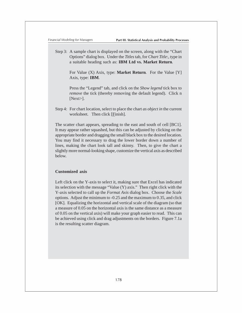
Part III. Statistical Analysis and Probability Processes
178
Financial Modeling for Managers
Step 3: A sample chart is displayed on the screen, along with the “ChartOptions” dialog box. Under the Titles tab, for Chart Title:, type ina suitable heading such as: IBM Ltd vs. Market Return.
For Value (X) Axis, type: Market Return. For the Value [Y]Axis, type: IBM.
Press the “Legend” tab, and click on the Show legend tick box toremove the tick (thereby removing the default legend). Click n[Next>].
Step 4: For chart location, select to place the chart as object in the currentworksheet. Then click [Finish].
The scatter chart appears, spreading to the east and south of cell [BC1].It may appear rather squashed, but this can be adjusted by clicking on theappropriate border and dragging the small black box to the desired location.You may find it necessary to drag the lower border down a number oflines, making the chart look tall and skinny. Then, to give the chart aslightly more normal-looking shape, customize the vertical axis as describedbelow.
Customized axis
Left click on the Y-axis to select it, making sure that Excel has indicatedits selection with the message “Value (Y) axis.” Then right click with theY-axis selected to call up the Format Axis dialog box. Choose the Scaleoptions. Adjust the minimum to -0.25 and the maximum to 0.35, and click[OK]. Equalizing the horizontal and vertical scale of the diagram (so thata measure of 0.05 on the horizontal axis is the same distance as a measureof 0.05 on the vertical axis) will make your graph easier to read. This canbe achieved using click and drag adjustments on the borders. Figure 7.1ais the resulting scatter diagram.
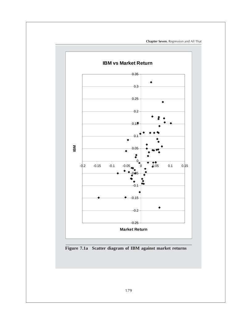
179
Chapter Seven. Regression and All That
IBM vs Market Return
-0.25
-0.2
-0.15
-0.1
-0.05
0
0.05
0.1
0.15
0.2
0.25
0.3
0.35
-0.2 -0.15 -0.1 -0.05 0 0.05 0.1 0.15
Market Return
IBM
Figure 7.1a Scatter diagram of IBM against market returns

Part III. Statistical Analysis and Probability Processes
180
Financial Modeling for Managers
You can do a similar scatter chart for another stock—say, Wendy’s—which resides in column P of your worksheet. Copy the data for the marketinto cell [BA64] and down, and the data in column P for Wendy’s in cell[BB64] on down. In cell [BA63], type the word Market; in cell [BB63],type Wendys. Run the mouse pointer to cell [BC63] and click to anchor anew scatter chart. Then proceed as above using the newly positioneddata.
Start by clicking on the Chart Wizard button and specifying the range$BA$63:$BB$122. The title for the new chart could be “Wendy’s vs. MarketReturns,” with “Wendy’s” on the y-axis and “Market Returns” on the x-axis. Again, you will probably find it helpful to customize the y-axis, thistime by specifying a minimum of (-0.2) and a maximum of 0.3. You willprobably also wish to re-size the graph by dragging the borders as with theprevious scatter diagram. Figure 7.1b reproduces a scatter diagram forWendy’s.
Modify and beautify
You might want to modify the chart title or axis labels at some time afterthe graph is constructed. For example, suppose you wish to alter the titlein the second chart above to “Scatter Diagram: Wendy’s International vs.Market.” Click (using the left mouse button) on the original title to highlightit. Then click within the title after it is highlighted and proceed to edit.
Other aspects of the graph presentation, such as borders and shading, mayalso be changed through formatting. There are two main format sectionsto your graph: the inner plot area which contains the graph itself, and theouter chart area which holds the title and axis labels. To change either ofthese zones, first click anywhere on the chart to select it.
If you wish to alter the plot area, left click within the plot area to highlightit (Excel will signal with the indicator tag reading “Plot Area”) and thendouble click the left mouse button to activate the Format Plot Area dialogbox. (Rather than double clicking, you can right click and select Format
Example 7.2
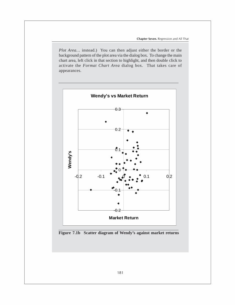
181
Chapter Seven. Regression and All That
Plot Area… instead.) You can then adjust either the border or thebackground pattern of the plot area via the dialog box. To change the mainchart area, left click in that section to highlight, and then double click toactivate the Format Chart Area dialog box. That takes care ofappearances.
Wendy's vs Market Return
-0.2
-0.1
0
0.1
0.2
0.3
-0.2 -0.1 0 0.1 0.2
Market Return
Wen
dy'
s
Figure 7.1b Scatter diagram of Wendy’s against market returns
Part III. Statistical Analysis and Probability Processes
182
Financial Modeling for Managers
7.3 Regression statistics
Now think about the following statistic:
. x - x y - y -N
= ii
N
=i
yx ))((∑11
1σ
This is called the covariance between y and x; it is symmetric so that we couldhave written it as σ
xy. Use of the N-1 rather than the N in the denominator means
that we are looking upon it as a sample estimate of a parent σyx
, so we really shouldwrite it as S
yx or something similar. However, the precise denominator turns out
not to matter in the present context.
The covariance is the sum of the deviations from the mean for each variable,multiplied together. Suppose that positive deviations for y tend to be associatedwith positive deviations in x – in other words, when x is higher than usual, so is y.Then the covariance will be positive. But if positive deviations in x tend to beassociated with negative deviations in y, then σ
yx < 0.
By itself, the covariance is not used much as an end product, but it is an essentialintermediate step for a number of statistics that are. Two such are as follows:
1. The correlation coefficient:
.
= rxy
yz
σσσ
Sometimes you will find this written as the uppercase R or as its square R2 (SeeSection 7.6).
2. The regression coefficient of y on x:
.
x - x
x - x y - y
= = b
i
N
=i
ii
N
=i
x
yx
)(
))((
2
1
12
∑
∑
σσ

183
Chapter Seven. Regression and All That
The correlation coefficient is a measure of the closeness of association between yand x. More precisely, it measures the degree to which y can be explained as alinear function of x. Thus we could write something like the following:
For each observation i,
yi = α + β
x
i + ε
i . (4)
Here, yi would be explained in terms of a linear function in x
i, which is the first part
of the right hand side. The parameter α is called the intercept, the point where theline crosses the vertical axis. The parameter β is called the slope, which measuresthe steepness of the line. For example, β = 1 would mean that y changes one forone with x. Beta could be negative, in which case the line would slope downwards.Figure 7.2 illustrates this example. The last component on the right hand side of (4)(the residual ε
i) simply represents the idea that the proposed line does not fit exactly.
If it did, for all intents and purposes, y would just be a rescaled version of x—hardlya separate variable in its own right.
If the correlation coefficient were one, then the line would indeed fit exactly. If thecorrelation coefficient is zero, then the line – any line – is simply no help at all. Ifin the latter case we plot the actual observations of y
i against x
i as a scatter diagram,
then the pattern is likely to be just a blob, with no structure. Actually, there could bea non-linear structure to the relationship, but because the correlation coefficient isjust a measure of linear associations, it would not pick this up.
The regression coefficient b is best regarded as a sampling estimate of the slopecoefficient β. Technically, it is a special sort of estimate called the least squaresestimate. This means that to fit (4) to an observed scatter diagram, you could thinkof it as trying various values of the β’s and juggling them around to end up with thevalues that minimize the squared sum of fitted residuals from the line(i.e. Σ e
i2).
As you can see in Figure 7.2, line A (i.e. α1, β1) is a much better fit than line B (α2,β2). The best fit is given by β = b, the regression coefficient, with the estimate forα defined by:
. xb - y = a
Incidentally, this relationship indicates that the line of best fit must pass through thesample mean point on the scatter diagram which is the point:
( ) . , x y

Part III. Statistical Analysis and Probability Processes
184
Financial Modeling for Managers
Can we do all of this with Excel? Of course! Let us continue with thesame data series that we used in Examples 7.1 and 7.2, namely IBM andWendy’s. In each case, we will employ the market return as the associatedvariable for the purposes of regression and correlation examples. Actually,we will see in Section 7.4 that as a financial procedure, this is not 100%sensible, but we’ll get to that in due course; for the moment our purpose ispurely illustrative.
The correlation coefficient tool is found in the menu toolbar by clicking onTools, Data Analysis..., and then selecting Correlation from the “Analysis
Example 7.3
Figure 7.2 Regression line on a scatter diagram
-0.3
-0.2
-0.1
0
0.1
0.2
0.3
-0.2 -0.1 0 0.1 0.2
0 x
y
y
εi
α1, β1
α2, β2
observation i
εεεεεi

185
Chapter Seven. Regression and All That
tools” box, and clicking [OK]. (If Data Analysis… does not show up, youwill need to select Tools, Add-Ins, and tick Analysis ToolPak, and clickon OK before proceeding with Example 7.3.)
This action will generate a Correlation dialog box for which you can nominatethe Input range [$BA$1:$BB$60], to use IBM and Market returns.
The input data is grouped by:
u Columns, with
% Labels in First Row.
For output select:
u Output Range (as) $BW$2 and hit [OK].
To do the regression analysis, slide the cell pointer over to cell [CA2] andin the menu toolbar click on Tools, Data Analysis..., and then selectRegression from the “Analysis tools” box, and click on [OK].
To continue the analysis using IBM, nominate [$BB$1:$BB$60] as theInput for the Y Range, and [$BA$1:$BA60] as Input for the X Range.Then select the following:
% Labels
For Output Options, select:
u Output Range $CA$2
For Residuals, select:
% Residuals % Line Fit Plots
Then click [OK].
The above regression analysis procedure will generate a set of statisticsand another scatter diagram with a fitted regression line. For the moment,

Part III. Statistical Analysis and Probability Processes
186
Financial Modeling for Managers
we will simply bypass commentary on the set of statistics that flashes up– we will deal with these in the extended example of the next section.
Again, it may be necessary to tidy up the diagram by dragging on bordersand adjusting the scale on either axis. You might also wish to alter the lookof the data points. To do so, left click on the plot area of the graph, andthen double click on a data point. This action will open up the FormatData Point dialog box. Select Patterns to change the look of the set ofdata points. If you have clicked on the predicted points, you can changethe shape, color and so forth of the fitted line. Or, by double clicking onone of the “IBM” points, you can use the resulting dialog box to alter thepresentation of these points.
Figure 7.3a Fitted regression line for IBM on market returns
-0.25
-0.15
-0.05
0.05
0.15
0.25
0.35
-0.2 -0.1 0 0.1 0.2
Market
IBM
IBM
Predicted IBM
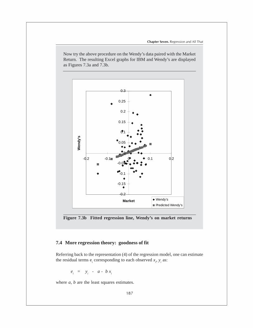
187
Chapter Seven. Regression and All That
Now try the above procedure on the Wendy’s data paired with the MarketReturn. The resulting Excel graphs for IBM and Wendy’s are displayedas Figures 7.3a and 7.3b.
Figure 7.3b Fitted regression line, Wendy’s on market returns
7.4 More regression theory: goodness of fit
Referring back to the representation (4) of the regression model, one can estimatethe residual terms e
i corresponding to each observed x
i, y
i as:
ei = y
i - a - b x
i
where a, b are the least squares estimates.
-0.2
-0.15
-0.1
-0.05
0
0.05
0.1
0.15
0.2
0.25
0.3
-0.2 -0.1 0 0.1 0.2
Market
Wen
dy'
s
Wendy's
Predicted Wendy's

Part III. Statistical Analysis and Probability Processes
188
Financial Modeling for Managers
The sum of squares SSE = Σ ei2 is called the error sum of squares, and the
quantity
( ) ( )22ˆ
22
−=
−= ∑
N
SSE
N
eiεσ (5)
is described as the fitted sigma squared. We subtract two (2) from N in thedenominator of (5), because we had to estimate two parameters, namely α and β,before we could calculate the statistic we are after. In statistics terminology, thecomputation uses up two degrees of freedom. In Excel, the fitted sigma squaredis referred to as the standard error, that is, the standard error of the equation as awhole.
One can show that:
( ) 222 1ˆ yr σσε −=
This means that the estimated error variance is just that of the dependent variable,reduced by the factor (1-r2). You will notice that if r = 1, the sum of squares of theresiduals is just zero, which can only be true if each of the ε
i is zero. The fitted line
is in fact a perfect fit, reinforcing an earlier remark to that effect.
The regression parameter of primary interest is usually the slope parameter β. TheOLS (ordinary least squares, which we have just calculated) estimator for β isthe regression coefficient b, computed automatically by the program. Because b isa sample estimator, it has its own sampling distribution. If you knew the residualvariance σ, you could compute the z score for your fitted value of the regressioncoefficient. Usually, you don’t know σ and it has to be estimated by the program;in this case, the z score is replaced by the t score and the probability tables arethose of the Student’s t distribution. However, the statistic is formally the same.
A common null hypothesis is that the true slope β is zero – which is a way ofsaying that the chosen right hand variable x (the explanatory variable) has noeffect on the dependent variable y. In this case, the t score is simply the observedregression coefficient b divided by the estimated sample standard deviation of b;the latter is printed out by the program. The resulting ratio is often loosely referredto as “the t value.” You may recall from chapter 6 that the t distribution and tablesare dependent on the degrees of freedom. In the present context, these are takenas the sample size less the number of primary regression parameters, of whichthere are two here, α and β. However, if the number of degrees of freedom isgreater than 50 or so, the z score and Normal table will do very well. A good rule

189
Chapter Seven. Regression and All That
of thumb is that if the computed t score as produced by the program is greater than2.00, it is interpreted as rejecting a null hypothesis of “no effect” in favor of onewhere there is an effect—that is, β… 0.
You can try this process on our extended Examples 7.1 – 7.3 above. We shall notdo it here, because we will be showing it in a more interesting framework in thenext section.
7.5 The CAPM beta
Now we are going to use the information above to do something useful—namely,to fit CAPM betas for the stocks in the data file. If you are not familiar with theidea of the CAPM beta, you could refer to most texts on investments, which wouldprovide extended coverage. For our purposes we will assume that you have someknowledge in this area. (Though the empirical treatment in many elementary textsleaves something to be desired.)
First, some comments on notation. Remember that we have 14 stocks, so we willnow use the index i to refer to the representative stock. Since we are dealing withobservations in the form of time series, we will reserve the index t for therepresentative observation (earlier we used i for this purpose, but here it is morenatural to reserve this for the individual stock). Our notation will be as follows:
ri,t = return on stock i for month t
Rt = return on the market for time t
rt = risk-free rate, which we shall take here as the one-month CD rate
Note that the certificate of deposit (CD) rate is not the ideal thing to use for the riskfree rate; even short dated CDs are not technically “free” either of credit risk or ofinterest rate risk. However, the existence of deposit insurance reduces credit risk,so we will stick with what is available.
The CAPM, in the form we need it, takes the form of two equations:
ri,t = α
i,t + β
i R
t + ε
it (6a)
for each stock i, and:
µi,t = ρ
t + β
i( µ
R,t – ρ
t ) (6b)

Part III. Statistical Analysis and Probability Processes
190
Financial Modeling for Managers
Equation (6a) assumes that for each stock i, there is a linear relationship betweenthe stock and the market. The parameter β is the theoretical regression (slope)coefficient, and this is supposed to be constant over the period of the sample – youwill note that it does not depend on the time index t. On the other hand, the interceptterm in (6a) cannot be independent of time. We shall see why in a moment.
Equation (6b) is the core of the CAPM hypothesis. It says that if there is a linearassociation such as the one represented in the first equation, then the stocks musttrade so that their expected return µ
i,t = E r
t at the start of period t bears a
particular relationship to the expected return on the market µR,t
= E Rt , again as of
time t. The expectations are dependent on information assumed to be available atthe beginning of period t to investors. Note that this will include the value of ρ
t
which is by definition known as of that instant – otherwise it would hardly be a risk-free rate. All this emphasizes that the distributions in which the CAPM is couchedare essentially conditional probability distributions – conditional, that is, oninformation presumed to be available to the investor at the start of time t. (Thenotion of conditionality is highly important in finance and we will come back to it inthe next chapter).
According to the CAPM, the beta from the regression, which is Equation (6a), getstransferred through to the conditional expectation of the return, which is Equation(6b). If we take expectations of both sides of the regression relationship (6a), theconditional expectation of the residual term is zero, so we have:
µi,t = α
i,t + β
i µ
R,t (6c)
Now you can use (6b) and (6c) to find that:
αi,t = (1 - β
i)ρ
t (6d)
You can see why we could not specify that the parameters of the regression (6a)could both be constant, independent of time. It’s OK for the beta but not for thealpha. This is also why you cannot estimate β
i as the simple regression coefficient
of the stock on the market, which is a mistake that is often made. Notice, however,that if you substitute (6d) in (6a), you end up with:
ri,t -ρ
t = β
i ( R
t - ρ
t ) (7)
This means that you can estimate the betas by regressing the excess returns ri,t
-ρ
t on the market excess return R
t - ρ
t, . However, you should do so without an
intercept term. Equation (7) is the time series equation of the CAPM.

191
Chapter Seven. Regression and All That
So let’s put this into action. We have picked General Motors (GM) as ourfirst stock. First we have to create new variables by subtracting off therisk-free rate (one-month CD rate) from both the GM return and the market.
For this section, it will prove helpful to create a new worksheet to holddata, and new calculations and graphs. Run the mouse pointer up to themenu toolbar and select Insert, Worksheet. To clearly label the newworksheet so that its contents are obvious at a glance, it could be given amore descriptive name than “Sheet 2.” From the menu toolbar, selectFormat, Sheet, Rename... and type, say, BETAS into the “Name” box.Then click on [OK]. It would also make things clearer at this point torename the original Sheet 1 with a suitable title such as “RETURNS.”Click on the “Sheet 1” tab at the bottom left of the work file to return to theoriginal worksheet. Then follow the above procedure (Format, Sheet,Rename... ) to give this worksheet the name RETURNS.
Our first task will be to subtract the risk-free rate for the appropriate timeperiod from each of the market returns and stock observations, and bringthis adjusted data onto the BETAS worksheet. Here is an easy way to doso.
Starting in cell [A2] of the BETAS sheet, type the character = and thenclick on the RETURNS worksheet tab which appears at the bottom left ofthe window (but don’t hit [Enter] at this stage). Now, in the RETURNSworksheet, run the cell pointer to cell [B2], type - (the minus sign), clickon [A2], and hit [Enter].
These steps will bring you back to cell [A2] of the BETAS sheet. In thiscell, you will now see the result of the subtraction operation you haveconstructed: 0.030745. In the formula bar, you will observe the expression“=RETURNS!B2-RETURNS!A2.” Run the mouse up to the formulabar, and click to the left of the “A2.” Then type a $ in front of the “A2” tomake the column part of the address absolute (but not the row part). Hit[Enter]. Next, copy the formula in this cell down to all the cells in thecolumn as far as [A60]. You have just created a set of data which showsthe market return less the “risk-free rate” for 59 observations over time.Now run the cell pointer up to cell [A1], and type the label: Market.
Example 7.4

Part III. Statistical Analysis and Probability Processes
192
Financial Modeling for Managers
Using the mouse pointer, with a click and drag action, highlight the entireset of 59 observations in column A. With the left mouse button held down,move the mouse to the very bottom right hand corner of the data so that itshows as a small black cross and drag across to column P. You will nowhave a full set of market returns, individual stock returns, and bond returnsfrom which the appropriate CD rate has been subtracted. These representour approximation of the excess return over the “risk-free rate” for eachobservation.
The scatter diagram of the excess returns on General Motors versus thoseof the market is shown as the black diamonds of Figure 7.4. Clearly thereis a line of best fit, and its slope looks to be roughly one.
Now we follow the procedures for regression analysis. Slide the cell pointerover to cell [A1] and in the menu toolbar click on Tools, Data Analysis...,and then select Regression from the “Analysis tools” box, and click on[OK].
To continue the analysis using General Motors, nominate [$C$1:$C$60]as the Input for the Y Range, and [$A$1:$A$60] as Input for the X Range.Then select the following:
% Labels
For Output Options, select:
u Output Range (and specify an area clear of the data, such as $T$1).
For Residuals, select:
% Residuals % Line Fit Plots
Then click [OK].
You will find a great deal of output, some of which has been reproduced onthe following page as Table 7.1
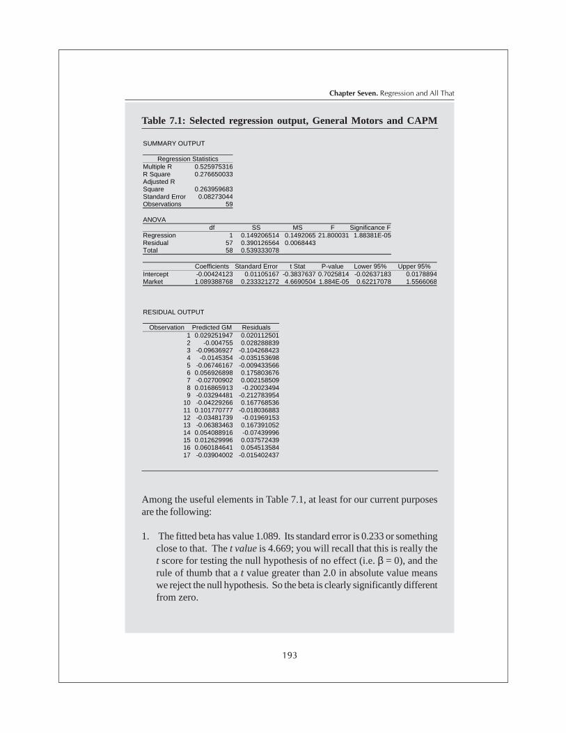
193
Chapter Seven. Regression and All That
Table 7.1: Selected regression output, General Motors and CAPM
Among the useful elements in Table 7.1, at least for our current purposesare the following:
1. The fitted beta has value 1.089. Its standard error is 0.233 or somethingclose to that. The t value is 4.669; you will recall that this is really thet score for testing the null hypothesis of no effect (i.e. β = 0), and therule of thumb that a t value greater than 2.0 in absolute value meanswe reject the null hypothesis. So the beta is clearly significantly differentfrom zero.
SUMMARY OUTPUT
Regression Statistics Multiple R 0.525975316 R Square 0.276650033 Adjusted R Square 0.263959683 Standard Error 0.08273044 Observations 59 ANOVA
df SS MS F Significance F Regression 1 0.149206514 0.1492065 21.800031 1.88381E-05 Residual 57 0.390126564 0.0068443 Total 58 0.539333078
Coefficients Standard Error t Stat P-value Lower 95% Upper 95% Intercept -0.00424123 0.01105167 -0.3837637 0.7025814 -0.02637183 0.0178894Market 1.089388768 0.233321272 4.6690504 1.884E-05 0.62217078 1.5566068 RESIDUAL OUTPUT
Observation Predicted GM Residuals 1 0.029251947 0.020112501 2 -0.004755 0.028288839 3 -0.09636927 -0.104268423 4 -0.0145354 -0.035153698 5 -0.06746167 -0.009433566 6 0.056926898 0.175803676 7 -0.02700902 0.002158509 8 0.016865913 -0.20023494 9 -0.03294481 -0.212783954
10 -0.04229266 0.167768536 11 0.101770777 -0.018036883 12 -0.03481739 -0.01969153 13 -0.06383463 0.167391052 14 0.054088916 -0.07439996 15 0.012629996 0.037572439 16 0.060184641 0.054513584 17 -0.03904002 -0.015402437

Part III. Statistical Analysis and Probability Processes
194
Financial Modeling for Managers
You could form the t score against a null hypothesis that the true valueof beta is 1.0. The t score would then be:
t = ( 1.089 - 1.0 )/ 0.233 = 0.38192
Since this is less than the benchmark critical point of 2.00 for 57 degreesof freedom, we can accept the hypothesis that the true beta is equal toone. If you formulate the test as a so-called one-tailed test, wherethe only allowable alternative hypothesis is that beta is greater thanone, then the corresponding critical value for the t distribution reducesto 1.67, rather than 2.00. Because our t value is less than this, wewould reject the alternative that beta was greater than one. Thingsbecome a little less distinct in cases where there are marginal values.
2. The intercept – the value of alpha – is -0.004. You can test the nullhypothesis that it is equal to zero – as the CAPM predicts – by formingits own t score. This is done automatically by the program to give a tvalue of -0.384, which is not significantly different from zero. Thusthis fits, so to speak, with the CAPM.
3. The r statistic is printed out as “multiple R.” We’ll explain what thismeans in the next section, but here it can be taken as the r value, andis 0.526. The corresponding r2 = 0.277, which means that 28% of thevariation in General Motors’ excess returns is explained by the market.
4. The estimated value of the standard error (which appears as the squareroot of the variance) is σε = 0.083.
Figure 7.4 below plots the scatter diagram of the excess returns, withGeneral Motors on the vertical axis and the market on the horizontal. Thefitted line is also shown.
Don’t bother too much about the rest of the output. Anova is a measure ofwhether the relationship as a whole is statistically significant. In the presentcase, the only right hand variable is the market return, and its t value will dofor our purposes. The program also prints the fitted residuals. It is a goodidea to plot them against time to see whether there is some temporal pattern.The existence of such a pattern might mitigate the view that the residualsforming the fitted relationship are purely random. In more advancedtreatments, there are formal tests for the existence of temporal relationship

195
Chapter Seven. Regression and All That
among the residuals, such as the Durbin Watson test, but this is a littlebeyond our scope here.
Overall, it appears that the CAPM does well, at least so far as GM isconcerned. The value of beta as a bit greater than one indicates a slightlyaggressive stock. This is more or less as we might expect, because GM isa car producer and might be expected to vary procyclically with the generalbusiness cycle and through this, with the market return index.
-0.3
-0.2
-0.1
0
0.1
0.2
0.3
-0.2 -0.15 -0.1 -0.05 0 0.05 0.1 0.15
Market
GM
GM
Predicted GM
Figure 7.4 CAPM graphics – GM against the market

Part III. Statistical Analysis and Probability Processes
196
Financial Modeling for Managers
Try some or all of the other stocks. What about Praxair or Wendy’s, forinstance? Can you rationalize the betas you get for these companies?
One final point: If the CAPM relationship specifies no intercept – andEquation (7) does not have one – then you should fit the equation bysuppressing the intercept. Of course, we did have an intercept in the GMcase, which is standard, but it came out as statistically insignificantnonetheless, just as we would hope. However, it is not sufficient to regardthe fitted slope parameter from such an equation as the beta. We reallyhave to fit the whole equation without the intercept, and then look at thefitted slope parameter. This can be done as follows.
Follow the usual procedure for performing regression analysis on Excel, asdescribed in Examples 7.3 and 7.4, with one small difference. Havingselected regression from the Analysis tools and specified the Y Rangeand the X Range, select:
% Labels, as usual, but in addition, select:
% Constant is zero.
Continue with your standard selection of the output options and residuals,and then click [OK]. Your resulting regression line will be forced throughthe origin. If you do this for the GM excess returns data against the market,your output will change by a small amount. Try it and see.
7.6 Regression extensions: multiple regression
Suppose we thought that variations in stock returns might be explicable in terms notonly of the stock market as a whole, but also of influences from outside the stockmarket. In financial general equilibrium jargon, we could say that the stock marketdid not span the systematic sources of influence on stock returns. For instance, wemight decide that there are two factors that affecting stock returns. One might bea general factor just for stocks. The other might be a factor that comes over fromanother market, such as the bond market. Or it could be an exchange rate factor,representing external influences on our chosen stock or set of stocks. Since wehave data for the bond returns, we can investigate this.

197
Chapter Seven. Regression and All That
We might set up the following extended version of the CAPM equation:
ri,t - ρ
t = β
i ( R
t - ρ
t ) + γ
i ( r
b,t - ρ
t ) + ε
i,t (8)
Here, everything is more or less as before, except that we have added an additionalexcess return in bonds. Again, we could include an intercept, just for the sake oftesting whether it is zero as required by the CAPM. This extended model is actuallysimilar to something called the APT model, but it’s unnecessary to develop thecomparison here.
From the interpretive point of view, the coefficient βi measures the marginal effect
on the subject stock # i, of an increase in the market excess return. The othervariable—namely, the bond excess return—is imagined to be held constant.Likewise, the parameter γ
i gives the marginal effect of an increase in the bond
excess return. Collectively, the two excess return variables on the right side of theregression equation are called the independent variables, while the left handvariable (in this case our stock excess return) is called the dependent variable.
The least squares theory we described earlier carries over almost entirely unchangedto the statistical fitting of the multiple regression model (8). For each chosen stocki, the program will compute the estimated parameters β
i, γ
i that minimize the sum
of the squared residuals. The program will print out the estimated parameterstogether with their estimated sample standard deviations.
In place of the correlation coefficient as a measure of the goodness of the fit, is amore general statistic called the multiple correlation coefficient, conventionallydenoted R or R2. It has a similar interpretation in terms of the percentage of thevariance in the dependent variable collectively explained by the independentvariables, and lies between zero and one, the latter indicating a perfect fit. There isnow an additional measure called the corrected R square, which is a somewhatartificial way of allowing for the fact that the more right hand variables you add, themore you automatically increase the closeness of fit—that is you diminish the residualvariance. Since this is an artifice of more variables, there should be a way ofdiscounting this sort of “buckshot” approach, and this is what the corrected R is allabout – it penalizes the observed fit of the relationship to compensate for the numberof right hand variables added.
Finally, you can test the fitted coefficients as before, using the t score, or if thenumber of degrees of freedom is fairly large, using the z score and the standardNormal table. The degrees of freedom are equal to the number of observations

Part III. Statistical Analysis and Probability Processes
198
Financial Modeling for Managers
Let’s try it. To perform a multiple regression using Excel, the data for theindependent variables must sit in contiguous columns. This means it willbe necessary to copy the “market returns” data into a new column next tothe US Govt bond data in column P. With the cell pointer on [Q1], type:=A1 into the cell. Then copy cell [Q1] all the way down the Q column asfar as cell [Q60]. (Make a few random checks to see that the data is thesame as that in column A.) Your data is now set up for multiple regression.
Once again, slide the cell pointer over to cell [C1] and in the menu toolbar,click on Tools, Data Analysis..., and then select Regression from the“Analysis tools” box, and click on [OK].
If you are using GM, nominate [$C$1:$C$60] as the Input for the YRange, and [$P$1:$Q$60] as Input for the X Range. Then select thefollowing:
% Labels
For Output Options, select:
u Output Range (and specify an area clear of the data,such as $T$95)
For Residuals, select:
% Residuals % Line Fit Plots
And click [OK].
Example 7.5
less the number of right hand parameters. Thus, for two right hand regressors,there are three right hand parameters (the intercept as well as the two slopeparameters), and the degrees of freedom are N - 3.

199
Chapter Seven. Regression and All That
Table 7.2 Multiple regression output for General Motors
Results
Table 7.2 represents an edited version of the Excel output for GM asdependent variable against the ten-year treasury bond return and the marketreturn as independent variables, in each case measured as excess returnsrelative to the bill rate. You will see that once the market return is there,the bond rate adds very little. Its t value against the zero alternative isstatistically insignificant. The multiple R2 goodness of fit statistic is onlymarginally better than the earlier r2 we estimated from the market returnalone. Thus, the fixed interest market in the US appears to add little, ifanything, to the explanation of variation in common stock returns, at leastfor GM.
SUMMARY OUTPUT
Regression Statistics Multiple R 0.532882707 R Square 0.28396398 Adjusted R Square 0.258391265 Standard Error 0.083042793 Observations 59 ANOVA
df SS MS F Significance F Regression 2 0.153151167 0.0765756 11.104178 8.67314E-05 Residual 56 0.386181911 0.0068961 Total 58 0.539333078
Coefficients Standard Error t Stat P-value Lower 95% Upper 95% Intercept -0.00488087 0.011125588 -0.4387069 0.6625619 -0.02716809 0.0174063Bond 0.383079606 0.506508296 0.7563146 0.4526307 -0.63157776 1.397737Market 1.094071078 0.234284002 4.6698497 1.929E-05 0.624744137 1.563398

200
Exe
rcis
es 7
1. Do scatter diagrams for the following (the first variable named should be onthe vertical axis):
(i) Bond returns versus CD returns.(ii) Bond returns versus stock market returns (the S&P500).(iii) Stock market returns versus CD returns.
Which of the various pairs appears to be the best fit?How can you explain different slopes between the diagrams?
2. (a) How might regression techniques be used for purposes of prediction?
(b) If you use regression models for this purpose, what are the likely sourcesof error in your forecast? Assume that you have to first fit the model off aninitial sample period.
3. Aptitude test: Can you be a stock analyst?
(a) Look at the company names associated with the data in the date file. Bearingin mind what you know about the way that stock returns vary according tothe cyclicity of the stock (e.g. whether the stock varies with the generalmarket, and if so, whether “more so”), give the companies a provisionalranking as to where you think their betas would be, relative to one another.(To use the appropriate terminology, b>1 is said to be an “aggressive”stock, and b<1 a “defensive” one.)
(b) Check your economic intuition by actually computing the time series betafor each of the stocks given in the data file. List the betas in ascending ordescending order, and see how closely this corresponds with your a priorigut feeling about them.
(Of course, to be a good stock analyst, you also have to be able to constantlychange your mind without batting an eye!)
4. As a CAPM exercise, you can take a different tack and look at the beta for the government bond index against the share market. Theory suggests that atleast for a pure discount bond, there should be such a beta. You could certainlytry to compute a beta for bonds overall, against the stock market, using thedata from the web site. Thus, get the excess return by subtracting the CDreturns off the bond returns and regress this on the market excess return. Is

201
Exercises
7the bond beta greater or less than one, and how might this tie in with your priorexpectations?
5. The ordered mean difference (OMD) was developed* as a technique inperformance measurement that measures how well a given fund’s return doesagainst a benchmark return. Essentially, it captures the insight of the song“Whatever you can do, I can do better,” from Rodgers and Hammerstein’sAnnie Get Your Gun (Feel free to hum along.) The following Excel exerciseutilizes the menu tools and wizards.
(i) Take one of the stocks in the disk. Tabulate the returns on the stocktogether with the return on the market at the same date. Now reorderthe observations according to increasing values of the benchmark. Next,compute the running mean of the differences, which is the progressivemoving average as you move down. The table below illustrates thecalculation. You end up with a function that you can plot against thebenchmark return (OMD as a function of R).
(ii) If the OMD function lies wholly above the horizontal axis (all values arepositive) this means that your chosen stock (or fund, etc.) is dominant overthe benchmark (market, in this case). Sell the market and buy the stock.More commonly, in a group of stocks (such as the ones on your data disk)some will have OMD schedules that slope upwards (aggressive) othersthat slope downwards (defensive). If the CAPM hypothesis is correct, allshould cross the horizontal axis at the same point. Test the CAPM usingthe stocks from your data disk by plotting all their OMD schedules on thesame diagram.
*Bowden, R.J. (2000), “The ordered mean difference as a portfolio performance measure,” Journal of Empirical Finance, 7, 195-
223.
T Table 1 Sample OMD calculation
r values R values Reordered by R running mean difference
r R
r-R OMD 0.032 0.011 -0.021 -0.045 0.024 0.0240.048 0.047 -0.026 -0.030 0.004 0.0140.028 0.018 0.004 -0.005 0.009 0.0120.004 -0.005 0.017 0.001 0.016 0.0130.027 0.008 0.027 0.008 0.019 0.014
-0.026 -0.030 0.032 0.011 0.021 0.016-0.021 -0.045 0.028 0.018 0.010 0.0150.017 0.001 0.048 0.047 0.001 0.013

202

EightEightEightEightEightIntroduction to Stochastic Processes
203
Most variables that we deal with in finance have some sort of time dimension. Forexample, think of stock prices, bond prices, or interest rates. In making any sort ofportfolio or risk management decision, the essence of the matter is what the currentvalues are and what they are likely to be in the next period or at the end of thedecision horizon. Thus, there are at least two random variables to consider: thevalue of our stock price now (or whatever the asset), and its value in the future.One could use the same name, for example “S” for the stock price, and two differenttime suffixes, such as t and t+1so that the two random variables are S
t and S
t+1. If
you think about it, the information that you use for your guessing game about St+1
would certainly include past values such as St, S
t-1, S
t-2 and so on. In other words,
we are dealing with a potentially infinite set of random variables—the values of thestock price at all times past, present and future. A stochastic process is the namegiven to such an infinite set of random variables, with time forming the indexing setwith representative element t. Moreover, time can be treated as a continuouselement, which turns out to be very convenient.
Stochastic processes form the underlying mathematical framework of modernfinance. In this chapter, we aim to give you an idea of the nature of this frameworkwithout delving too deeply into the mathematical subtleties, which at times canbecome very complex. We shall draw your attention to some of the applications –and the jargon—so that you’ll have some idea of what the quants are talking about.
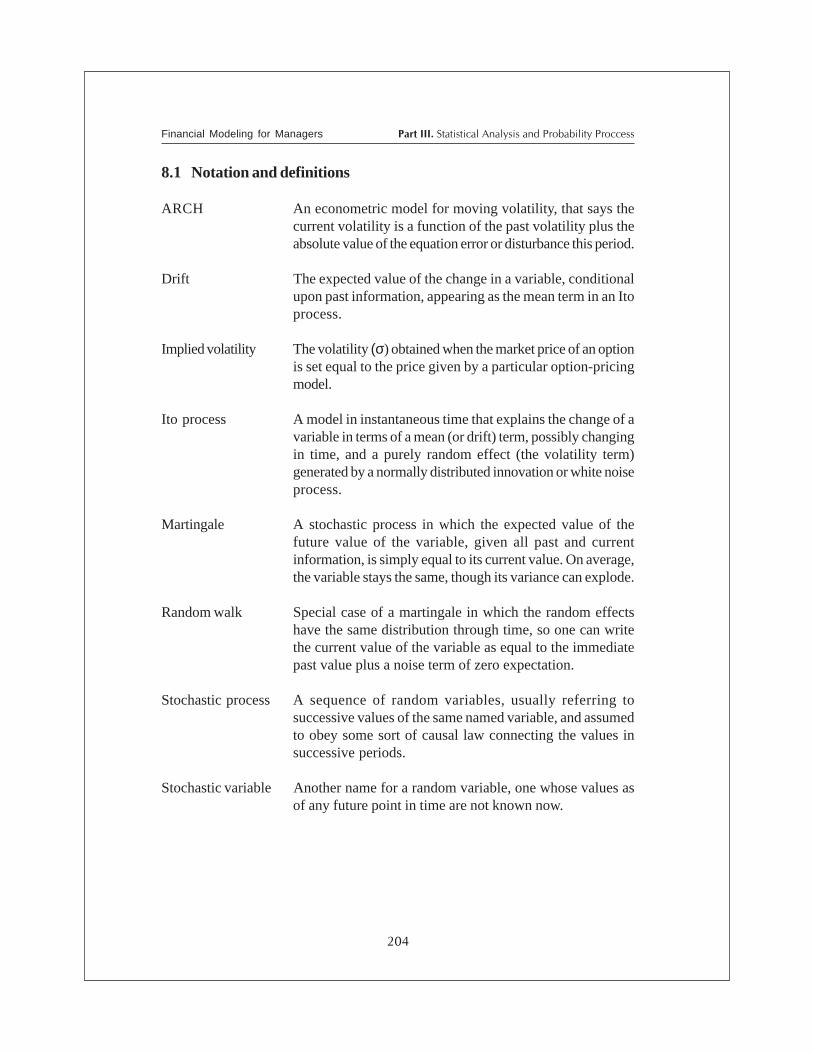
Part III. Statistical Analysis and Probability Proccess
204
Financial Modeling for Managers
8.1 Notation and definitions
ARCH An econometric model for moving volatility, that says thecurrent volatility is a function of the past volatility plus theabsolute value of the equation error or disturbance this period.
Drift The expected value of the change in a variable, conditionalupon past information, appearing as the mean term in an Itoprocess.
Implied volatility The volatility (σ) obtained when the market price of an optionis set equal to the price given by a particular option-pricingmodel.
Ito process A model in instantaneous time that explains the change of avariable in terms of a mean (or drift) term, possibly changingin time, and a purely random effect (the volatility term)generated by a normally distributed innovation or white noiseprocess.
Martingale A stochastic process in which the expected value of thefuture value of the variable, given all past and currentinformation, is simply equal to its current value. On average,the variable stays the same, though its variance can explode.
Random walk Special case of a martingale in which the random effectshave the same distribution through time, so one can writethe current value of the variable as equal to the immediatepast value plus a noise term of zero expectation.
Stochastic process A sequence of random variables, usually referring tosuccessive values of the same named variable, and assumedto obey some sort of causal law connecting the values insuccessive periods.
Stochastic variable Another name for a random variable, one whose values asof any future point in time are not known now.

205
Chapter Eight. Introduction to Stochastic Processes
8.2 Expectations
One is accustomed to see surveys of consumer “expectations” and the like, but theword will be used in a more precise sense here. The expectation of a randomvariable means its mathematical expectation, which is simply its arithmetic mean.Thus, if x
t is a random variable representing the value of a magnitude x at time t,
we write its mean as E[xt], or just E x
t for short.
We already have a rough idea of the mean from Chapter 6. The arithmetic meanof a random variable is the average value obtained by the sum of the possiblevalues, each weighted by the frequency, or probability, attached to it. In the contextof a stochastic process, the mean E x
t at time t represents the unconditional
expectation of xt at time t. Image that there is a glorious time machine that
enables you to rewind and repeat the whole history of stock market prices, overand over again. Each time you do it, there is some randomization device that saysthat you get a new time path (called a sample function in the literature). Theaverage at any specific time t of all such realized values is the unconditional expectedvalue at time t.
You might think that all this business of imagining re-runs is academic, because it isan inescapable part of our human condition that we cannot re-run time. And youwould be right – the unconditional expectation plays only a very limited role infinancial mathematics. Indeed, many of the models used to generate prices andinterest rates do not result in a finite unconditional expectation, so that theunconditional expectation does not even exist.
A more informative approach would be to ask the following: Suppose that I knowthat the stock price of a given stock yesterday was $10. Would this affect myexpectation of where the stock price tomorrow would be? Obviously, the answeris yes. Knowing today’s stock price is important information that conditions myprobability assessments of the value of tomorrow’s. Of course, there might beother information available today that also affects my probability assessments oftomorrow’s stock price – I might have learned that the NAPM (National Associationof Purchasing Managers) index has turned downwards. I might therefore extendthe information set I
t available to me today to include the state of the NAPM index,
as well as yesterday’s price, and clearly, both are useful in predicting tomorrow’sstock price. One could regard the unconditional expectation of the stock price asthe mean, with no information of any kind available. But if there is informationavailable, one could assert that in general,
E St+1
* It … E S
t+1

Part III. Statistical Analysis and Probability Proccess
206
Financial Modeling for Managers
The vertical bar is the conditioning sign. It says that the mean is conditioned byknowing the information that appears after bar. If the information set comprised S
t
and Mt , the latter representing the state of the NAPM index, one could write the
conditional expectation as E St+1
*St ,M
t .
The conditional mean, or conditional expectation, plays the central role in much offinance theory – and also in practice, as the extended example in the next sectionwill show.
8.3 Hedging
As you know by now, hedging refers to minimizing the variation in the value of agiven portfolio. For instance, if you have a receivable at the end of the comingperiod that is denominated in Canadian dollars (CAD), you might decide that youdon’t want the currency exposure. You augment the implied portfolio of CAD witha forward position in CAD, that precisely cancels out the exposure, minimizing –right down to zero – the variation in the value of your portfolio in US dollars.Similarly, if you have an exposure to the price of fine wool, you might want toaugment it with wool futures. In the first case, you can reduce the exposure rightdown to zero. In the second case you can’t, because wool futures are based on acomposite grade and the price of the futures contract will not track precisely alongwith the price of fine wool. In the latter case, one would say that there is residualbasis risk. We can also say that basis risk means that hedging is imperfect.
Suppose that your exposure is to an asset of value Y, and you have another asset ofcurrent value X available as a hedging instrument. The latter is not a perfecthedge. However, you do know that changes in their values are linearly related.Thus, the following would hold for any period t.
Let: yt = Y
t - Y
t-1( change in Y , the position value )
xt = X
t - X
t-1( change in X , the hedge instrument value )
then: yt = βx
t + ε
t (1)
We are specifying that Eyt *x
t = βx
t. In other words, once I know x
t, my expectation
of yt is equal to βx
t. This means that Eε
t *x
t = 0. The term ε
t represents a random
disturbance that separates yt from x
t, because otherwise, the two would be essentially
indistinguishable. One would simply be a rescaled version of the other. Thedisturbance has the property that knowing x
t provides no information about ε
t, so
that the latter can be regarded as irreducible variation in yt relative to x
t.
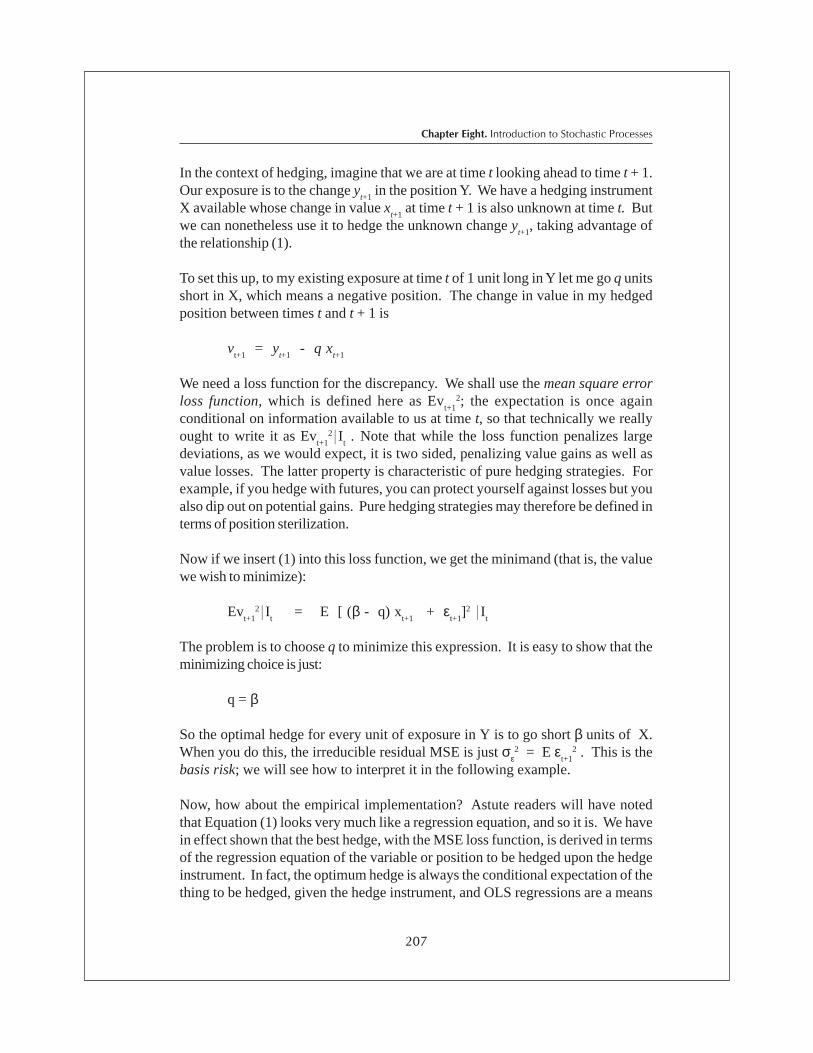
207
Chapter Eight. Introduction to Stochastic Processes
In the context of hedging, imagine that we are at time t looking ahead to time t + 1.Our exposure is to the change y
t+1 in the position Y. We have a hedging instrument
X available whose change in value xt+1
at time t + 1 is also unknown at time t. Butwe can nonetheless use it to hedge the unknown change y
t+1, taking advantage of
the relationship (1).
To set this up, to my existing exposure at time t of 1 unit long in Y let me go q unitsshort in X, which means a negative position. The change in value in my hedgedposition between times t and t + 1 is
vt+1
= yt+1
- q xt+1
We need a loss function for the discrepancy. We shall use the mean square errorloss function, which is defined here as Ev
t+12; the expectation is once again
conditional on information available to us at time t, so that technically we reallyought to write it as Ev
t+12*I
t .
Note that while the loss function penalizes large
deviations, as we would expect, it is two sided, penalizing value gains as well asvalue losses. The latter property is characteristic of pure hedging strategies. Forexample, if you hedge with futures, you can protect yourself against losses but youalso dip out on potential gains. Pure hedging strategies may therefore be defined interms of position sterilization.
Now if we insert (1) into this loss function, we get the minimand (that is, the valuewe wish to minimize):
Evt+1
2*It = E [ (β - q) x
t+1 + ε
t+1]2 *I
t
The problem is to choose q to minimize this expression. It is easy to show that theminimizing choice is just:
q = β
So the optimal hedge for every unit of exposure in Y is to go short β units of X.When you do this, the irreducible residual MSE is just σε
2 = E εt+1
2 . This is thebasis risk; we will see how to interpret it in the following example.
Now, how about the empirical implementation? Astute readers will have notedthat Equation (1) looks very much like a regression equation, and so it is. We havein effect shown that the best hedge, with the MSE loss function, is derived in termsof the regression equation of the variable or position to be hedged upon the hedgeinstrument. In fact, the optimum hedge is always the conditional expectation of thething to be hedged, given the hedge instrument, and OLS regressions are a means

Part III. Statistical Analysis and Probability Proccess
208
Financial Modeling for Managers
of identifying the conditional expectation. Then you just use the fitted coefficientsto derive the hedge portfolio. Finally, the regression estimate of the residual variancegives us the minimum residual MSE, in the sense that its square root will give usone standard deviation of the likely monetary loss remaining after the hedge. Notethat as a regression property,σε
2 < σy2 , which means that the hedged variance is
always less than the variance of the unhedged position.
These principles can apply to other situations. For instance, you could think ofimproving the goodness of fit by having a hedge comprised of two instrumentsrather than just one. To guide you to the right portfolio proportions, you would do amultiple regression of the (changes in the) position to be hedged on the changes inthe values of the two hedge instruments, as the independent variables in theregression.
Here’s an example of how it works:
Metal and futures hedge
Let us suppose that you are working in the treasury of a major munitionsproducer that uses input of copper and lead for the manufacture of bullets,shotgun cartridges and other purposes.
You have daily metals price data for the past few years. (You can find asubsection of this data, as a file entitled “copprlead.xls,” on the AuthorsAcademic Press website at www.AuthorsAP.com). The data includesdaily prices of the following:
1. Spot price of copper expressed in USD per ton2. Futures price of copper (three-month contract) expressed in USD per
ton3. Spot price of lead expressed in USD per ton
If you take a look at the data, you will see that sometimes the futures priceis above the physical price and sometimes the reverse is true. Thedifferential between the futures and the physical price is governed by severalthings, including interest rates, cost of storage, commodity shortages, etc.1
Example 8.1
1 For a well-known case where these factors changed dramatically, see one of the many accounts of Metallgesellschaft,such as Edwards, Franklin R, and Michael S. Canter “The collapse of Metallgesellschaft: unhedgeable risks, poorhedging strategy, or just bad luck?” Journal of Applied Corporate Finance, 8, 86-105.
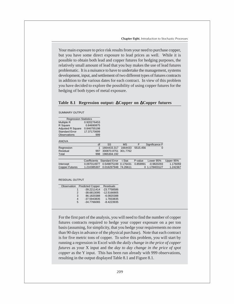
209
Chapter Eight. Introduction to Stochastic Processes
Your main exposure to price risk results from your need to purchase copper,but you have some direct exposure to lead prices as well. While it ispossible to obtain both lead and copper futures for hedging purposes, therelatively small amount of lead that you buy makes the use of lead futuresproblematic. It is a nuisance to have to undertake the management, systemsdevelopment, input, and settlement of two different types of futures contractsin addition to the various dates for each contract. In view of this problemyou have decided to explore the possibility of using copper futures for thehedging of both types of metal exposure.
For the first part of the analysis, you will need to find the number of copperfutures contracts required to hedge your copper exposure on a per tonbasis (assuming, for simplicity, that you hedge your requirements no morethan 90 days in advance of the physical purchase). Note that each contractis for five metric tons of copper. To solve this problem, you will start byrunning a regression in Excel with the daily change in the price of copperfutures as your X input and the day to day change in the price of spotcopper as the Y input. This has been run already with 999 observations,resulting in the output displayed Table 8.1 and Figure 8.1.
Table 8.1 Regression output: ∆ ∆ ∆ ∆ ∆Copper on ∆∆∆∆∆Copper futures
SUMMARY OUTPUT
Regression Statistics Multiple R 0.920276453 R Square 0.84690875 Adjusted R Square 0.846755198 Standard Error 17.37170699 Observations 999 ANOVA
df SS MS F Significance F Regression 1 1664433.317 1664433 5515.456 0 Residual 997 300870.8751 301.7762 Total 998 1965304.192
Coefficients Standard Error t Stat P-value Lower 95% Upper 95% Intercept 0.097014977 0.549875199 0.176431 0.859991 -0.9820293 1.176059Copper Futures 1.210385307 0.016297948 74.26611 0 1.178403127 1.242367 RESIDUAL OUTPUT
Observation Predicted Copper Residuals 1 -39.2211414 -23.7758586 2 -38.6813095 -12.5166905 3 86.1820388 -6.0820388 4 -37.5943835 1.7833835 5 -34.7766065 -8.4223935
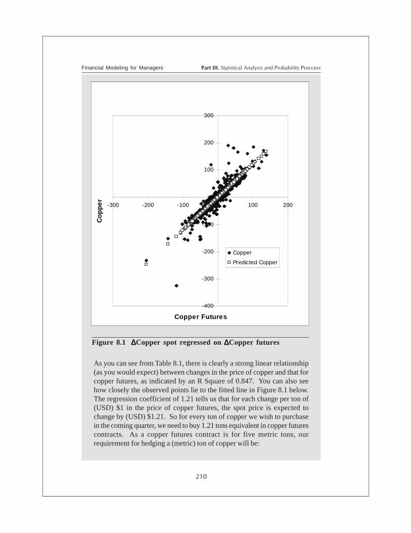
Part III. Statistical Analysis and Probability Proccess
210
Financial Modeling for Managers
As you can see from Table 8.1, there is clearly a strong linear relationship(as you would expect) between changes in the price of copper and that forcopper futures, as indicated by an R Square of 0.847. You can also seehow closely the observed points lie to the fitted line in Figure 8.1 below.The regression coefficient of 1.21 tells us that for each change per ton of(USD) $1 in the price of copper futures, the spot price is expected tochange by (USD) $1.21. So for every ton of copper we wish to purchasein the coming quarter, we need to buy 1.21 tons equivalent in copper futurescontracts. As a copper futures contract is for five metric tons, ourrequirement for hedging a (metric) ton of copper will be:
Figure 8.1 ∆∆∆∆∆Copper spot regressed on ∆∆∆∆∆Copper futures
-400
-300
-200
-100
0
100
200
300
-300 -200 -100 0 100 200
Copper Futures
Co
pp
er
Copper
Predicted Copper

211
Chapter Eight. Introduction to Stochastic Processes
number of copper futures contracts = 1.135 / (5 tons) = 0.227(a bit less than 3 contract)
The Standard Error of 17.37 indicates that with 95% probability, we expectto lose (or gain) no more than $34.74 per ton on our overnight hedgingstrategy (2 x $17.37).
For the second part of the exercise, run another regression using the one-day change in the price of lead as the X input and the one-day change inthe price of copper futures as the Y input. Again, how many copper futureswill you need?
The results of part two, using 999 observations, are given below as Table8.2 showing the summary regression output, and Figure 8.2 showing ascatter graph with fitted regression line.
Table 8.2 Regression output: ∆∆∆∆∆Lead spot on ∆∆∆∆∆Copper futures
SUMMARY OUTPUT
Regression Statistics Multiple R 0.884253491 R Square 0.781904237 Adjusted R Square 0.781685485 Standard Error 42.54337127 Observations 999 ANOVA
df SS MS F Significance F Regression 1 6469419.282 6469419 3574.386 0 Residual 997 1804508.624 1809.938 Total 998 8273927.906
Coefficients Standard Error t Stat P-value Lower 95% Upper 95% Intercept 0.465789518 1.34664629 0.345889 0.729499 -2.17679369 3.108373Copper Futures 2.386289291 0.039913733 59.78617 0 2.30796482 2.464614 RESIDUAL OUTPUT
Observation Predicted Lead Residuals 1 -77.050432 -49.710768 2 -75.986147 -28.203553 3 170.183457 -83.491557 4 -73.843259 18.085459 5 -68.287978 -48.714822 6 -26.511211 47.436711 7 -77.358263 12.239363

Part III. Statistical Analysis and Probability Proccess
212
Financial Modeling for Managers
An R Square this time of 0.78 again indicates a close relationship in theovernight price changes, this time between lead and copper futures. Givena standard error of 42.54, our hedge will not be as safe as it was forcopper, but we can still use these contracts with 95% certainty that weshould not lose (or gain) on an overnight hedge more than $85.08 per ton oflead hedged with copper futures (2 x $42.54). The regression coefficientof 2.386 indicates that the per ton price of lead moves by $2.39 (in USD)for each one dollar (USD) move in the price of copper futures. Hence, tohedge our next quarter’s purchase of lead we have:
copper futures requirement = 2.386 × 1 5 = .4772 (about half a contract)
-800
-600
-400
-200
0
200
400
600
-250 -200 -150 -100 -50 0 50 100 150 200
Copper Futures
Le
ad
Lead
Predicted Lead
Figure 8.2 ∆ ∆ ∆ ∆ ∆ Lead spot regressed on ∆ ∆ ∆ ∆ ∆ Copper futures

213
Chapter Eight. Introduction to Stochastic Processes
8.4 Random walks and Ito processes.
Now we shall look at some of the modeling processes for financial variables.Understanding something about the structure of these processes will help you tocomprehend the assumptions underlying derivatives pricing and we’ll say a littlemore on that later.
From time to time, you may see claims that stock market prices follow randomwalks. The claim itself is not quite correct, even under the kind of assumptions thatthe authors have in mind, but there is no doubt that random walk elements areinvolved. Indeed, the ultimate building blocks of most financial processes are madeout of something very closely related, so random walks are a good place to start.
Consider the process (Bt) which obeys the following recursion:
Bt = B
t-1 + ε
t (2)
The value of B at time t is obtained by adding the value at time t - 1 to a randomvariable e
t, for which all successive values are uncorrelated; in other words, ε
t ,
εt-1
, εt-2
, ... are all independent of each other. These are often described asinnovations. Think of them as “news” variables—news is only news if each elementis unexpected, or could not be predicted from the previous elements. Sometimesthe ε
t is called a white noise series, because the series ε
t has no recognizable
structure, like static on a radio (as distinct from music...though sometimes it’s hardto tell the difference!)
As its name suggests, a random walk as defined in Equation (2) wanders aimlessly.To get this period’s value, you simply take last period’s value and add somethingcompletely random. The result is that if you start at time t = 0, and keep doing this,after some time, the possible values of B form a pattern that is ever more diffuse;that is, the variance of B tends to infinity. After a long time, you have no cluewhere the value of B is likely to fall. This is technically called the unit root propertyand is an example of a nonstationary series. Figure 8.3 illustrates.
This is an example of a process where there is no stationary distribution. You cansee this intuitively. Suppose you started continuously generating values of B andputting them in histogram-type relative frequency boxes. Because the processcontinues to spread out – its variance expands forever – you would have to keepadding histogram boxes at each end, collecting proportionately fewer and fewer inany given interval.
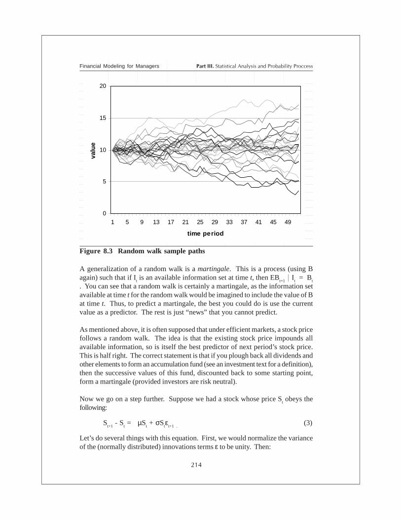
Part III. Statistical Analysis and Probability Proccess
214
Financial Modeling for Managers
0
5
10
15
20
1 5 9 13 17 21 25 29 33 37 41 45 49
time period
valu
e
Figure 8.3 Random walk sample paths
A generalization of a random walk is a martingale. This is a process (using Bagain) such that if I
t is an available information set at time t, then EB
t+1 * I
t = B
t
. You can see that a random walk is certainly a martingale, as the information setavailable at time t for the random walk would be imagined to include the value of Bat time t. Thus, to predict a martingale, the best you could do is use the currentvalue as a predictor. The rest is just “news” that you cannot predict.
As mentioned above, it is often supposed that under efficient markets, a stock pricefollows a random walk. The idea is that the existing stock price impounds allavailable information, so is itself the best predictor of next period’s stock price.This is half right. The correct statement is that if you plough back all dividends andother elements to form an accumulation fund (see an investment text for a definition),then the successive values of this fund, discounted back to some starting point,form a martingale (provided investors are risk neutral).
Now we go on a step further. Suppose we had a stock whose price St obeys the
following:
St+1
- St = µS
t + σS
tε
t+1 . (3)
Let’s do several things with this equation. First, we would normalize the varianceof the (normally distributed) innovations terms ε to be unity. Then:
215
Chapter Eight. Introduction to Stochastic Processes
(i) The left hand side is the change in the price of the stock.
(ii) The first term of the right hand side is known at time t, which we shall take hereas the current time. It says that there is a predictable component to the changein the stock price, which corresponds to a percentage growth µ. This term iscalled the drift term of the process.
(iii) The second term on the right hand side contains the news to transpire betweent and t + 1. We conventionally normalize the variance of the innovation itself(that of ε) to be unity. The term σ then becomes the instantaneous standarddeviation of the random component of the proportional change in S. It is alsocalled the volatility.
Equation (3) could be rewritten as an equation in the proportional change:
. S
S - S = SS where + =
S
S
t
t + t
t
tt
t
t 11 ,
∆∆+σεµ
If you divide both sides of (3) through by St as shown, then you can clearly see that
the drift parameter µ and the standard deviation parameter σ refer to theproportional changes. Now let’s take yet another step. We can think of a processB
t whose increments are equal to the given innovations process, ε
t. That is, ∆B
t =
Bt+1
- Bt = ε
t+1 is a sort of cumulated state of the world, the sum of all past news.
Then we can rewrite (3) as:
∆St = µS
t + σS
t∆B
t (4)
Finally, convert to continuous time by imagining that the time intervals for our discretetime t process get smaller and smaller, and infinitesimal. As Appendix A5 oncalculus shows, we imagine that the finite increments ∆S
t are replaced by the
infinitesimal increments dSt. In this case, (4) is written schematically in the form:
dSt = µS
t + σS
t dB
t (5)
The term µ is called the instantaneous drift of the process S, while the term σ iscalled the instantaneous volatility of the process. The process S
t is an example of
an Ito process.
Equation (5) can also be read as follows:
If we imagine the division of time into infinitesimally small intervals t, t + dt,then the conditional expectation of S at time t + dt, given information I
t available
at time t, is given schematically by:

Part III. Statistical Analysis and Probability Proccess
216
Financial Modeling for Managers
E ( St+dt
- St )* I
t = µS
t times the interval length dt
In other words:
. t d = S
Sd E
t
t µ)(
So µ is the instantaneous expected rate of increase in the stock price.
Along with an instantaneous mean, the stock price S at time t + dt will have aninstantaneous variance. In this case, things are constructed so that the varianceof the proportional change in S is equal to σ2 multiplied by the interval length dt.
You can use this property to estimate σ2. Suppose your unit of time is one day.Then the σ2 is simply the variance of daily proportional changes in the physical.Alternatively, if you assume the unit of time is one year, then σ2 is the annualvariance. Because these are variances of proportional changes, the correspondingstandard deviation σ comes out with the dimension of percentage. So if the timeperiod is annual, the σ is the standard deviation of annualized proportional changes.See Example 8.2 below.
Finally, both µ and σ can depend on time, and even on the value St. For example,
we could specify:
µt = k ( S* - S
t ) ,
where S* is some constant value and k is a constant representing a speed ofadjustment. This sort of formulation is called an error adjustment mechanism. Itsays that there is some target level of the stock price S*, and the stock price can beexpected to drift upwards if the current value is less than the target, or downwardif the current value is greater than the target. In addition, the second term on theright hand side is the unforeseeable random volatility component, which is essentiallyunpredictable.
Example of an Ito process
Suppose a stock that pays no dividend has a volatility of 29% per annumand an expected return of 12% per annum (by convention, we assumecontinuous compounding). We shall operate with the year as the unit oftime. So we can set µ= 0.12 and σ = 0.29. The Ito process for the stockprice is:
Example 8.2
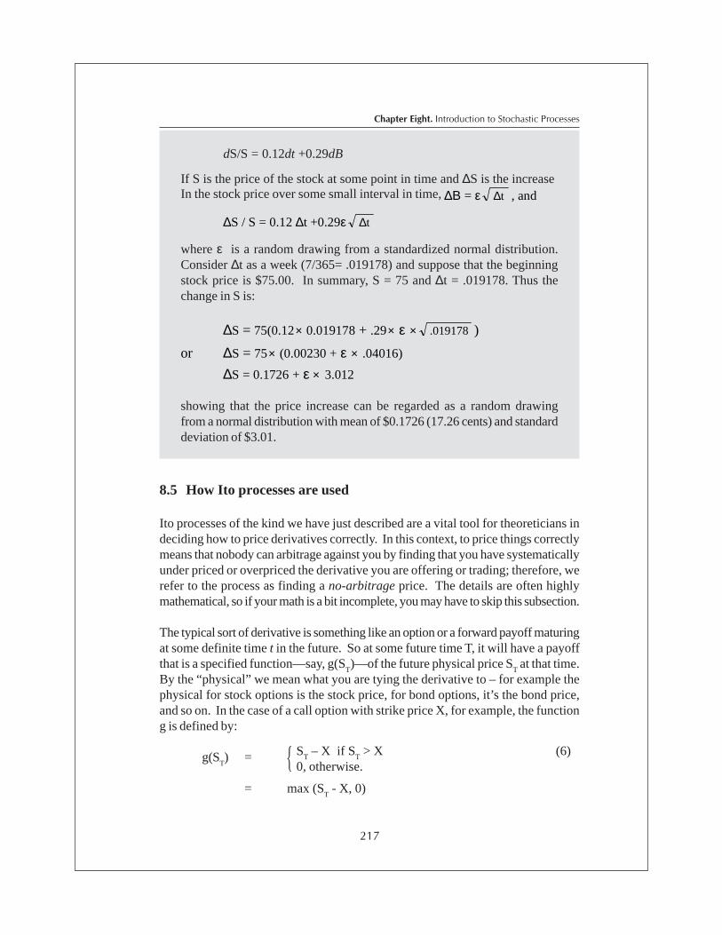
217
Chapter Eight. Introduction to Stochastic Processes
8.5 How Ito processes are used
Ito processes of the kind we have just described are a vital tool for theoreticians indeciding how to price derivatives correctly. In this context, to price things correctlymeans that nobody can arbitrage against you by finding that you have systematicallyunder priced or overpriced the derivative you are offering or trading; therefore, werefer to the process as finding a no-arbitrage price. The details are often highlymathematical, so if your math is a bit incomplete, you may have to skip this subsection.
The typical sort of derivative is something like an option or a forward payoff maturingat some definite time t in the future. So at some future time T, it will have a payoffthat is a specified function—say, g(S
T)—of the future physical price S
T at that time.
By the “physical” we mean what you are tying the derivative to – for example thephysical for stock options is the stock price, for bond options, it’s the bond price,and so on. In the case of a call option with strike price X, for example, the functiong is defined by:
g(ST) = 9
= max (ST - X, 0)
dS/S = 0.12dt +0.29dB
If S is the price of the stock at some point in time and ∆S is the increaseIn the stock price over some small interval in time, ∆Β = ε t ∆ , and
∆S / S = 0.12 ∆t +0.29ε t ∆
where ε is a random drawing from a standardized normal distribution.Consider ∆t as a week (7/365= .019178) and suppose that the beginningstock price is $75.00. In summary, S = 75 and ∆t = .019178. Thus thechange in S is:
∆S = 75(0.12× 0.019178 + .29× ε × .019178 )
or ∆S = 75× (0.00230 + ε × .04016)
∆S = 0.1726 + ε × 3.012
showing that the price increase can be regarded as a random drawingfrom a normal distribution with mean of $0.1726 (17.26 cents) and standarddeviation of $3.01.
ST – X if S
T > X (6)
0, otherwise.

Part III. Statistical Analysis and Probability Proccess
218
Financial Modeling for Managers
The payoff is a promise to pay a formula amount that is contingent upon whateverthe final physical price turns out to be. At time t < T, such a promise will have amarket value, and the trick is to find out just what it ought to be.
At first sight, this might appear to be like deciding how long is a bit of string – thepromise could be worth anything, depending upon what people are willing to payfor it, who is in the market, and so forth. However, there is a unique correct price.The reason is that the derivative provides no new information. It is purely a piggybackinstrument. Since it provides no new information, you ought to be able to replicateall its price movements in the interim through to time T, by means of a position inthe underlying physical, plus a risk-free asset such as a call account (often bondsare considered an example of this, but we know by now that bonds are hardly risk-free!). It is this principle that enables us to derive the equation that the derivativeprice should satisfy, and, by solving that equation, the theoretical formula for theprice of the derivative as well.
Suppose that the current price of the option is some unknown function C of thecurrent stock price S and time t.
Yt = C ( S
t , t ). t<T (7)
According to a result called Ito’s lemma, you can say that Yt must itself obey an Ito
process, and you can specify what the mean (i.e. the drift term) of this processmust be in terms of the partial derivatives of the function C. (See Appendix A5 fora discussion of partial derivatives.)
Then you construct a replicating portfolio in terms of some – as yet to be determined– portfolio amounts a
t, b
t , so that:
Yt = a
t S
t + b
t A
t , (8)
where At is the price of the call account, a notional construct in which you assume
that $1 has been invested at t = 0, and allowed to accumulate at the risk free rateuntil the chosen time t. In other words, with continuous time accumulation as inchapter 2.4, A is equal to ert, where r is the risk-free rate.
By matching up the amounts at, b
t in (8) with the drift term in the Ito process for Y
t
as derived from (7), you can write down a partial differential equation that theunknown function C must satisfy. Then you add the terminal or boundary condition(6), and—presto!—out comes the theoretical price of the option. It turns out thatthis price depends on a number of factors: the current stock price S
t , the volatility
σ of the S process, the interest rate r, the strike price X, and the time t, via the timeto maturity.

219
Chapter Eight. Introduction to Stochastic Processes
The Black-Scholes formula
The Black-Scholes model derives the following equation for the price c of a calloption:
c = SN(d1) - Xe-rT N(d
2 ) (9)
where: N(d) is the value of the Normal distribution function at the point d; d = d1 or
d2. The other symbols are defined as follows:
S = current price of the underlying physical
X = strike price of the option
T = time to maturity
r = current risk-free interest rate
; T
T/ + r + S/X =d
σσ )()ln(
22
1 (9a)
;)()ln(
T - d = T
T/2 - r + S/X =d 1
22 σ
σσ
(9b)
σ = volatility of the physical
You will notice in this formula that the price does not depend upon the mean µ. Ineveryday language, investor expectations are irrelevant to the price of the option.This may seem like a startling statement. However, it is simply a reflection of thefact that investor expectations do play a role, but only in the price of the underlyingphysical. The option itself is purely a play on the physical, and the effects ofchanging expectations can be hedged away by means of the corresponding effecton the physical (the latter being the hedge).
However, this hedging process does not apply to the volatility σ, which appearsunavoidably in the price of the option. You can see intuitively why this must betrue. Compare two call options, one with a high volatility and the other with low.Suppose that the option is a call option, which is currently a bit out of the money. Inother words, the current physical price is slightly less than the strike price of theoption, so you would get nothing if you decided to cash in your chip at this point in
Part III. Statistical Analysis and Probability Proccess
220
Financial Modeling for Managers
time. Of course you wouldn’t decide to cash in now anyway, because though yourchip is out of the money right now, it could well be in the money at some time in thefuture. It is definitely worth something because of that possibility; hence, the optionprice is by no means zero. The option with a higher volatility has more chance ofgetting back in the money next period than does the one with the lower volatility, soit makes sense that it is worth more.
Nevertheless, you do have to be able to form an estimate of the physical’s volatility,and we shall discuss this below. In the meantime, we note that if we knew whatthe option was currently trading for, then we could use an equation such as (9) toreverse the process and solve for the implied volatility in terms of the current priceof the option. This process is called backing out the implied volatility.
These days, theoreticians use a somewhat simpler approach, which is based onconverting the underlying process S
t into a different world where everybody is risk
neutral. In such a world, all assets would have exactly the same expected return;this would be the same as the risk-free rate r. Here, you can price the derivative assimply the mathematical expectation of the discounted value – at rate r – of itsterminal payoff. To compute that expectation, you use the transformed Ito process—that is, the version that would hold in a risk free world. There are rules that enableyou to obtain the modified Ito process, which is called an equivalent martingaleprocess.
In practical terms, even the equations for the derivative price are usually ratherdifficult to solve. The Black Scholes was an exception, though even this eludedresearchers for years. As a general procedure for other kinds of derivatives, orother specifications for the driving physical price processes, solving for the optionsprice is often done numerically. This may be achieved by means of a number ofapproaches. One is to approximate the Ito process in terms of a simpler Binomialprocess. In this approach, the possible variation in S over a very short time periodfrom t to t + ∆t is constrained to just two possibilities: up a certain fixed magnitude,or down a certain fixed magnitude. It turns out that you can approximate an Itoprocess quite well by this method. Arriving at a solution can then be done bymeans of discrete programming techniques.
From a trading point of view, everything changes once you have a technique for thetheoretically correct price. The only unknown parameter in the option price is nowthe volatility, σ. So deciding what it ought to be is essentially a guessing game.First, one can get a handle on it from the historical record of the variance in thephysical prices—we’ll look at this in the next section. But on top of that, there isalways margin for decision as to what the correct volatility for the coming periodought to be. So trading takes place on the basis of just such a guessing game; in

221
Chapter Eight. Introduction to Stochastic Processes
finance terminology, we say the options market tends to trade on volatility. Playerswho write options have to think not only about hedging the dependence of theoption price as the underlying physical price changes (delta hedging), but also hedgingas the volatility is judged to be changing (vega or kappa hedging). Those who tryto make money out of options as an uncovered position will do it on the basis ofwhat they think are superior insights as to the s in the coming period – (these aresometimes called vega plays and the practitioners vegamites). The term for theactivities we’ve been describing is volatility trading.
Backing out implied volatility using Goal Seek
In this example we shall first calculate the Black Scholes option price for acall option on the S&P500 Index. Then we shall assume a different thoughtexperiment in which the option price is set at a certain magnitude and wefind out what the implied volatility must be. To do this, we shall use a veryuseful Excel capability called Goal Seek, which operates by adjusting oneof the cells to achieve the result that you want from a given formula.
Here is your base data, and cells we suggest you enter them into:
(So this call option is just a bit out of the money, with no immediate exercisevalue.) You can enter suitable names for the above data in column A, suchas “Current SPI” in [A3], and so on. The unit of time will be annual. Thematurity in annual terms will be T = C8/365 = 60/365. You can take theinstantaneous risk free rate r to be simply [C5] = 0.055.
Task 1: Calculating the Black Scholes price
Set aside cells [C11] and [C12] for d1 and d2 respectively. You will useFormulas (9a) and (9b) to compute them. For the spot or current price S,we do not use the current SPI value as it appears in [C3], because the
Example 8.3
Data Item Value Cell address
Current SPI value 1234 C3 Annual Volatility 0.20 C4 60-day CD rate (annualized) 0.055 C5 S&P500 Divided yield 0.018 C6 Desired Maturity for option (in days) 60 C8 Strike price of option 1250 C9

Part III. Statistical Analysis and Probability Proccess
222
Financial Modeling for Managers
Black Scholes call option price changes a bit when the stock pays a dividend.You don’t get the dividend until you have actually called the stock, so in themeantime the lack of dividend entitlement means that you have to discountthe current stock price (here the SPI), which does carry a dividendentitlement, by the dividend yield. The simplest way of handling this is tocalculate the value of S as an intermediate value in, say, cell [D10] as:
= C3*EXP(-C6*C8/365)
and then refer to [D10] when you enter Formula (9a). Note that we areusing continuous time discounting here.
When you enter the two formulas for d1 and d2, it is always useful to enterthe cell addresses for the input parameters rather than the values themselves.You will find the formula gets rather long for d1 in particular and youwould have to concentrate pretty hard! To make the whole process easierfor yourself, break the formula up into intermediate calculations, placingthem in cells to the right of the main calculation, as we did above for thevalue of S. Watch that left hand and right hand brackets match in number,and are entered in the right places.
When you have finished entering, the results should be d1 = - 0.04332 incell [C11], and d2 = - 0.12441 in cell [C12].
Next, enter the call price as calculated from Formula (9) in cell [C14]. Youwill have to use normsdist() function from the Function Wizard (look inStatistical), and in the brackets put the cell references [C11] for d1, and[C12] for d2. Your final result should come out to $35.87 as the call optionvalue.
Task 2: Backing out an implied volatility
Now suppose a dealer quoted us an option price of just $35.00. Whatcould you say about the value of the volatility the dealer was using, assumingthat she is also using the Black Scholes formula, but is not using yourpatented volatility estimation technique?
Cell [C14] is the crux of your operation, which brings everything together.Now suppose we put the result of this cell as 35.00, which means that theentry in cell [C4] must be changed. You can try fiddling around on this, butit will take you quite some time to come up with exactly $35.00 as theoutcome.

223
Chapter Eight. Introduction to Stochastic Processes
8.6 Volatility models
The previous section referred to the importance of volatility estimation. The naturalstarting point is the historical record, even if the trader will subsequently adjust hisestimate upwards and downwards by assessing the conditions likely to arise overthe coming pricing interval.
A naive estimate of historical volatility is simply the variance of the historical series.A common device is to recognize that volatility can change, but hopefully onlyslowly, so you adopt a moving sample. Thus, if the series record is monthly overthe past 20 years, you could adopt a three-year frame, which would give you 36observations, and move this along by one month at a time, so that the most recentestimate would be based only on the last 36 months. There are lots of variations onthis sort of approach.
A better approach is to combine modeling the conditional mean of the physical Sand the conditional variance. In doing so, we recognize explicitly that the volatilitythat we need is what will transpire over the coming period, and this is alwaysconditional on the latest information that we have.
To follow this approach, we specify a regression equation. Schematically:2
St = µ ( past S, other available variables ; β ) + ε
t (10a)
plus a volatility equation: if Var ( εt ) = σ
t2 ,
σt = f ( past σ , ε
t ) (10b)
Goal Seek does the job automatically. Go into Tools/Goal Seek, and threeoptions which require entries will pop up. You wish to set cell [C14] tovalue 35.00 by changing cell [C4]. Once you’ve done this, the result isproduced: an annual volatility of 0.1956, or 19.56% appearing in cell [C4].This makes sense—because the dealer is quoting a lower price, all elsebeing the same, she must be using a lower volatility.
Don’t delete your spreadsheet just yet. You can use it to do problem 5 atthe end of the chapter.
2 Note that in what follows the innovation εt now has variance σ2, rather than unity.

Part III. Statistical Analysis and Probability Proccess
224
Financial Modeling for Managers
Equation (10a) is called the mean equation, and in this context µ is the conditionalmean of S
t (rather than ∆S
t ). The symbol µ (....) is just a way of saying that the
conditional mean µ is thought to depend upon a string of variables that are listedinside the brackets, but that we have yet to specify the exact functional nature ofthe dependence. It says that the physical price is explained in terms of the conditionalmean µ (which is some function specified by the researcher of past informationand any other available variables.) For instance, if you have monthly data, themean could depend upon dummy or categorical variables to represent the particularmonth effect. For the definition of seasonal dummies, see an econometrics text.
Equation (10b) is the variance equation, presented with the same generalized notationexplained above in connection with the mean. It specifies how the volatility is toevolve. You will notice something about this equation. It is not specified in termsof things that can be directly observed. To get the σ and ε’s to put into (10b), youhave to estimate them from (10a). More precisely, (10a) and (10b) must be estimatedjointly, and this can certainly be done.
Different approaches specify the functions µ (.) and f (.) in different ways. Apopular approach is based on the ARCH family, or Auto Regressive ConditionalHeteroscedascity. (You can see why the acronym is used!) Since its originaldevelopment by Robert Engle in 19823, various sons and daughters have beendeveloped (GARCH. MGARCH, IGARCH – AAAARGH!), none of which wewill bother explaining here. A typical ARCH specification in finance would be:
St = β
0 + β
1S
t-1 + β
2x
t + β
3σ
t + ε
t (11a)
σ t2 = α
0 + α
1ε
t-12 (11b)
The first equation is the mean equation, since the first four right hand variablesare intended to capture the conditional mean µ
t. The variables x
t represent any
exogenous variables you think might be important. The variable σt is the current
volatility, which suggests that it might affect the mean (because it feeds back intothe pricing of assets).
The second equation is the volatility equation. It says that the residual from themean equation has a variance that depends upon the latest squared residual availableup to time t. The idea is that if the system gets shocked off the mean path in thelast period (a big forecasting error ε
t-1), then system volatility should go up. In
acronym, version (11) is called a MGARCH ( mean generalized ....)
3 Engle, R.F. (1982) “Autoregressive conditional heterscedascity with estimates of the variance of United Kingdom Inflation.”Econometrica, 50, 987-1007.

225
Chapter Eight. Introduction to Stochastic Processes
Equations 11(a) and 11(b) can be estimated by a technique called maximumlikelihood (ML), which is often used in statistics and econometrics. Essentially itestimates all the parameters (here the betas and alphas) by choosing them to maximizethe probability of getting the data series S
1, S
2 .... S
N actually observed. The ML
technique is necessary here because the volatility terms σt in Equations 11(a) and
11(b) are not observable, and the technique in effect imputes these at each roundof the numerical likelihood maximization, which is based on iterating values of thealpha and beta parameters at each step.
The ML technique can be quite tricky to implement, since it relies upon numericalalgorithms that may not converge. Also, sometimes the ARCH model simply doesnot fit. There are alternative specifications to the ARCH family. One of these isdue to Schwert4, which estimates the current volatility based on the absolute valueof the residuals to the fitted mean equation, and uses more or less straightforwardregression techniques to execute the necessary steps. For an application to foreignexchange, see Bowden and O’Donovan (1997)5, which also describes the technique.
It is important to note that in real life trading, ARCH, Schwert, and other volatilityestimation techniques are only the first step. The objective is to begin by estimatingthe current volatility on this somewhat mechanistic level, and then to look at theresult and adjust it according to your own perceptions of the state of the world. Forinstance, if a Vogon spaceship suddenly appears at the Athens Olympics openingceremony, it might be worth revising your computed σ upwards (on the off-chancethat it is not a publicity stunt).
At any rate, you arrive at a conclusion as to what the volatility should be. Then youlook at how the options for the preferred month – or all the months, for that matter– are priced in the market. You can then back out the implied options price andcompare this with your own view of what the volatility is likely to be. Maybe youhave private knowledge from your Sub-Etha Sens-O-Matic of the likely arrival ofthe aforementioned spaceship. If you think that the market is underestimating thevolatility, you can try a bit of volatility trading. Of course, options have many uses,not least of which is hedging portfolios, where they represent a convenient way ofprotecting the portfolio manager against downside risk in the fund’s portfolio ofshares or bonds.
5 Bowden, R.J. and B. O’Donovan (1996). “Financial markets: volatility and policy.” In B. Silverstone, A. Bollard & R.
Lattimore (eds) A Study of Economic Reform : The Case of New Zealand, pp 279-314. Amsterdam: North Holland.
4 Schwert, G.W. (1989) “Why does stock market volatility change over time?” Journal of Finance, 44, 1115-53.

Part III. Statistical Analysis and Probability Proccess
226
Financial Modeling for Managers
8.7 Other time series buzzwords
In many cases, the physical price series St is likely to be non-stationary, which
means that its variance and other characteristics are likely to change over time.Actually we have to be a little careful here. By the variance, we mean theunconditional variance, which is what you might compute if you took the samplevariance of a very large number of observations, ignoring the temporal structure,and treated them as some sort of random sample. This has to be distinguishedfrom the conditional variance, which is the variance of S
t+1 given S
t and any other
information available at time t. The conditional form may be thought of as theincremental variance, and the unconditional type as the total system variance.
Indeed, one important form of non-stationarity is where the stationary distribution,and hence the total system variance in the sense defined above, simply do not exist.We have already seen an example of this in the random walk, where the varianceexploded over time, even though the conditional variance, which was the varianceof the random increments ε, remained the same for all time. Lots of empiricalprocesses behave this way, even if they do not have exactly the form of the randomwalk. Examples include stock prices, foreign exchange rates, and sometimes stockmarket returns. Such processes are said to have a unit root. The precise referencewill not concern us too much here, but basically refers to the difference equationobeyed by the process, which would specify the way that S
t is derived in terms of
St-1
and past S values. There is a certain polynomial equation associated with thisdifference equation, and you can solve for its roots: if they are equal to or greaterthan one, then you know the whole process will explode over time, something likeFigure 8.3 above.
Processes that explode in this way are often called integrated processes. To seewhy, recall the random walk. By a process of backward substitution, this can bewritten:
Bt
= εt + B
t-1
= εt + ε
t-1 + B
t-2
= εt + ε
t-1 + ε
t-2 + . . . . forever
The word “integrated” means summed, and you can see why this might be appliedto the random walk. It can be viewed as the progressive outcome of all the summedpast values of the innovations terms (recall these are the ε’s). In stationary processes,the influence of the innovations in the distant past dies away. For instance, considerthe process defined by:

227
Chapter Eight. Introduction to Stochastic Processes
yt
= λyt-1
+ εt
= εt + λε
t-1 + λ2 y
t-1 . . . . .
= εt + λε
t-1 + λ2 ε
t-2 + λ3 ε
t-3 + . . . . . forever
The second equation is obtained from the first by a process of backward substitution.If the parameter λ is less than one in absolute value, you can see that the influenceof ε
t-100 (i.e. the news 100 periods ago) is hit by a coefficient λ100, which is very
small. Compare this to the random walk where the coefficient of εt-100
remains atone, just the same as the coefficient of ε
t. So whether *λ*< 1 or *λ*$ 1 makes a
great deal of difference. In the former, you can show that the unconditional varianceVar (S
t) exists, but in the latter it does not exist – only the conditional variance Var
(εt) = σ2.
Suppose that we take the first differences of the random walk. We get:
Bt - B
t-1= ε
t
So the differenced random walk is just the innovations process. This is perfectlystationary; certainly the variance of ε
t exists, and in fact it is the same as Var
(εt-1
) and so forth. We would say that the original Bt is I(1), which is a shorthand
way of saying that it is integrated of order 1, which, in turn, is a way of saying thatif you difference it just once you will get down to a stationary process (denoted I(0)). Sometimes processes are so badly non-stationary that you have to differencethe difference to get down to a stationary process – these would be I(2) or worse.Most financial processes are I(1) or I(0).
Cointegrated processes
The above ideas extend to vector processes, in which we deal with two or moreprocesses at a time, so that each can be regarded as an element of a vector. Forinstance, we could look at a vector process whose first element is the price of aspecific stock, the second element is the price of the market, and the third is thevalue of the risk-free rate.
Often all the elements of a vector process are non-stationary, but there is anequilibrium relationship between them, which is itself stationary. For example, wesaw in Chapter 7.5 that the CAPM specified that the return on a stock (number i,for instance) is related to the market return R
t and the risk-free rate ρ
t by:

Part III. Statistical Analysis and Probability Proccess
228
Financial Modeling for Managers
ri,t
= ρt + β
i (R
t - ρ
t ) + ε
i,t
Now it might be that ri,t is non-stationary, and so are R
t and ρ
t. But the disturbance
process εi,t is stationary. This is perfectly possible. It means that although the
return on the stock, the market return, and the risk-free rate can drift all over theplace, there is a kind of flexible rope always holding them together, so that therelationship is shocked (the ε terms) but only in a stationary way. In this case, thethree variables r
i,t, R
t and ρ
t are said to be co-integrated.
Where series are co-integrated, it turns out that you can always write a version ofthe relationship in which the change in one variable can be represented as the sumof the past changes in itself and the others, plus a term which represents the extentto which the equilibrium relationship was departed from in the past periods. This isthe error correction representation; the error is in the equilibrium relationship,and the idea is that the variables adjust over time to remove these errors and keepit within coo-ee of the equilibrium relationship.
Detailed study of these relationships is a little outside the scope of this book. Ingeneral, the purpose and value of time series models and methods is that theyenable us to get a handle on the disturbance elements – the ε ‘s. It is the latter –or, more specifically, their variances – that are so useful for pricing derivatives.The relationships are also useful in themselves for forecasting, in situations whereyou are after an uncovered gamble. In this type of scenario, it is the conditionalmean – the µ function – that now occupies center stage. It gives you the expectedvalue of the stock price (or whatever physical you are interested in) as a functionof the information available to you. When you model the conditional mean, you arein effect forming your own forecasting mechanism. The residual variance fromthis equation will give you some idea of the extent to which your forecast is likely tobe wrong. In statistical jargon, the conditional variance can enable you to formconfidence bands for your forecast. You would present the latter in the form of thepoint forecast – which is your computed value of the conditional mean – plus orminus one sigma for instance, which is the estimated standard deviation of theresidual variance in your fitted relationship.
At this point, we draw a curtain on the discussion of stochastic processes and theirapplications. You already have a sense that this is an enormous topic, and an areaof active research and applications programs both in academia and in industry. Ithas many important applications like derivatives pricing, forecasting, and riskmanagement.

229
Exercises
81. Can you think of some more examples - and perhaps better ones! – where you
might want to hedge some price or return, but the available derivative instrumentis not perfectly correlated with your target?
2. It has been said that the CAPM model and related portfolio models representa form of hedge relationship. Suppose that you are a portfolio manager, andyou find a stock that has a negative beta on the market.
(i) What does this mean about its expected return over the coming periods,relative to the risk-free rate?
(ii) Can you rationalize this in terms of the value of such a stock in terms ofany specified hedging need?
Suppose, for instance, that the stock is an undertaking firm that specializes inexpensive interments for highly strung stockbrokers. Would such a stock havea special value in your portfolio, and why?
3. (You may need a bit of help with this one.) Take a random walk process asspecified in the form (2) of Section 8.4 in the text. You are now at time 0, andyou know B
0.
(i) What is the predicted value of B1? What is the variance of the prediction,
that is, the variance of the discrepancy between your predicted value andthe actual outcome?
(ii) Do the same for B2 at time 2. Predict the value knowing only B
0 at time 0,
so you have to form the best predictor available and then find its variance,conditional on the information available at time 0.
(iii) Carry it on until some time T in the future. How does the predictive varianceaccumulate as the horizon T gets larger and larger?
4. Repeat Question 3 but this time with the process:
yt = λy
t-1 + ε
t
Analyze the way in which the variance of your forecast increases or decreaseswith the horizon T, and relate this to the size of the absolute value of the parameterλ .

230
Exe
rcis
es 8
5. Use your data in Example 8.4 to explore the time value of the option. Graphthe price of the SPI call option against maturity. Notice how the time valuediminishes more rapidly, the closer you get to option maturity. (In hedging theirportfolios, fund managers sometimes buy options on the SPI when they areworried about some forthcoming event, relying on keeping options costs down by selling the option in the near future before the time value starts decaying onthem.)

231

232

Part FourMANY VARIABLES
233

234

NineNineNineNineNineMany Variables
235
Sometimes in finance, one has to handle situations where there are many variablesto study or to control in some way. An obvious instance is in portfolio theory. Inthis context, having many stocks in your portfolio is regarded as good practice, as itenables you to diversify risk. But it does mean that one has to be able to manipulatenot just one or two portfolio proportions, but a whole set of proportions. You canplay around with the resulting decision problem by using elementary algebra, butthe results can be atrocious and will almost certainly lead to error because thingsget messy pretty quickly. The methods of matrix algebra are a very natural way tohandle this sort of situation. They can also help you remember results and propertiesa lot easier than you could otherwise! In this chapter we shall first give an abridgedaccount of the basics of vectors and matrices, and then indicate the sort of situationswhere they can help. In particular, we will look into the formation of portfoliosusing mean—variance analysis.

Part IV. Many Variables
236
Financial Modeling for Managers
9.1 Vectors and matrices
A vector is a one-dimensional array of numbers, usually written in the form of acolumn vector, which is a set of numbers placed one on top of the other. The arrayis given a name, and the name is usually written in bold type, as distinct from thenames of ordinary variables, or scalars in this terminology, which are written inordinary type. For example, we might have the vector:
x = .
5
3
2
Vector x is a 3 x 1 vector of numbers. We could denote the representative elementof the vector x as x
i , with the index i running from i = 1 to i = 3:
x =
x
x
x
,
3
2
1
where in this case, x1 = 2, x
2 = 3, x
3 = 5.
A matrix is a rectangular array of numbers. For example,
. = A
243
501
112
Here the matrix A (we use uppercase but not bold) has order 3 x 3, meaning that ithas three rows and three columns. This particular matrix is square; it has an equalnumber of rows and columns. The representative element of a matrix A is writtena
ij, meaning the element in the ith row and the jth column.
Notice that we could regard the above matrix as being made up of three vectors,each of order 3x1, placed side by side:

237
Chapter Nine. Many Variables
A = [ a1 , a2 , a3 ]
where: a1 =
3
1
2
a2 =
4
0
1
a3 =
.
2
5
1
Actually, to qualify as a matrix, it is not enough to be just a rectangular array ofnumbers. The array also has to obey certain operational laws, which stem from itsmathematical background in coordinate geometry as the representation of a linearoperator. For our purposes, the most important of these rules concerns multiplication.
Suppose you have a vector like x above. Then the product Ax has the followingmeaning: it is a vector whose elements are obtained by means of the schemedepicted below.
9
6. xa + xa + xa = with =
x
x
x
aaa
aaa
aaa
323222121
3
2
1
333231
232221
131211
??
???
??
?
In this scheme, to get the second element of the product Ax, we go across thesecond row of A and multiply each element of that row with a succeeding elementof the vector x, adding the results. We do the same for the first and third elementsof the product. Now try this out by taking the product y = Ax, where x and A arethe earlier numerical examples. Verify that:

Part IV. Many Variables
238
Financial Modeling for Managers
y = .
28
27
12
You will see that this process will only work if the number of columns of A is equalto the number of elements (rows, in this case) of the vector x. In this case, A andx are said to be conformable.
Example: The vector of ones, or summation vector, is particularly useful:
1 =
1
1
1
Can you verify that the vector A1 is equal to the sum of the columns of A?
Now suppose that we have another matrix X, with columns x1 , x
2 , x
3 , x
4 . Each
of the columns can be treated as a column vector itself. So we can attach ameaning to the product Z = AX. Each column z of the matrix Z will be obtained asthe product of A times the corresponding column of the matrix X, the latter treatedas a matrix - vector product, in the manner just outlined. In other words,
Z = AX = [ Ax1 , Ax2, Ax3, Ax4 ]
Again, this will only work if the number of columns of A is equal to the number ofrows of X, in which case, A and X are conformable. If this is the case, we canbuild up the product of two matrices by taking the first times each column of thesecond in turn, and putting them side-by-side. The order of the resulting product isequal to the number of rows of A by the number of columns of X. A good mnemonicis to write the orders of AX as [3 x 3] x [3 x 4]. The two inner numbers have to bethe same for conformability, and the two outer numbers give the order of the result,as [3 x 4].
You will notice that you have to be a bit careful about the order in which you writethe product. Thus XA means something quite different from AX. Indeed, even ifthe first product does exist, it does not follow that the second product exists - theconformability requirements are quite different.
In Question 1 at the end of this chapter we have given several matrix multiplicationproblems, using easy numbers. If you are not already conversant with matrixproducts, you should work through these before proceeding.

239
Chapter Nine. Many Variables
The transpose of a matrix A, written A', is the matrix constructed by turning therows of A into columns. For example:
. = A then = A
′
251
401
312
243
501
112
A square matrix, A is symmetric if ai,j = a
j,i. In other words, if you interchanged
rows and columns, the new matrix would be just the same as the old one. You willnotice that if A happens to be symmetric, then A = A'. Of course, A can only besymmetric if it is square to begin with.
You can have the transpose of a vector, too. In this case, a single column becomesa single row, often called a row vector.
x =
5
3
2
x' = [ 2 3 5 ]
Now suppose we take the matrix, A, which is symmetric:
. = A
241
401
112
(Check that A is symmetric, in terms of the definition given above.)
Now we form the following triple product:
q = x' A x.
Let us check that we can do this properly to begin with, that is, that everything isconformable. Take the last product, Ax. A has 3 columns and x has three rows,so the product will exist, and be of order 3 x 1, the number of rows of A by the

Part IV. Many Variables
240
Financial Modeling for Managers
number of columns of x (which, incidentally, is one, since it is a vector). The resultis a vector of order 3 x 1. The transpose x' is a row vector of order 1 x 3. The laststep is to multiply a row vector by column vector: 1× 3 by 3 × 1, and you can seethat the result exists and is of order 1 x 1. This means that it is just a single number,or a scalar. Go ahead and try it. You will find that the result is:
q = 2x12 + 2x1x2 + 2x1x3 + 8x2x3 + 2x3
2
Could you have guessed what the coefficients of this expression are, just by lookingat the matrix A?
This sort of expression is called a quadratic form. Every term in it is of powertwo: either a square like x
12 or a product like x
1x
2. Conversely, every quadratic
form can always be represented as x' A x, for some symmetric matrix A.
9.2 Matrix inverses and equation solving
Suppose we have an equation
3x = 6
We assume you are able to solve this, hopefully without much difficulty. We couldwrite the solution in the form:
x = 3-1 6
where you will recall that 3-1 is just another way of writing 1/3. The answer, ofcourse, is x = 2.
Now we are going to do the same sort of thing for solving systems of equations,which are linear simultaneous equations such as :
3x1 + 2x
2 = 4
x1 + 5x
2 = 1
You may know how to work out the solutions for x1 and x
2 already. It's easy for
this 2×2 set of equations and variables, but you'll need something more than highschool algebra when it comes to solving 14 × 14 problems!
Before we can move on, there is a little more work to do on matrices. One specialmatrix will be important: the identity matrix, denoted I. This is a matrix with ones
241
Chapter Nine. Many Variables
all the way down the leading diagonal—which is the diagonal leading from top leftto bottom right—and zeros in all the off diagonal positions. For example the 2 x 2identity matrix is:
. = I
10
01
Write down the 3x3 identity matrix.
The identity matrix plays the role of the number one (1) in matrix work. If you takeany conformable matrix and multiply it by I, you get the same matrix you startedwith; thus I A = A or A I = A. Similarly, if x is a vector, I x = x . (Would x Imake sense?) Now take a matrix A. It has to be square. Under suitablecircumstances—more on this later—we can find another matrix, denoted A-1 ,such that:
A-1 A = I
If we can find such a matrix, it is said to be the inverse of A. For us to be able tofind such a matrix, we need the matrix A to be of full rank. By this we mean thatthe columns of A must be genuinely different. For example, consider the matrix:
, = A
843
001
212
or the matrix
. = B
273
5111
142
You can see why matrix A might have a problem. The third column of A is justtwice the second, so in a sense the columns are not really different. The case B isa bit harder, but you might be able to see that the second column is equal to the firstplus twice the third. So once again, the columns are not genuinely different, sinceone of them can be manufactured out of the others. This property is called lineardependence. To be able to compute its inverse, we must have all the columns of

Part IV. Many Variables
242
Financial Modeling for Managers
A as linearly independent, meaning that you cannot get one from the others bysimply taking some linear combination of them. Such a matrix is said to be of fullrank or non-singular. In practice, the computer will tell you when the matrix youare trying to invert is singular, so you don't have to bother. The computer will alsodo the inverting, that is, finding A-1.
Now we move on to the use of matrix inverses. Suppose we have the following setof three simultaneous equations with three unknowns x
1 , x
2 , x
3:
2x1 + x
2 + x
3 = 2
x1 + 5x
3 = 3
3x1 + 4x
2 + 2x
3 = 5
Using your newfound skills in writing things in matrix-vector form, verify that theabove can be written as:
A x = b , (1)
where x =
x
x
x
3
2
1
b =
5
3
2
and. = A
243
501
112
You can see that all this is quite general. Any set of linear equations can always bewritten in the form (1).
Now multiply both sides of Equation (1) by the inverse A-1. (We don't mean to

243
Chapter Nine. Many Variables
calculate A-1 numerically; this is just matrix algebra we are doing here). Moreprecisely, multiply everything on the left hand side, or pre-multiply by A. SinceA-1A = I, the identity matrix, we get:
x = A-1 b
In effect, this has solved the system, just as x = 3-1 6 solved the simple one-variableequation. The computer can work out A-1 and multiply the given right hand sidevector by the inverse, and—Bingo!—there it is: the solutions for x
1, x
2, x
3.
Actually, the inverse of the matrix A is:
−
−−
−−− =A
154
9113
5220
23
11
Can you check that A'A = I? Now find the solution for x. We will not worry hereabout the algorithms used to calculate the inverse. Basic versions can be found inevery textbook of linear or matrix algebra.
9.3 Statistics with matrices
A lot of useful financial econometrics is concerned with the mutual relationshipsbetween many variables, such as a set of securities. Suppose that x
1, x
2,..... x
n is
a set of n random variables. Note that n does not mean the sample size here - it isthe number of random variables. For instance, in the data you have n = 14 individualstocks. We can combine the random variables into a random vector x which willbe of order n:
x = .
x
.
.
x
x
n
2
1
The vector random variable x will have a mean µµµµµ:

Part IV. Many Variables
244
Financial Modeling for Managers
E x =
Moreover, there will be variances and covariances between the various randomvariables. For instance, σ
12 = E (x
1 - µ
1 )2, or σ
12 = E (x
1 - µ
1)( x
2 -µ
2 ). We
can assemble all the variances and covariances into a matrix:
Σ =
⋅⋅⋅⋅⋅
⋅⋅⋅⋅
21
22212
11221
nn
n
n
σσ
σσσσσσ
Strictly speaking, we should write the (2,1)th element as σ21
and not σ12
, but theyare equal so we just use one and not both. A similar convention applies to all theother off-diagonal elements. We also use σ
12 instead of σ
11 (etc.) for the diagonal
elements.
Note that the Σ symbol does not represent the summation sign in this context. It issimply the uppercase * (for matrices, remember) version of the lower case σ
ij
inside. You will notice that it is a symmetric matrix, simply from the way it isconstructed.
Often the random vector x is specified to have a given probability distribution. Anexample is multivariate Normal. This has a similar shape to the unidimensionalNormal, but now has to be plotted in higher dimensions. For example, if you hadnormal density for two random variables, this would look like a bell in 3-D. Wewould say that x has the multivariate N (µµµµµ, Σ) distribution function or density.
Another way of writing the covariance matrix Σ is as follows:
Σ = E ( x - µµµµµ) ( x - µµµµµ )'
You can try writing this out in full by multiplying (x - µµµµµ) by (x - µµµµµ)', and then taking
. =
.
. =
x E
.
.
x E
x E
nn
µ
µ
µ
µ
2
1
2
1

245
Chapter Nine. Many Variables
the expectations of each of the elements of the resulting matrix. Remember thatthe prime means transpose, so the orders are [nx1] x [1xn], and the result will be[nxn].
9.4 Portfolio theory1 with matrices
At last we are at the point where we can apply these concepts. Take a set of nsecurities, and call their returns r
1 , r
2 , ... r
n . Each of these securities will have a
conditional expectation, given the information available to the investor. This maydepend on time, in the sense that the returns are to accrue over the interval from tto t + 1. At instant t, the investor can form his or her expectations of the expectedreturn over the current period: for the representative security i, for instance:
E r i,t = µ*
i,t
For example, investors may be operating in terms of some sort of CAPM model.They know that returns this period (between instants t and t + 1) will certainlydepend on the risk free rate (ρ
t ) to hold for investment over the coming period,
which is of course, known in advance and therefore part of the investor's informationset. Hence we might specify:
µ*i,t = ρ
t + µ
i,t (2)
where the µi,t might be formulated in terms of what the investor thinks the market
as a whole will do (the market risk premium), plus some version of how he or shethinks the individual stock is related to the market. We will leave open the preciseway that investors are imagined to estimate their means for the coming period.
You can see that if you assume some sort of decomposition like (2), you might aswell simply redefine your returns r
i,t as the excess returns relative to the risk-free
rate, so this is what we shall do, both in the theory and in the practical work.
NOTE: In the following discussion, all returns and return symbols refer toexcess returns, that is, the original return minus the risk-free rate.
1The reader should note that there are various versions of portfolio formation in practice, which may not be the same as the onesdiscussed here. A common procedure is to use the unconditional means and variances, often computed over a very long period,to calculate the efficient frontier, which means the set of portfolios that maximize the average return for any given variance. Theinvestor is then asked (in effect) to choose a portfolio along this frontier, in accordance with his or her preferred risk attitudes.In such calculations, one would use the actual returns, rather than the excess returns which we used here.

Part IV. Many Variables
246
Financial Modeling for Managers
As noted, the excess returns ri,t will have a mean µ
i,t which may depend on time.
However, in the interest of notational simplicity, we shall simply suppress the timedependence, and write the means of the excess returns r
i as simply µ
i.
Likewise, the excess returns will have a mutual covariance matrix as perceived byinvestors, for the returns over the coming period. We shall denote this by Σ. Againthis may depend on time, via the investor's information set. For example, the investormay perceive this coming period as a time of greater volatility than usual - a substantialoil shock has just occurred, and times are suddenly rather uncertain.
In summary, the excess returns vector r is assumed to have some sort of distributionover the coming period, with mean µµµµµ and covariance matrix Σ. For the moment,we shall assume that these are known. The task then is to find out, in light of thisknowledge, how much of each security should be held in the investor's portfolio.To answer this question, imagine that you have $1 available for investment, and youhave to parcel this out among the set of n risky stocks, bonds or whatever thesecurities actually are. You will be after the portfolio proportions x
1, x
2 ... x
n.
Note that these proportions must sum to one. Collect these proportions into avector x .
2
Once you do this, the portfolio (excess) return is itself going to be a randomvariable given by:
p = x1 r
1 + x
2 r
2 + .... + x
n r
n = x' r
You can see the mean portfolio return (henceforth, "return" refers to excess return)is given by:
E p = µp = x
1µ
1 +x
2µ
2 + ... x
nµ
n = x' µ µ µ µ µ
Likewise, as a random variable, the return has a variance given by:
σp
2 = E ( p - µp )2
Using your newfound expertise in matrix-vector manipulation (though this one maytake some experience!), try to show that the portfolio variance can be written as:
σp
2 = x' Σ x . (3)
2 Do not confuse this vector with the x of Section 9.3, which was a general description of a random vector. Here we follow standardnotation in portfolio theory and reserve x for the non-random portfolio proportions, and it is r that is the random vector.

247
Chapter Nine. Many Variables
In other words, the portfolio variance is just a quadratic form in the portfolioproportions x with elements of the covariance matrix Σ forming the coefficients.
Mean - variance portfolios
How should you choose the right portfolio proportions—that is, the vector x ? Todo this you have to have some objective function. Possible choices are:
A. Minimum varianceChoose x to minimize the portfolio variance (3) subject also to the sum of the xbeing one. This result is the minimum variance portfolio. It can be shownthat the proportions of the minimum variance portfolio are given by:
x = 111
1 11
-- Σ
Σ′ (4)
Recall that the vector 1 is a vector with all its elements just 1, and it representsthe process of summation. Therefore in the top of (4), the product Σ-1 1 turnsout to be a vector which is equal to the sum of the columns of the inverse of thecovariance matrix. The denominator of the right hand side of (4) is a normalizingscalar which is equal to the sum of all the elements of the inverse of thecovariance matrix. It makes all the elements of x sum to one.
Thus, the minimum variance portfolio gives weights to each security, I,proportional to the sum of the ith row of the elements of Σ-1. Note that we havedefined the minimum variance portfolio in terms of excess returns, rather thannominal returns, though it is not uncommon to use nominal returns.
B. The CAPM portfolio
This turns out to be the portfolio that would be held by investors who possess autility function for wealth that says that they prefer more money to less, butthat the marginal utility of the extra unit of wealth is declining. Such investorsdisplay risk-averse behavior. Under suitable assumptions (which we won't gointo here), this generates a CAPM type of capital market equilibrium, in whicheverybody holds the same portfolio proportions, given by:
x = 1
1 11
-
µµ ∑
−
Σ′ (5)

Part IV. Many Variables
248
Financial Modeling for Managers
You can see that this is the same form as the minimum variance portfolio withthe mean of the excess returns, namely µµµµµ, replacing the summation vector 1.Note that µµµµµ has to be the mean of the excess returns. The interpretation is thatthe weights are proportional to the vector Σ-1 µµµµµ, which are subsequently adjustedto sum to one.
To compute the optimum portfolio, of either type, we need to know thecovariance matrix of excess returns, conditional on current information I
t. Once
we know this, the computer can invert and calculate the portfolio proportionsfor us.
Finally, with the portfolio proportion x solved for both A and B, you can formthe mean and variance for the portfolios:
µp = x'µµµµµ portfolio mean;
σ2p = x'Σx portfolio variance
9.5 Practicum
Now we will use the historical data on US stocks to compute the portfolios. Theessential first steps are to estimate the conditional mean and covariance matrix forthe coming period. One simple assumption that is often made is that the conditionalmeans for excess returns in each period are exactly the same. This virtually amountsto assuming that the historical excess returns can be treated as though they weresimply a sample from some kind of stationary distribution. So in that case, wecould use for µµµµµ simply the sample mean of the excess returns over the observationperiod, and for the Σ, the sample covariances of excess returns over the observationperiod. More advanced treatments try not to make such strong assumptions, allowingboth the means and the covariances to change over time, but to get the ball rollingwe will make the simpler assumption here.
The first step is to estimate the sample mean of each of the 14 stocks on the disk.The next is to estimate the variances and covariances. Since there are 105 differentvariance/covariances, we'll take pity on you and suggest that you choose just fivestocks to form the portfolios. For our example, we have simply chosen a variety ofstocks to provide a nice industrial coverage. We stress that the selection does notimply any judgement whatever about the quality of the stocks. The five stockschosen to illustrate things are:

249
Chapter Nine. Many Variables
IBMGMMMMMarine DrillWendy's
Return to your Excel worksheet where your have stored the excess returns data,that is, the data from which the effective 30-day CD has been subtracted.
Now find a clear section of the worksheet in which to perform the calculations. Inours, the area just below the data starting in cell [A89] was chosen as it was emptyright over to column S for all cells south of the data. For ease of explanation, wewill continue the description of setting up the series of calculations as though youhave chosen the same area. We are going to construct a calculation block consistingof the mean and variance of the excess return for each stock, followed by a matrixof the covariances for each pair of stocks. Completed, the block should appear asit does in Table 9.1 below.
Starting in cell [A90] type the word MEAN; type VAR in cell [A91] and thenCOVAR in cell [A92]. Into cell [B92], next to "COVAR" (and this is important, aswe shall explain later), type the name for your matrix. This is best given as a singleletter, such as A , for the ease of performing matrix operations.
Then type the names of the stocks in the above order (as they are roughly lined upin your data) across the top of the area designated for your calculation block--forus, cells [B89] through [F89]. Input the same names, again in alphabetical orderdown column A, into cells [A93] through [A97].
Beginning in cell [B90], next to the word "MEAN," find the mean of the excessreturns for IBM. This is accomplished by typing the formula:
=AVERAGE(cell range for IBM excess returns)
On our worksheet:
=AVERAGE(B2:B60)
You can then copy and paste the formula into the same row in the four cells to theright, directly under the other stock names. You will need to alter the cell rangereference in each formula so that it points to the excess returns of the correct

Part IV. Many Variables
250
Financial Modeling for Managers
stock. For example, the formula to calculate the mean returns for MMM will beAVERAGE(F2:F60); for Wendy's the formula will read AVERAGE(O2:O60).
Under the mean (or "AVERAGE"), use Excel to calculate the variance of excessreturns for the chosen five stocks. Either type or use the Function Wizard to putthe following formula into the cell directly below the mean for IBM:
=VAR(cell range for IBM excess returns)
On our worksheet:
=VAR(B2:B60)
Then copy and paste the formula into the four cells to the left in the same row,again adjusting the cell references to line up with the correct returns data. Youshould now have completed the means and variances.
Now calculate the covariances. Run the cell pointer down the IBM column to thepoint where it intersects with the GM row, cell [B94] on our worksheet. Using thePaste function button (labeled fx) on the standard toolbar, select Statistical as theFunction Category, COVAR as the Function Name and click on [OK].
For the next dialog box, respond as follows:
Array 1: $C$2:$C$60 to select the GM Data, then hit the tab key
Array 2: B$2:B$60 to select the IBM data
Then click [OK].
Note that the full cell references for Array 1 are absolute, whereas the cell referencesfor Array 2 are relative with respect to column, but absolute with respect to row.This will simplify the copy and paste actions which follow.
Now, copy the contents of this first GM cell across the row into cells [D94], [E94]and [F94] where the GM row intersects the MMM, Marine Drill and Wendy'scolumns. Again, you must adjust the second cell reference in each formula to pointto the correct stock returns. For example, the formula for the covariance of GMwith Marine Drill reads =COVAR ($C$2:$C$60,N$2:N$60).
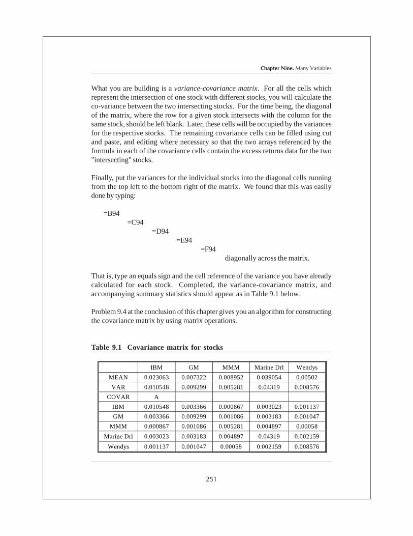
251
Chapter Nine. Many Variables
What you are building is a variance-covariance matrix. For all the cells whichrepresent the intersection of one stock with different stocks, you will calculate theco-variance between the two intersecting stocks. For the time being, the diagonalof the matrix, where the row for a given stock intersects with the column for thesame stock, should be left blank. Later, these cells will be occupied by the variancesfor the respective stocks. The remaining covariance cells can be filled using cutand paste, and editing where necessary so that the two arrays referenced by theformula in each of the covariance cells contain the excess returns data for the two"intersecting" stocks.
Finally, put the variances for the individual stocks into the diagonal cells runningfrom the top left to the bottom right of the matrix. We found that this was easilydone by typing:
=B94=C94
=D94=E94
=F94diagonally across the matrix.
That is, type an equals sign and the cell reference of the variance you have alreadycalculated for each stock. Completed, the variance-covariance matrix, andaccompanying summary statistics should appear as in Table 9.1 below.
Problem 9.4 at the conclusion of this chapter gives you an algorithm for constructingthe covariance matrix by using matrix operations.
Table 9.1 Covariance matrix for stocks
IBM GM MMM Marine Drl Wendys
MEAN 0.023063 0.007322 0.008952 0.039054 0.00502
VAR 0.010548 0.009299 0.005281 0.04319 0.008576
COVAR A
IBM 0.010548 0.003366 0.000867 0.003023 0.001137
GM 0.003366 0.009299 0.001086 0.003183 0.001047
MMM 0.000867 0.001086 0.005281 0.004897 0.00058
Marine Drl 0.003023 0.003183 0.004897 0.04319 0.002159
Wendys 0.001137 0.001047 0.00058 0.002159 0.008576

Part IV. Many Variables
252
Financial Modeling for Managers
General instructions for Excel matrix operations
When you construct your matrix in Excel, give it a name and make a note of whatit contains. The name must be placed in the cell directly above the top left handcorner of the matrix, which we have already done for the current data, putting thename A in cell [B92].
To perform matrix operations using the data you have set up, it is now necessaryfor you to formally notify the Excel program that the data you will be using exists ina named block of cells in your worksheet. You can do this as follows:
1. Using the mouse pointer, highlight the block of cells holding the input matrix.For purposes of the current application, this is the variance-covariance matrix,that is, cells B93:F97 if you followed our set up.
2. Run the mouse pointer up to the menu bar and click Insert, Name, Define...
3. The Define Name dialog box will appear. In the Names in Workbook inputbox, there should appear the letter A, the name you provided for your matrix incell [B92]. (If not, type in the name of your matrix.)
The Refers to: input box should list the range of your matrix. If it doesn't, clickin the box and edit using the delete and character keys to list the correct cells.For the present application this is B93:F97. Click [OK].
Now we are about ready to run. There are at least two methods for performingmatrix operations in Excel. The first method requires the least input time, but thesecond method might be easier for those of you who find the final keystrokecombination difficult.
If you get through Method 1, skip Method 2 and go directly to the following sectionon Mean-variance portfolios: solutions.
Matrix operations: Method 1
1. For the desired matrix operation, you must determine the order (i.e., dimensions)of the resulting matrix, and highlight the cells that it will occupy on yourspreadsheet.
2. With the "result" cells highlighted, type an equals (=) sign followed by the requiredmatrix command. (This could be, for example: =MINVERSE(A) )

253
Chapter Nine. Many Variables
Don't hit the [Enter] key at this point.
3. The simplest way to obtain the result matrix now is to strike three keys at once:
[Ctrl] + [Shift] + [Enter]
(Press [Ctrl] and [Shift] using your left hand, and while they are held down,then press [Enter]).
Matrix operations: Method 2
1. As with Method 1, for the desired matrix operation you must determine theorder (i.e. dimensions) of the resulting matrix, and reserve those cells on yourspreadsheet.
2. In the row directly above your result matrix, type the number one (1) in the farleft cell, followed by two (2) in the next column, and so on for the requirednumber of columns. (These cells provide the column references).
3. In the column directly to the right of your result matrix location, type the numberone (1) in the first row, two (2) in the second, and so forth down to the finalrow. (These cells will provide the row references).
4. In the top left cell of the result matrix, type your formula in the following format:
=INDEX(name of the Excel matrix operation [e.g. MINVERSE] (nameof the input matrix [e.g. A, as we have chosen]), row reference, columnreference).
Suppose, for example, that your result matrix is to rest in cells B123:F127.One possible layout is shown below, with cell contents designated in bold andcell names in italics.
A122
1
2
3
4
5
1
B123
C123
D123
E123
F123
2
B124
C124
D124
3
B125
D125
4
B126
5
B127
F127

Part IV. Many Variables
254
Financial Modeling for Managers
To obtain the result of the matrix operation for cell B123, into B123 we wouldtype the formula:
=INDEX(Matrix operation(matrix name),$A123,B$122)
If this command is copied into cell [B124], it will automatically change to:
=INDEX(Matrix operation(matrix name),$A124,B$122),
which is exactly what we want. Pasted into [C123], it will give:
=INDEX(Matrix operation(matrix name),$A123,C$122), correctly again.
In fact, the formula will provide the correct row and column references if cut andpasted throughout the result matrix. It is a bit of an effort to set up, but in doing so,you have learned something quite useful about cell referencing, in addition to avoidingthe three-at-a-time keystroke combination.
Performing a matrix operation without the three-at-once keystroke combinationwill generate an answer which includes only the top left hand element for the resultmatrix from the operation. The Index command provides a way to access theremaining elements of the result matrix.
Mean-variance portfolios: solutions
Having set up the covariance matrix, the next task is to generate the mean-varianceportfolios of Section 9.4. We'll use Method 1 to perform matrix operations, but youcan apply Method 2 just as easily.
A. Starting with the Minimum Variance portfolio, we first have to find the inverseof the covariance matrix, Σ-1. Begin by highlighting a 5 x 5 block of cells a fewcells below the original covariance matrix. (We used cells [B100] to [F104].)Type:
= MINVERSE(A) into the top left hand cell of the highlighted block.
Then press [Ctrl] + [Shift] + [Enter].
With a bit of luck, you will have created the new matrix, Σ-1, which appearsas Table 9.2.

255
Chapter Nine. Many Variables
Table 9.2 ΣΣΣΣΣ-1
108.9531 -36.464 -5.87672 -3.841636 -8.63143
-36.464 124.941 -14.5443 -4.592299 -8.2745
-5.87672 -14.5443 214.937 -22.57479 -6.2945
-3.84164 -4.5923 -22.5748 26.5248 -4.08114
-8.63143 -8.2745 -6.2945 -4.081138 120.2174
Referring back to Equation (4), we must now multiply Σ-1 by the vector 1. Theeffect of this multiplication is the same as adding across the columns of Σ-1,row by row. We can do this very easily on the worksheet. Check that youobtain the vector shown as Table 9.3.
Table 9.3 Σ-11
54.13937
61.06588
165.6467
-8.56506
92.93585
By summing the five elements of the vector Σ-1 1, we obtain the scalar (ordinarynumber):
1'Σ-1 1 = 365.2227
The vector of weights for the five securities is then obtained via Equation (4)as:
x = ,111
1 11
-- Σ
Σ′

Part IV. Many Variables
256
Financial Modeling for Managers
that is, by multiplying the vector Σ-1 1, by the inverse of the scalar above.This is easily done on the spreadsheet to give Table 9.4:
Table 9.4 (1 / 1'Σ-1 1) * Σ-1 1
0.148237
0.167202
0.45355
-0.02345
0.254464
Clearly, the Minimum Variance portfolio is heavily weighted towards the MMMstock and Wendy's - by just over 70%. The minus sign next to the fourthweight indicates shorting a small amount of the Marine Drill stock.
B. For the CAPM portfolio, we again use the inverse of the covariance matrixΣ-1, that we produced for the first portfolio above.
Following Equation (5), we must next multiply by µµµµµ, the vector of the stockmean (excess) returns. You must first create the vector as a column of fiveelements which we did as:
=B90=C90=D90=E90=F90
These are the cell references for our original calculation of the return means.
This produces the required vector:
µµµµµ =.
.
.
.
.
00502.
039054
008952
007322
023063

257
Chapter Nine. Many Variables
Use the Excel function MMULT (matrix multiplication) to compute Σ-1 µµµµµ. Toperform this function, first highlight a column of five empty cells for the resultvector. Into the top cell type:
= MMULT (cell range for Σ-1, cell range for stock means),
which on our worksheet was:
= MMULT($B$100:$F$104,$H$90:$H$94).
Then strike the combination: [Ctrl] + [ Shift] + [Enter], to produce:
Σ-1 µµµµµ = .
−
128052.0
691117.0
768771.0
277177.
999821.1
The front end of the right hand side of Equation (5), 1'Σ-1 µµµµµ, is just the sum of theelements of the vector Σ-1 µµµµµ, that is, the scalar which, for the data selected, comesto:
1'Σ-1 µµµµµ = 3.310584
The vector x of the weights for the selected securities to the CAPM portfolio isthen:
x = . --
µµ Σ
Σ′1
11
1
Its solution is given by:
x =.
03868.0
20876.0
232216.0
083724.0
604069.0
−

Part IV. Many Variables
258
Financial Modeling for Managers
This time the portfolio weights indicate a high proportion of our capital in IBMshares (60.4%), while we are directed to short sell a small amount of GM (amountingto 8.4% of our capital amount).
Finally, we will actually calculate the mean excess return of the two portfolios,again on an historical basis, and also their standard deviations. The standard deviationof the portfolio is sometimes called the capital at risk in portfolio managementliterature.
The variance of each portfolio excess return is calculated as:
σ2p = x' Σ x ,
while the mean excess return is computed as:
µp = x' µµµµµ .
The results of these computations for the two portfolios are shown as Table 9.5below. As you can see, the Minimum Variance portfolio (A) ended up with astandard deviation of about 62% of the CAPM portfolio (B), while its mean excessreturn was less than one-half of that achieved with portfolio (B).
Table 9.5 σσσσσp , µµµµµp
Portfolio
σ2
p
σp
µp (A) Minimum Variance
.002738
.052326
.009065
(B) CAPM
.007172
.084689
.023744

259
Exercises
91. (i) Determine which of the following matrix products can be found, and find
them.
. = C = B = A
43
01
21
,21
11,
243
501
112
(a) AB (b) AC (c) CA (d) CB (e) BC
(ii) Suppose that you have an N x 1 vector 1, whose every element consists ofthe number one (1). Now take a set of sample observations on somerandom variable x, namely x
1 , x
2 ,....x
N, and assemble them into a column
vector x. What does the product 1’x look like? The vector 1 is called thesummation vector – it does the same thing as the Σ sign.
2. In Section 9.2 you will find an answer to the inverse of the matrix below.Check that answer is correct using Excel (See Section 9.5).
5 = A
243
01
112
3. Consider the following set of equations:
2x1 + x2 + 2x3 = 1
x1 = 2
3x1 + 4x2 + 8x3 = 1
(i) From first principles, try to solve it. Does this set have a unique solution?
(ii) Write the set of equations in matrix-vector form.
(iii) Relate the solution problem to the linear dependence of the system matrix.

260
Exe
rcis
es 9
4. Here are some useful manipulations with statistical applications.
(i) Suppose that you have a N × k matrix of N observations on each of krandom variables. This is often called a data matrix. What does thematrix X'X contain?
(ii) Show that the sample covariance matrix can be cast in matrix-vector formas:
'xx- XX N
1 = ′Σ
where x is the vector containing the sample means.
5. Following the practicum of Section 9.5, you could try the following:
(i) Pick a set of five stocks that you think will show nicely complementaryproperties for purposes of diversification. Then repeat the procedures ofthe text; compute the CAPM portfolio and see if the portfolio dominatesthat of the text, in the sense that it has a higher mean return and a lowervariance.
(ii) Now get more ambitious and repeat the text exercise but with all 14 stockson board. The hardest part—aside from darting back and forth across thespreadsheet—is to assemble the covariance matrix of returns. To speedthings up, you might try the implied procedure in Q4 above, and do thewhole assemblage in matrix -vector operation.
Has the extra diversification improved the expected return- risk trade off,for either of the portfolios— the Minimum Variance or CAPM?

261

262

263
Part FiveAPPENDIX
General Mathematical Review
264
App
endi
x
A1 Order of operations
As it is frequently necessary for the financial manager to perform chains ofcalculations, it is important to know the correct order in which to execute the varioustypes of operations.
For example, if you are required to evaluate:
A = 8 - 4 × 3 ÷ 6 + 2 × 22 ,
where do you begin? Note that this is not just a simple matter of working from leftto right! There are standard rules governing the order in which we perform thevarious arithmetic operations.
Rules
1. Calculations within parentheses are performed first.2. Powers operations come next.3. Divide and multiply are next.4. Then add and subtract operations follow.
Where no brackets appear in the original equation, it is often easiest to start bygrouping the ÷, × and powers operations using parentheses.
A = 8 - 4 × 3 ÷ 6 + 2 × 22
= 8 - (4 × 3 ÷ 6) + (2 × 22)= 8 - (2) + (2 × 4)= 6 + 8= 14
Example A.1

265
AppendixA2 Multiplication and division with signed numbers
Numbers in calculations may be either positive or negative. When performingmultiplication or division, if the two operands have the same sign the answer ispositive. If they have different signs, then the result will be negative.
positive × positive = positivepositive ÷ positive = positivenegative × negative = positivenegative ÷ negative = positivenegative × positive = negativenegative ÷ positive = negative
Find C for:
C = -16 × -4 - 2 × -6 + 3 × -2 × -5
First group the operations of multiplication and division using parentheses:
C = (-16 × -4) - (2 × -6) + (3 × -2 × -5)
Solve for sign within each set of parentheses:
C = (16 × 4) - -(2 × 6) + (3 × 2 × 5)
Example A.3
B = 1 ÷ 3 × (4 + 5)2 - 7= 1 ÷ 3 × (9)2 - 7= (1 ÷ 3 × 81) - 7= (27) - 7= 20
Example A.2
266
App
endi
x
Calculate:
D = -24 ÷ -2 × 4 -5 × -8 ÷ -2 -12 - (5 × -1)
Group multiplication and division:
D = (-24 ÷ -2 × 4) - (5 × -8 ÷ -2)-12 - (-5)
Solve for sign within the brackets:
D = (24 ÷ 2 × 4) - (5 × 8 ÷ 2)-12 + 5
Perform the calculations within each bracket working from left to right:
D = (48) - (20) -7
= 28-7
= -4
Example A.4
Perform the calculations within each set of parentheses working from leftto right:
C = 64 + 12 + 30= 106

267
Appendix
Rules for indices
1. Numbers with indices can only be added or subtracted when they have thesame base and the same index.
Exercises
Find: E = 14 ÷ (-7) + 6 - 3 × 4 12 ÷ 6 – 4
F = 4 × 6 − (-12 ÷ (-2)) + 2 × 3 12 ÷ 3 + 5
2 × 2 × 2 × 2 × 2 = 25 .
Read as “2 to the power 5” where 5 is called the index, power or exponentand 2 is the base. In the above example the base “2” is multiplied by itselffive times.
Example A.5
A3 Powers and indices
Powers, indices and exponents are equivalent terms describing a shorthand wayof writing repeated multiplication. They are frequently used in compound interestcalculations.
a3 + a3 = 2a3
Example A.6
b + 6b + 8b = 15b
Example A.7

268
App
endi
x
E = 8x2 + 7y2 + 3x3 - 4y2 - 2x2
= (8x2 - 2x2) + (7y2 - 4y2) + 3x3
= 6x2 + 3y2 + 3x3
Example A.8
a3 × a2 = (a × a × a) × (a × a)= (a × a × a × a × a)= a5 .
that is: a3 × a2 = a3+2 = a5
Example A.9
F = a4 ÷ a3
F = a × a × a × a a × a × a
When all the numbers in the numerator and denominator are multiplied, it ispossible to reduce the equation as follows:
F = a × a × a × a a × a × a
(Note that this does not work if there is addition or subtraction in thenumerator or the denominator.)
Example A.10
2. Numbers with the same base but different powers can be multiplied. Theresult is the sum of the powers.
3. Division with Power Functions (Indices)

269
Appendix
4. Powers of Powers
When a number is raised first to one power (index), and then to another power,the indices are multiplied.
In the above example, we are left with the simplified form:
F = a
That is:
a4 ÷ a3 = a4-3 = a1 = a
Rule: When dividing numbers with the same base but different powers,subtract the indices.
a a a a a a = a a = a =G 3 ×××××× )()()( 323
. a = a 3 223)( ×∴
Example A.11
. a = a = a a a = a = H + + 2322222232 )( ×××
Example A.12
Caution:
)( 328)2( 3
a a = a ≠
Example A.13

270
App
endi
x
5. Negative Powers
A non-zero base raised to a negative power is the reciprocal of the baseraised to the same (positive) power.
6. Zero Power
Any non-zero base raised to the power of 0 (zero) has the value 1.This is because:
. = a so a = a
a =n
n
1;1 00
7. Fractional Indices
Problems with fractional indices are common when you are trying to compareinterest rates quoted with different compounding periods to determine theireffective return.
Rule: The value of a positive base raised to a fractional power, n, is equal tothe nth root of the base.
x1/n = n/x
101/2 = 2/10
10-1 = 1 2-5 = 1 x-n = 1 101 25 xn
Example A.14

271
Appendix
Solve for x:
(1 + x)4 - 1 = 0.16
Add one (1) to both sides:
(1 + x)4 = 1.16
Take the 4th root of both sides:
1 + x = 1.161/4 = 1.16.25 = 1.03780199
Subtract one (1) from both sides:
x = .03780199
Expressed as a percentage:
x = 3.780199%
Note on Simplifying Fractions
To simplify expressions with a fraction in the denominator, use the “invertand multiply” rule.
3 /4 = 3 ) 44 /5 4 5
Using the “invert and multiply” rule this can be rewritten as:
3 × 5 = 3 × 5
= 15
4 4 4 × 4 16
Example A.15

272
App
endi
x
A4 Logarithms
The logarithm, with base b, of a positive number A, is the power y such that by =A. The logarithm is written as log
bA so that y = log
bA means by = A.
Examples
log10
100 = ? 102 = 100 therefore log10
100 = 2
log2 32 = 5 log
5 25 = 2 log
3 27 = 3
ln x = loge x
ln is the notation for natural logs. They have as a base, the importantmathematical constant e, the value of which is approximately 2.71828.These days, natural logs are almost universally used for calculationsemploying logarithms.
Rules
1. The logarithm of a product of two or more positive numbers is the sum of thelogarithms of the numbers. For example:
log (A H B) = log A + log B
2. The logarithm of a quotient of two positive numbers is the logarithm of thenumerator minus the logarithm of the denominator. For example:
log (A/ B) = log A - log B
3. The logarithm of a positive number raised to a power is the product of thepower and the logarithm of the number.
Examples
log (Ay ) = y log A
log (x2 / 3) = log x2 - log 3 = 2 log x - log 3

273
Appendix
A5 Calculus
Derivatives and differentials the easy way
Figure 1 below is a sketch of some more or less arbitrary function f(x) of a variablex. The value y = f (x) appears on the vertical axis. We are going to look at thebehavior of the function f in a neighborhood of a point indicated as x on the sketch.Specifically, consider a small perturbation
δx = x1 - x
At the point E, a tangent to the function has been drawn; this is the line ET. Thepoint E has the vertical coordinate y = f (x). The point Y has vertical coordinate y
1
= f (x1 ) .
Rule 3 is useful when solving for the power.
Since log (xy) = y log x, then y = log (xy) log x
Logarithms are extremely useful for finding answers to questions starting, “Howlong…?”
How long does it take to double your money at an interest rate of 12% p.a.compound?
We wish to find x in the equation:
1× (1 + .12)x = 2 ( 1 + .12)x = 2
Take natural logs:
x ln 1.12 = ln 2 (applying rule 3)x = ln 2 = 6.116 years
ln 1.12
Example A.16
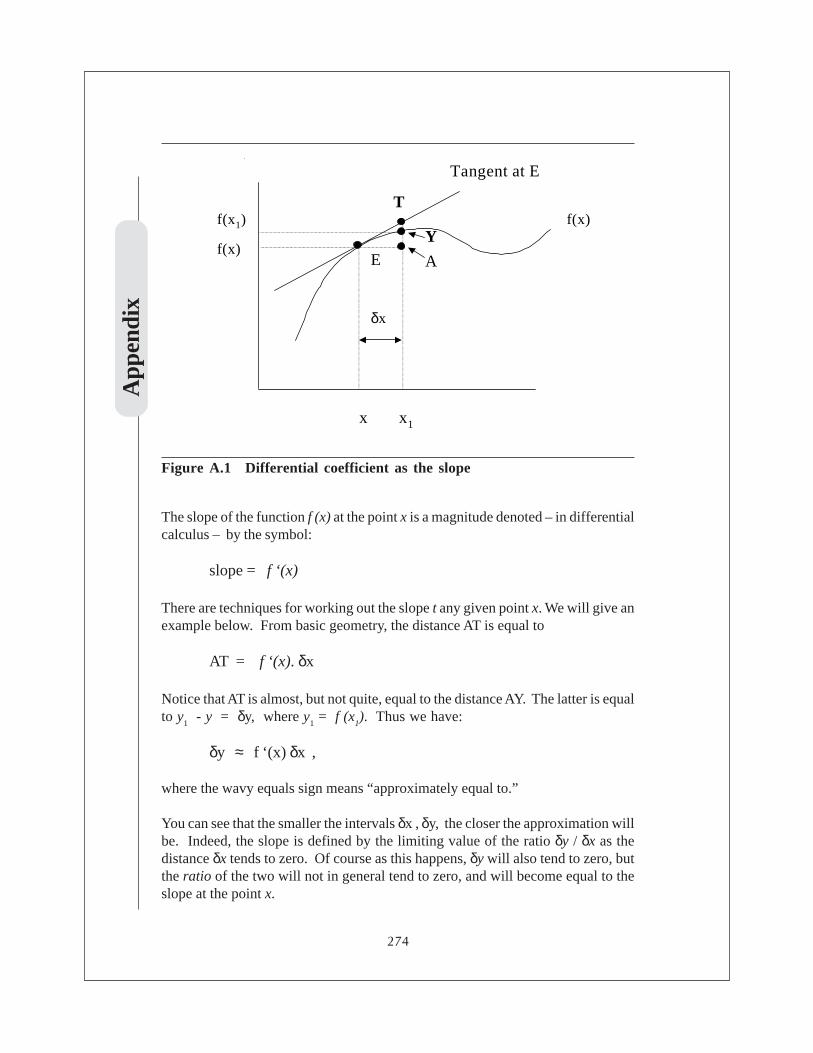
274
App
endi
x
The slope of the function f (x) at the point x is a magnitude denoted – in differentialcalculus – by the symbol:
slope = f ‘(x)
There are techniques for working out the slope t any given point x. We will give anexample below. From basic geometry, the distance AT is equal to
AT = f ‘(x). δx
Notice that AT is almost, but not quite, equal to the distance AY. The latter is equalto y
1 - y = δy, where y
1 = f (x
1). Thus we have:
δy ≈ f ‘(x) δx ,
where the wavy equals sign means “approximately equal to.”
You can see that the smaller the intervals δx , δy, the closer the approximation willbe. Indeed, the slope is defined by the limiting value of the ratio δy / δx as thedistance δx tends to zero. Of course as this happens, δy will also tend to zero, butthe ratio of the two will not in general tend to zero, and will become equal to theslope at the point x.
Figure A.1 Differential coefficient as the slope
E
Y
Tf(x)
x x1
Tangent at E
δx
f(x1)
f(x)A
275
Appendix
Conventionally, we use a special notation for the quantities δx, δy as δx 6 0. Wereplace δx by a thing called dx, and δy by something called dy, and we refer tothem as differentials. You might ask, “Why bother? Both are technically zero,”and this would be true. They are of the form of convenient fictional devices. If weknow the slope f ‘(x) at a particular point x, then we can use the equality:
dy = f r(x) dx, (1)
with the understanding that this represents the limit of an approximating process, inthe course of which the ratio of dy to dx becomes equal to the slope of the function:
. x f = dx
dy)(′ (2)
Differentials are heavily used in the mathematics of Ito processes (Chapter 8),again as a convenient shorthand. Indeed they are used in situations where theslope does not technically exist! In all cases, just think of them as small changes.
Techniques used to find the slope form the subject matter of differential calculus.There are certain basic results from which additional rules can be derived. Forexample:
If f (x) = a xn then (3a)
f ‘(x) = a × n xn-1 (3b)
To differentiate a power of x, you just lower the degree by one (1), and put theoriginal power out front. Constants like a in the above example make no difference.
Differential equations
Sometimes x can stand for time, so that we are dealing with functions of time. Inthis case we would write f(t). Suppose that someone said to you, “I know that theslope of a function, as t varies, is given by:
f ‘(t) = 12 t2 (4a)
Can you tell me what the original function must have been?”

276
App
endi
x
From expressions (3a), (3b), and employing t in place of x, the answer is:
f (t) = 4 t3 + c (4b)
How did we get this, and what does the constant c mean, anyway? The first termon the right hand side of (4b) was obtained by reversing (3b) to get the equivalentof (3a). In other words, if you differentiate the term 4t3, you get 12t2 which is thegiven expression (4a). The process of reversing the differentiation is called takingthe anti derivative, or more loosely, integration.
So far, so good. But how did the constant “c” sneak into the answer, and how dowe cope with it? When you differentiate a constant like c, the answer is alwayszero (ask yourself: what is the slope of a constant?). We could have started withany constant c in (4b) and still ended up with the given (4a). So we will have toallow for the possibility that there might have been some constant there anyway.To cope with the unpleasant feature of having some sort of indeterminate constanthanging around in our solution, we use any other information that might be availableabout the proposed function.
Suppose an informant had also told us that he knew that at time t = 0, the value ofthe function was f (0) = 10. For example, what was given to us as expression (4a)could be some sort of law of growth, referring to the rate of change of weight ofGodzilla. At birth, which is t = 0, it is known that Godzilla weighed ten tons. Oncewe know this information, we can set t = 0 in our proposed solution (4b) which nowtells us that the only qualifying constant is c = 10. So the complete solution for theweight of Godzilla at any time t is:
f (t) = 4 t3 + 10
We have solved the differential equation (4a). To do so, we have used as a pieceof further information that the value of f(t) at t = 0 is 10. The latter is a boundarycondition, or in this case, a particular form of boundary condition called an initialcondition.
Integration (briefly)
The antiderivative of a function is a much more general notion than the abovetreatment suggests. If you take an arbitrary function f(x), and antidifferentiate it,you end up with the integrated function F(x). This has the interpretation that at any

277
Appendix
point x, F(x) represents the area under f (x) to the left of the point x. Thus, integrationis associated with areas.
You can see where this might have application. If we have a formula for a probabilitydensity and integrate, or antidifferentiate it, you end up with the correspondingdistribution function, which is the cumulative area underneath the density.
Partial derivatives
Sometimes you may have a function of two variables rather than one. For example,for set values of parameters such as the strike price, the interest rate, and thevolatility, the value p of an option is a function of both the current stock price (S)and the time to maturity (t):
p = π (S, t )
We might be interested in the marginal effect of varying S while holding t constant.This is effectively the slope with respect to S. We might write it as:
partial slope wrt S = . S
∂∂ π
This is called the partial derivative with respect to S. To find it, you simply pretendyou are finding the ordinary derivative with respect to S, and treat t as a constantfor such purposes. Similarly, we can write:
partial derivative wrt t = . t
∂∂ π
If you are familiar with economics, you will be used to hearing that the total effecton the price p is a sum of the marginal effects, holding everything else constant.Suppose you observe small changes dS, dt in the values of S and t. Then the totalchange in p is given by:
. dt t
+ dS
S
= dp
∂∂
∂∂ ππ
(5)
Once you have worked out the partial derivatives, you know what the total effectis by summing the partial effects. As defined in (5), dp is called the total derivativeof the function π (S,t).

278
App
endi
x
Suppose a particular relationship between the partial derivatives were specified,for example, that the partial derivative with respect to t was equal to four times thepartial derivative with respect to S. What function π would have such a property?This is an example of a partial differential equation. It is rather similar to anordinary differential equation where there is only one argument varying, but thistime there are two. It is often possible to find a particular function p which wouldhave the required property. However the boundary conditions assume even greaterimportance, for there may be many functions that have the required property, butonly one that satisfies the designated boundary condition. For partial differentialequations, the boundary conditions often take the form of values of the function foran arbitrary S at a designated specific value T of t, the terminal value. For instance,the boundary condition for a call option is: At maturity t = T,
π = max ( S (T) - X , 0 )
For t < T, the call option price p does satisfy a partial differential equation, thoughit is a bit more complicated than the simple one mentioned above. But many otherderivative prices actually satisfy exactly the same equation, and it is necessary tospecify the boundary condition in the form given, in order to isolate the option price.
This completes our tour of calculus and differential equations.
279
Index
Index
A
Absolute addressing 131Annuity 32, 33, 36, 37, 49, 59, 70, 140, 141Annuity due 32, 33, 36, 38, 39Arbitrage 74, 79, 81, 83, 85, 88, 122, 217ARCH 204, 224, 225Ask 104, 107, 108, 111–113, 121
B
Bankers’ Acceptances 24Bid 111, 112, 121Bivariate data 177Bond equivalent yield 12, 14, 24, 25Bootstrapping 75
C
CD 24, 25, 27, 55, 56, 71, 154–156, 163, 249Commercial paper 12, 25Commodity currency 104–113, 119Compounding periods 10Continuous time 44–46, 97, 215, 218, 222Coupon 8, 13, 32, 47, 49--53, 59, 65, 70, 77, 78, 87, 89, 91, 93, 99, 100, 128,
130, 138--140, 142, 143, 146Covariance 244, 246–248, 250–252, 254, 256, 260Cross-rates 113
D
Degrees of freedom 170Density function 152, 165Direct Quotes 106Distribution 152, 153, 156, 159, 161, 166–173, 204, 213, 217, 226, 244, 246, 248Distribution function 152, 164, 165, 167, 219, 244, 277Drift 204, 215, 216, 218, 228Duration 31, 32, 57--61, 70, 100, 101
INDEX
280
Financial Modeling for Managers
E
Effective annual interest rate 32, 40Effective interest rate 8, 9, 32, 42, 45, 47, 59Equivalent rates 42Eurodollars 25Exchange rate 103–105, 107–114, 118, 120, 122
F
Fed Funds 26Fixed interest securities 47Forward 33, 61, 73, 75, 76, 80, 82, 84, 95, 96, 98, 100, 103, 104, 114,
116–120, 122, 206, 217Forward rates 81, 84, 86, 94, 96–98, 104, 114, 116Future value 11Futures 2, 12, 31, 33, 61–69, 71, 82, 84, 89, 144, 206–210, 212
Eurodollar Time Deposit 63, 7130-year T-bond 65, 66U.S. T-Bills 24
G
Generation process 152, 167, 170
H
Hedge 64, 71, 74, 82, 100, 119, 120, 207–209, 212, 219, 229Histogram 152, 153, 156–159, 161, 164, 167, 213Holding period yield 15, 25, 27
I
Implied forward 64, 73, 74, 79–81, 84, 86, 87, 97, 100, 118Implied volatility 204, 220–223Indirect quotes 106Inflation 8, 21, 22, 224Inversions 104, 108Invoice price 33, 52, 53, 62, 65, 66, 146IRR 33, 48, 74, 77, 87, 144Ito process 204, 215, 216, 218, 220
K
Kurtosis 152, 159, 161–163, 172Leptokurtic 152Platykurtic 152, 161, 163
281
Index
L
Linear interpolation 19, 28, 88Long 74, 81, 83
M
Macaulay duration 32, 57, 58, 70Martingale 204, 214, 220Matrix 155, 235–243, 245–249, 251–254, 256, 257, 259, 260Mean 97, 152, 153, 160–173, 204–207, 216–219, 223, 224, 228, 235, 243, 245–250,
252, 254, 256, 258, 260Mid-rate 104, 107, 108, 117Moment 41, 152, 160, 161, 167Money market securities 10, 12, 14, 24
N
Nominal 9, 39, 247NOW accounts 18Null hypothesis 169Number of days to maturity 8Numeraire 104, 105
O
OLS 207
P
Population 152, 153, 160, 161, 164, 166–168, 170–173Present value 8, 12–14, 16, 17, 24, 25, 32, 33, 35, 36, 38, 39, 47–49, 57, 70, 77,
118, 128, 135, 138, 140Present value of an annuity 33Present value of an annuity due 33, 36, 38Price 8, 12–15, 22, 24, 25, 27, 32, 34, 47–56, 59–65, 71, 74, 77, 78, 82–84,
88, 97, 103–105, 107, 108, 116–121, 139–141, 144, 146, 167, 203,204, 206, 209, 210, 212, 215, 217--219, 221, 223, 224, 226–230, 277, 278
R
Random sample 152, 153, 168, 226Random walk 204, 214, 227, 229Real interest rates 20Regression 149, 208, 209, 211, 212, 223, 225Relative addressing 131Repos 12, 25Reverses 12, 25
282
Financial Modeling for Managers
S
Sample 152, 153, 160–162, 164, 166–171, 173, 205, 214, 223, 226, 243, 248, 259,260
Short 74Sigma notation 51Simple interest 10, 11, 52Skewness 153, 159, 161Spot rate 74, 75, 79, 98, 116, 118, 119Spot rates 76, 80, 98, 104, 113Standard deviation 153, 160, 165, 168–170, 173, 208, 215–217, 228, 258Statistic 153Stochastic process 203–205Stochastic variable 204Swaps 87, 89Sweep accounts 18
T
Term structure of interest rates 73, 77Terms currency 104–107, 109, 119
U
U.S. T-Bill futures 61Unit-discount bond 74
V
Variance 152, 153, 160, 163, 166–168, 170, 171, 173, 204, 208, 213–216, 220, 223,224, 226–229, 235, 245–252, 254, 256, 258, 260
Vectors 235, 236
Y
Yield curve 19, 28, 71, 74, 77, 86, 89
Z
Zero coupon bonds 54, 78Zero coupon rates 57, 73, 74, 76, 77, 79, 80, 86, 88, 99, 100