WP/07/89

Financial Market Risk and U.S. Money Demand

Woon Gyu Choi and David Cook

© 2007 International Monetary Fund WP/07/89 IMF Working Paper IMF Institute

Financial Market Risk and U.S. Money Demand

Prepared by Woon Gyu Choi and David Cook1

Authorized for distribution by Jorge Roldos

April 2007

Abstract

This Working Paper should not be reported as representing the views of the IMF. The views expressed in this Working Paper are those of the author(s) and do not necessarily represent those of the IMF or IMF policy. Working Papers describe research in progress by the author(s) and are published to elicit comments and to further debate.

This paper examines empirically U.S. broad money demand emphasizing the role of financialmarket risk. We find that money demand rises with the liquidity risk of stock markets or the credit risk of corporate bond markets. After controlling for the effect of financial market risk, money demand becomes relatively stable over the last 35 years. At the sectoral level, household money holdings continue to be stable in a traditional model controlling for a decline in transactions costs for investing in mutual funds in the early 1990s. In contrast, business money holdings have been consistently (positively) associated with credit risk. JEL Classification Numbers: E41; E44; G10 Keywords: money demand; financial market risk; stock market liquidity; money market

mutual funds Authors’ E-Mail Address: wchoi@imf.org; davcook@ust.hk

1 Woon Gyu Choi is a Senior Economist at the IMF Institute of the International Monetary Fund. David Cook is an Associate Professor of Economics at the Hong Kong University of Science and Technology. We thank Shigeru Iwata and Jorge Roldos for useful comments and suggestions. We also thank In Choi and Timothy Chue for valuable conversations. Cook acknowledges the support of the HKUST RGC.

- 2 -

Contents Page I. Introduction ............................................................................................................................3

II. Data .......................................................................................................................................5 A. Measuring Financial Market Risk...............................................................................5 B. Measuring Money Balances, Opportunity Cost, and Income .....................................7

III. Financial Market Risk and Broad Money Demand ...........................................................10 A. Traditional Model and Financial Market Risk Model ..............................................10 B. Alternative Model Specifications with Different Sets of Risk Measures .................15 C. Out-of-Sample Forecast Using the Long-run Relationship.......................................17 D. Error Correction Model.............................................................................................20

IV. Sectoral Money Demand ...................................................................................................23 A. Household Money Demand versus Business Money Demand .................................23 B. Business Holdings of Quasi-Money..........................................................................27

V. Conclusion ..........................................................................................................................28

References................................................................................................................................30 Tables 1. Augmented Dickey-Fuller Tests ............................................................................................9 2. Cointegrating Vectors: Traditional Money Demand Model................................................11 3. Cointegrating Vectors: Financial Risk Models of Money Demand.....................................13 4. Cointegrating Vectors: Variations of Financial Risk Models of Money Demand...............16 5. Sub-Period Cointegrating Vectors: Variations of Financial Risk Models of Money Demand....................................................................................................................18 6. Error Correction Models of Money Demand with Financial Risk ......................................21 7. Cointegrating Vectors for Sectoral Money Holdings ..........................................................26 8. Cointegrating Vectors for Business Quai-Money Holdings ................................................28 Figures 1. Measures of Illiquidity, Liquidity Risk, and Default Risk.....................................................6 2. Movements in the Velocity of Money ...................................................................................8 3. Deviations from the Whole-Period Contegrating Vectors...................................................14 4. Deviations from the Sub-Period Contegrating Vectors .......................................................19 5. Dynamic Forecast of Money Demand using ECM..............................................................22 6. Money and Velocity in Household and Business Sectors............................................ 24 7. Velocity of Business Quasi-Money .....................................................................................27

- 3 -

I. INTRODUCTION

Broad money holdings have become substantially susceptible to financial market fluctuations since the early 1990s. During the late 1990s, broad money holdings rose sharply in the United States after many years of stagnation. A measure of real balances grew by about 1 percent per year in the 10-year period spanning 1987–1996, much slower than real output growth. A large literature at the time sought to explain the “missing” money demand (see Duca, 1993; Carlson and Keen, 1996; Feinman and Porter, 1992). By contrast, in the 9-year period spanning 1997–2005, real balances grew by about 5 percent per year. Since 1990, financial markets have been quickly changing and at times unstable. A decline in financial transactions costs may have promoted substitution between monetary assets and financial instruments. During much of the 1990s, U.S. blue chip stock prices were rising rapidly. During 1998–2001, there were sudden shocks to liquidity in international financial markets, which policymakers have explicitly linked to an increase in money demand (see Board of Governors, 2002).

In this paper, we argue that broad money holdings are part of the overall portfolio of

investors and are therefore susceptible to financial market risk. We estimate the U.S. money demand functions augmented with measures of risk in both stock and bond markets. We find that, after controlling for these financial market risk factors, money demand recovers stability.

The stability of money demand is important for the success of a monetary policy that

targets a monetary aggregate, because one cannot predict the effects of changes in the money supply on interest rates, income, and prices, without knowing the money demand function. However, amid rapid financial innovations since the mid-1970s, the empirical link between money and economic activity appears to have weakened, and the traditional money demand specifications become prone to instability (see Choi and Oh, 2003; Duca and VanHoose, 2004). The de-emphasis on monetary aggregates and the adoption of an interest rate policy rule have led to models of monetary policy in which money supply is infinitely elastic to the interest rate, and thus money becomes redundant in the presence of the interest rate, as noted by Leeper and Roush (2003). Nevertheless, a growing literature reveals a renewed interest in the role of money in the transmission mechanism (for example, Meltzer, 2001; Nelson 2002; Dotsey and Hornstein, 2003; Leeper and Roush, 2003).2 Further, understanding money demand in the context of portfolio allocation is increasingly important with the increased influence of financial instruments on the asset positions of households and businesses, which affect the sensitivity of money demand to financial market risk (Carpenter and Lange, 2003; Duca and VanHoose, 2004).

This paper examines a link between money demand and two measures of financial

market risk.3 The first measure is default risk in bond markets defined by the spread between the returns on low-rated debt and those on AAA-rated debt (Jagannathan and Wang, 1996). Money demand would increase with this risk if money were a relatively good substitute for bonds.

2 Meltzer (2001) emphasizes the real-world relevance of real balance effects. Nelson (2002) finds that real base money has a direct effect on real output independently of the short-term interest rate. Leeper and Roush (2003) show that money provides important information not contained in the federal funds rate. Dotsey and Hornstein (2003) suggest that money could be a useful indicator for a policymaker if money demand is more stable than it appears. 3 A large literature uses measures of aggregate risk based on both the dynamics and the cross section of conditional financial market returns (see Harvey, 1989; Cochrane, 2001).

- 4 -

The second measure is associated with stock market risk. There is a growing awareness

that substantial and persistent fluctuations exist in the systematic or aggregate liquidity of financial markets (see Amihud and Mendelson, 1986). Standard measures of market illiquidity such as the average bid-ask spreads (Chordia and others, 2000) or price impacts of trading levels (Amihud, 2002) change substantially over time and have negative impacts on aggregate stock returns. Pastor and Stambaugh (2003) and Acharya and Pedersen (2005) show that stock market illiquidity helps explain the cross-sectional variation of stock returns. Evidence from the asset pricing literature suggests that when markets are illiquid, investors are willing to pay higher prices to hold more liquid assets—implying that stock market illiquidity increases the holdings of more liquid, monetary assets. Fujimoto (2003) shows that macroeconomic shocks affect stock market liquidity. Choi and Cook (2006) examine the dynamic interactions between stock market liquidity and the macroeconomy for Japan. Their findings suggest that a decline in stock market liquidity leads to a rise in the demand for money.

There have been a number of periods in recent history when the traditional model has

persistently over- or under-predicted the demand for broad money. During the early 1990s, the demand for broad money fell sharply (see Duca, 1992; and Orphanides and Porter, 2000). Many authors connected this with increasing holdings of stock and bond mutual funds by households. It was argued that reduced transactions costs allowed for increased substitution for these assets. Some authors adjusted empirical money demand models to control implicitly (Carlson and others, 2000) or explicitly (Duca, 2000) for these changes. Others suggested including mutual funds in monetary aggregates (Collins and Edwards, 1994; Orphanides and others, 1994; Besci and Duca, 1994; and Duca, 1994, 1995). However, the reversal of the trend in money demand beginning around 1997 suggested that the previous efforts were incomplete.

In recent years, several papers have examined the short-run relationship between the stock market and money demand. Carpenter and Lange (2003) find that unexpected increases in stock market dividends reduce the demand for money. Dow and Elmendorf (1998) and Carlson and Schwarz (1999) find that both increases and decreases in stock returns have a positive effect on money demand. Duca (2003) find that the sensitivity of money demand to equity shocks is negatively associated with stock fund loads.

Our work is preceded by several other papers which emphasize the impact of

macroeconomic risk on money demand. Choi and Oh (2003) suggest that uncertainty about the future affects current money demand when the money stock must be chosen in advance of shocks to the economy. They examine the impact on macroeconomic uncertainty on narrow money demand to resolve several puzzles. The innovation here is the inclusion of asset pricing factors to represent uncertainty and risk. Carpenter and Lange (2003) find that a measure of implied stock market volatility is associated with long-run broad money demand in the late 1990s. Greber and Lemke (2005) use state space methods to derive an index of macroeconomic uncertainty to explain fluctuations in broad money demand (in the U.S. and Europe). By limiting ourselves to a small number of asset pricing factors, we not only avoid the challenges of constructed regressors in measuring uncertainty and risk but also find evidence that money demand has been sensitive to two well-recognized sources of financial risk.

- 5 -

Our results suggest that recent movements in money holdings are substantially attributable to financial market risk. Moreover, we find that money demand has become more sensitive to financial market risk in the last 20 years. To help understand this rising sensitivity, we focus on some changes in who is holding money. Traditional money demand theory has focused on the household sector’s money holdings. However, the business sector’s broad money holdings have been increasing since the 1970s. In 1970, the household sector held approximately $10 in broad money for every $1 held by the business sector. By 2005, that ratio dropped to about $3 to $1. We find that, conditional on a permanent level drop in money demand in the early 1990s, household money holdings have remained stable. In contrast, business money holdings have been growing rapidly and have become more sensitive to financial market risk. We suggest that the rising sensitivity of aggregate money demand to financial market risk is associated with growing money holdings by the business sector.

II. DATA

A. Measuring Financial Market Risk

We begin with a measure of aggregate stock market liquidity developed by Amihud

(2002).4 The illiquidity of stock j in month t is defined as the average ratio of the absolute value of the daily returns relative to turnover.

,

1 ,

1 tjDays

t njt j

t n t n

ReturnILLIQ

Days Turnover=

= ∑ (1)

where n = 1,2, 3…, Dayst represent the days of month t, ,

jt nReturn is the ex-dividend stock return

of security j on day n of month t, and ,j

t nTurnover is the value of shares traded (measured in millions of dollars). When a relatively small amount of market trading induces a relatively large change in the price of a stock, the stock market is thought to be relatively illiquid. The aggregate measure of stock illiquidity in month t is the average of j

tILLIQ

across a set of stocks, j = 1 to Jt, 1

1

t

t

Jj

t tJj

ILLIQ ILLIQ=

= ∑ . Following Pastor and Stambaugh

(2003), we include common stocks that were listed on the New York or American Stock Exchanges and had at least 10 observations in a given month. We include only shares with prices between 5 and 1000 dollars as those outside this range may have unusual liquidity patterns. We use daily data available from CRSP for November 1962–December 2005. This illiquidity measure is inherently non-stationary, declining overtime, because turnover grows with economic activity. Following Pastor and Stambaugh (2003) and Acharya and Pederson 4 Hasbrouck (2006) argues that this measure of stock market liquidity under some circumstances is associated with time-varying stock returns.

- 6 -

Figure 1. Measures of Illiquidity, Liquidity Risk, and Default Risk

.0000000

.0000005

.0000010

.0000015

.0000020

.0000025

.0000030

.0000035

1970 1975 1980 1985 1990 1995 2000 2005-14.0

-13.5

-13.0

-12.5

-12.0

-11.5

-11.0

-10.5

1970 1975 1980 1985 1990 1995 2000 2005

-14.0

-13.6

-13.2

-12.8

-12.4

-12.0

-11.6

1970 1975 1980 1985 1990 1995 2000 2005.004

.008

.012

.016

.020

.024

1970 1975 1980 1985 1990 1995 2000 2005

(A) ILLIQ (B) ILLIQUIDITY

(C) Liquidity Risk (D) Default Risk

Notes: The first row shows the time series of the cross-sectional average of the Amihud measure of illiquidity

(ILLIQt,) and the Amihud measure normalized by the lagged stock market capitalization (illiquidityt). The second row shows a two-year moving average of illiquidityt (Liquidity Riskt) and the spread between the interest rate on Moody’s seasoned BAA-rated corporate debt and the interest rate on Moody’s seasoned AAA-rated debt (Default Riskt). (2005), we normalize the series, multiplying tILLIQ by the stock market capitalization from 2 years earlier: 24ln( )t t tilliquidity ILLIQ MARKETCAP−= × .5

Figure 1 depicts ILLIQ and illiquidity at a quarterly frequency (averaging monthly observations). The measure, illiquidityt, has a substantial amount of high frequency variation. Sadka (2004) decomposes market liquidity into permanent and transitory components and finds that only permanent liquidity shocks are factored into asset prices. To abstract from this high frequency variation, we use an 8 quarter moving average of illiquidityt as a measure of liquidity risk: Liquidity Riskt = 71

8 0 t jjilliquidity −=∑ .

5 We normalize the illiquidity series by the lagged value of market capitalization to avoid the possible wealth effect of stocks on money demand in our regressions. Since dynamic estimations of regressions sometimes use 4 quarterly leads and lags of regressors, we lag the aggregate market capitalization by 2 years. The regression results are fairly similar if alternative lags of 12 or 6 months are used.

- 7 -

The Liquidity Riskt displays substantial and persistent variations in stock market liquidity,

as shown in the figure. The most liquid period in the stock market by far occurs during the bull market of the late 1960s. During the early 1970s, there are notable but temporary peaks of illiquidity during 1970 and following the 1973 oil shock. Stock market illiquidity was high during the period following the stock market crash in 1987 and the recession of 1990. The stock market becomes persistently illiquid following the 1998 LTCM/Russian crisis. The low point for liquidity occurs immediately following the terrorist attacks of 2001 though some recovery has been felt more recently. The standard deviation of liquidity risk is above 42 percent. An augmented Dickey-Fuller (ADF) unit root test with trend (and 7 lags chosen by the modified Schwarz criterion; see Ng and Perron, 2001) fails to reject a unit root (p-value=0.68), as reported in Table 1.

We also examine risk in the bond market. We use a very simple measure of default risk,

the spread between yields on BAA-rated bonds and the yield on AAA-rated bond, Default Riskt

= 1log( )1

BAAtAAAt

ii

++

. Figure 1 (panel D) shows a time series of default risk. A regression of Default

Riskt on a trend term shows that the variable has a small but statistically significant positive trend and has a mean of about 130 basis points with a standard deviation of about 30 basis points. There were sharp rises in default risk during the recessions in 1974 and also in the early 1980s when it reaches a peak of about 200 basis points. Following this, Default Risk falls sharply in the 1990s before rising again in the early 2000. An ADF test with trend (and no lags as chosen by the modified Schwarz criterion) fails to reject a unit root at the 10 percent level.

B. Measuring Money Balances, Opportunity Cost, and Income

To find the effect of financial market risk on money demand, we construct a broad measure of the money stock that includes monetary assets used both as substitutes for return-earning assets and for transaction purposes. Previous studies including Dow and Elmendorf (1998), Carlson and Schwarz (1999), and Duca (2003) identify money market mutual funds as potential gateways through which changes in stock market returns would affect money demand. We define a broad money supply, M2PF, which includes money market mutual funds as well as other components of broad money: M2PF = M2 + Institutional Money Market Mutual Funds (IMMMF). One notable measure of money, zero maturity money (MZM), includes large money market mutual funds on the grounds that they are checkable on demand. Unlike MZM, our measure (M2PF) includes small time deposits that have relatively high liquidity.6

The velocity of broad money was stable for the 1970s and 1980s but rose persistently during the first half of the 1990s and then fell sharply for 2000–2003. Monetary instability after 1990 seems to be largely associated with quasi-money (QM) holdings, because the velocity of narrow money (M1RS) remains relatively stable over the last 15 years. Quasi-money is defined 6 Earlier studies (Becsi and Duca, 1994; Duca, 1994; Duca, 1995) suggest that M2PF yields more accurate forecasts of inflation in the early 1990s than does M2 within the P-star (the long-run price level implied by a stable income velocity) framework (see, for the P-star model, Hallman and others, 1991). Some other studies show that the demand for MZM may be stable over time at least up until the expansion in money demand in the late 1990s (Carlson and Keen, 1996; Carlson and others, 2000).

- 8 -

Figure 2. Movements in the Velocity of Money

.40

.44

.48

.52

.56

.60

.64

.68

1970 1975 1980 1985 1990 1995 2000 2005.48

.52

.56

.60

.64

.68

.72

.76

1970 1975 1980 1985 1990 1995 2000 2005

1.5

1.6

1.7

1.8

1.9

2.0

2.1

1970 1975 1980 1985 1990 1995 2000 20050.65

0.70

0.75

0.80

0.85

0.90

0.95

1.00

1.05

1970 1975 1980 1985 1990 1995 2000 2005

(A) Velocity of M2PF (B) Velocity of M2

(C) Velocity of M1RS (D) Velocity of Quasi-Money

Notes: The first row shows the income velocity of M2PF (the sum of M2 and institutional money market funds)

and M2. The second row shows M1RS (M1 plus retail sweeps) and quasi-money (M2PF minus M1RS). as the difference between broad and narrow money: QM = M2PF – M1RS.7 Figure 2 depicts income velocity of money, defined by the money stock divided by nominal gross domestic product (GDP), in logarithm for alternative monetary aggregates from 1970 onward. A big surge in the velocity of M2PF and M2 in the 1990s reflects the reduced broad money holdings that were initially attributable to falling financial costs for investing in stock and bond mutual funds. However, in the late 1990s money velocity began to fall drastically reaching in 2003 a trough more than 20 percent below the level in the early 1990s. Although this velocity drift could conceivably be associated with interest rate movements, we show below that it is not fully explained by standard measures of the opportunity cost of money holding.

7 Our measure of narrow money, M1RS, is defined as: M1RS = M1+Retail Sweeps (see Dutkowsky and Cynamon, 2003). Retail Sweeps are transactions accounts to avoid statutory reserve requirements on transactions deposits (Anderson and Rasche, 2001; Anderson, 2003).

- 9 -

Table 1. Augmented Dickey-Fuller Tests

Variable ADF Test Statistics (p-value)

A. Risk Measures Liquidity Risk –1.84 7 Lags

(0.68) Default Risk –3.10 0 Lag

(0.10)

B. Monetary Aggregates Real Balances Opportunity Cost M2PF –2.10 7 Lags

(0.54) –2.95 2 Lags

(0.15) M2 –2.36 1 Lag

(0.40) –2.94 2 Lags

(0.04) M2M –2.23 1 Lag

(0.47) –2.22 2 Lags

(0.48) MZM –2.14 1 Lag

(0.56) –2.22 2 Lags

(0.48) C. Income Measures ln t

t

GDPP

–0.77 1 Lag

(0.97) ln t

t

PCEP

–0.45 3 Lags

(0.99) ln t

t

BSOP

–0.60 1 Lag

(1.00)

Notes: All tests include a constant and trend term. The number of lags, shown next to test statistics, is chosen by the Modified Schwarz criterion (Ng and Perron, 2001). P-values are in parentheses.

We measure the opportunity cost of holding each monetary aggregate as:

3

,

1log( )1

Mo TBillt

t Own Ratet M

ioci

+=

+, where 3 Mo TBill

ti is the annualized yield on 3 month treasury bills and

Own Rateti is the own rate on the aggregate. To calculate the own rate on individual asset j, we use

the following formula: usercostt,j = ,

1log( )1

BenchmarktOwn Ratet j

ii

++

, where Benchmarkti is the benchmark interest

rate used for the construction of the St. Louis Monetary Services Index (Anderson and others, 1997). For example, the own rate on M2PF is a weighted average of own rates on the

subcomponents: , 2 , , 2

22 2

Own Rate Own Rate Own Ratet tt M PF t IMMMF t M

t t

IMMMF Mi i iM PF M PF

= × + × . The own rate for IMMMF is

constructed from data on the user costs of IMMMF. The own rate on quasi-money is

, , 2 , 12 1Own Rate Own Rate Own Ratet t

t QM t M PF t M RSt t

M PF M RSi i iQM QM

= × − , where the own rate on narrow money, , 1Own Ratet M RSi , is

calculated as a weighted average of the own rates on currency, travelers checks, demand deposits, and other checkable deposits. The FRED database of the St. Louis Fed reports own rates for M2, M2M (M2 minus small time deposits), and MZM (M2M plus IMMMF).

- 10 -

The unit root hypothesis is not rejected at the 10 percent level for real balances, the opportunity cost defined above, and real income. Table 1 reports ADF test statistics and p-values with the lag selection chosen by the modified Schwarz criterion. In the ADF test for each series in logarithm, we include an intercept and trend term since there is strong evidence for a trend in each series. Real balances are defined by /t tM P , where money stock Mt is measured by one of the broad monetary aggregates, and price level Pt is measured by the GDP deflator. Income is measured by real GDP for the aggregate economy, real personal consumption expenditure (PCE) for the household sector, and real business sector output (BSO) for the business sector.

III. FINANCIAL MARKET RISK AND BROAD MONEY DEMAND

A. Traditional Model and Financial Market Risk Model

We first estimate a traditional money demand function:

0 1 2ln lnt tt t

t t

M GDP ocP P

β β β ω= + ⋅ + ⋅ + (2)

where Mt is a monetary aggregate, GDPt is quarterly nominal GDP, Pt is the GDP deflator, and the opportunity cost is oct , as defined in the previous section. The transaction and precautionary motives of money demand suggests the income elasticity, β1, far less than 1.0, whereas the quantity theory of money (Friedman and Schwartz, 1982; Hallman and others, 1991) or a general equilibrium monetary model (for example, Lucas, 2000; Choi and Oh, 2003) suggest a unitary income elasticity. Empirical studies tend to provide the income elasticity of broad money in the vicinity of 1.0 (see Sriram, 2001). Since our measure of oc is tantamount to a semi-log specification, β2 can be interpreted as the (long-run) interest semi-elasticity. The sign of β2 is negative, but the magnitude of β2 is not well guided by the theory or empirical studies—although the inventory-theoretic model suggests the interest elasticity of –0.5 (see Lucas, 2000). For broad money demand, Carlson and others (2000) find that the income elasticity is largely in the vicinity of 1.0, and the interest semi-elasticity is in the range of –2 and –6. Guerron (2006) finds the GMM estimate of the interest semi-elasticity as large as –12.62. The traditional money demand theory suggests a long-run relationship among the variables in equation (2). Given the evidence that these variables are integrated, we estimate a cointegrating vector for four broad monetary aggregates: M2PF, M2, M2M, and MZM. We compare two estimators: maximum-likelihood estimator based on a vector autoregression (VAR) system, following Johansen (1988); and dynamic ordinary least squares (DOLS), following Saikkonnen (1992) and Stock and Watson (1993). We choose the leads and lags in the DOLS estimator to optimize the AIC with a maximum of 4 leads and/or 4 lags. We choose the number of lags in the VAR to optimize the Schwartz information criterion with a maximum of 5 lags. For the DOLS estimators, standard errors are calculated using Newey-West estimates. We also report the Johansen trace statistic with the critical value at the 5 percent level, adjusted for sample size and number of lags (Cheung and Lai, 1993).

As opposed to the prediction of the traditional theory, however, we find no evidence on

the long-run relationship for all monetary aggregates. Table 2 reports the estimated cointegrating

- 11 -

Table 2. Cointegrating Vectors: Traditional Money Demand Model

Dependent Variable: Real Balances, ln( / )t tM P ; Sample: 1970:Q1–2005:Q4 Cointegrating Vector

ln t

t

GDPP oc t9094 Trace

Statistic Std. Dev. of

Coint. Vector M2PF A. Johansen (VAR: 2 Lags)

0.435* (0.219)

–33.108**(7.383)

23.12 (30.78)

0.303

B. DOLS (3 Leads, 1 Lag)

0.907** (0.032)

–4.972** (1.136)

0.056

M2 C. Johansen (VAR: 2 Lags)

0.516** (0.109)

–20.732** (3.856)

26.87 (31.30)

0.188

D. DOLS (4 Leads, 1 Lag)

0.747** (0.023)

–4.583** (0.836)

0.045

M2M E. Johansen (VAR: 5 Lags)

1.711** (0.247)

3.356 (4.629)

24.25 (32.38)

0.240

F. DOLS (4 Leads, 2 Lags)

0.849** (0.049)

–6.810** (0.717)

0.086

MZM G. Johansen (VAR: 5 Lags)

2.112** (0.304)

7.617 (5.679)

24.54 (32.38)

0.310

H. DOLS (1 Lead, 1 Lag)

1.065** (0.064)

–6.618** (0.806)

0.100

M2PF w/ t9094 I. DOLS (3 Leads, 1 Lag)

1.013** (0.043)

–4.044** (0.888)

–0.068* (0.034)

20.71 (44.37)

0.051

Notes: The estimated cointegrating vectors along with standard errors (in parentheses) are based on the Johansen and the Dynamic Ordinary Least Squares (DOLS) estimators. For the DOLS estimator, the Newey-West heteroscedasticity and autocorrelation robust standard errors are reported. We report the Johansen trace statistic for the null hypothesis of less than one cointegrating vector along with a 5% critical value (in parentheses). **, *, and † indicate significance at the 1%, 5%, and 10% level, respectively. vectors and contegration test results for the whole period 1970:Q1–2005:Q4. We are unable to reject the hypothesis of no cointegrating vector at even the 10 percent level with the Johansen trace statistic. The DOLS estimates are fairly consistent for all monetary aggregates: the income elasticity coefficient is positive and significantly below unity except for MZM, and the interest semi-elasticity is in the range of –4.5 and –7 and statistically significant at the 1 percent level. The Johansen coefficient estimates are much less coherent. The income elasticity estimates are near 0.5 for M2PF and M2 and much larger (close to 2.0) for M2M and MZM. The interest semi-elasticity is below –20 for M2PF and M2 but positive and insignificant for M2M and MZM.

- 12 -

Duca (2000) and Carlson and others (2000) emphasize that during the 1990s consumers experienced a permanent downward shift in financial transactions costs for investing in stock and bond mutual funds, leading to a drop in holdings of broad money. Given the lack of direct information on financial transactions costs, we also use the break linear trend, t9094, which is zero before 1990 and increases thereafter at a linear rate until it reaches 1 in 1995:Q1, as in Carlson and others. For the 1970–2005 period, however, the trace test fails to reject the hypothesis of no cointegrating vector, as reported in row I of Table 2. Nonetheless, the DOLS estimation of the cointegrating vector with t9094 as an exogenous, deterministic term yields that the income elasticity is remarkably close to one, and the interest semi-elasticity is –4.0. The coefficient on t9094 is negative and significant at the 5 percent level, suggesting that money holding decreased with the reduced financial transactions costs in the early 1990s.

We now introduce two financial risk factors to account for substitution effects in the

composition of the balance sheet or portfolio of assets. One factor is liquidity risk which contains information about the future course of returns on equity. As suggested by the liquidity preference theory and empirical evidence from the asset pricing literature, investors are willing to pay higher prices to hold more liquid assets when stock markets are illiquid. Another factor is default risk to account for substitutions between safe securities and risky securities. The emphasis of these factors reconciles the perspective of Friedman (Friedman and Schwartz, 1982, chapter 2) that money demand function includes returns on alternative assets as explanatory variables.8 We thus estimate our benchmark financial risk model given by

3 40 1 2ln lnt t

t t t tt t

M GDP oc Liquidity Risk Default RiskP P

β β β β β ω= + ⋅ + ⋅ + ⋅ + ⋅ + , (3)

where β4 and β5 are expected to be positive, since people substitute money for equity and bonds which entail less liquidity and higher credit risk than money. With the financial risk variables, we find evidence on the existence of a long-run money demand relationship and the unitary income elasticity of money. As shown in Table 3, cointegration tests reject the hypothesis of no cointegrating vector at the 5 percent (1 percent) level for M2PF and M2 (M2M and MZM). The coefficients on Default Riskt and Liquidity Riskt are positive and highly significant in most cases—consistent with our financial risk model predictions—except for the DOLS estimate of the coefficient on Liquidity Riskt for M2. The coefficient on Default Riskt tends to be greater for M2M and MZM for the Johansen than DOLS estimator. The income elasticity and interest semi-elasticity coefficients are more similar across the estimation methods than in the traditional model. In all cases, the income elasticity is close to one. We cannot reject the hypothesis of unitary elasticity at the 5 percent level for the Johansen estimates in most cases except for M2, while we can reject the hypothesis at the 5 percent level for the DOLS estimates in most cases but MZM.

8 We represent safe securities by AAA-rated bonds rather than Treasury bonds, given the liquidity differential between Treasury bonds and corporate bonds owing to, for example, the callability of corporate bonds (Duffee, 1998). The default risk variable is independent of the opportunity cost variable that is based on returns on risk-free assets. The liquidity risk variable contains significant information about the stock market, which is not included in the opportunity cost variable.

- 13 -

Table 3. Cointegrating Vectors: Financial Risk Models of Money Demand

Dependent Variable: Real Balances, ln( / )t tM P ; Sample: 1970:Q1–2005:Q4 Cointegrating Vector

ln t

t

GDPP

oc Default Risk

LiquidityRisk trend Trace

Statistic

Std. Dev. of Coint. Vector

M2PF A. Johansen (VAR: 1 Lag)

0.923** (0.043)

–7.024** (1.392)

8.219** (3.634)

0.107** (0.03)

75.36* (72.09)

0.088

B. DOLS (4 Leads, 3 Lags)

0.943** (0.027)

–5.217** (0.624)

16.493** (2.253)

0.072** (0.018)

0.068

M2 C. Johansen (VAR: 1 Lag)

0.786** (0.032)

–6.591** (1.053)

15.582** (2.842)

0.043† (0.023)

72.75* (72.09)

0.073

D. DOLS (4 Leads, 4 Lags)

0.788** (0.013)

–5.558** (0.519)

14.013** (1.625)

0.017 (0.01)

0.061

M2M E. Johansen (VAR: 1 Lag)

0.929** (0.068)

–9.729** (1.399)

25.988** (6.868)

0.102* (0.049)

86.23** (72.09)

0.153

F. DOLS (4 Leads, 2 Lags)

0.879** (0.043)

–5.742** (0.568)

6.944† (3.526)

0.102** (0.026)

0.088

MZM G. Johansen (VAR: 1 Lag)

1.083** (0.093)

–10.849** (1.905)

34.017** (8.983)

0.186** (0.066)

85.76** (72.09)

0.186

H. DOLS (1 Lead, 1 Lag)

1.062** (0.059)

–5.503** (0.727)

8.024** (4.379)

0.159** (0.037)

0.100

M2PF I. DOLS (4 Leads, 3 Lags)

1.749** (0.342)

–4.914** (0.718)

16.661** (2.171)

0.071** (0.019)

–0.006* (0.003)

91.49** (72.09)

0.058

Notes: The estimated cointegrating vectors along with standard errors (in parentheses) are based on the Johansen and the DOLS estimators. For the DOLS estimator, the Newey-West heteroscedasticity and autocorrelation robust standard errors are reported. We also report the Johansen trace statistic for the hypothesis of less than one cointegrating vector along with 5% critical values(in parentheses). **, *, and † indicate significance at the 1%, 5%, and 10% level, respectively.

Considering that stock market liquidity risk reaches a peak near the end of the sample, we check if our results could reflect a secular trend. Row I reports the DOLS estimates including a trend term. Since the inclusion of the trend term, which is significantly negative, roughly doubles the income coefficient, we concentrate on specifications without the trend term.9

9 With the trend term, the Johansen estimates of the cointegrating vector for both models become implausible.

- 14 -

Figure 3. Deviations from the Whole Period Cointegrating Vectors

-.3

-.2

-.1

.0

.1

.2

1970 1975 1980 1985 1990 1995 2000 2005

Traditional Financial Risk Note: The figure depicts (demeaned) deviations from the cointegrating vector (derived using the DOLS method)

from the financial risk model (solid line) and the traditional model (dashed line) for the 1970:Q1–2005:Q4 period. Why do the financial risk terms help recover stationarity of residuals from the

cointegrating vector? Notably, the estimates of income elasticity and interest semi-elasticity are similar across models. This means that differences in the behavior of the error correction (EC) term are largely attributable to the financial risk terms. The standard deviation of the EC term, residuals from the cointegrating vector, is much reduced when financial risk terms are included with the Johansen estimator but not so with the DOLS estimator. To have a closer look at this issue, we depicts in Figure 3 the EC term, ˆtω , after 1990 based on the DOLS estimator in the traditional and financial risk models for M2PF.

Turning to the details of the graph, the financial risk model outstrips the traditional model

after 1990. The traditional model persistently overpredicts money demand by 5–10 percent during the early- to mid-1990s. This pattern switches in the late 1990s. The inclusion of financial risk helps resolve these puzzles. During most of the 1990s, when the traditional model overpredicts money demand, equity markets had low liquidity, and default risk was relatively small. Indeed, while the financial risk model also overpredicts money demand, quantitatively the errors are much smaller and less persistent, compared to the traditional model. Later in the 1990s, financial risk rises, and money demand starts to increase. For 1998–2003, the financial risk model basically predicts money demand correctly, whereas the traditional model misses the sharp rise in money demand. In 2004, financial market risk appeared to fall dramatically but money demand did not. Thus, in the final 2 years, both models underpredict money demand.

- 15 -

Interestingly, however, the financial risk model does not fit well the data during the era when Regulation Q was in force.10 Large swings in our measures of financial risk in the 1970s did not drive fluctuations in money demand to the same degree as in the 1990s. As a result, the financial risk model has large and volatile error terms in the 1970s. For 1983–2005, the standard deviation of the EC term is less than 4 percent for the financial risk model and is about 6 percent for the traditional model. For 1970–1982, however, it is more than 10 percent for the financial risk model and is less than 5 percent for the traditional model. B. Alternative Model Specifications with Different Sets of Risk Measures

We consider alternative specifications of the financial risk model, especially introducing different sets of risk measures to see whether we can draw additional implications by doing so. The DOLS estimation results are summarized in Table 4. First, since accounting for financial risk substantially increases the ability of the model to explain money demand after 1990, excluding one of the two financial risk variables results in a lower model predictive power.11 In the model setting β3 =0, the coefficient on Default Risk is positive and significant at the 1 percent level (column A). Alternatively, in the estimated model setting β4 =0, the coefficient on Liquidity Risk is significant at the 5 percent level (column B).

Second, we introduce a stock premium in place of liquidity risk since the stock premium

in part reflects that equity has riskier returns and thus less liquidity than monetary assets.

Following Fama and French (1988), we define Stock Premiumt = 500

5

1ln( )1

DYt

GSt

ii

++

, where 500DYti is

the dividend yield on the S&P 500, and 5GSti is the yield on 5-year U.S. Treasury notes. An

increase in the expected risk of stock returns raises this variable, increasing money demand. However, holding risk constant, an increase in dividend yield should make stocks more attractive than money, reducing money demand. As reported in the table (column C), the coefficient on Stock Premium is positive and significant at the 1 percent level, indicating that the relative risk effect dominates the relative return effect.12

Third, we estimate alternative financial risk models with bond market risk measures. We

define 5

1log( )1

AAAt

t GSt

icorporate spreadi

+=

+ as the difference between the yield on AAA-rated

bonds and 5-year Treasury notes. This variable is more closely related to liquidity risk than to default risk. Column D reports a regression in which we substitute Corporate Spread for

10 Gilbert and Holland (1984) report that banks are allowed to offer competitive interest rates through money market deposit accounts in the first quarter of 1983. 11 The standard deviation of the EC term over the period 1990:Q1–2005:Q4 when neither financial risk variable is included is 0.071. The standard deviation is 0.057 (0.059) when only Default Risk (Liquidity Risk) is included and 0.042 when both variables are included. 12 Over the course of the sample period, the EC term for the financial risk model is very similar regardless of whether Liquidity Risk or Stock Premium is used: it has a slightly smaller standard deviation with the use of Stock Premium (0.063 versus 0.067), which leads to less overprediction of money demand for recent years.

- 16 -

Table 4. Cointegrating Vectors: Variations of Financial Risk Models of Money Demand

Dependent Variable = ln( 2 / )t tM PF GDP Variable A B C D E

ln t

t

GDPP

0.931** (0.030)

0.914** (0.029)

0.978** (0.023)

0.898** (0.026)

1.192** (0.017)

oct –6.867** (1.005)

–3.497** (0.947)

–3.594** (1.073)

–3.502** (1.165)

–2.615** (0.695)

Default Risk

12.973** (3.300)

18.927** (2.888)

11.509** (2.624)

38.816** (2.797)

Liquidity Risk

0.052* (0.023)

Stock Premium

2.562** (0.666)

Corporate Spread

6.090** (2.204)

Implied Volatility

–0.001 (0.001)

Leads/Lags 2/4 1/1 2/4 4/1 3/4

Trace Statistic Leg Length

51.35* (49.99) 2 lags

50.86* (49.09) 1 lag

81.15* (73.83) 1 lag __

70.11

(75.23) 2 lags

95.47*

(74.74) 1 lag

Notes: The estimated cointegrating vectors based on the DOLS estimator. Regressions A–D are estimated for 1970:Q1–2005:Q4, and regression E is estimated for 1986:Q1–2005:Q4. The Newey-West heteroscedasticity and autocorrelation robust standard errors are reported in parentheses. The Johansen trace statistics are reported for the hypothesis of less than one cointegrating vector along with 5% critical values (in parentheses). The leg length for the VAR-based Johansen estimator is chosen by the AIC. **, *, and † indicate significance at the 1%, 5%, and 10% level, respectively.

Liquidity Risk. The coefficient on Corporate Spread is positive and significant at the 1 percent level, but the trace test suggests no evidence on the existence of a long-run relationship.13

Finally, following Carpenter and Lange (2003), as a measure of financial risk, we use the

expected stock market volatility drawn from the application of the Black-Sholes model to an index of S&P 100 stock options of the Chicago Board of Options Exchange. Carpenter and Lange find that this measure, VXOt, is positively correlated with M2 money demand for 1995:Q4–2002:Q2. We estimate our financial risk model replacing Liquidity Risk with VXO for 1986:Q1–2005:Q4, being dictated by the availability of the measure only after the mid-1986 (column E). In this sample, however, this volatility measure is not statistically significantly associated with money demand.

13 Greber and Lemke (2005) suggest the spread between the AAA bond rate and a Treasury bill rate. Using the 3-month Treasury bill rate in place of the 5-year Treasury bond rate, however, resulted in an insignificant coefficient on this measure of corporate spread.

- 17 -

C. Out-of-Sample Forecast Using the Long-run Relationship

We are now interested in whether the long-run relationship implied by a model is helpful in predicting the swings of money demand that occurred after 1990. Given that the estimated income elasticity is close to one for the whole period, to compare the role of risk variables across time, we impose unitary income elasticity ( 1 1β = ) for the financial risk velocity model:

3 40 2

2ln tt t t t

t

M PF oc Liquidity Risk Default RiskGDP

β β β β ω= + ⋅ + ⋅ + ⋅ + , (4)

which also embeds the traditional velocity model by setting 3 4 0β β= = . The estimated velocity model for different periods using the DOLS and the Johansen methods are reported in Table 5. Regardless of the sample periods, we are able to reject the hypothesis of no cointegrating vector at the 1 percent level. For the full sample, which is also considered for comparison purposes, the coefficient estimates are very similar to those without the restriction of unitary income elasticity and close across estimation methods (rows A and B).

We then estimate the velocity model for 1970:Q1–1998:Q3, because the Russian crisis of

1998 seems to have sparked an increase in liquidity risk. Rows C and D show the results for the traditional velocity model with the dummy variable t9094 to account for a shift in the cost of investing in financial assets. The interest semi-elasticity is negative and significant and fairly similar across estimation methods. Rows E and F show the results for the financial risk velocity model. The DOLS estimates of the financial risk coefficients are significantly positive, although the effects of financial risk are not so pronounced as in the full sample. The Johansen estimates of the coefficients are all highly significant and remarkably similar to those from the full sample.

The financial risk model outstrips the traditional model in the forecast of money demand

after the 1998 LTCM/Russian crisis. Figure 4 shows the (demeaned) EC term of three models estimated using data for 1970:Q1–1998:Q3: the traditional velocity model without the dummy variable t9094; the traditional velocity model with t9094; and the financial risk velocity model. All the series are constructed using the DOLS estimator of the cointegrating vector. First, we see the traditional velocity model without t9094 misses the (in-sample) drop in money demand that occurred in the early to mid-1990s. Both the traditional velocity model with t9094 and the financial risk model do a reasonably good job of predicting the drop in money demand in this period. The EC term is near zero for both models during this period. However, when money demand begins to reverse after the third quarter of 1998, the traditional model with t9094 does a very poor job in the out-of-sample prediction of money demand, underpredicting money demand by about 15 percent after 2001. By contrast, the financial risk model underpredicts money demand only after 2003 with a much lesser degree than the traditional models do.

Would the financial risk model have predicted the initial decline in money demand that

occurred during the 1990s? In out-of-sample forecasts, we find that the financial risk model estimated for pre-1990 period is able to predict neither the early 1990s decline in money demand nor the late 1990s increase. This finding is based on the estimated model for 1970:Q1–1989:Q4

- 18 -

Table 5. Sub-Period Cointegrating Vectors: Variations of the Financial Risk Model

Dependent Variable = ln( 2 / )t tM PF GDP Cointegrating Vector

oc Default Risk

Liquidity Risk t9094 Trace

Statistic

Std. Dev. of Coint. Vector

Sample: 1970:Q1–2005:Q4 Financial Risk A. Johansen (VAR: 2 Lags)

–6.526** (1.415)

22.899** (3.856)

0.116** (0.033)

63.97** (49.09)

0.095

B. DOLS (4 Leads, 3 Lags)

–4.004** (0.724)

17.190** (2.502)

0.066** (0.015)

0.065

Sample: 1970:Q1–1998:Q3 Traditional C. Johansen (VAR: 1 Lags)

–1.881** (0.404)

–0.027** (0.007)

24.07** (15.55)

0.055

D. DOLS (1 Lead, 1 Lags)

–2.363 (0.269)

–0.130** (0.005)

0.019

Financial Risk E. Johansen (VAR: 1 Lag)

–6.755** (1.536)

23.051** (4.349)

0.136** (0.042)

57.27** (49.57)

0.106

F. DOLS (4 Leads, 3 Lags)

–2.799** (0.888)

15.106** (2.695)

0.043* (0.019)

0.060

Sample: 1970:Q1–1989:Q4 Financial Risk G. Johansen (VAR: 1 Lag)

–2.993** (0.321)

1.660 (1.086)

0.035 (0.008)

69.87** (50.37)

0.030

H. DOLS (4 Leads, 3 Lags)

–2.095** (0.456)

–0.081 (1.389)

0.026 (0.007)

0.022

Sample: 1970:Q1–2005:Q4

Financial Risk oc

d90-05 × Default Risk

d90-05 × Liquidity Risk

I. Johansen (VAR: 3 Lags)

–2.663** (0.704)

52.312** (5.117)

0.035** (0.003)

59.45** (52.21)

0.050

J. DOLS (4 Leads, 2 Lags)

–2.543** (0.329)

39.723** (2.793)

0.028** (0.001)

0.039

Notes: Cointegrating vectors are based on the DOLS estimator. The Newey-West heteroscedasticity and autocorrelation robust standard errors are reported in parentheses. The Johansen trace statistics for the hypothesis of less than one cointegrating vector are reported along with 5% critical values (in parentheses). **, *, and † indicate significance at the 1%, 5%, and 10% level, respectively.

- 19 -

Figure 4. Deviations from the Sub-Period Cointegrating Vectors

-.15

-.10

-.05

.00

.05

.10

.15

.20

1990 1992 1994 1996 1998 2000 2002 2004

Financial Risk TraditionalTraditional w/ t9094

Notes: This figure shows (demeaned) deviations from the cointegrating vector (using the DOLS method) from

the traditional and financial risk models estimated with data only up to the 3rd quarter of 1998. The traditional model is estimated without (dashed line) and with (dash-dotted line) a dummy variable, t9094, to control for the cost of investing in financial assets.

using the DOLS and Johansen estimators reported in rows G and H of Table 5. The cointegrating vector estimates are again similar across estimation methods, while the coefficient on Liquidity Risk is smaller than that for the full sample but still significant at the 1 percent level. The coefficient on Default Risk is essentially zero and insignificant. We are able to reject the hypothesis of no cointegrating vector, but this is not surprising since the traditional model itself rejects the same hypothesis. Previous work (see, for example, Hallman and others, 1991; and Hafer and Jansen, 1991) has found that broad money demand was stable before 1990.

Accounting for the increased sensitivity of money demand to financial risk in the 1990s

improves money demand predictability. We re-estimate the cointegrating vector using Liquidity Risk and Default Risk interacting with a dummy variable which equals 1 since 1990 and 0 before 1990 (rows I and J).14 The coefficients on the financial risk factors interacting with dummies—so that the effects of financial risk introduced only after 1990—are positive and strongly significant for both estimation methods.15 With this specification, the standard deviation of the cointegrating

14 We found the estimated income elasticity very close to one and could not reject the unitary income elasticity. 15 To check if the effect of financial risk is due to our omission of wealth effects from financial market on money demand, we estimate the regression that additionally includes the stock market capitalization deflated by the price level. The DOLS estimate of the coefficient on stock market capitalization is insignificant, while the effect of financial risk largely remain intact, suggesting that the financial risk variables are not masking the wealth effects.

- 20 -

vector is substantially smaller than traditional models or the financial risk models that assume that financial risk affects money demand evenly through time. D. Error Correction Model

So far we examined the long-run, cointegrating relationship for money demand. Since an error correction model (ECM) enables us to allow for a richer array of short-run dynamics as well as to reflect the long-run relationship, we consider a general form of ECM as follows:

1 2 3

0 1, 2, 3,1 1 1

5 4

5, 4, 11 1

2 2ln ln ln

ˆ

n n nt t k t

k k k tk k kt t k t

n n

k t k t EC t tk k

M PF M PF GDP ocP P P

Liquidity Risk Default Risk

γ γ γ γ

γ γ γ ω ε

−

= = =−

−= =

Δ = + ⋅Δ + ⋅Δ + ⋅Δ

+ ⋅Δ + ⋅Δ + ⋅ +

∑ ∑ ∑

∑ ∑ (5)

where 1ˆtω − is the lagged EC term from the DOLS estimator. The lag lengths of the model are chosen in the context of the general-to-specific approach. To control for an unprecedented contraction in the real balance (about 7 percent) during 2003:Q4, we introduce a dummy variable, D03Q4, which equals 1 at 2003:Q4 and zero at other periods.16

Liquidity risk seems to become more significant as financial costs fall. Carlson and others (2000) argue that financial costs fell dramatically during the early 1990s. To fully capture the contemporary impact of financial market risk on money demand, we estimate regressions for the period from 1993:Q1 to 2005:Q4 . We also conduct out-of-sample money forecasts based on regressions estimated for 1993:Q1–2002:Q4. For comparison purposes, we also estimate a traditional model. In both models, the hypothesis of no cointegration is rejected at the 1 percent level. Each ECM uses the cointegrating vector of the corresponding period based on the DOLS estimator (with 2 leads and 1 lag).

All variables enter the estimated ECMs with the signs expected by the theoretical model,

and the estimated ECMs attain a high level of goodness of fit and pass a battery of diagnostic tests for model specification. Table 6 summarizes the estimated ECMs.17 The adjusted R2 ( 2R ) of this parsimonious ECM is about 0.83 (0.80) for the financial risk (traditional) model. In the financial risk model (panel A), real balance growth is rather persistent, as shown by its coefficient of 0.36, and the coefficient on tocΔ is significantly negative. The coefficients on ΔDefault Risk and ΔLiquidity Risk are positive and significant at the 5 percent level. The coefficient of the EC term is –0.149 and significant at the 1 percent level, suggesting that about 15 percent of deviations from the equilibrium is corrected in the subsequent period. In the

16 The decline in M2 and M2PF during 2003:Q4 was the largest on record since the start of consistent data collection in 1959. The contraction was considerably concentrated in liquid deposits and might largely be attributable to the unwinding of a previous buildup in deposits associated with heavy mortgage refinancing activity (Federal Reserve Board, 2004). Our financial market risk model, however, can not incorporate such an effect because it does not account for housing market instruments. 17 The number of lags of real balances (n1) is chosen by the AIC. We include contemporaneous values of each of the variables and test whether an additional lag could be included. The coefficients on GDP growth and additional lags of changes in opportunity cost were not significant at the 10 % level and thus not included.

- 21 -

Table 6. Error Correction Models of Money Demand with Financial Risk

Sample Period: 1993:Q1–2005:Q4 A. Financial Risk Model

-1 -1ln( 2 / ) 0.002 0.020 03 4 0.363 ln( 2 / ) 1.911 0.021 (0.002) (0.005) (0.084) (0.297) (0.009)

ˆ 1.893 0.149(0.808) (0.049)

t t t t t t

t

M PF P D Q M PF P oc Liquidity Risk

Default Risk

Δ = − + Δ − Δ + Δ

+ Δ − 1tω −

ˆ ln ( / ) 2.420 1.296 ln( / ) 4.767 0.062 6.353 (0.191) (0.012) (0.277) (0.008) (1.850)

M P GDP P oc Liquidity Risk Default Riskω = + − + − −

2R =0.831, SE=0.436%, DW=2.03, 1(2)ξ =0.82 (0.66) )4(1ξ =2.45 (0.65)

2(2)ξ =1.32 (0.52), )4(2ξ =3.22 (0.52), )2(3ξ =1.91 (0.38), 4(2,43)ξ =2.94 (0.06) Within-sample dynamic simulation for 1993:Q1–2005:Q4: ME = –0.0002, RMSE = 0.008 B. Traditional Model

-1 -1 1ˆln( 2 / ) 0.001 0.024 03 4 0.530 ln( 2 / ) 2.157 0.068(0.002) (0.005) (0.072) (0.336) (0.029)

t t t t t tM PF P D Q M PF P oc ω −Δ = − + Δ − Δ −

ˆ ln ( / ) 4.142 1.410 ln( / ) 7.961(0.249) (0.027) (0.664)

M P GDP P ocω = + − +

2R =0.802, SE=0.472%, DW=2.06, 1(2)ξ =1.92 (0.38), )4(1ξ =5.34 (0.25)

2(2)ξ =0.62 (0.73), )4(2ξ =7.41 (0.12), )2(3ξ =8.02 (0.02), 4(2,45)ξ =2.54 (0.09) Within-sample dynamic simulation for 1993:Q1–2005:Q4: ME= –0.003, RMSE = 0.014

Sample Period: 1993:Q1–2002:Q4 C. Financial Risk Model

-1 -1

1

ln( 2 / ) 0.0002 0.360 ln( 2 / ) 2.169 0.041 (0.002) (0.085) (0.299) (0.012)

ˆ 1.711 0.184(0.865) (0.058)

t t t t t t

t t

M PF P M PF P oc Liquidity Risk

Default Risk ω −

Δ = + Δ − Δ + Δ

+ Δ −

ˆ ln ( / ) 1.984 1.260 ln( / ) 4.743 0.070 5.080 (0.358) (0.031) (0.329) (0.010) (1.423)

M P GDP P oc Liquidity Risk Default Riskω = + − + − −

2R =0.860, SE=0.402%, DW=2.20, 1(2)ξ =3.14 (0.21), )4(1ξ =4.29 (0.37)

2(2)ξ =1.29 (0.53), )4(2ξ =3.09 (0.54), )2(3ξ =1.32 (0.52), 4(2,32)ξ =1.56 (0.23) Out-of-sample dynamic forecast for 2003:Q1–2005:Q4: ME = –0.008, RMSE = 0.022 D. Traditional Model

-1 -1 1ˆln( 2 / ) 0.0004 0.505 ln( 2 / ) 2.234 0.082(0.002) (0.084) (0.345) (0.030)

t t t t t tM PF P M PF P oc ω −Δ = + Δ − Δ −

ˆ ln ( / ) 4.469 1.446 ln( / ) 6.920(0.193) (0.021) (0.572)

M P GDP P ocω = + − +

2R =0.813, SE=0.465%, DW=2.03, 1(2)ξ =1.52 (0.47), )4(1ξ =6.62 (0.16)

2(2)ξ =0.69 (0.71), )4(2ξ =5.39 (0.25), )2(3ξ =6.78 (0.03), 4(2,34)ξ =3.58 (0.04) Out-of-sample dynamic forecast for 2003:Q1–2005:Q4: ME= 0.020, RMSE = 0.023 Notes: Error corrections terms are based on the cointegrating vectors estimated by the DOLS method. The

numbers in parentheses below coefficient estimates are the Newey-West heteroscedasticity and autocorrelation robust standard errors. 2R is the adjusted R2; SE is the standard error of the regression in percent; DW is the Durbin-Watson statistic; ξ1(i) is Lagrangian Multiplier (LM) version of χ2 test for i-th order serial correlation; ξ2(i) is the LM version of χ2 test for autoregressive conditional heteroscedasticity (ARCH) of i-th order; ξ3(2) is the Jarque-Bera χ2 (2) test for normality; and ξ4(2, degree of freedom) is the F-statistic of Ramsey’s RESET test. P-values are in parentheses following the test statistics.

- 22 -

Figure 5. Dynamic Forecast of Money Demand using ECM

-.02

-.01

.00

.01

.02

.03

.04

93 94 95 96 97 98 99 00 01 02 03 04 05

ActualFinancial Risk ModelConventional Model

(A) Within-Sample Dynamic Forecast: 1993:Q1-2005:Q4

-.02

-.01

.00

.01

.02

.03

.04

2000 2001 2002 2003 2004 2005

ActualFinancial Risk ModelConventional Model

(B) Out-of-Sample Forecast: 2003:Q1-2005:Q4

Note: Dynamic forecasts for Δln(M2PF/P) are based on the ECMs reported in Table 6.

traditional model (panel B), real balances are more persistent with a coefficient on lagged real balances growth as high as 0.54. The coefficient on the EC term is –0.068 and significant at the 5 percent level, smaller and less significant than that of the financial risk model.

The ECM for the financial risk model passes tests for serial correlation, autoregressive conditional heteroskedasticity, and normality, while that for the traditional model does not pass normality at the 5 percent level. Both models marginally pass the RESET test for functional form specification at the 5 percent level. We also find that the cumulative sum (CUSUM) test and the CUSUM squares test do not reject structural stability at the 5 percent level for both models. Further, we find that Hansen’s (1997) procedure of the structural-change tests for the ECM, which account for the uncertainty surrounding the date of the structural break, suggests a high stability for both the financial risk and the traditional models.18

Within-sample dynamic forecasts for 1993:Q1–2005:Q4 suggest that the estimated ECMs

have precise predictions over time and a high level of dynamic stability—the financial risk model outstrips the conventional model. The forecasts of the financial risk model deviate from the real balance only by 0.02 percent in terms of mean error (ME) and 0.8 percent in terms of RMSE (root mean squared error). The forecasts of the traditional model deviate from actual real balances by a greater amount compared to those of the financial risk model: 0.3 percent in terms of ME and 1.4 percent in terms of RMSE. Figure 5 (panel A) shows the within-sample dynamic forecast of the log difference of real balances.

18 Following Hansen’s (1997) procedure, we find that none of the “Sup,” “Exp,” and “Ave” statistics of the Lagrange multiplier test rejects the hypothesis of no structural change at the 10 percent significance level.

- 23 -

Next, out-of-sample forecasts for 2003:Q1–2005:Q4 suggest that the deceleration of money holdings in 2003:Q4 is somewhat captured by the financial risk model (with decreases in financial risk) but not at all by the traditional model (Figure 5, panel B). However, the financial risk model predicts less money holdings than has actually occurred since 2004—this may be indicative of a buildup of liquidity owing to some unidentified factors. This result is based on the out-of-sample forecast over the three-year horizon using the ECMs estimated for 1993:Q1–2002:Q4 (reported in panels C and D). The forecasts of financial risk model deviate from the real balance by –0.8 percent in terms of ME and 2.2 percent in terms of RMSE, whereas those of the traditional model deviate by 2.0 percent in terms of ME and 2.3 percent in terms of RMSE.

IV. SECTORAL MONEY DEMAND A. Household Money Demand vs. Business Money Demand

To further understand why money demand has become more sensitive to financial market risk, we examine sectoral holdings of money instruments. The Federal Reserve Flow of Funds tables include time series on money holdings for the household (and non-profit) sector and the business sector. There are three broad categories: i) currency and checkable deposits; ii) savings and time deposits; iii) money market mutual funds. Based on these tables, we define household money, MHt, for the household sector and business money, MBt, for the business sector.

The data show a clear divergence between the households and business money holdings

in the 1990s. As depicted by Figure 6, business money displayed faster growth in the 1990s than household money (panel A). Business money velocity sharply decreases during the last ten years; in contrast, after a long period of stability, household velocity undergoes a secular increase beginning in 1990 (panel B). The divergent behavior of money holdings between sectors is best captured by the increasing share of business money holdings driven mostly by increases in quasi-money. Panel C shows that the fraction of monetary assets held by the business sector,

/( )t t tMB MB MH+ , exhibits a continued increase since the early 1990s until reaching about 23 percent in 2004, while it stayed between 10 and 12 percent with a slight downward trend in the 1970s and 1980s.19 This increase in business money holdings is substantially attributable to the rapid growth in business quasi-money, QMBt, which includes savings, time deposits, and money market mutual funds. As shown in panel D, the share of quasi-money in business broad money,

/t tQMB MB , has increased from 10 percent in 1970 to more than 70 percent in recent years. Since we do not have data on how the business and household sectors hold their money at

a more disaggregated level than categories i)–iii), we use aggregate data to calculate own rates for: currency and checkable deposits, CCD

ti ; savings and time deposits, STDti , and money market

mutual funds, MMMFti . The own interest rate for each category is obtained from the relationship:

,

1log( )1

Benchmarkt

t, j Own Ratet j

iusercosti

+=

+, where the user cost and the benchmark interest rate are available

19 Cole and Ohanian (2002) suggest that the compositional change in money holdings between households and firms can affect the effectiveness of monetary policy and the relationships among money, output, and interest rates.

- 24 -

Figure 6. Money and Velocity in Household and Business Sectors

11

12

13

14

15

16

1970 1975 1980 1985 1990 1995 2000 2005

B u s i n e s s M o n e y

( MB ) H o u s e h o l d Money

(MH)

( A ) M o n e y B y S e c t o r

-4.6

-4.4

-4.2

-4.0

-3.8

-3.6

-6.9

-6.8

-6.7

-6.6

-6.5

-6.4

1970 1975 1980 1985 1990 1995 2000 2005

Business Money

Velocity H o u s e h o l d

M o n e y V e l o city

(B) Velocity By S e c t o r

.08

.10

.12

.14

.16

.18

.20

.22

.24

1970 1975 1980 1985 1990 1995 2000 2005

S h a r e o f M o n e y

H e ld B y B u s i n e s s

( C ) M o n e y H e l d B y B u s i n e s s

.0

.1

.2

.3

.4

.5

.6

.7

.8

1970 1975 1980 1985 1990 1995 2000 2005

Share of

Business

Mone y

i n Q u a s i - M o n e y

(D) Business Quas i - M o n e y

Notes: Panel A shows money holdings by the business and household sectors; and panel B shows the

velocity of money held by the business sector (defined as current dollar business sector output divided by business money holdings) and that of money held by households (defined as current dollar nominal personal consumption expenditure divided by household money holdings), both in logarithm. Panel C shows the fraction of money holdings by the business sector relative to total money holdings by the household and business sectors, and panel D shows the fraction of time and savings deposits, and money market mutual funds in the money holdings of the business sector.

from Anderson and others (1997).20 The own interest rate on household ( MHti ) or business money

( MBti ) is given by as a weighted average of CCD

ti , STDti , and MMMF

ti , using the share of household or business money that falls into each category as a weight.21

20 Anderson and others (1997) report user costs and quantities for a large number of sub-categories of the monetary aggregates which are used for the calculation of the St. Louis Monetary Divisia Index. 21 We acknowledge some lower level aggregation problems with interest rate calculations since, if business holdings of a particular category (such as saving and time deposits) was of a substantially different composition from household holdings of the same category, interest costs within that category may differ across sectors while we assume an equivalent value.

- 25 -

We consider a general form for household money demand:

90940 1 2 3 4 5ln ln ,t t

t t t tt t

MH PCE oc defaultrisk liquidityrisk tP P

β β β β β β ω= + ⋅ + ⋅ + ⋅ + ⋅ + ⋅ + (6)

where PCEt is nominal personal consumption expenditure, and Pt is the personal consumption expenditure deflator. This model embeds the traditional and the financial risk models:

3 4 0β β= = in the traditional model; and 5 0β = in the financial risk model.

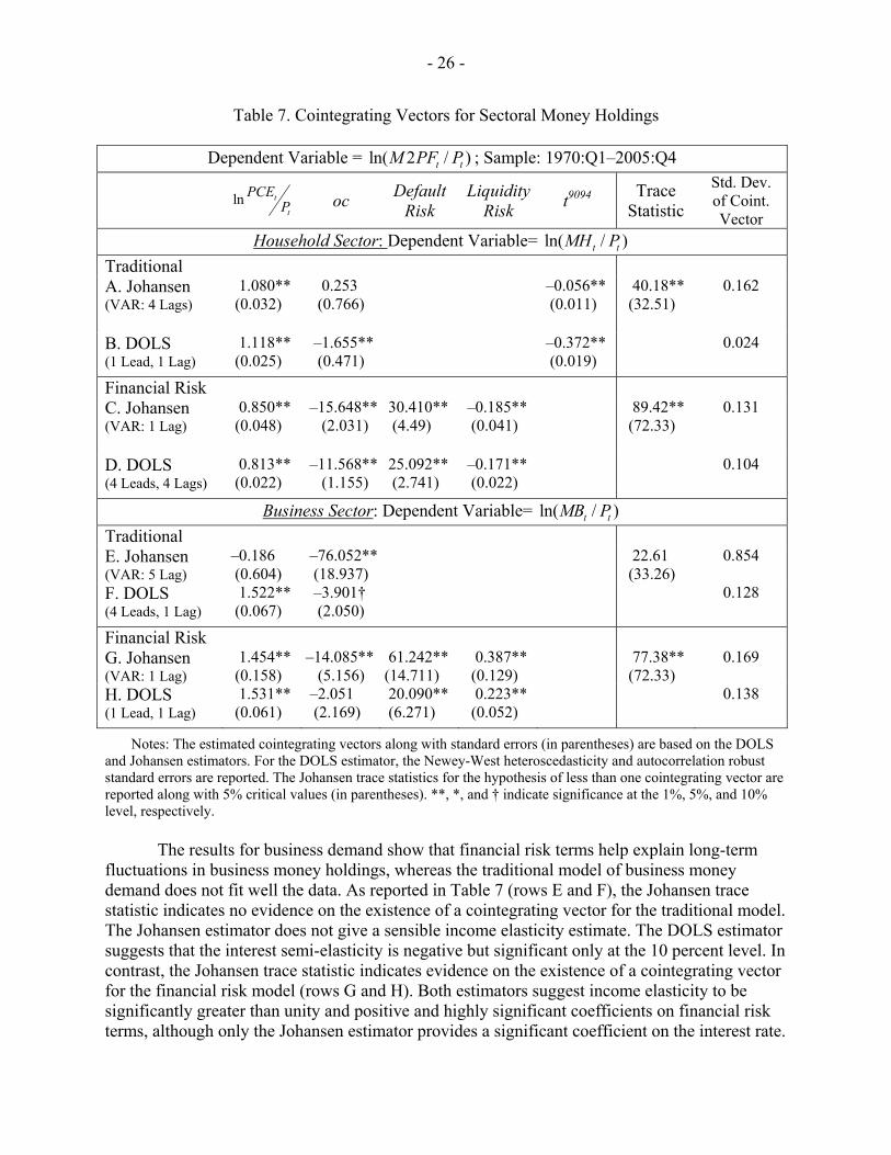
Household money demand becomes stable after accounting for the decline in financial trading costs in the early 1990s but is associated with financial risk variables less than expected. In Table 7, rows A and B report the results for the traditional model of household money demand with the t9094 term. The Johansen trace statistic suggests the existence of a cointegrating vector. In both the Johansen and DOLS estimators, the income elasticity is near but significantly greater than unity. The interest semi-elasticity is insignificant in the Johansen estimator but negative and significant in the DOLS estimator. As implied by the coefficient of t9094, the reduced financial trading costs lead to a substantial decrease in household money holdings, especially according to the DOLS estimator. That household money demand becomes stable after accounting for the decline in financial trading costs is perhaps not surprising given that the velocity of household money rises sharply in the early 1990s and stays roughly stable thereafter. The standard deviation of the cointegrating vector with the DOLS estimator is small, below 0.03. Apparently, the results of Carlson and others (2000) continue to hold for household money holdings. The financial risk model appears to be less valid for household money demand than for aggregate money demand. As shown in rows C and D, the Johansen trace statistic suggests the existence of a cointegrating vector, and the coefficient estimates from the Johansen and the DOLS estimators are qualitatively similar. The income elasticity is significantly lower than unity, and the interest semi-elasticity is negative and highly significant. The coefficient on Default Risk is positive and significant. However, the coefficient on Liquidity Risk is negative and significant. Also, the deviations from the DOLS cointegrating vector for the financial risk model are larger than those for the traditional model. Hence, the traditional model with t9094 may be quite valid for household money demand.

To explain a dramatic increase in money holdings by the business sector during the late 1990s, we consider the financial risk model of business money demand:

0 1 2 3 4ln lnt tt t t t

t t

MB BSO oc Default Risk Liquidity RiskP P

β β β β β ω= + ⋅ + ⋅ + ⋅ + ⋅ + , (7)

where BSO is the index of real business sector output calculated by the Bureau of Labor Statistics (available at the St. Louis Fed FRED II database) and Pt is the associated deflator. This model embeds the traditional model by setting 3 4 0β β= = . The traditional model does not include the t9094 term because there is no indication that business money demand permanently declines owing to a decline in investment costs in the early 1990s (while including the t9094 term has little effect on the results).

- 26 -

Table 7. Cointegrating Vectors for Sectoral Money Holdings

Dependent Variable = ln( 2 / )t tM PF P ; Sample: 1970:Q1–2005:Q4

ln t

t

PCEP

oc Default Risk

LiquidityRisk t9094 Trace

Statistic

Std. Dev. of Coint. Vector

Household Sector: Dependent Variable= ln( / )t tMH P Traditional A. Johansen (VAR: 4 Lags)

1.080** (0.032)

0.253 (0.766)

–0.056** (0.011)

40.18** (32.51)

0.162

B. DOLS (1 Lead, 1 Lag)

1.118** (0.025)

–1.655** (0.471)

–0.372** (0.019)

0.024

Financial Risk C. Johansen (VAR: 1 Lag)

0.850** (0.048)

–15.648** (2.031)

30.410** (4.49)

–0.185** (0.041)

89.42** (72.33)

0.131

D. DOLS (4 Leads, 4 Lags)

0.813** (0.022)

–11.568** (1.155)

25.092** (2.741)

–0.171** (0.022)

0.104

Business Sector: Dependent Variable= ln( / )t tMB P Traditional E. Johansen (VAR: 5 Lag)

–0.186 (0.604)

–76.052** (18.937)

22.61 (33.26)

0.854

F. DOLS (4 Leads, 1 Lag)

1.522** (0.067)

–3.901† (2.050)

0.128

Financial Risk G. Johansen (VAR: 1 Lag)

1.454** (0.158)

–14.085** (5.156)

61.242** (14.711)

0.387** (0.129)

77.38** (72.33)

0.169

H. DOLS (1 Lead, 1 Lag)

1.531** (0.061)

–2.051 (2.169)

20.090** (6.271)

0.223** (0.052)

0.138

Notes: The estimated cointegrating vectors along with standard errors (in parentheses) are based on the DOLS and Johansen estimators. For the DOLS estimator, the Newey-West heteroscedasticity and autocorrelation robust standard errors are reported. The Johansen trace statistics for the hypothesis of less than one cointegrating vector are reported along with 5% critical values (in parentheses). **, *, and † indicate significance at the 1%, 5%, and 10% level, respectively. The results for business demand show that financial risk terms help explain long-term fluctuations in business money holdings, whereas the traditional model of business money demand does not fit well the data. As reported in Table 7 (rows E and F), the Johansen trace statistic indicates no evidence on the existence of a cointegrating vector for the traditional model. The Johansen estimator does not give a sensible income elasticity estimate. The DOLS estimator suggests that the interest semi-elasticity is negative but significant only at the 10 percent level. In contrast, the Johansen trace statistic indicates evidence on the existence of a cointegrating vector for the financial risk model (rows G and H). Both estimators suggest income elasticity to be significantly greater than unity and positive and highly significant coefficients on financial risk terms, although only the Johansen estimator provides a significant coefficient on the interest rate.

- 27 -

B. Business Holdings of Quasi-Money

In the 1950s and 1960s, the vast majority of money held by the business sector was narrow money corresponding to M1. In the business sector, quasi-money holdings have grown faster than overall money holdings, and in recent years most money holdings were quasi-money. The velocity of quasi-money in the business sector has shown a secular downward trend, with the continued growth of quasi-money relative to output. As shown in Figure 7, business sector velocity fell relatively linearly over 1962–1997 except that a large velocity increase occurred in the late 1960s and early 1970s. The average growth rate of quasi-money holdings by business relative to business sector output before 1998 was greater than 4 percent per year. However, in the 1998–2002 period, money holdings increased by about 100 percent before leveling off.

We estimate the financial risk model of business quasi-money demand replacing

ln /t tMB P in equation (7) with ln /t tQMB P , where tQMB is business quasi-money. In this case, we use the AAA corporate yield rate rather than the Treasury-bill rate in measuring the opportunity cost, because firms would trade corporate debts for funding liquid assets.

Table 8 reports the estimated results of business demand for quasi-money for different

periods. The Johansen trace tests suggest the existence of a cointegrating vector for all periods. Several findings are noteworthy. First, the income elasticity tends to be significantly greater than unity. Second, the interest semi-elasticity is rather unstable and often insignificant, perhaps reflecting that returns on liquid assets, especially mutual funds, are highly correlated with market interest rates. Third, business money holdings are strongly associated with financial risk,

Figure 7. Velocity of Business Quasi-Money

-4.5

-4.0

-3.5

-3.0

-2.5

-2.0

-1.5

-1.0

-0.5

65 70 75 80 85 90 95 00 05

- 28 -

Table 8. Cointegrating Vectors for Business Quasi-Money Holdings

Dependent Variable = ln( / )t tMBQ P

ln t

t

BSOP

oc Default Risk

Liquidity Risk

Trace Statistic

Std. Dev. of Coint. Vector

Sample: 1970–2005 A. Johansen (VAR: 1 Lag)

2.961** (0.184)

–12.213* (5.517)

103.897** (14.777)

0.473** (0.107)

91.82** (72.33)

0.286

B. DOLS (1 Lead, 1 Lag)

2.863** (0.148)

–5.430 (4.664)

64.696** (10.929)

0.231** (0.07)

0.210

Sample: 1970–1995 C. Johansen (VAR: 1 Lag)

1.711** (0.181)

1.933 (3.995)

27.798** (9.805)

–0.181* (0.086)

116.12** (73.35)

0.273

D. DOLS (4 Leads, 4 Lags)

2.522** (0.284)

–3.705 (5.068)

56.370** (12.265)

0.074 (0.112)

0.216

Sample: 1970–1989 E. Johansen (VAR: 5 Lag)

0.671† (0.406)

–17.338† (11.210)

60.334** (23.337)

–0.599** (0.170)

105.62** (79.97)

0.504

F. DOLS (4 Leads, 1 Lag)

2.820** (0.314)

0.531 (5.874)

40.938** (11.065)

0.217** (0.125)

0.214

Notes: The estimated cointegrating vectors along with standard errors (in parentheses) are based on the DOLS and Johansen estimators. For the DOLS estimator, the Newey-West heteroscedasticity and autocorrelation robust standard errors are reported in parentheses. The Johansen trace statistics for the hypothesis of less than one cointegrating vector are reported along with 5% critical values (in parentheses). **, *, and † indicate significance at the 1%, 5%, and 10% level, respectively. especially for the whole period. The Default Risk coefficient is positive and strongly significant for both the Johansen and DOLS estimators. The Liquidity Risk coefficient is positive and significant for the whole period but rather mixed (negatively signed with the Johansen estimator) when the last 10-years are excluded in the sample period. This finding suggests that the liquidity risk factor emerged as an important factor in the recent decade: a strong surge in business quasi-money demand during 1998–2002 coincides with substantial increases in liquidity risk.

V. CONCLUSION

This paper examines empirically how changes in financial markets affect the holdings of monetary assets, considering that the expansion of new financial instruments such as mutual funds affects liquid asset allocation by households and businesses. We show that long-term fluctuations in financial market risk can explain the persistent fluctuations observed in broad money demand in the last 15 years. Money holdings increase with stock and bond market risks. However, the significant sensitivity of broad money demand to financial market risk indicators is a phenomenon that becomes relevant over the last 20 years. The financial market risk model fits the data much better in the last 20 years than it did before financial market deregulation.

- 29 -

We suggest two possible factors that may have increased the sensitivity of money demand to financial market risk. First, the cost of investing in stocks and bonds for ordinary savers has fallen, and holdings of bond and stock market mutual funds have become more prevalent. Earlier studies have argued that this factor resulted in a secular change in broad money demand. We argue that broader holdings of monetary assets may also make money holdings more sensitive to risk in financial markets. Second, our examination of sectoral money demand suggests that reduced costs of investing in financial assets lead to a secular decline in household money holdings. By contrast, business holdings of quasi-money have been increasing rapidly and persistently over time, and are sensitive to measures of financial market risk. In the last 15 years, the share of the business sector in broad money holdings has substantially increased. Therefore, it may not be surprising that aggregate broad money has become more sensitive to financial market risk.

This paper suggests that accounting for the evolution of financial markets is conducive to

regaining the stability of broad money demand. To the extent that the information value of money demand in predicting future inflation retains, policymakers may need to pay attention to the implication of a persistent shift in financial risk for future inflation. As suggested by recent studies, the evolution of sectoral money demand or financial innovations can change the impacts of exogenous shocks on economic activity (see Cole and Ohanian 2002; and Dynan and others, 2006). Therefore, it will be interesting in future research to examine how money holdings, interacting with financial markets and financial innovations, respond to shocks to the economy and thus affect economic activity. Also, an analytical relationship between money demand and financial risk in a shifting environment of financial development can be examined by accounting for financial transactions cost and substitutions in broad portfolio of assets—for example, substitutions between money and equity when investors face liquidity risk (Lerner and Schoar, 2004)—in an optimization framework, a topic worthy of further investigation. Further, there remains the need for seeking better surrogates than a broken time trend or a time dummy for the shifting environment of financial development.

- 30 -

References Acharya, Viral V., and Lasse Heje Pedersen, 2005, “Asset Pricing with Liquidity Risk,” Journal of

Financial Economics, Vol. 77 (August), pp. 375–410. Amihud, Yakov, 2002, “Illiquidity and Stock Returns: Cross-Section and Time-Series Effects,” Journal

of Financial Markets, Vol. 5 (January), pp. 31–56. Amihud, Yakov, and Haim Mendelson, 1986, “Asset Pricing and the Bid-Ask Spread,” Journal of

Financial Economics, Vol. 17 (December), pp. 223−249. Anderson, Richard G., Barry Jones, and Travis Nesmith, 1997, “Introduction to the St. Louis Monetary

Services Index Project” Federal Reserve Bank of St. Louis Review, Vol. 79 (January-February), pp. 25–30.

Anderson, Richard G., 2003, “Retail Deposit Sweep Programs: Issue for Measurement, Modeling, and

Analysis,” Federal Reserve Bank of St. Louis, Working Paper 2003-026. Anderson, Richard G., and Robert H. Rasche, 2001, “Retail Sweep Programs and Bank Reserves, 1994–

1999,” Federal Reserve Bank of St. Louis Review, (January/February), pp. 51–72. Besci, Zsolt, and Duca, John V., 1994, “Adding Bond Funds to M2 in the P-Star Model of Inflation,”

Economics Letters, Vol. 46 (October), pp. 143–147. Board of Governors of the Federal Reserve System, 2002, Monetary Policy Report to the Congress, pp.

1–32 (Washington: Board of Governors of the Federal Reserve System). Carlson, John B., Dennis L. Hoffman, Benjamin D. Keen, and Robert H. Rasche, 2000, “Results of a

Study of the Stability of Cointegrating Relations Comprised of Broad Monetary Aggregates,” Journal of Monetary Economics, Vol. 46 (October), pp. 345–383.

Carlson, John B., and Benjamin D. Keen, 1996, “MZM: A Monetary Aggregate for the 1990s?” Federal

Reserve Bank of Cleveland Economic Review, Vol. 32 (Second Quarter), pp. 15–23. Carlson, John B., and Jeffrey C. Schwarz, 1999, “Effects of Movements in Equities Prices on M2

Demand,” Federal Reserve Bank of Cleveland Economic Review, Vol. 35 (Fourth Quarter), pp. 2–9.

Carpenter, Seth B., and Joe Lange, 2003, “Money Demand and Equity Markets,” Finance and Economics Discussion Series 2003-3 (Washington: Board of Governors of the Federal Reserve System).

Choi, Woon Gyu, and David Cook, 2006, “Stock Market Liquidity and the Macroeconomy: Evidence from Japan,” Monetary Policy with Very Low Inflation in the Pacific Rim, NBER East Asia Seminar on Economics, Vol. 15, (edited by) Takatoshi Ito and Andrew Rose, pp. 309–336.

Choi, Woon Gyu, and Seonghwan Oh, 2003, “A Money Demand Function with Output Uncertainty, Monetary Uncertainty, and Financial Innovations,” Journal of Money, Credit, and Banking, Vol. 35 (October), pp. 685–709.

- 31 -

Chordia, Tarun, Richard Roll, and Avanidhar Subrahmanyam, 2000, “Commonality in Liquidity,” Journal of Financial Economics, Vol. 56 (April), pp. 3–28.

Cheung, Yin-Wong, and Kon S. Lai, 1993, “Finite-Sample Sizes of Johansen’s Likelihood Ratio Test for

Cointegration,” Oxford Bulletin of Economics and Statistics, Vol. 55 (August), pp. 313–328. Cochrane, John H., 2001, Asset Pricing, (Princeton and Oxford: Princeton University Press). Cole, Harold L., and Lee E. Ohanian, 2002, “Shrinking Money: The Demand for Money and the

Nonneutrality of Money,” Journal of Monetary Economics, Vol. 49 (May), pp. 653–686. Collins, Sean S., and Cheryl L. Edwards, 1994, “An Alternative Monetary Aggregate: M2 Plus

Household Holdings of Bond and Equity Mutual Funds,” Federal Reserve Bank of St. Louis Review, Vol.76 (November/December), pp. 7–30.

Dotsey, Michael , and Andreas Hornstein, 2003, “Should a Monetary Policymaker Look at Money?”

Journal of Monetary Economics, Vol. 50 (April) pp. 547–79. Dow Jr., James P., and Douglas W. Elmendorf, 1998, “The Effect of Stock Prices on the Demand for

Money Market Mutual Funds,” Finance and Economics Discussion Series 98-24 (Washington: Board of Governors of the Federal Reserve System).

Duca, John V., and David D. VanHoose, 2004, “Recent Developments in Understanding the Demand for

Money,” Journal of Economics and Business, Vol. 56 (July-August), pp. 247–272.

Duca, John V., 2003, “Stock Market Shocks and Broad Money Growth,” Manuscript, Federal Reserve Bank of Dallas.

Duca, John V., 2000, “Financial Technology Shocks and the Case of the Missing M2,” Journal of Money,

Credit, and Banking, Vol. 32 (November), pp. 820–839. Duca, John V., 1995, “Should Bond Funds Be Included in M2?” Journal of Banking and Finance, Vol. 19

(April), pp. 131–152. Duca, John V., 1994, “Would the Addition of Bond or Equity Funds Make M2 a Better Predictor of

Nominal GDP?” Federal Reserve Bank of Dallas Economic Review (Fourth Quarter), pp. 1–13. Duca, John V., 1993, “RTC Activity and the ‘Missing M2’. Economics Letters, Vol. 41 (n1), pp. 67–71. Duca, John V., 1992, “The Case of the Missing M2,” Federal Reserve Bank of Dallas Economic Review

(Second Quarter), pp. 1–19.

Duffee, Gregory R., 1998, “The Relation between Treasury Yields and Corporate Bond Yield Spreads,” Journal of Finance, Vol. 53 (December), pp. 2225–2241.

Dutkowsky, Donald H., and Cynamon, Barry Z., 2003, “Sweep Programs: The Fall of M1 and Rebirth of the Medium of Exchange,” Journal of Money, Credit, and Banking, Vol. 35 (April), pp. 263–279.

- 32 -

Dynan, Karen E. , Douglas W. Elmendorf, and Daniel E. Sichel, 2006, “Can Financial Innovation Help to Explain the Reduced Volatility of Economic Activity?” Journal of Monetary Economics, Vol. 53 (January), pp. 123–150

Fama, Eugene F., and Kenneth R. French, 1988, “Dividend Yields and Expected Stock Returns,” Journal of Financial Economics, Vol. 22 (October), pp. 3–26.

Feinman, Joshua, and Richard D. Porter, 1992. “The Continued Weakness in M2,” Finance and

Economics Discussion Series no. 209 (Washington: Board of Governors of the Federal Reserve System).

Federal Reserve Board, 2004, “Monetary Policy Report to the Congress,” Federal Reserve Bulletin

(spring), pp.125–152. Friedman, Milton, and Anna J. Schwartz, 1982, Monetary Trends in the United States and the United

Kingdom (Chicago: University of Chicago Press for the National Bureau of Economic Research). Fujimoto, Akiko, 2003, “Macroeconomic Sources of Systematic Liquidity,” Manuscript, Yale University. Gilbert, R. Alton, and A. Steven Holland, 1984, “Has the Deregulation of Deposit Interest Rates Raised

Mortgage Rates?” Federal Reserve Bank of St. Louis Review, Vol. 66 (May), pp. 5–15. Greber, Claus, and Wolfgang Lemke, 2005, “Money Demand and Macroeconomic Uncertainty,”

Deutsche Bundesbank Discussion Paper 26 (Frankfurt: Deutsche Bundesbank). Guerron, Pablo, 2006, “Time-Dependent Portfolio Adjustment: Yet Another Look at the Dynamics,”

Working Paper Series 006, Department of Economics, North Carolina State University. Hallman, Jeffrey J., Richard D. Porter, and David H. Small, 1991, “Is the Price Level Tied to the M2

Monetary Aggregate in the Long Run?” American Economic Review, Vol. 81 (September), pp. 841–858.

Hansen, Bruce E. 1997, “Approximate Asymptotic P Values for Structural-Change Tests.” Journal of

Business and Economic Statistics, Vol. 15 (1997), pp. 60−57. Hafer, R.W., and Dennis W. Jansen, 1991, “The Demand for Money in the United States: Evidence from

Cointegration Tests,” Journal of Money, Credit, and Banking, Vol. 23 (May), pp. 155–168. Harvey, Campbell R., 1989, “Time-Varying Conditional Covariances in Tests of Asset Pricing Models,”

Journal of Financial Economics, Vol. 24 (October), pp. 289–317. Hasbrouck, Joel, 2006, “Trading Costs and Returns for US Equities: Estimating Effective Costs from

Daily Data,” Mimeo. New York University. Jagannathan, Ravi, and Zhenyu Wang, 1996, “The Conditional CAPM and the Cross-Section of Expected

Returns” Journal of Finance, Vol. 51 (March), pp. 3–53. Johansen, Soren, 1988, “Statistical Analysis of Cointegration Vectors,” Journal of Economic Dynamics

and Control, Vol. 12 (June/September), pp 231–254.

- 33 -

Leeper, Eric M., and Jennifer E. Roush, 2003, “Putting "M" Back in Monetary Policy,” Journal of Money, Credit, and Banking, Vol. 35 (Part 2, December), pp. 1217–56.

Lerner, Josh, and Antoinette Schoar, 2004, “The Illiquidity Puzzle: Theory and Evidence from Private

Equity,” Journal of Financial Economics, Vol. 72 (April), pp. 3–40. Lucas, Robert E., Jr., 2000, “Inflation and Welfare,” Econometrica, Vol. 68 (March), pp. 247−74. Meltzer, Allan H., 2001, “The Transmission Process,” In: Deutsche Bundesbank (ed.), The Monetary

Transmission Process: Recent Developments and Lessons for Europe. Palgrave, London, pp. 112–130.

Nelson, Edward, 2002, “Direct Effects of Base Money on Aggregate Demand: Theory and Evidence,”

Journal of Monetary Economics, Vol. 49 (May), pp. 687–708. Ng, Serena, and Pierre Perron, 2001, “Lag Length Selection and the Construction of Unit Root Tests of

Good Size and Power,” Econometrica, Vol. 69 (November), pp. 1519–1554. Orphanides, Athanasios, and Richard D. Porter, 2000, “P* Revisited: Money-Based Inflation Forecasts

with a Changing Equilibrium Velocity,” Journal of Economics and Business, Vol. 52 (January-April), pp. 87–100.

Orphanides, Athanasios, Brian Reid, and David H. Small, 1994, “The Empirical Properties of a Monetary

Aggregate That Adds Bond and Stock Funds to M2,” Federal Reserve Bank of St. Louis Review, pp. 31–52.

Pastor, Lubos, and Robert F. Stambaugh, 2003, “Liquidity Risk and Expected Stock Returns,” Journal of

Political Economy, Vol. 111 (June), pp. 642–685. Sadka, R., 2004, “Liquidity Risk and Asset Pricing,” Mimeo. Northwestern University. Saikkonnen, Pentti, 1992, “Estimation and Testing of Cointegrated Systems by an Autoregressive

Approximation,” Econometric Theory, Vol. 8 (March), pp. 1–27. Sriram, Subramanian S., 2001, “A Survey of Recent Empirical Money Demand Studies,” IMF Staff

Papers, Vol. 47 (September), pp. 334–65. Stock James H., and Mark W. Watson, 1993, “A Simple Estimator of Cointegrating Vectors in Higher

Order Integrated Systems,” Econometrica, Vol. 61 (July), pp. 783–820.