Financial Literacy and the Financial Crisis · Financial Literacy and the Financial Crisis Leora F...

NBER WORKING PAPER SERIES

FINANCIAL LITERACY AND THE FINANCIAL CRISIS

Leora F. KlapperAnnamaria LusardiGeorgios A. Panos

Working Paper 17930http://www.nber.org/papers/w17930

NATIONAL BUREAU OF ECONOMIC RESEARCH1050 Massachusetts Avenue

Cambridge, MA 02138March 2012

We thank Ed Al-Hussainy, Andrei Markov, David McKenzie, Martin Melecky, Sue Rutledge, BilalZia, and seminar participants at the ISNIE 2011 at Stanford University, the CEPR/Study Center Gerzensee2011 European Summer Symposium, the McDonough School of Business, Essex Business Schooland the University of Venice for very valuable comments and the World Bank Development ResearchGroup Research Support Budget for financial assistance. Teresa Molina and Douglas Randall providedoutstanding research assistance. This paper’s findings, interpretations and conclusions are entirelythose of the authors and do not necessarily represent the views or policies of the World Bank, theirExecutive Directors, the countries they represent or the National Bureau of Economic Research.

NBER working papers are circulated for discussion and comment purposes. They have not been peer-reviewed or been subject to the review by the NBER Board of Directors that accompanies officialNBER publications.

© 2012 by Leora F. Klapper, Annamaria Lusardi, and Georgios A. Panos. All rights reserved. Shortsections of text, not to exceed two paragraphs, may be quoted without explicit permission providedthat full credit, including © notice, is given to the source.

Financial Literacy and the Financial CrisisLeora F. Klapper, Annamaria Lusardi, and Georgios A. PanosNBER Working Paper No. 17930March 2012JEL No. D14

ABSTRACT

The ability of consumers to make informed financial decisions improves their ability to develop soundpersonal finance. This paper uses a panel dataset from Russia, an economy in which consumer loansgrew at an astounding rate - from about US$10 billion in 2003 to over US$170 billion in 2008 - toexamine the importance of financial literacy and its effects on behavior. The survey contains questionson financial literacy, consumer borrowing (formal and informal), saving and spending behavior. Thepaper studies both the financial consequences and the real consequences of financial illiteracy. Eventhough consumer borrowing increased very rapidly in Russia, the authors find that only 41% of respondentsdemonstrate understanding of the workings of interest compounding and only 46% can answer a simplequestion about inflation. Financial literacy is positively related to participation in financial marketsand negatively related to the use of informal sources of borrowing. Moreover, individuals with higherfinancial literacy are significantly more likely to report having greater availability of unspent incomeand higher spending capacity. The relationship between financial literacy and availability of unspentincome is higher during the financial crisis, suggesting that financial literacy may better equip individualsto deal with macroeconomic shocks.

Leora F. KlapperThe World Bank1818 H Street, NWWashington, DC [email protected]

Annamaria LusardiThe George Washington UniversitySchool of Business2201 G Street, NWDuques Hall, Suite 450EWashington, DC 20052and [email protected]

Georgios A. PanosUniversity of StirlingStirling Management SchoolRoom 3B79, Cottrell BuildingEconomics DivisionStirling, Scotland, FK9 4LAUnited [email protected]

2

1. Introduction

The 2008 financial crisis, characterized in part by mounting losses for individuals,

has generated interest in better understanding how to promote savvier saving and

borrowing behavior. The ability of individuals to make informed financial decisions is

critical to developing sound personal finance, which can contribute to more efficient

allocation of financial resources and to greater financial stability at both the micro and

macro level (see, e.g., Lusardi, 2008; Lusardi and Tufano, 2009a,b). Efforts to improve

financial literacy can also be an important component of efforts to increase saving rates

and lending to the poorest and most vulnerable consumers (Cole, Sampson and Zia,

2011).

Our paper extends the existing literature in a new direction, using a panel survey

of financial literacy administered to a nationally representative sample of over 1,000

Russian individuals prior to and during the 2008 financial crisis. Russia is a particularly

important country to study given the large increase in consumer credit it has recently

experienced: Consumer loans (excluding mortgages) in Russia grew at an astonishing

rate: from about US$ 10 billion in 2003 to over US$ 170 billion in 2008—accounting for

over 10% of GDP in 2008 versus less than 1% in 2003 (World Development Indicators,

2010). This is one of the few panel data sets on financial literacy, and with it we are able

to address some novel questions, such as What is the level of financial literacy in a

country without a legacy of consumer credit and financial education? Are there not only

financial but also real consequences of low financial literacy? Are lower levels of

financial literacy related to greater financial vulnerability during a crisis, i.e., are less

financially literate individuals less able to deal with financial crises?

3

Assessing the direction of causality between financial literacy and financial

decision making or consumption and saving behavior has been a challenge in previous

work, as financial literacy is potentially an endogenous variable. However, this

assessment in a country like Russia may suffer less from the endogeneity problem, as

financial markets are not well developed and there are few financial education programs

in place. In our empirical work we are able to address this problem by relying on

instrumental variables (IV) estimation and using a new set of instruments, i.e., the

number of newspapers and the number of universities across regions, to measure

exposure to financial information or to peers with higher financial knowledge.

Importantly, because we have a panel data set, we are also able to account for

unobservable variables, such as intelligence, ability, and interest in financial matters,

which can also affect the relationship between financial literacy and financial or real

outcomes.

We find that even though consumer borrowing increased very rapidly in Russia

between 2003 and 2008, only 41% of respondents in our sample have an understanding of

the workings of interest compounding and only 46% can answer a simple question about

inflation. Financial literacy is not only low in the general population, but is particularly

severe among specific groups, such as women, those with low income and low

educational attainment, and those living in rural areas. Most importantly, we find that

financial literacy in Russia is significantly related to the use of formal banking and

borrowing and negatively related to the use of informal borrowing. Financial literacy has

real as well as financial consequences: Even after accounting for many characteristics and

income, individuals with greater financial literacy are significantly more likely to report

4

having higher availability of unspent income and less likely to report having experienced

lower spending capacity. In addition, the relationship between financial literacy and

availability of unspent income is stronger in 2009 versus 2008, showing that financial

literacy may better equip individuals to deal with macroeconomic shocks.

Our findings suggest that rapid growth of consumer credit combined with low

levels of financial literacy—and the shock of the global financial crisis—might end up

being a dangerous mix. As Russia transitions quickly to a market-based banking system,

financial education and basic financial literacy are still lagging. Many young Russians

have parents who did not have experience with bank loans (i.e., they did not have an

opportunity to receive financial education at home)1 and did not receive formal financial

literacy courses in school (i.e., there is no curriculum requirement for financial education

in Russia). Furthermore, consumer debt was almost non-existent before 2001, so few

individuals are likely to have long personal banking relationships or experience with

formal debt contracts and other financial products. In the context of current events, this is

likely to be the first financial crisis that most Russians are experiencing as borrowers.

The paper is organized as follows: Section 2 reviews the existing literature on

financial literacy and its effects on financial decision-making; Section 3 reviews the

environment for consumer finance in Russia; Section 4 describes our data, variables, and

summary statistics; and Section 5 presents our empirical strategy and reports our results.

Section 6 concludes.

1 Although state banks existed in Soviet times, their main role was to serve state-owned enterprises. There were no credit-reporting bureaus and the availability of credit to private firms and individuals was limited (McMillan and Woodruff, 2002). For the correlation between financial literacy of the young and parental background, see Lusardi, Mitchell, and Curto (2010).

5

2. Review of existing literature

Many papers have documented a strong correlation between financial literacy and

a set of behaviors. Bernheim (1995, 1998) showed that most households lack basic

financial knowledge and cannot perform very simple calculations, and that the saving

behavior of many households is dominated by crude rules of thumb. Hilgert, Hogarth,

and Beverly (2003) find a strong link between financial literacy and day-to-day financial

management. Financial literacy has also been linked to a set of behaviors related to

saving, wealth, and portfolio choice. For example, several papers have shown that

individuals with greater numeracy and financial literacy are more likely to participate in

financial markets and to invest in stocks (Christelis, Jappelli, and Padula, 2010; Yoong,

2011; Almenberg and Dreber, 2001; Almenberg and Widmark, 2011; Van Rooij, Lusardi,

and Alessie, 2011). Moreover, more literate individuals are more likely to choose mutual

funds with lower fees (Hastings and Tejeda-Ashton, 2008; Hastings and Mitchell, 2011).

Similarly, Lusardi and Mitchell (2007a, 2011d) show that those who display high

levels of literacy are more likely to plan for retirement and, as a result, accumulate much

more wealth, a finding reproduced in many of the countries that are part of an

international comparison of financial literacy, which includes Russia (Lusardi and

Mitchell, 2011c). Financial literacy is found to affect not only the assets side but also the

liability side of households’ balance sheet. Moore (2003) was one of the first to report

that respondents with lower levels of financial literacy are more likely to have costly

mortgages. More recently, Gerardi, Goette, and Meier (2010) report that those with low

literacy are more likely to default on sub-prime mortgage or have problems with them.

Stango and Zinman (2009) find that those who are not able to correctly calculate interest

6

rates out of a stream of payments end up borrowing more and accumulating lower

amounts of wealth. Campbell (2006) shows that individuals with lower incomes and

lower education levels—characteristics that are strongly related to financial literacy—are

less likely to refinance their mortgages during a period of falling interest rates. Lusardi

and Tufano (2009a,b) report that individuals with lower levels of financial literacy tend to

transact in high-cost manners, incurring higher fees and using high-cost methods of

borrowing. The less knowledgeable also report that their debt loads are excessive or that

they are unable to judge their debt position. Similar findings are reported in the UK

(Disney and Gathergood, 2011).

In addition to greater susceptibility to fraud and abuse, lack of financial literacy

might lead to borrower behavior that increases financial fragility (i.e., greater loan

losses). Informed consumers may also exercise innovation-enhancing demand on the

financial sector and play an important monitoring role in the market that can help

improve transparency and honesty in financial institutions. Furthermore, financial

illiteracy appears to be particularly severe for key demographic groups: women; the less

educated; those with low income; ethnic minorities; and older respondents (e.g.,

Bernheim, 1995; Lusardi and Mitchell, 2007a, 2007b, 2008, 2011b; Lusardi and Tufano,

2009a,b; inter alia).

Correlation between financial literacy and behavior does not mean causation, and

it is important to establish a causal link. Nevertheless, obtaining an exogenous source of

variation in financial literacy has been challenging. For example, it may be the desire to

invest in stocks or plan for retirement that causes individuals to invest in financial literacy

rather than the other way around. There also may be some omitted variables, such as

7

ability or patience, that affect both financial literacy and financial behavior. One way

around this problem is to look at financial mistakes and assess whether they are

correlated with financial literacy, as it is harder to argue that the causality goes from

mistakes to financial literacy. Interestingly, Agarwal et al. (2009) show that financial

mistakes are prevalent among the young and the elderly, which are the groups that

display the lowest levels of financial knowledge. Calvet, Campbell, and Sodini (2007,

2009) examine data from Sweden and look at actions of investors that can be classified as

mistakes. They find that poorer, less educated, and immigrant households—demographic

characteristics that are strongly associated with low financial literacy—are more likely to

make financial mistakes.

Another strategy has been to rely on instrumental variable (IV) estimation.

Several instruments have been used. For example, Lusardi and Mitchell (2009, 2011d)

follow Bernheim and Garrett (2001) in using high school financial literacy mandates in

different states and time periods in the United States. Van Rooij, Lusardi, and Alessie

(2011) have used the financial literacy of others, such as siblings and parents. Behrman et

al. (2010) use data from the Chilean Social Protection Survey and a set of plausibly

exogenous instrumental variables that satisfy critical diagnostic tests to isolate the causal

effects of financial literacy on wealth. All these studies show that financial literacy is

positively associated with a set of financial outcomes. Moreover, the IV estimates

indicate even more potent effects of financial literacy than suggested by OLS models.

Financial literacy also appears to be correlated with economic development; for

instance, the percentage of individuals in the United States that correctly answered

questions on interest compounding and inflation was 72% versus 79% in the Netherlands,

8

52% in Indonesia, 46% in Russia, and 34% in rural India (Figure 1).2 These findings have

been supported in recent studies using randomized control trials to explore the causal

impact of financial literacy on financial outcomes. For instance, in Indonesia, a randomly

selected set of unbanked individuals were offered financial literacy training sessions,

which were found to increase the demand for banking services among those with low

initial levels of financial literacy and low levels of education (Cole et al., 2011).

[Insert Figure 1 about here]

3. The Russian Banking System

This paper focuses on Russia, an economy that grew at a brisk rate in the past

decade and experienced a very sharp increase in consumer borrowing, as will be

described below. This setting provides a unique opportunity to examine the importance

and effects of financial literacy.

The Russian economy grew, on average, by almost 7% annually from 2001 to

2009, while annual per capita income grew from US$ 2,101 in 2001 to US$ 8,676 in

2009, an increase of over 400% (Figure 2). This rapid increase in purchasing power was

associated with an increase in demand for consumer credit, particularly for the purchase

of household appliances and other durable goods (Presniakova, 2006).3 Within this same

time period, as mentioned earlier, consumer loans grew at a very fast rate, reaching US$

170 billion in 2008 (preceding a decline to about US$ 120 billion in 2009). This

accounted for about 10% of GDP in 2009 versus about 2% in 2003.

2 Lusardi and Mitchell (2011a) for the U.S. and Cole et al. (2011) for Indonesia and India. The figure for Russia is calculated by the authors. 3 It is possible that Russians are more comfortable borrowing for durable goods, as buying goods on installment was quite popular in Soviet times.

9

[Insert Figure 2 about here]

In aggregate, the Russian banking system grew at a rate of over 40% between

2003 and 2008, with almost a trillion US$ in assets in 2008. Yet, despite this recent

growth, the Russian banking system remains small by international standards; domestic

credit to the private sector was 41% of GDP in 2008, relative to other markets such as

Brazil (54%), India (49%), and China (104%). In addition, the proportion of household

loans as a percentage of GDP in 2007 is below 10%, lower than the rate in many

developing Eastern European states (15%) and developed Western European states

(above 50%) (Oxford Analytica, 2007b). Furthermore, in 2006, close to 60 million

Russians (42% of the population) were estimated to not be part of the formal banking

system (Rohland, 2008).

Banks in Russia generally face an unfavorable investment climate, as indicated by

Russia’s ranking of 123rd out of 181 countries in the World Bank’s Ease of Doing

Business ranking (where 1 indicates the most favorable business environment) (Doing

Business, 2011). In this measure, Russia is ranked 89th in “getting credit,” which takes

into account creditor protection and the credit information sharing infrastructure.

Within this weak business environment, there is concern that the tremendous

growth of credit will be associated with high rates of default, in particular if rapid growth

in consumer credit is combined with low levels of financial literacy among borrowers.

The share of bad consumer loans was a sizeable 12.25% in 2010 (Central Bank of Russia,

2011). It is within this rather unique context that our survey instrument was designed.

4. Data and Summary Statistics

10

We use a panel dataset of Russian individuals in May/June 2008 and in June

2009. The 2008 sample was designed to be nationally representative at the individual

level, and weighted by gender, age, education, 46 oblasts (i.e., administrative regions),

and 7 federal region4 for a total of 1,600 individuals interviewed face-to-face.5 This is one

of the very few panel surveys measuring financial literacy and other key variables over

time. In 2009, 22% of individuals from the original sample either no longer resided at the

same location or refused to answer the follow-up survey. However, analysis of the data

between the two years does not show evidence of significant selection bias across the

covariates used in the empirical work (available upon request).

These surveys collected information on individual levels of financial literacy (i.e.,

numeracy, knowledge of interest compounding, understanding of inflation), as well as

use of financial services (e.g., the use of bank accounts and formal credit). The dataset

also provides rich demographic and socioeconomic information, and measures of

financial vulnerability. The primary respondent was the household head, without an age

limit.

[Insert Table 1 about here]

4.1 Demographic Information

Table 1 provides summary statistics of the pooled sample (2008 and 2009). The

percentage of male respondents is 43.9%, consistent with national census averages

4 Since March 1, 2008, the Russian Federation consists of 83 federal subjects. Six types of federal subjects are distinguished: 21 republics, 9 krais, 46 oblasts, 2 federal cities, 1 autonomous oblast, and 4 autonomous okrugs. We exclude the North-Caucasian (Chechnya) district because civil unrest prohibited surveying. 5 Summary statistics by gender, age, and education (% with secondary degrees) are very similar to those found in the 2002 Russia Longitudinal Monitoring Survey (LSMS), as well as the 2002 Russian National Census. Relative to the census data, however, our survey appears to under-represent individuals in the highest income bracket. This is likely the result of difficulty gaining access to the highest income individuals, many of whom live in gated housing communities, in order to conduct face-to-face interviews.

11

(Russian National Census, 2002). The average age in the pooled sample is around 45.

Most individuals (66%) live in households with three or more individuals, and 28.2% of

individuals live in urban regions, defined as settlements with a population greater than

500,000.

With respect to employment, 52.5% are employees (both skilled and unskilled),

while 25.5% are retirees. The education level of individuals in our sample is relatively

high: only 8.4% of the sample has less than a secondary education, 29.9% completed

secondary school, and 61.8% completed a special vocational/ technical school or initiated

or completed their higher education, a characteristic that sets Russia apart from other

emerging markets and makes it a particularly useful country to study.

The survey asks individuals to report their personal and household monthly

income, but these values are missing for almost 30% of the sample, i.e., individuals who

refused to answer.6 For our main regressions in the next section we impute missing

income observations and include dummies for brackets of family income rather than

using income values.7

The survey also includes a self-reported measure of income shocks.8 Individuals

are asked, “Did you (your family) experience an unexpected significant reduction of your

6 In our sample, mean personal monthly income for 2008 is US$ 762 (US$ 2,345 median income), while average family monthly income is US$ 1,494 (US$ 12,500 median). This compares closely with official statistics for 2008 of average per capita monthly income of US$ 1,404. Source: Russian Federation Federal State Statistics Service: http://www.gks.ru/bgd/regl/b10_06/IssWWW.exe/Stg/1/17-01.htm 7 The imputation methodology is based on regressions of family income on federal regions, gender, age, education categories, and self-assessed economic classification groups. The corresponding figures for each of the quartiles of the imputed income distribution are the following: Bottom quartile (1st): monthly income < US$833; 2nd quartile: $833 ≤ monthly income < $1,433; 3rd quartile: $1,433 ≤ monthly income < $2,084; 4th quartile: monthly income ≥ $ 2,084. 8 This is a categorical variable: the first category is individuals who report that they do not have enough money, even for food (7%); the next category is individuals who report they can buy food, but cannot buy clothes (23%); the third category is individuals who report they can buy food and clothes, but not durable goods (e.g., a television or refrigerator) (52%); finally, individuals who report they can buy durable goods (16%).

12

income over the past 12 months,” and we define a dummy “Income shocks” for those

who answer yes to this question. The summary statistics in Table 1 show that 35.9% of

the sample reported the experience of a negative income shock during 2009, showing that

the crisis and associated decline in income affected a large share of the Russian

population.


4.2 Use of Formal and Informal Credit

Our next set of variables measures financial inclusion, which includes variables

related to respondent affiliation with financial institutions and borrowing behavior.9 Our

first variable is “Bank Account,” which indicates whether an individual uses a bank

account (which includes the use of debit cards). In Russia it is common practice for an

employer to provide employees with an account and associated debit card, so-called

salary or “plastic” cards, at a bank chosen by the employer, and salaries are paid to these

accounts only. However, the employee can use this account only to withdraw salary, and

cannot make deposits to the account; thus, this may overestimate the actual voluntary

“use” of bank accounts (Danske Bank, 2011). Similarly, accounts might be used only to

withdraw government transfers. In our sample, 33.8% of respondents report using a

checking account in 2008 and 35% in 2009, with only 13 individuals (1.2%) adding an

account in 2009 and no individuals closing an account (changes in financial usage

between the two years are shown in Table 2).

9 An important feature to note about Russia is the absolute lack of and relatively low levels of trust in the banking sector, which is potentially an important factor in explaining the low level of use of banking products. Remarkably, only 28% of surveyed individuals in Russia report confidence in banks, the second to lowest score in the region (EBRD, 2006).

13

We also have information on consumer credit received from a bank or other

formal financial institution, including consumer debt, credit card debt, and mortgages.10

In 2008, 18.1% of our sample received bank credit and in 2009, 17.7% did so. Table 2

shows that 12.2% of the sample (131 individuals) used bank credit in 2008 but not in

2009, while 11.8% of the sample (127 individuals) who did not have bank credit in 2008

did have it in 2009.

We measure the use of informal debt by defining a dummy that equals one when

individuals respond “yes” to the question “Do you currently have debt?” but do not

report having any bank credit. In 2008, 17% of individuals in the sample report using

informal sources of borrowing, while 12.9% of individuals used informal borrowing in

2009; 13% of the sample used informal borrowing only in 2008, and 9% used informal

borrowing only in 2009. Note that informal borrowing typically involves shorter

repayment periods than formal borrowing, along with higher interest rates, penalties, and

other fees.

4.3 Capacity to Spend and Save

The next set of variables assesses respondent spending and saving capacity. The

survey includes a self-reported measure of spending capacity. This is a categorical

variable: the first category is individuals who report that they do not have enough money,

even for food (7%); the next category is individuals who report that they can buy food,

but cannot buy clothes (23%); the third category is individuals who report they can buy

food and clothes but not durable goods (e.g., a TV set or refrigerator) (52%); the final

category is individuals who report they can buy food, clothes, and durable goods (16%). 10 Less than 5% of individuals have a mortgage or credit card.

14

We use an ordinal variable ranking between 1 (highest spending capacity) and 5 (lowest

spending capacity) (see footnote 5) and, for robustness, define a dummy variable for

individuals who report not having enough money for more than food. As shown in Table

1, 31.6% of individuals in the sample report low spending capacity, with the figure being

higher during 2009 (33.1%, compared to 30.1% in 2008), consistent with the financial

crisis experienced in that time period.

A second set of variables measures the availability of unspent income, based on

the question “How often during the last 12 months did you (or your family) have any

money unspent from previous earnings before new revenues arrived.” The menu of

responses is “always,” “very often,” “sometimes,” “very rarely,” and “never.” Our main

results use an ordinal variable ranging from 1 to 5, and, for robustness, we also define a

dummy variable equal to one if the respondent reports “always” or “very often.” The

statistics shown in Tables 1 and 2 indicate that 39.4% of the sample report having

unspent income “always” or “very often” on a typical basis, and that the availability of

unspent income increased significantly from 34% in 2008 to 44.8% in 2009. We

speculate that at the onset of the crisis, some individuals increased their saving (and/or

reduced their spending), expecting to have lower income in the future. The ordinal

variable for the availability of unspent income has an average value of 2.36, with the

average being significantly higher in 2009 (2.57, compared to 2.14 in 2008).

4.4 Financial Literacy

15

Our survey includes four financial literacy questions, covering the concepts of

interest (two questions), inflation (one question), and sales discounts (one question). The

exact wording of the questions is reported below:

1) Let’s assume that you deposited 100,000 rubles in a bank account for 5 years at 10% interest rate. The interest will be earned at the end of each year and will be added to the principal. How much money will you have in your account in 5 years if you do not withdraw either the principal or the interest?

More than 150,000 rubles Exactly 150,000 rubles Less than 150,000 rubles I cannot estimate the amount even roughly

2) Let’s assume that you took a bank credit of 10,000 rubles to be paid back during a year in equal monthly payments. The credit charge is 600 rubles. Give a rough estimate of the annual interest rate on your credit. The interest rate is about:

3 % 6 % 9 % 12 % I cannot estimate it even roughly

3) Let’s assume that in 2010 your income is twice what it is now and that consumer prices also grow twofold. Do you think that in 2010 you will be able to buy more, less, or the same amount of goods and services as today?

More than today Exactly the same Less than today I cannot estimate it even roughly

4) Let’s assume that you saw a TV set of the same model on sale in two different shops. The initial retail price of it was 10,000 rubles. One shop offered a discount of 1,500 rubles, while the other one offered a 10% discount. Which one is a better bargain—a discount of 1,500 rubles or 10%?

A discount of 1,500 rubles A 10 % discount I cannot estimate it even roughly

Similar questions have been asked in other surveys, such as the U.S. Health and

Retirement Study, the American Life Panel, and the English Longitudinal Study on

Aging, and have been shown to measure both numeracy and financial knowledge

16

(Lusardi and Mitchell, 2009, 2011c; Banks and Oldfield, 2007; Stango and Zinman,

2009).

On average, in 2008, 41.4% of respondents correctly answered the question on

interest compounding; 23.3% correctly answered the monthly interest payment

calculation question; 45.6% correctly answered the question on inflation; and 69.5%

correctly answered the question on sales discounts. A large number of respondents

reported they “did not know” the answer to these questions. On average, in the pooled

sample, 30% of individuals replied “don’t know” to the question on interest

compounding; 49% to the question on monthly interest payments; 24% to the question on

inflation; and 22% to the question on sales discounts. These findings are similar to those

reported in other surveys (Van Rooij et al., 2011; Lusardi and Mitchell, 2011b; and

Lusardi and Tufano, 2009a,b), and in data in other seven countries (Lusardi and Mitchell,

2011c). Notably, we find that correct responses to all but one question increased during

the financial crisis, which might be explained by increased attention to financial issues in

the media or a rise in individuals’ interest in understanding their own finances.


4.4.1 Constructing a Financial Literacy Index

We construct an index of financial literacy using principal component analysis

(PCA) to summarize the information from the four questions detailed in the previous

subsection. For each question, we create a binary variable to identify the correct response

and perform PCA analysis based on polychoric correlations, following the method

developed to adapt PCA to ordinal data by Kolenikov and Angeles (2004). We estimate

17

the financial literacy index as the first principal component of the four financial literacy

questions. The procedure is described in greater detail in Appendix A for the year 2008

(the analysis for 2009 is available upon request). The corresponding distribution of

eigenvalues is presented in Appendix A, Panel B (the first component accounts for 53%

of the variation) and the factor loadings/scoring coefficients for the index are detailed in

Panel C.11 The financial literacy index distribution is shown in Panel E.

4.4.2 Who is Financially Literate in Russia?

Table 1, columns 2 and 3, show summary statistics for individuals with high and

low levels of financial literacy; asterisks indicate significant mean differences. We

identify “high” financial literacy as individuals with a financial literacy index greater than

the sample median. Univariate tests find that financially literate individuals are more

likely to be male, married or cohabiting, younger, and residents of urban Russian regions.

They are more likely to have vocational/technical, or some level of higher education, and

be employed in skilled or non-manual occupations. Importantly, individuals in the lowest

income quartile are more likely to score low in terms of their financial literacy, while

those in the highest income quartile are more likely to be highly financially literate. This

is consistent with many other surveys on financial literacy in other countries (see Lusardi

and Mitchell, 2011b, for an overview of financial literacy data in eight countries and

Christelis, Jappelli, and Padula, 2010, for an overview in eleven countries).

11 Although we retain the first factor for the purpose of parsimony, the optimal number of factors, identified by Humphrey-Ilgen parallel analysis (Lance, Butts, and Michels, 2006), is in fact two. We compare the number of factors derived from our survey data against factors for random numbers representing the same number of cases and variables and obtain the optimal number of factors at the intersection of plots of factors against cumulative eigenvalues for the two sets of data (Panel D).

18

Of primary interest to this study is the association between financial literacy and

financial outcomes. Table 1 indicates that there is a moderately positive association

between financial literacy and having a bank account (also shown in the correlation

matrix between financial literacy and bank account in Appendix Table B3). Individuals in

the high literacy group are also significantly more likely to use formal bank credit. In

addition, high literacy groups are significantly less likely to experience low spending

capacity, both in terms of the binary and the ordinal spending capacity variable. In

contrast, individuals with higher financial literacy are significantly more likely to

experience having unspent income and with higher frequency.

5. Financial and Real Consequences of Financial Literacy

The important question we aim to address in this paper is whether financial

literacy matters. To do so, we consider the following set of outcomes that expand upon

the previous literature. We first estimate a set of regressions in which the dependent

variable is (a) having a bank account, (b) using formal bank credit, and (c) using informal

credit. In addition to financial consequences we also look at real consequences. Our set of

dependent variables is (a) level of spending capacity and (b) availability of unspent

income. The sets of explanatory variables in our regressions include financial literacy,

gender, single-person household, the logarithm of age, a dummy for a negative income

shock during the last year, and dummy variables for education (4 dummies), occupation

(8 dummies), family income quartiles, and federal region of residence (7 dummies).

5.1 Empirical Strategy

19

Because we have a panel data set, we are better equipped to assess the effect of

financial literacy on a set of outcomes than previous studies. First, we use 2009 measures

of financial inclusion and outcomes and 2008 values of financial literacy and other

explanatory variables. We use past values of the independent variables to account for

both the potential simultaneity between financial literacy and financial outcomes, along

with the potential endogeneity of the financial literacy measure.

Second, we use IV estimation to assess the impact of financial literacy on

financial behavior. Two instruments are used: (a) the number of newspapers in circulation

per two-digit region (both regional and national) and (b) the total number of universities

per two-digit region (both public and private). The two variables can be expected to be

correlated with financial literacy in terms of “exposure” to newspaper readership (either

directly or through family members and neighbors who read the paper) and higher

education of peers in the region. The experience of others is not under the control of the

respondent and is thus exogenous with respect to his or her actions, but respondents can

learn from those around them, thus increasing their own literacy. Several other studies

have documented that individuals learn about financial matters from peers (Duflo and

Saez, 2003; Hong, Kubik, and Stein, 2004; and Brown, Ivkovic, Smith, and Weisbenner,

2008). Studies have also documented the importance of proximity to a university as an

exogenous measure of financial knowledge (Christiansen, Joensen, and Rangvid, 2008).

The bottom of Table 1 shows that the average number (by two-digit region) of

newspapers is 56 and the average number of universities is 18 (11 public and 7 private).

20

Appendix C presents maps illustrating the regional variation in the number of newspapers

in circulation and the number of universities in the 46 Russian oblasts of our sample.12

Third, to account for unobserved heterogeneity that can account for the

relationship between financial literacy and our set of outcomes, we use both years of data

and estimate individual random effects and fixed effects models.

5.2 Empirical estimates: Financial outcomes

Our first set of estimates examines the correlates of the use of bank accounts by

respondents in our sample. Due to the low number of new bank accounts for the year

2009 in the sample, panel models cannot be estimated. Table 4 presents probit estimates.

The dependent variable is a dummy equal to one if the individual reports having a bank

account in 2009 and equal to zero otherwise. Explanatory variables are dated as of 2008

in order to mitigate as much as possible simultaneity problems. Marginal effects and

robust standard errors are presented throughout the table.

Column 1 of Panel A shows the baseline probit estimates, which exclude

measures of financial literacy. We find that individuals who are older, more educated,

and have higher income are more likely to have a bank account, consistent with findings

in other countries (Christelis, Jappelli, and Padula, 2010; Cole, Sampson and Zia, 2011).

Columns 2, 3, and 4 include our two measures of financial literacy (an index and the

number of correct responses to the financial literacy questions). Both measures show a

significantly positive effect (at the 10% level) of financial literacy on the likelihood of

12 In terms of federal regions (figures available upon request), the Central federal region, Volga, and the Southern region have the highest newspaper circulation, while the Urals, the Far-Eastern, and the Siberian region have the lowest numbers of newspapers in circulation. Moreover, the Southern region has the highest number of universities, with the next highest being the North-Western and the Central regions. The lowest numbers of universities are found in the Urals, the Far-Eastern, and the Siberian federal region.

21

using a bank account. The marginal effects suggest a sizeable impact: a one standard

deviation increase from the average level of financial literacy raises the likelihood of

using a bank account by 6.3–8.8%, depending on the measure used. Also note that adding

financial literacy does not much affect the estimates of education; thus, financial

knowledge has an effect above and beyond general schooling.


Panel B of Table 4 presents IV probit estimates of the probability of using a bank

account. In this specification, we take into account that financial literacy could be an

endogenous variable. Moreover, financial literacy can be measured with error, and this

can also affect the estimated effect of financial literacy on the probability of having a

bank account. As discussed earlier, the set of instruments used to instrument financial

literacy is the total number of newspapers in circulation and the number of public and

private universities in every Russian oblast. The first-stage regressions are shown in

Appendix Table B1. The two instruments have a positive and statistically significant

impact on financial literacy. Both the F-statistics from the tests of joint significance and

the LM tests of omitted variables shown at the bottom of the table reject the null

hypotheses of joint insignificance and “significant improvement” to the model.13

The estimates in the second stage, reported in the last two columns of Table 4,

show that the relationship between literacy and bank account ownership remains positive,

statistically significant, and is somewhat larger in the IV probit estimates than in the OLS

estimates. Moreover, the exogeneity test is not rejected. Thus, the OLS estimates do not

13 The tests stem from two separate specifications for the first stage models, i.e. one incorporating the two instruments and another without the two instrumental variables, respectively.

22

differ significantly from the IV estimates. Moreover, the Hansen J statistic of

overidentifying restriction at the bottom of the table shows that the instruments are valid.

In Table 5, we examine the impact of financial literacy on the probability of using

formal bank credit. The probit estimates with past values (dated 2008) of the independent

variables in Columns A2 and A3 show that financial literacy is significantly positively

related to the likelihood of having formal credit. The marginal effects show that a one

standard deviation increase from the average level of financial literacy raises the

likelihood of acquiring formal credit by 14–18%, depending on the measure used.


Panel B of Table 5 presents IV probit estimates. The statistics reported at the

bottom of the table reject the hypothesis that the instruments are not valid.14 The

estimates confirm the positive and statistically significant association between financial

literacy and formal credit. The magnitude of the marginal effects is very similar to the

baseline probit estimates.

One concern is that there are omitted variables (for example, ability) that can bias

the estimated effect of financial literacy. In Panels C and D of Table 5 we make use of the

panel aspect of the data and report estimates from random effects probit and fixed effects

logit models. The latter model excludes observations that do not vary within the panel,15

and hence uses a smaller sample. Both the marginal effects from the random effects

14 Additional linear probability models examine instrument validity. The results are available upon request. The weak-instrument robust-inference tests examine the null hypothesis that the coefficients of the endogenous regressors in the structural equation are jointly equal to zero and that the overidentifying restrictions are not rejected. Both tests are robust to the use of weak instruments. The tests are equivalent to estimating the reduced form of the equation (with the full set of instruments as regressors) and testing that the coefficients of the excluded instruments are jointly equal to zero. The Hansen J statistic of overidentifying restriction at the bottom of the table marginally rejects the null hypothesis that the instruments are valid at the 10% level. 15 Moreover, we exclude age in the fixed effects model to achieve identification.

23

model and the odds ratios for the fixed effects model confirm the positive association

between financial literacy and bank credit. Hence, an increase in the financial literacy

score within the year is associated with a higher likelihood of acquiring formal credit.

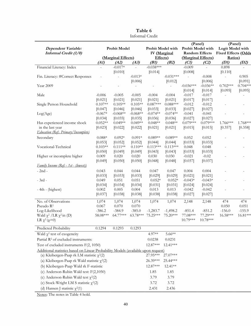
Finally, Table 6 examines the likelihood of using informal credit as the dependent

variable. The marginal effects from the probit model with past values of the independent

variables, shown in Column 1, suggest that single individuals (those living in single

person households) and those with low educational attainment are more likely to use

informal credit. Moreover, individuals who experienced a negative income shock during

the last year are more likely to use informal credit, which provides some evidence as to

how Russians have dealt with shocks. Columns A2 and A3 add financial literacy

measures, i.e., the index and the number of correct responses, respectively. Financial

literacy is negatively associated with the likelihood of using informal credit. The

marginal effects suggest that a one standard deviation increase from the average level of

financial literacy reduces the likelihood of acquiring formal credit by 10–13%, depending

on the measure used and given the overall predicted probability of the model. The effects

are statistically significant at the 1% level.


Panel B presents the marginal effects and robust standard errors from the IV

probit regressions using the same instruments that were mentioned previously. The tests

at the bottom of the table confirm the validity of the instruments. The results confirm the

negative association seen previously between financial literacy and use of informal credit.

The magnitude of the coefficient estimates increased by almost twofold compared to the

24

simple probit model estimates, and the coefficient becomes statistically significant at the

1% level.

The models in Panels C and D indicate weaker negative associations between

financial literacy and informal credit, and the negative effects shown are not significant at

any conventional levels. Interestingly, the significance of the year 2009 crisis dummy and

income shock dummy in the fixed effects model appear to highlight the use of informal

credit as a primary way to deal with shocks.

5.3 Real effects of financial literacy

We turn now to the real consequences of financial literacy. In this section, we

examine the relationship between financial literacy and financial vulnerability indicators,

such as respondent level of spending capacity and availability of unspent income. Tables

7 and 8 replicate the same four sets of estimates as the previous tables, using as

dependent variables (a) an ordinal spending capacity variable, ranging from 1 (high

spending) to 5 (low spending), and (b) an ordinal variable capturing the availability of

unspent income, ranging from 1 (low frequency) to 5 (high frequency).

The results in Table 7 show that older individuals, as well as those in the lowest

income quartiles, are more likely to experience low spending capacity. The addition of

the financial literacy variables in the ordered probit models of Columns A2 and A3

indicates that financial literacy also matters for spending; those who are more financially

literate are less likely to report low spending capacity during the financial crisis. The IV

estimates in Panel B continue to confirm the negative association between financial

literacy and low spending capacity.

25


Moreover, the panel models in Panels C and D of Table 7 confirm the negative

relationship between financial literacy and low spending capacity, both in the random

effects GLS model and within groups, in the fixed effects model. The results are

statistically significant at all conventional levels, and the magnitude of the effects is

similar to those of the previous model. In the panel models of Table 7, two additional

specifications are introduced in Columns C2 and D2.16 These include interaction terms

between financial literacy variables and the dummy variable for the year 2009. The

rationale for adding those variables is to examine whether the interaction between

financial literacy and the year of the financial crisis is significantly associated with lower

spending capacity. However, both sets of interaction terms are not statistically significant.


In Table 8, we use the frequency of having unspent income as (an ordinal)

dependent variable and present estimates of ordered probit models and linear models for

two-stage least squares, random effects GLS, and fixed effects in Panels A, B, C, and D,

respectively. The model’s first three rows show a significantly positive coefficient of

financial literacy on the availability of unspent income. The baseline ordered probit

estimates in Column 1 show that males and high-income individuals are more likely to

have income that is unspent on a regular basis. Columns A2 and A3 add the financial

literacy variables to the ordered probit specification and show that financial literacy is

significantly positively related to the incidence of having unspent income available. The

16 These results are robust to the substitution of the financial literacy index with the number of correct responses, which are not shown.

26

finding is robust. The IV probit estimates in Panel B confirm a significant and positive

effect of financial literacy.17

Moreover, the estimates from random effects GLS models in Panel C show a

positive effect of financial literacy in the panel sample, with marginal effects similar in

magnitude to those of the probit model. The inclusion of the interaction terms between

financial literacy and the year 2009 in the panel models shows a significant positive

interaction term. Thus, financially literate individuals are significantly more likely to

have unspent income in the year 2009. Moreover, the fixed effects model in Panel D

shows a positive interaction term for the effect of financial literacy. This suggests that

more literate individuals in 2009 are more likely to save more frequently, as compared to

less literate individuals.

5.4 Robustness exercises

In Appendix Tables B2–B4 we perform three sets of robustness exercises to check

the validity of our findings. The estimates in Table B2 in the Appendix replicate the level

of spending estimates, using a binary variable for low spending as the dependent variable.

All four panels of Table B2 exhibit statistically significant negative coefficients of the

financial literacy measures on spending. In the panel models, the interaction terms

between financial literacy and the year 2009 are negative, but once again statistically

insignificant. The magnitude of the marginal effects in the probit model of Panel A is

such that a one standard deviation from the average level of financial literacy reduces the

likelihood of experiencing low levels of spending capacity by 8.5–10%, depending on the

17 Similarly, Klapper and Panos (2011) find that financial literacy is positively related to participating in private and public retirement plans and negatively related to informal ways of saving for retirement.

27

measure used and given the overall predicted probability of the model. The IV probit

estimates in Panel B confirm the negative association between financial literacy and low

spending, along with the validity of the instruments used. The magnitude of the

coefficients in the IV model is very similar to the probit model. Moreover, the sign and

statistical significance (10% level) of financial literacy is the same, which suggests that

the instruments used are valid.

Appendix Table B3 presents estimates for models with a binary version of

unspent income as the dependent variable. Columns A2 and A3 show that financial

literacy is significantly positively related to the incidence of having unspent income. The

magnitude of the marginal effects presented suggests that a one standard deviation

increase in financial literacy raises the likelihood of having unspent income by 10–

11.5%. The IV probit estimates in Panel B confirm this. They show a significant positive

marginal effect of financial literacy, of a slightly lower magnitude than the probit model,

and also confirm the validity of the instruments used. Moreover, the estimates from

random effects probit models in Panel C show a positive effect of financial literacy in the

panel sample, with marginal effects similar in magnitude to those of the probit model.

The inclusion of the interaction terms between financial literacy and the year 2009 in the

panel models shows a significant positive interaction term. Hence, financially literate

individuals are significantly more likely to have unspent income available in the year

2009. However, the fixed effects models in Panel D fail to show significance of the

financial literacy variables within individuals although the odds ratios obtained are

positive and greater than one.

28

Finally, in Appendix Table B4, we perform an additional robustness check

concerning the validity of our instruments. We use specifications similar to our IV

regressions in the previous tables, but also include control variables for the log values of

the regional unemployment rate and the average monthly income per capita in every

administrative region.18 These robustness checks largely refute that the impact of our

instrumental variables is due to regional differences in living standards. All financial

literacy effects remain large and statistically significant, with the only exception being the

effects in the spending regressions, where the coefficients become smaller in magnitude

and statistically insignificant. This is indeed the variable that is likely to be affected the

most by regional living standard differences. Hence, the results confirm the robustness of

our instruments, and the magnitude of the majority of the effects remains high and

statistically significant.

In unreported regressions, we use self-assessed financial literacy (on a scale from 1

to 5) in place of the financial literacy measures used so far. Our results prove robust to

the use of this measure and are available upon request.

6. Conclusion

Our study contributes to the literature on financial literacy by examining its

effects on both financial and real behavior in a relatively understudied context, that of an

emerging market experiencing a financial crisis. We find that financial literacy is

significantly related to greater participation in formal financial markets and negatively

related to the use of informal sources of borrowing. Moreover, individuals with higher

18 The data is available from the Russian Federation Federal State Statistics service at: http://www.gks.ru/bgd/regl/b10_06/IssWWW.exe/Stg/1/17-01.htm

29

levels of financial literacy are significantly more likely to report greater levels of unspent

income and less likely to report lower levels of spending. Finally, the relationship

between financial literacy and the level of unspent income is higher during the financial

crisis, after controlling for household characteristics. Our results suggest that greater

financial literacy can help individuals face unexpected macroeconomic and income

shocks.

30

References Agarwal, S., J. Driscoll, X. Gabaix, and D. Laibson (2009). The age of reason: Financial

decisions over the lifecycle with implications for regulation, Brookings Papers on Economic Activity, Fall 2009, 51–101.

Almenberg, J., and A. Dreber (2011). Gender, financial literacy and stock market

participation. Working Paper, Stockholm School of Economics. Almenberg, J., and J. Widmark (2011). Numeracy, financial literacy and participation in

asset markets. Mimeo, Swedish Ministry of Finance. Anderson, J.A. (1984). Regression and Ordered Categorical Variables. Journal of the

Royal Statistical Society Series B 46:1, 1–30. Banks, J., and Z. Oldfield (2007). Understanding pensions: Cognitive functions,

numerical ability and retirement saving. Fiscal Studies 28(2): 143-170. Behrman, J., O. S. Mitchell, C. Soo, and D. Bravo (2010). Financial literacy, schooling,

and wealth accumulation. NBER WP 16452. Bernheim, D. (1995). Do households appreciate their financial vulnerabilities? An

analysis of actions, perceptions, and public policy, in: Tax Policy and Economic Growth, American Council for Capital Formation, Washington, DC, 1–30

Bernheim, D. (1998). Financial illiteracy, education and retirement saving. In O. Mitchell

and S. Schieber (eds.), Living with Defined Contribution Pensions, University of Pennsylvania Press, Philadelphia, 38–68.

Bernheim, D. and D.M. Garrett (2001). The effects of financial education in the

workplace: evidence from a survey of households. Journal of Public Economics 87(7-8), 1487–1519

Brown, J., Z. Ivkovic, P. Smith, and S. Weisbenner (2008). Neighbors matter: Causal

community effects and stock market participation. Journal of Finance 63, 1509–1531.

Calvet, L., J. Campbell, and P. Sodini. 2007. Down or out: Assessing the welfare costs of

household investment mistakes, Journal of Political Economy 115: 707–747 Calvet, L., J. Campbell, and P. Sodini (2009). Measuring the financial sophistication of

households. American Economic Review 99(2): 393–398. Campbell, J. (2006). Household Finance, Journal of Finance, 61, 1553–1604.

31

Central Bank of Russia (2011). Banking Supervisions Report, Moscow Christelis, D., T. Jappelli, and M. Padula (2010). “Cognitive Abilities and Portfolio

Choice”. European Economic Review 54, 18–38. Christiansen, C., J. Joensen and J. Rangvid. (2008). Are economists more likely to hold

stocks? Review of Finance 12, 465–496. Claudill, S. B. (2000). Pooling choices or categories in multinomial logit models.

Statistical Papers No. 41, pp. 353–358 Cole, S., T. Sampson, and B. Zia (2011). Prices or Knowledge? What Drives Demand for

Financial Services in Emerging Markets? Journal of Finance (66)6, 1933–1967. Danske Bank (2011). Business Guide Russia. Danske Bank: Copenhagan. Disney, R., and J. Gathergood (2011). Financial literacy and indebtedness: New evidence

for UK Consumers. Mimeo, University of Nottingham Doing Business (2011). Available on-line at: www.doingbusiness.org Duflo, E., and E. Saez (2003). The Role of Information and Social Interactions in

Retirement Plan Decisions: Evidence from a Randomized Experiment. Quarterly Journal of Economics. 118:3, 815–842.

EBRD (2006). Life in Transition Survey. European Bank for Reconstruction and

Development: United Kingdom. Gerardi, K., L. Goette, and S. Meier (2010). Financial literacy and subprime mortgage

delinquency: Evidence from a survey matched to administrative data. Federal Reserve Bank of Atlanta Working Paper 2010-10.

Hastings, J., and O. S. Mitchell (2011). How financial literacy and impatience shape

retirement wealth and investment behaviors. NBER Working Paper 16740. Hastings, J., and L. Tejeda-Ashton (2008). Financial Literacy, Information, and Demand

Elasticity: Survey and Experimental Evidence from Mexico. NBER Working Paper No. 14538

Hilgert, M., J. Hogarth, and S. Beverly (2003). Household Financial Management: The

Connection between Knowledge and Behavior, Federal Reserve Bulletin, 309–32. Hong, H., J. D. Kubik, and J. C. Stein (2004). Social Interaction and Stock-Market

Participation. The Journal of Finance 59(1), 137–163

32

Klapper, L., and G.A. Panos (2011). “Financial Literacy and Retirement Planning: the Russian Case.” Journal of Pension Economics and Finance 40, no 4, pp. 599–618.

Kolenikov, S., and G. Angeles (2004). The Use of Discrete Data in Principal Component

Analysis With Applications to Socio-Economic Indices. CPC/MEASURE Working paper No. WP-04-85.

Kolenikov, S., and G. Angeles (2008). Socioeconomic status measurement with discrete

proxy variables: Is principal component analysis a reliable answer? Working paper.

Lance, C., M. Butts, and L. Michels (2006). The sources of four commonly reported

cutoff criteria: What did they really say? Organizational Research Methods, No. 9, pp. 202-220.

Long, J.S., and J. Freese (2006). Regression Models for Categorical Dependent Variables

Using Stata (2nd Edition). StataCorp LP. Lusardi, A. (2008). Overcoming the Saving Slump: How to Increase the Effectiveness of

Financial Education and Saving Programs. University of Chicago Press. Lusardi, A. and O. S. Mitchell (2007a). Baby Boomer Retirement Security: The Role of

Planning, Financial Literacy, and Housing Wealth. Journal of Monetary Economics, 54, pp. 205–224

Lusardi, A., and O.S. Mitchell (2007b), Financial Literacy and Retirement Planning: New

Evidence from the Rand American Life Panel. MRRC Working Paper n. 2007-157.

Lusardi, A., and O. S. Mitchell (2008). Planning and Financial Literacy. How Do Women

Fare? American Economic Review, 98(2), pp. 413–417. Lusardi, A., and O. S. Mitchell (2009). How ordinary consumers make complex

economic decisions: Financial literacy and retirement readiness NBER Working Paper 15350.

Lusardi, A., and O. S. Mitchell (2011a). Financial Literacy and Planning: Implications for

Retirement Wellbeing, forthcoming in A. Lusardi and O. Mitchell (eds.), Financial Literacy: Implications for Retirement Security and the Financial Marketplace, Oxford University Press, 2011.

Lusardi, A., and O. S. Mitchell (2011b). Financial literacy around the world: an

overview. Journal of Pension Economics and Finance 10(4), pp.497–508.

33

Lusardi, A., and O. S. Mitchell (2011c). Financial literacy and retirement planning in the United States. Journal of Pension Economics and Finance 10(4), pp. 509–525.

Lusardi, A., and O. S. Mitchell. (2011d). Financial literacy and retirement planning in the

United States, forthcoming Journal of Pension Economics and Finance. Lusardi, A., O. S. Mitchell, and V. Curto. (2010). Financial literacy among the young,

Journal of Consumer Affairs 44 (2): 358–380. Lusardi, A., and P. Tufano (2009a). Debt Literacy, Financial Experiences and

Overindebtedness. NBER Working Paper n. 14808. Lusardi, A. and P. Tufano (2009b). Teach Workers about the Perils of Debt. Harvard

Business Review McMillan, J. and C. Woodruff (2002). The Central Role of Entrepreneurs in Transition

Economies. Journal of Economic Literature. 16:3, 153–170. Moore, D. (2003). Survey of Financial Literacy in Washington State: Knowledge,

Behavior, Attitudes, and Experiences. Technical Report n. 03-39. Social and Economic Sciences Research Center, Washington State University.

Oxford Analytica (2007b). RUSSIA: Consumer credit rises but problems persist. Global

Strategic Anlysis.08.10.2007 Presniakova, L. (2006). Consumer Credit. The Public Opinion Foundation Database.

June. Rohland, K. (2008). Russian Banking Sector Recent Progress and Challenges For the

Future. Banking Forum of the CIS Countries and Eastern Europe, Vienna, April 24–27.

Russia Longitudinal Monitoring Survey (2002). Available on-line at:

http://www.cpc.unc.edu/projects/rlms-hse Stango, V. and J. Zinman (2009). Exponential Growth Bias and Household Finance.

Journal of Finance 64. 2807–2849. Van Rooij, M., A. Lusardi, and R. Alessie (2011). Financial Literacy and Stock Market

Participation. Journal of Financial Economics. World Development Indicators (2011). Available on-line at: data.worldbank.org. Yoong, J. (2011). Financial illiteracy and stock market participation: Evidence from the

RAND American Life Panel. In Olivia S. Mitchell and Annamaria Lusardi. Financial Literacy: Implications for Retirement Security and the Financial Marketplace. Forthcoming, Oxford University Press.

35

Figure 1: Financial Literacy, % of individuals answering correctly

Source: Cole, et al. (2010); the authors; Cole, et al. (2010); Lusardi and Mitchell (2007a); van Rooij, et al. (2008), respectively.

Figure 2: Russian Household Debt (US$, billions) and Per Capita Income (US$)

1.7 3.3 4.6 9.7

21.3

42.0

76.4

124.5

173.8

121.3

0

2000

4000

6000

8000

10000

12000

‐

30

60

90

120

150

180

210

240

'00 '01 '02 '03 '04 '05 '06 '07 '08 '09

Household debt, US$, billions (left axis) GDP per capita, US$ (Right axis)

Source: WB-WDI Statistics (2010)

36

Table 1 Summary Statistics

Pooled Financial Literacy Index sample High (≥median) Low (<median)

#Obs. 2,148 986 1,162 Male 43.9% 46.7%** 41.5% Single Person Household 11.6% 8.7% 14.0%*** Age 45.13 41.36 48.33*** Urban region 28.2% 37.0% 35.0% Has experienced negative income shock in last year 35.9% 32.2%*** 24.9%

Education: Primary or Incomplete 8.4% 4.3% 11.9%*** Secondary 29.9% 26.3% 33.0%*** Vocational-Technical 38.4% 41.1%** 36.1% Higher or incomplete higher 23.4% 28.4%*** 19.1% Occupation: Skilled Non-Manual 9.0% 11.7%*** 6.8% Skilled Manual 26.9% 30.0%*** 24.3% Unskilled Non-Manual 13.5% 15.6%*** 11.7% Unskilled Manual 3.1% 3.0% 3.1% Entrepreneur 2.8% 3.1% 2.5% Unemployed 0.9% 0.8% 1.0% Pensioner 25.5% 15.5% 34.0%*** Other 18.3% 20.2%** 16.6%

Family Income 20,354.3 23,511.1*** 17,675.7 - 1st Quartile - (lowest) 26.3% 18.1% 33.2%*** - 2nd Quartile - 25.1% 25.3% 24.9% - 3rd Quartile - 23.1% 24.4% 22.0% - 4th Quartile - (highest) 25.6% 32.3%*** 19.9%

Federal region: Central 27.1% 27.9% 26.4% North-Western 10.0% 11.0% 9.1% Southern 17.3% 14.5% 19.7%*** Volga 22.9% 24.3% 21.7% Urals 5.8% 5.6% 5.9% Siberian 11.3% 11.5% 11.1% Far-Eastern 5.7% 5.3% 6.0%

Financial Penetration: Bank Account 34.4% 37.2%** 32.0% Formal Credit 17.9% 21.5%*** 14.8% Informal Credit 14.9% 14.4% 15.4%

Financial Vulnerability: Low Spending 31.6% 24.1% 37.9%*** Low Spending Index (1-5) 3.22 3.06 3.36*** Unspent Income 39.4% 44.9%*** 34.7% Unspent Income Index (1-5) 2.36 2.49*** 2.24

Financial Literacy: Fin. Literacy: Index 0.00 Fin. Literacy: #Correct Responses 1.85 Fin. Literacy: Self-Assessment 2.55

Regional statistics (by 2-digit region): Total number of newspapers 55.80 Total number of universities 18.54Notes: * p<0.10, ** p<0.05, *** p<0.01: From a t-test of mean differences between individuals with high and low financially literacy

37

Table 2

Panel A: Changes in main variables 2008, not 2009 2009, not 2008

% (#Obs.) % (#Obs.) Bank Account 0.0% (0) 1.2% (13) Formal Credit 12.2% (131) 11.8% (127) Informal Credit 13.0% (140) 9.0% (97) Low Spending 13.8% (148) 16.8% (180) Decreased Level of Spending 22.5% (242) 27.5% (295) Unspent Income 16.1% (173) 26.9% (289) Increased Level of Unspent Income 25.1% (270) 44.3% (476) Negative Income Shock 22.4% (240) 23.8% (256)

Table 3 Summary Statistics of Financial Literacy Questions, 2008 and 2009 Surveys

Panel A: Summary Statistics

Variable Definition Year Correct Incorrect “Don’t’ Know”Interest_1 Let’s assume that you deposited 100,000 rubles in a bank

account for 5 years at 10% interest rate. The interest will be earned at the end of each year and will be added to the principal. How much money will you have in your account in 5 years if you do not withdraw either the principal or the interest

2008 41.43% 31.19% 27.37%

2009 34.64% 32.02% 33.33%

Interest_2 Let’s assume that you took a bank credit of 10,000 rubles to be paid back during a year in equal monthly payments. The credit charge is 600 rubles. Give a rough estimate of the annual interest rate on your credit.

2008 23.37% 28.31% 48.32%

2009 35.94% 14.06% 50.00%

Inflation Let’s assume that in 2010 your income is twice as now, and the consumer prices also grow twofold. Do you think that in 2010 you will be able to buy more, less, or the same amount of goods and services as today?

2008 45.62% 31.47% 22.91%

2009 50.47% 24.12% 25.42%

Discounts Let’s assume that you saw a TV-set of the same model on sales in two different shops. The initial retail price of it was 10,000 rubles. One shop offered a discount of 1,500 rubles, while the other one offered a 10% discount. Which one is a better bargain – a discount of 1,500 rubles or 10%?

2008 69.55% 9.12% 21.32%

2009 69.55% 8.38% 22.07%

38

Table 4 Bank Account: Past-value models; Marginal Effects and Robust Standard Errors

Dependent variable: Bank Account (1/0)

Probit Model Probit Model with IV

(A1) (A2) (A3) (A1) (A2)Financial Literacy: Index - 0.022* - 0.037* - [0.013] [0.019] Financial Literacy: #Correct Responses - - 0.018* - 0.030* [0.010] [0.016] Male 0.036 0.035 0.035 0.033 0.033 [0.032] [0.033] [0.033] [0.031] [0.031] Single Person Household 0.035 0.036 0.036 0.035 0.035 [0.053] [0.053] [0.053] [0.050] [0.050] Log(Age) 0.129** 0.132** 0.132** 0.129*** 0.129*** [0.052] [0.052] [0.052] [0.050] [0.050] Has experienced income shock in the last year -0.019 -0.016 -0.016 -0.014 -0.014 [0.032] [0.032] [0.032] [0.031] [0.031] Education (Ref:. Primary/Incomplete) Secondary 0.110* 0.107 0.107 0.098 0.098 [0.067] [0.067] [0.067] [0.062] [0.062] Vocational-Technical 0.140** 0.134** 0.134** 0.121** 0.121** [0.065] [0.065] [0.065] [0.061] [0.061] Higher or incomplete higher

0.211***

0.199***

0.199*** 0.177*** 0.176***

[0.072] [0.073] [0.073] [0.066] [0.066] Family Income (Ref: - 1st - (lowest)) - 2nd - 0.057 0.055 0.055 0.051 0.051 [0.047] [0.047] [0.047] [0.044] [0.044] - 3rd - 0.082* 0.080 0.080 0.075* 0.075* [0.049] [0.049] [0.049] [0.045] [0.045] - 4th - (highest) 0.046 0.040 0.040 0.035 0.035 [0.057] [0.057] [0.057] [0.054] [0.054]

No. of Observations 1,074 1,074 1,074 1,074 1,074Pseudo R2 0.039 0.041 0.041 - - Log-Likelihood -668.0 -667.1 -667.1 -1,567.4 -1,784.4Wald χ2

51.95***

53.82***

53.76***56.25*** 56.30***

Predicted Probability 0.3502 0.3503 0.3503 Wald χ2 test of exogeneity 1.86 1.90Partial R2 of excluded instruments: 0.0238 0.0231Test of excluded instruments F(2, 1050) 12.87*** 12.41**Additional statistics based on Linear Probability Models (available upon request) (a) Kleibergen-Paap rk LM statistic: χ2 (2) 27.95*** 27.07***(a) Kleibergen-Paap rk Wald statistic: χ2 (2) 26.39*** 25.44***(b) Kleibergen-Paap Wald rk F statistic 12.87*** 12.41**(c) Anderson-Rubin Wald test: F(2,1050) 1.94 1.94 (c) Anderson-Rubin Wald test : χ2(2) 3.97 3.97 (c) Stock-Wright LM S statistic: χ2 (2) 3.91 3.91 (d) Hansen J statistic: χ2 (1) 1.482 1.489 Notes: * p<0.10, ** p<0.05, *** p<0.01. The specifications also include a constant term and dummy variables for occupation (8) and federal region (7). The observed probability is 0.1769 for Panel (A). (a) denotes underidentification tests, (b) weak identification test, (c) denotes weak-instrument-robust inference (tests of joint significance of endogenous regressors in main equation), and (d) denotes overidentification tests. Stock-Yogo weak ID test critical values: 10% maximal IV size: 19.93.

39

Table 5 Formal Credit

Dependent Variable: Formal Credit (1/0)

Probit Model

(Marginal Effects)

Probit Model with IV (Marginal

Effects)

(Panel)Probit Model with Random Effects

(Marginal Effects)

(Panel)Logit Model with

Fixed Effects (Odds Ratios)

(A1) (A2) (A3) (B1) (B2) (C1) (C2) (D1) (D2)Fin. Literacy: Index - 0.032*** - 0.030** - 0.026*** - 1.392*** - [0.012] [0.015] [0.009] [0.147] Fin. Literacy: #Correct Responses - - 0.025*** - 0.024** - 0.021*** - 1.328*** [0.009] [0.012] [0.007] [0.114] Year 2009 - - - - - -0.006 -0.006 0.920 0.918 [0.015] [0.015] [0.118] [0.118] Male -0.049** -0.050** -0.050** -0.051** -0.051** -0.046** -0.046** - - [0.024] [0.024] [0.024] [0.024] [0.024] [0.019] [0.019] Single Person Household 0.001 0.002 0.002 0.001 0.002 -0.037 -0.037 - - [0.043] [0.043] [0.043] [0.043] [0.043] [0.032] [0.032] Log(Age) -0.053 -0.048 -0.048 -0.048 -0.048 -0.043 -0.043 - - [0.039] [0.039] [0.039] [0.039] [0.039] [0.030] [0.030] Has experienced income shock -0.003 0.001 0.001 0.001 0.001 0.018 0.018 1.173 1.164 in the last year [0.025] [0.025] [0.025] [0.025] [0.025] [0.017] [0.017] [0.214] [0.213] Education (Ref:. Primary/Incomplete) Secondary -0.012 -0.017 -0.017 -0.017 -0.017 0.029 0.029 - - [0.051] [0.050] [0.050] [0.052] [0.052] [0.042] [0.042] Vocational-Technical -0.029 -0.039 -0.038 -0.039 -0.039 -0.005 -0.005 - - [0.051] [0.050] [0.050] [0.052] [0.052] [0.042] [0.042] Higher or incomplete higher 0.011 -0.007 -0.007 -0.006 -0.006 0.025 0.025 - - [0.056] [0.054] [0.054] [0.055] [0.055] [0.044] [0.044] Family Income (Ref: - 1st - (lowest)) - 2nd - -0.003 -0.005 -0.005 -0.005 -0.005 0.001 0.001 - - [0.034] [0.033] [0.033] [0.034] [0.034] [0.025] [0.025] - 3rd - 0.011 0.01 0.01 0.010 0.010 0.012 0.012 - - [0.036] [0.036] [0.037] [0.036] [0.036] [0.026] [0.026] - 4th - (highest) -0.025 -0.032 -0.032 -0.033 -0.033 0.006 0.006 - - [0.038] [0.037] [0.037] [0.040] [0.040] [0.029] [0.029]

No. of Observations 1,074 1,074 1,074 1,074 1,074 2,148 2,148 516 516Pseudo R2 0.084 0.090 0.090 0.032 0.036Log-Likelihood -464.8 -461.5 -461.6 -1,362.8 -1,577.5 -173.0 -172.4Wald χ2 /LR for LogitFE 86.86*** 87.69*** 87.74*** 86.52*** 86.59*** 11.62*** 12.85*** Predicted Probability 0.1767 0.1766 0.1766 Wald χ2 test of exogeneity 0.03 0.02 Partial R2 of excluded instruments: 0.0238 0.0231 Test of excluded instruments F(2, 1050) 12.87*** 12.41*** Additional statistics based on Linear Probability Models (available upon request)

(a) Kleibergen-Paap rk LM statistic χ2(2) 27.95*** 27.07*** (a) Kleibergen-Paap rk Wald statistic χ2(2) 26.39*** 25.44*** (b) Kleibergen-Paap Wald rk F-statistic 12.87*** 12.41** (c) Anderson-Rubin Wald test: F(2,1050) 1.68 1.68 (c) Anderson-Rubin Wald test: Chi-sq(2) 3.45 3.45 (c)Stock-Wright LM S statistic Chi-sq(2) 3.43 3.43 (d) Hansen J statistic Chi-sq(1) 3.423* 3.420*

Notes: The comments in Table 4 hold.

40

Table 6 Informal Credit

Dependent Variable: Informal Credit (1/0)

Probit Model

(Marginal Effects)


Effects)

(Panel) Probit Model with Random Effects

(Marginal Effects)

(Panel) Logit Model with


(A1) (A2) (A3) (B1) (B2) (C1) (C2) (D1) (D2)Financial Literacy: Index - -0.017* - -0.038*** -0.009 - 0.898 - [0.010] [0.014] [0.008] [0.110] Fin. Literacy: #Correct Responses - - -0.013* -0.031*** - -0.008 - 0.905 [0.006] [0.012] [0.006] [0.091] Year 2009 - - - - - -0.036*** -0.036** 0.702*** 0.704*** [0.014] [0.014] [0.095] [0.095] Male -0.006 -0.005 -0.005 -0.004 -0.004 -0.017 -0.017 - - [0.021] [0.021] [0.021] [0.021] [0.021] [0.017] [0.017] Single Person Household 0.107** 0.105** 0.105** 0.087*** 0.088*** -0.012 -0.012 - - [0.047] [0.046] [0.046] [0.033] [0.033] [0.027] [0.027] Log(Age) -0.067* -0.068** -0.068** -0.074** -0.074** -0.041 -0.041 - - [0.034] [0.035] [0.035] [0.036] [0.036] [0.027] [0.027] Has experienced income shock 0.052** 0.049** 0.049** 0.048** 0.048** 0.079*** 0.079*** 1.766*** 1.768*** in the last year [0.023] [0.022] [0.022] [0.021] [0.021] [0.015] [0.015] [0.357] [0.358] Education (Ref:. Primary/Incomplete) Secondary 0.088* 0.092* 0.091* 0.089** 0.089** 0.052 0.052 - - [0.053] [0.052] [0.052] [0.044] [0.044] [0.033] [0.033] Vocational-Technical 0.103** 0.111** 0.110** 0.113*** 0.113*** 0.048 0.048 - - [0.050] [0.049] [0.049] [0.043] [0.043] [0.033] [0.033] Higher or incomplete higher 0.009 0.020 0.020 0.030 0.030 -0.021 -0.02 - - [0.049] [0.050] [0.050] [0.048] [0.048] [0.037] [0.037] Family Income (Ref: - 1st - (lowest)) - 2nd - 0.043 0.044 0.044 0.047 0.047 0.004 0.004 - - [0.033] [0.033] [0.033] [0.029] [0.029] [0.021] [0.021] - 3rd - 0.049 0.051 0.051 0.052* 0.052* -0.043* -0.043* - - [0.034] [0.034] [0.034] [0.031] [0.031] [0.024] [0.024] - 4th - (highest) 0.002 0.005 0.004 0.013 0.013 -0.042 -0.042 - - [0.037] [0.038] [0.038] [0.038] [0.038] [0.027] [0.027]

No. of Observations 1,074 1,074 1,074 1,074 1,074 2,148 2,148 474 474Pseudo R2 0.067 0.070 0.070 0.050 0.051Log-Likelihood -386.2 -384.9 -385.0 -1,283.7 -1,498.2 -851.4 -851.2 -156.0 -155.9Wald χ2 /LR χ2 in (D) 58.08*** 64.77*** 63.78*** 75.25*** 75.20*** 77.08*** 77.29*** 16.58*** 16.81***LR χ2 (ρ=0) 10.79*** 10.78***

Predicted Probability 0.1294 0.1293 0.1293 Wald χ2 test of exogeneity 4.97** 5.66** Partial R2 of excluded instruments: 0.0238 0.0231 Test of excluded instruments F(2, 1050) 12.87*** 12.41*** Additional statistics based on Linear Probability Models (available upon request)

(a) Kleibergen-Paap rk LM statistic χ2(2) 27.95*** 27.07*** (a) Kleibergen-Paap rk Wald statistic χ2(2) 26.39*** 25.44*** (b) Kleibergen-Paap Wald rk F-statistic 12.87*** 12.41** (c) Anderson-Rubin Wald test: F(2,1050) 1.85 1.85 (c) Anderson-Rubin Wald test χ2(2) 3.79 3.79 (c) Stock-Wright LM S statistic χ2(2) 3.72 3.72 (d) Hansen J statistic χ2(1) 2.431 2.436

Notes: The notes in Table 4 hold.

Table 7 Level of Spending Capacity

Dependent Variable: Level of Spending

(1: high-5: low)

Ordered Probit Model (Coefficients)

2SLS Model (Coefficients)

(Panel) GLS Model with Random Effects

(Coefficients)

(Panel) Fixed Effects

Model

(Coefficients) (A1) (A2) (A3) (B1) (B2) (C1) (C2) (D1) (D2)

Fin. Literacy: Index - -0.075** -0.085** - -0.100*** -0.085*** -0.091*** -0.077** [0.036] [0.038] [0.016] [0.022] [0.023] [0.030] Fin. Literacy: #Correct Responses - - -0.064** - -0.071** - - - - [0.029] [0.032] Year 2009 - - - - - 0.085*** 0.085*** 0.056* 0.056* [0.027] [0.027] [0.029] [0.029] 2009*(Fin. Lit. Index) - - - - - - -0.030 - -0.027 [0.030] [0.038] Male -0.043 -0.040 -0.040 -0.070 -0.070 -0.022 -0.022 - - [0.074] [0.074] [0.074] [0.047] [0.047] [0.037] [0.037] Single Person Household 0.19 0.186 0.185 0.121 0.121 0.069 0.067 - - [0.127] [0.127] [0.127] [0.079] [0.079] [0.052] [0.052] Log(Age) 0.296** 0.286** 0.286** 0.227*** 0.226*** 0.121** 0.121** - - [0.120] [0.120] [0.120] [0.075] [0.075] [0.061] [0.061] Has experienced income shock in 0.045 0.038 0.038 0.076 0.077* 0.126*** 0.130*** 0.131*** 0.134*** the last year [0.073] [0.073] [0.073] [0.047] [0.047] [0.032] [0.032] [0.043] [0.043] Secondary Education 0.004 0.010 0.010 0.117 0.117 0.103 0.104 - - [0.145] [0.145] [0.145] [0.091] [0.091] [0.069] [0.069] Vocational-Technical Education -0.042 -0.022 -0.021 0.015 0.016 0.042 0.042 - - [0.147] [0.147] [0.147] [0.089] [0.089] [0.069] [0.069] Higher or incomplete higher -0.193 -0.161 -0.159 -0.089 -0.087 -0.034 -0.034 - - [0.160] [0.161] [0.160] [0.098] [0.098] [0.075] [0.075] - 2nd Income quartile -0.355*** -0.347*** -0.347*** -0.459*** -0.459*** -0.463*** -0.464*** - - [0.100] [0.100] [0.100] [0.070] [0.070] [0.046] [0.046] - 3rd Income quartile -0.344*** -0.339*** -0.339*** -0.639*** -0.639*** -0.674*** -0.674*** - - [0.107] [0.107] [0.107] [0.074] [0.074] [0.050] [0.050] - 4th Income quartile (highest) -0.580*** -0.564*** -0.564*** -0.903*** -0.902*** -0.900*** -0.899*** - - [0.123] [0.123] [0.123] [0.083] [0.083] [0.056] [0.056] No. of Observations 1,044 1,044 1,044 1,044 1,044 2,101 2,101 2,101 2,101R2 (Overall) 0.323 0.323 0.291 0.291 0.026 0.027Pseudo R2 0.065 0.066 0.066 Log-Likelihood -1,183.8 -1,181.7 -1,181.5 -1,083.7 -1,083.7 -1,338.2 -1,337.7F-statistic 20.88*** 20.89*** 9.13*** 6.98***Wald χ2 155.66*** 160.25*** 161.12*** 755.03*** 755.98***

Partial R2 of excluded instruments: 0.0238 0.0231 Test of excluded instruments F(2, 1050) 12.14*** 11.59*** Additional statistics based on Linear Probability Models (available upon request)

(a) Kleibergen-Paap rk LM statistic χ2 (2) 27.95*** 27.07*** (a) Kleibergen-Paap rk Wald statistic χ2 (2) 26.39*** 25.44*** (b) Kleibergen-Paap Wald rk F-statistic 12.87*** 12.41** (c) Anderson-Rubin Wald test F(2,1050) 2.46* 2.46* (c) Anderson-Rubin Wald test χ2 (2) 5.03* 5.03* (c) Stock-Wright LM S-statistic χ2 (2) 5.04* 5.04* (d) Hansen J statistic χ2 (1) 0.005 0.006

Notes: The remaining notes in Table 4 hold.

Table 8 Availability of Unspent Income

Dependent Variable: Availability of Unspent Income

(1: low-5: high)

Ordered Probit Model (Coefficients)

2SLS Model

(Coefficients)

(Panel) GLS Model with Random Effects

(Coefficients)

(Panel) Fixed Effects

Model (Coefficients)

(A1) (A2) (A3) (B1) (B2) (C1) (C2) (D1) (D2)Fin. Literacy: Index - 0.109*** - 0.164*** 0.137*** 0.062 0.021 -0.056 [0.036] [0.055] [0.028] [0.039] [0.040] [0.052] Fin. Literacy: #Correct Responses - - 0.093*** 0.134*** - - - - [0.029] [0.044] Year 2009 - - - - - 0.399*** 0.399*** 0.425*** 0.425*** [0.050] [0.050] [0.050] [0.050] 2009*(Fin. Lit. Index) - - - - - - 0.148*** - 0.150** [0.052] [0.064] Male 0.126* 0.123* 0.123* 0.137 0.138 0.130** 0.130** - - [0.071] [0.071] [0.071] [0.085] [0.085] [0.060] [0.060] Single Person Household -0.028 -0.023 -0.023 0.002 0.002 0.075 0.085 - - [0.119] [0.120] [0.120] [0.138] [0.138] [0.090] [0.090] Log(Age) -0.098 -0.083 -0.083 -0.076 -0.076 -0.086 -0.085 - - [0.114] [0.115] [0.115] [0.138] [0.138] [0.100] [0.099] Has experienced income shock in 0.037 0.049 0.049 0.073 0.072 -0.235*** -0.250*** -0.259*** -0.277*** the last year [0.072] [0.072] [0.072] [0.085] [0.085] [0.055] [0.055] [0.073] [0.073] Secondary Education 0.015 0.004 0.004 -0.040 -0.040 -0.116 -0.122 - - [0.146] [0.147] [0.147] [0.164] [0.164] [0.113] [0.113] Vocational-Technical Education -0.042 -0.074 -0.074 -0.121 -0.121 -0.115 -0.117 - - [0.149] [0.150] [0.150] [0.168] [0.168] [0.113] [0.112] Higher or incomplete higher 0.139 0.088 0.085 0.035 0.034 0.022 0.021 - - [0.158] [0.159] [0.159] [0.183] [0.183] [0.123] [0.123] - 2nd Income quartile 0.303*** 0.295*** 0.295*** 0.336*** 0.336*** 0.152* 0.156** - - [0.101] [0.101] [0.101] [0.117] [0.117] [0.079] [0.079] - 3rd Income quartile 0.257** 0.251** 0.250** 0.291** 0.290** 0.314*** 0.310*** - - [0.107] [0.107] [0.107] [0.123] [0.123] [0.086] [0.086] - 4th Income quartile (highest) 0.531*** 0.506*** 0.506*** 0.635*** 0.636*** 0.477*** 0.475*** - - [0.124] [0.124] [0.124] [0.149] [0.149] [0.096] [0.096] No. of Observations 1,074 1,074 1,074 1,074 1,074 2,148 2,148 2148 2148R2 (Overall) 0.087 0.088 0.107 0.110 0.074 0.079Pseudo R2 0.027 0.030 0.030 Log-Likelihood -1,581.5 -1,576.8 -1,576.4 -1,786.9 -1,786.5 -2,599.7 -2,594.3F-statistic 4.24*** 4.25*** 28.45*** 22.80***Wald χ2 90.43*** 100.83*** 101.95*** 245.40*** 254.13*** Partial R2 of excluded instruments: 0.0238 0.0231 Test of excluded instruments F(2, 1050) 12.87*** 12.41*** Additional statistics based on Linear Probability Models (available upon request)

(a) Kleibergen-Paap rk LM statistic χ2(2) 27.95*** 27.07*** (a) Kleibergen-Paap rk Wald statistic χ2(2) 26.39*** 25.44*** (b) Kleibergen-Paap Wald rk F statistic 12.87*** 12.41*** (c) Anderson-Rubin Wald test: F(2,1050) 0.36 0.36 (c) Anderson-Rubin Wald test: χ2(2) 0.73 0.73 (c) Stock-Wright LM S-statistic: χ2(2) 0.73 0.73 (d) Hansen J statistic χ2(1) 0.009 0.009

Notes: The remaining notes in Table 4 hold.

Appendix A: Construction of the Financial Literacy Index

Panel A: Polychoric Pairwise Correlations Between Financial Literacy Responses

The variables have been transformed to dummies, equal to 1 for correct response, equal to 0 for incorrect responses and “Do not know”.

Interest_1 Interest_2 Inflation

Interest_1 1.000

Interest_2 0.225*** 1.000

Inflation 0.203*** 0.295*** 1.000

Discounts 0.586*** 0.411*** 0.378***

Panel B: Polychoric Pairwise Correlations between Financial Literacy Questions, 2008

Component Eigenvalues Proportion explained

Cum. explained

1 2.117 0.529 0.529

2 0.909 0.227 0.756

3 0.604 0.151 0.908

4 0.370 0.092 1.000

Panel C: Scoring Coefficients for PCA, 2008

Variable Coeff. 1 Coeff. 2 Coeff. 3

Interest_1 0.455 -0.600 -0.060

Interest_2 0.617 0.620 -0.935

Inflation 0.394 0.469 0.605

Discounts 0.293 -0.139 -0.008

44

Panel D: Parallel Analysis for the Optimal Number of Factors, 2008 PA based on 10 replications

.6.8

11.

21.

41.

6E

igen

valu

es

1 2 3 4Component

PCA Parallel Analysis

Parallel Analysis

Panel E: Financial Literacy Index, 2008

First principal component based on 4 financial literacy questions, equally weighted; “Difficulty Answering” is coded as 0.

0.5

11.

52

2.5

Den

sity

-2 -1 0 1 2Financial Literacy Index

45

Pooling Financial Literacy Responses

We deviate from the approach taken by Van Rooij, Lusardi, and Alessie (2011),

who perform an iterated principal factor analysis of dummies based on the correct and

“do not know” responses to each financial literacy question, since (a) binary data do not

lend themselves to traditional factor analysis (Shapiro, Lasarev, and McCauley; 2002),

and (b) creating multiple binary variables based on categorical data introduces spurious

correlation into the principal factor procedure (Kolenikov and Angeles; 2008).

For robustness, we compute two versions of a financial literacy index using the

Van Rooij et al. (2011) method: one based on the four dummies used in our approach and

another based on two dummies for each question – one each for the correct and “do not

know” responses. Both versions of these indices are highly correlated with our index

(Panel B).

To test whether two alternatives can be pooled in a multinomial logistic model –

Anderson (1984) refers to this as “alternatives being indistinguishable with respect to the

independent variables in the model” – we employ a simple likelihood ratio (LR) test for

the following hypothesis:

H0: β1,A|B = … βK,A|B = 0 for alternatives A and B in a model with K parameters (1)

We fit two models: an unrestricted model with test statistic LR2F and a restricted

model with outcome A as the base category and all coefficients except the intercept for

outcome B restricted to 0, with test statistic LR2R. The test statistic for combining

categories A and B is LR2A/B = LR2

F – LR2R ~ χ2 with K degrees of freedom (Long and

Freese, 2006; Claudill, 2000).

46

Following Lusardi and Mitchell (2007a), we classify responses to the financial

literacy questions in the survey as either “correct”, “incorrect”, or “do not know”. We test

whether the last two alternatives can be pooled, and the resulting test statistics (available

upon request) indicate that we cannot reject the null hypothesis that “incorrect” and “do

not now” responses are indistinguishable in our model.

As a second test, we construct for each financial literacy variable an ordered

variable = 0 if answered “difficulty answering”, = 1 if answered incorrectly, and = 2 if

answered correctly. We find no significant differences between logit and ordered logit

tests on the determinants of financial literacy responses (results available upon request).

Appendix B: Additional Results Table B1

Financial Literacy: 1st stage Regressions

48

(A)Fin. Lit.: Index

(B) Fin. Lit.: #Correct

Responses Number of newspapers per region - 0.116** - 0.141** [0.046] [0.057] Number of universities per region - 0.004*** - 0.005*** [0.001] [0.001] Male 0.041 0.037 0.049 0.043 [0.063] [0.063] [0.078] [0.077] Single Person Household -0.049 -0.045 -0.060 -0.055 [0.097] [0.095] [0.119] [0.117] Log(Age) -0.136 -0.151 -0.168 -0.187 [0.098] [0.098] [0.121] [0.120] Has experienced income shock -0.108* -0.126** -0.124* -0.146* in the last year [0.061] [0.061] [0.074] [0.075] Education (Ref: Primary or Incomplete) Secondary 0.112 0.13 0.14 0.161 [0.116] [0.118] [0.141] [0.143] Vocational-Technical 0.294** 0.319*** 0.357** 0.387*** [0.117] [0.118] [0.142] [0.144] Higher or incomplete higher 0.486*** 0.506*** 0.604*** 0.627*** [0.127] [0.128] [0.155] [0.156] Occupation (Ref: Unemployed) Skilled Non-Manual 0.577* 0.575* 0.724* 0.722* [0.306] [0.318] [0.373] [0.389] Skilled Manual 0.484 0.504 0.607* 0.631* [0.294] [0.307] [0.358] [0.374] Unskilled Non-Manual 0.486 0.482 0.606* 0.601 [0.299] [0.311] [0.364] [0.380] Unskilled Manual 0.528 0.48 0.662 0.604 [0.332] [0.343] [0.404] [0.419] Entrepreneur 0.655* 0.679* 0.838** 0.867** [0.337] [0.348] [0.412] [0.425] Pensioner 0.177 0.157 0.236 0.211 [0.304] [0.317] [0.370] [0.387] Other 0.486* 0.477 0.620* 0.61 [0.295] [0.308] [0.359] [0.375] Family Income (Ref: - 1st - (lowest)) - 2nd - 0.094 0.081 0.110 0.095 [0.089] [0.089] [0.109] [0.109] - 3rd - 0.069 0.023 0.087 0.032 [0.090] [0.090] [0.110] [0.110] - 4th - (highest) 0.231** 0.144 0.280** 0.174 [0.109] [0.109] [0.135] [0.135] Federal Region (Ref: Central) North Western 0.131 1.316*** 0.125 1.558** [0.094] [0.491] [0.115] [0.604] Southern 0.059 0.038 0.056 0.029 [0.099] [0.099] [0.121] [0.121] Volga 0.220** 0.355*** 0.269** 0.433*** [0.090] [0.096] [0.110] [0.118] Urals 0.294* 2.003*** 0.386** 2.453*** [0.150] [0.665] [0.183] [0.819] Siberian 0.002 0.854** 0.003 1.032** [0.114] [0.359] [0.141] [0.443] Far Eastern 0.289** 1.454*** 0.345** 1.752*** [0.139] [0.460] [0.171] [0.567] Constant -0.388 -7.348*** 1.366** -7.048** [0.483] [2.762] [0.592] [3.403]

IV: Test of joint significance: - 12.87*** - 12.41** IV: Test of omitted variables 31.45*** - 30.54*** -

No. of Observations 1,074 1,074 1,074 1,074 R2 0.124 0.145 0.125 0.145 Log-Likelihood -1,433.6 -1,420.7 -1,651.9 -1,639.4 F-statistic 7.40*** 8.09*** 7.46*** 8.02***

Table B2 Low Spending

Dependent Variable: Low Spending (1/0)

Probit Model

(Marginal Effects)


Effects)

(Panel) Probit Model with Random Effects

(Marginal Effects)



(A1) (A2) (A3) (B1) (B2) (C1) (C2) (D1) (D2)

Fin. Literacy: Index - -0.034** - -0.031* -0.042*** -0.038*** 0.813** 0.828* [0.016] [0.019] [0.010] [0.014] [0.069] [0.094] Fin. Literacy: #Correct Responses - - -0.028** -0.026* - - - - [0.013] [0.016] Year 2009 - - - - - 0.053*** 0.052*** 1.218* 1.213* [0.017] [0.017] [0.138] [0.140] 2009*(Fin. Lit. Index) - - - - - - -0.008 - 0.964 [0.018] [0.141] Male -0.028 -0.026 -0.026 -0.021 -0.021 -0.007 -0.007 - - [0.032] [0.032] [0.032] [0.026] [0.026] [0.022] [0.022] Single Person Household 0.093* 0.092* 0.092* 0.070* 0.070* 0.069** 0.068** - - [0.052] [0.052] [0.052] [0.038] [0.038] [0.030] [0.030] Log(Age) 0.153*** 0.147*** 0.146*** 0.120*** 0.119*** 0.088** 0.088** - - [0.053] [0.053] [0.053] [0.044] [0.044] [0.037] [0.037] Has experienced income shock in 0.039 0.036 0.036 0.029 0.029 0.062*** 0.063*** 1.581*** 1.589*** the last year [0.033] [0.032] [0.032] [0.026] [0.026] [0.019] [0.019] [0.258] [0.262] Secondary Education 0.052 0.054 0.054 0.044 0.044 0.065* 0.066* - - [0.058] [0.058] [0.058] [0.046] [0.045] [0.039] [0.039] Vocational-Technical Education 0.031 0.041 0.041 0.034 0.034 0.053 0.053 - - [0.056] [0.056] [0.056] [0.045] [0.045] [0.039] [0.039] Higher or incomplete higher -0.001 0.018 0.018 0.016 0.017 0.028 0.028 - - [0.061] [0.062] [0.062] [0.051] [0.051] [0.044] [0.044] - 2nd Income quartile -0.229*** -0.227*** -0.227*** -0.223*** -0.223*** -0.220*** -0.220*** - - [0.028] [0.028] [0.028] [0.031] [0.031] [0.023] [0.023] - 3rd Income quartile -0.296*** -0.296*** -0.296*** -0.314*** -0.314*** -0.338*** -0.337*** - - [0.026] [0.026] [0.026] [0.032] [0.032] [0.025] [0.025] - 4th Income quartile (highest) -0.354*** -0.350*** -0.350*** -0.402*** -0.402*** -0.409*** -0.409*** - - [0.026] [0.027] [0.027] [0.041] [0.041] [0.031] [0.031] No. of Observations 1,074 1,074 1,074 1,074 1,074 2,148 2,148 656 656Pseudo R2 0.229 0.232 0.232 0.035 0.035Log-Likelihood -506.7 -504.2 -504.2 -1,630.9 -1,870.0 -1,053.2 -1,053.1 -219.5 -219.5Wald χ2 / LR χ2 in (D) 261.16*** 264.85*** 264.66*** 264.78*** 264.82*** 276.3*** 277.0*** 15.73*** 15.79***LR χ2 (ρ=0) 26.67*** 26.45*** Predicted Probability 0.3310 0.3309 0.3309 Wald χ2 test of exogeneity 0.05 0.07 Partial R2 of excluded instruments: 0.0238 0.0231 Test of excluded instruments F(2, 1050) 12.87*** 12.41*** Additional statistics based on Linear Probability Models (available upon request)

(a) Kleibergen-Paap rk LM statistic χ2 (2) 27.95*** 27.07*** (a) Kleibergen-Paap rk Wald statistic χ2 (2) 26.39*** 25.44*** (b) Kleibergen-Paap Wald rk F-statistic 12.87*** 12.41** (c) Anderson-Rubin Wald test: F(2,1050) 1.58 1.58 (c) Anderson-Rubin Wald test: χ2(2) 3.24 3.24 (c) Stock-Wright LM S-statistic: χ2(2) 3.23 3.23 (d) Hansen J statistic χ2(1) 0.031 0.032

Notes: The observed probability is 0.3305 for Panel (A). The remaining notes in Table 4 hold.

Table B3 Unspent Income

Dependent Variable: Unspent Income (1/0)

Probit Model

(Marginal Effects)


Effects)

(Panel) Probit Model

with RE (ME)


FE (Odds Ratios)

(A1) (A2) (A3) (B1) (B2) (C1) (C2) (D1) (D2)Fin. Literacy: Index - 0.053*** - 0.041** - 0.056*** 0.037** 1.057 0.991 [0.017] [0.020] [0.011] [0.016] [0.082] [0.099] Fin. Literacy: #Correct Responses - - 0.045*** - 0.033** - - - - [0.014] [0.016] Year 2009 - - - - - 0.100*** 0.098*** 1.689*** 1.679*** [0.020] [0.020] [0.164] [0.164] 2009*(Fin. Lit. Index) - - - - - - 0.036* - 1.137 [0.021] [0.141] Male 0.048 0.046 0.046 0.044 0.044 0.036 0.036 - - [0.034] [0.034] [0.034] [0.032] [0.032] [0.023] [0.023] Single Person Household -0.003 0.001 0.001 0.001 0.001 0.024 0.026 - - [0.054] [0.054] [0.054] [0.051] [0.051] [0.036] [0.036] Log(Age) -0.088 -0.081 -0.081 -0.078 -0.078 -0.051 -0.05 - - [0.056] [0.056] [0.056] [0.052] [0.052] [0.039] [0.039] Has experienced income shock 0.004 0.010 0.010 0.008 0.008 -0.070*** -0.073*** 0.676*** 1.679*** in the last year [0.034] [0.034] [0.034] [0.032] [0.032] [0.022] [0.022] [0.100] [0.164] Secondary Education -0.055 -0.061 -0.061 -0.056 -0.056 -0.060 -0.062 - - [0.064] [0.064] [0.064] [0.061] [0.061] [0.044] [0.044] Vocational-Technical Education -0.068 -0.084 -0.084 -0.076 -0.076 -0.056 -0.057 - - [0.064] [0.064] [0.064] [0.061] [0.061] [0.044] [0.044] Higher or incomplete higher -0.035 -0.061 -0.062 -0.053 -0.053 -0.023 -0.023 - - [0.070] [0.070] [0.070] [0.067] [0.067] [0.048] [0.048] - 2nd Income quartile 0.156*** 0.152*** 0.152*** 0.143*** 0.143*** 0.058* 0.059* - - [0.048] [0.048] [0.048] [0.044] [0.044] [0.032] [0.032] - 3rd Income quartile 0.145*** 0.142*** 0.142*** 0.133*** 0.133*** 0.111*** 0.110*** - - [0.050] [0.050] [0.050] [0.046] [0.046] [0.034] [0.034] - 4th Income quartile (highest) 0.267*** 0.257*** 0.257*** 0.245*** 0.245*** 0.194*** 0.194*** - - [0.054] [0.055] [0.055] [0.053] [0.053] [0.037] [0.037] No. of Observations 1,074 1,074 1,074 1,074 1,074 2,148 2,148 924 924Pseudo R2 0.055 0.062 0.062 0.058 0.06Log-Likelihood -698.0 -693.0 -692.6 -1,594.0 -1,810.4 -1,345.9 -1,344.5 -301.6 -301.1Wald χ2 /LR χ2 in (D) 78.00*** 83.70*** 84.33*** 79.47*** 79.44*** 158.1*** 160.7*** 37.23*** 38.30***LR χ2 (ρ=0) 2.12* 2.08*

Predicted Probability 0.4481 0.4483 0.4483 Wald χ2 test of exogeneity 0.54 0.81 Partial R2 of excluded instruments: 0.0238 0.0231 Test of excluded instruments F(2, 1050) 12.87*** 12.41*** Additional statistics based on Linear Probability Models (available upon request)

(a) Kleibergen-Paap rk LM statistic χ2(2) 27.95*** 27.07*** (a) Kleibergen-Paap rk Wald statistic χ2(2) 26.39*** 25.44*** (b) Kleibergen-Paap Wald rk F-statistic 12.87*** 12.41*** (c) Anderson-Rubin Wald test: F(2,1050) 1.06 1.06 (c) Anderson-Rubin Wald test: χ2(2) 2.17 2.17 (c) Stock-Wright LM S-statistic: χ2(2) 2.16 2.16 (d) Hansen J statistic χ2(1) 0.331 0.331

Notes: The observed probability is 0.4479 for Panel (A). The remaining notes in Table 4 hold.

51

Table B4 Instrumental Variables Regressions: Robustness tests

(1) (2) (3) (4) (5) (6) (7)

Bank

Account Formal Credit

Informal Credit

Low Spending

Level of Low

Spending

Income Unspent

Level of Unspent Income

Fin. Literacy: Index 0.041** 0.031** -0.038*** -0.012 -0.050 0.041** 0.169*** [0.019] [0.015] [0.014] [0.019] [0.038] [0.020] [0.055] Log(regional unemployment rate) -0.137* -0.023 0.089* -0.176*** -0.387*** -0.039 -0.264 [0.075] [0.053] [0.047] [0.061] [0.122] [0.080] [0.217] Log(monthly income per capita) -0.151** -0.058 0.027 -0.309*** -0.520*** -0.008 -0.181 [0.073] [0.055] [0.048] [0.061] [0.110] [0.077] [0.209] Male 0.03 -0.051** -0.004 -0.027 -0.077* 0.043 0.135 [0.031] [0.024] [0.022] [0.026] [0.046] [0.032] [0.085] Single Person Household 0.036 0.003 0.090*** 0.078** 0.127 -0.002 -0.004 [0.049] [0.043] [0.033] [0.039] [0.080] [0.051] [0.138] Log(Age) 0.133*** -0.046 -0.072** 0.137*** 0.248*** -0.08 -0.079 [0.050] [0.039] [0.036] [0.043] [0.075] [0.052] [0.139] Has experienced income shock -0.012 0.001 0.046** 0.032 0.084* 0.01 0.079 in the last year [0.031] [0.025] [0.021] [0.026] [0.046] [0.032] [0.085] Secondary Education 0.099 -0.016 0.089** 0.044 0.118 -0.056 -0.037 [0.062] [0.052] [0.043] [0.045] [0.090] [0.061] [0.164] Vocational-Technical Education 0.123** -0.039 0.110*** 0.031 0.014 -0.074 -0.113 [0.061] [0.052] [0.043] [0.044] [0.088] [0.061] [0.168] Higher or incomplete higher 0.174*** -0.007 0.031 0.007 -0.104 -0.053 0.033 [0.066] [0.055] [0.048] [0.050] [0.097] [0.067] [0.183] - 2nd Income quartile 0.06 -0.002 0.047 -0.206*** -0.433*** 0.143*** 0.343*** [0.044] [0.034] [0.030] [0.030] [0.069] [0.044] [0.117] - 3rd Income quartile 0.087* 0.015 0.052* -0.286*** -0.596*** 0.132*** 0.298** [0.045] [0.036] [0.031] [0.033] [0.075] [0.047] [0.123] - 4th Income quartile (highest) 0.055 -0.022 0.022 -0.349*** -0.827*** 0.239*** 0.635*** [0.055] [0.042] [0.038] [0.042] [0.087] [0.055] [0.153]

Wald χ2 test of exogeneity 2.17 0.03 5.24** 0.36 - 0.57 -Partial R2 of excluded instruments: 0.0179 0.0179 0.0179 0.0179 0.0176 0.0179 0.0179Test of excluded instruments F(2, 1050) 8.56*** 8.56*** 8.56*** 8.56*** 8.22*** 8.56*** 8.56***

Additional statistics based on Linear Probability Models (available upon request) (a) Kleibergen-Paap rk LM statistic χ2(2) 19.96*** 19.96*** 19.96*** 19.96*** 19.28 19.96*** 19.96***(a) Kleibergen-Paap rk Wald statistic χ2(2) 17.58*** 17.58*** 17.58*** 17.58*** 16.88 17.58*** 17.58***(b) Kleibergen-Paap Wald rk F-statistic 8.56*** 8.56*** 8.56*** 8.56*** 8.22 8.56*** 8.56***(c) Anderson-Rubin Wald test: F(2,1050) 2.43* 1.78 0.59 0.18 0.18 0.83 0.35(c) Anderson-Rubin Wald test: χ2(2) 4.98* 3.66 1.22 0.38 0.36 1.71 0.71(c) Stock-Wright LM S-statistic: χ2(2) 4.87* 3.61 1.21 0.38 0.37 1.71 0.71(d) Hansen J statistic χ2(1) 2.309 3.513* 0.77 0.355 0.201 0.064 0.16 No. of Observations 1,074 1,074 1,074 1,074 1,057 1,074 1,074Pseudo R2 - - - - 0.338 - 0.088Log-Likelihood -1,562.1 -1,358.8 -1,278.2 -1,615.7 - -1,590.4 -Wald χ2 59.21*** 90.05*** 77.20*** 269.05*** -1,071.5*** 80.52*** -1,786.1***F-statistic - - - - 20.98 - 4.07

Notes: * p<0.10, ** p<0.05, *** p<0.01

Table B5 Pairwise Correlation Matrix

Outcome variables Instr. variables Financial Literacy Indiv. Charact.

Ban

k

Acc

ount

For

mal

C

redi

t

Info

rmal

C

redi

t

Low

Sp

endi

ng

Uns

pent

In

com

e

Lev

el o

f L

ow

Spen

ding

Lev

el o

f

Uns

pent

In

com

e

# N

ewsp

aper

s

# U

nive

rsiti

es

Inde

x

#C

orre

ct

Res

pons

es

Self-

-A

sses

smen

t

Fam

ily I

ncom

e

Inco

me

shoc

k

Urb

an r

egio

n

Outcome variables Bank Account 1.00 Formal Credit 0.05* 1.00 Informal Credit -0.01 -0.19* 1.00 Low Spending -0.05* -0.02 0.07* 1.00 Unspent Income 0.12* 0.00 -0.06* -0.26* 1.00 Low Spending Index -0.08* -0.02 0.06* 0.84* -0.31* 1.00 Unspent Income Index 0.16* -0.03 -0.08* -0.28* 0.85* -0.34* 1.00 Instrumental variables # Newspapers -0.03 -0.06* 0.04* 0.02 -0.01 0.02 -0.04 1.00 # Universities 0.00 -0.05* -0.04 -0.07* 0.01 -0.10* 0.01 0.15* 1.00Financial Literacy Index 0.09* 0.10* -0.02 -0.20* 0.15* -0.25* 0.16* 0.34* 0.12* 1.00#Correct Responses 0.09* 0.10* -0.03 -0.20* 0.16* -0.25* 0.16* 0.34* 0.12* 0.99* 1.00Self-Assessment 0.11* 0.14* 0.01 -0.20* 0.22* -0.27* 0.24* 0.16* 0.01 0.37* 0.36* 1.00Individual Characteristics Family Income 0.09* 0.03 -0.04* -0.34* 0.19* -0.44* 0.19* 0.15* 0.19* 0.23* 0.23* 0.23* 1.00Income shock in last year 0.01 0.03 0.13* 0.06* -0.07* 0.09* -0.09* 0.01 -0.04* 0.02 0.03 0.02 -0.05* 1.00Male 0.00 0.00 -0.02 -0.07* 0.04* -0.07* 0.05* 0.02 0.00 0.05* 0.05* 0.07* 0.08* 0.01 -0.01Single Person Household 0.00 -0.07* -0.02 0.19* -0.02 0.17* -0.02 -0.11* 0.01 -0.13* -0.13* -0.13* -0.17* -0.05* 0.02Age 0.04 -0.15* -0.06* 0.27* -0.09* 0.28* -0.09* -0.18* 0.00 -0.27* -0.27* -0.25* -0.31* -0.10* -0.05*Education Primary or Incomplete -0.08* -0.07* -0.02 0.12* -0.03 0.14* -0.04* -0.13* 0.00 -0.18* -0.18* -0.24* -0.18* -0.04 -0.11*Secondary -0.05* 0.02 0.05* 0.05* -0.04* 0.09* -0.04* -0.06* -0.03 -0.07* -0.07* -0.08* -0.08* 0.03 -0.08*Vocational-Technical 0.02 -0.01 0.03 -0.02 -0.01 -0.02 -0.01 0.04* -0.04* 0.03 0.03 0.04* 0.03 0.00 0.04Higher or incomplete higher 0.07* 0.04 -0.07* -0.12* 0.08* -0.16* 0.09* 0.10* 0.08* 0.16* 0.16* 0.19* 0.16* -0.02 0.12*

53

Occupation Skilled Non-Manual 0.03 0.01 0.00 -0.06* 0.06* -0.09* 0.05* 0.07* 0.03 0.10* 0.10* 0.13* 0.12* -0.02 0.00Skilled Manual -0.01 0.12* -0.02 -0.12* 0.01 -0.11* 0.01 0.03 -0.07* 0.09* 0.08* 0.04 0.11* 0.03 0.06*Unskilled Non-Manual 0.06* 0.06* 0.00 -0.06* 0.03 -0.06* 0.05* 0.02 0.02 0.06* 0.06* 0.08* 0.05* 0.02 0.07*Unskilled Manual -0.05* 0.00 0.02 0.05* -0.03 0.06* -0.04* 0.02 0.00 0.00 0.00 0.01 -0.05* 0.04 -0.08*Entrepreneur 0.02 0.04* 0.00 -0.02 0.02 -0.05* 0.03 0.05* -0.01 0.02 0.02 0.03 0.05* -0.01 0.00Unemployed 0.03 0.00 0.02 0.00 0.01 0.03 0.00 0.00 0.02 -0.01 -0.01 -0.03 0.00 0.03 -0.01Pensioner -0.01 -0.18* -0.04* 0.26* -0.08* 0.27* -0.09* -0.18* 0.00 -0.28* -0.27* -0.24* -0.32* -0.10* -0.10*Other -0.05* -0.02 0.06* -0.07* 0.00 -0.06* 0.00 0.04* 0.03 0.07* 0.07* 0.03 0.09* 0.05* 0.01Federal Regions Urban 0.05* -0.03 -0.04* -0.13* 0.03 -0.17* 0.01 0.08* 0.28* 0.11* 0.11* 0.08* 0.24* -0.01 1.00*Central 0.09* -0.07* -0.04 -0.11* 0.08* -0.12* 0.07* 0.19* 0.17* 0.04* 0.04* 0.01 0.29* -0.02 0.08*North Western 0.01 0.00 -0.04* 0.00 0.05* -0.01 0.08* -0.21* 0.11* 0.00 0.00 0.01 0.04* -0.03 0.05*Southern -0.04* -0.02 0.03 0.04 -0.02 0.07* -0.05* 0.09* 0.01 -0.05* -0.05* -0.01 -0.13* 0.03 -0.07*Volga -0.10* 0.02 0.04* 0.11* -0.06* 0.10* -0.07* 0.08* -0.15* 0.00 0.00 -0.06* -0.20* 0.03 -0.01Urals 0.02 0.00 -0.02 -0.02 0.00 -0.02 0.01 -0.18* -0.07* 0.01 0.01 -0.01 0.02 0.00 0.01Siberian 0.00 0.05* 0.00 -0.02 -0.07* -0.02 -0.05* -0.07* -0.06* 0.01 0.01 0.04 -0.05* -0.05* 0.01Far-Eastern 0.02 0.07* 0.01 0.00 0.02 0.00 0.01 -0.12* -0.06* -0.04* -0.04 0.03 0.00 0.04* -0.11* Notes: *: p<0.05

Appendix C: Instrumental Variables (2007)

Panel A: Number of newspapers by federal region (darker higher)

Panel B: Number of Universities

Source: The data sources are: Bank branches and Number of Universities: Central Bank of Russia (2007); Number of newspapers: East View Information Services (2008), http://www.eastview.com/Online/DBtitlelists.aspx. The map coordinates for the Russian administrative regions, along with map platforms are available at: http://www.diva-gis.org/gData.

Financial Literacy and the Financial Crisis · Financial Literacy and the Financial Crisis Leora F...

Documents

Transcript of Financial Literacy and the Financial Crisis · Financial Literacy and the Financial Crisis Leora F...