Financial Leverage: The Case Against DFL -...

Tomasz B e r e n T: Financial Leverage: The Case Against DFL

TomAsz BerenT*

Financial Leverage: The Case Against DFL

Introduction

The current world is plagued not only with the devastating effects of high corporate and public leverage but, what in our opinion is even more disturbing, it is beset with a surprisingly high level of ignorance of and little agreement on how this leverage should be measured. more than two decades have gone by since the nobel Prize was awarded to Harry markowitz, William sharpe and merton miller in 1990 for their seminal work on portfolio theory, asset valuation and capital structure – all pivotal in understanding financial leverage. In his Nobel Memorial Prize Lecture, Miller most eloquently explains the nature of financial leverage using the then hotly debated leveraged buyout and junk bond crisis of the late 1980s as an example. In the lecture, later reprinted by Journal of Finance in 1991 and Journal of Applied Corporate Finance in 2005 under a much telling title Leverage, miller argues that increased leveraging by corporations does imply higher risk for the equity holders, not for the economy as a whole.

In the article, Miller calculates the ratio of the percentage change in net profit to the percentage change in operating profit, popularly known as the degree of financial leverage, DFL, for a hypothetical geared company. In his numerical example, he focuses on the fact that the rate of return on equity falls by a greater extent (33.3% in the example) than that on the underlying assets (25%), and goes on to explain that this magnified reaction of the net profit is the reason “why we use the graphic term leverage (or the equally descriptive term gearing that the British seem to prefer). And this greater variability of prospective rates of return to leveraged shareholders means greater risk, in precisely the sense used by my colleagues here, Harry markowitz and William sharpe” (miller 1991, p. 482). miller leaves no room for doubt that in his opinion it is DFL that is the correct measure of financial (leverage) risk, even if he never literally uses this name.

* Tomasz Berent, Ph. D. – Dept. of Capital markets, Warsaw school of economics; e-mail: [email protected]

Tomasz Berent100

The numerical example used by miller had not been challenged until we drew some attention to it in Berent (2010). We argued that the condition used in Miller’s example, i.e. DFL > 1, is neither sufficient nor necessary for higher equity risk to exist in the sense used by modern finance and investment theory. Consequently, we show that DFL has little to do with markowitz’s variance or Sharpe’s beta increases for the geared firm.

The issue is not trivial given how much significance in various academic textbooks (e.g. Besley and Brigham, 2012; Hawawini and Viallet, 2011; megginson, smart and Graham, 2010; Van Horne and Wachowicz, 2005) and professional training materials (e.g. Financial Reporting and Analysis, 2011) is still attached to DFL. In academic literature DFL has gained prominence in research on the trade-off hypothesis between operating and financial leverage initiated by Mandelker and rhee (1984) in particular.1

The wide use of the degree of operating leverage, DoL, i.e. the ratio of the percentage change in operating profit to the percentage change in sales, hence DFL’s twin that tends to directly precede DFL in many finance books, is another reason for concern. DoL is sometimes claimed to have an impact on the systematic risk in exactly the same way as DFL is alluded to in miller’s example (see Lumby, Jones 2011; Ross, Westerfield, Jaffe 1999; Damodaran, 1997). Although DOL’s origins are clearly rooted in financial analysis and managerial accounting, the measure has gained almost a must status when operating risk is defined in finance books. This partly explains in our opinion why DFL, certainly an alien body to the finance field too, has proved so resilient as a measure of financial risk. However, there are numerous reasons why DFL may prove to be less useful than it is widely accepted.

There are two prominent weaknesses of DFL: its potential lack, paradoxically, of leverage credentials and its rather modest business applicability. As for the former, the index, unless carefully redefined, does not depend exclusively on firm’s leverage position. In addition, it may not be greater than one, hence failing to point to more than proportional change in net profit compared to the corresponding change in operating profit. Secondly, DFL’s link to concepts such as beta, cost of capital, variance of returns, all clearly magnified (levered) by debt, is rather weak. Furthermore, DFL does not produce one unique value for a given leverage situation and in addition is formulated in book (accounting) rather than market values.

In summary, DFL can be described by four constituent characteristics as: an elasticity index 1

calculated at 1 t = 1 and

1 To be sure, the enthusiasm towards DFL is not shared by other academic empirical re-search. We have analyzed 92 articles published from 2000 till 2011 in most respected finance journals in which a term leverage is used in either the title, abstract or key words. In no paper (sic!) is DFL used. We have also looked at 30 accounting papers published in top accounting journals – again, no mention about DFL (Berent, Jasinowski, 2012).

Financial Leverage: The Case Against DFL 101

based on accounting values of 1

wealth change. 1

Below we attempt to restore DFL’s leverage credentials by revising its four main characteristics mentioned above (section 4). The only feature left intact as long as possible is DFL’s elasticity interpretation, its supposedly most characteristic feature. First, in section 1, we start with the formal definition of DFL. Section 2 is devoted to the analysis of various ambiguities surrounding it. In section 3, a multiple value nature of DFL is analysed.

1. Definition

A standard definition of DFL binds the relative change in net profit or earnings after taxes (EAT) to the relative change in operating profit or earnings before interest and taxes (EBIT):

.

.

.

%%

( )( )

( )( )

( )( )

%%

%%

(1 )( )

%%

( )( )

%%

,

( ) ( %)

( ) [ %]

*

( )( )

( )

( )

( )

( )

( )

( )

%%

( )( )

( )( )

DFLEBITEAT

EBIT EBITEAT EAT

EATEBIT

DFLEBIT INT

EBITETRMTR

EBIT EBITINT INT

DFLEBIT INT

EBIT

DFLEATEAT

EATEAT

EATEAT

DFLEV

DFLEV

EBIT INTEV EBIT

DFLEV

ROEEV ROE

DFLE EV

DFL DFL DFL

DFLEV EV

DFLEV

DFL DFL DFL

DFLX

X

EDFL

SEN

ELA

ELASEN

EE

EE

EE

EE D

EE

E

E E

E E

EE

E EE

E EE D

w w

E E kk

EE

EE

EE

E EE D

w w

Ek

E kE

Ek

E kE

E D

E

EE D

k w k w k

rr

N

r k

N

r k

NE

ENE

E E

NE

E ENE

E E

XY

XY

M

MEE

E kE k

kk

11

1

1

11

11 1

1

1 1

11

11

stdevstdev

i

B

B

B

B

B B

B

B B

B

B

B

U

G

U

G

GB

UB

WU

G

U

G

GB

UB

GB

UB

GB

B

WGB

B

B

B

WGB

B

UB

GB

WU

G

U

G

GB

UB

W W

WGB

B

G

U

WU

G

U

G

GB

UB

W W

W

U

U

U UU

G

G

G GG

G G U

U

G

Ui U

N

Gi Gi

N

UB

Ui UB

i

N

GB

Gi GB

i

N

UB

Ui UB

i

N

GB

Gi GB

i

N

W

UB

GB

UB U

GB G

U

G

0

0 0

0

0

0

0

00

0

0

0

0

0

0

0

0

0 0

1 0 2

0

0

00

0

0

0

0

0

0

0

0

0 0

1 0 2

0

00

0

00

1 2

2

2

02

2

02

2

2

2

2

2

0

0

# #

#

# #

#

#

#

# #

#

#

# #

# #

# # #

#

#

#

#

# #

!

D

D

D

D

D

D

D

D

D

D D

D

D

D

D

D

D

D

D

D

D

D

=- -

--

-

-

=-

= =

= = =+

=

= =+ -

+

= =+

+

= = = =+

= +

= =+

+

= +

=

+

+ +-

+

+ ++

-

=+

=

-

-

=-

-

-

-

=

=

=

= =+

+=

+

+

= =-

-

= = = =+

= +

=

= G

!

!

!

!

!

!

, (1)

where a subscript B denotes a base level of profit against which the percentage change from the base to the end value of profit is calculated; EBITB ! 0 and eATB ! 0. DFL is usually interpreted as the size of net profit percentage change related to a 1% change in EBIT level.

Although the definition (1) seems simple, there are numerous ambiguities surrounding it. The persistence of those ambiguities is surprising. The reasons for this may range from the sheer ignorance of the (methodological) gravity of the problems involved to the belief that the issue is not worth debating, either because the answers are simple and intuitive (even if nowhere rigorously established) or because DFL, as a misleading tool per se, is simply not worth debating. However, the wide explicit and implicit use of the index does require unambiguous answers to all potential questions raised. Below are but a few examples of questions that beg to be addressed.

What does ‘financial leverage’ in DFL mean? One would expect that measuring financial leverage should be preceded with the precise definition of how financial leverage is understood in the first place. Unfortunately, „despite – perhaps on account of – the widespread use of the concept of gearing or leverage, there appears to be little agreement regarding its specific content” (Ghandhi, 1966, p. 715). Our understanding of financial leverage concept, so much abused by indiscriminate use of it in both colloquial and professional language, resembles more that of “terminological confusion” (Dilbeck, 1962, p. 127) or “peculiar conceptual chaos” (Zwirbla, 2007, p. 195).

Tomasz Berent102

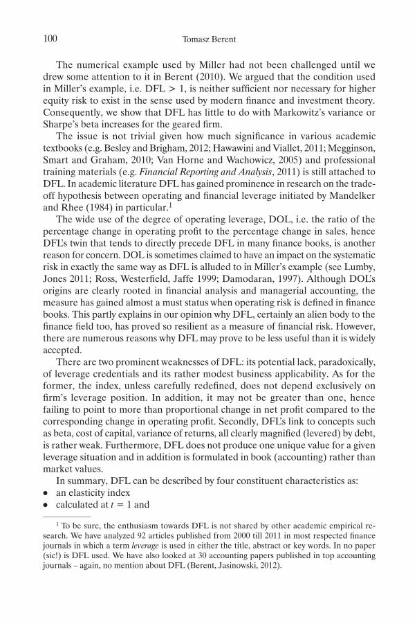
Figure 1DFL as a function of debt ratio D/(E + D), ROIC > i

0

1

2

3

0% 20% 40% 60% 80% 100%D/(D + E)

DFL

source: own calculation.

Some authors ignore the question altogether by simply assuming that financial leverage is what DFL measures; after all, more debt means higher DFL – they seem to claim. True, DFL grows with higher debt ratio D/(E + D) inter alia just like one would expect financial leverage to behave (see Figure 1). Yet it is not always true. DFL is a rational function of D/(E + D), defined for 0 G D/(E + D) G 1, where ROIC ! 0, ROIC ! i×D/(E + D) and the cost of debt i > 0% but it is a continuous increasing function within its domain only if ROIC > i.2

No doubt a clear definition of financial leverage would help.3 However, given the state of chaos in the leverage literature, to which miller seems to contribute, we may be better advised to proceed with merely a tentative agreement that financial leverage is the phenomenon associated with the increased risk/volatility, regardless of how measured, introduced by firm’s financial activity. Surprisingly, even with such a vague working definition, if only rigorous analysis is strictly followed, a number of meaningful findings can be established.

Should DFL depend on taxes?Net profit in (1) is influenced by both interest payment and taxes. While interest payment is clearly a constituent part of firm’s financial activity, the leverage

2 The function has a vertical asymptote at D/(E + D) = ROIC/i that falls within the domain of the acceptable debt ratio values if 0 G ROIC G i; the function may even be decreasing if ROIC < 0.

3 The proper definition of financial leverage deserves a separate treatment. In Berent 2011a, a very general definition of financial leverage risk is proposed that focuses on the increased probability of gene-rating extreme (negative and/or positive) values of returns. The definition is useful in that it enables the definition user to decide the way how “extreme values” should be understood. This allows more specific definitions to be proposed. We argue that most of definitions present in the literature can be derived from this general approach.


credentials of taxes are less obvious. The different tax regimes may lead to different values of DFL. The question arises whether this impact is a legitimate part of leverage analysis or not?

Are operating results independent of capital structure?DFL definition in (1) does not seem to address a vital question about the interrelation between operating and financial decisions. The EBIT level in (1) may or may not be influenced by the amount of debt taken. However, just like in the case of taxes, a legitimate question arises if any financial leverage index should capture the total effect of debt taking or maybe merely this portion that excludes financial activity impact on operations.

What are the base and end profit values in DFL?The DFL definition does not elaborate much on the nature of profit numbers in (1). What are the criteria for their choice? Are they to be e.g. last year’s numbers, next year’s management forecasts or market expectations? Can any arbitrarily chosen profit level serve as the base? What about end values? Should they be viewed as different potential scenarios or simply differences from the expected (base) level? Consequently, what is the meaning of the profit change in (1)? Is it simply the deviation from the benchmark when the base and end profits belong to the same time period, or is it rather the ‘percentage change’ across time – the case when the base and end profit numbers belong to different time periods. If profit numbers are taken from two different time periods, what period: base or end, is actually described by DFL? What happens if, for example, different capital structures or/and different interest payments, prevail in those two periods?

Does the size of EBIT change matter?Another issue concerns the significance of ‘a 1% EBIT change’ interpretation. Does this interpretation imply that DFL is only about a 1% EBIT change or that the change in EBIT can be arbitrarily large? If so, is DFL identical for all sizes of EBIT change? Is it possible that a 1% change in EBIT generates, say, a 3% change in EAT, but a 10% change in EBIT generates, say, a 20% change in EAT? If ‘yes’, which DFL value, 3.0 or 2.0, is valid? This leads to a question whether financial risk (however measured) should depend on the size of EBIT change at all.

What is DFL calculated for?even a detailed literature review does not give an unambiguous answer to the question about DFL’s application. Generally, there are two ways DFL is used: either as a financial risk measure or as a financial analysis tool. In the first and most popular approach, DFL – usually calculated for a set of hypothetical profit numbers – is claimed to quantify the financial risk of equity when debt is taken. The reason for this interpretation is that DFL tends to be greater than one for a geared company. The rule that follows seems simple: the higher DFL, the higher both earnings volatility and financial risk. The problem however is that the numerical examples in the books are deliberately set so that DFL > 1.

Tomasz Berent104

Unfortunately, most authors writing about DFL fail to mention that DFL does not have to be greater than one.

Another point regarding the application of DFL as a risk measure is the question whether it is acceptable that any financial risk indicator should generate more than one unique value for one unique state of financial activity. It looks rather odd when a given capital structure produces many different financial leverage values. The immediate question is which of many values is relevant in capturing financial risk.

DFL as an analytical tool is used to explain or forecast net profit reaction caused by a given operating profit change. Although a leverage interpretation is not needed in this approach, it tends to be present here as well since numerical examples used in textbooks are construed so that DFL is again greater than one.

In the following sections, we attempt to address all the issues raised above in more detail. First, some initial assumptions are proposed to clear off the immediate concerns related to the definition (1).

2. DFL – static version and investor’s perspective

A closer inspection of (1) reveals that DFL can be decomposed into three factors:

.

.

.

%%

( )( )

( )( )

( )( )

%%

%%

(1 )( )

%%

( )( )

%%

,

( ) ( %)

( ) [ %]

*

( )( )

( )

( )

( )

( )

( )

( )

%%

( )( )

( )( )

DFLEBITEAT

EBIT EBITEAT EAT

EATEBIT

DFLEBIT INT

EBITETRMTR

EBIT EBITINT INT

DFLEBIT INT

EBIT

DFLEATEAT

EATEAT

EATEAT

DFLEV

DFLEV

EBIT INTEV EBIT

DFLEV

ROEEV ROE

DFLE EV

DFL DFL DFL

DFLEV EV

DFLEV

DFL DFL DFL

DFLX

X

EDFL

SEN

ELA

ELASEN

EE

EE

EE

EE D

EE

E

E E

E E

EE

E EE

E EE D

w w

E E kk

EE

EE

EE

E EE D

w w

Ek

E kE

Ek

E kE

E D

E

EE D

k w k w k

rr

N

r k

N

r k

NE

ENE

E E

NE

E ENE

E E

XY

XY

M

MEE

E kE k

kk

11

1

1

11

11 1

1

1 1

11

11

stdevstdev

i

B

B

B

B

B B

B

B B

B

B

B

U

G

U

G

GB

UB

WU

G

U

G

GB

UB

GB

UB

GB

B

WGB

B

B

B

WGB

B

UB

GB

WU

G

U

G

GB

UB

W W

WGB

B

G

U

WU

G

U

G

GB

UB

W W

W

U

U

U UU

G

G

G GG

G G U

U

G

Ui U

N

Gi Gi

N

UB

Ui UB

i

N

GB

Gi GB

i

N

UB

Ui UB

i

N

GB

Gi GB

i

N

W

UB

GB

UB U

GB G

U

G

0

0 0

0

0

0

0

00

0

0

0

0

0

0

0

0

0 0

1 0 2

0

0

00

0

0

0

0

0

0

0

0

0 0

1 0 2

0

00

0

00

1 2

2

2

02

2

02

2

2

2

2

2

0

0

# #

#

# #

#

#

#

# #

#

#

# #

# #

# # #

#

#

#

#

# #

!

D

D

D

D

D

D

D

D

D

D D

D

D

D

D

D

D

D

D

D

D

D

=- -

--

-

-

=-

= =

= = =+

=

= =+ -

+

= =+

+

= = = =+

= +

= =+

+

= +

=

+

+ +-

+

+ ++

-

=+

=

-

-

=-

-

-

-

=

=

=

= =+

+=

+

+

= =-

-

= = = =+

= +

=

= G

!

!

!

!

!

!

, (2)

where eTrB = TAXB/eBTB is a base period effective tax rate, i.e. the share of tax payment TAXB in earnings before taxes eBTB, while mTr = (TAX – TAXB)/(eBT – eBTB) denotes a tax rate at which the difference between the end and base levels of pre-tax profits, i.e. (EBT – EBTB), is taxed knowing that the initial portion of eBT, equal to eBTB, is taxed at eTrB.

The first component of (2) describes the base value of operating and pre-tax profit, the second describes taxes, while the third is determined by the size of the profit change. If the tax component is split into two: 1/(1 – ETRB) and (1 – mTr), and subsequently allocated to the base values and to the change in profits components respectively, then DFL can be viewed as consisting of only two components: one describing the base, the other - the profit changes from this base.

According to (2), DFL assumes different values inter alia for different levels of: operating profit base EBITB, change in operating profit DEBIT = EBIT – EBITB, base interest payment INTB, change in interest payment DINT = INT – INTB, and taxes. DFL does therefore depend on factors, e.g. taxes, which may not be regarded as legitimate constituents of financial leverage; secondly, the size of DFL depends on the difference between interest paid in the base period and the end period; thirdly, DFL assumes different values for different sizes of EBIT change.


Even without problems brought about by DFL’s dependence on EBITB and INTB – discussed in section 3 in more detail – these three points alone make DFL dubious as a leverage measure.

Table 1 illustrates the scale of the problem with the help of a numerical example, when a 1% (columns A1, B1, C1) and a 10% EBIT change (columns A10, B10, C10) from the base value of EBITB = 40 are assumed. In the end period, three different scenarios with different levels of ETR and INT are studied. As a result, DFL ranges from 1.33 to 3.0 depending on the size of EBIT change (B1 ! B10, C1 ! C10), the interest payment (A1 ! C1, A10 ! C10) and taxes paid (A1 ! B1, A10 ! B10).

Table 1DFL for different INT and TAX

Base A1 B1 C1 A10 B10 C10

EBIT 40.00 40.40 40.40 40.40 44.00 44.00 44.00

INT –10.00 –10.00 –10.00 –9.50 –10.00 –10.00 –9.50

eBT 30.00 30.40 30.40 30.90 34.00 34.00 34.50

eTr 20.0% 20.00% 19.80% 20.00% 20.00% 19.80% 20.00%

TAX –6.00 –6.08 –6.02 –6.18 –6.80 –6.73 –6.90

eAT 24.00 24.32 24.38 24.72 27.20 27.27 27.60

mTr 20.00% 4.80% 20.00% 20.00% 18.30% 20.00%

D%EBIT 1.00% 1.00% 1.00% 10.00% 10.00% 10.00%

D%eAT 1.33% 1.59% 3.00% 13.33% 13.62% 15.00%

DFL 1.33 1.59 3.00 1.33 1.36 1.50


2.1. Additional assumptions

Below two additional assumptions to model (1) are added, clarifying how DFL should be understood.

Assumption 1: one period analysisAssumption 1 calls for the interpretation of the change in profit in (1) to be the deviation of the end profit from its base level that is generated at the same time period. Across-time growth rates are excluded.4 Assumption 1 bans DFL calculations with historic profit levels used as the base and future profit forecasts used as analyzed scenarios. Limiting analysis to one period solves many problems. First and foremost, interest payment is made fixed so that INT = INTB (from now on referred to as INT). This makes the third component of (2) to disappear and

4 This does not ‘prohibit’ the calculation of the ratio of relative changes in EBIT and EAT across time. We only claim that such a ratio should no longer be regarded as a leverage index in general and DFL in particular.

Tomasz Berent106

leads to the conclusion that the change in EBIT is not important.5 Furthermore, as DFL is now blind to the size of DEBIT, discrete mathematics can successfully be replaced by differential calculus. moreover, mTr in (2) becomes a standard marginal tax rate as defined by the tax law rather than an artificially defined tax rate at which the marginal across-time change in eBT is taxed. note, with DINT = 0, a unit change in EBIT results in (1 – MTR) unit change in EAT, which together with eATB = eBTB×(1 – eTrB) leads directly from (1) to (2).

Assumption 2: no taxesWe believe that tax impact on earnings volatility is not a part of financial leverage and should be analyzed separately. Although in assumption 2 we explicitly assume no taxes, one should note that for DFL to be tax-indifferent, it would be sufficient to assume that mTr is equal to eTrB. Although it was first noticed by Dilbeck (1962) many years ago, this assumption is hardly mentioned in the DFL literature. In a multi bracket tax regime, ETRB may always happen by coincidence to equal MTR, but this could be true for a given size of EBIT change only. If a linear corporate tax code – true for most legislations – and no differences between tax and financial accounting are assumed, then ETRB is indeed equal to mTr.6

2.2. Static version of DFL

After two assumptions are made, formula (2) folds down to what is usually known in literature as a “static” version of DFL as opposed to ‘dynamic’ in (1):

.

.

.

%%

( )( )

( )( )

( )( )

%%

%%

(1 )( )

%%

( )( )

%%

,

( ) ( %)

( ) [ %]

*

( )( )

( )

( )

( )

( )

( )

( )

%%

( )( )

( )( )

DFLEBITEAT

EBIT EBITEAT EAT

EATEBIT

DFLEBIT INT

EBITETRMTR

EBIT EBITINT INT

DFLEBIT INT

EBIT

DFLEATEAT

EATEAT

EATEAT

DFLEV

DFLEV

EBIT INTEV EBIT

DFLEV

ROEEV ROE

DFLE EV

DFL DFL DFL

DFLEV EV

DFLEV

DFL DFL DFL

DFLX

X

EDFL

SEN

ELA

ELASEN

EE

EE

EE

EE D

EE

E

E E

E E

EE

E EE

E EE D

w w

E E kk

EE

EE

EE

E EE D

w w

Ek

E kE

Ek

E kE

E D

E

EE D

k w k w k

rr

N

r k

N

r k

NE

ENE

E E

NE

E ENE

E E

XY

XY

M

MEE

E kE k

kk

11

1

1

11

11 1

1

1 1

11

11

stdevstdev

i

B

B

B

B

B B

B

B B

B

B

B

U

G

U

G

GB

UB

WU

G

U

G

GB

UB

GB

UB

GB

B

WGB

B

B

B

WGB

B

UB

GB

WU

G

U

G

GB

UB

W W

WGB

B

G

U

WU

G

U

G

GB

UB

W W

W

U

U

U UU

G

G

G GG

G G U

U

G

Ui U

N

Gi Gi

N

UB

Ui UB

i

N

GB

Gi GB

i

N

UB

Ui UB

i

N

GB

Gi GB

i

N

W

UB

GB

UB U

GB G

U

G

0

0 0

0

0

0

0

00

0

0

0

0

0

0

0

0

0 0

1 0 2

0

0

00

0

0

0

0

0

0

0

0

0 0

1 0 2

0

00

0

00

1 2

2

2

02

2

02

2

2

2

2

2

0

0

# #

#

# #

#

#

#

# #

#

#

# #

# #

# # #

#

#

#

#

# #

!

D

D

D

D

D

D

D

D

D

D D

D

D

D

D

D

D

D

D

D

D

D

=- -

--

-

-

=-

= =

= = =+

=

= =+ -

+

= =+

+

= = = =+

= +

= =+

+

= +

=

+

+ +-

+

+ ++

-

=+

=

-

-

=-

-

-

-

=

=

=

= =+

+=

+

+

= =-

-

= = = =+

= +

=

= G

!

!

!

!

!

!

(3)

The static version of DFL is fully determined by firm’s income statement and hence easy to calculate. This simplicity is not achieved at no cost: by stripping (1) of end values, the static version of DFL is void of its explicit elasticity (dynamic) interpretation. The dynamic and static forms of DFL are equivalents only if the two assumptions mentioned above are made.

2.3. Investor’s perspective

With no taxes, EBIT in (1) can be interpreted as the net profit of an all equity firm, EATU. Then DFL becomes a ratio of the relative change in net profit EATG

5 Some caution is advised here. The size of the EBIT change may affect DFL indirectly via the second component unless tax rates do not depend on the size of EBIT. If this is not true, the irrelevance of the EBIT size change is secured only after further assumptions on taxes are made (see Assumption 2).

6 If one restricts DFL to the first component of (2) when MTR ! eTrB, then DFL is interpreted as a ratio of relative changes in EAT and EBIT that implicitly assumes MTR = ETRB with the difference between DFL and the ratio of actual changes being attributed to taxes.


of the geared company to the relative change in net profit EATU of the otherwise identical firm with no debt:

.

.

.

%%

( )( )

( )( )

( )( )

%%

%%

(1 )( )

%%

( )( )

%%

,

( ) ( %)

( ) [ %]

*

( )( )

( )

( )

( )

( )

( )

( )

%%

( )( )

( )( )

DFLEBITEAT

EBIT EBITEAT EAT

EATEBIT

DFLEBIT INT

EBITETRMTR

EBIT EBITINT INT

DFLEBIT INT

EBIT

DFLEATEAT

EATEAT

EATEAT

DFLEV

DFLEV

EBIT INTEV EBIT

DFLEV

ROEEV ROE

DFLE EV

DFL DFL DFL

DFLEV EV

DFLEV

DFL DFL DFL

DFLX

X

EDFL

SEN

ELA

ELASEN

EE

EE

EE

EE D

EE

E

E E

E E

EE

E EE

E EE D

w w

E E kk

EE

EE

EE

E EE D

w w

Ek

E kE

Ek

E kE

E D

E

EE D

k w k w k

rr

N

r k

N

r k

NE

ENE

E E

NE

E ENE

E E

XY

XY

M

MEE

E kE k

kk

11

1

1

11

11 1

1

1 1

11

11

stdevstdev

i

B

B

B

B

B B

B

B B

B

B

B

U

G

U

G

GB

UB

WU

G

U

G

GB

UB

GB

UB

GB

B

WGB

B

B

B

WGB

B

UB

GB

WU

G

U

G

GB

UB

W W

WGB

B

G

U

WU

G

U

G

GB

UB

W W

W

U

U

U UU

G

G

G GG

G G U

U

G

Ui U

N

Gi Gi

N

UB

Ui UB

i

N

GB

Gi GB

i

N

UB

Ui UB

i

N

GB

Gi GB

i

N

W

UB

GB

UB U

GB G

U

G

0

0 0

0

0

0

0

00

0

0

0

0

0

0

0

0

0 0

1 0 2

0

0

00

0

0

0

0

0

0

0

0

0 0

1 0 2

0

00

0

00

1 2

2

2

02

2

02

2

2

2

2

2

0

0

# #

#

# #

#

#

#

# #

#

#

# #

# #

# # #

#

#

#

#

# #

!

D

D

D

D

D

D

D

D

D

D D

D

D

D

D

D

D

D

D

D

D

D

=- -

--

-

-

=-

= =

= = =+

=

= =+ -

+

= =+

+

= = = =+

= +

= =+

+

= +

=

+

+ +-

+

+ ++

-

=+

=

-

-

=-

-

-

-

=

=

=

= =+

+=

+

+

= =-

-

= = = =+

= +

=

= G

!

!

!

!

!

!

. (4)

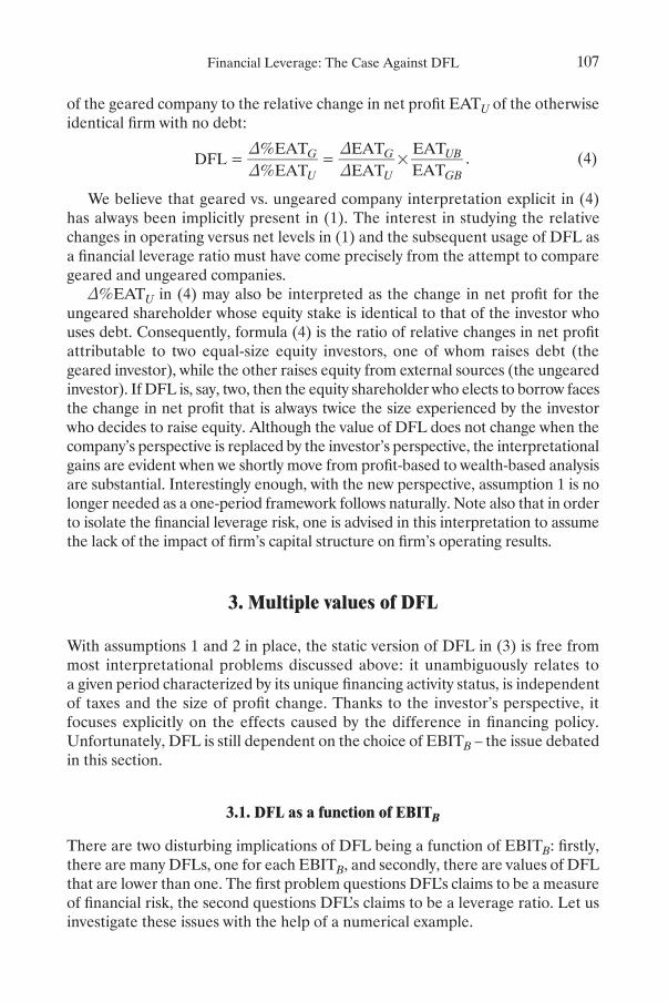
We believe that geared vs. ungeared company interpretation explicit in (4) has always been implicitly present in (1). The interest in studying the relative changes in operating versus net levels in (1) and the subsequent usage of DFL as a financial leverage ratio must have come precisely from the attempt to compare geared and ungeared companies.D%eATU in (4) may also be interpreted as the change in net profit for the

ungeared shareholder whose equity stake is identical to that of the investor who uses debt. Consequently, formula (4) is the ratio of relative changes in net profit attributable to two equal-size equity investors, one of whom raises debt (the geared investor), while the other raises equity from external sources (the ungeared investor). If DFL is, say, two, then the equity shareholder who elects to borrow faces the change in net profit that is always twice the size experienced by the investor who decides to raise equity. Although the value of DFL does not change when the company’s perspective is replaced by the investor’s perspective, the interpretational gains are evident when we shortly move from profit-based to wealth-based analysis are substantial. Interestingly enough, with the new perspective, assumption 1 is no longer needed as a one-period framework follows naturally. note also that in order to isolate the financial leverage risk, one is advised in this interpretation to assume the lack of the impact of firm’s capital structure on firm’s operating results.

3. Multiple values of DFL

With assumptions 1 and 2 in place, the static version of DFL in (3) is free from most interpretational problems discussed above: it unambiguously relates to a given period characterized by its unique financing activity status, is independent of taxes and the size of profit change. Thanks to the investor’s perspective, it focuses explicitly on the effects caused by the difference in financing policy. Unfortunately, DFL is still dependent on the choice of EBITB – the issue debated in this section.

3.1. DFL as a function of EBITB

There are two disturbing implications of DFL being a function of EBITB: firstly, there are many DFLs, one for each EBITB, and secondly, there are values of DFL that are lower than one. The first problem questions DFL’s claims to be a measure of financial risk, the second questions DFL’s claims to be a leverage ratio. Let us investigate these issues with the help of a numerical example.

Tomasz Berent108

ExampleLet company’s invested capital be IC = 100 and initial equity capital E0 = 50. The shareholder is to decide how to fill the financing gap. Should he raise debt D0 = 50, he remains the only shareholder in a levered firm with debt-to-equity ratio of D0/E0 = 1. should he raise external equity of 50 by inviting a co-owner, he holds a 50% equity stake in the all-equity company. The cost of debt is i = 10%, hence interest payment amounts to INT = i × D0 = 5. no taxes are assumed.

Table 2DFL and a –10% change in net profit for the ungeared investor

EB

ITB

eA

TU

B

eA

TG

B

EB

IT

eA

TU

eA

TG

D%

eA

TU

D%

eA

TG

DFL

Lev

erag

e

A 50.0 25.0 45.0 45.0 22.5 40.0 –10.0% –11.1% 1.11 yes

B 20.0 10.0 15.0 18.0 9.0 13.0 –10.0% –13.3% 1.33 yes

C 6.0 3.0 1.0 5.4 2.7 0.4 –10.0% –60.0% 6.00 yes

D 4.0 2.0 –1.0 3.6 1.8 –1.4 –10.0% 40.0% –4.00 ?

e 2.0 1.0 –3.0 1.8 0.9 –3.2 –10.0% 6.7% –0.67 no

F –4.0 –2.0 –9.0 –3.6 –1.8 –8.6 –10.0% –4.4% 0.44 no


Table 3DFL and a +10% change in net profit for the ungeared investor

EB

ITB

eA

TU

B

eA

TG

B

EB

IT

eA

TU

eA

TG

D%

eA

TU

D%

eA

TG

DFL

Lev

erag

e

A 50.0 25.0 45.0 55.0 27.5 50.0 10.0% 11.1% 1.11 yes

b 20.0 10.0 15.0 22.0 11.0 17.0 10.0% 13.3% 1.33 yes

c 6.0 3.0 1.0 6.6 3.3 1.6 10.0% 60.0% 6.00 yes

d 4.0 2.0 –1.0 4.4 2.2 –0.6 10.0% –40.0% –4.00 ?

e 2.0 1.0 –3.0 2.2 1.1 –2.8 10.0% –6.7% –0.67 no

f –4.0 –2.0 –9.0 –4.4 –2.2 –9.4 10.0% 4.4% 0.44 no


Tables 2 and 3 summarize net profit changes for the geared shareholder when the net profit for the ungeared one changes by –10% and +10%:

For EBIT 1 B = 50, DFL = 1.11, hence a 10% increase (decrease) in net profit from 25.0 to 27.5 (22.5) when ungeared corresponds to an 11.1% increase (decrease)


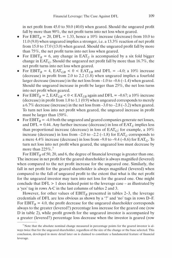
in net profit from 45.0 to 50.0 (40.0) when geared. Should the ungeared profit fall by more than 90%, the net profit turns into net loss when geared.For EBIT 1 B = 20, DFL = 1.33, hence a 10% increase (decrease) from 10.0 to 11.0 (9.0) when ungeared implies a stronger, i.e. a 13.3% reaction of net profit from 15.0 to 17.0 (13.0) when geared. Should the ungeared profit fall by more than 75%, the net profit turns into net loss when geared.For EBIT 1 B = 6, any change in EATU is accompanied by a six fold bigger change in eATG. Should the ungeared net profit fall by more than 16.7%, the net profit turns into net loss when geared.For EBIT 1 B = 4, eATGB < 0 < EATUB and DFL = –4.0; a 10% increase (decrease) in profit from 2.0 to 2.2 (1.8) when ungeared implies a fourfold larger decrease (increase) in the net loss from –1.0 to –0.6 (–1.4) when geared. Should the ungeared increase in profit be larger than 25%, the net loss turns into net profit when geared. For EBIT 1 B = 2, eATGB < 0 < EATUB again and DFL = –0.67; a 10% increase (decrease) in profit from 1.0 to 1.1 (0.9) when ungeared corresponds to merely a 6.7% decrease (increase) in the net loss from –3.0 to –2.8 (–3.2) when geared. To turn net loss into net profit when geared, the ungeared increase in profit must be larger than 150%.For EBIT 1 B = -4.0 both the ungeared and geared companies generate net losses, and DFL = 0.44. Any further increase (decrease) in loss of eATU implies less than proportional increase (decrease) in loss of eATG; for example, a 10% increase (decrease) in loss from –2.0 to –2.2 (–1.8) for eATU corresponds to a mere 4.4% increase (decrease) in loss from –9.0 to –9.4 (–8.6) for EATG. To turn net loss into net profit when geared, the ungeared loss must decrease by more than 225%.7For EBITB of 50, 20, and 6, the degree of financial leverage is greater than one.

The increase in net profit for the geared shareholder is always magnified (levered) when compared to the net profit increase for the ungeared one. Similarly, the fall in net profit for the geared shareholder is always magnified (levered) when compared to the fall of ungeared profit to the extent that what is the net profit for the ungeared investor may turn into net loss for the geared one. one might conclude that DFL > 1 does indeed point to the leverage case – as illustrated by a ‘yes’ tag in rows A-C in the last columns of tables 2 and 3.

However, for other values of EBITB presented in tables 2–3, the leverage credentials of DFL are less obvious as shown by a ‘?’ and ‘no’ tags in rows D–F. For EBITB = 4.0, the profit decrease for the ungeared shareholder corresponds always to the greater (levered?) percentage loss increase for the geared one (row D in table 2), while profit growth for the ungeared investor is accompanied by a greater (levered?) percentage loss decrease when the investor is geared (row

7 note that the absolute nominal change measured in percentage points for the geared investor is al-ways twice that for the ungeared shareholder, regardless of the size of the change or the base selected. This conclusion, developed in more detail later on is claimed to constitute a fundamental feature of financial leverage.

Tomasz Berent110

D in table 3). Does the case, where the ungeared shareholder shows profit, while the geared one shows losses, but the percentage changes in losses for the latter are bigger than the percentage changes in net profit for the former, describe leverage? We do not think so. Far less controversy is spurred by the last two rows E-F of the tables 2–3, where, for EBITB = 2 and EBITB = –4, DFL is lower than one. Any change in the net profit/loss when ungeared is accompanied by less than proportional change in the net loss when geared. Formula (4) continues to correctly, mathematically speaking, describe the profit dynamics for the geared versus ungeared shareholders, however, to claim that DFL retains leverage characteristics is no longer justified.

Table 4DFL as a function of EBITB

EBITB vs. INT > 0 DFL

EBITB > INT DFL > 1

EBITB = INT DFL does not exist

INT/2 < EBITB < INT DFL < –1

EBITB = INT/2 DFL = –1

0 < EBITB < INT/2 –1 < DFL < 0

EBITB = 0 DFL does not exist

EBITB < 0 0 < DFL < 1


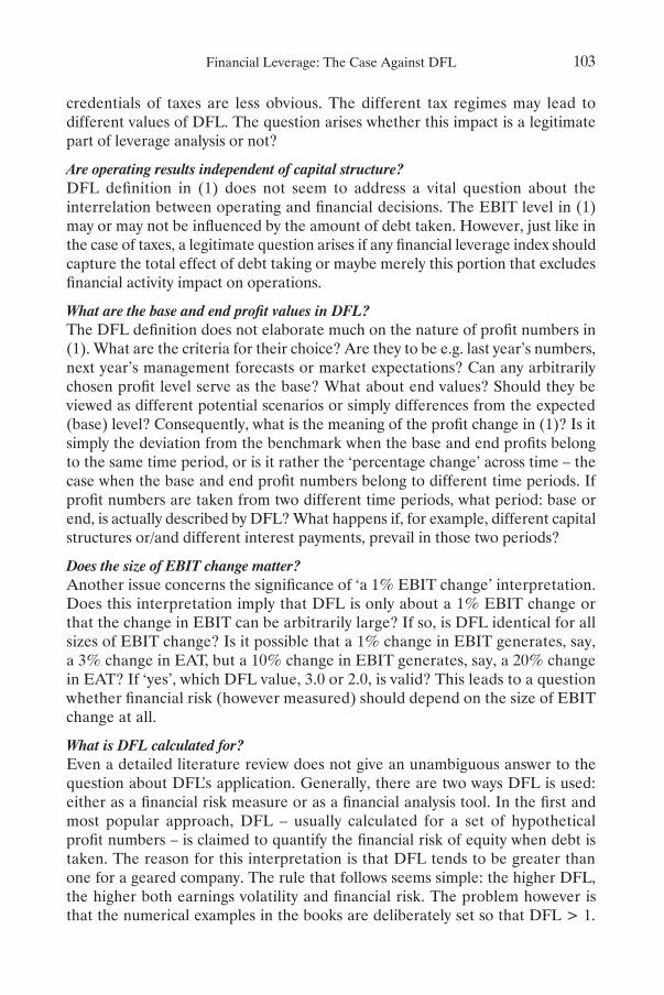
Figure 2DFL as a function of EBITB ! INT and EBITB ! 0

–5

–4

–3

–2

–10

1

2

3

4

5

–10 –5 5 10 15 20

DFL

EBITB



Figure 2 illustrates DFL as a function of EBITB for 0 ! EBITB ! INT using parameter values from our numerical example. Table 4 lists all the values of DFL in an algebraic form. DFL is greater than one only when EBITB > INT, where net profits for both the ungeared and geared investors are positive.8

3.2. Is the multiple value nature of DFL a real problem?

If DFL, when lower than one, cannot be interpreted as a leverage ratio, it cannot be a financial risk measure either. Its claims to be a financial risk measure vastly improve if the analysis is limited to the cases where DFL > 1. Indeed, it is usually this case that is discussed in the DFL literature (unfortunately, in most cases with no mention that other cases are also possible). Then, it is argued that the higher EBITB, the lower financial risk (via lower DFL); the lower EBITB, the higher financial risk (via higher DFL). High EBITB in relation to INT allegedly implies lower chances of making losses, while a low (close to INT) value of EBITB allegedly implies higher chances of going into the red. However, this reasoning is only correct in the context of the expected value of EBIT: the drop in the expected value of EBIT does indeed elevate inter alia the risk of registering lower and negative values of net profit or even going bankrupt for the geared investor. This is however not applicable to DFL calculation based on an often arbitrary chosen EBITB.

There is little one can do to prevent analysts from calculating DFL for any level of EBITB > INT they wish, but then such an index says nothing about the financial risk involved. If this arbitrarily chosen value of EBITB is much higher than the company’s interest payment INT, it does not mean that the risk of the venture is low but merely it means that the benchmark used in calculation is high. Ultimately, DFL is the information about the choice of the base value of EBITB rather than about the risk, let alone systematic risk.9

3.3. DFL as a language convention

If DFL, with its propensity to produce many values, is not a measure of financial risk, then what it is? Berent (2011b) proposes to treat different DFL’s as different languages to communicate the information on a given EBIT change. From this perspective, the user of DFL has the right to choose any arbitrary level of EBITB as long as 0 ! EBITB ! INT. Each EBITB leads to a different language and different narrative. The problems with multiple DFLs or DFL < 1 vanish as a result. If DFL > 1, the language used possesses a leverage interpretation, if DFL < 1, the leverage interpretation is simply not available.

8 Note that DFL cannot be calculated for EBITB = INT and EBITB = 0. Yet financial risk has not ceased to exist only because DFL cannot be calculated.

9 Berent (2011b) reviews many other potential arguments used in the defense of a multiple value nature of DFL and explains why they are all flawed.

Tomasz Berent112

DFL is no longer perceived as a single value risk measure but as a multiple value communication or financial analysis tool. For example, if the scenario that produces EBIT = 18 is contemplated then it can be communicated in many different ways (see table 5). With the base of 20 or 50, this scenario means a decline for the ungeared investor, while with the base of 6, 4, 2 or –4 it denotes an improvement relative to the base. more interestingly, this scenario for the geared investor is communicated by DFLs that range from –4.0 to +6.0. With the base of 50, the scenario implies a drop of 64% for the ungeared investor but more than a 71% drop for the geared one (DFL = 1.11). With the base of 20, the scenario implies a drop of 10% when ungeared and more than 13% when geared (DFL = 1.33). With the base of 6, the scenario means 200% growth when ungeared and a magnificent 1200% growth when geared (DFL = 6). The presence of financial leverage forces is apparent here.

However, with the base of 2.0, the scenario implies 800% growth in net profit when ungeared and a mere 533% drop in net loss when geared (DFL = -0.67), while with the base of –4, the scenario implies 550% drop in net profit when ungeared but only a 244% drop when geared (DFL = 0.44). The narrative changes significantly and leverage is no longer so obvious.

Table 5EBIT = 18 communicated in different languages via different DFLs

EB

ITB

eA

TU

B

eA

TG

B

EB

IT

eA

TU

eA

TG

D%

eA

TU

D%

eA

TG

DFL

A 50.0 25.0 45.0 18.0 9.0 13.0 –64.0% –71.1% 1.11

B 20.0 10.0 15.0 18.0 9.0 13.0 –10.0% –13.3% 1.33

C 6.0 3.0 1.0 18.0 9.0 13.0 200.0% 1200.0% 6.00

D 4.0 2.0 –1.0 18.0 9.0 13.0 350.0% –1400.0% –4.00

e 2.0 1.0 –3.0 18.0 9.0 13.0 800.0% –533.3% –0.67

F –4.0 –2.0 –9.0 18.0 9.0 13.0 –550.0% –244.4% 0.44


The existence of many mathematically legitimate bases does not mean that all bases are equally useful. For the base to be acceptable, it must have some business or economic justification. Hence the acceptable bases are those, which describe, for instance, management forecasts, market expectations, most optimistic or most pessimistic scenarios, or (with due care regarding the comparability of the periods) last year’s or other historic results etc. against which deviations are measured. If the base leads to DFL > 1 the language used is easy to understand and offers a leverage story, if DFL < 1 it is far less intuitive as a communication tool.


3.4. Is one unique DFL value possible?

There is still one more alternative explanation of a multiple DFL dilemma available. What if there exists a single, unique level of EBITB that leads to one unique level of DFL with all other values being simply irrelevant. The calculation of many DFLs would then be a mistake made by DFL users rather than the flaw of the index itself. How should such a base be searched for if it does exist? one thing is clear: as accounting is itself a set of various conventions, the proper base is certainly not to be found within the accounting world of a standard version of DFL. The issue is taken up in the next section when market values are introduced.

4. DFL reformulation

To restore DFL as a true leverage and financial risk index, significant modifications to its definition are required. Below we tackle each of the DFL constituent features separately.

4.1. Profit vs. wealth perspective

DFL is formulated in terms of profit numbers, i.e. in terms of (book value) annual wealth changes rather than wealth levels themselves. The attractiveness of this approach is not surprising given the importance of financial reporting. Indeed, publishing periodic results has become one of the most important ways of communicating to the public firm’s financial health.10 However, as a profit constitutes merely a fraction of investor’s wealth, focusing on profit is precarious. some may argue that the analysis of wealth changes can always be translated into the analysis of wealth as: W1 = W0 + DW, where DW is the change in wealth between t = 0 and t = 1. The problem arises when the metrics based on wealth changes are only loosely linked to those based on wealth itself: what is clear for a wealth level may no longer be so for a wealth change. This unfortunately may be the case with DFL.

In particular, the fact that DFL gets lower than one, a disqualifying feature for a profit based DFL, ceases to be a problem for a wealth based DFL. The argument is now developed in more detail. Let’s reformulate DFL in terms of (book value) wealth rather than in terms of an accounting profit, with EU and EG being book value wealth levels for the ungeared and geared equity holder respectively. The wealth levels encompass accumulated earnings so that

10 It may be argued that financial results releases are partly responsible for a gradual replacement of finance perspective by accounting perspective in analyzing firm’s financial performance. ‘Profit’ has proved to be an easier concept than ‘value’. DFL methodology is clearly an accounting and hence an alien implant into the way finance theory should study financial leverage.

Tomasz Berent114

EG = EGB0 + eATG and eU = EUB0 + eATU, where subscript 0 denotes wealth before net profit. The wealth the ungeared and geared investors start with at t = 0 is by definition identical EUB0 = EGB0 = E0. Wealth of the ungeared investor EU can always (at t = 0 as well as t = 1) be thought of as a constant fraction E0/(D0 + E0) of the total enterprise value EV, and EV is assumed not to depend on firm’s capital structure. Then a wealth based DFLW, with a subscript W to distinguish it from the profit based DFL, is a ratio of a percentage change in (cum profit) wealth for the geared investor that corresponds to a 1% change in (cum profit) wealth for the ungeared investor:

.

.

.

%%

( )( )

( )( )

( )( )

%%

%%

(1 )( )

%%

( )( )

%%

,

( ) ( %)

( ) [ %]

*

( )( )

( )

( )

( )

( )

( )

( )

%%

( )( )

( )( )

DFLEBITEAT

EBIT EBITEAT EAT

EATEBIT

DFLEBIT INT

EBITETRMTR

EBIT EBITINT INT

DFLEBIT INT

EBIT

DFLEATEAT

EATEAT

EATEAT

DFLEV

DFLEV

EBIT INTEV EBIT

DFLEV

ROEEV ROE

DFLE EV

DFL DFL DFL

DFLEV EV

DFLEV

DFL DFL DFL

DFLX

X

EDFL

SEN

ELA

ELASEN

EE

EE

EE

EE D

EE

E

E E

E E

EE

E EE

E EE D

w w

E E kk

EE

EE

EE

E EE D

w w

Ek

E kE

Ek

E kE

E D

E

EE D

k w k w k

rr

N

r k

N

r k

NE

ENE

E E

NE

E ENE

E E

XY

XY

M

MEE

E kE k

kk

11

1

1

11

11 1

1

1 1

11

11

stdevstdev

i

B

B

B

B

B B

B

B B

B

B

B

U

G

U

G

GB

UB

WU

G

U

G

GB

UB

GB

UB

GB

B

WGB

B

B

B

WGB

B

UB

GB

WU

G

U

G

GB

UB

W W

WGB

B

G

U

WU

G

U

G

GB

UB

W W

W

U

U

U UU

G

G

G GG

G G U

U

G

Ui U

N

Gi Gi

N

UB

Ui UB

i

N

GB

Gi GB

i

N

UB

Ui UB

i

N

GB

Gi GB

i

N

W

UB

GB

UB U

GB G

U

G

0

0 0

0

0

0

0

00

0

0

0

0

0

0

0

0

0 0

1 0 2

0

0

00

0

0

0

0

0

0

0

0

0 0

1 0 2

0

00

0

00

1 2

2

2

02

2

02

2

2

2

2

2

0

0

# #

#

# #

#

#

#

# #

#

#

# #

# #

# # #

#

#

#

#

# #

!

D

D

D

D

D

D

D

D

D

D D

D

D

D

D

D

D

D

D

D

D

D

=- -

--

-

-

=-

= =

= = =+

=

= =+ -

+

= =+

+

= = = =+

= +

= =+

+

= +

=

+

+ +-

+

+ ++

-

=+

=

-

-

=-

-

-

-

=

=

=

= =+

+=

+

+

= =-

-

= = = =+

= +

=

= G

!

!

!

!

!

!

, (5)

where EUB, EGB, and eVB denote the base values of wealth at t = 1 for the ungeared and geared investors as well as for the whole enterprise respectively. As illustrated by (5), DFLW proves to be an equity multiplier at t = 1 determined by the base levels of capital at t = 1.

Equation (6) offers the formulation of DFLW as a function of the base value of EBITB:

.

.

.

%%

( )( )

( )( )

( )( )

%%

%%

(1 )( )

%%

( )( )

%%

,

( ) ( %)

( ) [ %]

*

( )( )

( )

( )

( )

( )

( )

( )

%%

( )( )

( )( )

DFLEBITEAT

EBIT EBITEAT EAT

EATEBIT

DFLEBIT INT

EBITETRMTR

EBIT EBITINT INT

DFLEBIT INT

EBIT

DFLEATEAT

EATEAT

EATEAT

DFLEV

DFLEV

EBIT INTEV EBIT

DFLEV

ROEEV ROE

DFLE EV

DFL DFL DFL

DFLEV EV

DFLEV

DFL DFL DFL

DFLX

X

EDFL

SEN

ELA

ELASEN

EE

EE

EE

EE D

EE

E

E E

E E

EE

E EE

E EE D

w w

E E kk

EE

EE

EE

E EE D

w w

Ek

E kE

Ek

E kE

E D

E

EE D

k w k w k

rr

N

r k

N

r k

NE

ENE

E E

NE

E ENE

E E

XY

XY

M

MEE

E kE k

kk

11

1

1

11

11 1

1

1 1

11

11

stdevstdev

i

B

B

B

B

B B

B

B B

B

B

B

U

G

U

G

GB

UB

WU

G

U

G

GB

UB

GB

UB

GB

B

WGB

B

B

B

WGB

B

UB

GB

WU

G

U

G

GB

UB

W W

WGB

B

G

U

WU

G

U

G

GB

UB

W W

W

U

U

U UU

G

G

G GG

G G U

U

G

Ui U

N

Gi Gi

N

UB

Ui UB

i

N

GB

Gi GB

i

N

UB

Ui UB

i

N

GB

Gi GB

i

N

W

UB

GB

UB U

GB G

U

G

0

0 0

0

0

0

0

00

0

0

0

0

0

0

0

0

0 0

1 0 2

0

0

00

0

0

0

0

0

0

0

0

0 0

1 0 2

0

00

0

00

1 2

2

2

02

2

02

2

2

2

2

2

0

0

# #

#

# #

#

#

#

# #

#

#

# #

# #

# # #

#

#

#

#

# #

!

D

D

D

D

D

D

D

D

D

D D

D

D

D

D

D

D

D

D

D

D

D

=- -

--

-

-

=-

= =

= = =+

=

= =+ -

+

= =+

+

= = = =+

= +

= =+

+

= +

=

+

+ +-

+

+ ++

-

=+

=

-

-

=-

-

-

-

=

=

=

= =+

+=

+

+

= =-

-

= = = =+

= +

=

= G

!

!

!

!

!

!

. (6)

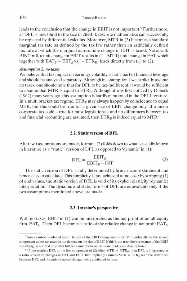
This in turn helps illustrating the dependence of wealth based DFLW on the choice of EBITB in exactly the same fashion as it is the case for the profit based DFL. Figure 3 is a wealth based version of figure 2. The switch from profit to wealth shifts the vertical asymptote to the left from EBITB = INT to EBITB = – E0 + INT (from EBITB = 5 to EBITB = –45 in our numerical example). DFL is greater than one for all values of EBITB if only the geared equity is not zero or negative.

Figure 3

Wealth based DFLW as a function of EBITB > –E0 + INT

0

2

4

6

8

10

12

14

–50 –30 –10 10 30

DFLW

EBITB



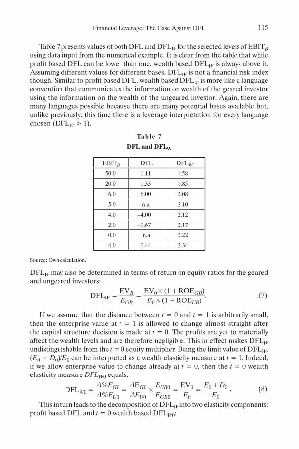
Table 7 presents values of both DFL and DFLW for the selected levels of EBITB using data input from the numerical example. It is clear from the table that while profit based DFL can be lower than one, wealth based DFLW is always above it. Assuming different values for different bases, DFLW is not a financial risk index though. Similar to profit based DFL, wealth based DFLW is more like a language convention that communicates the information on wealth of the geared investor using the information on the wealth of the ungeared investor. Again, there are many languages possible because there are many potential bases available but, unlike previously, this time there is a leverage interpretation for every language chosen (DFLW > 1).

Table 7DFL and DFLW

EBITB DFL DFLW

50.0 1.11 1.58

20.0 1.33 1.85

6.0 6.00 2.08

5.0 n.a. 2.10

4.0 –4.00 2.12

2.0 –0.67 2.17

0.0 n.a 2.22

–4.0 0.44 2.34


DFLW may also be determined in terms of return on equity ratios for the geared and ungeared investors:

.

.

.

%%

( )( )

( )( )

( )( )

%%

%%

(1 )( )

%%

( )( )

%%

,

( ) ( %)

( ) [ %]

*

( )( )

( )

( )

( )

( )

( )

( )

%%

( )( )

( )( )

DFLEBITEAT

EBIT EBITEAT EAT

EATEBIT

DFLEBIT INT

EBITETRMTR

EBIT EBITINT INT

DFLEBIT INT

EBIT

DFLEATEAT

EATEAT

EATEAT

DFLEV

DFLEV

EBIT INTEV EBIT

DFLEV

ROEEV ROE

DFLE EV

DFL DFL DFL

DFLEV EV

DFLEV

DFL DFL DFL

DFLX

X

EDFL

SEN

ELA

ELASEN

EE

EE

EE

EE D

EE

E

E E

E E

EE

E EE

E EE D

w w

E E kk

EE

EE

EE

E EE D

w w

Ek

E kE

Ek

E kE

E D

E

EE D

k w k w k

rr

N

r k

N

r k

NE

ENE

E E

NE

E ENE

E E

XY

XY

M

MEE

E kE k

kk

11

1

1

11

11 1

1

1 1

11

11

stdevstdev

i

B

B

B

B

B B

B

B B

B

B

B

U

G

U

G

GB

UB

WU

G

U

G

GB

UB

GB

UB

GB

B

WGB

B

B

B

WGB

B

UB

GB

WU

G

U

G

GB

UB

W W

WGB

B

G

U

WU

G

U

G

GB

UB

W W

W

U

U

U UU

G

G

G GG

G G U

U

G

Ui U

N

Gi Gi

N

UB

Ui UB

i

N

GB

Gi GB

i

N

UB

Ui UB

i

N

GB

Gi GB

i

N

W

UB

GB

UB U

GB G

U

G

0

0 0

0

0

0

0

00

0

0

0

0

0

0

0

0

0 0

1 0 2

0

0

00

0

0

0

0

0

0

0

0

0 0

1 0 2

0

00

0

00

1 2

2

2

02

2

02

2

2

2

2

2

0

0

# #

#

# #

#

#

#

# #

#

#

# #

# #

# # #

#

#

#

#

# #

!

D

D

D

D

D

D

D

D

D

D D

D

D

D

D

D

D

D

D

D

D

D

=- -

--

-

-

=-

= =

= = =+

=

= =+ -

+

= =+

+

= = = =+

= +

= =+

+

= +

=

+

+ +-

+

+ ++

-

=+

=

-

-

=-

-

-

-

=

=

=

= =+

+=

+

+

= =-

-

= = = =+

= +

=

= G

!

!

!

!

!

!

. (7)

If we assume that the distance between t = 0 and t = 1 is arbitrarily small, then the enterprise value at t = 1 is allowed to change almost straight after the capital structure decision is made at t = 0. The profits are yet to materially affect the wealth levels and are therefore negligible. This in effect makes DFLW undistinguishable from the t = 0 equity multiplier. Being the limit value of DFLW, (E0 + D0)/E0 can be interpreted as a wealth elasticity measure at t = 0. Indeed, if we allow enterprise value to change already at t = 0, then the t = 0 wealth elasticity measure DFLW0 equals:

.

.

.

%%

( )( )

( )( )

( )( )

%%

%%

(1 )( )

%%

( )( )

%%

,

( ) ( %)

( ) [ %]

*

( )( )

( )

( )

( )

( )

( )

( )

%%

( )( )

( )( )

DFLEBITEAT

EBIT EBITEAT EAT

EATEBIT

DFLEBIT INT

EBITETRMTR

EBIT EBITINT INT

DFLEBIT INT

EBIT

DFLEATEAT

EATEAT

EATEAT

DFLEV

DFLEV

EBIT INTEV EBIT

DFLEV

ROEEV ROE

DFLE EV

DFL DFL DFL

DFLEV EV

DFLEV

DFL DFL DFL

DFLX

X

EDFL

SEN

ELA

ELASEN

EE

EE

EE

EE D

EE

E

E E

E E

EE

E EE

E EE D

w w

E E kk

EE

EE

EE

E EE D

w w

Ek

E kE

Ek

E kE

E D

E

EE D

k w k w k

rr

N

r k

N

r k

NE

ENE

E E

NE

E ENE

E E

XY

XY

M

MEE

E kE k

kk

11

1

1

11

11 1

1

1 1

11

11

stdevstdev

i

B

B

B

B

B B

B

B B

B

B

B

U

G

U

G

GB

UB

WU

G

U

G

GB

UB

GB

UB

GB

B

WGB

B

B

B

WGB

B

UB

GB

WU

G

U

G

GB

UB

W W

WGB

B

G

U

WU

G

U

G

GB

UB

W W

W

U

U

U UU

G

G

G GG

G G U

U

G

Ui U

N

Gi Gi

N

UB

Ui UB

i

N

GB

Gi GB

i

N

UB

Ui UB

i

N

GB

Gi GB

i

N

W

UB

GB

UB U

GB G

U

G

0

0 0

0

0

0

0

00

0

0

0

0

0

0

0

0

0 0

1 0 2

0

0

00

0

0

0

0

0

0

0

0

0 0

1 0 2

0

00

0

00

1 2

2

2

02

2

02

2

2

2

2

2

0

0

# #

#

# #

#

#

#

# #

#

#

# #

# #

# # #

#

#

#

#

# #

!

D

D

D

D

D

D

D

D

D

D D

D

D

D

D

D

D

D

D

D

D

D

=- -

--

-

-

=-

= =

= = =+

=

= =+ -

+

= =+

+

= = = =+

= +

= =+

+

= +

=

+

+ +-

+

+ ++

-

=+

=

-

-

=-

-

-

-

=

=

=

= =+

+=

+

+

= =-

-

= = = =+

= +

=

= G

!

!

!

!

!

!

. (8)

This in turn leads to the decomposition of DFLW into two elasticity components: profit based DFL and t = 0 wealth based DFLW0:

Tomasz Berent116

.

.

.

%%

( )( )

( )( )

( )( )

%%

%%

(1 )( )

%%

( )( )

%%

,

( ) ( %)

( ) [ %]

*

( )( )

( )

( )

( )

( )

( )

( )

%%

( )( )

( )( )

DFLEBITEAT

EBIT EBITEAT EAT

EATEBIT

DFLEBIT INT

EBITETRMTR

EBIT EBITINT INT

DFLEBIT INT

EBIT

DFLEATEAT

EATEAT

EATEAT

DFLEV

DFLEV

EBIT INTEV EBIT

DFLEV

ROEEV ROE

DFLE EV

DFL DFL DFL

DFLEV EV

DFLEV

DFL DFL DFL

DFLX

X

EDFL

SEN

ELA

ELASEN

EE

EE

EE

EE D

EE

E

E E

E E

EE

E EE

E EE D

w w

E E kk

EE

EE

EE

E EE D

w w

Ek

E kE

Ek

E kE

E D

E

EE D

k w k w k

rr

N

r k

N

r k

NE

ENE

E E

NE

E ENE

E E

XY

XY

M

MEE

E kE k

kk

11

1

1

11

11 1

1

1 1

11

11

stdevstdev

i

B

B

B

B

B B

B

B B

B

B

B

U

G

U

G

GB

UB

WU

G

U

G

GB

UB

GB

UB

GB

B

WGB

B

B

B

WGB

B

UB

GB

WU

G

U

G

GB

UB

W W

WGB

B

G

U

WU

G

U

G

GB

UB

W W

W

U

U

U UU

G

G

G GG

G G U

U

G

Ui U

N

Gi Gi

N

UB

Ui UB

i

N

GB

Gi GB

i

N

UB

Ui UB

i

N

GB

Gi GB

i

N

W

UB

GB

UB U

GB G

U

G

0

0 0

0

0

0

0

00

0

0

0

0

0

0

0

0

0 0

1 0 2

0

0

00

0

0

0

0

0

0

0

0

0 0

1 0 2

0

00

0

00

1 2

2

2

02

2

02

2

2

2

2

2

0

0

# #

#

# #

#

#

#

# #

#

#

# #

# #

# # #

#

#

#

#

# #

!

D

D

D

D

D

D

D

D

D

D D

D

D

D

D

D

D

D

D

D

D

D

=- -

--

-

-

=-

= =

= = =+

=

= =+ -

+

= =+

+

= = = =+

= +

= =+

+

= +

=

+

+ +-

+

+ ++

-

=+

=

-

-

=-

-

-

-

=

=

=

= =+

+=

+

+

= =-

-

= = = =+

= +

=

= G

!

!

!

!

!

!

. (9)

with the weights w1 = E0/EBG and w2 = eATGB/eBG being determined by the extent to which initial equity capital and base profits of the geared investor contribute to his base wealth at t = 1.11

Equation (9) shows that profit based DFL is a mere component of wealth based DFLW. In studying financial leverage, wealth should be preferred to the wealth change, i.e. profit perspective because not only it excludes cases where DFL < 1 but it also seems to offer, as suggested in (9), a more comprehensive framework in which profit based DFL is a mere component.

4.2. Book vs. market values

market values of wealth provide a much better insight into actual investors’ utility than that offered by book values. more importantly, market value driven DFLW might offer the solution to the multiple value problem of DFL – still present in wealth driven DFLW. In contrast to book values, market value expected wealth, via expected/required rate of returns, determined by valuation equilibrium models such as CAPM or APT, has a clear and well-established meaning in finance. Each project is characterized by its (systematic) risk that is to be rewarded by the expected/required rate of return, kU and kG for the ungeared and geared investor respectively. The expected levels of market equity value for the ungeared and geared investors, against which percentage changes are calculated, amount to EUB = E0×(1 + kU) and EGB = E0×(1 + kG) respectively.

Let us assume that the numbers introduced in the numerical example above are market rather than book values: invested capital of 100 becomes now market enterprise value at t = 0, equity and debt levels of 50 are now market values at t = 0, hence D0/E0 = 1 denotes a market value debt-to-equity ratio at t = 0. If in our example kU = 20% and kG = 30%, with cost of debt of 10%, then DFLW is 1.85.12 Any percentage change in EU beyond the level that is determined by the systematic risk results in a levered (1.85 times greater in the numerical example) reaction in the equity value for the geared investor.

Equations (7)–(9) can also be presented in market value terms. DFLW in (10) turns to be a t = 1 market value equity multiplier with expected/required rates of return used as factors.

.

.

.

%%

( )( )

( )( )

( )( )

%%

%%

(1 )( )

%%

( )( )

%%

,

( ) ( %)

( ) [ %]

*

( )( )

( )

( )

( )

( )

( )

( )

%%

( )( )

( )( )

DFLEBITEAT

EBIT EBITEAT EAT

EATEBIT

DFLEBIT INT

EBITETRMTR

EBIT EBITINT INT

DFLEBIT INT

EBIT

DFLEATEAT

EATEAT

EATEAT

DFLEV

DFLEV

EBIT INTEV EBIT

DFLEV

ROEEV ROE

DFLE EV

DFL DFL DFL

DFLEV EV

DFLEV

DFL DFL DFL

DFLX

X

EDFL

SEN

ELA

ELASEN

EE

EE

EE

EE D

EE

E

E E

E E

EE

E EE

E EE D

w w

E E kk

EE

EE

EE

E EE D

w w

Ek

E kE

Ek

E kE

E D

E

EE D

k w k w k

rr

N

r k

N

r k

NE

ENE

E E

NE

E ENE

E E

XY

XY

M

MEE

E kE k

kk

11

1

1

11

11 1

1

1 1

11

11

stdevstdev

i

B

B

B

B

B B

B

B B

B

B

B

U

G

U

G

GB

UB

WU

G

U

G

GB

UB

GB

UB

GB

B

WGB

B

B

B

WGB

B

UB

GB

WU

G

U

G

GB

UB

W W

WGB

B

G

U

WU

G

U

G

GB

UB

W W

W

U

U

U UU

G

G

G GG

G G U

U

G

Ui U

N

Gi Gi

N

UB

Ui UB

i

N

GB

Gi GB

i

N

UB

Ui UB

i

N

GB

Gi GB

i

N

W

UB

GB

UB U

GB G

U

G

0

0 0

0

0

0

0

00

0

0

0

0

0

0

0

0

0 0

1 0 2

0

0

00

0

0

0

0

0

0

0

0

0 0

1 0 2

0

00

0

00

1 2

2

2

02

2

02

2

2

2

2

2

0

0

# #

#

# #

#

#

#

# #

#

#

# #

# #

# # #

#

#

#

#

# #

!

D

D

D

D

D

D

D

D

D

D D

D

D

D

D

D

D

D

D

D

D

D

=- -

--

-

-

=-

= =

= = =+

=

= =+ -

+

= =+

+

= = = =+

= +

= =+

+

= +

=

+

+ +-

+

+ ++

-

=+

=

-

-

=-

-

-

-

=

=

=

= =+

+=

+

+

= =-

-

= = = =+

= +

=

= G

!

!

!

!

!

!

. (10)

11 equation (9) can be useful in the analysis of the t = 1 wealth change when this change comes from the two distinct sources: t = 0 wealth and t = 1 profit.

12 See table 7 which can be regarded now as presenting market value DFLW with EBITB being replaced

by the enterprise (market) value expected/required change from t = 0 to t = 1.


on the other hand, the t = 0 market value equity multiplier can be interpreted as the elasticity measure if only market values are allowed to change at or straight after t = 0 (see equation (11)). should the investor experience an exogenous price shock (not related to the decision to gear or not to gear up) at t = 0 or at t = 1 arbitrarily close to t = 0, then the percentage change of the equity value for the geared investor is (E0 + D0)/E0 times greater than the percentage change experienced by the ungeared investor. needless to say, this is independent of both the direction and the size of the change:13

.

.

.

%%

( )( )

( )( )

( )( )

%%

%%

(1 )( )

%%

( )( )

%%

,

( ) ( %)

( ) [ %]

*

( )( )

( )

( )

( )

( )

( )

( )

%%

( )( )

( )( )

DFLEBITEAT

EBIT EBITEAT EAT

EATEBIT

DFLEBIT INT

EBITETRMTR

EBIT EBITINT INT

DFLEBIT INT

EBIT

DFLEATEAT

EATEAT

EATEAT

DFLEV

DFLEV

EBIT INTEV EBIT

DFLEV

ROEEV ROE

DFLE EV

DFL DFL DFL

DFLEV EV

DFLEV

DFL DFL DFL

DFLX

X

EDFL

SEN

ELA

ELASEN

EE

EE

EE

EE D

EE

E

E E

E E

EE

E EE

E EE D

w w

E E kk

EE

EE

EE

E EE D

w w

Ek

E kE

Ek

E kE

E D

E

EE D

k w k w k

rr

N

r k

N

r k

NE

ENE

E E

NE

E ENE

E E

XY

XY

M

MEE

E kE k

kk

11

1

1

11

11 1

1

1 1

11

11

stdevstdev

i

B

B

B

B

B B

B

B B

B

B

B

U

G

U

G

GB

UB

WU

G

U

G

GB

UB

GB

UB

GB

B

WGB

B

B

B

WGB

B

UB

GB

WU

G

U

G

GB

UB

W W

WGB

B

G

U

WU

G

U

G

GB

UB

W W

W

U

U

U UU

G

G

G GG

G G U

U

G

Ui U

N

Gi Gi

N

UB

Ui UB

i

N

GB

Gi GB

i

N

UB

Ui UB

i

N

GB

Gi GB

i

N

W

UB

GB

UB U

GB G

U

G

0

0 0

0

0

0

0

00

0

0

0

0

0

0

0

0

0 0

1 0 2

0

0

00

0

0

0

0

0

0

0

0

0 0

1 0 2

0

00

0

00

1 2

2

2

02

2

02

2

2

2

2

2

0

0

# #

#

# #

#

#

#

# #

#

#

# #

# #

# # #

#

#

#

#

# #

!

D

D

D

D

D

D

D

D

D

D D

D

D

D

D

D

D

D

D

D

D

D

=- -

--

-

-

=-

= =

= = =+

=

= =+ -

+

= =+

+

= = = =+

= +

= =+

+

= +

=

+

+ +-

+

+ ++

-

=+

=

-

-

=-

-

-

-

=

=

=

= =+

+=

+

+

= =-

-

= = = =+

= +

=

= G

!

!

!

!

!

!

. (11)

Last but not least, market value based DFLW can be shown to be a weighted average of market value DFL and market value DFLW0:

.

.

.

%%

( )( )

( )( )

( )( )

%%

%%

(1 )( )

%%

( )( )

%%

,

( ) ( %)

( ) [ %]

*

( )( )

( )

( )

( )

( )

( )

( )

%%

( )( )

( )( )

DFLEBITEAT

EBIT EBITEAT EAT

EATEBIT

DFLEBIT INT

EBITETRMTR

EBIT EBITINT INT

DFLEBIT INT

EBIT

DFLEATEAT

EATEAT

EATEAT

DFLEV

DFLEV

EBIT INTEV EBIT

DFLEV

ROEEV ROE

DFLE EV

DFL DFL DFL

DFLEV EV

DFLEV

DFL DFL DFL

DFLX

X

EDFL

SEN

ELA

ELASEN

EE

EE

EE

EE D

EE

E

E E

E E

EE

E EE

E EE D

w w

E E kk

EE

EE

EE

E EE D

w w

Ek

E kE

Ek

E kE

E D

E

EE D

k w k w k

rr

N

r k

N

r k

NE

ENE

E E

NE

E ENE

E E

XY

XY

M

MEE

E kE k

kk

11

1

1

11

11 1

1

1 1

11

11

stdevstdev

i

B

B

B

B

B B

B

B B

B

B

B

U

G

U

G

GB

UB

WU

G

U

G

GB

UB

GB

UB

GB

B

WGB

B

B

B

WGB

B

UB

GB

WU

G

U

G

GB

UB

W W

WGB

B

G

U

WU

G

U

G

GB

UB

W W

W

U

U

U UU

G

G

G GG

G G U

U

G

Ui U

N

Gi Gi

N

UB

Ui UB

i

N

GB

Gi GB

i

N

UB

Ui UB

i

N

GB

Gi GB

i

N

W

UB

GB

UB U

GB G

U

G

0

0 0

0

0

0

0

00

0

0

0

0

0

0

0

0

0 0

1 0 2

0

0

00

0

0

0

0

0

0

0

0

0 0

1 0 2

0

00

0

00

1 2

2

2

02

2

02

2

2

2

2

2

0

0

# #

#

# #

#

#

#

# #

#

#

# #

# #

# # #

#

#

#

#

# #

!

D

D

D

D

D

D

D

D

D

D D

D

D

D

D

D

D

D

D

D

D

D

=- -

--

-

-

=-

= =

= = =+

=

= =+ -

+

= =+

+

= = = =+

= +

= =+

+

= +

=

+

+ +-

+

+ ++

-

=+

=

-

-

=-

-

-

-

=

=

=

= =+

+=

+

+

= =-

-

= = = =+

= +

=

= G

!

!

!

!

!

!

, (12)

with the weights w1 = E0/EGB and w2 = eATGB/EGB being determined by the extent to which initial equity capital of the geared investor and its expected change contribute to his market value base wealth at t = 1.

To summarize, market value driven DFLW is not only greater than one and relevant to decision makers but it also offers a clear-cut base for the elasticity analysis. With an obvious benchmark candidate, the multiple value problem of DFL vanishes altogether. The last question to be addressed is the very meaning of this unique value of DFLW, 1.85 in our numerical example. Is it really what Markowitz and Sharpe meant when they wrote on financial risk?

4.3. DFLW as a downward biased estimator

The elasticity analysis presented above is performed from the ‘cum wealth change from t = 0 to t = 1’ perspective. This is the legacy of where we have started, i.e. the elasticity analysis based on profit reported at t = 1. DFLW happens to be a t = 1 equity multiplier (E + D)/D, equal to 1.85 in our numerical example. However, it is a t = 0 equity multiplier (E0 + D0)/E0, equal to 2.0 in our example, that is the measure of financial leverage as understood by both Markowitz and Sharpe. Both the standard deviation of the geared equity in the context of the Capital market Line as well as the equity beta in the context of the security market Line get magnified in the absence of bankruptcy risk by factor (E0 + D0)/E0. This is shown, among others, by seminal work of Hamada (1972) and Rubinstein (1973).

13 Although equations (10)–(12) are defined for the expected values of wealth, one can easily present them in the form of any size of wealth change from t = 0 to t = 1. If so, the multiple value problem of DFL and the language convention interpretation are still relevant.

Tomasz Berent118

Consequently, this is the t = 0 equity multiplier that describes the actual risk exposure of the geared versus ungeared investor, not a t = 1 ratio.

Adopting the investor’s perspective really helps see it more clearly. The shareholder who invites a co-owner, invites someone who does share his fortunes in good and misfortunes in bad times: the joy of being above the expected level of wealth, given the inherent risk, and disappointment of being below it. The ungeared investor participates only in a fraction E0/(D0 + E0) < 1 of the deviation from the expected wealth level, while the geared investor takes the whole deviation himself. In other words, the geared investor’s change in wealth is always (D0 + E0)/E0 times bigger than that for the ungeared investor. The point is that the changes here are real money, denominated in currency units - any swing in enterprise value translates immediately into the value of equity positions. And it is a t = 1 equity multiplier, determined by the size of the external funding at t = 0, that quantifies the difference in wealth reaction of the geared and ungeared investors.

Being a t = 1 market value equity multiplier, a wealth based DFLW is bound to be a downward biased estimator of the true financial leverage measure. This is already indicated by (10), with kU being by definition lower than kG. Below we attempt to illustrate in detail the roots of this downward bias.

Firstly, DFLW can be shown to have implicitly incorporated a wrong discount rate. To see this, we present the decomposition of DFLW in which the index is expressed as the ratio of relative wealth changes using present values of t = 1 equity levels. This approach is particularly appealing if one assumes that the information relating to the change in equity value at t = 1 is already available at t = 0 and that capital markets are efficient in the sense similar to the way proposed by Fama. As shown below, DFLW uses kG as an implied discount rate (circled in 13):

.

.

.

%%

( )( )

( )( )

( )( )

%%

%%

(1 )( )

%%

( )( )

%%

,

( ) ( %)

( ) [ %]

*

( )( )

( )

( )

( )

( )

( )

( )

%%

( )( )

( )( )

DFLEBITEAT

EBIT EBITEAT EAT

EATEBIT

DFLEBIT INT

EBITETRMTR

EBIT EBITINT INT

DFLEBIT INT

EBIT

DFLEATEAT

EATEAT

EATEAT

DFLEV

DFLEV

EBIT INTEV EBIT

DFLEV

ROEEV ROE

DFLE EV

DFL DFL DFL

DFLEV EV

DFLEV

DFL DFL DFL

DFLX

X

EDFL

SEN

ELA

ELASEN

EE

EE

EE

EE D

EE

E

E E

E E

EE

E EE

E EE D

w w

E E kk

EE

EE

EE

E EE D

w w

Ek

E kE

Ek

E kE

E D

E

EE D

k w k w k

rr

N

r k

N

r k

NE

ENE

E E

NE

E ENE

E E

XY

XY

M

MEE

E kE k

kk

11

1

1

11

11 1

1

1 1

11

11

stdevstdev

i

B

B

B

B

B B

B

B B

B

B

B

U

G

U

G

GB

UB

WU

G

U

G

GB

UB

GB

UB

GB

B

WGB

B

B

B

WGB

B

UB

GB

WU

G

U

G

GB

UB

W W

WGB

B

G

U

WU

G

U

G

GB

UB

W W

W

U

U

U UU

G

G

G GG

G G U

U

G

Ui U

N

Gi Gi

N

UB

Ui UB

i

N

GB

Gi GB

i

N

UB

Ui UB

i

N

GB

Gi GB

i

N

W

UB

GB

UB U

GB G

U

G

0

0 0

0

0

0

0

00

0

0

0

0

0

0

0

0

0 0

1 0 2

0

0

00

0

0

0

0

0

0

0

0

0 0

1 0 2

0

00

0

00

1 2

2

2

02

2

02

2

2

2

2

2

0

0

# #

#

# #

#

#

#

# #

#

#

# #

# #

# # #

#

#

#

#

# #

!

D

D

D

D

D

D

D

D

D

D D

D

D

D

D

D

D

D

D

D

D

D

=- -

--

-

-

=-

= =

= = =+

=

= =+ -

+

= =+

+

= = = =+

= +

= =+

+

= +

=

+

+ +-

+

+ ++

-

=+

=

-

-

=-

-

-

-

=

=

=

= =+

+=

+

+

= =-

-

= = = =+

= +

=

= G

!

!

!

!

!

!

. (13)

However, this rate is wrong: too large if the deviation from the expected value at t = 1 is positive and too small if the deviation is negative. If the company’s valuation is likely to be X% above the expected level of kU, and the markets incorporate this information instantaneously at t = 0, then the value of equity grows already at t = 0. A debt-to-equity ratio goes down reducing the financial risk as a result. Consequently, the rate required by the geared investor falls below kG. Conversely, if X% < 0, then the financial risk of the geared investor’s increases and kG is too small. In either case, using a wrong discount rate results in DFLW being a downward biased estimator of DFLW0 for X% ! 0.


should the correct discount rate k*G be used, the ratio in (13) would have

equalled (E0 + D0)/E0 rather than (E + D)/E. The correct discount rate k*G can

be shown to be a weighted average of kG and kU:14

k*

G

.

.

.

%%

( )( )

( )( )

( )( )

%%

%%

(1 )( )

%%

( )( )

%%

,

( ) ( %)

( ) [ %]

*

( )( )

( )

( )

( )

( )

( )

( )

%%

( )( )

( )( )

DFLEBITEAT

EBIT EBITEAT EAT

EATEBIT

DFLEBIT INT

EBITETRMTR

EBIT EBITINT INT

DFLEBIT INT

EBIT

DFLEATEAT

EATEAT

EATEAT

DFLEV

DFLEV

EBIT INTEV EBIT

DFLEV

ROEEV ROE

DFLE EV

DFL DFL DFL

DFLEV EV

DFLEV

DFL DFL DFL

DFLX

X

EDFL

SEN

ELA

ELASEN

EE

EE

EE

EE D

EE

E

E E

E E

EE

E EE

E EE D

w w

E E kk

EE

EE

EE

E EE D

w w

Ek

E kE

Ek

E kE

E D

E

EE D

k w k w k

rr

N

r k

N

r k

NE

ENE

E E

NE

E ENE

E E

XY

XY

M

MEE

E kE k

kk

11

1

1

11

11 1

1

1 1

11

11

stdevstdev

i

B

B

B

B

B B

B

B B

B

B

B

U

G

U

G

GB

UB

WU

G

U

G

GB

UB

GB

UB

GB

B

WGB

B

B

B

WGB

B

UB

GB

WU

G

U

G

GB

UB

W W

WGB

B

G

U

WU

G

U

G

GB

UB

W W

W

U

U

U UU

G

G

G GG

G G U

U

G

Ui U

N

Gi Gi

N

UB

Ui UB

i

N

GB

Gi GB

i

N

UB

Ui UB

i

N

GB

Gi GB

i

N

W

UB

GB

UB U

GB G

U

G

0

0 0

0

0

0

0

00

0

0

0

0

0

0

0

0

0 0

1 0 2

0

0

00

0

0

0

0

0

0

0

0

0 0

1 0 2

0

00

0

00

1 2

2

2

02

2

02

2

2

2

2

2

0

0

# #

#

# #

#

#

#

# #

#

#

# #

# #

# # #

#

#

#

#

# #

!

D

D

D

D

D

D

D

D

D

D D

D

D

D

D

D

D

D

D

D

D

D

=- -

--

-

-

=-

= =

= = =+

=

= =+ -

+

= =+

+

= = = =+

= +

= =+

+

= +

=

+

+ +-

+

+ ++

-

=+

=

-

-

=-

-

-

-

=

=

=

= =+

+=

+

+

= =-

-

= = = =+

= +

=

= G

!

!

!

!

!

!

, (14)

where

w1 = 1/[1 + (E0 + D0)/E0)×X%] > 0

and

w2 = [(E0 + D0)/E0×X%]/[1 + (E0 + D0)/E0)×X%] < 1.

one can verify that if X% > 0 then k*G < kG, if X% < 0 then k*

G > kG. remember, we assume X% > –100%/[(E0 + D0)/E0] to secure positive values of geared equity.

We now demonstrate that DFLW, although different from the t = 0 equity multiplier, does inconspicuously resemble the ratio of standard deviations of returns generated by the geared and ungeared investors. This ratio equals (E0 + D0)/E0. If properly readjusted, DFLW can be shown to be:

.

.

.

%%

( )( )

( )( )

( )( )

%%

%%

(1 )( )

%%

( )( )

%%

,

( ) ( %)

( ) [ %]

*

( )( )

( )

( )

( )

( )

( )

( )

%%

( )( )

( )( )

DFLEBITEAT

EBIT EBITEAT EAT

EATEBIT

DFLEBIT INT

EBITETRMTR

EBIT EBITINT INT

DFLEBIT INT

EBIT

DFLEATEAT

EATEAT

EATEAT

DFLEV

DFLEV

EBIT INTEV EBIT

DFLEV

ROEEV ROE

DFLE EV

DFL DFL DFL

DFLEV EV

DFLEV

DFL DFL DFL

DFLX

X

EDFL

SEN

ELA

ELASEN

EE

EE

EE

EE D

EE

E

E E

E E

EE

E EE

E EE D

w w

E E kk

EE

EE

EE

E EE D

w w

Ek

E kE

Ek

E kE

E D

E

EE D

k w k w k

rr

N

r k

N

r k

NE

ENE

E E

NE

E ENE

E E

XY

XY

M

MEE

E kE k

kk

11

1

1

11

11 1

1

1 1

11

11

stdevstdev

i

B

B

B

B

B B

B

B B

B

B

B

U

G

U

G

GB

UB

WU

G

U

G

GB

UB

GB

UB

GB

B

WGB

B

B

B

WGB

B

UB

GB

WU

G

U

G

GB

UB

W W

WGB

B

G

U

WU

G

U

G

GB

UB

W W

W

U

U

U UU

G

G

G GG

G G U

U

G

Ui U

N

Gi Gi

N

UB

Ui UB

i

N

GB

Gi GB

i

N

UB

Ui UB

i

N

GB

Gi GB

i

N

W

UB

GB

UB U

GB G

U

G

0

0 0

0

0

0

0

00

0

0

0

0

0

0

0

0

0 0

1 0 2

0

0

00

0

0

0

0

0

0

0

0

0 0

1 0 2

0

00

0

00

1 2

2

2

02

2

02

2

2

2

2

2

0

0

# #

#

# #

#

#

#

# #

#

#

# #

# #

# # #

#

#

#

#

# #

!

D

D

D

D

D

D

D

D

D

D D

D

D

D

D

D

D

D

D

D

D

D

=- -

--

-

-

=-

= =

= = =+

=

= =+ -

+

= =+

+

= = = =+

= +

= =+

+

= +

=

+

+ +-

+

+ ++

-

=+

=

-

-

=-

-

-

-

=

=

=

= =+

+=

+

+

= =-

-

= = = =+

= +

=

= G

!

!

!

!

!

!

(15)

The ratio of standard deviations in (15) features identical t = 0 equity levels EGB0 and EUB0. They cancel out as a result, so effectively the ratio becomes the ratio of absolute differences between wealth levels and the base, i.e. (EGi – EGB)/(EUi – EUB).15 In contrast, DFLW features t = 1 equity levels EGB and EUB that are all but identical. These levels include the expected/required reward for the risk taken that makes EGB greater than EUB. no surprise, after all DFLW is but a ratio of relative rather than absolute differences between wealth levels and the base, i.e. [(EGi – EGB)/EGB]/[(EUi – EUB)/EUB].

As the t = 1 bases incorporate the expected/required reward for the risk taken between t = 0 and t = 1, DFL is simply a bundle of risk taken and at the same time the reward for this risk. We believe this is misleading or even outright wrong if DFL is supposed to be a risk measure alone.

14 E*G, the geared investor equity value at t = 1 that corresponds to the ungeared equity value that at t

= 1 is X% above/below its expected level, equals: E*G = [E0 ×(1 + kG)] × [1 + (E + D)/E × X%]. Alter-X%]. Alter-%]. Alter-

natively, it is the future value of E0 × [1 + (E0 + D0)/E0 × X%] compounded at k*G. This leads to equation

(14). 15 note that, since EG is a linear function of EU, the square root and power two in (15) do cancel out.

Tomasz Berent120

similar conclusions can be reached from the inspection of equation (12), where DFLW is portrayed as the weighted average of DFLW0 = (E0 + D0)/E0 and DFL. If w2 = kG×EGB0 is zero, an assumption justified if t = 1 is arbitrarily close to t = 0, and consequently kG becomes arbitrarily close to zero, then DFLW approaches DFLW0 = (E0 + D0)/E0. However, the weight of DFL in (12) is not zero and hence DFLW remains dependent on the t = 1 risk reward inherent in DFL.

Indeed, if by attaching all the weight in (12) to w1 we could turn a blind eye to the fact that DFLW is a t = 1 rather than t = 0 elasticity measure, then we end up with a t = 0 equity multiplier, just like in the work of markowitz and sharpe. The question being addressed by a t = 0 elasticity analysis is about the extent to which any immediate potential change in market valuation of the ungeared investor gets levered for the geared investor. Although the question is certainly about financial leverage and relevant for those contemplating taking debt, and it leads to the answer in line with the analysis of markowitz and sharpe, the differences between this result and that obtained by Markowitz and Sharpe are still significant. As the focus is now shifted to t = 0, there is no mention about expected returns, variances, and betas – all calculated in t = 1 and as such indispensable in markowitz and sharpe work.

The rationale behind the switch from a t = 1 to t = 0 framework is primarily to protect the elasticity interpretation of DFL – arguably single most characteristic feature of DFL. Yet as shown in (15) and alluded to earlier in the section on investor’s perspective, it is the sensitivity index, i.e. a measure of absolute’s changes in the wealth levels, rather than the elasticity index, i.e. the ratio of relative changes, that captures the essence of the financial leverage risk. Note, this sensitivity measure amounts to (E0 + D0)/E0 as suggested by markowitz and Sharpe. If we are to keep a t = 1 perspective, we must switch from the elasticity towards sensitivity analysis. But how can a t = 0 equity multiplier (E0 + D0)/E0 be a t = 0 elasticity measure (see equations 11–12) and at the same time a t = 1 sensitivity index? The answer is explained below.

Let us define a sensitivity SEN and elasticity ELA measures for a pair of any two variables Y and X as the ratio of their absolute and relative changes respectively:

.

.

.

%%

( )( )

( )( )

( )( )

%%

%%

(1 )( )

%%

( )( )

%%

,

( ) ( %)

( ) [ %]

*

( )( )

( )

( )

( )

( )

( )

( )

%%

( )( )

( )( )

DFLEBITEAT

EBIT EBITEAT EAT

EATEBIT

DFLEBIT INT

EBITETRMTR

EBIT EBITINT INT

DFLEBIT INT

EBIT

DFLEATEAT

EATEAT

EATEAT

DFLEV

DFLEV

EBIT INTEV EBIT

DFLEV

ROEEV ROE

DFLE EV

DFL DFL DFL

DFLEV EV

DFLEV

DFL DFL DFL

DFLX

X

EDFL

SEN

ELA

ELASEN

EE

EE

EE

EE D

EE

E

E E

E E

EE

E EE

E EE D

w w

E E kk

EE

EE

EE

E EE D

w w

Ek

E kE

Ek

E kE

E D

E

EE D

k w k w k

rr

N

r k

N

r k

NE

ENE

E E

NE

E ENE

E E

XY

XY

M

MEE

E kE k

kk

11

1

1

11

11 1

1

1 1

11

11

stdevstdev

i

B

B

B

B

B B

B

B B

B

B

B

U

G

U

G

GB

UB

WU

G

U

G

GB

UB

GB

UB

GB

B

WGB

B

B

B

WGB

B

UB

GB

WU

G

U

G

GB

UB

W W

WGB

B

G

U

WU

G

U

G

GB

UB

W W

W

U

U

U UU

G

G

G GG

G G U

U

G

Ui U

N

Gi Gi

N

UB

Ui UB

i

N

GB

Gi GB

i

N

UB

Ui UB

i

N

GB

Gi GB

i

N

W

UB

GB

UB U

GB G

U

G

0

0 0

0

0

0

0

00

0

0

0

0

0

0

0

0

0 0

1 0 2

0

0

00

0

0

0

0

0

0

0

0

0 0

1 0 2

0

00

0

00

1 2

2

2

02

2

02

2

2

2

2

2

0

0

# #

#

# #

#

#

#

# #

#

#

# #

# #

# # #

#

#

#

#

# #

!

D

D

D

D

D

D

D

D

D

D D

D

D

D

D

D

D

D

D

D

D

D

=- -

--

-

-

=-

= =

= = =+

=

= =+ -

+

= =+

+

= = = =+

= +

= =+

+

= +

=

+

+ +-

+

+ ++

-

=+

=

-

-

=-

-

-

-

=

=

=

= =+

+=

+

+

= =-

-

= = = =+

= +

=

= G

!

!

!

!

!

!

, (16)

.

.

.

%%

( )( )

( )( )

( )( )

%%

%%

(1 )( )

%%

( )( )

%%

,

( ) ( %)

( ) [ %]

*

( )( )

( )

( )

( )

( )

( )

( )

%%

( )( )

( )( )

DFLEBITEAT

EBIT EBITEAT EAT

EATEBIT

DFLEBIT INT

EBITETRMTR

EBIT EBITINT INT

DFLEBIT INT

EBIT

DFLEATEAT

EATEAT

EATEAT

DFLEV

DFLEV

EBIT INTEV EBIT

DFLEV

ROEEV ROE

DFLE EV

DFL DFL DFL

DFLEV EV

DFLEV

DFL DFL DFL

DFLX

X

EDFL

SEN

ELA

ELASEN

EE

EE

EE

EE D

EE

E

E E

E E

EE

E EE

E EE D

w w

E E kk

EE

EE

EE

E EE D

w w

Ek

E kE

Ek

E kE

E D

E

EE D

k w k w k

rr

N

r k

N

r k

NE

ENE

E E

NE

E ENE

E E

XY

XY

M

MEE

E kE k

kk

11

1

1

11

11 1

1

1 1

11

11

stdevstdev

i

B

B

B

B

B B

B

B B

B

B

B

U

G

U

G

GB

UB

WU

G

U

G

GB

UB

GB

UB

GB

B

WGB

B

B

B

WGB

B

UB

GB

WU

G

U

G

GB

UB

W W

WGB

B

G

U

WU

G

U

G

GB

UB

W W

W

U

U

U UU

G

G

G GG

G G U

U

G

Ui U

N

Gi Gi

N

UB

Ui UB

i

N

GB

Gi GB

i

N

UB

Ui UB

i

N

GB

Gi GB

i

N

W

UB

GB

UB U

GB G

U

G

0

0 0

0

0

0

0

00

0

0

0

0

0

0

0

0

0 0

1 0 2

0

0

00

0

0

0

0

0

0

0

0

0 0

1 0 2

0

00

0

00

1 2

2

2

02

2

02

2

2

2

2

2

0

0

# #

#

# #

#

#

#

# #

#

#

# #

# #

# # #

#

#

#

#

# #

!

D

D

D

D

D

D

D

D

D

D D

D

D

D

D

D

D

D

D

D

D

D

=- -

--

-

-

=-

= =

= = =+

=

= =+ -

+

= =+

+

= = = =+

= +

= =+

+

= +

=

+

+ +-

+

+ ++

-

=+

=

-

-

=-

-

-

-

=

=

=

= =+

+=

+

+

= =-

-

= = = =+

= +

=

= G

!

!

!

!

!

!

. (17)

Then it is rather trivial to see that regardless of the functional relationship between Y and X, the elasticity measure eLA is a ratio of the sensitivity measure sen and the multiplier M = YB/XB of the base values against which percentage changes are calculated in eLA:

.

.

.

%%

( )( )

( )( )

( )( )

%%

%%

(1 )( )

%%

( )( )

%%

,

( ) ( %)

( ) [ %]

*

( )( )

( )

( )

( )

( )

( )

( )

%%

( )( )

( )( )

DFLEBITEAT

EBIT EBITEAT EAT

EATEBIT

DFLEBIT INT

EBITETRMTR

EBIT EBITINT INT

DFLEBIT INT

EBIT

DFLEATEAT

EATEAT

EATEAT

DFLEV

DFLEV

EBIT INTEV EBIT

DFLEV

ROEEV ROE

DFLE EV

DFL DFL DFL

DFLEV EV

DFLEV

DFL DFL DFL

DFLX

X

EDFL

SEN

ELA

ELASEN

EE

EE

EE

EE D

EE

E

E E

E E

EE

E EE

E EE D

w w

E E kk

EE

EE

EE

E EE D

w w

Ek

E kE

Ek

E kE

E D

E

EE D

k w k w k

rr

N

r k

N

r k

NE

ENE

E E

NE

E ENE

E E

XY

XY

M

MEE

E kE k

kk

11

1

1

11

11 1

1

1 1

11

11

stdevstdev

i

B

B

B

B

B B

B

B B

B

B

B

U

G

U

G

GB

UB

WU

G

U

G

GB

UB

GB

UB

GB

B

WGB

B

B

B

WGB

B

UB

GB

WU

G

U

G

GB

UB

W W

WGB

B

G

U

WU

G

U

G

GB

UB

W W

W

U

U

U UU

G

G

G GG

G G U

U

G

Ui U

N

Gi Gi

N

UB

Ui UB

i

N

GB

Gi GB

i

N

UB

Ui UB

i

N

GB

Gi GB

i

N

W

UB

GB

UB U

GB G

U

G

0

0 0

0

0

0

0

00

0

0

0

0

0

0

0

0

0 0

1 0 2

0

0

00

0

0

0

0

0

0

0

0

0 0

1 0 2

0

00

0

00

1 2

2

2

02

2

02

2

2

2

2

2

0

0

# #

#

# #

#

#

#

# #

#

#

# #

# #

# # #

#

#

#

#

# #

!

D

D

D

D

D

D

D

D

D

D D

D

D

D

D

D

D

D

D

D

D

D

=- -

--

-

-

=-

= =

= = =+

=

= =+ -

+

= =+

+

= = = =+

= +

= =+

+

= +

=

+

+ +-

+

+ ++

-

=+

=

-

-

=-

-

-

-

=

=

=

= =+

+=

+

+

= =-

-

= = = =+

= +

=

= G

!

!

!

!

!

!

. (18)


At t = 0, the wealth bases for the geared and ungeared investors are identical and hence M = 1. It follows from (18) that as SEN is always equal to (E0 + D0)/E0 then also eLA = (E0 + D0)/E0 at t = 0. The sensitivity ratio is constant across time as the geared investor absorbs always the whole (unexpected) enterprise value change, while the ungeared one takes only a fraction of it, determined by his share in total equity, i.e. E0/(E0 + D0). Consequently, it should be no surprise that the t = 0 elasticity index is identical to the t = 1 sensitivity measure.

To sum up, the reason why the elasticity analysis when performed at t = 0 produces identical results with the analysis of markowitz and sharpe, clearly determined by sensitivity analysis at t = 1, is that the elasticity index at t = 0 becomes indistinguishable from the sensitivity index at t = 0 and subsequently from the sensitivity index at t = 1.

As the wealth based multiplier M is greater than one at t = 1, it is not surprising that DFLW being an elasticity index is a downward biased estimator of (E0 + D0)/E0 (see (18)). To remove the bias we must multiply DFLW = (E + D)/E by the wealth base multiplier M:

.

.

.

%%

( )( )

( )( )

( )( )

%%

%%

(1 )( )

%%

( )( )

%%

,

( ) ( %)

( ) [ %]

*

( )( )

( )

( )

( )

( )

( )

( )

%%

( )( )

( )( )

DFLEBITEAT

EBIT EBITEAT EAT

EATEBIT

DFLEBIT INT

EBITETRMTR

EBIT EBITINT INT

DFLEBIT INT

EBIT

DFLEATEAT

EATEAT

EATEAT

DFLEV

DFLEV

EBIT INTEV EBIT

DFLEV

ROEEV ROE

DFLE EV

DFL DFL DFL

DFLEV EV

DFLEV

DFL DFL DFL

DFLX

X

EDFL

SEN

ELA

ELASEN

EE

EE

EE

EE D

EE

E

E E

E E

EE

E EE

E EE D

w w

E E kk

EE

EE

EE

E EE D

w w

Ek

E kE

Ek

E kE

E D

E

EE D

k w k w k

rr

N

r k

N

r k

NE

ENE

E E

NE

E ENE

E E

XY

XY

M

MEE

E kE k

kk

11

1

1

11

11 1

1

1 1

11

11

stdevstdev

i

B

B

B

B

B B

B

B B

B

B

B

U

G

U

G

GB

UB

WU

G

U

G

GB

UB

GB

UB

GB

B

WGB

B

B

B

WGB

B

UB

GB

WU

G

U

G

GB

UB

W W

WGB

B

G

U

WU

G

U

G

GB

UB

W W

W

U

U

U UU

G

G

G GG

G G U

U

G

Ui U

N

Gi Gi

N

UB

Ui UB

i

N

GB

Gi GB

i

N

UB

Ui UB

i

N

GB

Gi GB

i

N

W

UB

GB

UB U

GB G

U

G

0

0 0

0

0

0

0

00

0

0

0

0

0

0

0

0

0 0

1 0 2

0

0

00

0

0

0

0

0

0

0

0

0 0

1 0 2

0

00

0

00

1 2

2

2

02

2

02

2

2

2

2

2

0

0

# #

#

# #

#

#

#

# #

#

#

# #

# #

# # #

#

#

#

#

# #

!

D

D

D

D

D

D

D

D

D

D D

D

D

D

D

D

D

D

D

D

D

D

=- -

--

-

-

=-

= =

= = =+

=

= =+ -

+

= =+

+

= = = =+

= +

= =+

+

= +

=

+

+ +-

+

+ ++

-

=+

=

-

-

=-

-

-

-

=

=

=

= =+

+=

+

+

= =-

-

= = = =+

= +

=

= G

!

!

!

!

!

!

. (19)

Based on equation (10) it is easy to see that what we end up with is the desired equity multiplier at t = 0.

If one wants to phrase the implications of taking debt in the form of a leverage narrative with financial leverage index amounting to (E0 + D0)/E0, one needs to either switch the elasticity analysis from t = 1 to t = 0 or switch the analysis away from the elasticity towards the sensitivity study at t = 1; the latter is what markowitz and sharpe did. Any attempt to retain the elasticity analysis at t = 1 results in either the loss of the leverage interpretation or, if leverage interpretation is available and expected value of t = 1 wealth is used as a base, in a distorted, downward biased risk estimator.

Paradoxically, equation (18) does also suggest that the whole journey from the classic profit based DFL via wealth (first book then market value) based DFLW up until the one unique level of DFLW determined for the expected market equity value at t = 1 may not have been necessary in the first place. Thanks to (18), the information on the unbiased estimator of the financial leverage risk can be retrieved from any biased estimator, not necessarily the one calculated so studiously for the expected level of equity. Any market value DFL, calculated for wealth or wealth change, greater than one, a fraction or even a negative number, leads according to (18) to the same sensitivity ratio, i.e. (D0 + E0)/E0. returning to the language convention theme, although market value wealth perspective offers one unique and unambiguous language to communicate various business outcomes, it still needs, as an elasticity index, decoding using (18) to present a true financial leverage risk story, accurately captured only by the sensitivity index. If this is so, we may easily live up with any language whatsoever, regardless of how difficult and unintuitive it is in usage, with or without leverage interpretation, as

Tomasz Berent122

long as we know how to decode it. The only thing we need is the key to the code, i.e. the base multiplier to be used in (18).

note, one may even ask why to learn how to decode the encoded information if the information on the t = 0 equity multiplier, a true leverage risk indicator, is readily available! This begs a question “why to calculate DFL at all?”.

Conclusions

The degree of financial leverage DFL is a well-established financial analysis index that is supposed to capture the size of financial leverage risk. When greater than one, it points to the more than proportional relative change in net profit compared to the corresponding relative change in operating profit. We believe that it is its elasticity interpretation that has made DFL so popular in the financial literature even if its origins, rooted in managerial accounting and financial analysis, areas populated with concepts such as break-even points, profit margins etc., are well away from the finance theory field preoccupied with notions such as risk-reward trade off, cost of capital and valuation.

Unfortunately, the standard definition of DFL makes even the start of the analytical work difficult. It is claimed in this paper that only after making additional assumptions, DFL – re-expressed now from the perspective of an investor rather than that of a company - does unambiguously refer to a given leverage state and is immune to both changes in tax regimes and the size of profit change analysed. The initial verdict on the usefulness of DFL must be negative if only because the index is phrased in accounting terms and focused on merely one year profit. As a result DFL can barely claim to be of much relevance to practice interested in market values and wealth rather than profit.

To make it worse, in contrast to neatly presented numerical examples in textbooks, DFL may produce values that are not greater than one, so its financial leverage credentials are dubious too. Failure to distinguish between risk and risk reward dimensions, bundled together into one measure, is unfortunate. DFL seems to be all but the measure of the greater variability of prospective rates of returns to leveraged shareholders or the measure of greater financial risk of markowitz and sharpe as it was claimed by merton miller in his nobel memorial Prize Lecture.

DFL’s fatal flaw is that it is the ratio of relative rather than absolute changes at t = 1. This makes DFL an index that tells us more about the (usually arbitrary) choice of the profit base against which relative changes are measured than about financial risk caused by firm’s financial activity. Each base leads to a different value of DFL. As there are hardly any rules that govern the choice of the base, there is also little one can say about the validity of any given DFL. For this reason, we propose to view DFL more as a language convention than a financial risk


indicator. Within such a convention, frequently lacking leverage interpretation, a user chooses the profit base that subsequently determines DFL and by doing so determines the way various business outcomes are communicated to the outside world. There are many legitimate languages to communicate the same information, just like there are many legitimate bases, e.g. management forecast, market expectation or last year’s profits to choose from.

The scrutiny of constituent characteristics of DFL ultimately responsible for severe shortcomings of the index and its rather modest applicability among both practitioners and empirical researchers has led us to the process of a step-by-step modification of the measure. We have thus changed gradually from book to market values, from profit to wealth, and from future to current date perspective. At first we attempted to target all but one characteristic of DFL, its elasticity format – its allegedly most attractive and at the same time most controversial feature, yet the one that makes DFL what it is.

By moving from the profit to wealth perspective, we replace a standard profit based DFL with wealth based DFLW that is, unlike its predecessor, always greater than one. Profit based DFL is shown to be but a mere component of DFLW, hence its dubious readings at times. Unfortunately, the switch to wealth levels does not prevent DFL from assuming many different values. It is still more like a language convention rather than a risk measure.

shifting from book to market values is far more important. not only it secures that DFL > 1 but, being now formulated in real life values rather than in accounting terms, it makes real applications of the index possible. The unambiguous identification of the base against which percentage changes are calculated, with the help of the expected/required rate of return that is demanded to reward for risk taken, is single most important gain of the switch to market values.

However, all the modifications mentioned are not sufficient to reconcile the numerical output DFL produces with the t = 0 equity multiplier – the value proposed by modern finance and investment theory as an adequate financial risk measure. Even a severely modified market value wealth driven DFLW is shown to be a downward biased estimator. The reconciliation is only possible if we switch from a t = 1 to t = 0 analysis, a high price to pay to save the elasticity interpretation. Alternatively, the switch from the elasticity towards sensitivity is needed.

The paper studies the nature of the DFL bias in most detail. It highlights the inconspicuous difference between (modified) DFL and the ratio of standard deviations of geared and ungeared equity returns. In addition, it uncovers a wrong discount rate implied by DFL that is ultimately responsible for the bias. The paper discusses not only the size of this bias but proposes the ways to remove it too.

Interestingly, what in a standard form of DFL was a measure driven by firm’s income statement at t = 1 does eventually prove to be a t = 0 (market value) equity multiplier, i.e. a capital structure, not a P&L index. not surprisingly, an adequate measurement of financial leverage risk should always depend on the market value

Tomasz Berent124

of debt, i.e. the sum of all cash flows claimed by the debt holder rather than on merely one year interest payment as suggested by a standard version of DFL.

received: 12 June 2012.

Bibliography

Berent T., Financial Leverage Risk – New Definition and Empirical Illustration, in: Wong M., eds., The Risk of Investment Products, From Product Innovation to Risk Compliance, World Scientific Publishing, Hong Kong 2011a.

Berent T., The Base in the Computation of DFL, „Prace naukowe Uniwersytetu ekono-micznego we Wrocławiu”, 2011b, Vol. 158.

Berent T., Duality in Financial Leverage – Controversy Surrounding Merton Miller’s Argu-ment, „Zeszyty Naukowe Uniwersytetu Szczecińskiego”, Vol. 587, „Finanse, Rynki Finansowe, Ubezpieczenia” 2010, Vol 26.

Berent T., Jasinowski s., Financial Leverage Puzzle – Preliminary Conclusions from Litera-ture Review, „Prace Naukowe Uniwersytetu Ekonomicznego we Wrocławiu”, Vol. 271, Wrocław 2012 (in print).

Besley s., Brigham e.F., CFIN, south-Western, Centage Learning, Australia 2012.Damodaran A., Corporate Finance, Theory and Practice, John Wiley & Sons, New York 1997.Dilbeck H., A Proposal for Precise Definitions of „Trading on the Equity” and „Leverage”:

Comment, “Journal of Finance” 1964, Vol. 17.Financial Reporting and Analysis, CFA ® Program Curriculum, Pearson Learning solu-

tions, Australia 2011.Ghandhi J.K.S., On the Measurement of Leverage, “Journal of Finance”, 1966, Vol. 21.Hamada r.s., The Effect of a Firm’s Capital Structure on the Systematic Risk of Common

Stock, “Journal of Finance” 1972, Vol. 27.Hawawini G., Viallet C., Finance for Executives, Managing for Value Creation, 4th edition,

south-Western Centage Learning, Australia 2011.Lumby s., Jones C., Corporate Finance, Theory & Practice, 8th edition, south-Western

Centage Learning, Australia 2011.mandelker G.n., rhee s.G., The Impact of the Degree of Operating and Financial Leverage

on Systematic Risk of Common Stock, “Journal of Financial and Quantitative Analysis” 1984, Vol. 19.

megginson W.L., smart s.B., Graham J.r., Financial Management, 3rd edition, south-Western Centage Learning, Australia 2010.

miller m.H., Leverage, “Journal of Finance”, 1991, Vol. 46.miller m.H., Leverage, “Journal of Applied Corporate Finance” 2005, Vol. 17.Ross S.A., Westerfield R.W., Jaffe B.D., Corporate Finance, 5th edition, mcGraw-Hill,

Boston 1999.rubinstein m., A Mean-Variance Synthesis of Corporate Financial Theory, “Journal of Fi-

nance” 1973, Vol. 28.Van Horne J.C., Wachowicz J.m., Fundamentals of Financial Management, FT Prentice

Hall, Harlow 2005.Żwirbla A., Dźwignia finansowa – próba krytyki oraz syntezy poglądów (artykuł dyskusyjny),

„Zeszyty Teoretyczne Rachunkowości” 2007, Vol. 41(97).


DźwIgnIa FInansowa – kryTyka DFL

s t r e s z c z e n i e

Stopień dźwigni finansowej (DFL) to szeroko stosowany indeks, którego celem jest pomiar ryzyka finansowego wynikającego z dźwigni finansowej: wartości większe od jedności wskazują na bardziej niż proporcjonalne zmiany zysku netto w porównaniu z wywołującymi je względnymi zmianami zysku operacyjnego. Artykuł opisuje liczne wady tego wskaźnika, których część wynika z nieścisłości w samej definicji. Nawet jednak po odpowiednich korektach definicji DFL nie może być uznany za poprawną miarę ryzy-ka finansowego. Już samo oparcie tego wskaźnika na rocznych wartościach księgowych sprawia, że wskaźnik ten jest wadliwy. Co więcej, dla danej sytuacji finansowej indeks ten może przyjmować różne wartości, w tym mniejsze od jedności, co dyskwalifikuje ten miernik jako miarę dźwigni i ryzyka finansowego. Wartość tego wskaźnika zależy bowiem nie tylko od skali ryzyka, lecz także od arbitralnego wyboru wartości bazowych zysku.

Autor proponuje gruntowną modyfikację koncepcji DFL jako miary ryzyka finan-sowego, a mianowicie przedefiniowanie go z perspektywy zysków na perspektywę majątku, co pozwala wykluczyć wartości mniejsze od jedności, a tym samym nadaje mu cechy niezbędne dla pomiaru efektu dźwigniowego. Zamiana wartości księgowych na rynkowe nie tylko sprawia, że wskaźnik ten staje się istotny dla inwestorów, ale także określa jednoznacznie jego bazę, tak iż wskaźnik przyjmuje jedną tylko wartość. Tym samym spełniony zostaje warunek konieczny, aby mógł on być miernikiem ryzyka.

Jednak nawet po tych znaczących zmianach DFL okazuje się ujemnie obciążonym estymatorem mnożnika kapitału własnego – poprawnego miernika ryzyka finansowego. Artykuł ujawnia źródła oraz kwantyfikuje skalę tego błędu. Cechą dyskwalifikującą wskaźnika DFL jest to, iż mierzy on odchylenia względne, a nie bezwzględne, od oczeki-wanego poziomu majątku. To z kolei sprawia, że DFL jest nie tyle miarą ryzyka, ile miarą, która zawiera w sobie zarówno ocenę ryzyka, jak i wynagrodzenia za ponoszone ryzyko.

słowa kluczowe: dźwignia finansowa 1 ryzyko finansowe 1 mnożnik kapitału własnego

FInancIaL LEvEragE – ThE casE agaInsT DFL

s u m m a r y

The degree of financial leverage, DFL, is a widely used index that is supposed to capture the size of financial leverage risk: when greater than one, it points to the more than proportional relative change in net profit compared to the corresponding relative change in operating profit. The paper debates DFL’s numerous shortcomings some of which come from the lack of definitional rigour. Even when properly defined, the index cannot be accepted as a financial risk measure. Focused on one-year accounting data, the index is deficient by its very nature. Moreover, for a given financial situation, the index may assume different values, including those less than one – a disqualifying feature for any leverage and risk measure. The value of the index depends not only on the amount of inherent risk but also on the arbitrary choice of the base value of profit against which relative changes are calculated.

The paper calls for modification of the DFL concept. The proposed switch from the profit to wealth perspective would prohibit less than one values of the index, thus secur-ing its leverage status. The switch from book to market values makes the index relevant

Tomasz Berent126

to investor’s utility, and more importantly results in one unambiguous value of the index, which is required if it is to be a risk measure.

However, even after those major redefinitions, the modified DFL is a downward bi-ased estimator of equity multiplier – a true financial risk measure. The roots of the bias and its size are discussed. The fatal flaw of DFL is that it is a measure of relative rather than absolute deviations from expected wealth. Consequently, DFL is shown to be a bun-dle of risk and risk reward estimations rather than a pure risk index.

key words: financial leverage 1 financial risk 1 equity multiplier

Финансовый рычаг – критика DFL

р е з ю м е

Уровень финансового рычага (DFL) – это широко применяемый индекс, целью которого является замер финансового риска, вытекающего из финансового рычага: значения больше единицы указывают на непропорционально высокие изменения прибыли нетто по сравнению с вызывающими их относительными изменениями операционной прибыли. В статье описываются многочисленные недостатки этого показателя, часть которых вытекает из неточности самого определения. Но и после внесения в дефиницию DFL соответствующих поправок этот показатель не может быть признан в качестве правильного мерила финансового риска. Уже сам факт, что он опирается на показатели годовой бухгалтерской отчетности, является причиной его ущербности. Более того, для одной и той же финансовой ситуации этот индекс может принимать разные значения, в том числе меньше единицы, что дисквалифицирует его как мерило рычага и финансового риска. Значение этого показателя зависит не только от масштабов риска, но и от субъективного выбора базовых значений прибыли.

Автор предлагает коренным образом модифицировать концепцию DFL как мерила финансового риска, рассматривая его не как оценку изменения прибыли, а как оценку изменения величины имущества, что позволяет исключить значения меньше единицы и, таким образом, придает ему свойства, необходимые для замера эффекта рычага. Замена бухгалтерских величин рыночными приводит к тому, что этот показатель не только становится существенным для инвесторов, но и его база становится однозначной и показатель принимает только одно значение. Таким образом выполнено условие необходимое для того, чтобы этот индекс мог быть мерилом риска.

Однако даже после этих значительных изменений DFL оказывается заниженным эстиматором мильтипликатора собственного капитала – правильного мерила финан-сового риска. Статья выявляет источники и определяет масштабы этой ошибки. Дисквалифицирующей чертой показателя DFL является тот факт, что он измеряет относи-тельные, а не абсолютные отклонения от ожидаемого уровня имущества. Это в свою очередь является причиной того, что DFL является не только мерилом риска, но и содержит в себе как оценку риска, так и вознаграждения за понесенный риск.

ключевые слова: финансовый рычаг 1 финансовый риск 1 мультипликатор собствен-ного капитала

Financial Leverage: The Case Against DFL -...

Documents

Transcript of Financial Leverage: The Case Against DFL -...