OR I G I N A L A R T I C L E

Financial investments and commodity prices

Peng Liu1 | Zhigang Qiu2 | David Xiaoyu Xu3

1SC Johnson College of Business and School

of Hotel Administration, Cornell University,

Ithaca, New York, USA

2School of Finance, Renmin University of

China, Beijing, China

3Department of Finance, Red McCombs

School of Business, University of Texas,

Austin, Texas, USA

Correspondence

Zhigang Qiu, School of Finance, Renmin

University of China, Beijing, China.

Email: zhigang.qiu@ruc.edu.cn

Abstract

In this paper, we show that financial investments dilute the

relationship between convenience yields (a proxy for funda-

mentals) and commodity prices. On average, the explana-

tory power of convenience yields on the movements of

commodity prices decreased from 63% to 33% after 2004,

when institutional investors rapidly started building their

positions in commodity futures. We develop a model of the

commodity market with financial investments and test the

model predictions using futures prices of 21 US-traded

commodities and index traders' positions on 12 agricultural

commodities. Because of correlated financial demands for

different commodity futures, we identify comovements in

spot prices for fundamentally independent commodities.

K E YWORD S

commodities, convenience yield, financial demand

J E L C L A S S I F I C A T I ON

G13; D03; D53

1 | INTRODUCTION

Commodity financialization is new to the commodity market. Since 2004, commodities have enjoyed increasing rec-

ognition as a new financial asset class as an increasing number of institutions invest in commodity futures for the

sake of portfolio diversification.1 Prior to the 1990s, the Prudent Investor rule prohibited pension plans from buying

commodity future contracts. However, the collapse of the equity market in 2000 and the discovery that there is no

correlation between commodity performance and stock market movements have led money managers of pension

funds, hedge funds, and other institutions to begin investing in the commodity market. For example, there was a total

$15 billion investment in commodity indexes in 2003, but the amount grew to $319 billion in 2019.2 Thus, commod-

ity financialization should have had a significant impact on the commodity market in the last two decades.

Received: 7 March 2020 Revised: 14 June 2021 Accepted: 1 July 2021

DOI: 10.1111/irfi.12361

© 2021 International Review of Finance Ltd.

International Review of Finance. 2021;1–25. wileyonlinelibrary.com/journal/irfi 1

The rising volume of financial investments in commodity future markets, both at exchanges and over-the-

counter (OTC) markets, changes the market structure significantly. For example, Tang and Xiong (2012) show that

there was a structural break in the commodity market around 2004, and indexed commodities became more corre-

lated. In fact, in this paper, we show that the relationship between convenience yields, a proxy for fundamentals, and

commodity prices are diluted after 2004. The convenience yield is measured by a combination of convenience yield

and storage cost, which is extracted from observable futures prices. For expositional simplicity, we still used the term

“convenience yield” (hereafter) although it is net of the commodity's storage cost. On average, the convenience

yields movement accounts for 63% of spot price movements before 2004; however, the effect changes to ~33%

after 2004. It seems that increasing financial investments and unusual movements of commodity prices are highly

correlated. Is it just a coincidence, or is financial demand a driver for the movement of commodity prices? This ques-

tion is important and cannot be ignored. In this paper, we identify the effects of financial demand on commodity

prices by providing both theoretical and empirical analyses.

We adopt a demand-based framework to analyze the effect of financial investments on commodity pricing. We

use the convenience yield as a summary of the economy regarding real demand (or fundamentals) for a certain com-

modity. This indicates that real demand has less explanatory power regarding price movements after 2004. In tradi-

tional models on commodities such as Hirshleifer (1988 and 1990), there are two classes of players: hedgers and

speculators. Hedgers short-sell futures to hedge their physical production (or inventory); speculators provide liquidity

to hedgers. Since financial investors have become important in the commodity market, especially in recent years, we

add financial investors on top of hedgers and speculators in the model. Both hedgers and speculators make trading

decisions based on the maximization of utility, but trades from financial investors are assumed to be exogenous.3

The model predicts that the equilibrium commodity spot price is a combination of the convenience yield and

financial demand; that is, stronger financial demand increases commodity spot prices since commodity futures have

only zero net supply. Intuitively, when financial investors buy commodity futures for the sake of diversification; even

though they buy commodity futures at a relatively higher price (than the value determined by fundamentals), they

are better off because of the reduction in risks of their portfolios. Given that many commodity markets are much

smaller than the mainstream financial market, financial demand from major financial institutions may cause a large

price change in commodities. We also show that the volatility of commodity prices increases with the presence of

financial investors4 . Furthermore, our model predicts that the prices of two commodities can be strongly correlated

if they are subject to a correlated financial demand, even when the underlying real demand is independent of each

other, which is consistent with Tang and Xiong (2012).

To test the model predictions, we obtained data on 21 commodities traded in the US futures market to test

model predictions. We find that, adjusted by the real demand (represented by convenience yields), commodity prices

increased steeply after 2004. Moreover, the explanatory power of convenience yields on commodity prices is wea-

ker after 2004 than before 2004. Considering commodity index investment as one type of financial demand, we

show that commodity prices do depend on commodity index position. Moreover, we identify comovements in spot

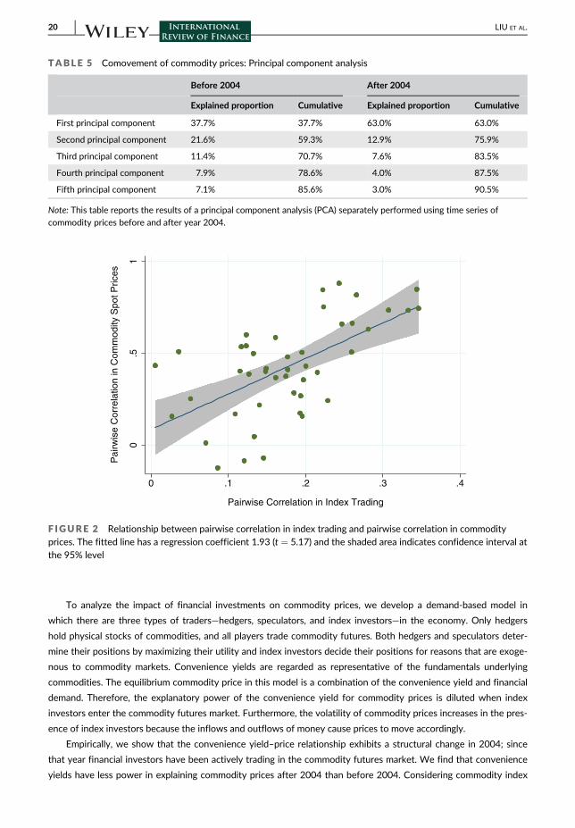
prices for fundamentally independent commodities because financial demands are correlated. Applying a principal

component analysis, we shows that the first principal component explains 37.7% and 63.0% of the variation in spot

prices before 2004 and after 2004, respectively.

In the literature, there have been heated debates about whether high commodity prices, especially during the

2007–2008 period, were caused by real demand or by financial demand. Masters and White (2008) argue that

money inflows into the commodity market have sent oil and other commodity prices beyond their fundamental

values. However, Krugman (2008) and Hamilton (2009) argue against the financial demand story, claiming that the

inflated prices of commodities were due to high worldwide demand and the inelasticity of the world supply. Their

main evidence is that if investment causes high oil prices then people would expect to see stock buildups; in contrast,

the publicly announced oil inventory data (such as the one published by the Energy Information Administration of

the USA) did not support the stockpile of inventory. From our point of view, however, it is very difficult to track

2 LIU ET AL.

commodity stocks; for example, it is impossible to count the oil stocks in Asian countries or in tankers at sea. Hence,

using inventory data would be problematic.

Traditionally, when inventory data are impossible to obtain, researchers such as Fama and French (1988) and

many others use the convenience yield5 instead because the convenience yield is the marginal value of holding one

unit of inventory and hence reflects the extent of scarcity for a certain commodity. The theory of storage (see

Brennan, 1958; Pindyck, 2001 and Telser, 1958) holds that a negative relationship exists between the convenience

yield and inventory. For example, if the high oil price in mid-2008 was due to high demand and the inelasticity of

supply, the “unobservable” inventory should be quite low, and hence the marginal value of holding one unit of inven-

tory should have been quite high, and hence, the convenience yield should also have been high. However, the conve-

nience yield did not shoot up in 2008, which indicates that holding oil inventory was inexpensive. Therefore, we

conjecture that the “unobservable” oil inventory is likely to be quite large in 2008, which makes the benefit of hold-

ing it quite low. Hence, it is likely that financial demand drove up commodity prices in the 2004–2008 period.

Thus, our paper relates to the literature on the financialization of commodities. For example, Tang and

Xiong (2012) argue that large amounts of index investment in commodity futures markets have precipitated the

financialization process with respect to commodities. Singleton (2011) estimates money inflow into the oil market

and shows that the money inflow indeed predicts price changes in the oil market. Gilbert (2009) documents that

index-based investment in commodity futures Granger-caused a significant and bubble-like increase in energy and

metal prices. Mou (2010) documents that the rolling activity of commodity index investors impacts futures prices.

Basak and Pavlova (2016) study the impact of commodity financialization on futures prices. Ekeland et al. (2017) ana-

lyze commodity financialization using both the hedging pressure theory and the storage theory. Sockin and

Xiong (2015), Goldstein et al. (2014), and Goldstein and Yang (2018) study the informativeness of asset prices by

commodity financialization. Da et al. (2020) show that index trading affects return autocorrelations among commodi-

ties in that index. Our paper distinguishes from the literature by studying the relationship between convenience

yields and commodity prices and how financial demands affect commodity prices.

Moreover, the general idea that the trading behavior of the various players in the commodity futures market

can influence prices goes back to the theory of normal backwardation, proposed by Keynes (1923) and Hicks (1939),

Hirshleifer (1988 and 1990), and Bessembinder (1992). Specifically, the theory of normal backwardation proposes

that hedgers have to sell futures prices at relatively lower prices (i.e., offer a risk premium to speculators) to solicit

speculators to come into the futures market.

For the behaviors of futures prices and convenience yields, Ng and Pirrong (1996) show a positive relationship

between convenience yields and the volatility of commodity prices, and Liu and Tang (2008) document the hetero-

skedasticity of convenience yields. Girma and Paulson (1999) investigate risk arbitrage opportunities for petroleum

futures, and Chinn and Coibion (2009) investigate the predictive components of futures prices. Our paper differs

from theirs in its focus on how the financial demand or a structural break affects the relationship between conve-

nience yields and commodity prices. For the same reason, our paper is also distinct from the literature on returns

and risk premium of commodities.6

Our paper treats financial investments as an exogenous demand shock, so it also falls into the literature on

demand-based asset pricing models that have been applied to many financial products. For example, Garleanu

et al. (2009) study demand-based option pricing in which risk-averse arbitrageurs face demand in the options market,

but take the jump risk. Greenwood and Vayanos (2010) consider the fixed-income market. In their models, the exog-

enous demand is the supply of government bonds. Greenwood (2005) and Hau (2009) consider demand shocks on

cross-sectional equity returns. In these papers, the demand shocks come from the revisions of the Nekkie or Morgan

Stanley Capital International (MSCI) index, which in turn affects the portfolio holdings of institutional investors.

The remainder of this paper is organized as follows. Section 2 documents the stylized facts for conveyance

yields and commodity prices. Section 3 presents the structural model and model predictions. Section 4 describes the

data. Section 5 tests the model empirically and Section 6 concludes.

LIU ET AL. 3

2 | CONVENIENCE YIELDS AND COMMODITY PRICES BEFORE ANDAFTER 2004

As documented by Tang and Xiong (2012), we regard 2004 as the structural break for the commodity market

because after 2004, financial investments from institutional investors rapidly flowed into the commodity futures

market. Considering the magnitude of financial investments, we conjecture that this investment flow leads to signifi-

cant changes on commodity prices. Our first observation is on the convenience yield, which is regarded as a proxy

for fundamentals and should have a stable relationship with commodity prices (e.g., Pindyck, 1993). To see whether

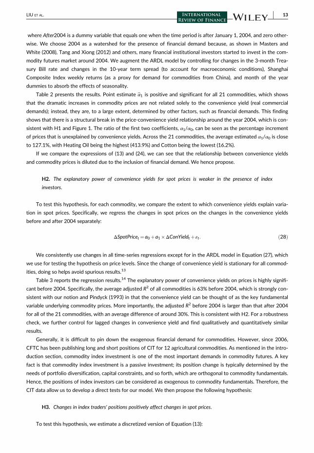
financial investments have an impact after 2004, we show some preliminary results in Figure 1.

Figure 1 plots the relationship between commodity prices and convenience yields for four major commodities.

Before 2004, convenience yields and spot prices comoved strongly, and the relationship was very stable. However,

afterward, the comovement became weaker, and the two variables sometimes even moved in opposite directions. It

is clear that the structural break has significant effects on commodities, and convenience yield does not appear to be

the main driver for commodity prices. Since the structural break is due to financial investments, we conjecture that

the demand shock from institutional investors is the reason for the dilution of the relationship. To examine our con-

jecture, in what follows, we analyze the effect of financial investment within a demand-based framework and empiri-

cally test the model predictions.

3 | A DEMAND-BASED MODEL

We regard financial investments as a demand shock and therefore adopt a demand-based framework for our analy-

sis. The model setup is as follows.

05

00

10

00

15

00

20

00

1990 1995 2000 2005 2010 2015 2020

Spot Price Convenience Yield

Soybeans

-50

05

01

00

15

0

1990 1995 2000 2005 2010 2015 2020

Spot Price Convenience Yield

Crude Oil

0100

200

300

400

500

1990 1995 2000 2005 2010 2015 2020

Spot Price Convenience Yield

Copper

-50

05

0100

150

200

1990 1995 2000 2005 2010 2015 2020

Spot Price Convenience Yield

Live Cattle

F IGURE 1 Prices and convenience yields of four commodities: Soybean, crude oil, copper, and live cattle, from

January 1990 to December 2019

4 LIU ET AL.

3.1 | Model setup

In the economy, there are three types of assets: a physical commodity, its associated commodity futures, and a risk-

free money market account. A physical commodity with spot price St pays out benefits in the form of the conve-

nience yield to its holder.7 The cumulative convenience yield Dt is governed by the process

dDt ¼ δtdt ð1Þ

and

dδt ¼ b� lδtð Þdtþσ1dB1,t, ð2Þ

where δ is the rate of the convenience yield and B denotes a Brownian motion. The convenience yield, summary of

economic status, is assumed to be exogenous in the model as the determinants of the convenience yields are not

focal points of this paper. Notably, although the convenience yield can be modeled endogenously,8 the exogenously

specified convenience yield bypasses the difficulty of modeling the consumption and production of commodities.

This assumption is also consistent with existing studies such as Gibson and Schwartz (1990) and Pindyck (1993).

Following Breeden (1984) and Ho (1984), we assume a futures contract of instantaneous maturity (denoted as

Ft≔ limT!t

F t,Tð Þ) on spot price St as an asset with a payoff in the next instant that is equal to the spot price. When an

instantaneous-maturity futures contract is assumed to exist at all times for a certain commodity, the implication is

that at every instant a futures contract expires, and another one is created in the meantime. Note that we use instan-

taneous futures contracts in this paper mainly for the sake of parsimony.9 From the cost of the carry relationship,

futures with instantaneous maturity, Ft, follow

Ft ¼ limT!t

F t,Tð Þ¼ limT!t

Ster T�tð Þ �

ðT

tdDt

� �ð3Þ

Except for physical commodities and their associated futures, investors have access to a risk-free money-market

account that pays out constant interest rates r > 0.

There are three types of agents in the economy: hedgers, speculators (or arbitrageurs), and index inves-

tors. Agents of the first type are hedgers, who are equipped with commodity containers and thus can hold

physical commodities. There are many homogeneous hedgers in the model, with mass normalized to one. We

assume that each hedger possesses inventory of a constant a unit of a physical commodity. In addition, she

can write futures hedging on her physical commodity and invest in a money market account to achieve better

lifetime utility. The second agent type is the speculator, who enters the commodity futures market as an arbi-

trageur who tends to arbitrage away any mispricing caused by hedgers and index investors and in the mean-

time allows the market to clear. The number of homogeneous speculators is w. Note that speculators only buy

or sell “paper-based” futures contracts, since they do not have physical containers to hold physical commodi-

ties. Speculators maximize their utility by rebalancing their wealth using commodity futures and a money mar-

ket account. Note that both hedgers and speculators know the status of the economy (i.e., the process of the

convenience yields) and make their trading decisions based on this knowledge. Agents of the third type are

homogeneous index investors with mass v, who take “paper-based” futures as a financial asset for investment.

Index investors make their trading decisions typically based on financial reasons such as portfolio diversifica-

tion needs and capital constraints, but not on fundamental real demand factors (i.e., convenience yields) in

commodity markets. We assume that each index investor's trading position et is exogenous and follows an

Ornstein–Uhlenbeck (OU) process,

LIU ET AL. 5

det ¼�ketdtþσ2dB2,t, ð4Þ

dB1,tdB2,t ¼0, ð5Þ

where k and σ2 are constants, and the correlation between the increment of financial demand and the convenience

yield is assumed to be zero because, as mentioned above, financial demand is exogenous to the commodity

market.10

For hedgers and speculators, we use subscript i = 1 for a representative hedger and i = 2 for a representative

speculator. Moreover, we assume that all agents maximize the mean–variance utility

maxϕi,tEt dWi,tð Þ� τ

2Vart dWi,tð Þ

h ii¼1,2, ð6Þ

where τ denotes the risk aversion parameter for both hedgers and speculators, and ϕi,t denotes the position in

futures contracts held by the ith i¼1,2ð Þ agent.The optimization problem is subject to the wealth processes of agents. The hedger's wealth follows

dW1,t ¼ r W1,t�aStð Þdtþa dStþdDtð Þþϕ1,tdFt ð7Þ

and the speculator's wealth follows

dW2,t ¼ rW2,tdtþϕ2,tdFt: ð8Þ

The market-clear condition is

ϕ1,tþwϕ2,tþvet ¼0, ð9Þ

which comes from the fact that the net supply of commodity futures is zero in the economy.

3.2 | Solution of equilibrium

In this section, we find an equilibrium where both hedgers and speculators maximize their utility, and the futures

market clears. Appendix A shows that the process for futures prices with instantaneous maturity follows

dFt ¼ dSt� rStdtþdDt: ð10Þ

Hence, (7) and (8) are changed to

dW1,t ¼ r W1,t�aStð Þdtþa dStþdDtð Þþϕ1,t dSt� rStdtþdDtð Þ ð11Þ

and

dW2,t ¼ rW2,tdtþϕ2,t dSt� rStdtþdDtð Þ: ð12Þ

The following proposition shows the solution of the equilibrium.

6 LIU ET AL.

Proposition 1. In equilibrium, the spot price St follows

St ¼ λ0þλ1δtþ λ2et, ð13Þ

where λ0, λ1, and λ2 are all constants, as shown in Appendix A. The optimal demands for agents 1 and 2 are

ϕ1,t ¼λ1b�λ2 kþ rð Þet� rλ0

τ λ21σ21þλ22σ

22

� � �a, ð14Þ

and

ϕ2,t ¼λ1b�λ2 kþ rð Þet� rλ0

τ λ21σ21þλ22σ

22

� � : ð15Þ

Proof. Refer to Appendix A. □.

When solving for the equilibrium, we first conjecture that the price has the form of (13) and solve the optimal

demands (14) and (15), taking λ0, λ1, and λ2 as given. Then by the market-clearing condition, we solve λ0, λ1, and λ2. It

can be shown that λ0 is a positive constant, and that λ1 is a function of λ0 and λ2. We further show that, in

Appendix A, λ2 is determined by a quadratic function.11 The quadratic function can have two positive roots; there-

fore, there are multiple equilibria.

Although there are multiple solutions to our equilibrium, we can still obtain some useful information by looking

at the properties of the equilibria. First, although there exist two solutions of λ2, both are positive. From the expres-

sions of (13), (14), and (15), it is easy for us to obtain the following properties:

1Þ ∂St∂et

≥0 ð16Þ

2Þ ∂ϕi,t

∂et≤0 i¼1,2ð Þ: ð17Þ

The first property reflects that, others equal, when financial demand increases, the commodity spot price cannot

decrease. For the second property, when the buying pressure of index investors is growing, as shown in proposi-

tion 3, the risk premium of buying futures tends to decrease. Therefore, both the hedgers and speculators should

buy less (or short more) futures. These properties are useful for our empirical analysis.

In our paper, we assume that index investors trade commodity futures for reasons of diversification. For this rea-

son, exogenous financial demand et is on the demand side. This is why we have market-clearing condition (9).

Although this is true in most cases, some financial investors may trade commodity futures for other reasons, and et is

not necessarily on the demand side. If it is on the supply side for some reason, the market-clearing condition

becomes

ϕ1,tþwϕ2,t ¼ vet ð18Þ

With this new market-clearing condition, the solutions of λ2 are negative.12 Thus, it is possible to have some

opposite results in our original model if financial investors do not trade for the reasons of diversification.

LIU ET AL. 7

What happens if there is no financial demand? The following proposition shows the result.

Proposition 2. If and only if v = 0, λ2 = 0.

Proof. Refer to (A21) in Appendix A. □.

Thus, financial demand has no effect if and only if there is no index investor. Equation (16) and Proposition 2

indicate that since λ2 is normally nonzero, financial demand does influence commodity prices. In other words, invest-

ments in commodity markets can cause commodity prices to deviate significantly from their fundamentals. Note that

our model is a partial equilibrium in that we do not model the source of financial demand directly. Intuitively, index

investors are likely to buy commodity futures for the sake of portfolio diversification. In this case, they would

achieve their goal of reducing portfolio risks in exchange for purchasing commodity futures at a relatively higher

price (than the value determined by the fundamentals of commodities).

3.3 | Comparative statics and predictions of the model

For comparative statics, we mainly study the influence of the number of index investors and speculators on com-

modity prices and the influence of the amount of physical inventory held by hedgers on commodity prices. Because

λ2 is a positive constant, (16) informs us that, as financial demand for futures grows in strength, commodity prices

tend to increase. Thus, the model shows that, due to financial demand, commodity prices can rise considerably

higher than their fundamental values.

We can find how λ0, λ1 and λ2 change in response to the amount of physical inventory held by hedgers

a from their expressions in Appendix A. λ0 decreases in the amount of inventory, because the more inventory

hedgers hold the more futures they need to short sell, and thus the greater they drag down commodity prices.

This is consistent with the theory of normal backwardation proposed by Keynes (1923). Furthermore, since λ2

measures the sensitivity of the price change on financial demand et, and the amount of physical inventory is

independent of financial demand in the model, we thus see that λ2 does not change with the amount of

inventory.

From this analysis, we infer that financial demand is key to determining commodity price deviations from funda-

mentals. As shown in Table 1, Panel B, the long position of commodity index investors (only one type of index inves-

tors) accounts for ~30% of 12 agricultural commodities on average; thus, financial demand is an important force in

determining commodity prices.

Proposition 3. The risk premium of futures Λ is

Λ¼ λ1b� rλ0�λ2 kþ rð Þet ð19Þ

Proof. From (10) we derive the physical measure

Et dFt½ � ¼ λ1b� rλ0� λ2 kþ rð Þet½ �dt

Since futures should have zero drift under the risk-neutral measure, the drift of the futures in the

physical measure is the risk premium of futures. □.

8 LIU ET AL.

TABLE 1 Summary statistics

Panel A: Summary statistics of 21 commodity futures

Commodity Start date Price unit ExchangeSpotprice mean

SpotPrice std

Con. yieldmean

Con.yield std

Num.of obs.

Chicago wheat 02/01/1990 Cents/bushel CME 449.4 170.7 �22.7 56.5 1379

Kansas wheat 02/01/1990 Cents/bushel KCBT 486.4 181.9 �15.4 52.2 1303

Corn 02/01/1990 Cents/bushel CME 335.5 145.8 �7.8 43.6 1473

Oats 27/11/1990 Cents/bushel CME 209.9 90.3 �1.8 38.7 1422

Soybeans 02/01/1990 Cents/bushel CME 821.7 310.0 30.3 84.8 1451

Soybean oil 02/01/1990 Cents/pound CME 29.6 11.3 �0.1 1.7 1470

Soybean meal 02/01/1990 Dollars/ton CME 253.7 95.7 17.4 33.5 1309

Crude oil 02/01/1990 Dollars/barrel NYMEX 47.2 29.7 0.9 5.2 1487

Heating oil 02/01/1990 Cents /gallon NYMEX 137.3 89.9 1.5 11.3 1432

Natural gas 27/01/1992 Dollar/MMBtu NYMEX 4.0 4.2 �0.2 2.1 1474

Cotton 02/01/1990 Cents/pound ICE 69.1 22.4 1.7 12.1 1524

Orange juice 02/01/1990 Cents/pound ICE 118.0 35.9 �2.2 11.5 1436

Cocoa 02/01/1990 Dollars/ton ICE 1845.0 748.0 �28.8 76.6 1534

Sugar 02/01/1990 Cents/pound ICE 12.8 5.6 0.4 1.7 1528

Coffee 02/01/1990 Cents/pound ICE 118.6 47.7 �4.5 15.4 1542

Platinum 02/01/1990 Dollars/troyounce

NYMEX 855.4 467.8 16.3 44.5 1487

Palladium 02/01/1990 Dollars/troyounce

NYMEX 366.4 241.6 6.2 21.3 1371

Copper 02/01/1990 Cents/pound NYMEX 180.8 111.0 7.1 13.1 1342

Lean hogs 02/01/1990 Cents/pound CME 64.3 17.5 1.0 13.9 1389

Live cattle 02/01/1990 Cents/pound CME 90.7 25.5 2.4 9.9 1486

Feeder cattle 30/01/1990 Cents/pound CME 108.0 37.9 3.5 8.9 1448

Panel B: Summary statistics of 12 agricultural commodity futures (sample mean)

Commodities Long Short Long/OI (%) Short/OI (%) Num. of obs.

Chicago Wheat 188.3 29.3 36.4 5.5 658

Kansas Wheat 46.1 6.0 24.7 2.5 713

Corn 422.2 63.3 24.0 3.4 657

Soybeans 166.6 26.8 22.3 3.2 657

Soybean oil 95.1 10.9 25.0 2.7 656

Cotton 77.5 6.9 28.9 2.4 714

Cocoa 33.6 8.1 15.4 3.1 716

Sugar 271.6 45.8 28.0 4.6 716

Coffee 48.7 6.8 23.1 2.6 716

Lean hogs 86.3 6.1 33.9 2.1 653

Live cattle 112.2 3.9 31.5 1.0 658

Feeder cattle 9.0 0.9 21.0 2.0 655

Note: Panel A of this table summarizes the characteristics of the 21 commodity futures from January 1990 to December2019 in a weekly frequency. Spot prices are calculated with futures prices following Pindyck (2001), and convenience yieldsare annualized. Panel B reports the average long and short positions of the commodity index traders for the 12 agriculturalcommodities. The sample period covers from January 2006 to December 2019 in a weekly frequency. Long/OI and short/OI are index traders' long and short positions as fractions of total open interests.

LIU ET AL. 9

As shown before, more physical inventory held by hedgers increases the selling (hedging) pressure on futures

and in turn causes a smaller λ0, thus increasing the risk premium of commodity futures. This is also consistent with

the theory of normal backwardation. In this theory, hedgers provide speculators with risk premiums to entice them

to enter the market; the stronger the hedging pressure is, the higher the risk premiums. More importantly, (19) shows

that the risk premium also depends on financial demand et, a more financial demand corresponds to a lower risk pre-

mium. This is because the financial demand offsets the hedging pressure of the hedgers and thus lowers the risk

premium. Therefore, as shown in Brunetti and Reiffen (2010), the existence of index investors makes it easier for

hedgers to hedge their physical positions.

Proposition 4. The volatility of spot price σS is

σS ¼ffiffiffiffiffiffiffiffiffiffiffiffiffiffiffiffiffiffiffiffiffiffiffiffiλ21σ

21þλ22σ

22

qð20Þ

Proof. From (13).

dSt ¼ λ1 b� lδtð Þ�λ2ket½ �dtþλ1σ1dB1,tþλ2σ2dB2,t

¼ λ1 b� lδtð Þ�λ2ket½ �dtþffiffiffiffiffiffiffiffiffiffiffiffiffiffiffiffiffiffiffiffiffiffiffiffiλ21σ

21þλ22σ

22

qdB3,t,

where B3,t is a Brownian motion. □.

This proposition indicates that the uncertainty of financial demand impacts the volatility of the commodity spot

price. λ1σ1 is the volatility of prices without index investors, andffiffiffiffiffiffiffiffiffiffiffiffiffiffiffiffiffiffiffiffiffiffiffiffiλ21σ

21þλ22σ

22

qis the volatility with index investors;

hence, the presence of index investors increases the volatility of commodity spot prices.

Proposition 5. As an extension of the model, for an economy with multiple commodities, even though dif-

ferent commodities may have independent real demands, their prices can be correlated when both are sub-

ject to correlated financial demand.

Proof. The spot prices of two commodities are

dS1t ¼ λ11 b1� l1δ1t

� �� λ12k

1e1t

h idtþλ11σ

11dB

11,tþλ12σ

12dB

12,t

dS2t ¼ λ21 b2� l2δ2t

� �� λ22k

2e2t

h idtþλ21σ

21dB

21,tþλ22σ

22dB

22,t

where superscripts of the variables identify the commodity. It is easy to show that, even though there is no correla-

tion between the fundamentals of dB11,t and dB2

1,t, if there is a correlation between the increments of financial

demand dB12,t and dB2

2,t, then the correlation between dS1t and dS2t can still be fairly large. □.

As financial demand is typically influenced by common macroeconomic factors and investors' risk appetite,

financial demand for different commodities is likely to be correlated. Moreover, as many index investors invest in

commodity indexes (i.e., buy or sell different commodities simultaneously), financial demand among different com-

modities is likely to be correlated. This is consistent with Tang and Xiong (2012), who show that the correlation

between fundamental-uncorrelated commodities such as oil and copper rose dramatically after 2004 because of

financial demands. Hence, financial demand for different commodities can be considered as a driving source of the

high correlations among different commodities observed in recent years.

10 LIU ET AL.

4 | DATA

Our data set consists of futures contracts for 21 US traded commodities, which can be classified into five groups. The

grain group includes Chicago wheat, Kansas wheat, corn, oat, soybeans, soybean oil, and soybean meal; the energy

group includes crude oil, heating oil, and natural gas; the soft group includes cotton, orange juice, cocoa, sugar, and cof-

fee; the metal group includes platinum, palladium, and copper; and the live cattle group includes lean hogs, live cattle,

and feeder cattle. Note that we do not include gold or silver in our sample since neither normally has a “real” usage and

hence does not have a significant convenience yield. For all commodity futures, we use weekly data from January 1990

to December 2019. Commodity futures prices are obtained from the Deep History Package of the Individual Commod-

ity Contracts Database of Pinnacle Data Corporation. For each weekly observation, we assign a near-month contract

and a far-month contract when computing spot prices and convenience yields. To adjust the seasonality in many com-

modity futures (e.g., Richter & Sorensen, 2002), we generally used future contracts with a time to maturity of ~1 month

and 13 months, except for several commodity futures whose 13-month futures price data are not available, for which

use futures contracts with shorter time to maturity as far-month contracts instead.

We obtain historical weekly long and short positions of commodity index traders (CIT) from the CIT report from

the commodity futures trading commission (CFTC, 2008), where futures traders are divided into three classes: com-

mercial traders, index traders, and noncommercial traders. The CIT report shows historical long and short positions

for 12 commodities: corn, soybean, Chicago wheat, Kansas wheat, soybean oil, coffee, cotton, sugar and cocoa,

feeder cattle, lean hogs, and live cattle. The major commodity indexes are Standard & Poor's–Goldman Sachs Com-

modity Index (S&P-GSCI) and the Dow Jones-UBS Commodity Index (DJ-UBSCI) and nearly all are based on passive,

long-only, fully collateralized commodity futures positions. The interest rate is based on data on 3-month Constant

Maturity Treasury (CMT) yield from the Federal Reserve Board. Table 1 shows the summary statistics for the 21 com-

modities and index trader positions on 12 agricultural commodities. One can see that CIT mainly take long positions

in commodity futures, as the average net long (long-minus-short) position is ~25% of the total open interest.

5 | HYPOTHESES AND EMPIRICAL EVIDENCE

Spot prices of commodities are usually not available, and one can use the prices of futures contracts for delivery in

the current month (spot futures contract) as the proxies. However, even spot futures contracts are not available for

every month. For this reason, we follow Pindyck (2001) and use the Equation (21) to infer the spot prices of com-

modities by extrapolating the traded futures prices:

St ¼ F t,T1ð Þ F t,T1ð ÞF t,T2ð Þ

� � T1�tT2�T1 ð21Þ

where F(t, T1) and F(t, T2) are prices of the near-month and far-month futures contracts with maturity T1 and T2

(T1 < T2). We then extract the annualized convenience yield from spot and futures prices by discretizing (3),

δt ¼ Stþ rStT2�F t,T2ð ÞT2

ð22Þ

¼ St�F t,T2ð ÞT2

þ rSt ð23Þ

where r is the 3-month CMT interest rate. Note that the measure of convenience yield includes both the commodity's con-

venience yield and its storage cost. Because the data of storage costs for various commodities are usually unavailable, we

LIU ET AL. 11

use the combination as a proxy for real convenience yields. Thus, although the extracted convenience yield measure

includes the commodity's storage cost, for expositional simplicity we refer to it as convenience yield throughout the paper.

Pindyck (1993) shows that, by analogy to the stock market (refer to Campbell & Shiller, 1987), for commodities,

the present value model of commodities is written as,

St ¼ λ0þ λ1δt: ð24Þ

This is exactly the case when no financial demand (when λ2 = 0 in Equation (13)) exists in our model. Given the same

convenience yields, financial demands have two effects on commodity prices when comparing (13) and (24). First, as shown

in the comparative statics in Section 3.2, λ0 become larger with index investors coming into the market. Second, financial

demand itself influences the price through the channel of λ2et in Equation (13). Hence, we propose the following hypothesis:

H1. Holding convenience yields the same, commodity prices rise when index investors buy commodity

futures.

To test this hypothesis, we estimate the relationship between the level of commodity prices and financial invest-

ment. Before running the time-series test, we first check the order of integration of both spot prices and conve-

nience yields. Using augmented Dickey-Fuller tests, we find that most commodity prices are I 1ð Þ, while the

convenience yields are I 0ð Þ. Since some of the variables are non-stationary, it is necessary to apply a cointegration

analysis to allow for a long-term relationship between commodity prices and convenience yields. However, the stan-

dard cointegration techniques, for example, Engle and Granger (1987) and Johansen (1991), require that all variables

be integrated in the same order and thus are not applicable in this paper. Pesaran and Shin (1999) show that an auto-

regressive distributed lag (ARDL) model can be used in the presence of a long-run relationship between the underly-

ing variables and to provide a consistent estimator of long-run parameters in the presence of the I 0ð Þ and I 1ð Þvariables in the estimation. The ARDL model is written as:

yt ¼ h0ztþXpi¼1

hyi yt�iþXqi¼0

hxi xt�iþεt ð25Þ

where y is the dependent variable, x are the regressors, z stands for the deterministic variables such as time trends

and dummy variables, and εt is a noise variable. The long-run relationship between z, x and y, yt = αzzt + αxxt, can be

calculated with αz ¼ h0

1�Ppi¼1

hyi

and αx ¼Pqi¼0

hxi

1�Ppi¼1

hyi

. Pesaran and Shin (1999) also show that the ARDL estimators are numer-

ically identical to the OLS estimators of Bewley (1979):

yt ¼ αzztþαxxtþXp�1

i¼0

βiΔyt�iþXq�1

i¼0

γiΔxt�i: ð26Þ

To estimate the statistical inference of the long-term parameters, we employ the Bewley (1979) methodology.

In our case, we choose p = 3 and q = 3 and estimate the following regression for each commodity:

SpotPricet ¼ α0þα1After2004þα2ConYieldtþX2i¼0

βiΔSpotPricet�i

þX2i¼0

γiΔConYieldt�iþΓ0Controlstþϵt

ð27Þ

12 LIU ET AL.

where After2004 is a dummy variable that equals one when the time period is after January 1, 2004, and zero other-

wise. We choose 2004 as a watershed for the presence of financial demand because, as shown in Masters and

White (2008), Tang and Xiong (2012) and others, many financial institutional investors started to invest in the com-

modity futures market around 2004. We augment the ARDL model by controlling for changes in the 3-month Trea-

sury Bill rate and changes in the 10-year term spread (to account for macroeconomic conditions), Shanghai

Composite Index weekly returns (as a proxy for demand for commodities from China), and month of the year

dummies to absorb the effects of seasonality.

Table 2 presents the results. Point estimate bα1 is positive and significant for all 21 commodities, which shows

that the dramatic increases in commodity prices are not related solely to the convenience yield (real commercial

demands); instead, they are, to a large extent, determined by other factors, such as financial demands. This finding

shows that there is a structural break in the price-convenience yield relationship around the year 2004, which is con-

sistent with H1 and Figure 1. The ratio of the first two coefficients, α1/α0, can be seen as the percentage increment

of prices that is unexplained by convenience yields. Across the 21 commodities, the average estimated α1/α0 is close

to 127.1%, with Heating Oil being the highest (413.9%) and Cotton being the lowest (16.2%).

If we compare the expressions of (13) and (24), we can see that the relationship between convenience yields

and commodity prices is diluted due to the inclusion of financial demand. We hence propose.

H2. The explanatory power of convenience yields for spot prices is weaker in the presence of index

investors.

To test this hypothesis, for each commodity, we compare the extent to which convenience yields explain varia-

tion in spot prices. Specifically, we regress the changes in spot prices on the changes in the convenience yields

before and after 2004 separately:

ΔSpotPricet ¼ a0þa1�ΔConYieldtþ εt: ð28Þ

We consistently use changes in all time-series regressions except for in the ARDL model in Equation (27), which

we use for testing the hypothesis on price levels. Since the change of convenience yield is stationary for all commod-

ities, doing so helps avoid spurious results.13

Table 3 reports the regression results.14 The explanatory power of convenience yields on prices is highly signifi-

cant before 2004. Specifically, the average adjusted R2 of all commodities is 63% before 2004, which is strongly con-

sistent with our notion and Pindyck (1993) in that the convenience yield can be thought of as the key fundamental

variable underlying commodity prices. More importantly, the adjusted R2 before 2004 is larger than that after 2004

for all of the 21 commodities, with an average difference of around 30%. This is consistent with H2. For a robustness

check, we further control for lagged changes in convenience yield and find qualitatively and quantitatively similar

results.

Generally, it is difficult to pin down the exogenous financial demand for commodities. However, since 2006,

CFTC has been publishing long and short positions of CIT for 12 agricultural commodities. As mentioned in the intro-

duction section, commodity index investment is one of the most important demands in commodity futures. A key

fact is that commodity index investment is a passive investment; its position change is typically determined by the

needs of portfolio diversification, capital constraints, and so forth, which are orthogonal to commodity fundamentals.

Hence, the positions of index investors can be considered as exogenous to commodity fundamentals. Therefore, the

CIT data allow us to develop a direct tests for our model. We then propose the following hypothesis:

H3. Changes in index traders' positions positively affect changes in spot prices.

To test this hypothesis, we estimate a discretized version of Equation (13):

LIU ET AL. 13

TABLE2

Commodity

prices

before

andafter2004

Commodity

Intercep

tAfter2004

CYt

ΔSP

tΔCYt

ΔSP

t�

1ΔCYt�

1ΔSP

t�

2ΔCYt�

2R2

Chicago

whe

at316.5***

280.9***

1.1***

0.5

�1.0**

0.3

�1.1**

0.4

�1.0*

0.55

(22.4)

(37.9)

(14.5)

(1.4)

(�2.1)

(1.1)

(�2.4)

(1.2)

(�1.8)

Kan

saswhe

at324.3***

292.7***

1.4***

0.3

�1.0*

0.3

�1.2**

0.4

�1.0*

0.45

(20.3)

(37.2)

(18.6)

(1.0)

(�1.7)

(0.9)

(�2.2)

(1.2)

(�1.9)

Corn

241.4***

202.3***

2.1***

0.7**

�1.6***

0.5*

�1.0***

0.4

�0.9**

0.77

(38.4)

(51.4)

(39.1)

(2.5)

(�4.1)

(1.9)

(�2.7)

(1.6)

(�2.3)

Oats

138.7***

136.1***

0.8***

0.5**

�0.7***

0.5**

�0.7***

0.4*

�0.5**

0.67

(30.1)

(46.3)

(20.4)

(2.0)

(�3.0)

(2.1)

(�3.2)

(1.7)

(�2.6)

Soyb

eans

540.1***

431.0***

1.8***

0.7**

�1.4***

0.6**

�1.2**

0.6**

�1.4**

0.73

(35.9)

(46.5)

(16.4)

(2.5)

(�2.6)

(2.1)

(�2.0)

(2.2)

(�2.4)

Soyb

eanoil

20.9***

17.7***

1.3***

0.5

�0.4

0.3

�0.3

0.4

�0.7

0.50

(25.2)

(36.6)

(14.1)

(1.3)

(�0.6)

(0.8)

(�0.3)

(1.1)

(�0.9)

Soyb

eanmea

l155.6***

119.5***

1.7***

0.8***

�1.4***

0.6***

�1.0***

0.5***

�0.8***

0.79

(31.6)

(43.6)

(31.6)

(3.5)

(�4.6)

(3.0)

(�3.7)

(2.9)

(�3.3)

Crude

oil

15.3***

58.0***

2.0***

0.4

�1.5***

0.4

�1.4***

0.4

�1.1**

0.87

(11.4)

(69.4)

(26.3)

(1.4)

(�3.0)

(1.3)

(�2.7)

(1.5)

(�2.2)

Hea

ting

oil

43.3***

179.2***

2.5***

0.2

�1.4**

0.2

�1.3**

0.3

�0.8

0.80

(10.7)

(64.5)

(22.2)

(0.7)

(�2.1)

(0.8)

(�2.0)

(1.0)

(�1.3)

Naturalgas

1.8***

3.1***

1.7***

0.5

�1.2**

0.4

�0.9*

0.4

�0.7

0.83

(7.4)

(14.4)

(6.5)

(1.4)

(�2.0)

(1.0)

(�1.7)

(1.0)

(�1.5)

Cotton

61.2***

9.9***

1.7***

0.3*

�0.7***

0.3*

�0.7***

0.3*

�0.7***

0.85

(73.0)

(21.3)

(88.6)

(1.9)

(�3.4)

(1.7)

(�3.3)

(1.8)

(�3.2)

Orang

ejuice

107.3***

37.2***

2.2***

0.6***

�1.2***

0.6***

�1.1***

0.4***

�0.9***

0.46

(57.1)

(41.8)

(51.4)

(5.3)

(�5.5)

(5.6)

(�5.5)

(4.4)

(�4.1)

Coco

a1368.2***

1058.8***

2.9***

0.4***

�1.8***

0.5***

�1.7***

0.4***

�1.6***

0.65

(28.7)

(42.0)

(18.3)

(2.7)

(�3.3)

(3.7)

(�3.2)

(3.0)

(�2.9)

14 LIU ET AL.

TABLE2

(Continue

d)

Commodity

Intercep

tAfter2004

CYt

ΔSP

tΔCYt

ΔSP

t�

1ΔCYt�

1ΔSP

t�

2ΔCYt�

2R2

Sugar

7.5***

8.4***

2.0***

0.3*

�1.0***

0.2

�0.9***

0.3

�0.8**

0.75

(25.4)

(54.3)

(51.1)

(1.7)

(�3.0)

(1.2)

(�2.8)

(1.3)

(�2.5)

Coffee

96.0***

62.7***

1.9***

0.5*

�1.4***

0.5*

�1.4***

0.4

�1.2**

0.52

(31.8)

(33.0)

(35.4)

(1.8)

(�3.3)

(1.8)

(�2.8)

(1.5)

(�2.3)

Platinu

m416.0***

826.8***

0.9***

0.4

�0.8**

0.6*

�0.3

0.5

�0.2

0.75

(16.7)

(53.0)

(3.5)

(1.2)

(�2.5)

(1.7)

(�1.4)

(1.5)

(�1.3)

Palladium

179.5***

343.9***

4.4***

0.3

�2.9***

0.4

�2.5**

0.2

�2.3**

0.52

(8.8)

(26.7)

(7.2)

(0.7)

(�2.6)

(1.2)

(�2.4)

(0.7)

(�2.4)

Copp

er94.0***

200.4***

0.1

0.3

�0.7

0.2

�0.5

0.3

�0.6

0.79

(16.1)

(59.6)

(0.5)

(0.9)

(�0.8)

(0.7)

(�0.6)

(1.1)

(�0.6)

Lean

hogs

47.5***

24.4***

0.7***

0.6***

�0.4***

0.5***

�0.4***

0.4***

�0.2**

0.63

(52.4)

(39.5)

(24.3)

(3.9)

(�3.4)

(3.9)

(�3.7)

(2.9)

(�2.0)

Live

cattle

66.7***

42.4***

0.8***

0.4

�0.2

0.4

�0.2

0.2

�0.1

0.63

(40.1)

(44.3)

(14.9)

(1.2)

(�0.8)

(1.1)

(�0.5)

(0.7)

(�0.2)

Fee

dercattle

74.8***

58.1***

0.9***

0.5

�0.4

0.3

0.1

0.4

�0.3

0.56

(28.3)

(38.0)

(8.9)

(0.9)

(�0.6)

(0.6)

(0.1)

(0.7)

(�0.5)

Note:Thistablerepo

rtsregressions

ofco

mmodity

spotprices

onco

nven

ienc

eyields

(CY),an

dch

ange

sin

both

spotprices

(ΔSP

),an

dco

nve

nience

yields(ΔCY),as

wellastheirlagg

ed

term

s,forthe21co

mmodities.T

hesampleisfrom

Janu

ary1990to

Decem

ber2019in

awee

klyfreq

uenc

y,an

dAfter2004isadummyvariab

lethat

equalsoneforobservationsafter

Janu

ary1,2

004.A

dditiona

lcontrolvariables

includ

ech

ange

sin

3-m

onthTreasurybillrate

and10-yea

r–3-m

onthTreasuryyieldspread

,Shan

ghaico

mposite

index

return,andmonth

of

theye

ardu

mmies.Su

perscripts

***,**,and

*indicate

statisticalsignificanc

eat

the1%,5

%,and

10%

leve

ls,respe

ctively.

LIU ET AL. 15

TABLE 3 Decrease in explanatory power of convenience yield on commodity prices

Before 2004 After 2004

Commodity Intercept ΔCYt R2 Intercept ΔCYt R2 Difference in R2

Chicago wheat �0.02 1.18*** 0.64 0.39 1.09*** 0.28 0.36

(�0.06) (13.52) (0.40) (7.64)

Kansas wheat �0.00 1.23*** 0.64 0.64 0.18*** 0.20 0.44

(�0.00) (13.95) (0.64) (10.07)

Corn 0.01 1.07*** 0.58 0.39 0.95*** 0.37 0.21

(0.04) (7.95) (0.62) (11.32)

Oats �0.01 0.77*** 0.63 �0.02 0.75*** 0.50 0.13

(�0.07) (18.36) (�0.04) (17.69)

Soybeans 0.04 1.04*** 0.61 1.20 0.97*** 0.39 0.22

(0.07) (23.35) (1.01) (7.99)

Soybean oil 0.00 1.20*** 0.49 0.02 0.08*** 0.03 0.46

(0.10) (25.97) (0.34) (8.20)

Soybean meal �0.00 1.00*** 0.68 0.53 1.08*** 0.64 0.04

(�0.01) (27.52) (1.42) (20.37)

Crude oil 0.03 1.31*** 0.85 0.11 1.37*** 0.33 0.52

(1.45) (35.48) (0.77) (13.59)

Heating oil 0.08 1.31*** 0.81 0.18 0.38* 0.11 0.70

(1.38) (32.59) (0.55) (1.80)

Natural gas 0.01 2.04*** 0.86 �0.01 1.13*** 0.66 0.20

(0.17) (9.94) (�0.52) (12.02)

Cotton �0.02 1.14*** 0.79 0.03 1.15*** 0.73 0.06

(�0.39) (40.89) (0.39) (21.42)

Orange juice �0.07 1.34*** 0.54 0.16 0.18*** 0.17 0.37

(�0.57) (7.71) (0.62) (6.41)

Cocoa 0.55 4.09*** 0.41 �0.84 0.11*** 0.18 0.23

(0.16) (3.50) (�0.24) (3.67)

Sugar �0.00 1.37*** 0.75 0.01 1.43*** 0.68 0.07

(�0.42) (33.58) (0.28) (18.93)

Coffee 0.05 1.11*** 0.51 0.10 1.88*** 0.21 0.30

(0.26) (7.75) (0.47) (5.89)

Platinum 0.51 0.44*** 0.54 0.40 1.29*** 0.07 0.47

(1.01) (66.76) (0.23) (3.50)

Palladium 0.12 1.65*** 0.26 0.66 �0.05 0.00 0.26

(0.14) (3.67) (0.69) (�0.20)

Copper 0.03 1.33*** 0.66 0.43 2.68*** 0.31 0.35

(0.47) (30.35) (0.88) (7.46)

Lean hogs 0.03 0.69*** 0.66 0.09 0.38*** 0.47 0.19

(0.40) (12.20) (0.86) (5.42)

Live cattle 0.03 1.05*** 0.72 0.06 0.40*** 0.35 0.37

16 LIU ET AL.

TABLE 3 (Continued)

Before 2004 After 2004

Commodity Intercept ΔCYt R2 Intercept ΔCYt R2 Difference in R2

(0.60) (16.52) (0.60) (6.41)

Feeder cattle 0.03 0.76*** 0.55 0.08 0.35*** 0.22 0.33

(0.74) (12.49) (0.67) (5.53)

Average 0.63 0.33 0.30

Note: This table reports regressions of changes in commodity prices on changes in convenience yield for 21 commodities

before and after the year of 2004. The sample is from January 1990 to December 2019 in a weekly frequency. The last

column is the difference in adjusted R2 between the two subsamples before and after the year 2004. The superscripts ***,

**, and * indicate statistical significance at the 1%, 5%, and 10% levels, respectively.

TABLE 4 Relationship between index trading positions and commodity prices

Panel A: Correlation between changes in convenience yields and changes in net long CIT positions

Commodity Correlation

Chicago Wheat 0.008

Kansas Wheat 0.027

Corn 0.056

Soybeans 0.091

Soybean Oil �0.028

Cotton 0.016

Cocoa 0.034

Sugar �0.060

Coffee 0.067

Lean Hogs 0.042

Live Cattle 0.046

Feeder Cattle �0.027

Panel B: Commodity-by-commodity regressions

Intercept ΔCYt ΔNetLongt R2

Chicago Wheat 0.37 1.08*** 0.79** 0.29

(0.36) (7.61) (2.47)

Kansas Wheat 0.37 0.18*** 3.56*** 0.24

(0.36) (11.58) (6.75)

Corn 0.42 0.94*** 0.17** 0.38

(0.61) (11.11) (2.10)

Soybeans 1.09 0.93*** 1.65*** 0.42

(0.88) (7.65) (4.51)

Soybean Oil 0.01 0.08*** 0.08*** 0.06

(0.18) (9.16) (3.73)

Cotton 0.01 1.14*** 0.09 0.73

(0.15) (21.16) (1.52)

Cocoa �1.21 0.11*** 10.33*** 0.21

(�0.34) (3.59) (4.68)

(Continues)

LIU ET AL. 17

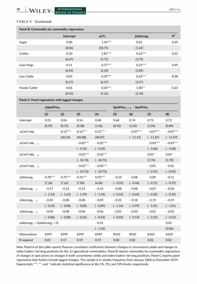
TABLE 4 (Continued)

Panel B: Commodity-by-commodity regressions

Intercept ΔCYt ΔNetLongt R2

Sugar 0.00 1.43*** 0.01 0.69

(0.06) (18.71) (1.63)

Coffee 0.10 1.81*** 0.63*** 0.23

(0.47) (5.71) (3.75)

Lean Hogs 0.11 0.37*** 0.31*** 0.49

(0.99) (5.39) (5.09)

Live Cattle 0.03 0.39*** 0.24*** 0.38

(0.27) (6.37) (3.57)

Feeder Cattle 0.06 0.34*** 1.00** 0.23

(0.45) (5.16) (2.10)

Panel C: Panel regressions with lagged changes

ΔSpotPricet SpotPricet + 3 � SpotPricet

(1) (2) (3) (4) (5) (6) (7) (8)

Intercept 0.25 0.06 0.14 0.48 0.68 0.74 0.75 0.72

(0.59) (0.15) (0.38) (1.06) (0.93) (1.02) (1.04) (0.84)

ΔConY ieldt 0.12*** 0.12*** 0.12*** �0.07*** �0.07*** �0.07***

(40.24) (40.88) (40.87) (�11.41) (�11.87) (�11.87)

ΔConY ieldt � 1 �0.02*** �0.02*** �0.03*** �0.03***

(�5.43) (�5.45) (�3.40) (�3.40)

ΔConY ieldt � 2 �0.03*** �0.03*** 0.01* 0.01*

(�10.74) (�10.73) (1.70) (1.70)

ΔConY ieldt � 3 �0.03*** �0.03*** �0.01 �0.01

(�10.72) (�10.73) (�0.95) (�0.95)

ΔNetLongt 0.78*** 0.75*** 0.76*** 0.93*** �0.10 �0.08 �0.09 �0.11

(7.26) (7.62) (7.90) (6.06) (�0.55) (�0.46) (�0.51) (�0.37)

ΔNetLongt � 1 �0.17 �0.16 �0.15 �0.15 �0.08 �0.08 �0.07 �0.06

(�1.53) (�1.62) (�1.49) (�1.54) (�0.42) (�0.43) (�0.35) (�0.35)

ΔNetLongt � 2 �0.03 �0.08 �0.08 �0.09 �0.22 �0.18 �0.19 �0.19

(�0.25) (�0.84) (�0.85) (�0.89) (�1.16) (�0.99) (�1.01) (�1.01)

ΔNetLongt � 3 �0.09 �0.08 �0.06 �0.06 �0.01 �0.03 �0.02 �0.02

(�0.86) (�0.80) (�0.63) (�0.63) (�0.03) (�0.14) (�0.12) (�0.12)

ΔNetLongt � I(ΔNetLongt > 0) �0.31 0.02

(�1.36) (0.06)

Observations 8399 8399 8399 8399 8103 8103 8103 8103

R-squared 0.01 0.17 0.19 0.19 0.00 0.02 0.02 0.02

Note: Panel A of this table reports Pearson correlation coefficients between changes in convenience yields and changes in

index traders' net long positions for the 12 agricultural commodities. Panel B reports commodity-by-commodity regressions

of changes in spot prices on changes in both convenience yields and index traders' net long positions. Panel C reports panel

regressions that further include lagged changes. The sample is in weekly frequency from January 2006 to December 2019.

Superscripts ***, **, and * indicate statistical significance at the 1%, 5%, and 10% levels, respectively.

18 LIU ET AL.

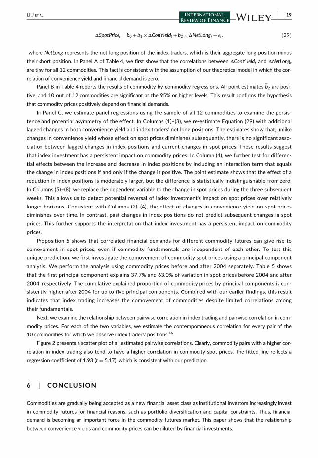
ΔSpotPricet ¼ b0þb1�ΔConYieldtþb2�ΔNetLongtþεt: ð29Þ

where NetLong represents the net long position of the index traders, which is their aggregate long position minus

their short position. In Panel A of Table 4, we first show that the correlations between ΔConY ieldt and ΔNetLongtare tiny for all 12 commodities. This fact is consistent with the assumption of our theoretical model in which the cor-

relation of convenience yield and financial demand is zero.

Panel B in Table 4 reports the results of commodity-by-commodity regressions. All point estimates bb2 are posi-

tive, and 10 out of 12 commodities are significant at the 95% or higher levels. This result confirms the hypothesis

that commodity prices positively depend on financial demands.

In Panel C, we estimate panel regressions using the sample of all 12 commodities to examine the persis-

tence and potential asymmetry of the effect. In Columns (1)–(3), we re-estimate Equation (29) with additional

lagged changes in both convenience yield and index traders' net long positions. The estimates show that, unlike

changes in convenience yield whose effect on spot prices diminishes subsequently, there is no significant asso-

ciation between lagged changes in index positions and current changes in spot prices. These results suggest

that index investment has a persistent impact on commodity prices. In Column (4), we further test for differen-

tial effects between the increase and decrease in index positions by including an interaction term that equals

the change in index positions if and only if the change is positive. The point estimate shows that the effect of a

reduction in index positions is moderately larger, but the difference is statistically indistinguishable from zero.

In Columns (5)–(8), we replace the dependent variable to the change in spot prices during the three subsequent

weeks. This allows us to detect potential reversal of index investment's impact on spot prices over relatively

longer horizons. Consistent with Columns (2)–(4), the effect of changes in convenience yield on spot prices

diminishes over time. In contrast, past changes in index positions do not predict subsequent changes in spot

prices. This further supports the interpretation that index investment has a persistent impact on commodity

prices.

Proposition 5 shows that correlated financial demands for different commodity futures can give rise to

comovement in spot prices, even if commodity fundamentals are independent of each other. To test this

unique prediction, we first investigate the comovement of commodity spot prices using a principal component

analysis. We perform the analysis using commodity prices before and after 2004 separately. Table 5 shows

that the first principal component explains 37.7% and 63.0% of variation in spot prices before 2004 and after

2004, respectively. The cumulative explained proportion of commodity prices by principal components is con-

sistently higher after 2004 for up to five principal components. Combined with our earlier findings, this result

indicates that index trading increases the comovement of commodities despite limited correlations among

their fundamentals.

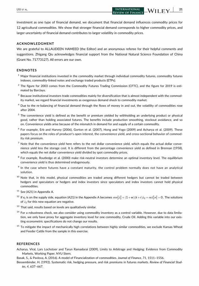
Next, we examine the relationship between pairwise correlation in index trading and pairwise correlation in com-

modity prices. For each of the two variables, we estimate the contemporaneous correlation for every pair of the

10 commodities for which we observe index traders' positions.15

Figure 2 presents a scatter plot of all estimated pairwise correlations. Clearly, commodity pairs with a higher cor-

relation in index trading also tend to have a higher correlation in commodity spot prices. The fitted line reflects a

regression coefficient of 1.93 (t = 5.17), which is consistent with our prediction.

6 | CONCLUSION

Commodities are gradually being accepted as a new financial asset class as institutional investors increasingly invest

in commodity futures for financial reasons, such as portfolio diversification and capital constraints. Thus, financial

demand is becoming an important force in the commodity futures market. This paper shows that the relationship

between convenience yields and commodity prices can be diluted by financial investments.

LIU ET AL. 19

To analyze the impact of financial investments on commodity prices, we develop a demand-based model in

which there are three types of traders—hedgers, speculators, and index investors—in the economy. Only hedgers

hold physical stocks of commodities, and all players trade commodity futures. Both hedgers and speculators deter-

mine their positions by maximizing their utility and index investors decide their positions for reasons that are exoge-

nous to commodity markets. Convenience yields are regarded as representative of the fundamentals underlying

commodities. The equilibrium commodity price in this model is a combination of the convenience yield and financial

demand. Therefore, the explanatory power of the convenience yield for commodity prices is diluted when index

investors enter the commodity futures market. Furthermore, the volatility of commodity prices increases in the pres-

ence of index investors because the inflows and outflows of money cause prices to move accordingly.

Empirically, we show that the convenience yield–price relationship exhibits a structural change in 2004; since

that year financial investors have been actively trading in the commodity futures market. We find that convenience

yields have less power in explaining commodity prices after 2004 than before 2004. Considering commodity index

TABLE 5 Comovement of commodity prices: Principal component analysis

Before 2004 After 2004

Explained proportion Cumulative Explained proportion Cumulative

First principal component 37.7% 37.7% 63.0% 63.0%

Second principal component 21.6% 59.3% 12.9% 75.9%

Third principal component 11.4% 70.7% 7.6% 83.5%

Fourth principal component 7.9% 78.6% 4.0% 87.5%

Fifth principal component 7.1% 85.6% 3.0% 90.5%

Note: This table reports the results of a principal component analysis (PCA) separately performed using time series of

commodity prices before and after year 2004.

0.5

1

Pa

irw

ise

Co

rre

latio

n in

Co

mm

od

ity S

po

t P

rice

s

0 .1 .2 .3 .4

Pairwise Correlation in Index Trading

F IGURE 2 Relationship between pairwise correlation in index trading and pairwise correlation in commodityprices. The fitted line has a regression coefficient 1.93 (t = 5.17) and the shaded area indicates confidence interval atthe 95% level

20 LIU ET AL.

investment as one type of financial demand, we document that financial demand influences commodity prices for

12 agricultural commodities. We show that stronger financial demand corresponds to higher commodity prices, and

larger uncertainty of financial demand contributes to larger volatility in commodity prices.

ACKNOWLEDGMENT

We are grateful to ALLAUDEEN HAMEED (the Editor) and an anonymous referee for their helpful comments and

suggestions. Zhigang Qiu acknowledges financial support from the National Natural Science Foundation of China

(Grant No. 71773127). All errors are our own.

ENDNOTES1 Major financial institutions invested in the commodity market through individual commodity futures, commodity futures

indexes, commodity-linked notes and exchange traded products (ETPs).2 The figure for 2003 comes from the Commodity Futures Trading Commission (CFTC), and the figure for 2019 is esti-

mated by Barclays.3 Because institutional investors trade commodities mainly for diversification that is almost independent with the commod-

ity market, we regard financial investments as exogenous demand shock to commodity market.4 Due to the re-balancing of financial demand through the flows of money in and out, the volatility of commodities rose

after 2004.5 The convenience yield is defined as the benefit or premium yielded by withholding an underlying product or physical

good, rather than holding associated futures. The benefits include production smoothing, stockout avoidance, and so

on. Convenience yields arise because of the mismatch in demand for and supply of a certain commodity.6 For example, Erb and Harvey (2006), Gorton et al. (2007), Hong and Yogo (2009) and Acharya et al. (2009). These

papers focus on the roles of producer's open interest, the convenience yield, and cross-sectional behavior of commod-

ity risk premium.7 Note that the convenience yield here refers to the net dollar convenience yield, which equals the actual dollar conve-

nience yield less the storage cost. It is different from the percentage convenience yield as defined in Brennan (1958),

which equals the net dollar convenience yield divided by spot commodity prices.8 For example, Routledge et al. (2000) make risk-neutral investors determine an optimal inventory level. The equilibrium

convenience yield is thus determined endogenously.9 In the case where futures have a constant maturity, the control problem normally does not have an analytical

solution.10 Note that, in this model, physical commodities are traded among different hedgers but cannot be traded between

hedgers and speculators or hedgers and index investors since speculators and index investors cannot hold physical

commodities.11 See (A21) in Appendix A.12 If et is on the supply side, equation (A21) in the Appendix A becomes τvσ22λ

22þ 1þwð Þ kþ rð Þλ2þ τvλ21σ

21 ¼ 0.. The solutions

of λ2 for this new equation are negative.13 That said, results based on levels are qualitatively similar.14 For a robustness check, we also consider using commodity inventory as a control variable. However, due to data limita-

tion, we only have proxy for aggregate inventory level for one commodity, Crude Oil. Adding this variable into our exis-

ting econometric specifications do not change our results.15 To mitigate the impact of mechanically high correlations between highly similar commodities, we exclude Kansas Wheat

and Feeder Cattle from the sample in this exercise.

REFERENCES

Acharya, Viral, Lars Lochstoer and Tarun Ramadorai (2009), Limits to Arbitrage and Hedging: Evidence from Commodity

Markets, Working Paper, NYU Stern.

Basak, S., & Pavlova, A. (2016). A model of Financialization of commodities. Journal of Finance, 71, 1511–1556.Bessembinder, H. (1992). Systematic risk, hedging pressure, and risk premiums in futures markets. Review of Financial Stud-

ies, 4, 637–667.

LIU ET AL. 21

Bewley, R. A. (1979). The direct estimation of the equilibrium response in a linear dynamic model. Economic Letters, 3,

357–361.Breeden, D. (1984). Futures markets and commodity options: Hedging and optimality in incomplete markets. Journal of Eco-

nomic Theory, 32, 275–300.Brennan, M. (1958). The supply of storage. American Economic Review, 48, 50–72.Brunetti, Celso and David Reiffen (2010), Commodity Index Trading and Hedging Costs, Working Paper, John Hopkins

University.

Campbell, J. Y., & Shiller, R. J. (1987). Cointegration and tests of present value models. Journal of Political Economy, 95,

1062–1088.CFTC (2008), Staff Report on Commodity Swap Dealers & Index Traders with Commission Recommendations.

Chinn, M. D., & Coibion, O. (2009). The predictive content of commodity futures. Journal of Futures Markets, 34(7),

607–636.Da, Zhi, Ke Tang, Yubo Tao and Liyan Yang (2020). Financialization and Commodity Market Serial Dependence, Working

Paper.

Ekeland, I., D. Lautier, and B. Villeneuve (2017), Hedging Pressure and Speculation in Commodity Markets, Working Paper.

Engle, R. F., & Granger, C. W. J. (1987). Co-integration and error correction: Representation, estimation, and testing. Eco-

nometrica, 55, 251–276.Erb, C., & Harvey, C. (2006). The strategic and tactical value of commodity futures. Financial Analysts Journal, 62, 69–97.Fama, E., & French, K. (1988). Business cycles and the behavior of metals prices. Journal of Finance, 43, 1075–1094.Garleanu, N., Pedersen, L., & Poteshman, A. (2009). Demand-based option pricing. Reviews of Financial Studies, 22, 4259–

4299.

Gibson, R., & Schwartz, E. (1990). Stochastic convenience yield and the pricing of oil contingent claims. Journal of Finance,

45, 959–976.Gilbert, Christopher L. (2009), Speculative Influences on Commodity Futures Prices 2006–2008, Working Paper, UNCTAD

and University of Trento.

Girma, P. B., & Paulson, A. S. (1999). Risk arbitrage opportunities in petroleum futures spreads. Journal of Futures Markets,

19(8), 931–955.Goldstein, I., Li, Y., & Yang, L. (2014). Speculation and hedging in segmented markets. Review of Financial Studies, 27,

881–822.Goldstein, I. and L. Yang (2018), Commodity Financialization and Information Transmission, Working Paper.

Gorton, Gary, Fumio Hayashi and Geert Rouwenhorst (2007), The Fundamentals of Commodity Futures Returns, Working

Paper, Yale University.

Greenwood, R. (2005). Short- and long-term demand curves for stocks: Theory and evidence on the dynamics of arbitrage.

Journal of Financial Economics, 75, 607–649.Greenwood Robin, Vayanos D. (2010), Bond supply and excess bond returns, Working Paper, Harvard University.

Hamilton, James D (2009), Causes and Consequences of the Oil Shock of 2007–2008. Working paper, UC San Diego.

Hau H. (2009), Global versus local asset pricing: evidence from arbitrage of the MSCI index change. Working Paper,

INSEAD.

Hicks, J. R. (1939). Value and capital: An inquiry into some fundamental principles of economic theory. Claredon Press.

Hirshleifer, D. (1988). Residual risk, trading costs and commodity futures risk Premia. Review of Financial Studies, 1,

173–193.Hirshleifer, D. (1990). Hedging pressure and futures price movements in a general equilibrium model. Econometrica, 58,

411–428.Ho, T. (1984). Intertemporal commodity futures hedging and the production decision. Journal of Finance, 39, 351–377.Hong, H., & Yogo, M. (2009). Digging into commodities, working paper. Princeton University and University of.

Johansen, S. (1991). Estimation and hypothesis testing of Cointegration vectors in Gaussian vector autoregressive models.

Econometrica, 59, 1551–1580.Keynes, John M. (1923), Some Aspects of Commodity Markets, Manchester Guardian Commercial: European Reconstruc-

tion Series.

Krugman, Paul (2008), The Oil Nonbubble, The New York Times, May 12.

Liu, P., & Tang, K. (2008). The stochastic behavior of commodity prices with Heteroskedasticity in the convenience yield.

Journal of Empirical Finance, 18(2), 211–224.Masters, Michael and Allen K. White (2008), The Accidental Hunt Brothers: How Institutional Investors are Driving up Food

and Energy Prices, White Paper.

Mou, Yiqun (2010), Limits to Arbitrage and Commodity Index Investments: Front-running the Goldman Roll. Technical

Report, Columbia Business School.

22 LIU ET AL.

Ng, V. K., & Pirrong, S. C. (1996). Price dynamics in refined petroleum spot and futures markets. Journal of Empirical Finance,

2(4), 359–388.Pesaran, M. H., & Shin, Y. (1999). An autoregressive distributed lag modelling approach to Cointegration analysis. In S. Strom

(Ed.), Econometrics and economic theory in the twentieth century. Cambridge University Press.

Pindyck, R. (1993). The present value model of rational commodity pricing. Economic Journal, 103, 511–530.Pindyck, R. (2001). The dynamics of commodity spot and futures markets: A primer. The Energy Journal, 22, 1–29.Richter, M. and C. Sorensen (2002): Stochastic volatility and seasonality in commodity futures and options: The case of soy-

beans, Working paper, Copenhagen Business School.

Routledge, B. R., Seppi, D. J., & Spatt, C. S. (2000). Equilibrium forward curves for commodities. Journal of Finance, 55(3),

1297–1338.Singleton, Kenneth J. (2011), Investor Flows and the 2008 Boom/Bust in Oil Prices, Working paper, Stanford University.

Sockin, M., & Xiong, W. (2015). Informational frictions and commodity markets. Journal of Finance, 70, 2063–2098.Tang, K., & Xiong, W. (2012). Index investment and the Financialization of commodities. Financial Analysts Journal, 68,

54–74.Telser, L. (1958). Futures trading and the storage of cotton and wheat. Journal of Political Economy, 66, 233–255.

How to cite this article: Liu, P., Qiu, Z., & Xu, D. X. (2021). Financial investments and commodity prices.

International Review of Finance, 1–25. https://doi.org/10.1111/irfi.12361

Appendix A: MODEL

Futures process with instantaneous maturity

We assume the futures price with instantaneous maturity follows

limT!t

F t,Tð Þ¼ Ster T�tð Þ �

ðT

tdDs ðA1Þ

Using Ito's lemma on F(t, T), we have

dF t,Tð Þ¼ er T�tð ÞdSt� rSter T�tð ÞdtþdDs ðA2Þ

Defining Δ: = T � t, if T! t, that is, Δ!0, then

dFt ≔ limT!t

dF t,Tð Þ ðA3Þ

¼ 1þ rΔð ÞdSt� rSt 1þ rΔð ÞdtþdDt ðA4Þ

¼ dSt� rStdtþdDt ðA5Þ

Solution of the equilibrium

In the equilibrium, we conjecture that the spot price St follow

St ¼ λ0þλ1δtþ λ2et, ðA6Þ

LIU ET AL. 23

For three constants λ0, λ1, and λ2. Then the spot price dSt can be specified as

dSt ¼ λ1dδtþ λ2det ðA7Þ

¼ λ1b�λ1lδt�λ2ketð Þdtþλ1σ1dB1,tþλ2σ2dB2,t ðA8Þ

Thus, the wealth processes for both hedgers and speculators, (7) and (8), are

dW1,t ¼ rW1,tþ ϕ1,tþa� �

λ1b� λ1 lþ rλ1�1ð Þδt�λ2 kþ rð Þet� rλ0ð Þ dt ðA9Þ

þ ϕ1,tþa� �

λ1σ1dB1,tþλ2σ2dB2,tð Þ ðA10Þ

dW2,t ¼ rdW2,tþϕ2,t λ1b� λ1lþ rλ1�1ð Þδt� λ2 kþ rð Þet� rλ0ð Þ dt ðA11Þ

þϕ2,t λ1σ1dB1,tþλ2σ2dB2,tð Þ ðA12Þ

By the FOC with respect to the utility, (6), we can derive the optimal demands

ϕ1,t ¼λ1b� λ1lþ rλ1�1ð Þδt�λ2 kþ rð Þet� rλ0

τ λ21σ21þ λ22σ

22

� � �a ðA13Þ

and

ϕ2,t ¼λ1b� λ1lþ rλ1�1ð Þδt�λ2 kþ rð Þet� rλ0

τ λ21σ21þ λ22σ

22

� � ðA14Þ

Together with the expression of λ1, (A19), we can obtain (14) and (15) in the proposition.

With the optimal demands (A13) and (A14), the future market-clearing condition (9) can be arranged as

1þwð Þ λ1b� rλ0ð Þ� τ λ21σ21þλ22σ

22

� �a�

1þwð Þ λ1lþ rλ1�1ð Þδtþ τ λ21σ21þ λ22σ

22

� �v� 1þwð Þλ2 kþ rð Þ

et

( )¼0 ðA15Þ

which is an affine function of δt and et. Thus, the constant and the coefficients of δt and et need to be zero.

First, the coefficient of δt needs to be zero, which means

1þwð Þ λ1lþ rλ1�1ð Þ¼0 ðA16Þ

We can derive λ1 as

λ1 ¼ 1rþ l

ðA17Þ

Second, the constant needs to be zero, which means

1þwð Þ λ1b� rλ0ð Þ� τ λ21σ21þλ22σ

22

� �a¼0 ðA18Þ

24 LIU ET AL.

We can derive λ0 as

λ0 ¼1þwð Þλ1b� τ λ21σ

21þλ22σ

22

� �a

1þwð Þr ðA19Þ

Third, the coefficient of et needs to be zero, which means

τ λ21σ21þλ22σ

22

� �v� 1þwð Þλ2 kþ rð Þ¼0 ðA20Þ

which can be rearranged as

τvσ22λ22� 1þwð Þ kþ rð Þλ2þ τvλ21σ

21 ¼0 ðA21Þ

Thus, λ2 is determined by a quadratic function (A21). Define F λ2ð Þ¼ τvσ22λ22� 1þwð Þ kþ rð Þλ2þ τvλ21σ

21, so the equi-

librium exists iff F λ2ð Þ¼0 has a positive root. Note that F 0ð Þ>0 and the solution to F0 λ2ð Þ¼0 is positive, any solu-

tions of λ2 to the equilibrium is positive.

(A19) shows that λ0 is a function of λ1 and λ2, so λ0 is determined once we know λ1 and λ2. This concludes our

proof.

LIU ET AL. 25