Federal Reserve Bank of Dallas Globalization and Monetary Policy Institute

Working Paper No. 89 http://www.dallasfed.org/institute/wpapers/2011/0089.pdf

Financial Integration and International Business Cycle

Co-Movement: The Role of Balance Sheets*

Scott Davis Federal Reserve Bank of Dallas

First Version: September 2011

Revised: October 2011 Abstract This paper investigates the effect of international financial integration on international business cycle co-movement. We first show with a reduced form empirical approach how capital market integration (equity) has a negative effect on business cycle co-movement while credit market integration (debt) has a positive effect. We then construct a model that can replicate these empirical results. In the model, capital market integration is modeled as cross-border equity ownership and involves wealth effects. Credit market integration is modeled as cross-border borrowing and lending between credit constrained entrepreneurs and banks, and thus involves balance sheet effects. The wealth effect tends to reduce cross-country output correlation, but balance sheet effects serve to increase correlation as a negative shock in one country causes loan losses on the balance sheets of foreign banks. In versions of the model with a financial accelerator and balance sheet effects, credit market integration has a positive effect on cyclical correlation. However, in versions of the model without the financial accelerator and balance sheet effects, credit market integration has a negligible effect on cyclical correlation. JEL codes: E30, E44, F40, G15

* Scott Davis, Globalization and Monetary Policy Institute, Federal Reserve Bank of Dallas, 2200 N. Pearl Street, Dallas, TX 75201. Scott.davis@dal.frb.org. 214-922-5124. The views in this paper are those of the author and do not necessarily reflect the views of the Federal Reserve Bank of Dallas or the Federal Reserve System.

1 Introduction

The last few decades have seen a rapid increase in the degree of international �nancial

integration. The stock of cross-country asset holdings has more than tripled as a percent

of GDP since the mid-1980�s (Lane and Milesi-Ferretti 2007). Therefore an interesting

question, from both an academic and a policy perspective, is what e¤ect this increased

�nancial integration will have on the co-movement of business cycles across countries.

This seemingly simple question has received little attention in the literature.1 This is

partly due to the lack of available data, but it is also due to the lack of a clear intuitive

explanation and the con�icting conclusions of many theoretical and empirical studies.

Using a cross-sectional regression framework, Imbs (2004 and 2006) and Kose, Prasad,

and Terrones (2003) �nd that �nancial integration has a positive e¤ect on cyclical co-

movement. Kose, Otrock, and Prasad (2008) and Kose, Otrock, and Whitman (2008) �nd

the same results with a dynamic latent factor model. Furthermore, by studying cases of in-

ternational crisis and contagion, Kaminsky and Reinhart (2000) highlight the importance of

international bank lending in the international spread of �nancial crises, Moto et al. (2007)

�nd empirical evidence of a cross-country �nancial accelerator involved in the transmission

of business cycles across borders, and Cetorelli and Goldberg (2010) use bilateral data on

cross-border lending to show how cross-border �nancial integration led to the international

transmission of the 2007-2009 crisis.2

However, the conclusion that cross-border �nancial integration should lead to greater

international transmission and greater cross-country business cycle correlation is at odds

with much of the theoretical literature. International real business cycle models in Baxter

and Crucini (1995), Kehoe and Perri (2002), and Heathcote and Perri (2002, 2003, and 2004)

and a model with sticky prices in Faia (2007) all �nd that increases in cross-border �nancial

1Relative to the attention paid to the e¤ect of trade integration on cyclical co-movement.2In contrast to these papers that argue that �nancial integration has a positive e¤ect on cyclical co-

movement, Kalemli-Ozcan, Papaioannou, and Peydró (2008) in a panel data study, �nd evidence that �nan-cial integration leads to less synchronized business cycles.

2

integration lead to a fall in cross-country business cycle correlation. Imbs (2006) goes so far

as to say that the robust positive association between �nancial integration and cross-country

co-movement in the data and the robust negative relationship in theory constitutes a puzzle.

While many of these models in the IRBC and new Keynesian tradition �nd that in-

creased bilateral �nancial integration leads to less correlated business cycles, other models

incorporating information asymmetry and �nancial frictions �nd the opposite. Allen and

Gale (2000) show how international �nancial integration can lead to the spread of a �nancial

panic and therefore has implications for real economic activity. Witnessing the international

transmission of the recent �nancial crisis, a number of papers like Dedola and Lombardo

(2009), Devereux and Yetman (2010), Ueda (2010), and Kollmann, Enders, and Müller

(2011) have incorporated cross-border �nancial integration into a model with a �nancial

accelerator and show how increased cross-border lending and �nancial �ows have a positive

e¤ect on cross-country output correlation.

This paper shows that the reason for these con�icting empirical and theoretical results,

and even the con�icting results between di¤erent theoretical models, is that di¤erent types

of �nancial integration have di¤erent e¤ects on cyclical co-movement. Speci�cally this paper

shows that capital market integration (equity and FDI) has a negative e¤ect on cyclical

correlation, while credit market integration (debt) can have a positive e¤ect.

First, we show this empirically. In a cross sectional regression similar to that in Imbs

(2004 and 2006), we show that when a measure of aggregate bilateral �nancial integration

is divided into separate measures of bilateral credit market integration and bilateral capital

market integration, credit market integration has a positive e¤ect on cyclical co-movement

and capital market integration has a negative e¤ect.

We then construct an international business cycle model with both cross-border equity

ownership and cross-border bank lending that can replicate this empirical result. The key

distinction is that cross-border equity ownership involves non-credit constrained parties,

whereas cross-border borrowing and lending involves credit constrained entrepreneurs and

3

banks.

Cross-border equity ownership involves wealth e¤ects. As shown in Baxter and Crucini

(1995), wealth e¤ects will tend to reduce the degree of international transmission in an

international business cycle model, as one country will take extra leisure while the other

works when one country is hit by a shock and has a temporary absolute advantage. This

tendency, described as the tendency to "make hay where the sun shines" by Backus, Kehoe,

and Kydland (1995), is a feature of any international business cycle model with a high degree

of cross-border equity integration and thus ex-ante risk sharing.

Cross-border debt holding involves balance-sheet e¤ects. If domestic banks make loans

to foreign entrepreneurs, then a negative shock in the foreign country which leads to a fall

in foreign output and an increase in foreign bankruptcies will a¤ect the balance sheets of

domestic banks. If these banks face credit constraints, they will respond to the increased

losses on their foreign loan portfolio by reducing the supply of credit to both domestic

and foreign borrowers, leading to a drop in domestic output. The fact that international

lending by leveraged intermediaries can lead to international transmission is referred to as the

international �nancial multiplier in Krugman (2008) and is one leg of the "Unholy Trinity

of Financial Contagion" in Kaminsky, Reinhart and Vegh (2003).3

Of course for balance sheets, particularly the balance sheets of �nancial intermediaries,

to have an e¤ect, the model needs to violate the assumptions necessary for the irrelevance of

�nancial conditions implied by the Miller andModigliani (1958) theorem. The model relies on

the �nancial accelerator mechanism from Bernanke, Gertler, and Gilchrist (1999): borrowers

pay an external �nance premium that is a positive function of their level of indebtedness.

However, in a deviation from the Bernanke, Gertler, and Gilchrist (1999) �nancial accelerator

model, here we incorporate a �nancial intermediary sector and most importantly, �nancial

frictions in the intermediary sector.4

3The di¤erent channels through which cross-border lending by leveraged intermediaries can serve as atransmission mechanism, some through solvency and some through liquidity, are summarized in Kollmannand Malherbe (2011).

4The model in this paper follows closely with the model presented in Davis (2010), but a number of other

4

The rest of this paper is organized as follows. In section 2 we provide robust empirical

evidence that bilateral capital market integration leads to business cycle divergence while

bilateral credit market integration leads to cyclical convergence. A model that can explain

these empirical results is presented in sections 3 and 4. Section 5 presents the results from

simulations of this model. In this section we show not only that the model can replicate

our empirical �ndings, but that �nancial sector risk is the key mechanism driving the results

related to credit market integration. Finally, section 6 concludes with some directions for

further research.

2 Empirics

2.1 Regression model

To empirically study the e¤ect of �nancial integration on business cycle co-movement we

use a regression model that is common in empirical studies that examine the role of factors

like international trade integration or industrial specialization on international business cycle

co-movement.5 Since both bilateral trade integration and industrial specialization can arise

endogenously between two �nancially integrated economies, we need to control for both trade

and specialization to isolate the e¤ect of �nancial integration on cyclical co-movement. The

cross-sectional regression equation we use is:

papers also present models where balance sheets in the intermediaty sector can have macroeconomic e¤ects(see e.g. Holstrom and Tirole 1997, Stein 1998, Chen 2001, and von Peter 2009)Motivated by the recent crisis and the central role of the increase in interbank lending spreads (see Taylor

and Williams 2009), a number of recent papers incorporate �nancial frictions within the intermediary sectorin a quantitative business cycle model (see e.g. Aikman and Paustain 2006, Gertler and Karadi 2011, Gertlerand Kiyotaki 2010, Gilchrist et al. 2009, Curdia and Woodford 2009, Hirakata, Sudo, and Ueda 2009, Dib2010, and Meh and Moran 2010).Van Den Heuvel (2009) writes speci�cally of the "bank capital channel" of monetary policy transmission

(as opposed to the "bank lending channel") whereby monetary policy leads to changes in a bank�s net worthand in the presence of �nancial frictions in the banking sector, this change in net worth a¤ects the supplyof lending from the intermediary sector.

5See Frankel and Rose (1998), Clark and van Wincoop (2001), Kalemli-Ozcan et al. (2001), and Imbs(2004 and 2006) among others.

5

�ij = �+ �Fij + �Tij + Sij + "ij (1)

where �ij is a measure of bilateral GDP correlation between countries i and j, Fij is a measure

of bilateral �nancial integration, Tij is a measure of bilateral trade integration, and Sij is a

measure of bilateral industrial specialization.

In this model, � measures the e¤ect of �nancial integration on cyclical co-movement.

However, Fij is a combination of both credit (debt) and capital (equity and FDI) market

integration. If we include credit and capital market integration as separate terms then the

regression model becomes:

�ij = �+ �1Cij + �2Kij + �Tij + Sij + "ij (2)

where Cij is a measure of bilateral credit market integration between countries i and j and

Kij is a measure of credit market integration. Thus �1 and �2 measure the e¤ect of greater

credit and capital market integration, respectively, on cyclical co-movement.

2.2 Variables and data

2.2.1 Measures of credit and capital market integration

We use four di¤erent measures of �nancial integration. The �rst two are "volume based"

measures. These actually measure the volume of �nancial �ows between two countries. The

last two measures are "e¤ective" measures, which proxy the degree of �nancial integration

by looking at the e¤ects of this integration. These include the similarities in interest rates,

or the extent of risk sharing.

The �rst measure of bilateral �nancial integration is based on the Coordinated Portfolio

Investment Survey (CPIS) conducted by the IMF and featured in Imbs (2006). This survey

includes data on portfolio assets, both debt and equity, issued by residents of country i and

owned by residents of country j, cij and kij. The proxies for bilateral credit and capital

6

market integration that we use in the disaggregated regression model in (2), Ccpisij and Kcpisij ,

is simply the total bilateral debt or equity �ows normalized by the sum of the two countries�

GDPs:

Ccpisij =cij + cji

GDPi +GDPj(3)

Kcpisij =

kij + kjiGDPi +GDPj

Our second measure of �nancial integration is also volume based. Here we use data on

external assets and liabilities for a wide range of countries compiled by Lane and Milesi-

Ferretti (2007). This dataset divides external asset and liability positions into debt, as well

as portfolio equity and FDI. Therefore our proxies for bilateral credit and capital market

integration are given by:

Cnfaij =

���� nfaciGDPi�

nfacjGDPj

���� (4)

Knfaij =

����� nfakiGDPi�

nfakjGDPj

�����where nfaci is equal to country i�s external debt assets minus their external debt liabilities,

and nfaki is equal to the country�s external portfolio equity and FDI assets minus their

external portfolio equity and FDI liabilities.

This proxy for �nancial integration is introduced in Imbs (2004), and the reason it is a

reasonable proxy for bilateral �nancial integration is as follows. If country i is a net creditor

with a large and positive net foreign asset position and country j is a net debtor with a large

and negative net foreign asset position, then it is likely that there are �nancial �ows from

country i to country j. In this case, Cnfaij and Knfaij will be large. If on the other hand both

countries are net creditors and have positive net foreign asset positions then it is less likely

7

that there are �nancial �ows between the two, and Cnfaij and Knfaij is small. Similarly, even

if one country is a net creditor and one is a net debtor, but their net foreign asset positions

are relatively small then the �nancial �ows between the two may be small; Cnfaij and Knfaij

is small to re�ect this.

The e¤ective measures of �nancial integration proxy integration by interest rate di¤er-

entials and the degree of risk sharing. The �rst e¤ective measure uses the mean absolute

deviation of the real rates of return in countries i and j. The measure of credit market

integration is the mean absolute deviation of bond returns, Cmadij , and the measure of capital

market integration is the mean absolute deviation of stock returns, Kmadij .

Cmadij =1

T

TPt=1

��rbit � rbjt�� (5)

Kmadij =

1

T

TPt=1

��rsit � rsjt��

where rbit is the real rate of return on bonds in country j in period t, and rsit is the real rate

of return on stocks. If country i and country j are integrated �nancially, then arbitrage

conditions require that their real rates of return are equal. Thus Cmadij and Kmadij should be

small for �nancially integrated economies.

The fourth measure of �nancial integration measures the extent of income and consump-

tion risk sharing in countries i and j. This relies on a measure of risk sharing introduced

by Asdrubali, Sorensen, and Yosha (1996) and is the primary measure of �nancial integra-

tion in Kalemli-Ozcan, Sorensen, and Yosha (2003). The measure of income risk sharing is

the coe¢ cient �ki , and the measure of consumption risk sharing is the coe¢ cient �ci in the

following panel data regressions:

8

� log (GDPit)�� log (GNPit) = �kt + �ki� log (GDPit) + "kit (6)

� log (GNPit)�� log (Cit) = �ct + �ci� log (GDPit) + "cit

In the case of no income risk sharing , �ki = 0, idiosyncratic �uctuations in GDPit trans-

late directly into �uctuations in GNPit (up to some aggregate �uctuation, �kt ; and some

idiosyncratic error, "kit). In the case of perfect income risk sharing, �ki = 1, idiosyncratic �uc-

tuations in GDPit do not carry through into �uctuations in GNPit, and GNPit is a constant

(again, up to some aggregate, and thus non-diversi�able, �uctuation, and some idiosyncratic

error). International capital market integration leads to this income risk sharing. Thus if

Krsij = �ki + �

kj is high then countries i and j are well integrated in the international capital

markets. This makes it likely that the degree of bilateral capital market integration between

countries i and j is high.

The same logic can be used to show how Crsij = �ci + �cj is a measure of international

credit market integration.

Some summary statistics for our four measures of credit market integration and our four

measures of capital market integration are listed in table 1. Table 2 lists the unconditional

correlation between these measures of credit and capital market integration.

Table 2 shows that in almost every case, C and K are highly correlated. Using the CPIS

data, the correlation between Ccpis and Kcpis is over 70%, and it is over 50% and 60% using

the net foreign asset data (Cnfa and Knfa) and the mean absolute deviation of asset returns

(Cmad and Kmad).

This fact highlights an important contribution of this paper. Given that C and K

are highly correlated, any attempt to pull apart the e¤ects of credit and capital market

integration on cyclical co-movement would require many more degrees of freedom than are

available in the previous empirical studies mentioned earlier. The data in this paper is

9

speci�cally chosen to maximize the country coverage, and thus maximize the number of

bilateral observations. We use 58 countries in this study, so there are a total of 1653 country

pairs. These 58 countries produce 95% of world GDP. The full list of countries can be found

in the appendix.

2.2.2 Measures of Co-movement, Trade integration, and Specialization

Our measure of bilateral business cycle correlation, �ij, is the correlation of GDP �uctuations

between countries i and j. Since GDP is non-stationary, we need to detrend the data before

�nding correlations. Our primary detrending method is the Hodrick-Prescott �lter, but for

robustness we repeat the estimation using log di¤erences and linear detrending.

If instead of measuring the separate e¤ects of credit and capital market integration we

wish to �nd the e¤ect of aggregate �nancial integration on cyclical co-movement, as in (1),

the aggregate measure of �nancial integration, Fij, is simply the sum of the measures of

credit and capital market integration, Cij +Kij.

For data on bilateral trade �ows we use the Trade, Production, and Protection database

compiled by the World Bank and described in Nicita and Olarreaga (2006). This data set

contains bilateral trade data, disaggregated into 28 manufacturing sectors corresponding to

the 3 digit ISIC level of aggregation. It also contains country level production and tari¤ data

with a similar level of disaggregation. The data set potentially covers 100 countries over the

period 1976� 2004, but data availability is a problem for some countries, especially during

the �rst half of the sample period. To maximize the number of countries in our sample, we

use data for 58 countries from 1991� 2004.

To measure trade integration we use the measure of bilateral trade intensity from Frankel

and Rose (1998). If the set N contains the 28 sectors in the Trade, Production, and Protec-

tion data base, then a measure of trade intensity is given by:

Tij =Ps2N

Xsij +M s

ij

GDPi +GDPj(7)

10

where Xsij represents the exports in sector s from country i to country j, and M

sij represents

imports into sector s in country i from country j.

With the sectoral value added data in the Trade, Production, and Protection database,

we can construct a measure of bilateral industrial specialization. This measure, from Clark

and van Wincoop (2001) and Imbs (2004 and 2006), is de�ned as follows:

Sij =Ps2N

���� V AsiGDPi�

V AsjGDPj

���� (8)

where V Asi represents value-added in sector s in country i.

Some statistics describing the four variables, �, F , T , and S can be found in table 3.

The four di¤erent proxies for �nancial integration are listed separately in this table. Here it

should be noted that the measure of �nancial integration based on the cross-country mean

absolute deviation of asset returns in an inverse measure. Thus a low Fmad implies greater

bilateral �nancial integration.

The unconditional correlations between these aggregate endogenous variables are found in

table 4. Financial integration tends to be positively correlated with business cycle correlation,

but this result is not robust across all four measures of �nancial integration. Furthermore,

the high correlation between �nancial integration and trade or specialization implies that

endogeneity may be an issue and that we must control for trade and specialization to �nd

the e¤ect of �nancial integration on cyclical correlation.

The table also shows that the four measures of �nancial integration are largely uncor-

related. The correlations between the di¤erent F�s are generally positive, but small, and

never more than 20%. This implies that these measures of �nancial integration are generally

orthogonal and capture di¤erent aspects of bilateral �nancial integration.

11

2.2.3 Instruments

Reverse causality is a potential issue in the regression models in (1) and (2). This is especially

true when �nding the e¤ect of �nancial integration on business cycle co-movement. Heath-

cote and Perri (2004) detail how bilateral business cycle correlation has a negative e¤ect

on bilateral �nancial integration. Bilateral business cycle correlation may potentially a¤ect

bilateral �nancial integration, trade integration, and industrial specialization. To correct for

this, we estimate this model using both OLS and GMM.

In the GMM estimations, we use six instruments for bilateral �nancial integration. The

�rst three are suggested by Portes and Rey (2005). They �nd that the gravity variables

that are commonly used to describe bilateral trade integration are also useful in explaining

bilateral �nancial integration. Therefore the �rst three instruments for bilateral �nancial

integration between countries i and j are the physical distance between the capital of i and

the capital of j, a dummy variable equal to one if countries i and j share the same language,

and a dummy variable equal to one if the two countries share a border. The next three

elements are from the law and �nance literature, and are indices that describe the rule of

law in a country, the strength of creditor rights, and the strength of shareholder rights. These

indices were developed by La Porta et al. (1998), and this original paper supplies the data

for most of the countries in this study. However we also refer to Pistor, Raiser, and Gelfer

(2000) for similar indices for the Eastern European Transition Economies and Allen, Qian,

and Qian (2005) for China. The actual instrument is simply the sum of the index value in

countries i and j.

In the regression model in (2) when bilateral �nancial integration is dividend into credit

and capital market integration, identi�cation requires that each endogenous variable in the

regression has at least one unique instrument. In the disaggregated regression model, dis-

tance, the language dummy, the border dummy, and the index describing the rule of law

are instruments for both credit and capital market integration. However the index describ-

ing the strength of creditor rights is unique to the endogenous variable describing credit

12

market integration, and the index describing shareholder rights is unique to capital market

integration.

There are six instruments for bilateral trade integration. All are taken from the gravity

literature. The �rst �ve instruments are the physical distance between the capitals of the

two countries, a dummy variable equal to one if the two countries share the same language,

a dummy variable equal to one if the countries share a border, the number of countries in

the pair that are islands, and the number of countries in the pair that are landlocked. The

sixth instrument is a sum of tari¤ rates in the two countries. The Trade, Production, and

Protection data set contains information on country and sector speci�c tari¤ rates. tsi is

the average tari¤ applied to imports from sector s into country i. The sixth instrument

is simply the sum of these tari¤ rates across countries i and j and across sectors in N ,

tij =P

s2N�tsi + tsj

�.

There are three exogenous instruments for bilateral industrial specialization between

countries i and j. The �rst two of these describe per capita income in countries i and

j. Imbs and Wacziarg (2003) show that sectoral diversi�cation is closely related to per

capita income. At low levels of income, countries are specialized, then as income increases

they diversify. They also �nd that the relationship between income and diversi�cation is

non-monotonic. At high levels of income, as income increases, countries again specialize.

For this reason, in his list of exogenous variables that in�uence specialization, Imbs (2004)

includes the sum of per capita GDP across i and j to account for the fact that as income

increases countries diversify, and he also includes the di¤erence in per capita GDP across i

and j to account for the non-monotonic relationship between income and diversi�cation.

To these two variables we add a measure of comparative advantage. The revealed com-

parative advantage of country i for production in sector s is de�ned by Balassa (1965) as:

bsi =XsiP

sXsi

=Xk

�XskP

sXsk

�where Xs

i are exports from country i in sector s. The third instrument for bilateral industrial

13

specialization between countries i and j is bij =Ps2N

��bsi � bsj��.

2.3 Regression results

The results from the regression models in (1) and (2) are presented in table 5. The table

contains the results from each of our four proxies of �nancial integration. The table also

reports both the OLS and GMM estimation results. However, since endogeneity is an issue,

especially when discussing the impact of �nancial integration on cyclical co-movement, we

will only discuss the GMM results.

In accordance with other empirical studies, the results show that regardless of the proxy

for �nancial integration, trade integration has a positive e¤ect on cyclical correlation and

industrial specialization has a negative e¤ect.

The table shows that the e¤ect of �nancial integration on cyclical correlation is not robust

to di¤erent proxies of �nancial integration. The e¤ect of �nance on co-movement is either

positive, negative, or insigni�cant depending on our particular proxy for aggregate �nancial

integration.

However, when aggregate �nancial integration is divided into credit and capital market

integration, credit market integration has a positive e¤ect on cyclical correlation and capital

market integration has a negative e¤ect. This result is robust across the four measures of

�nancial integration.6

3 Theoretical Model

In the previous section we found robust empirical evidence that credit market integration

has a positive e¤ect on cyclical co-movement but capital market integration has a negative

e¤ect. In this section, we will construct a model that can replicate these empirical results.

6Recall that with the proxy for �nancial integration based on the mean absolute deviation of asset returns,(5), more integration implies a lower C or K, so in the regression results, a negative coe¢ cient on C impliesthat credit market integration has a positive e¤ect on co-movement.

14

The model needs to have two forms of cross-border �nancial integration. Cross-border capital

market integration takes the form of cross-border equity ownership, like in Heathcote and

Perri (2004) and produces the typical IRBC result that �nancial integration has a negative

e¤ect on output co-movement. Cross-border credit market integration takes the form of

cross-border bank lending, as in Ueda (2010) and Kollmann, Enders, and Müller (2011) and

under certain conditions produces the result that �nancial integration has a positive e¤ect

on output co-movement.

The model that we use to explain why credit market integration and capital market

integration have di¤erent e¤ects on cyclical co-movement is an adaptation of the model

presented in Davis (2010). In the model there are �ve types of agents: �rms, entrepreneurs,

capital builders, banks, and households. There is also a central bank that sets the risk free

nominal rate of interest.

Firms use capital and labor inputs to produce tradeable output that is used for consump-

tion and investment. Each �rm produces a di¤erentiated good and sets prices according to

a Calvo (1983) style price setting framework, giving rise to nominal price rigidity.

Entrepreneurs own physical capital and rent it to �rms. This physical capital is �nanced

partially through debt and partially through equity. In every period, an individual entrepre-

neur faces an idiosyncratic shock to the value of their physical capital assets. While these

shocks have no direct aggregate e¤ects, they introduce heterogeneity among entrepreneurs.

The shock is uninsurable, and a fraction of entrepreneurs may experience an abnormally

large shock to the value of their physical capital stock and be pushed into bankruptcy, while

most will not. The uncertainty over which entrepreneurs will be pushed into bankruptcy and

which will not is a type of �nancial friction in the real sector. The ratio of debt to equity on

an entrepreneur�s balance sheet determines their ability to withstand an abnormally large

shock to the value of their capital stock. Creditors use the entrepreneur�s debt-equity ratio

to determine the riskiness of lending to the entrepreneurial sector, giving rise to a default

15

risk interest premium that depends on the debt-equity ratio.7

Capital builders purchase �nal goods from �rms for physical capital investment. There

are diminishing marginal returns to physical capital investment. In periods when investment

is high, the marginal return of that investment in producing new physical capital is low, and

vice versa. This gives rise to a procyclical relative value of physical capital.

Banks channel savings from households to �rms in the form of working capital loans and

to entrepreneurs in the form of physical capital loans. A bank �nances its asset portfolio

partially through equity and partially through debt, which is made up of deposits from

domestic and foreign households.

Due to bankruptcies in the real sector, a portion of a bank�s portfolio of physical capital

loans will go into default in any given period. While these loan losses are not great enough

to push the entire banking sector into insolvency, there is heterogeneity among banks with

regards to their exposure to the set of non-performing loans. A few banks may be over-

exposed to the set of bad loans, and they themselves may be pushed into insolvency. The

uncertainty about which banks are over-exposed to the set of non-performing loans and

which are not is a type of �nancial friction in the banking sector. The ratio of debt to equity

on a bank�s balance sheet determines their ability to absorb loan losses, so the debt-equity

ratio determines the ex-ante riskiness of a particular bank. This gives rise to an environment

where the spread between interbank lending rates and the risk free rate is increasing in the

leverage ratio of the banking sector.

Households supply labor to �rms and consume �nal output. Furthermore they supply a

di¤erentiated type of labor and set wages according to a Calvo-style wage setting process,

giving rise to nominal wage rigidity.

Finally, the central bank tries to stabilize output and prices by controlling the risk free

nominal rate of interest.

The remainder of this section presents the actual details of the model. In what follows,

7The fact that this idiosyncratic shock is uninsurable provides the necessary violation of the completemarkets assumption necessary to overcome the implications of the Miller and Modigliani theorem.

16

all variables are written in per capita terms and foreign variables are distinguished by an

asterisk (*). The two countries are symmetric, so foreign equations have been omitted for

brevity except where absolutely necessary.

3.1 Firms

In the home country, intermediate goods producing �rms, indexed i 2�0 12

�, combine cap-

ital and labor, kt (i) and ht (i) to produce a unique intermediate good Yt (i). The �rm�s

production function is:

Yt (i) = Atht (i)1�� kt (i)

� � � (9)

where At is an exogenous country speci�c stochastic TFP parameter that is common to all

�rms and � is a �xed cost parameter that is calibrated to ensure that �rms earn zero pro�t

in the steady state.

The output from �rm i can be sold to the domestic market or sold as imports in the

foreign market:

Yt (i) = ydt (i) + ym�t (i)

where ydt (i) is output from �rm i that is sold domestically and ym�t (i) is the output that is

imported into the foreign country.

Intermediate goods from domestic and foreign �rms are then combined into one aggregate

�nal good. Domestically supplied and imported intermediate goods are aggregated by the

following:

yt =hR 1

2

0ydt (i)

��1� di+

R 112ymt (i)

��1� di

i ���1

(10)

where � is the elasticity of substitution between varieties from di¤erent �rms.

From this aggregator function the demand in the home country for the intermediate good

17

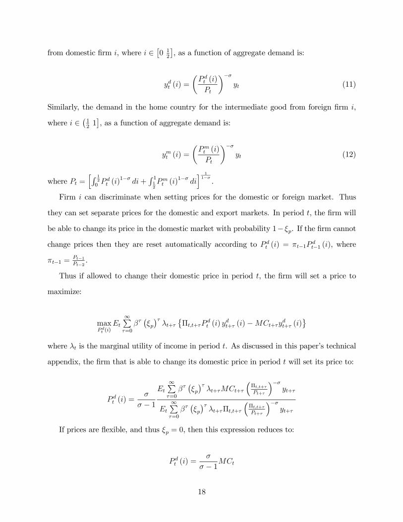
from domestic �rm i, where i 2�0 12

�, as a function of aggregate demand is:

ydt (i) =

�P dt (i)

Pt

���yt (11)

Similarly, the demand in the home country for the intermediate good from foreign �rm i,

where i 2�121�, as a function of aggregate demand is:

ymt (i) =

�Pmt (i)

Pt

���yt (12)

where Pt =hR 1

2

0P dt (i)

1�� di+R 112Pmt (i)

1�� dii 11��.

Firm i can discriminate when setting prices for the domestic or foreign market. Thus

they can set separate prices for the domestic and export markets. In period t, the �rm will

be able to change its price in the domestic market with probability 1� �p. If the �rm cannot

change prices then they are reset automatically according to P dt (i) = �t�1Pdt�1 (i), where

�t�1 =Pt�1Pt�2

.

Thus if allowed to change their domestic price in period t, the �rm will set a price to

maximize:

maxP dt (i)

Et1P�=0

����p���t+�

��t;t+�P

dt (i) y

dt+� (i)�MCt+�y

dt+� (i)

where �t is the marginal utility of income in period t. As discussed in this paper�s technical

appendix, the �rm that is able to change its domestic price in period t will set its price to:

P dt (i) =�

� � 1

Et1P�=0

����p���t+�MCt+�

��t;t+�Pt+�

���yt+�

Et1P�=0

����p���t+��t;t+�

��t;t+�Pt+�

���yt+�

If prices are �exible, and thus �p = 0, then this expression reduces to:

P dt (i) =�

� � 1MCt

18

which says that the �rm will set a price equal to a constant mark-up over marginal cost.

Write the domestic price set by the �rm that can reset prices in period t as ~P dt (i) to

denote that it is an optimal price. Firms that can reset prices in period t will all reset

to the same level, so ~P dt (i) = ~P dt . Substitute this optimal price into the price index Pdt =�

2R 1

2

0

�P dt (i)

�1��di� 11��. Since a �rm has a probability of 1��p of being able to change their

price, then by the law of large numbers in any period 1� �p percent of �rms will reoptimize

prices, and the prices of �p percent of �rms will be automatically reset using the previous

periods in�ation rate. Thus the domestic price index, P dt , can be written as:

P dt =

��p��t�1;tP

dt�1�1��

+�1� �p

� �~P dt

�1��� 11��

The full details of this derivation as well as the derivation for prices set for the foreign

market is located in the appendix.

The �rm hires labor and capital inputs, where Wt is the wage rate paid for labor input

and Rt is the capital rental rate, both of which the �rm takes as given. Furthermore the �rm

must pay their wage bill in advance. To do so they borrow bwct (i) = Wtht (i). The �rm�s

income after paying for capital and labor inputs is:

dft (i) = P dt (i) ydt (i) + P xt (i) y

xt (i)�Wtht (i)�Rtkt (i)� rwct b

wct (i) (13)

where P xt (i) is the export price for the intermediate good from �rm i, and rwct is the interest

rate on working capital loans. Since there is no default risk from lending working capital to

�rms, competition in the banking sector forces the rate on working capital loans down to

the bank�s own cost of capital, rwct = rbt .

The aggregate income from all �rms is returned to households as a lump sum payment,

dft =R n0dft (i) di.

The �rm will choose ht (i) and kt (i) to maximize pro�t in (13) subject to the production

function in (9). The working capital requirement implies that the cost of the labor input is

19

Wt (1 + rwct ) and the cost of the capital input is Rt. Given these prices, the �rm�s demand

for labor and capital inputs are:

ht (i) = (1� �)MCt

Wt (1 + rwct )Yt (i) (14)

kt (i) = �MCtRt

Yt (i)

where MCt =1At

�Wt(1+rwct )

1��

�1�� �Rt�

��.

3.2 Entrepreneurs

Entrepreneurs, indexed j 2�0 12

�, buy capital from capital builders and rent it to �rms. At

the beginning of period t, entrepreneur j has a stock of capital, Kt (j), that he will rent to

�rms in period t at a rental rate Rt. In equilibrium, the aggregate stock of capital supplied

by all domestic entrepreneurs j is equal to the aggregate stock of capital demanded by all

domestic �rms i,R 1

2

0Kt (j) dj =

R 12

0kt (i) di.

Entrepreneurs �nance this stock of capital partially through debt. The entrepreneur

borrows bet (j) from domestic banks and beft (j) from foreign banks to �nance their capital

stock Kt (j). Thus the market value of the assets and liabilities for entrepreneur j at the

beginning of period t are:

Assets: PKt Kt (j)

Liabilities: bet (j) + beft (j)(15)

where PKt is the price of existing capital.

The end of period the value of the non-depreciated capital stock for the average entrepre-

neur is PKt (1� �)Kt. However during the period, the individual entrepreneur j receives an

idiosyncratic draw that a¤ects the relative price of their existing capital, so for entrepreneur

j the end of period value of their non-depreciated capital stock is:

20

!et (j)PKt (1� �)Kt (j)

where !et (j) is a i.i.d. draw from a lognormal distribution on the interval [0;1) with mean

1 and variance �2e.

Since this draw has a mean 1, it has no e¤ect on the aggregate capital stock. It simply

introduces heterogeneity among entrepreneurs, and in any given period a fraction of entre-

preneurs receive a draw that has a large adverse e¤ect on the value of their existing capital

(a small !et (j)) and thus at the end of the period, the value of their liabilities exceeds the

value of their assets.

During the period the entrepreneur rents his capital stock to �rms for a rental rate of Rt.

The entrepreneur pays a net interest rate of ret on loans from domestic banks and reft on loans

from foreign banks. Thus at the end of the period, after the realization of !et (j), the nominal

market value of entrepreneur j�s assets is !et (j)PKt (1� �)Kt (j)+RtKt (j). At the end of the

period the nominal value of the entrepreneur�s liabilities is (1 + ret ) bet (j) +

�1 + reft

�beft (j).

Thus, after the realization of !et (j), entrepreneur j is bankrupt if:

!et (j)PKt (1� �)Kt (j) +RtKt (j) < (1 + r

et ) b

et (j) +

�1 + reft

�beft (j) (16)

Thus the threshold value of !et (j) below which the entrepreneur goes bankrupt in period

t and above which they continue operations is:

�!et =

h1 + (1� �) ret + �reft

ibet (j)+b

eft (j)

Kt(j)�Rt

PKt (1� �)(17)

where � = beft (j)

bet (j)+beft (j)

and DAet (j) =bet (j)+b

eft (j)

Kt(j)is the ratio of the book value of debt to

the book value of assets on an entrepreneur�s balance sheet. The history of individual

entrepreneur j will determine the level of bet (j), beft (j) and Kt (j), but the ratio DAet (j) =

bet (j)+beft (j)

Kt(j)is equal across all entrepreneurs. This is a key result for aggregation, for it implies

that the bankruptcy cuto¤ value �!et does not depend on an entrepreneur�s history. More

21

intuition behind this result is presented at the end of this section and a formal proof is

presented in the appendix.

When deciding how much to lend to entrepreneurs going into next period and at what

rate, banks factor in the fact that if entrepreneur j does not default in period t+1, domestic

creditors receive a return of ret+1 and foreign creditors receive reft+1. If the entrepreneur

defaults, creditors receive a share of the entrepreneur�s remaining assets, less the bankruptcy

cost �e. The threshold value �!et+1 in equation (17) determines whether or not an entrepreneur

goes into default next period. Thus the payo¤ to domestic and foreign creditors conditional

of the realization of the shock !et+1 (j) is:

Payo¤ to domestic creditors:�1 + ret+1

� �bet+1 (j)

�if !et+1 (j) � �!et+1

(1� �) (1� �e)�!et+1 (j) (1� �)PKt+1Kt+1 (j) +Rt+1Kt+1 (j)

�if !et+1 (j) < �!et+1

Payo¤ to foreign creditors:�1 + reft+1

��beft+1 (j)

�if !et+1 (j) � �!et+1

� (1� �e)�!et+1 (j) (1� �)PKt+1Kt+1 (j) +Rt+1Kt+1 (j)

�if !et+1 (j) < �!et+1

(18)

Perfect competition in the banking sector implies that the bank�s expected pro�t is zero.

So the interest rate the (home or foreign) bank charges on physical capital loans, ret+1 or

reft+1, is set such that the expected return, after factoring in the cost of bankruptcy, is equal

to the (home or foreign) bank�s cost of capital, rbt+1 or rb�t+1:

22

For domestic creditors :

�1 + rbt+1

�bet+1 (j) =

Z �!et+1

0

(1� �) (1� �e)

0B@ !et+1 (j) (1� �)PKt+1Kt+1 (j)

+Rt+1Kt+1 (j)

1CA dF�!et+1

�+

Z 1

�!et+1

�1 + ret+1

�bet+1 (j) dF

�!et+1

�For foreign creditors :

�1 + rb�t+1

�beft+1 (j) =

Z �!et+1

0

� (1� �e)

0B@ !et+1 (j) (1� �)PKt+1Kt+1 (j)

+Rt+1Kt+1 (j)

1CA dF�!et+1

�+

Z 1

�!et+1

�1 + reft+1

�beft+1 (j) dF

�!et+1

�where F

�!et+1

�is the c.d.f. of the lognormal distribution of !et+1.

Thus the interest rate charged by banks for physical capital loans is:

1 + ret+1 =

�1 + rbt+1

�1� F

��!et+1

� � (1� �e)hRt+1F

��!et+1

�+ (1� �)PKt+1

R �!et+10

!et+1dF�!et+1

�i�1� F

��!et+1

�� bet+1(j)+beft+1(j)Kt+1(j)

1 + reft+1 =

�1 + rb�t+1

�1� F

��!et+1

� � (1� �e)hRt+1F

��!et+1

�+ (1� �)PKt+1

R �!et+10

!et+1dF�!et+1

�i�1� F

��!et+1

�� bet+1(j)+beft+1(j)Kt+1(j)

where F��!et+1

�is the percent of manufacturing �rms that declare bankruptcy.

Holding all else equal, these interest rates, ret+1 and reft+1, are increasing in F

��!et+1

�. If

there are �nancial frictions in the entrepreneurial sector, F��!et+1

�is increasing in �!et+1. �!

et+1

is increasing in the manufacturing �rm�s debt-asset ratio. Thus when there are �nancial

frictions in the entrepreneurial sector, the interest rate on physical capital loans is increasing

in the level of debt on an entrepreneur�s balance sheet.

The cuto¤value of !et+1 (j) in equation (17) combined with the above equilibrium interest

rates demonstrates the feedback loop associated with �nancial frictions in the entrepreneurial

23

sector. When the price of existing capital, PKt+1 falls, the cuto¤ value �!et+1 rises. This

implies that more �rms will receive draws of !et+1 (j) below this cuto¤ value and be forced

into bankruptcy. When more �rms go into bankruptcy, F��!et+1

�increases, and ret+1 and

reft+1 increase as banks now demand a higher interest rate to compensate for the increased

bankruptcy risk. Higher ret+1 and reft+1 means higher interest expenses and lower pro�t for

the entrepreneur, which leads to a further increase in the cuto¤ value �!et+1.

The end of period net worth for the �rm that survives is the �rm�s pro�t in time t plus

the value of their non-depreciated capital stock:

~N et (j) = rktKt (j)� (1 + ret ) bet (j)�

�1 + reft

�beft (j) + !et (j)P

Kt (1� �)Kt (j)

The �rm will pay a dividend to shareholders of det (j) and begin the next period with

net worth N et+1 (j) = ~N e

t (j) � det (j). For simplicity, and keeping with the convention from

Bernanke, Gertler, and Gilchrist (1999), we assume that det (j) = ' ~N et (j), where ' < 1.8

Firms that declare bankruptcy in period t pay no dividend and drop out of the market, they

are replaced with new �rms, which are endowed with start up capital of �N e. Thus the net

worth of the entrepreneurial sector at the beginning of next period is:

N et+1 =

Z �!et

0

N et+1 (j) dF (�!

et) +

Z 1

�!et

N et+1 (j) dF (�!

et) (19)

= �N eF (�!et) + (1� ')�rktKt � (1 + ret ) bet �

�1 + reft

�beft

�(1� F (�!et ))

+ (1� ')PKt (1� �)Kt

Z 1

�!et

!etdF (�!et)

8Much of the �nancial accelerator literature, including Bernanke, Gertler, and Gilchrist (1999) assumea separate entrepreneurial consumption, although adopt the simplifying assumption that entrepreneurs donot actually choose their consumption level, it is simply a �xed portion of their end of period net worth.However, in this model, cross border dividend �ows are an important part of capital market integration, sowe instead adopt the simplifying assumption that a portion of the entrepreneur�s end of period net worth isrebated to share holders in the form of lump sum dividends, and following the convention from the literature,we simply assume that this portion is �xed.

24

The entrepreneur will acquire capital up to the point where the interest rate on bank

loans is equal to the expected return to holding a unit of capital:

(1� �) ret+1 + �reft+1 = Et

�Rt+1 + !et+1 (j) (1� �)PKt+1

PKt

�Since !et+1 (j) is i.i.d. and Et

�!et+1 (j)

�= 1, the right hand side of the above expression

is the same across all entrepreneurs j, which implies that (1� �) ret+1 + �reft+1 is the same

across all entrepreneurs.

3.3 Capital Builders

The representative capital builder converts �nal goods, given by equation (10), into the

physical capital purchased by entrepreneurs. At the end of period t, the non depreciated

physical capital stock is (1� �)Kt, and the physical capital stock at the beginning of the

next period is Kt+1. The evolution of the physical capital stock is given by:

Kt+1 � (1� �)Kt = �

�ItKt

�Kt

where �0 > 0 and �00 < 0 implying that there are diminishing marginal returns to physical

capital investment. Capital builders purchase �nal goods for investment at a price Pt and

sell existing capital to entrepreneurs at a price PKt . Thus the pro�ts of the representative

capital builder are given by:

dct = PKt (Kt+1 � (1� �)Kt)� PtIt

In a competitive capital building sector, pro�t maximization implies that the relative

price of existing capital is:

PKtPt

=

��0�ItKt

���1

25

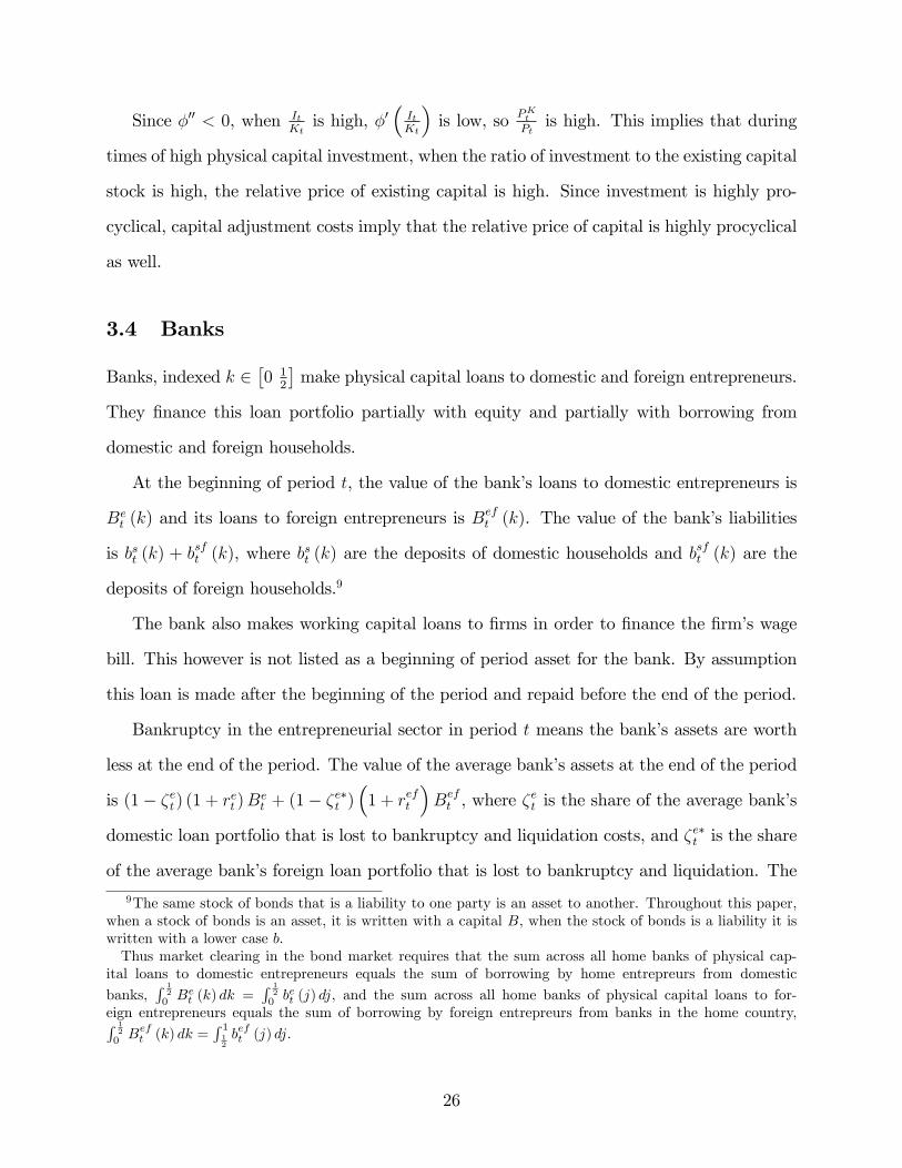
Since �00 < 0, when ItKtis high, �0

�ItKt

�is low, so PKt

Ptis high. This implies that during

times of high physical capital investment, when the ratio of investment to the existing capital

stock is high, the relative price of existing capital is high. Since investment is highly pro-

cyclical, capital adjustment costs imply that the relative price of capital is highly procyclical

as well.

3.4 Banks

Banks, indexed k 2�0 12

�make physical capital loans to domestic and foreign entrepreneurs.

They �nance this loan portfolio partially with equity and partially with borrowing from

domestic and foreign households.

At the beginning of period t, the value of the bank�s loans to domestic entrepreneurs is

Bet (k) and its loans to foreign entrepreneurs is B

eft (k). The value of the bank�s liabilities

is bst (k) + bsft (k), where bst (k) are the deposits of domestic households and b

sft (k) are the

deposits of foreign households.9

The bank also makes working capital loans to �rms in order to �nance the �rm�s wage

bill. This however is not listed as a beginning of period asset for the bank. By assumption

this loan is made after the beginning of the period and repaid before the end of the period.

Bankruptcy in the entrepreneurial sector in period t means the bank�s assets are worth

less at the end of the period. The value of the average bank�s assets at the end of the period

is (1� �et ) (1 + ret )Bet + (1� �e�t )

�1 + reft

�Beft , where �

et is the share of the average bank�s

domestic loan portfolio that is lost to bankruptcy and liquidation costs, and �e�t is the share

of the average bank�s foreign loan portfolio that is lost to bankruptcy and liquidation. The

9The same stock of bonds that is a liability to one party is an asset to another. Throughout this paper,when a stock of bonds is an asset, it is written with a capital B, when the stock of bonds is a liability it iswritten with a lower case b.Thus market clearing in the bond market requires that the sum across all home banks of physical cap-

ital loans to domestic entrepreneurs equals the sum of borrowing by home entrepreurs from domestic

banks,R 1

2

0Bet (k) dk =

R 12

0bet (j) dj, and the sum across all home banks of physical capital loans to for-

eign entrepreneurs equals the sum of borrowing by foreign entrepreurs from banks in the home country,R 12

0Beft (k) dk =

R 112beft (j) dj.

26

asset side of the bank�s balance sheet can be rewritten as:

�1� ��et

�(1 + �ret )

�Bet (k) +Bef

t (k)�

where �Bet (k) = Be

t (k) + Beft (k), �r

et =

Bet (k)

Bet (k)+Beft (k)

ret +Beft (k)

Bet (k)+Beft (k)

reft , and 1 � ��et =

(1��et )(1+ret )Bet (k)+(1��e�t )(1+reft )B

eft (k)

(1+ret )Bet (k)+(1+r

eft )B

eft (k)

.

��et represents the share of the average bank�s portfolio of home and foreign loans that

is lost to bankruptcy and liquidation costs, however banks don�t hold fully diversi�ed loan

portfolios. Some banks may be overexposed to the set of non-performing loans to the entre-

preneurial sector. This overexposure may be due to a regional bias in the bank�s portfolio,

or it may be because a bank has a certain core competency and is therefore overexposed to

a certain sector of the economy.10

The percent of the bank k�s loan portfolio that is lost to bankruptcy or liquidation costs

is !bt (k) ��et , where !

bt (k) is an i.i.d. draw from a lognormal distribution on the interval

h0 1��et

iwith mean 1 and variance �2b .

If bank k receives a large draw !bt (k), it implies that the bank is overexposed to the set

of non-performing loans and may itself face insolvency. The bank is insolvent if the end of

period value of its assets is less than the end of period value of its liabilities:

�1� !bt (k)

��et

�(1 + �ret )

�Bet (k) +Bef

t (k)�<�1 + rbt (k)

� �bst (k) + bsft (k)

�The threshold value of !bt (k) above which bank k is forced to declare bankruptcy and

below which the bank will continue operations is:

�!bt =(1 + �ret )�

�1 + rbt (k)

� bst (k)+bsft (k)

Bet (k)+Beft (k)

��et (1 + �r

et )

(20)

10Like the banks, many of which are now bankrupt or were acquired by healthier rivals, who were overex-posed to the subprime sector of the mortgage market during the recent �nancial crisis.As of early September 2008, the ratio of net subprime assets to total market cap for the four major U.S.

investment banks was: Goldman Sachs-4%, Morgan Stanley-29%, Merrill Lynch-30%, Lehman Brothers-277%. (Potter 2008)

27

Bank k�s history of idiosyncratic draws, !bt (k), thus its history of exposure to non-

preforming sectors of the economy, will determine the levels of Bet (k), B

eft (k), b

st (k), and

bsft (k). However, at the beginning of the period, all banks will have the same ratio of total

debt to total assets, DAbt (k) =bst (k)+b

sft (k)

Bet (k)+Beft (k)

and will have the same cost of capital, rbt (k). This

result is key for the aggregation of balance sheet variables across a continuum of individual

banks, for this implies that the cuto¤ value �!bt is common across all banks. The formal proof

of this claim is presented in the appendix.

When deciding how much to lend to bank k in the next period and at what rate, the

bank�s creditors factor in the fact that if the bank does not default, they receive a gross

interest rate 1 + rbt+1 (k). If bank k defaults, creditors receive nothing.11 Thus the expected

payo¤ to a bank�s creditors conditional on the bank�s exposure to the set of non-preforming

loans is:

�1 + rbt+1 (k)

� �bst+1 (k) + bsft+1 (k)

�if !bt+1 (k) < �!bt+1

0 if !bt+1 (k) � �!bt+1

(21)

Domestic and foreign depositors will extend bank k credit up to the point where the

expected return, after factoring in the probability of default is equal to the risk free rate:

(1 + it+1)�bbt+1 (k) + bbft+1 (k)

�=

Z �!bt+1

0

�1 + rbt+1 (k)

� �bbt+1 (k) + bbft+1 (k)

�dG�!bt+1

�This condition can be used to solve for the interest rate on lending to bank k:

1 + rbt+1 (k) =1 + it+1

G��!bt+1

� (22)

where G��!bt+1

�is the c.d.f. of the lognormal distribution of �!bt+1, and thus measures the

11The assumption that creditors receive nothing in the case of bank default is because the model is latercalibrated such that the spread between the interbank rate, rb, and the risk free rate, i, in the steady state ofthe model is equal to the historical average of the spread between the 3-month Libor and the 3-month T-bill.The Libor is an interbank index rate that is based on the interest rate for unsecured lending to banks.

28

proportion of banks that do not go bankrupt in period t+1. Since DAbt+1 (k) =bst+1(k)+b

sft+1(k)

Bet (k)+Beft (k)

is constant across all banks, the interbank lending rate, and thus banks�cost of capital, is

constant across all banks.

The expressions for the cuto¤ value �!bt+1 in (20) and the interbank interest rate in (22)

show how when there are �nancial frictions in the banking sector, cross border �nancial

integration, in the form of increased cross border lending, can have a positive e¤ect on

cross-country business cycle correlation.

The share of the average domestic bank�s portfolio of home and foreign loans that is

lost to bankruptcy and liquidation costs is ��et , where ��et is simply a weighted average of the

bankruptcy costs on domestic and foreign loans, �et and �e�t , where the weight on the foreign

bankruptcy variable, �e�t is approximately the share of the foreign loans in the bank�s loan

portfolio.

An adverse foreign shock that leads to a fall in foreign output also leads to an increase

in foreign entrepreneurial sector bankruptcies. If home country banks make a signi�cant

number of their loans to foreign entrepreneurs, then loan losses for the average home bank,

��et , increase as well.

A higher proportion of losses for the average home bank lowers the cuto¤value, �!bt . When

the cuto¤ value falls, more home banks will �nd themselves over-exposed to the set of bad

loans and be forced into insolvency. This higher riskiness in the banking sector will cause

the home interbank lending spread to increase. Banks pass on this higher cost of capital to

their borrowers, and thus domestic entrepreneurs �nd their borrowing rates increase, and

they are forced to cut investment and production, because of an adverse shock in the foreign

country. The greater the degree of cross-country borrowing and lending, the greater the

e¤ect of an increase in �e�t on home interbank lending spreads, and thus the treater the

degree of international transmission of the country speci�c productivity shock.

The end of period t net worth of the bank that is not over-exposed to the set of non-

preforming loans and is able to continue operations is:

29

~N bt (k) =

�1� !bt (k)

��et

�(1 + �ret )

�Bet (k) +Bef

t (k)���1 + rbt

� �bst (k) + bsft (k)

�

The bank will pay a dividend to shareholders and begin the next period with a net worth

N bt+1 (k) =

~N bt (k) � dbt (k). As in the case of entrepreneurial sector dividend payouts, we

assume that surviving banks simply pay out dividends equal to a �xed portion of their end

of period net worth, dbt (k) = ' ~N bt (k). Banks that were overexposed to the set of non-

preforming loans and thus were forced into bankruptcy end the period with no net worth

and drop out of the market. They are replaced with new banks that are endowed with start

up capital �N b. Thus the net worth of the entire banking sector at the beginning of next

period is:

N bt+1 =

Z 1

�!bt

�N bdG�!bt�+

Z �!bt

0

~N bt (k) dG

�!bt�

3.5 Households

Households, indexed l 2�0 12

�, supply heterogeneous labor to �rms and consume from their

labor income, interest on savings, and pro�t income from domestic and foreign �rms, entre-

preneurs, capital builders, and banks.

The household maximizes their utility function:

max1Pt=0

�thln (Ct (l))� (Ht (l))

1+�H�H

i(23)

Since we assume complete markets at the national level, we can assume that households

maximize utility subject to one nationwide budget constraint:

30

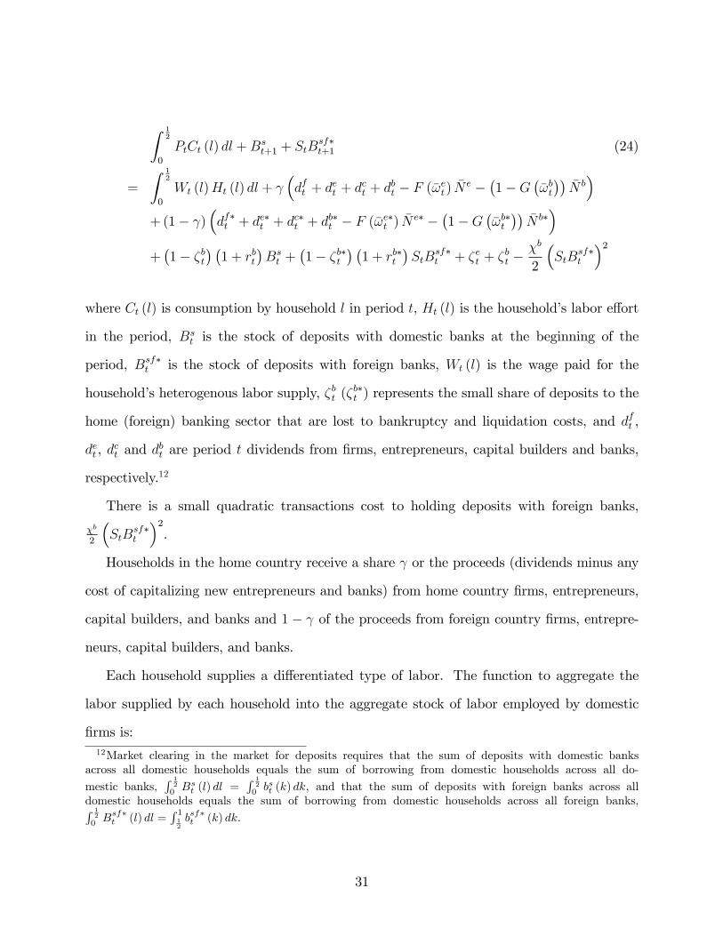
Z 12

0

PtCt (l) dl +Bst+1 + StB

sf�t+1 (24)

=

Z 12

0

Wt (l)Ht (l) dl + �dft + det + dct + dbt � F (�!et)

�N e ��1�G

��!bt���N b�

+(1� )�df�t + de�t + dc�t + db�t � F (�!e�t ) �N

e� ��1�G

��!b�t���N b��

+�1� �bt

� �1 + rbt

�Bst +

�1� �b�t

� �1 + rb�t

�StB

sf�t + �et + �bt �

�b

2

�StB

sf�t

�2where Ct (l) is consumption by household l in period t, Ht (l) is the household�s labor e¤ort

in the period, Bst is the stock of deposits with domestic banks at the beginning of the

period, Bsf�t is the stock of deposits with foreign banks, Wt (l) is the wage paid for the

household�s heterogenous labor supply, �bt (�b�t ) represents the small share of deposits to the

home (foreign) banking sector that are lost to bankruptcy and liquidation costs, and dft ,

det , dct and d

bt are period t dividends from �rms, entrepreneurs, capital builders and banks,

respectively.12

There is a small quadratic transactions cost to holding deposits with foreign banks,

�b

2

�StB

sf�t

�2.

Households in the home country receive a share or the proceeds (dividends minus any

cost of capitalizing new entrepreneurs and banks) from home country �rms, entrepreneurs,

capital builders, and banks and 1� of the proceeds from foreign country �rms, entrepre-

neurs, capital builders, and banks.

Each household supplies a di¤erentiated type of labor. The function to aggregate the

labor supplied by each household into the aggregate stock of labor employed by domestic

�rms is:12Market clearing in the market for deposits requires that the sum of deposits with domestic banks

across all domestic households equals the sum of borrowing from domestic households across all do-

mestic banks,R 1

2

0Bst (l) dl =

R 12

0bst (k) dk, and that the sum of deposits with foreign banks across all

domestic households equals the sum of borrowing from domestic households across all foreign banks,R 12

0Bsf�t (l) dl =

R 112bsf�t (k) dk.

31

Ht =

Z 12

0

Ht (l)��1� dl

! ���1

(25)

where Ht =R n0ht (i) di. Since the household supplies a di¤erentiated type of labor, it faces

a downward sloping labor demand function:

Ht (l) =

�Wt (l)

Wt

���Ht

In any given period, household l faces a probability of 1� �w of being able to reset their

wage, otherwise it is reset automatically according to Wt (l) = �t�1Wt�1 (l).

If household l is allowed to reset their wages in period t they will set a wage to maximize

the expected present value of utility from consumption minus the disutility of labor.

Et1P�=0

�� (�w)�n�t+��t;t+�Wt (l)Ht+� (l)� (Ht+� (l))

1+�H�H

oThus after technical details which are located in the appendix, the household that can

reset wages in period t will choose a wage:

Wt (l)��H

+1=

�

� � 11 + �H�H

(Wt)��H

Et1P�=0

�� (�w)��

Wt+�

�t;t+�Wt

� ��H

+�

(Ht+� )1+�H�H

Et1P�=0

�� (�w)� �t+��t;t+�

�Wt+�

�t;t+�Wt

��Ht+�

If wages are �exible, and thus �w = 0, this expression reduces to:

Wt (l) =�

� � 1

1+�H�H

(Ht)1�H

�t

Thus when wages are �exible the wage rate is equal to a mark-up, ���1 , multiplied by the

marginal disutility of labor, 1+�H�H

(Ht)1�H , divided by the marginal utility of consumption,

�t.

Write the wage rate for the household that can reset wages in period t, Wt (l), as ~Wt (l)

32

to denote it as an optimal wage. Also note that all households that can reset wages in period

t will reset to the same wage rate, so ~Wt (l) = ~Wt.

All households face a probability of (1� �w) of being able to reset their wages in a given

period, so by the law of large numbers (1� �w) of households can reset their wages in a given

period. The wages of the other �w will automatically reset by the previous period�s in�ation

rate.

Substitute ~Wt into the expression for the average wage rate Wt =�R n

0Wt (l)

1�� dl� 11��,

to derive an expression for the evolution of the average wage:

Wt =

��w (�t�1;tWt�1)

1�� + (1� �w)�~Wt

�1��� 11��

3.6 Monetary Policy

The monetary policy instrument is the short term risk free rate, it, which is determined by

the central bank�s Taylor rule function:

it = iss + �i (it�1 � iss) + (1� �i) �p�t +mt (26)

where �t = PtPt�4

, and mt is an exogenous shock to the nominal interest rate.

4 Parameter Values

The model in the previous section is solved with a �rst-order approximation and the results

are found from simulations of the calibrated model. This section will begin by presenting

the basic parameter values used in this calibration. Then we will describe the various types

of exogenous shocks that will drive the simulations of the model and the estimation of these

di¤erent shock processes.

The full list of the model�s parameters and their values is found in table 6.

The �rst seven parameters; the discount factor, the capital depreciation rate, capital�s

33

share of income, the bond adjustment cost parameter, the labor supply elasticity, the elas-

ticity of substitution between goods from di¤erent �rms, and the elasticity of substitution

between labor from di¤erent households are all set to values that are commonly found in the

literature.

The capital adjustment cost parameter, �, describes the curvature of the capital adjust-

ment function ��ItKt

�. It is the elasticity of the relative price of capital with respect to

changes in the investment-capital ratio. This parameter performs the important functions

of lowering the relative volatility of investment and ensuring the procyclicality of the price

of capital. Empirical estimates of this parameter vary, but the value of 0:25 is in the middle

of the range of empirical estimates and ensures that the relative volatility of investment in

the model is near what we see in the data.

The next two parameters in the table are the Calvo price and wage stickiness parameters.

The wage stickiness parameter is chosen such that on average a household adjusts their wages

once a year. The price stickiness parameter implies that prices are a little more �exible than

wages and is taken from the DSGE estimation literature (see e.g. Christiano et al. 2005).

The next set of parameters describe exponents in the central bank�s Taylor rule function.

The interest rate smoothing parameter and the weight on in�ation are all set to values that

are commonly found in the literature.

The next two parameters, � and are the �xed cost in the production of intermediate

goods and the weight on the disutility from labor in the household�s utility function, respec-

tively. These are set to ensure that in the steady state, intermediate goods �rms earn zero

economic pro�t and the household�s labor supply is unity.

The parameter ' measures the �xed portion of a surviving entrepreneur or bank�s net

worth that is rebated to share holders in the form of lump sum dividends. This parameter

is necessary to ensure stationarity in entrepreneur or bank net worth, and thus ensure that

borrowers do not get to the point where they can fully �nance their asset portfolio with

their own net worth. This parameter is simply set to 0:0272 in accordance with the �nancial

34

accelerator model in Bernanke, Gertler, and Gilchrist (1999).

Finally the last three parameters in the table relate to the risk of bankruptcy and liq-

uidation costs in either the banking or entrepreneurial sectors. The parameter �b measures

the steady state level of uncertainty in the �nancial sector. This parameter is determined to

ensure that in the steady state of the model, when banks have a debt-asset ratio of about 0:9,

there is a 13 basis point spread between interbank rates and the risk free rate, the average

spread between the 3-month Libor and the 3-month T-bill from 1984 to 2007.

The cost of liquidation and the idiosyncratic bankruptcy risk in the entrepreneurial sector,

�e and �e are jointly determined. These parameters ensure that in the steady state of the

model, when �rms in the entrepreneurial sector have a debt-asset ratio of 0:5, an entrepreneur

faces a 2% probability of bankruptcy and the steady state spread between the interest rate

on physical capital loans and the bank�s cost of capital is approximately 70 basis points.13

4.1 Exogenous Shock Processes

In this model there are two types of shocks, country speci�c shocks to total factor produc-

tivity (TFP) in (9) and country speci�c monetary policy shocks that appear in the central

bank�s Taylor rule function in (26).

Shocks to TFP are given by:

At = Yt � (1� �) Nt � �Kt

where Yt, Nt, and Kt, are country-speci�c time series of deviations of GDP, employment,

and the capital stocks, from an HP �ltered trend. The series for home and foreign TFP

�uctuations are then used to estimate a VAR(1) process:

13The calibration that entrepreneurs have a steady state debt-asset ratio of about 0:5 and banks havea steady state debt-asset ratio of about 0:9 is based on the historical average debt-asset ratios for U.S.non-�nancial and �nancial �rms as reported in the Federal Reserve�s Flow of Funds Accounts.

35

264 At+1

A�t+1

375 = �A264 At

A�t

375+264 "at

"a�t

375

where A =

264 "at

"a�t

375264 "at

"a�t

3750

is the covariance matrix of the innovations, "at and "a�t .

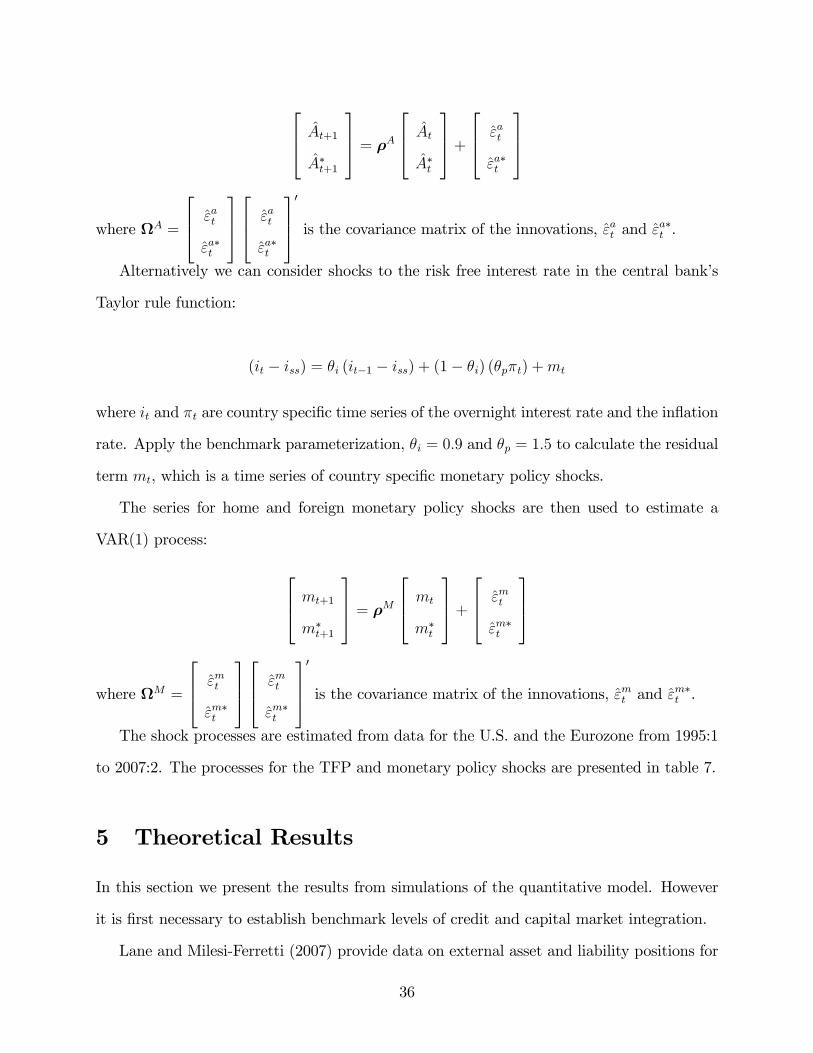
Alternatively we can consider shocks to the risk free interest rate in the central bank�s

Taylor rule function:

(it � iss) = �i (it�1 � iss) + (1� �i) (�p�t) +mt

where it and �t are country speci�c time series of the overnight interest rate and the in�ation

rate. Apply the benchmark parameterization, �i = 0:9 and �p = 1:5 to calculate the residual

term mt, which is a time series of country speci�c monetary policy shocks.

The series for home and foreign monetary policy shocks are then used to estimate a

VAR(1) process:

264 mt+1

m�t+1

375 = �M264 mt

m�t

375+264 "mt

"m�t

375

where M =

264 "mt

"m�t

375264 "mt

"m�t

3750

is the covariance matrix of the innovations, "mt and "m�t .

The shock processes are estimated from data for the U.S. and the Eurozone from 1995:1

to 2007:2. The processes for the TFP and monetary policy shocks are presented in table 7.

5 Theoretical Results

In this section we present the results from simulations of the quantitative model. However

it is �rst necessary to establish benchmark levels of credit and capital market integration.

Lane and Milesi-Ferretti (2007) provide data on external asset and liability positions for

36

a large number of countries. This data is used to construct the Cnfa and Knfa measures

of �nancial integration in section 2. Lane and Milesi-Ferretti report that around the year

2000, the ratio of external capital market liabilities to GDP among industrialized countries

was about 50%. This ratio is reproduced in the model when foreign equities make up about

11% of the household�s equity portfolio.14

The ratio of external credit market liabilities to GDP among industrialized countries is

about 1. This ratio can be reproduced in the model when approximately 24% of a bank�s

loan portfolio is in loans to foreign entrepreneurs.15

We simulate the model under the shock processes described earlier. From the simulated

model we calculate the theoretical correlation between home and foreign GDP. First we

simulate the model to �nd the correlation under the benchmark levels of capital and credit

market integration. Then the correlation is found under the benchmark level of capital

market integration and twice the benchmark level of credit market integration. The di¤erence

between the correlation from the second simulation and that from the �rst simulation is

the e¤ect of increases in credit market integration on cyclical co-movement and is directly

comparable to the coe¢ cient of C in the empirical results in table 5.

Repeating this process but double the level of capital market integration while holding

�xed the level of credit market integration gives the e¤ect of capital market integration of

co-movement and is directly comparable to the coe¢ cient on K in table 5.16

The results from simulations of the model are found in table 8. The �rst row of the

table reports the bilateral output correlation for the model simulated under monetary policy

shocks. The �rst column of the table reports the results from the benchmark parameteri-

zation, the second column reports the results when the level of credit market integration is

doubled, and the third column reports the results when the level of capital market integration

14In terms of the household�s budget constraint in (24), = :11.15In the steady state, bef

be+bef= :24.

16The theoretical simulations speci�cally measure the e¤ect of a change in the stock of extrenal credit orcapital market assets on co-movement. Therefore the theoretical results are most comparable to the resultsfrom the volume based measures of �nancial integration, cpis and nfa, in the top half of table 5.

37

is doubled.

In the model, doubling the level of credit market integration leads to a 9 percentage

point increase in cross-country output correlation and doubling the level of capital market

integration leads to a 9 percentage point decrease. Qualitatively, this is exactly what we see

in the data, and quantitatively, the model can only match about two-thirds of the impact of

�nancial integration that we see in the data.

The second row of the table reports the results from simulations of the model under

monetary policy shocks, but where the �nancial accelerator mechanism in the model has

been "turned o¤". Here the cost of capital for both banks and entrepreneurs is not a

function of debt-asset ratios. In the second row, where balance sheets of both entrepreneurs

and banks are again irrelevant for macroeconomic outcomes, doubling the level of capital

market integration again has a negative e¤ect on bilateral correlation (although smaller than

before). Doubling the level of credit market integration also has a positive e¤ect, but it is

much smaller and close to zero. Thus the empirical results where credit market integration

has a positive e¤ect on bilateral correlation only holds in the model with �nancial accelerator

e¤ects.

The third and fourth rows of the table presents the results from simulations of the model

where business cycles are driven by country-speci�c TFP shocks. Qualitatively, the model

is still able to match the data. Quantitatively, the results are weaker. In the third row,

when the �nancial accelerator is "turned on", doubling the level of credit market integration

leads to about a 1 percentage point increase in bilateral correlation, and doubling the level

of capital market integration leads to about a 2 percentage point decrease.

Table 9 presents the results from various robustness checks. The �rst panel in the table

presents the results from simulations of the model where wages are perfectly �exible, and

thus only intermediate goods prices are sticky. When only prices are sticky, the e¤ect of

doubling the level of �nancial integration is marginally higher, when wages were also sticky,

doubling the level of credit market integration led to a 9 percentage point increase in GDP

38

correlation, now the increase is slightly greater than 10 percentage points. Similarly doubling

the level of capital market integration caused GDP correlation to fall by 9 percentage points

when wages were sticky, now correlation falls by about 10 percentage points under �exible

wages.

The table also presents the results from versions of the model where wages are sticky but

goods prices are �exible, where �rms must pay their wage bill in advance (working capital

channel), where debt contracts are indexed (and thus surprise in�ation does not erode the

real value of debt), and the version of the model that is an international real business cycle

model. These variations have a marginal e¤ect on the impact of doubling the level of credit or

capital market integration on cross-country GDP co-movement, but the masin result that the

model with �nancial frictions can reproduce the positive e¤ect of credit market integration

and the negative e¤ect of capital market integration is unchanged.

6 Summary and Conclusion

This paper shows how international �nancial integration that involves trade in equity and

ownership shares leads to less international business cycle co-movement. This paper also

shows how �nancial integration that involves trade in debt may lead to greater cyclical co-

movement. The negative e¤ect of capital market integration is a common feature of many

international real business cycle models and comes from the wealth e¤ect. The positive e¤ect

of credit market integration is entirely due to balance sheet e¤ects and requires a �nancial

accelerator.

This paper explains why di¤erent types of �nancial integration seem to have had dif-

ferent e¤ects on cross-country business cycle co-movement. Years of international �nancial

integration in the form of equity market integration and cross-border FDI �ows seem to have

resulted in less co-movement and a "decoupling" of the U.S. business cycle from the rest of

the world (Heathcote and Perri 2003), but this "decoupling" trend reversed sharply in the

39

Fall of 2008. A housing bubble and a subprime crisis in the United States and a handful

of other countries quickly spread around the world as banks in countries without a housing

bubble still found themselves exposed to declining house prices and defaults in the United

States.

Relatively little attention has been paid to the e¤ect of �nancial integration on interna-

tional business cycle co-movement (relative to the amount of attention paid to the e¤ect of

trade on co-movement). This is partly because the data is better for trade �ows than for

�nancial �ows, but partly because there seemed to be little consistency in the results. On one

hand �nancial integration seemed to be leading to increased ex-ante risk sharing and thus

made possible the "decoupling" of production cycles, but on the other hand �nancial integra-

tion brought the possibility of �nancial contagion and the international spread of �nancial

panic. This paper shows that when we think of �nancial integration not as one homogenous

set of �nancial �ows, but rather as a heterogenous set, some involving credit constrained par-

ties and some involving non-credit constrained parties, these seemingly inexplicable results

can be explained.

40

References

Aikman, David, and Matthais Paustain, 2006, Bank capital, asset prices, and monetarypolicy, Bank of England Working Paper No. 305.

Allen, Franklin, and Douglas Gale, 2000, Financial contagion, Journal of Political Economy108, 1�33.

Allen, Franklin, Jun Qian, and Meijun Qian, 2005, Law, �nance, and economic growth inchina, Journal of Financial Economics 77, 57�116.

Asdrubali, Pierfedeerico, Bent E. Sørensen, and Oved Yosha, 1996, Channels of interstaterisk sharing, Quarterly Journal of Economics 111, 1081�1110.

Backus, David K., Patrick J. Kehoe, and Finn E. Kydland, 1995, International businesscycles: Theory and evidence, in: T.F. Cooley, ed., Frontiers of Business Cycle Research)331�356.

Balassa, Bela, 1965, Trade liberalization and revealed comparative advantage, ManchesterSchool of Economic and Social Studies 55, 99�123.

Baxter, Marianne, and Mario J. Crucini, 1995, Business cycles and the asset structure offoreign trade, International Economic Review 36, 821�854.

Bernanke, Ben S., Mark Gertler, and Simon Gilchrist, 1999, The �nancial accelerator ina quantitative business cycle framework, in: John B. Taylor, Michael Woodford, eds,Handbook of Macroeconomicsvol. 1 ) 1341�1393.

Calvo, Guillermo A., 1983, Staggered prices in a utility-maximizing framework, Journal ofMonetary Economics 12, 383�398.

Cetorelli, Nicola, and Linda S. Goldberg, 2010, Global banks and international shock trans-mission: Evidence from the crisis, NBER Working Paper No. 15974.

Chen, Nan-Kuang, 2001, Bank net-worth, asset prices, and economic activity, Journal ofMonetary Economics 48, 415�436.

Christiano, Lawrence J., Martin Eichenbaum, and Charles L. Evans, 2005, Nominal rigitiesand the dynamic e¤ects of a shock to monetary policy, Journal of Political Economy113, 1�45.

Clark, Todd, and vanEric Wincoop, 2001, Borders and business cycles, Journal of Interna-tional Economics 55, 59�85.

Curdia, Vasco, and Michael Woodford, 2010, Credit spreads and monetary policy, Journalof Money, Credit, and Banking 42, 3�35.

Davis, Scott, 2010, The adverse feedback loop and the e¤ects of risk in both the real and�nancial sectors, Federal Reserve Bank of Dallas, Globalization and Monetary PolicyInstitute Working Paper No. 66.

41

Dedola, Luca, and Giovanni Lombardo, October 2009, Financial frictions, �nancial integra-tion, and the international propogation of shocks, mimeo.

Devereux, Michael B., and James Yetman, 2010, Leverage constraints and the internationaltransmission of shocks, NBER Working Paper No. 16226.

Dib, Ali, 2010, Banks, credit market frictions, and business cycles, mimeo.

Faia, Ester, 2007, Finance and international business cycles, Journal of Monetary Economics54, 1018�1034.

Frankel, Je¤rey A., and Andrew K. Rose, 1998, The endogeneity of optimum currency areacriteria, The Economic Journal 108, 1009�1025.

Gertler, Mark, and Nobuhiro Kiyotaki, 2010, Financial intermediation and credit policy inbusiness cycle analysis, in: Benjamin M. Friedman, Michael Woodford, eds, Handbookof Monetary Economicsvol. 3 ).

Gertler, Mark, and Peter Karadi, 2011, A model of unconventional monetary policy, Journalof Monetary Economics 58(1), 17�34.

Gilchrist, Simon, Alberto Ortiz, and Egon Zakrajsek, July 2009, Credit risk and the macro-economy: Evidence from an estimated dsge model, mimeo.

Heathcote, Jonathan, and Fabrizio Perri, 2002, Financial autarky and international businesscycles, Journal of Monetary Economics 49, 601�627.

2003, Why has the U.S. economy become less correlated with the rest of the world?,The American Economic Review (Papers and Proceedings) 93, 63�69.

2004, Financial globalization and real regionalization, Journal of Economic Theory119, 207�243.

Hirakata, Naohisa, Nao Sudo, and Kozo Ueda, 2009, Credit conditions of �nancial interme-diaries and entrepreneurs and �nancial accelerators, mimeo.

Holstrom, Bengt, and Jean Tirole, 1997, Financial intermediation, loanable funds, and thereal sector, Quarterly Journal of Economics 112(3), 663�691.

Imbs, Jean, 2004, Trade, �nance, specialization, and synchronization, The Review of Eco-nomics and Statistics 86, 723�734.

2006, The real e¤ects of �nancial integration, Journal of International Economics68, 296�324.

Imbs, Jean, and Romain Wacziarg, 2003, Stages of diversi�cation, The American EconomicReview 93, 63�86.

Kalemli-Ozcan, Sebnem, Bent E. Sørensen, and Oved Yosha, 2001, Economic integration,industrial specialization, and the asymmetry of macroeconomic �uctuations, Journal ofInternational Economics 55, 107�137.

42

2003, Risk sharing and industrial specialization: Regional and international evidence,The American Economic Review 93, 903�918.

Kalemli-Ozcan, Sebnem, Elias Papaioannou, and Jose Luis Peydro, 2009, Financial integra-tion and business cycle synchronization, NBER Working Paper No. 14887.

Kaminsky, Graciela L., and Carmen M. Reinhart, 2000, On crisis, contagion, and confusion,Journal of International Economics 51, 145�168.

Kaminsky, Graciela L., Carmen M. Reinhart, and Carlos A. Vegh, 2003, The unholy trinityof �nancial contagion, NBER Working Paper No. 10061.

Kehoe, Patrick J., and Fabrizio Perri, 2002, International business cycles with endogenousincomplete markets, Econometrica 70, 907�928.

Kollmann, Robert, and Frederic Malherbe, 2011, International �nancial contagion: The roleof banks, ECORE Discussion Paper 2011/1.

Kollmann, Robert, Zeno Enders, and Gernot J. Muller, 2011, Global banking and interna-tional business cycles, European Economic Review 55, 407�426.

Kose, M. Ayhan, Christopher Otrok, and Charles H. Whiteman, 2008a, Understanding theevolution of world business cycles, Journal of International Economics 75(1), 110�130.

Kose, M. Ayhan, Christopher Otrok, and Eswar S. Prasad, 2008b, Global business cycles:Convergence or decoupling, IZA Working Paper No. 3442.

Kose, M. Ayhan, Eswar S. Prasad, and Marco E. Terrones, 2003, How does globalizationa¤ect the synchronization of business cycles, The American Economic Review (Papersand Proceedings) 93, 57�62.

Krugman, Paul, 2008, The international �nancial multiplier, mimeo.

La Porta, Rafael, Lopez-deFlorencio Silanes, Andrei Shleifer, and Robert W. Vishny, 1998,Law and �nance, Journal of Political Economy 106, 1113�1155.

Lane, Philip R., and Gian Maria Milesi-Ferretti, 2007, The external wealth of nations mark ii:Revised and extended estimates of foreign assets and liabilities, 1970-2004, The Journalof International Economics 73, 223�250.

Meh, Cesaire A., and Kevin Moran, 2010, The role of bank capital in the propagation ofshocks, Journal of Economic Dynamics and Control 34(3), 555�576.

Modigliani, Franco, and Merton H. Miller, 1958, The cost of capital, corporation �nance,and the theory of investment, The American Economic Review 48(3), 261�297.

Moto, Ashoka, Lucio Sarno, and Mark P. Taylor, 2007, A cross-country �nancial accelerator:Evidence from north america and europe, Journal of International Money and Finance26, 149�165.

43

Nicita, Alessandro, and Marcelo Olarrenga, 2006, Trade, production, and protection 1976-2004, World Bank Economic Review.

Pistor, Katharina, Martin Raiser, and Stanislaw Gelfer, 2000, Law and �nance in transitioneconomies, Economics of Transition 8, 325�368.

Portes, Richard, and Helene Rey, 2005, The determinats of cross-border equity �ows, Journalof International Economics 65, 269�296.

Potter, Steven, 2008, Subprime Exposure Comparison - Lehman Brothers Files BankruptcyMerrill Lynch Is Sold and Goldman Sachs Better Morgan Stanley, Best SyndicationNews, September 15, 2008.

Stein, Jeremy C., 1998, An adverse-selection model of bank asset and liability managementwith implications for the transmission of monetary policy, The RAND Journal of Eco-nomics 29(3), 466�486.

Taylor, John B., and John C. Williams, 2009, A black swan in the money market, AmericanEconomic Journal: Macroeconomics 1(1), 58�83.

Ueda, Kozo, 2010, Banking globalization and international business cycles, Federal ReserveBank of Dallas, Globalization and Monetary Policy Institute Working Paper No. 58.

van denHeuvel, Skander J., 2009, The bank capital channel of monetary policy, mimeo.

vonPeter, Goetz, 2009, Asset prices and banking distress: A macroeconomic approach, Jour-nal of Financial stability 5, 298�319.

44

A Appendix

This appendix will present some of the more technical derivations in the paper related to

the nominal rigidities and �nancial frictions present in the model. First, section A.1 presents

the list of countries that are used in the empirical regressions. Then, section A.2 presents

the derivations involved with the Calvo style wage and price equations. Finally, section A.3

presents the proofs necessary for aggregation in the presence of �nancial frictions.

A.1 Countries in the estimations

Argentina; Australia; Austria; Belgium-Luxembourg; Brazil; Bulgaria; Canada; Chile; China;

Colombia; Czech Rep.; Denmark; Ecuador; Egypt; Finland; France; Germany; Greece;

Hong Kong; Hungary; India; Indonesia; Ireland; Israel; Italy; Japan; Jordan; Kenya; Ko-

rea; Latvia; Malaysia; Mexico; Netherlands; New Zealand; Nigeria; Norway; Pakistan; Peru;

Philippines; Poland; Portugal; Romania; Russia; Singapore; Slovakia; Slovenia; South Africa;

Spain; Sri Lanka; Sweden; Switzerland; Taiwan; Thailand; Turkey; UK; Uruguay; USA;

Venezuela

A.2 Nominal Rigidities

A.2.1 Sticky Wages

In any given period, household j faces a probability of 1��w of being able to reset their wage,

otherwise it is reset automatically according to Wt (l) = �t�1Wt�1 (l), where �t�1 =Pt�1Pt�2

.

If household j is allowed to reset their wages in period t they will set a wage to maximize

the expected present value of utility from consumption minus the disutility of labor.

Et1P�=0

�� (�w)�n�t+��t;t+�Wt (l)Ht+� (l)� (Ht+� (l))

1+�H�H

o(27)

where �t+� is the marginal utility of consumption in period t+ � .17

17We assume complete contingent claims markets among households within a country. This implies that

45

�t;t+� =

8><>: 1 if � = 0

�t+��1�t;t+��1 if � > 0

The imperfect combination of labor from di¤erent households is described in (25). Use

this function to derive the demand function for labor from a speci�c household:

Ht (l) =

�Wt (l)

Wt

���Ht (28)

where Wt =�R n

0Wt (l)

1�� dl� 11��

is the average wage across households, and Ht is aggregate

labor supplied by all households.

Substitute the labor demand function into the maximization problem to express the

maximization problem as a function of one choice variable, the wage rate, Wt (l):

Et1P�=0

�� (�w)�

8<:�t+��t;t+�Wt (l)

��t;t+�Wt (l)

Wt+�

���Ht+� �

��t;t+�Wt (l)

Wt+�

���Ht+�

! 1+�H�H

9=;After some rearranging, the �rst order condition of this problem is:

Wt (l)��N

+1=

�

� � 11 + �H�H

(Wt)��H

Et1P�=0

�� (�w)��

Wt+�

�t;t+�Wt

� ��H

+� �Ht+�

� 1+�H�H

Et1P�=0

�� (�w)� �t+��t;t+�

�Wt+�

�t;t+�Wt

��Ht+�

If wages are �exible, and thus �w = 0, this expression reduces to:

Wt (l) =�

� � 1

1+�H�H

(Ht)1�H

�t

Thus when wages are �exible the wage rate is equal to a mark-up, �(��1) , multiplied by the

the marginal utility of consumption is the same across all households within a country, regardless of theirincome. Therefore the total utility from the consumption of labor income in any period is simply the countryspeci�c marginal utility of comsumption, �t, multiplied by the household�s labor income, Wt (l)Nt (l).

46

marginal disutility of labor, 1+�H�H

(Ht)1�H , divided by the marginal utility of consumption,

�t.

Write the wage rate for the household that can reset wages in period t, Wt (l), as ~Wt (l)

to denote it as an optimal wage. Also note that all households that can reset wages in period

t will reset to the same wage rate, so ~Wt (l) = ~Wt.

All households face a probability of (1� �w) of being able to reset their wages in a given

period, so by the law of large numbers (1� �w) of households can reset their wages in a given

period. The wages of the other �w will automatically reset by the previous periods in�ation

rate.

So substitute ~Wt into the expression for the average wage rateWt =�R n

0Wt (l)

1�� dl� 11��,

to derive an expression for the evolution of the average wage:

Wt =

��w (�t�1;tWt�1)

1�� + (1� �w)�~Wt

�1��� 11��

A.2.2 Sticky Output Prices

Domestic Prices In the model, intermediate goods prices are sticky. Intermediate goods

�rms can set separate domestic and export prices.

In period t, the �rm will be able to change it�s price in the domestic market with prob-

ability 1� �p. If the �rm cannot change prices then they are reset automatically according

to P dt (i) = �t�1Pdt�1 (i).

The �rm that can reset prices in period t will choose P dt (i) to maximize discounted future

pro�ts:

maxP dt (i)

Et1P�=0

����p���t+�

��t;t+�P

dt (i) y

dt+� (i)�MCt+�y

dt+� (i)

where MCt+� is marginal cost of production in period t+ � .

The �rm�s domestic demand is given in (11). Substitute this demand function into the

maximization problem to express this problem as a function of one choice variable, Pt (i):

47

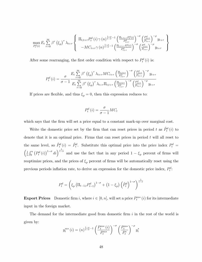
maxP dt (i)

Et1P�=0

����p���t+�

8><>:�t;t+�P

dt (i) (n)

1��1���1

��t;t+�P dt (i)

P dt+�

��� �P dt+�Pt+�

���yt+�

�MCt+� (n)1��1���1

��t;t+�P dt (i)

P dt+�

��� �P dt+�Pt+�

���yt+�

9>=>;After some rearranging, the �rst order condition with respect to P dt (i) is:

P dt (i) =�

� � 1

Et1P�=0

����p���t+�MCt+�

��t;t+�P dt+�

��� �P dt+�Pt+�

���yt+�

Et1P�=0

����p���t+��t;t+�

��t;t+�P dt+�

��� �P dt+�Pt+�

���yt+�

If prices are �exible, and thus �p = 0, then this expression reduces to:

P dt (i) =�

� � 1MCt

which says that the �rm will set a price equal to a constant mark-up over marginal cost.

Write the domestic price set by the �rm that can reset prices in period t as ~P dt (i) to

denote that it is an optimal price. Firms that can reset prices in period t will all reset to

the same level, so ~P dt (i) =~P dt . Substitute this optimal price into the price index P

dt =�

1n

R n0

�P dt (i)

�1��di� 11��

and use the fact that in any period 1 � �p percent of �rms will

reoptimize prices, and the prices of �p percent of �rms will be automatically reset using the

previous periods in�ation rate, to derive an expression for the domestic price index, P dt :

P dt =

��p��t�1;tP

dt�1�1��

+�1� �p

� �~P dt

�1��� 11��

Export Prices Domestic �rm i, where i 2 [0; n], will set a price Pm�t (i) for its intermediate

input in the foreign market.

The demand for the intermediate good from domestic �rm i in the rest of the world is

given by:

ym�t (i) = (n)1��1���1

�Pm�t (i)

Pm�t

��� �Pm�t

P �t

���y�t

48

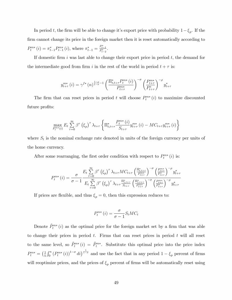
In period t, the �rm will be able to change it�s export price with probability 1��p. If the

�rm cannot change its price in the foreign market then it is reset automatically according to

Pm�t (i) = ��t�1Pm�t�1 (i), where �

�t�1 =

P �t�1P �t�2

.

If domestic �rm i was last able to change their export price in period t, the demand for

the intermediate good from �rm i in the rest of the world in period t+ � is:

ym�t+� (i) = f� (n)1��1���1

���t;t+�P

m�t (i)

Pm�t+�

��� �Pm�t+�

P �t+�

���y�t+�

The �rm that can reset prices in period t will choose Pm�t (i) to maximize discounted

future pro�ts:

maxPm�t (i)

Et1P�=0

����p���t+�

���t;t+�

Pm�t (i)

St+�ym�t+� (i)�MCt+�y

m�t+� (i)

�where St is the nominal exchange rate denoted in units of the foreign currency per units of

the home currency.

After some rearranging, the �rst order condition with respect to Pm�t (i) is:

Pm�t (i) =�

� � 1

Et1P�=0

����p���t+�MCt+�

���t;t+�Pm�t+�

��� �Pm�t+�

P �t+�

���y�t+�

Et1P�=0

����p���t+�

��t;t+�St+�

���t;t+�Pm�t+�

��� �Pm�t+�

P �t+�

���y�t+�

If prices are �exible, and thus �p = 0, then this expression reduces to:

Pm�t (i) =�

� � 1StMCt

Denote ~Pm�t (i) as the optimal price for the foreign market set by a �rm that was able

to change their prices in period t. Firms that can reset prices in period t will all reset

to the same level, so ~Pm�t (i) = ~Pm�t . Substitute this optimal price into the price index

Pm�t =�1n

R n0(Pm�t (i))1�� di

� 11�� and use the fact that in any period 1� �p percent of �rms

will reoptimize prices, and the prices of �p percent of �rms will be automatically reset using

49

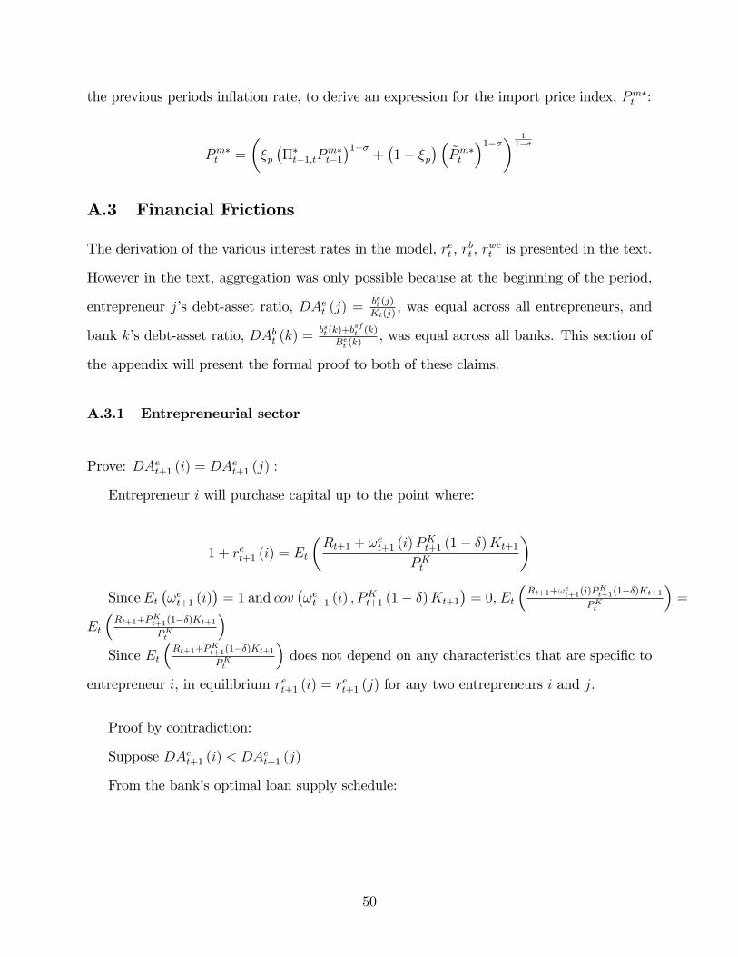
the previous periods in�ation rate, to derive an expression for the import price index, Pm�t :

Pm�t =

��p���t�1;tP

m�t�1�1��

+�1� �p

� �~Pm�t

�1��� 11��

A.3 Financial Frictions

The derivation of the various interest rates in the model, ret , rbt , r

wct is presented in the text.

However in the text, aggregation was only possible because at the beginning of the period,

entrepreneur j�s debt-asset ratio, DAet (j) =bet (j)

Kt(j), was equal across all entrepreneurs, and

bank k�s debt-asset ratio, DAbt (k) =bst (k)+b

sft (k)

Bet (k), was equal across all banks. This section of

the appendix will present the formal proof to both of these claims.

A.3.1 Entrepreneurial sector

Prove: DAet+1 (i) = DAet+1 (j) :

Entrepreneur i will purchase capital up to the point where:

1 + ret+1 (i) = Et

�Rt+1 + !et+1 (i)P

Kt+1 (1� �)Kt+1

PKt

�SinceEt

�!et+1 (i)

�= 1 and cov

�!et+1 (i) ; P

Kt+1 (1� �)Kt+1

�= 0, Et

�Rt+1+!et+1(i)P

Kt+1(1��)Kt+1

PKt

�=

Et

�Rt+1+PKt+1(1��)Kt+1

PKt

�Since Et

�Rt+1+PKt+1(1��)Kt+1

PKt

�does not depend on any characteristics that are speci�c to

entrepreneur i, in equilibrium ret+1 (i) = ret+1 (j) for any two entrepreneurs i and j.

Proof by contradiction:

Suppose DAet+1 (i) < DAet+1 (j)

From the bank�s optimal loan supply schedule:

50

1+ret+1 (j) =

�1 + rbt+1

�1� F

��!et+1 (j)

��(1� �e)hRt+1F

��!et+1 (j)

�+ (1� �)PKt

R �!et+1(j)0

!et+1dF�!et+1

�i�1� F

��!et+1 (j)

�� bet+1(j)

Kt+1(j)

where

�!et+1 (j) =

�1 + ret+1

� bet+1(j)

Kt+1(j)�Rt+1

PKt+1 (1� �)

If DAet+1 (i) < DAet+1 (j), thenbet (i)

Kt(i)<

bet (j)

Kt(j), so �!et (i) < �!et (j) and r

et (i) < ret (j).

This contradicts with the earlier equilibrium condition that ret+1 (i) = ret+1 (j), thus

DAet+1 (i) � DAet+1 (j) and since the choice of i and j where arbitrary the only possible

equilibrium is one where DAet+1 (i) = DAet+1 (j).

A.3.2 Banking sector

Prove DAbt+1 (i) = DAbt+1 (j) :

Bank i will make loans up to the point where:

1 + rbt+1 (i) = Et��1� !bt+1 (k) �

et+1

� �1 + ret+1

�Bet+1 (i)

�Since !bt+1 (i) is i.i.d. and Et

�!bt+1 (i)

�= 1, Et

��1� !bt+1 (k) �

et+1

� �1 + ret+1

�Bet+1 (i)

�=

Et��1� �et+1

� �1 + ret+1

�Bet+1 (i)

�Thus rbt+1 (i) = rbt+1 (j) for any two banks i and j.

Proof by contradiction:

Suppose DAbt+1 (i) < DAbt+1 (j)

From the equilibrium condition that determines how much credit is extended to a bank:

51

1 + rbt+1 (i) =1 + it+1

G��!bt�

where

�!bt+1 (i) =

�1 + ret+1

���1 + rbt+1 (i)

� bst+1(i)+bsft+1(i)Bet+1(i)

�et+1�1 + ret+1

�If DAbt+1 (i) < DAbt+1 (j) then

bst+1(i)+bsft+1(i)

Bet+1(i)<

bst+1(j)+bsft+1(j)

Bet+1(j), so �!bt+1 (i) > �!bt+1 (j), so

rbt+1 (i) < rbt+1 (j).

This contradicts with the earlier equilibrium condition that rbt+1 (i) = rbt+1 (j), thus

DAbt+1 (i) � DAbt+1 (j) and since the choice of i and j where arbitrary the only possible

equilibrium is one where DAbt+1 (i) = DAbt+1 (j).

52

Table 1: Some descriptive statistics for the various measures of credit and capital marketintegration

Variable Mean St. Dev. Minimum MaximumCcpis 3:18� 10�3 9:87� 10�3 9:63� 10�10 (ESP-IND) 0:100 (IRL-GBR)Kcpis 1:79� 10�3 5:58� 10�3 2:27� 10�10 (JPN-ROM) 0:060 (USA-GBR)Cnfa 0:381 0:416 3:36� 10�5 (NLD-ESP) 2:158 (IRL-JOR)Knfa 0:245 0:268 3:46� 10�4 (RUS-IDN) 1:841 (IRL-SWE)Cmad 0:076 0:048 3:86� 10�3 (DEU-PRT) 0:348 (TUR-JPN)Kmad 0:071 0:022 0:022 (NLD-FRA) 0:150 (TUR-IDN)Crs 0:086 0:093 4:53� 10�5 (ESP-HUN) 0:689 (IDN-NGA)Krs 0:037 0:026 5:90� 10�5 (SVN-PAK) 0:135 (PER-EGY)

Table 2: Unconditional correlations between the various measures of credit and capitalmarket integration

Ccpis Kcpis Cnfa Knfa Cmad Kmad Crs Krs

Ccpis 1Kcpis 0:721 1Cnfa 0:127 0:131 1Knfa 0:187 0:187 0:537 1Cmad �0:146 �0:093 0:036 0:007 1Kmad �0:144 �0:130 �0:005 0:059 0:626 1Crs 0:006 0:033 0:031 �0:047 �0:118 �0:202 1Krs �0:112 �0:054 0:007 �0:077 �0:014 �0:022 0:052 1

Table 3: Some descriptive statistics for the aggregate endogenous variables in the regressionmodel

Variable Mean St. Dev. Minimum Maximum� 0:1343 0:4501 �0:9448 (ESP-CHN) 0:9784 (IRL-PRT)

F cpis 4:9� 10�3 0:0143 1:9� 10�9 (NZL-MEX) 0:1543 (IRL-GBR)F nfa 0:6260 0:6034 0:0061 (SVN-URY) 3:7122 (IRL-SWE)Fmad 0:1474 0:0643 0:0294 (NLD-FRA) 0:4904 (JPN-TUR)F rs 0:1235 0:0985 6:9� 10�4 (FRA-SVN) 0:8192 (IDN-NGA)T 2:1� 10�3 7:8� 10�3 1:2� 10�7 (SGP-IDN) 0:2268 (SGP-MYS)S 0:1567 0:0741 0:0363 (USA-GBR) 0:4211 (SGP-LKA)

53

Table 4: Unconditional correlations between the aggregate endogenous variables in the re-gression model

� F cpis F nfa Fmad F rs T S� 1

F cpis 0:221 1F nfa �0:056 0:183 1Fmad �0:090 �0:147 0:027 1F rs 0:072 �0:010 �0:007 �0:157 1T 0:178 0:363 0:065 0:016 �0:006 1S �0:078 0:006 0:472 0:083 �0:002 0:057 1

54

Table5:Resultsfrom

thecross-sectionalregressionofbusinesscyclecorrelationon�nancialintegration,tradeintegrationand

industrialspecialization.

CPIS

NFA

OLS

GMM

OLS

GMM

F�0:039��

0:073

F0:000

�0:020��

(0:014)

(0:064)

(0:005)

(0:009)

C�0:003

0:136��

C0:004

0:159��

(0:009)

(0:047)

(0:005)

(0:026)

K�0:032��

�0:284��

K�0:005

�0:144��

(0:009)

(0:046)

(0:005)

(0:022)

T0:051��

0:052��

0:002

0:096��

T0:064��

0:068��

0:112��

0:078��

(0:007)

(0:007)

(0:013)

(0:015)

(0:014)

(0:014)

(0:029)

(0:030)

S�0:087��

�0:092��

�1:136��

�0:356�

S�0:129��

�0:128��

�0:541��

�0:611��

(0:027)

(0:026)

(0:156)

(0:184)

(0:031)

(0:031)

(0:155)

(0:159)

MAD

RS

OLS

GMM

OLS

GMM

F�0:142��

0:100

F0:056��

0:258��

(0:035)

(0:086)

(0:014)

(0:073)

C�0:067��

�0:737��

C0:006

0:190��

(0:025)

(0:088)

(0:009)

(0:058)

K�0:105�

1:046��

K0:050��

�0:201��

(0:055)

(0:131)

(0:011)

(0:059)

T0:070��

0:066��

0:147��

0:213��

T0:050��

0:054��

0:024��

�0:039��

(0:011)

(0:011)

(0:020)

(0:022)

(0:006)

(0:007)

(0:012)

(0:019)

S�0:084��

�0:079��

�0:644��

0:700��

S�0:114��

�0:129��

�1:070��

�1:248��

(0:031)

(0:032)

(0:139)

(0:191)

(0:025)

(0:025)

(0:107)

(0:115)

Notes:Robuststandarderrorsarewritteninparenthesis.**impliessigni�cantatthe5%

level,*impliessigni�canceat

the10%level.F,C,K,T,Sarethenaturallogsofthevariableslistedinthetext.

55

Table 6: Benchmark Parameter Values

Symbol Value Description� 0:99 discount factor� 0:025 depreciation rate� 0:36 capital�s share of income�b 0:01 cost of adjusting foreign bond holdings�n 1 labor supply elasticity� 10 substitution elasticity across goods from domestic �rms� 21 substitution elasticity across di¤erentiated labor inputs� 0:25 capital adjustment cost parameter�p 0:62 probability that a �rm cannot change prices in the current period�w 0:75 probability that a worker cannot change wages in the current period�i 0:9 interest rate smoothing parameter�p 1:5 weight on in�ation in the Taylor rule� 0:308 �xed cost in production 0:380 coe¢ cient on labor e¤ort in the utility function' 0:0272 portion of net worth that is rebated to households as dividends�b 1:110 standard deviation of idiosyncratic bank shocks�e 0:275 cost of liquidation in the entrepreneurial sector�e 0:335 standard deviation of idiosyncratic entrepreneur shocks

Table 7: Shock Processes used in the simulation

TFP Shocks:

�A =

�0:775 0:0990:099 0:775

�A = 10�5

�3:747 0:1310:131 3:747

�Monetary Policy Shocks:

�M =

�0:013 0:0150:015 0:013

�M = 10�5

�1:141 0:5920:592 1:141

�

Table 8: The model�s predictions for the e¤ect of credit and capital market integration onbusiness cycle co-movement

Bilateral output correlation:Benchmark 2� C 2�K

Monetary shock 0:542 0:629 0:457Monetary shock (No FA) 0:454 0:467 0:409Productivity shock 0:686 0:694 0:670

Productivity shock (No FA) 0:726 0:736 0:714

56

Table 9: The model�s predictions for the e¤ect of credit and capital market integration onbusiness cycle co-movement under alternative versions of the model

Bilateral output correlation:Benchmark 2� C 2�K

Flexible WagesMonetary shock 0:625 0:728 0:531Monetary shock (No FA) 0:437 0:459 0:387Productivity shock 0:559 0:567 0:541Productivity shock (No FA) 0:602 0:613 0:587

Flexible PricesMonetary shock 0:548 0:624 0:468Monetary shock (No FA) 0:445 0:429 0:407Productivity shock 0:528 0:533 0:521Productivity shock (No FA) 0:579 0:585 0:574

Working CapitalMonetary shock 0:546 0:634 0:465Monetary shock (No FA) 0:466 0:480 0:424Productivity shock 0:708 0:716 0:695Productivity shock (No FA) 0:745 0:755 0:736

Indexed BondsMonetary shock 0:524 0:598 0:454Monetary shock (No FA) 0:457 0:472 0:420Productivity shock 0:690 0:702 0:672Productivity shock (No FA) 0:725 0:736 0:713

IRBCMonetary shock N=A N=A N=AMonetary shock (No FA) N=A N=A N=AProductivity shock 0:474 0:489 0:459Productivity shock (No FA) 0:499 0:506 0:489

57