Financial Entanglement: A Theory of IncompleteIntegration, Leverage, Crashes, and Contagion∗

Nicolae GarleanuUC Berkeley-Haas, NBER, and CEPR

Stavros PanageasUniversity of Chicago, Booth School of Business and NBER

Jianfeng YuUniversity of Minnesota, Carlson School of Business

June 2014

Abstract

We propose a unified model of limited market integration, asset-price determination,leveraging, and contagion. Investors and firms are located on a circle, and access tomarkets involves participation costs that increase with distance. Due to a complemen-tarity between participation and leverage decisions, the market equilibrium may exhibitdiverse leverage and participation choices across investors, even though investors areex-ante identical. Small changes in market-access costs can cause a change in the typeof equilibrium and lead to discontinuous price changes, de-leveraging, and portfolio-flow reversals. Moreover, the market is subject to contagion, in that an adverse shockto investors in a subset of locations affects prices everywhere.

Keywords: Financial frictions, Market fragmentation, Leverage, Crashes, ContagionJEL Classification: G01, G12

∗We are grateful for comments and suggestions from Saki Bigio, Xavier Gabaix, Douglas Gale, MichaelGallmeyer, Arvind Krishnamurthy, Anna Pavlova, Lasse Pedersen, Alp Simsek, Andrzej Skrzypacz, WeiXiong, Adam Zawadowski, three anonymous referees, as well as participants at the AFA, NBER AP, NBER SIMacro-Finance (ME), Minnesota Macro-AP conference, Studienzentrum Gerzensee, the Cowles FoundationGE conference, LBS Four nations cup, Wharton Conference on Liquidity and Financial Crises, and theFinance Theory Group conferences, and seminar audiences at Univ. of Alberta, Univ. of Birmingham,Boston University, Chicago Booth, Columbia Business School, Erasmus University, Hanken, HEC Paris,Univ. of Hong Kong, HKUST, Imperial College, INSEAD, LBS, LSE, Univ. of North Carolina, Stanford-GSB, Tilburg, Vanderbilt, Warwick Business School, Univ. of Washington, Yale SOM.

1 Introduction

There is a substantial body of empirical literature (described in detail in the next section)

concluding that market integration is limited and risk sharing is imperfect. In particular,

a) capital tends to stay “close” to its origin, b) reward for risk reflects — at least partially

— “local” factors that one would expect to be diversifiable, and c) reductions in capital

flows and the extent of market integration tend to coincide with substantial increases in risk

premia and leverage reductions.

Motivated by these findings, we propose a tractable theoretical framework that offers

a unified view of asset-price determination, endogenous market fragmentation, contagion

across seemingly unrelated markets, diversity of observed investment strategies, and de-

leveraging.

The model features a continuum of investors and financial markets located on a circle.

Investors are endowed with shares of a risky firm domiciled at their location and traded at

the same location. The dividends of this security are closely correlated with dividends of

securities located in nearby locations and less correlated with securities in distant locations.

Even though securities in more distant locations offer greater benefits from the perspective of

diversification and risk allocation, participation in such markets involves costs that grow with

the distance from the current location. Such costs are reflective of the fact that informational

frictions are likely to grow as investors participate in progressively more unfamiliar markets.

Indeed, inside our model distance on the circle should not be viewed narrowly as geographical

distance. For our purposes, distance is a broad measure parametrizing a tradeoff between

the cost of overcoming frictions in accessing various asset classes and the diversification

benefits offered by these asset classes. Alongside the risky markets, investors have access to

a zero-net-supply bond market.

Because access to financial markets is subject to frictions, the market equilibrium features

limited integration. Investors from nearby locations, who face similar cost structures, choose

to participate on arcs of the circle that feature a high degree of overlap. Even though there

may be many assets with no common investor, this overlap renders all markets (indirectly)

“entangled.”

1

In such a framework, we examine four sets of issues: a) the determination of asset prices

in light of limited market integration; b) the structure of optimal investment strategies, i.e.,

arcs of participation, leverage, and risky-asset positions chosen by investors; c) the effect of

changes to the financial technology (i.e., the magnitude of market-access costs); and d) the

propagation of “local” shocks to the financial technology. We summarize our findings about

each of the four issues in turn.

a) Limited market integration implies that investors are over-exposed to the risks of

locations in their vicinity. Consequently, risk premia are higher than they would be in a

frictionless world. An important aspect of the analysis is that the magnitudes of risk premia

and of portfolio flows are tightly linked and reflect the extent of market integration.

b) Although investors in any given location are identical in every respect, their investment

strategies may be diverse with some investors choosing high-leverage strategies and increased

extent of participation in risky markets, and others choosing unleveraged, low-participation

strategies.

The intuition for this finding is that leverage and participation decisions are complements.

For a given level of risk premia, participating in more markets increases the maximum Sharpe

ratio attainable, which induces investors to take more leverage. Since leverage increases

the overall variance of the portfolio, it increases the marginal benefit of further market

participation and diversification. This complementarity between participation and leverage

decisions makes the problem of choosing the optimal participation arc a non-concave problem

with (possibly) multiple local optima. As is commonly the case in situations where investors

maximize non-concave problems, a symmetric equilibrium (whereby all investors adopt the

same policies) may fail to exist, and the only equilibrium is asymmetric. It is noteworthy

that the non-concavities arise even when the participation costs are convex.

This implication of the model is consistent with the diversity of investment strategies

offered to investors by, say, mutual funds and hedge funds. More importantly, it shows that

portfolio leverage may arise endogenously in fragmented markets, without requiring inherent

differences between investors.

c) An illustration of the consequences of the complementarity between the breadth of

participation and leverage is provided by the introduction of borrowing limits, e.g., via

2

margin constraints.1 In such a situation, different types of equilibria may coexist, generating

fragility. For instance, marginal variations in participation costs may cause the type of

equilibrium to change, causing discontinuous reactions in prices, capital flows, and leverage.

The intuition is as follows. Absent leverage constraints, broad-participation decisions

by different investors are substitutes: The less other investors participate, the lower the

prices of risky assets, and thus the higher an individual investor’s incentive to take leverage

and participate broadly in markets. A binding leverage constraint changes the situation

significantly. In this case, the lower risky-asset prices necessitate a lower leverage, i.e., a

reduction in the extent to which one can take advantage of an access to diversified portfolios.

The consequence is that the incentive to participate broadly is diminished, relative to the

no-constraint case, by other investors’ non-participation. This complementarity may be so

strong that multiple equilibria, featuring distinct prices, extents of integration, and aggregate

leverage, can co-exist: If prices are low, then leverage is constrained to be low and there isn’t

enough incentive to participate broadly, justifying low prices. If prices are high, then agents

can leverage sufficiently to justify paying for broad participation, which supports high prices.

d) The fact that markets are only partially integrated may strengthen the interdependence

of the prices of risky securities in different locations. We present an example where the

financial technology “breaks down” (i.e., the participation costs rise to infinity) only in a

subset of locations — we refer to them as the “affected” locations. We show that such an

event pushes prices in almost all locations downward. This is true even for locations that

are not connected with the affected locations through asset trade and also have negative

dividend correlation with them.

The intuition for this finding is as follows. As a direct effect of the shock in the affected

regions, investors in affected locations stop investing in risky markets in their vicinity. Con-

sequently, prices in these locations fall so as to attract demand from neighboring unaffected

locations. The portfolio reallocation in these neighboring locations happens away from other,

farther locations, resulting in weaker demand in these farther locations, necessitating price

drops in these locations as well, so as to attract demand from locations neighboring the

neighboring locations, etc.

1In Appendix D we consider alternative formulations of borrowing frictions, motivated by limited liability.

3

The extent of price drops required to compensate investors for tilting their portfolios to

absorb local risks depends on the extent of their overall participation in risky markets. If

the extent of their participation is small, so that their portfolio is heavily exposed to risks

in their vicinity, then a tilt towards a nearby location requires a higher compensation. By

contrast, if investors’ portfolios are invested across a broad range of locations, then they are

more willing to absorb risks in their vicinity. Hence, somewhat surprisingly, the higher the

degree of market integration, the lower the price drop in response to a local participation

shock (and vice-versa).2

In summary, the paper offers a unified framework to study several financial-market phe-

nomena as a result of (endogenous) market segmentation. Besides the specific applications

that we consider, which are meant to illustrate the structure of our framework, we be-

lieve that the paper also makes a technical contribution; it provides a particularly tractable

framework to study the numerous instances in economics where frictions prevent optimal

risk diversification and capital allocation across asset classes.

Our work is related to several strands of theoretical and empirical literature. We discuss

connections to the theoretical literature here and postpone a discussion of related empirical

literature for the next section.

Through its focus on incomplete participation by all agents, our paper is related to the

seminal contribution of Merton (1987) and the studies inspired by it. We endogenize the

degree of participation, and choose a specific asset-universe structure. Circular structures

have been repeatedly used in a variety of applications from location models in industrial

organization (Salop (1979)) to the literature on financial networks.3 From a technical per-

spective, our paper proposes a novel and quite tractable structure to model risky payoffs

continuously distributed on a circle. The paper also differs from the financial-network litera-

ture in setup and questions addressed. Specifically, we study a relatively standard Walrasian

exchange economy with (endogenously) limited participation, while that literature typically

2Interestingly, albeit in a completely different setting, Allen and Gale (2000) also finds that contagion ismore severe when financial interconnectivity — between deposit-taking institutions, in that model — is low.

3An indicative and incomplete listing of papers studying networks, and in particular circular ones, infinance includes Allen and Gale (2000), Freixas et al. (2000), Allen et al. (2012), Caballero and Simsek(2012), Acemoglu et al. (2013), and Zawadowski (2013). Allen and Babus (2009) offers a survey of theliterature.

4

concentrates on banking issues, network externalities, etc.

Allen and Gale (2004a,b) and Carletti and Leonello (2012) provide examples of mixed

equilibria whereby banks — faced with the possibility of runs — may choose different strate-

gies anticipating trading (of loans) with each other at a subsequent date. The source of

asymmetric equilibria in our paper is different, and more closely related to Aumann (1966),

whose analysis covers Walrasian setups (without idiosyncratic liquidity shocks) with non-

concave investor-optimization problems.

There exists a vast literature analyzing the interaction between declining prices and tight-

ening collateral constraints — we do not attempt to summarize this literature and simply

refer to Kiyotaki and Moore (1997) for a seminal contribution. That literature commonly

assumes an exogenous motivation for trading (e.g., differences in productivity, beliefs, or risk

aversion); the role of the leverage constraint is to amplify the effect of exogenous shocks,

by limiting the set of feasible trades between heterogeneous agents. In our setup, market

participants are ex-ante identical, with heterogeneous strategies arising endogenously. As

a result, an investor’s ability to leverage determines whether an asymmetric equilibrium

can arise in the first place: The constraint doesn’t only impact the set of feasible trades,

but also affects the investors’ incentive to pay the costs required for broad-participation,

high-Sharpe-ratio strategies. This additional feedback effect can be very strong, rendering

participation decisions complements rather than substitutes and leading to multiple equilib-

ria, thus fragility.4,5

Finally, the domino effect produced by our model relates it to the vast literature on

contagion. We do not attempt to summarize this literature. Instead, we single out as a

natural counterpoint a particular mechanism proposed in many models as an explanation of

4Krishnamurthy (2010) discusses two important aspects of a financial crisis: balance-sheet effects andthe disengagement of investors from markets (specifically, due to an increase in Knightian uncertainty).Balance-sheet effects and declines in participation are also present in our framework, where the feasibilityand the attractiveness of alternative leverage-participation combinations are jointly determined.

5The discontinuous dependence of the price on underlying parameters relates our paper to the literaturemodeling abrupt price changes (“crashes”) through changes in the type of equilibrium. These papers typicallyfeature backward-bending demand curves that generate multiple equilibria (see, e.g., Gennotte and Leland(1990), Barlevy and Veronesi (2003), Yuan (2005), Brunnermeier and Pedersen (2009), and Garcia and Strobl(2011)). The mechanism responsible for multiple equilibria in our paper is different, though, since it relieson the complementarity between participation and leverage.

5

contagion. Specifically, many papers6 posit the existence of some agents, frequently of limited

risk-bearing capacity, who price all the assets and whose marginal utility therefore transmits

shocks from one asset to the price of another. In contrast, contagion in our model obtains

even though no agent participates in all markets. A shock in one area is transmitted to a

distant one by affecting first the immediately neighboring areas, which in turn affect their

neighboring areas, etc. A practical implication is that there can be positive interdependence

between the prices in locations by negatively correlated dividends and no common traders.7

The paper is organized as follows. Section 2 presents in greater detail the empirical evi-

dence underlying and motivating this paper. Section 3 presents the baseline model. Section

4 presents the solution and the results. Sections 5 and 6 study crashes, respectively conta-

gion. Finally, extensions, proofs and further discussion on some of the model assumptions

are contained in the Appendix.

2 Motivating Facts

As a motivation for the assumptions of the model, we summarize some well-documented

facts concerning the allocation of capital. Table 1 summarizes the evidence on so-called

“gravity” equations in international finance. These gravity equations typically specify a log-

linear relation between bilateral flows in various forms of asset trade (equities, bonds, foreign

direct investment, etc.) and the sizes of the countries and the geographical distance between

them.

A striking and robust finding of this literature is that bilateral capital flows and stocks

decay substantially with geographical distance. This finding is surprising, since countries

that are geographically distant would seem to offer greater diversification benefits; hence

one would expect distance to have the opposite sign from the one found in regressions.

The literature typically interprets this surprising finding as evidentiary of informational

asymmetries that increase with geographical distance — a crude proxy for familiarity and

6See, e.g., Kyle and Xiong (2001), Cochrane et al. (2008), or Pavlova and Rigobon (2008).7The fact that contagion between two markets can arise even if there are no common traders and even if the

underlying dividends have no correlation makes our explanation of contagion also distinct from rebalancingapproaches, such as Kodres and Pritsker (2002).

6

Table 1: Gravity Equations in International Trade and Finance.The table reports a survey of the literature on gravity equations in international trade and finance. Portesand Rey (2005) uses bilateral equity flow data among 14 countries from 1989 to 1996. Buch (2005) uses thestock of assets and liabilities of banks from 1983 to 1999. Head and Ries (2008) uses bilateral FDI stocks with30 OECD reporters and 32 partners in year 2001. Talamo (2007) uses FDI flow data from 1980-2001. Aviatand Coeurdacier (2007) uses bilateral trade data and bank asset holding data in year 2001. Ahrend andSchwellnus (2012) uses IMF’s Consolidated Portfolio Investment Survey (CPIS) in 2005-2006, which reportsbilateral debt investment for 74 reporting countries and 231 partner countries. Typically, the regressionperformed is

log(Xi,j) = α+ β1 log(GDPi) + β2 log(GDPj) + β3 log(Distancei,j) + controls+ εi,j

where Xi,j is the equity flow, portfolio holding, FDI flow, FDI stock, trade, or bank asset holdings.

Source Dependent variable Distance t-statPortes and Rey (2005) Equity flows -0.881 -28.419Buch (2005) Bank asset holdings -0.650 -12.020Talamo (2007) FDI flow -0.643 -9.319Head and Ries (2008) FDI stock -1.250 -17.361Aviat and Coeurdacier (2007) Trade -0.750 -10.000Aviat and Coeurdacier (2007) Bank asset holdings -0.756 -8.043Ahrend and Schwellnus (2012) Bond holdings -0.513 -4.886

similarity in social, political, legal, cultural, and economic structures. Supportive of this

interpretation is the literature that finds a similar relation between distance and portfolio

allocations in domestic portfolio allocations.8

Further supportive evidence is provided by literature that documents how partial market

integration affects the pricing of securities. Bekaert and Harvey (1995) finds that local

factors affect the pricing of securities and are not driven out by global factors. An important

additional finding of Bekaert and Harvey (1995) is that the relative importance of global and

local factors is time varying, suggesting time-varying integration between markets.

Indeed, crisis periods offer an opportunity to visualize the extent of variation in market

8For instance, Coval and Moskowitz (1999) shows that US mutual fund managers tend to overweightlocally headquartered firms. Coval and Moskowitz (2001) shows that mutual fund managers earn higherabnormal returns in nearby investments, suggesting an informational advantage of local investors. UsingFinnish data, Grinblatt and Keloharju (2001) shows that investors are more likely to hold and trade thestocks of Finnish firms that are located close to the investors. Similar evidence is presented in Chan et al.(2005): Using mutual fund data from 26 countries, and using distance as a proxy for familiarity, this paperfinds that a version of the gravity equation holds for mutual fund holdings. That is, the bias against foreignstocks is stronger when the foreign country is more distant. In a similar vein, Huberman (2001) documentsfamiliarity-related biases in portfolio holdings.

7

1980 1985 1990 1995 2000 2005 2010−20

−15

−10

−5

0

5

10

15

20Capital and Bank Flows as Percentage of GDP

Gross capital inflow

Gross capital outflow

BIS bank gross inflow

BIS bank gross outflow

−100 −80 −60 −40 −20 0 20 40 60 80 100−100

−80

−60

−40

−20

0

20

40

60

80

100

Cumulative percentage change in local claims

Cu

mu

lative

pe

rce

nta

ge

ch

an

ge

in

cro

ss−

bo

rde

r cla

ims

BIS−reporting banks! claims by recipient country: local versus cross−border, 2008Q1Ò009Q4

Figure 1: Reversals in global capital flows. Source: Hoggarth et al. (2010). The left plot depictsthe sum of global net purchases of foreign assets by residents (labeled “Gross capital inflows”) andthe sum of global net purchases of domestic assets by foreigners (labeled “Gross capital outflows”).The figure also reports cross-border bank inflows and outflows based on BIS data. Right plot:Cumulative percentage in local claims held by banks against cumulative percentage change incross-border claims during the 2008Q1 - 2009Q4 period. Source: Hoggarth et al. (2010). based onBIS Data on the 50 largest debtor countries by foreign liabilities. For a detailed description of thesample of reporting countries, see Hoggarth et al. (2010).

integration. The left plot of Figure 1 reports the sum of global net purchases of foreign

assets by residents (labeled “Gross capital inflows”) and the sum of global net purchases

of domestic assets by foreigners (labeled “Gross capital outflows”). The figure also reports

cross-border bank inflows and outflows based on BIS data. The picture helps visualize that,

in the years preceding the financial crisis of 2008, there was a large increase in gross capital

flows. This expansion in capital flows came to a sudden stop in the first quarter of 2008,

as the financial crisis took hold. In line with the patterns illustrated in the left plot of

the figure, Ahrend and Schwellnus (2012) documents a significantly stronger coefficient on

distance in cross-border gravity equations during 2008-2009. This evidence suggests that

capital becomes more concentrated “locally” during times of crisis.

The right plot of Figure 1 provides a further illustration of capital concentration during

the crisis by focusing on readily available BIS data. It depicts the cumulative percentage

change in banks’ cross-border claims against the respective cumulative change in their lo-

cal claims for various countries between 2008Q1 - 2009Q4. Most points on the graph are

below the 45-degree line, suggesting that the liquidation of the foreign holdings of banks

8

was disproportionately larger than the respective liquidation of their local holdings. Direct

evidence of a “flight to home” effect is provided by Giannetti and Laeven (2012), which

shows that the home bias of lenders’ loan origination increases by approximately 20% if the

bank’s home country experiences a banking crisis. Giannetti and Laeven (2012) also argues

that this flight to home effect is distinct from flight to quality, since borrowers of different

quality are equally affected.

We note in passing that the increased portfolio concentration during times of crisis is not

limited to international data. For instance, the collapse of the (non-agency) securitization

market during the financial crisis implied increased limitations to the ability of local issuers

to diversify local real-estate risk.

In summary, the empirical evidence supports the following broad conclusions: a) Capital

stays “close” to its origin, which implies a “local” concentration of risk in investors’ portfolios.

b) The extent of market integration is time-varying. Furthermore crises are times when

financial integration diminishes quite abruptly.

3 Model

3.1 Investors and firms

Time is discrete and there are two dates, t = 0 and t = 1. All trading takes place at

time t = 0, while at t = 1 all payments are made and contracts are settled. Investors are

price takers, located at different points on a circle with circumference normalized to one.

We index these locations by i ∈ [0, 1). Investors have exponential utilities and maximize

expected utility of time-1 wealth

E [U (W1,i)] = −E[e−γW1,i

], (1)

where W1,i is the time-1 wealth of an investor in location i. The assumptions that investors

only care about terminal wealth and have exponential utility are made for tractability and

in order to expedite the presentation of the results. In Appendix A.1 we extend the model

9

to allow for consumption over an infinite horizon.

Besides having identical preferences, investors at any given location are also identical

in terms of their endowments and their information sets. Specifically, at time t = 0 the

investors in location i are equally endowed with the total supply of shares (normalized to

one) of a competitive, representative firm, which is domiciled at the same location i. Each

firm pays a stochastic dividend equal to Di in period 1.

We specify the joint distribution of the dividends Di for i ∈ [0, 1) so as to obtain several

properties. Specifically, we wish that 1) firms be ex-ante symmetric, that is, the marginal

distribution of Di be independent of i; 2) the total dividends paid∫ 1

0Didi be constant

(normalized to one); 3) firms with indices close to each other (in terms of their shortest

distance on the circle) experience a higher dividend correlation than firms farther apart; and

4) dividends at different locations be normally distributed.

To formalize these notions, we let Zi denote a standard Brownian motion for i ∈ [0, 1],

and we also introduce the quantity

Bi ≡ Zi − iZ1 for i ∈ [0, 1] , (2)

known as a Brownian bridge. Two immediate implications of the construction (2) are that

the Brownian bridge satisfies B0 = B1 = 0 and has continuous paths (a.s.).9 Using the

definition of Bi, we let Di be defined as

Di ≡ 1 + σ

(Bi −

∫ 1

0

Bjdj

), (3)

where σ > 0 is a constant controlling the volatility of the dividend process. Since the

specification (3) plays a central role in our analysis, we first derive the statistical properties

of Di, and then we provide a graphical illustration.

Lemma 1 Di satisfies the following properties.

1. (Symmetry and univariate normality) The marginal distribution of Di is the same for

9Equivalently, a Brownian bridge Bt on [0, 1] is a process distributed as the Brownian motion Zt condi-tional on Z1 = 0.

10

!"

#"$"

$%&'"

$%'"

$%('"

)*!+#,"

Figure 2: The left plot depicts a circle with circumference 1. The bold arc on the right plotdepicts the notion of the shortest distance on the circle d(i, j) between points i and j that we usethroughout.

all i. Specifically, Di is normally distributed with mean 1 and variance σ2

12.

2. (No aggregate risk)∫ 1

0Didi = 1.

3. (Continuity on the circle) Let d (i, j) ≡ min(|i− j| , 1− |i− j|) denote a metric on the

interval [0, 1). Then Di is continuous (a.s.) on [0, 1) if the interval [0, 1) is endowed

with the metric d.

4. (Joint normality and distance-dependent covariance structure) For any vector of loca-

tions i = (i1, i2, . . . , iN) in [0, 1), the dividends (Di1 , . . . , DiN ) are joint normal, with

covariances given by

cov (Din , Dik) = σ2

(1

12− d (in, ik) (1− d (in, ik))

2

). (4)

It is easiest to understand the properties of Di by using a graphical illustration. The left

plot of Figure 2 provides an illustration of the interval [0, 1) “wrapped” around as a circle

with circumference one. The metric d (i, j) can be thought of as the length of the shortest

arc connecting i and j, as the right plot of Figure 2 illustrates. Figure 3 illustrates a path

of Zi and the associated paths of Bi and Di.

A remarkable property of the dividend structure (3) is that the covariance, and there-

fore correlation, of dividends in any locations i and j depend exclusively on the distance

11

0 0.2 0.4 0.6 0.8 1−0.5

0

0.5

1

1.5

2Brownian Motion Z(i)

i0 0.2 0.4 0.6 0.8 1

−0.5

0

0.5

1

1.5Brownian Bridge B(i)

i

0 0.2 0.4 0.6 0.8 10

0.5

1

1.5

2D(i) when σ=1

i−0.2

−0.10

0.10.2

−0.2

0

0.20

1

2

D(i) (polar coordinates)

Figure 3: An illustration of the construction of the dividend process Di. The two plots at the topdepict a sample Brownian path Zi, and the associated path of a Brownian bridge Bi. The twobottom plots depict the associated sample path of Di, when the indices i ∈ [0, 1) are aligned on aline and when the same interval is depicted as a circle with circumference one.

d (i, j) between the two locations, but not the locations themselves. Equation (4) gives an

explicit expression for the covariance of the dividends at different locations. The associated

correlations follow immediately as

corr (Di, Dj) = 1− 6d (i, j) (1− d (i, j)) . (5)

Equation (5) implies that the correlation between Di and Dj approaches one as the

distance d (i, j) approaches zero, and is minimized when d (i, j) = 12, i.e., when the two firms

are located diametrically opposite each other on the circle.

An implication of Lemma 1 (property 2) is that all risk in the economy is diversifiable.

It is straightforward to introduce systematic risk by simply adding a common, normally

distributed shock to all dividends Di. Such a shock would require an additional risk premium

(equal across all risky assets), but would not alter any of our results otherwise. In the interest

12

of simplicity and to emphasize that our focus is on frictions that assign a positive risk price

to diversifiable risk, we choose to not include aggregate risk.

3.2 Financial markets and participation costs

Investors in location i can trade claims to the stock of firms located in every location j ∈ [0, 1)

on the circle. Motivated by the evidence presented in Section 2 — specifically the fact that

capital tends to stay close to its origin — we assume that participation in financial markets

is costly, and the more so the farther away a financial market is from an investor’s location.

In Appendix C we provide one possible motivation for such costs, namely as information-

acquisition costs. Specifically we present an expanded version of the model with multiple se-

curities of unobserved quality in every location; investors have to incur a distance-dependent

cost to overcome informational asymmetries that lower their returns when investing in dis-

tant locations. Indeed, the appendix shows that the comparatively higher returns obtained

by an investor in locations where she is informed can render uninformed participation subop-

timal; alternatively phrased, investors participate only in locations where they choose to pay

the cost to become informed. We present the details of this model extension in Appendix C,

and proceed with our analysis taking the participation costs as given.

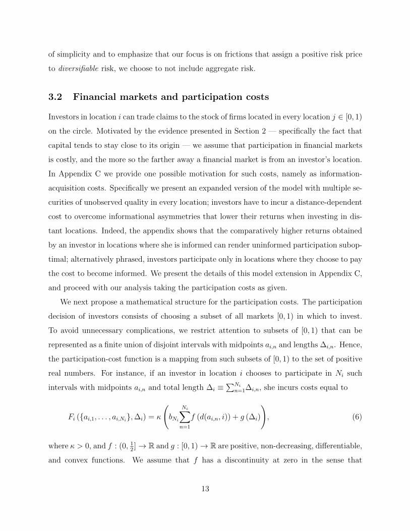
We next propose a mathematical structure for the participation costs. The participation

decision of investors consists of choosing a subset of all markets [0, 1) in which to invest.

To avoid unnecessary complications, we restrict attention to subsets of [0, 1) that can be

represented as a finite union of disjoint intervals with midpoints ai,n and lengths ∆i,n. Hence,

the participation-cost function is a mapping from such subsets of [0, 1) to the set of positive

real numbers. For instance, if an investor in location i chooses to participate in Ni such

intervals with midpoints ai,n and total length ∆i ≡∑Ni

n=1∆i,n, she incurs costs equal to

Fi ({ai,1, . . . , ai,Ni},∆i) = κ

(bNi

Ni∑n=1

f (d(ai,n, i)) + g (∆i)

), (6)

where κ > 0, and f : (0, 12]→ R and g : [0, 1)→ R are positive, non-decreasing, differentiable,

and convex functions. We assume that f has a discontinuity at zero in the sense that

13

!"!" !"

Figure 4: Illustration of participation choices under different assumptions on the participationcosts Fi ({ai,1; ..; ai,Ni},∆i).

limx→0 f (x) > 0, while f(0) = 0. Also, g(0) = 0 and g′(0) = 0. Finally, bNi is positive and

non-decreasing in Ni; we set b1 = b2 = 1 without loss of generality.10

We make several remarks on specification (6). First we note that Fi ({i}, 0) = 0, so that

participating only in the local market is costless. Second, the fact that f is increasing implies

that investing in markets that are farther away (in the sense that the distance d(ai,n, i) from

one’s location is larger) is more costly than participating in markets that are close by. Third,

increasing the total mass of markets in which the investor participates (∆i), while keeping

the number (and midpoints) of intervals the same, incurs incremental rather than fixed costs.

This captures the idea that expanding participation to contiguous markets is substantially

less costly than participating in a market that is not adjacent to any of the markets where the

investor has already decided to participate. Fourth, the fact that participation costs depend

on the location of the investor implies that investors in different locations on the circle face

different costs of participating in a given market j, depending on their proximity to that

market. Finally, for technical convenience and ease of exposition, the costs of expanding the

total measure of the interval are specified as independent of the structure of the midpoints

and the lengths of the subintervals. This assumption is not crucial and can be easily relaxed.11

Even though one can specify more elaborate participation-cost structures, the one given

by (6) is sufficiently flexible for our purposes. To better understand this cost structure

it is useful to consider some special cases. In the first special case, the investor can only

10Since f(0) = 0, the first mid-point that an investor chooses is always her home location. Hence b1 can bechosen arbitrarily, as b1f(0) = 0. Similarly, b2 = 1 is without loss of generality, since we can always re-definef∗ = b2f and b∗N = bN

b2without changing the total cost Fi.

11Indeed, if one were to replace g(∆i) with∑Ni

n=1 g (∆i,n), that would introduce additional reasons for thecost structure to be non-convex, strengthening some of the conclusions of the paper.

14

participate in an arc centered at her home location (depicted in the left plot of Figure 4).

This outcome follows from (6) if one sets bNf (x) = ∞ and g(y) < ∞ for any x > 0,

y > 0, and N > 1, so that the participation cost reduces to F (∆i) = κg(∆i). We note

that in this special case the participation-cost structure is convex (unlike when the investor

participates in disjoint intervals, which carries fixed costs). This convexity is quite attractive

for illustrating some of the results of the paper, and therefore this special case will play an

important role in our analysis. A second special case corresponds to situations in which an

investor only participates on discrete points (middle plot of Figure 4). This outcome obtains

from (6) if bNf (x) <∞ and g(y) =∞ for any y > 0. In the general case bNf (x) <∞ and

g (y) <∞, the participation decision involves choosing the number of points Ni, the location

of the midpoints ai,n, and the length of the intervals ∆i,n at each location. This situation is

depicted in the right plot of Figure 4.

Besides the markets for risky shares, there is a market for zero-net-supply riskless bonds

that pay one unit of wealth at time 1. Participation in the bond market is costless for

everyone.

The participation costs act as deadweight costs that are paid out (i.e., reduce consump-

tion) at time 1.

We remark in passing that our results would not be affected if, instead of making the

participation decisions themselves, agents invested through frictionless and competitive in-

termediation. That is, we could introduce a competitive sector of intermediaries who incur

the participation costs, choose optimal portfolios for their clients, and then charge them

competitive fees to cover the participation costs.12

12In a previous version of the paper, we consider such a model. Specifically, in this model a) investorsdon’t have direct access to markets, but rather have to hire (competitive) intermediaries in their locationto gain access to distant markets, b) the intermediaries attract clients by offering portfolios that maximizetheir welfare, and c) intermediaries charge clients fees to cover the participation costs that they incur. Notsurprisingly, the assumption of perfect competition and the lack of frictions between investors and interme-diaries (no moral hazard, unobservable, idiosyncratic liquidity shocks. etc.) implies that the allocations andthe prices in the two models are identical.

15

3.3 Individual maximization and equilibrium

To formalize an investor’s decision problem we let Pi denote the price of a share in a market

i, PB ≡ 11+r

the price of a bond, dX(i)j the mass of shares in market j bought by an investor

located in i,13 and X(i)B the respective number of bonds. Then, letting

W0,i ≡∫ 1

0

PjdX(i)j + PBX

(i)B

denote the total financial wealth of an investor in location i, the budget constraint of an

investor can be expressed as W0,i = Pi.

We are now in a position to formulate the investor’s maximization problem as

maxwfi ,G

(i),Ni,−→a i,−→∆i

E [U (W1,i)] , (7)

subject to the budget constraint W0,i = Pi, and

W1,i = W0,i

(wfi (1 + r) +

(1− wfi

)∫ 1

0

RjdG(i)j

)− Fi, (8)

where wfi is the fraction of W0,i invested in the risk-free security by an agent in location i,

G(i)j is a bounded-variation function with

∫ 1

0dG

(i)j = 1, which is constant in locations where

the investor does not participate (i.e., dG(i)j =0 in these locations), so that dG

(i)j captures the

fraction of the risky component of the portfolio(

1− wfi)W0,i invested in the share of stock

j by a consumer located in i. Finally, Ri ≡ DiPi

is the realized gross return on security i at

time 1. We do not restrict G to be continuous, that is, we allow investors to invest mass

points of wealth in some locations.

The definition of equilibrium is standard. An equilibrium is a set of prices Pi, a real inter-

est rate r, and participation and portfolio decisions wfi , G(i), Ni, and {ai,1, . . . , ai,Ni ,∆i,1, . . . ,∆i,Ni}

for all i ∈ [0, 1] such that: 1) wfi , G(i), Ni, and {ai,1...ai,Ni ,∆i,1...∆i,Ni} solve the optimization

problem of equation (7), 2) financial markets for all stocks clear: Pj =∫i∈[0,1]

(1− wfi

)W0,idG

(i)j ,

13The function X(i)j has finite variation. We adopt the natural convention that X

(i)j is continuous from

the right and has left limits.

16

and 3) the bond market clears, i.e.,∫i∈[0,1]

W0,iwfi di = 0.

By Walras’ law, we need to normalize the price in one market. Since in the baseline

model we abstract from consumption at time zero for parsimony, we normalize the price of

the bond to be unity (i.e., we choose r = 0). We discuss consumption at more dates than

time one and an endogenously determined interest rate in Appendix A.1.

4 Solution and Its Properties

We solve the model and illustrate its properties in a sequence of steps. First, we discuss a

frictionless benchmark, where participation costs are absent. Second, in order to highlight

the core intuition, we discuss the special case where the investor can only participate in

an arc centered at her location, so that her participation decision amounts to choosing the

length of that arc (the special case depicted on the left panel of Figure 4). We consider the

general case, which allows for both contiguous and non-contiguous participation choices, in

Appendix A.2.

4.1 A frictionless benchmark

As a benchmark, we consider first the case without participation costs: Fi = 0. In this case,

the solution to the model is trivial. Every investor i participates in every market j. The first

order condition for portfolio choice is

E [U ′(W1,i) (Rj − (1 + r))] = 0. (9)

With the above first-order condition in hand, one can verify the validity of the following

(symmetric) equilibrium: wfi = 0, and G(i)j = Gj = j for all (i, j) ∈ [0, 1) × [0, 1) — i.e.,

investors in all locations i choose an equally weighted portfolio of every share j ∈ [0, 1].

Accordingly, W1,i =∫ 1

0Djdj = 1. Since in this equilibrium W1,i = 1, the Euler equation (9)

implies that

E(Rj) = 1 + r. (10)

17

Combining (10) with the definition Rj =DjPj

implies

Pj =E (Dj)

1 + r=

1

1 + r= 1, (11)

where the last equation follows from the normalization r = 0.

The equilibrium in the frictionless case is intuitive. Since there are no participation costs,

investors hold an equally weighted portfolio across all locations. Since — by assumption —

there is no risk in the aggregate, the risk of any individual security is not priced.

4.2 Symmetric equilibria with participation costs

To facilitate the presentation of some of the key results, we focus on the special case depicted

in the left plot of Figure 4, i.e., the case where the investor’s participation choice amounts

to choosing the length ∆ of an arc centered at her location. The associated participation

cost is κg(∆).

To make the investor’s problem well-defined and interesting, we assume that the costs of

participation increase sufficiently fast (and thus become infinite) as ∆ approaches one:

Assumption 1 lim∆→1 g′ (∆) (1−∆)4 =∞.

Assumption 1 helps ensure that an optimal ∆ less than one exists for every investor.14

Before presenting results, we introduce a convention to simplify notation.

Convention 1 For any real number x, let bxc denote the floor of x, i.e., the largest integer

weakly smaller than x. We henceforth use the term “location x” (on the circle) to refer to

the unique point in [0, 1) given by xmod 1 ≡ x− bxc.

With this convention we can map any real number to a unique location on the circle with

circumference one. For example, this convention implies that the real numbers -0.8, 0.2,

14If P < 1, so that there is a risk premium, the limiting case ∆ = 1 is not well defined, since both thecosts and the benefits of participation diverge to infinity as ∆→ 1. Assumption 1 along with an applicationof L’Hopital’s rule ensures that the cost component dominates the benefit component as ∆→ 1, resulting inan optimal (interior) choice of ∆ ∈ [0, 1). We also note that, if we introduce aggregate risk, then Assumption1 can be replaced with the weaker lim∆→1 g (∆) = ∞. Finally, no assumption is necessary in the presenceof a leverage constraint, as in Section 5 (except that g(∆) > 0 for some ∆ ∈ (0, 1)).

18

and 1.2 correspond to the same location on the circle with circumference one, namely 0.2.

An implication of this convention is that any function h defined on the circle extends to a

function h on the real line that is periodic with period one, i.e., h(x) = h(x + 1) = h(x

mod 1). From now on, we treat functions on the circle also as functions defined on the entire

real line.

We next introduce two definitions.

Definition 1 The standardized portfolio associated with G(i)j is the function L : R → [0, 1]

defined by Lj = G(i)i+j.

The notion of a standardized portfolio allows us to compare portfolios of investors at

different locations on the circle. For example, if all investors choose portfolios with weights

that only depend on the distance d between their domicile and the location of investment,

and these distance-dependent weights are the same for all investors, then these investors

hold the same standardized portfolio.

Definition 2 A symmetric equilibrium is an equilibrium in which all agents choose the same

participation interval ∆, the same leverage wf , and the same standardized portfolio.

Due to the symmetry of the problem, it is natural to start by attempting to construct a

symmetric equilibrium.

Proposition 1 For any ∆ ∈ (0, 1) define

L∗j ≡

0 if j ∈ [−1

2,−∆

2)

j + 12

if j ∈ [−∆2, ∆

2)

1 if j ∈ [∆2, 1

2)

(12)

and

ω (∆) ≡ V ar

(∫ 1

0

Dj dL∗j

)=σ2

12(1−∆)3 . (13)

19

Finally, let ∆∗ denote the (unique) solution to the equation

κg′ (∆∗) = −γ2ω′ (∆∗) (14)

and also consider the set of prices

Pi = P ≡ 1− γω (∆∗) . (15)

Then, assuming that a symmetric equilibrium exists, the choices ∆(i) = ∆∗, wfi = 0, dG(i)j =

dL∗j−i, and prices Pi = P constitute the unique symmetric equilibrium.

Proposition 1 gives simple, explicit expressions for both the optimal portfolios and par-

ticipation intervals. To understand how these quantities are derived, we take an individual

agent’s wealth W1,i from (8) and we assume that prices for risky assets are the same in all

locations. Then, using W0,i = Pi = P , r = 0, Rj =DjP, and Fi = κg (∆) , we express W1,i as

W1,i = P

(wfi +

(1− wfi

)∫ 1

0

RjdG(i)j

)− κg (∆)

=

(Pwfi +

(1− wfi

)∫ 1

0

DjdG(i)j

)− κg (∆) .

Because of exponential utilities and normally distributed returns, maximizing EU (W1,i) is

equivalent to solving

maxdG

(i)j ,∆,wfi

Pwfi +(

1− wfi)∫ 1

0

EDjdG(i)j −

γ

2

(1− wfi

)2

V ar

(∫ 1

0

DjdG(i)j

)−κg (∆) . (16)

Noting that EDj = 1, inspection of equation (16) shows that (for any wf and ∆) the opti-

mal portfolio is the one that minimizes the variance of dividends in the participation interval

∆. Since the covariance matrix of dividends is location invariant, the standardized variance-

minimizing portfolio is the same at all locations. Solving for this variance-minimizing port-

folio Lj is an infinite-dimensional optimization problem. However, because of the symmetry

of the setup we are able to solve it explicitly, and equation (12) provides the solution. The

optimal portfolio, L∗j , corresponds to the distribution that minimizes the sum of the vertical

20

distances to the uniform distribution on[−1

2, 1

2

), subject to the constraints that Lj = 0 for

j ∈ [−12,−∆

2) and Lj = 1 if j ∈ [∆

2, 1

2). The resulting optimized variance is given by ω (∆),

defined in (13).

Accordingly, the agent’s problem can be written more compactly as

V = max∆,wfi

Pwfi +(

1− wfi)− γ

2

(1− wfi

)2

ω (∆)− κg (∆) . (17)

The first-order conditions with respect to wfi , respectively ∆, are

1− P = γ(

1− wfi)ω (∆) (18)

κg′ (∆) = −γ2

(1− wfi

)2

ω′ (∆) . (19)

Since in a symmetric equilibrium market clearing requires wfi = 0, equation (18) becomes

identical to (15) and (19) becomes equivalent to (14).

Equation (14) makes explicit the resolution of the tradeoff between participation costs

and risk taking. Specifically, the participation interval is determined as the point where

the marginal cost of participation, κg′ (∆), is equal to the marginal benefit of participation,

−γ2ω′ (∆).

Figure 5 illustrates this tradeoff by plotting the marginal cost from increasing ∆, namely

κg′ (∆), against the respective marginal benefit −γ2ω′ (∆) . Since g(∆) is convex, g′(∆) is up-

ward sloping. By contrast, the marginal benefit is declining, since −ω′′(∆) = −σ2

2(1−∆) <

0. Since g′ (0) = 0, lim∆→1 g′ (∆) =∞, −ω′ (0) > 0, and ω′ (1) = 0, the two curves intersect

at a unique point ∆∗ ∈ [0, 1).

Proposition 1 helps capture the economic mechanisms that underlie our model. Consider,

for instance, its implications for a reduction in the cost of accessing markets (i.e., a reduction

in κ). As Figure 5 illustrates, such a reduction increases the degree of participation ∆ and

promotes portfolio flows across different locations. In turn, this increased participation im-

proves risk sharing across different locations, which leads to higher prices of risky securities,

P = 1− γω (∆), and accordingly lower risk premia. By contrast, an increase in the costs of

accessing risky markets leads to a lower ∆ and a higher degree of concentration of risk. The

21

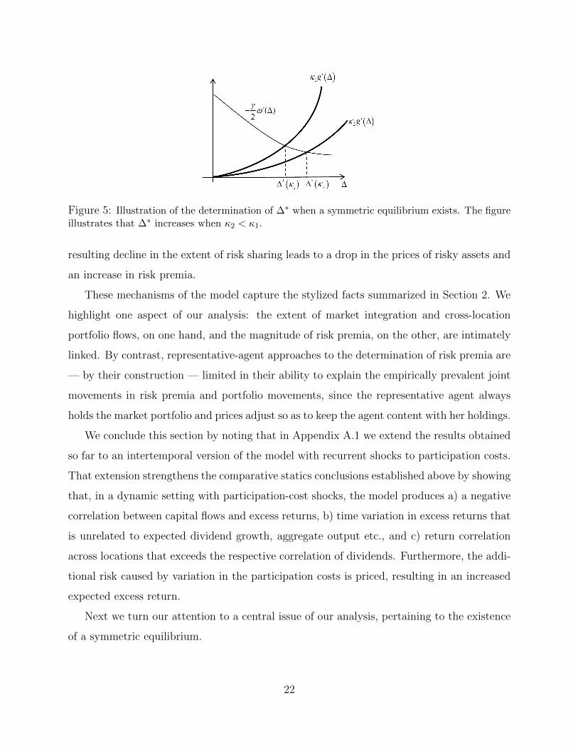
Figure 5: Illustration of the determination of ∆∗ when a symmetric equilibrium exists. The figureillustrates that ∆∗ increases when κ2 < κ1.

resulting decline in the extent of risk sharing leads to a drop in the prices of risky assets and

an increase in risk premia.

These mechanisms of the model capture the stylized facts summarized in Section 2. We

highlight one aspect of our analysis: the extent of market integration and cross-location

portfolio flows, on one hand, and the magnitude of risk premia, on the other, are intimately

linked. By contrast, representative-agent approaches to the determination of risk premia are

— by their construction — limited in their ability to explain the empirically prevalent joint

movements in risk premia and portfolio movements, since the representative agent always

holds the market portfolio and prices adjust so as to keep the agent content with her holdings.

We conclude this section by noting that in Appendix A.1 we extend the results obtained

so far to an intertemporal version of the model with recurrent shocks to participation costs.

That extension strengthens the comparative statics conclusions established above by showing

that, in a dynamic setting with participation-cost shocks, the model produces a) a negative

correlation between capital flows and excess returns, b) time variation in excess returns that

is unrelated to expected dividend growth, aggregate output etc., and c) return correlation

across locations that exceeds the respective correlation of dividends. Furthermore, the addi-

tional risk caused by variation in the participation costs is priced, resulting in an increased

expected excess return.

Next we turn our attention to a central issue of our analysis, pertaining to the existence

of a symmetric equilibrium.

22

4.3 Asymmetric, location-invariant equilibria: Leverage and the

diversity of financial strategies

Proposition 1 contains the premise that a symmetric equilibrium exists. Surprisingly, despite

the symmetry of the model setup, a symmetric equilibrium may fail to exist. Instead, the

market equilibrium may involve different choices (leverage ratios, portfolios of risky assets,

wealth allocations, etc.) for agents in the same location, even though these agents have

the same preferences and endowments and are allowed to make the same participation and

portfolio choices.

These claims are explained by the observation that the necessary first-order conditions

resulting in the prices Pi = P = 1−γω (∆∗) are not generally sufficient. We now take a closer

look at whether a symmetric equilibrium exists. Specifically, we fix the price P = 1−γω (∆∗)

of Proposition 1 and investigate whether (and under what conditions) the choices wf = 0

and ∆ = ∆∗ are indeed optimal for the investor.

To answer this question, we consider again the maximization problem (17). Taking

P = 1 − γω (∆∗) as given, substituting into (18), and re-arranging implies that if investors

allocate their wealth over a participation interval ∆ (potentially different from ∆∗), then

1− wf =ω (∆∗)

ω (∆). (20)

Equation (20) contains an intuitive prediction. An investor allocating her wealth over a

span ∆ > ∆∗ is facing the same average returns, but a lower variance ω (∆), and hence a

higher Sharpe ratio compared to an investor allocating her wealth over an interval of size ∆∗.

Accordingly, the former investor finds it optimal to leverage her portfolio. This is reflected

in equation (20), which states that wf < 0(wf > 0

)whenever ∆∗ < ∆ (∆∗ > ∆) .

An interesting implication of (19) is that the marginal benefit of an increased participation

interval becomes larger with leverage. This is intuitive since increased leverage implies a more

volatile wealth next period and hence a higher marginal benefit of reducing that variance by

increasing ∆. In short, the choices of ∆ and of leverage 1− wf are complements.

This complementarity can lead to an upward sloping marginal benefit of increased par-

23

   

   

Δ* ΔΔ*2

κg ' Δ( )

−γ2ω '(Δ)

Δ* Δ

κg ' Δ( )

−γ2ω '(Δ)

−γ2(1−w f (Δ;Δ*))2ω '(Δ)

Δ1*

−γ2(1−w f (Δ;Δ* ))2ω '(Δ)

Figure 6: Illustration of the marginal benefit curve −γ2

(ω(∆∗)ω(∆)

)2ω′ (∆) , the marginal cost curve

κg′ (∆) and the marginal benefit curve −γ2ω′ (∆) restricting wf = 0. The left plot illustrates a case

where a symmetric equilibrium exists whereas the right plot illustrates a case where a symmetricequilibrium fails to exist.

ticipation. Indeed, with our cash-flow specification, substituting (20) into (19) gives

κg′ (∆) = −γ2

(ω (∆∗)

ω (∆)

)2

ω′ (∆) . (21)

Using the fact ω (∆) = σ2

12(1−∆)3, the right hand side can be expressed as−γ

2

(ω(∆∗)ω(∆)

)2

ω′ (∆) =

γσ2

8(1−∆∗)6 (1−∆)−4 , which is increasing in ∆.

Figure 6 helps illustrate these notions. The figure depicts the marginal cost curve κg′ (∆),

the marginal benefit curve −γ2

(1− wf (∆; ∆∗)

)2ω′ (∆) = −γ

2

(ω(∆∗)ω(∆)

)2

ω′ (∆), and also the

curve −γ2ω′ (∆) , i.e., the marginal benefit of participation fixing wf = 0. The point where all

three curves intersect corresponds to the point ∆ = ∆∗. The left plot of Figure 6 illustrates

a case where a symmetric equilibrium exists, whereas the right plot illustrates a case where

a symmetric equilibrium fails to exist. The difference between the two plots is the shape of

g′ (∆). In the left plot g′ (∆) intersects the marginal benefit curve only once, namely at ∆∗.

For values smaller than ∆∗, the marginal benefit of participation is above the marginal cost

and vice versa for values larger than ∆∗. Hence, in this case ∆∗ is indeed the optimal choice

for the investor.

This is no longer the case in the right plot. Here the marginal benefit curve intersects the

marginal cost curve three times (at ∆∗1, ∆∗, and ∆∗2). Since the marginal benefit is below the

24

   

   

ΔΔ**2Δ**1

κg ' Δ( )

l P2( )

l P3( )

l P1( )

Figure 7: Illustration of an asymmetric equilibrium involving mixed strategies. The price adjustsso that area A is equal to area B. Accordingly, an investor is indifferent between ∆∗∗1 and ∆∗∗2 .Here, P3 < P2 < P1 < 1.

marginal cost for values of ∆ that are smaller and “close” to ∆∗, while the marginal benefit

is larger than the marginal cost for values of ∆ that are larger and “close” to ∆∗, ∆∗ is a

local minimum, and hence a suboptimal choice. By contrast the points ∆∗1 and ∆∗2 are local

maxima. (In this particular example the point ∆∗1 is the global maximum, since the area A

is larger than the area B.) The fact that ∆∗ is not a maximum implies that there does not

exist a symmetric equilibrium, since in a symmetric equilibrium it would have to be the case

that wf = 0.

The non-existence of a symmetric market equilibrium implies that one should look for

equilibria where investors in the same location make different choices, even though they have

the same preferences, endowments, and information. Figure 7 presents a simple graphical

illustration of such an equilibrium in the context of the example depicted on the right plot

of Figure 6.

Specifically we illustrate the construction of an equilibrium that features the same price

Pi = P for all markets, but where a fraction π of investors in every location i choose

(wf1 ,∆1), while the remaining fraction (1 − π) of agents choose (wf2 ,∆2). We refer to such

an equilibrium as an asymmetric, location-invariant equilibrium. We introduce a function l

25

that captures the marginal benefit of participation as a function of ∆ and P :

l (∆, P ) ≡ −γ2

(1− wf (∆, P )

)2ω′ (∆) = −γ

2

(1− Pγ

)2ω′ (∆)

ω2 (∆), (22)

where the last equation follows from (18).

Figure 7 depicts the function l (∆, P ) for three values P1 < P2 < P3 < 1. A first

observation is that as P declines from P3 to P1, the curve l (∆, P ) shifts up. Moreover

there exists a level P2 and associated values ∆∗∗1 and ∆∗∗2 for which the area “A” equals

the area “B”, so that investors are indifferent between choosing ∆∗∗1 and ∆∗∗2 . Fixing these

values of P,∆∗∗1 , and ∆∗∗2 , we can determine the values of wf1 and wf2 from (18). As part

of the proof of Proposition 2 (in the appendix), we show that these values of wf1 and wf2

satisfy 1 − wf1 < 1 < 1 − wf2 . In order to clear the bond market, π has to be so that

πwf1 + (1− π)wf2 = 0, i.e., π =wf2

wf2−wf1

∈ (0, 1).15 We also show in the appendix that for this

value of π all markets for risky assets clear as well.

The next proposition generalizes the insights of the above illustrative example. It states

the existence of an asymmetric, location-invariant equilibrium when a symmetric equilibrium

fails to exist.

Proposition 2 When the cost function g is such that a symmetric equilibrium fails to exist,

there exists an asymmetric, location-invariant equilibrium. Specifically, there exist (at least)

two tuples{

∆k, wfk

}, k ≥ 2, and πk > 0 with

∑kπk = 1 and

∑kπk(1 − wfk

)= 1, such

that in every location i a fraction πk of agents choose the interval, leverage, and portfolio

combination{

∆k, wfk , dL

(k)}, where dL(k) is the measure given in (12) for ∆ = ∆k. The

price of risky assets is uniquely determined in the class of location-invariant equilibria,16

and in particular a symmetric and an asymmetric location-invariant equilibrium involving

different prices cannot co-exist.

The model can therefore generate situations in which a symmetric equilibrium can fail to

15It holds that π ∈ (0, 1) because wf2 < 0 and wf1 > 0.16It is possible, for special parameter constellations, that in an asymmetric equilibrium an investor is

indifferent between multiple (not just two) tuples of participation and leverage combinations. Accordingly,for the same price one could construct asymmetric equilibria with different combinations of asymmetricstrategies. However — by construction — any two such equilibria would feature the same price for all assets.In this sense an asymmetric equilibrium is essentially unique.

26

exist. Instead, the market equilibrium features a diverse set of financial strategies, with some

investors pursuing high-cost, high-Sharpe-ratio, high-leverage strategies and some investors

pursuing low-cost, low-Sharpe-ratio, no-leverage strategies. The first type of strategies is

akin to the sort of strategies offered by hedge funds, while the second type of strategies is

akin to those offered by mutual funds.

A novel feature of our model is that it helps isolate a source of non-concavity of the

participation decision that is distinct from non-convex participation-cost structures. Specif-

ically, the continuity of the dividend structure in our framework along with the convexity of

g(∆) allow us to model the participation choice (i.e., the choice of ∆) as a concave decision

problem for fixed leverage. Accordingly, we can illustrate the role of the complementarity

between leverage and participation in rendering the participation problem non-concave. The

distinct role of this complementarity can be easily overlooked in models with discrete mar-

kets where the participation choice itself (i.e., even with fixed leverage) is discrete and hence

necessarily non-convex.

Clearly, if we were to introduce elements of non-convexity into the cost structure (for

instance, because investors may choose non-contiguous participation locations, as in the next

section or in Appendix A.2), there is an additional and conceptually distinct reason why the

investor’s objective is non-concave, leading to the adoption of diverse financial strategies.17

In summary, this section has established that the non-concavities in investors’ objective

functions introduce diversity in the optimal participation-leverage combinations chosen by

different investors. Importantly, the equilibrium price plays a key role in determining the

participation-leverage combinations that keep investors indifferent between different strate-

gies. In the next section we identify a tension that arises when we introduce collateral con-

straints, so that the price simultaneously affects investors’ indifference relations and their

feasible leverage-participation combinations.

17A classic example, which also features different choices by ex-ante identical investors, due to fixed (hencenon-convex) information costs, is Grossman and Stiglitz (1980). A difference between Grossman and Stiglitz(1980) and our setup, which becomes pertinent in the next section, is that the price adjusts to keep investorsindifferent between different combinations of leverage and participation, while in Grossman and Stiglitz(1980) investors decide on paying information acquisition costs before observing the price.

27

5 Collateral Constraints and the Complementarity be-

tween Leverage and Participation

The previous section shows that equilibrium outcomes may feature heterogeneous investment

strategies in every location despite the fact that investors are identical. An important aspect

of these heterogeneous strategies is that they require different degrees of leverage. Even

though in the model leverage can be chosen freely, in reality leverage is limited by collateral

constraints. In this section we discuss the implications of such constraints. We present a

simple example to show that leverage constraints open the possibility for multiple location-

invariant equilibria. Accordingly, prices, capital flows, and leverage exhibit discontinuous

dependence on changes to participation costs.

To model collateral constraints, we let χ ∈ [0, 1) denote a “haircut” parameter and require

[(1− χ)

∫ 1

0

PjdX(i)j − Fi

]+X

(i)B ≥ 0. (23)

Equation (23) stipulates that the borrowing capacity of an investor (the first term — inside

the square brackets — of (23)) do not exceed the amount the investor actually borrows (the

second term of (23)). The investor’s borrowing capacity is computed as the market value of

the collateral net of the haircut and of the obligation the investor has already assumed by

committing to pay the participation costs in period 1.

The collateral constraint (23) is pervasive in reality, extensively used in the literature,

and analytically convenient for our purposes. Therefore, we focus on the implications of this

constraint in the body of the paper. In Appendix D we analyze an alternative, endogenous

version of the constraint (23) motivated by the desire to prevent default in all states of

nature. We show that the key findings of the present section remain the same.

To further streamline the exposition, we choose a particularly simple specification for the

participation-cost structure that includes a discrete element of participation choice. This

choice introduces an additional and direct reason for the existence of asymmetric equilibria

featuring heterogenous leverage. More importantly, it allows us to provide an analytically

solvable example of participation and leverage choice that helps illustrate the role of leverage

28

constraints when these two choices interact.

Specifically, we postulate the cost function depicted in the middle graph of Figure 4. In

that case, the optimal participation choice amounts to choosing the location of the points

ai and the number of the discrete points N .18 To keep computations as simple as possible,

we assume furthermore that bN = ∞ for N > 2, so that only choices involving N ≤ 2 are

feasible.19 Accordingly, an investor’s problem comes down to choosing N = 1 (and paying

no participation costs) or N = 2 and the distance d from her home location, resulting in

participation costs equal to κf(d). (See Appendix A.2 for an extension to multiple locations.)

In an effort to further streamline the analysis, we assume that f ′(d) = 0. In that case the

investor faces only a fixed cost of κf0 when choosing N = 2, but can choose d freely (i.e.,

without incurring additional cost).

We start by analyzing equilibrium prices in this economy when we don’t impose the

constraint (23) on investors’ decisions.

Proposition 3 Assume that the borrowing constraint is not imposed on investors’ decisions,

and also assume that κ ∈ (κ1, κ2), where κ1 ≡ 1128

γσ2

f0, κ2 ≡ 1

8γσ2

f0. Then there exists a unique

asymmetric equilibrium in which a fraction π > 0 of the investors choose N = 1, while the

rest choose N = 2 and d = 12. The equilibrium price in all locations is

P (κ) = 1− σ√γκf0

18, (24)

and the choices wfi satisfy wf1 > 0 and wf2 < 0.

For values of κ smaller than κ1 or larger than κ2 the equilibrium is symmetric (and unique

in the class of location-invariant equilibria) with everyone choosing N = 2 and d = 12

or

everyone choosing N = 1, respectively. Hence, without imposing the constraint (23), the left

plot of Figure 8 gives a visual depiction of P (κ), which is a continuous function of κ.

18Recall that in this case there is a minimum “fixed” cost that one needs to pay for every new locationthat she chooses given by κbN limx→0 f(x) > 0.

19The condition bN = ∞ can be substantially weakened. Indeed all that is needed for N = 1 or N = 2to be the only feasible choices is that κbN limx→0 f(x) > 1 for N > 2. To see this, use the normalization

PB = 1 along with the budget constraint to obtain Pi = W0,i =∫ 1

0PjdX

(i)j + X

(i)B = (1 − χ)

∫ 1

0PjdX

(i)j −

Fi+X(i)B +Fi+χ

∫ 1

0PjdX

(i)j ≥ Fi+χ

∫ 1

0PjdX

(i)j , where the inequality follows from (23). Noting that Pj ≤ 1

and f is non-decreasing, the only feasible choices are N = 1 or N = 2 if κbN limx→0 f(x) > 1 for N > 2.

29

0 1 2 3 4 5 6 70.55

0.6

0.65

0.7

0.75

0.8

0.85

0.9

0.95

g

P(g)

0 1 2 3 4 5 6 70.55

0.6

0.65

0.7

0.75

0.8

0.85

0.9

g

P(g)

g1 g2gc

Locus of pointswhere theconstraint justbinds

Price ignoring the constraint

Actual Price

Figure 8: The left plot depicts the price P (κ) assuming the leverage constraint is not binding.

The downward-sloping dotted line on the right plot plots the same quantity, along with the actual

price (solid line) and the locus of points such that the leverage constraint is just binding (upward

sloping line). Hence for points above and to the left of the upward sloping line the constraint is not

binding, whereas it is binding for points below and to the right. Parameters used in this example:

γ = 5, f0 = 0.1, χ = 0.2, σ = 1.

When imposing the constraint (23), however, a different situation arises: For any given

value of κ there may be multiple equilibria. A direct implication of equilibrium multiplicity

is that it may become impossible to find a continuous mapping κ 7→ P (κ). Such a situation

is depicted in the right plot of Figure 8, which graphs the equilibrium price in the absence

of constraints, the locus of points where the constraint is binding, and the maximum price

associated with an equilibrium when the constraint is binding.

To understand the source of multiple equilibria and why they imply the non-existence of

a continuous mapping κ → P (κ), it is useful to refer to Figure 9. For each subplot we fix

a value of κ. Given that value of κ, the line denoted “Indifference” in each subplot depicts

combinations of P and possible choices of (1−wf2 ) such that the indifference relation V1 = V2

holds.20 Similarly, the line denoted “Constraint” depicts combinations of P and 1−wf2 such

that the constraint (23) binds with equality, i.e., the set of points such that21

κf0 = P(

1− χ(1− wf2 )). (25)

20See equation (47) in the appendix for a formal statement of the indifference relation.21Combining the investor’s budget constraint with (23) and repeating the same steps as in footnote 19

gives W0,i ≥ Fi + χ∫ 1

0PjdX

(i)j . Evaluating this inequality with Pi = Pj = P = W0,i, PB = 1, Fi = κf0, and∫ 1

0dX

(i)j = 1− wfi gives (25).

30

Accordingly, all the points that lie above that line are admissible combinations of P and

1 − wf2 . The line denoted “FOC” (in the first plot) depicts the combination of points that

satisfy the (unconstrained) first-order condition for leverage

1− P = γ(

1− wf2)ω(N=2),

where ω(N=2) = σ2

48is the minimal variance attainable for an investor choosing to participate

in N = 2 locations. Finally, the line denoted “Lowest Price” is a reference line denoting

the price that would obtain in the symmetric equilibrium where all investors participate

exclusively in their own location.

The left plot depicts the case κ = κc. In that case the three lines “FOC”, “Indifference”,

and “Constraint” intersect at the same point (C). This reflects that when κ = κc, the

equilibrium combination of price and the (unconstrained) optimal leverage for an investor

choosing N = 2 are such that the constraint just binds. Moreover, point C is the unique

equilibrium.

For (moderately) higher values of κ, illustrated in the middle panel, the constraint binds

actively, so that the first order condition for the optimal choice of leverage no longer holds

with equality. Instead, candidate asymmetric equilibria are given by the intersection of

“Indifference” and “Constraint”. Clearly, there are two such equlibria (points C′ and D′).

The symmetric equilibrium whereby everyone chooses N = 1 is yet another equilibrium. (To

see this, note that point A′ is to the right of point B′. This implies that if all investors

choose N = 1 and zero leverage, then an individual investor would not benefit by deviating

to N = 2; if she did deviate, her leverage would be given by the point B′, which is above

and to the left of the line labeled “Indifference” — hence inferior to choosing N = 1).

The right-most plot shows a case in which κ is large enough that there is no point of

intersection between the lines “Indifference” and “Constraint”. At that point there can be

no asymmetric equilibria. The equilibrium becomes symmetric, i.e., the price drops to the

level that obtains when everyone chooses N = 1 and wf = 0.

The multiplicity of equilibria implies that the mapping κ 7→ P (κ) is discontinuous at

31

1 1.5 2 2.5 30.4

0.45

0.5

0.55

0.6

0.65

0.7

0.75

0.8

0.85

0.9

1−wf

Pκ= 3.092

1.7 1.8 1.9 2 2.1

0.57

0.58

0.59

0.6

0.61

0.62

0.63

1−wf

P

κ= 3.7413

1.7 1.8 1.9 2 2.10.55

0.56

0.57

0.58

0.59

0.6

0.61

0.62

0.63

0.64

0.65

1−wf

P

κ= 3.7722

FOC

Indifference

C’

C

A B

Constraint

D’

Indifference

Constraint

Indifference

Constraint

Lowest Price

A’ A’’B’

B’’

Lowest Price

Lowest Price

Figure 9: For three different values of the cost parameter κ, the three plots depict combinations

of price (P ) and leverage (1 − wf2 ) so that (i) investors are indifferent between adopting no- and

high-leverage strategies (line labeled “Indiference”); (ii) investors’ choices of leverage (1− wf2 ) are

(unconstrained) optimal given P (line labeled “FOC”); and (iii) the leverage constraint just binds

(line labeled “Constraint”). For reference, we also plot the equilibrium price associated with all

investors participating exclusively in their own location (line labeled “Lowest price”). Parameters

are identical to Figure 8.

some value κ > κc, no matter how one selects the equilibrium. 22 This outcome, albeit in a

different context, is reminiscent of Gennotte and Leland (1990).

To understand intuitively why multiple equilibria arise when the leverage constraint is

binding, it is useful to start with the case when the constraint is not binding. In that case

the incentives to pursue broad-participation strategies are substitutes across investors: The

less other investors choose to participate in such strategies, the lower the prices of risky

assets, and thus the higher an individual investor’s incentive to pursue such strategies. As is

commonly the case when economic decisions are substitutes, the equilibrium is unique and

features a price that keeps investors indifferent between broad- and narrow-participation

strategies.

A different situation arises when the leverage constraint binds. Reductions in prices

increase the Sharpe ratio of risky strategies, but also reduce the ability to leverage. Since

22For instance if one chooses the equilibrium associated with the maximal price, then the discontinuitywill occur for some value of κ between those depicted in the middle and the right-most panel of Figure 9.Similarly, if one chooses the equilibrium with the minimal price, then the jump will occur at some value of κbetween those depicted in the left-most and middle graph. More generally, it is impossible to find a choice ofequilibrium such that P (κ) is continuous for the values of κ between the left-most and the right-most plots.

32

leverage and participation choices are complements, a decline in price may end up lowering,

rather than increasing, the incentive to participate, rendering the choices to pursue broad-

participation strategies complements across investors, rather than substitutes. As a result,

there can be multiple equilibria: If prices are low, then leverage is constrained to be low

and there isn’t enough incentive to participate broadly, justifying low prices. If prices are

high, then agents can leverage sufficiently to justify paying for broad participation, which

supports high prices. Note that the cost κ can’t be either too high or too low for these

different equilibria to obtain. Fragility is an immediate consequence of the existence of

multiple equilibria in a range of the cost parameter κ.

5.1 Discussion

We conclude the section with two remarks. First, while leverage constraints have already

been used in the literature, our analysis goes further by pointing out that the complemen-

tarity between leverage and participation may result in broad-participation decisions being

complements rather than substitutes across investors. In turn, this outcome leads to a dis-

continuous mapping from the cost of participation to prices, capital flows, and leverage.

(Appendix D shows that this discontinuity survives in an extension of the model with lever-

age constrained endogenously in order to prevent default).

Second, we note that the complementarity between leverage and participation implies

a tight connection between risky asset markets and bond markets. The previous section

illustrates such a connection in the context of cost-parameter variations. An even more

direct way of illustrating the tightness of that connection is to consider the following alter-

native thought experiment. Suppose that bond trading becomes practically infeasible for

investors.23 Then, a reasoning similar to the one in Section 4.2 shows that an asymmetric

equilibrium will cease to exist; the equilibrium becomes one of the symmetric type, with a

lower price for risky assets.24

23For example, a simple way of modeling such a situation — while staying within the confines of ourframework — is to consider a substantial increase in the haircut parameter, with the effect of renderingleverage so unattractive that it is effectively impossible.

24To see this graphically, note that an increase in the haircut parameter (χ) has the effect of rotating theline labeled “Constraint” in Figure 8 counter-clockwise around the point (0, κf0).

33

6 Reduced Participation in a Subset of Locations, En-

tanglement, and Contagion

In the previous sections we assumed the same cost structure for all investors, regardless

of location. This allowed us to focus on (potentially asymmetric but) location-invariant

equilibria, which entail the same price in all locations. In this section we relax this assumption

in order to study the effect of an adverse shock to financial participation in a subset of

locations. The challenge in analyzing the model with location-specific costs is that an entire

price function on [0, 1) has to be computed, rather than a single value. To present the key

insights of the model with location-specific costs, we restrict ourselves to a specific setup

that is sufficiently simple to analyze, yet rich enough to illustrate how a reduction in market

participation in a subset of risky markets can propagate across all markets.

Specifically, we consider the following stylized setup: for some positive k < 1 market

access in locations[−k

2; k

2

]“breaks down”. Specifically, we assume that in these “affected”

locations the cost parameter κ becomes infinite, so that investors choose to participate only

in the bond market and the market for the local risky claim, but not in other markets. In the

rest of the locations investors choose to participate in a single interval of length ∆, centered

at their “home location” — this would be the outcome of a cost structure in these locations

involving, e.g., κ <∞, bN =∞ for N > 1, g′(∆) = 0 for ∆ < ∆, and g′(∆) sufficiently large

for ∆ > ∆.

We solve this heterogeneous-participation-costs version of the model in the appendix.

First, we calculate analytically the optimal demand of every investor given a price function

(Lemma 3), and then aggregate the demands to solve for prices. We are unable to find a

closed-form solution for the prices, but we can characterize the solution in terms of a linear

integro-differential equation with delay, which can be solved numerically as easily as a matrix

inversion problem.

To obtain a visual impression of the solution, Figure 10 depicts the price Pj for j ∈ [0, 1]

and compares it with the (symmetric) equilibrium price P ∗(∆)

that would prevail if all

agents in all locations chose a participation interval with length equal to ∆ = ∆. There are

several noteworthy facts about Figure 10. As one might expect, prices in the set A ≡[−k

2, k

2

]34

0 0.1 0.2 0.3 0.4 0.5 0.6 0.7 0.8 0.9 10.71

0.72

0.73

0.74

0.75

0.76

0.77

0.78

0.79

Location j

Price

Pj

∆=0.2, k=0

∆=0.2, k=0.2

Negatively correlated marketswithout overlapping participation

Figure 10: Contagion effects. The price function Pj depicts the price in different locations whenk = 0 and k = 0.2. We set the length of the participation arc of “unaffected” investors to ∆ =∆ = 0.2. The locations between the arrows feature both negative correlation of dividends and nooverlap between the participants in these markets and the set A =

[−k

2 ,k2

].

are lower than P ∗(∆). The more important fact is that prices in all other markets are

affected, as well. This holds true even in markets in the interval B ≡[k2

+ ∆, 1− k2− ∆

],

i.e., in locations that are at a larger distance than ∆ from the set A, so that agents in the

set A would not be directly trading risky assets with agents in the set B, even if they were

allowed to choose the same participation interval ∆ as everyone else. A third observation is

that the prices in almost all markets are lower than P ∗(∆). Indeed, this reduction in price

can happen even in markets with dividends that have a zero or negative correlation with the

dividends of any risky security in A, as the figure illustrates.

The intuition behind Figure 10 is the following. By assumption, investors in the set A

concentrate all their demand for risky assets in their home location. Hence, compared to

the case in which everyone participates in an interval of length ∆ centered at their location,

there is now lower demand for risky securities in locations neighboring the set A. The

lower demand for risky securities in these locations leads to lower prices, which attracts

demand from locations adjacent to the neighborhood of A. By tilting their portfolio towards

these locations, investors remove demand for risky securities in locations even farther from

A. Accordingly, prices in these farther locations need to drop in order to attract investors

from locations adjacent to the neighbourhood of the neighbourhood of A, who also tilt their

portfolios and so on.

35

This chain reaction implies that all locations are affected in equilibrium. In fact, even

some prices in locations close to point 12, the farthest from A, drop, as the following result

states.25

Proposition 4 Assume ∆ + k < 1 and that 12

= arg maxj∈[ 12−∆, 1

2+∆] Pj. Then there exists

a positive-measure subset D ⊂[

12− ∆; 1

2+ ∆

]such that P (x) < P ∗

(∆)

for all x ∈ D.

Proposition 4 helps formalize the notion that the drop in prices caused by restricting

market access for investors in the set A can permeate even a neighborhood of radius ∆

around the maximal-price location.

The extent of the change in risk premia in the various locations depends on the distance

from the arc A, the length of the arc A, and most interestingly, on the length of the participa-

tion arc ∆. Figure 11 illustrates these statements. If ∆ is small, so that investors’ portfolios

are heavily exposed to risks in their vicinity, then even a small portfolio tilt towards a nearby

location requires a relatively high risk compensation. By contrast, if investors’ portfolios are

invested across a broad range of locations, then they are more willing to absorb risks in their

vicinity.

In model simulations not reported here due to space limitations, we have also consid-

ered the effect of local participation shocks when investors participate in multiple disjoint

intervals, obtaining similar conclusions.26

In summary, a surprising result of our analysis is that contagion occurs due to limited,

rather than excessive, integration of risky markets. Indeed, contagion may become stronger

the weaker the integration of risky markets.

An interesting implication of our model, if one adopts the interpretation of locations as

asset classes, is the presence of spillover effects between asset classes that may share few or

no common traders and have no obvious fundamental linkages. For instance, the model may

25It is easy to show that, in the general case when a subset of investors are limited to a smaller investmentset than the original arc of length ∆, and therefore in the setting of this section, the average risky-asset pricein the economy declines.

26In such situations, the direct impact of a local shock to participation is felt not only in the neighboringlocations of the affected locations, but also in the other subintervals where the affected investors used toparticipate. This sets off multiple “waves” of contagion across the circle (i.e., Figure 10 features more thantwo local minima).

36

0 0.2 0.4 0.6 0.8 10.7

0.75

0.8

0.85

0.9

0.95

Market j

Price P

(j)

0 0.1 0.2 0.3 0.4 0.5 0.6 0.7 0.8 0.9 10.83

0.84

0.85

0.86

0.87

0.88

0.89

0.9

0.91

0.92

0.93

Market j

Price P

(j)

k=0.3

k=0

k=0.2

k=0.1

=0.4

=0.4, k=0.2

=0.3, k=0

=0.4, k=0

=0.2, k=0

=0.3, k=0.2

=0.2, k=0.2

Figure 11: Contagion effects for various choices of ∆ and k. In the figures j denotes a specificmarket, k controls the length of the region with restricted access to markets, while ∆ refers to ∆,that is the length of the participation arc for investors who can participate in “distant” markets.

help explain why shocks to Russian bonds affected Latin American debt during the LTCM

crisis, or why downward (upward) jumps in the level (volatility) of the US stock market

index routinely impact credit spreads in emerging markets.

We conclude this section by noting that the location-dependent version of the model has

implications beyond the contagion ones we highlighted here. For instance, the complemen-

tarity between leverage and participation means that large arcs of participation and high

degrees of leverage tend to be observed in the same locations.27 Thus, countries with better

participation technologies (e.g., countries with a higher degree of financial development) have

higher leverage. This model prediction appears consistent with the evidence that a country

such as the US has a riskier portfolio of overseas assets than a country such as China, while

the US is a borrower in bond markets, as opposed to China, who is a lender.

7 Conclusion

We introduce a novel, location-invariant, and tractable structure of shocks on a circle that

allows us to model the tradeoffs between integration and risk diversification on the one

hand and participation costs on the other. The focus of the analysis is on the private

27For instance, in the example of this section the locations in the set A =[−k2 ,

k2

], where participation in

risky markets is impaired, exhibit positive holdings of bonds.

37

incentives to incur costs to participate in various asset markets, and on the interdependence

(“entanglement”) of markets in the presence of limited integration.

Our main findings can be grouped in three broad categories. First, participation decisions

and leverage decisions are complements. Investors who choose to participate in a large

number of markets also choose high degrees of leverage. Even when the participation- and

leverage-choice problems are concave in isolation, the joint optimization problem may be

non-concave. This non-concavity can lead to a heterogeneous market structure. Despite the

fact that all investors are identical, some investors may opt for non-levered, low-participation

investment strategies with others opting for levered, high-participation strategies.

Second, the non-concavity of an investor’s participation-and-leverage-choice problem can

render participation choices complements rather than substitutes across investors when lever-

age is constrained. An implication is that small variations in participation costs can cause a

change in the nature of equilibrium, which in turn implies discontinuous changes in prices,

portfolio flows, and leverage.

Third, asset markets exhibit increased interdependence despite — in fact, because of —

limited market integration. Limitations to market access in one subset of locations propa-

gates across markets. Surprisingly, the impact of these local shocks on other markets may

be strengthened when markets are less integrated. In an intertemporal version of the model,

the joint determination of market integration and equilibrium prices implies price and return

correlations that exceed those of the underlying dividends.

In conclusion, this paper provides a tractable framework to study several issues (limited

market integration, endogenous leverage, contagion, etc.) through a common lens. The

specific issues we analyzed are illustrative, but not exhaustive. We believe that the model

can provide a simple framework to study the numerous situations where tradeoffs between

participation frictions and the desire to diversify lead to endogenous and incomplete overlap

in financial markets.

38

References

Acemoglu, D., A. Ozdaglar, and A. Tahbaz-Salehi (2013). Systemic risk and stability infinancial networks. Working Paper, MIT.

Ahrend, R. and C. Schwellnus (2012). Do investors disproportionately shed assets of distantcountries under increased uncertainty? evidence from the global financial crisis. WorkingPaper, OECD Economics Department.

Allen, F. and A. Babus (2009). Networks in finance. The Network Challenge, edited by P.Kleindorfer and J. Wind, Wharton School Publishing, p.367-382.

Allen, F., A. Babus, and E. Carletti (2012). Asset commonality, debt maturity and systemicrisk. Journal of Financial Economics 104, 519–534.

Allen, F. and D. Gale (2000). Financial contagion. Journal of Political Economy 108, 1–33.

Allen, F. and D. Gale (2004a). Financial fragility, liquidity, and asset prices. Journal ofEuropean Economic Association 2 (6), 1015–1048.

Allen, F. and D. Gale (2004b). Financial intermediaries and markets. Econometrica 72 (4),1023–1061.

Aumann, R. J. (1966). Existence of competitive equilibria in markets with continuum oftraders. Econometrica 34, 1–17.

Aviat, A. and N. Coeurdacier (2007). The geography of trade in goods and asset holdings.Journal of International Economics 71, 22–51.

Barlevy, G. and P. Veronesi (2003). Rational panics and stock market crashes. Journal ofEconomic Theory 110, 234–263.

Bekaert, G. and C. Harvey (1995). Time-varying world market integration. Journal ofFinance 50, 403–444.

Brunnermeier, M. K. and L. H. Pedersen (2009). Market liquidity and funding liquidity.Review of Financial Studies 22, 2201–2238.

Buch, C. M. (2005). Distance and international banking. Review of International Eco-nomics 13 (4), 787–804.

Caballero, R. J. and A. Simsek (2012). Fire sales in a model of complexity. forthcoming,Journal of Finance.

Carletti, E. and A. Leonello (2012). Credit market competition and liquidity crises. Eco-nomics Working Paper, European University Institute, 2012/14.

39

Chan, K., V. Covrig, and L. Ng (2005). What determines the domestic bias and foreignbias? evidence from mutual fund equity allocations worldwide. Journal of Finance 60 (3),1495–1534.

Cochrane, J. H., F. A. Longstaff, and P. Santa-Clara (2008). Two trees. Review of FinancialStudies 21, 347–385.

Coval, J. D. and T. J. Moskowitz (1999). Home bias at home: Local equity preference indomestic portfolios. Journal of Finance 54, 1695–1704.

Coval, J. D. and T. J. Moskowitz (2001). The geography of investment: Informed tradingand asset prices. Journal of Political Economy 109, 811–841.

Freixas, X., B. Parigi, and J.-C. Rochet (2000). Systemic risk, interbank relations andliquidity provision by the central bank. Journal of Money, Credit and Banking 32, 611–638.

Garcia, D. and G. Strobl (2011). Relative wealth concerns and complementarities in infor-mation acquisition. Review of Financial Studies 24 (1), 169 – 207.

Garleanu, N., S. Panageas, and J. Yu (2013). Impediments to financial trade: Theory andmeasurement. Working Paper.

Gennotte, G. and H. Leland (1990). Market liquidity, hedging, and crashes. AmericanEconomic Review 80, 999–1021.

Giannetti, M. and L. Laeven (2012). The flight home effect: Evidence from the syndicatedloan market during financial crises. Journal of Financial Economics 104, 23–43.

Grinblatt, M. and M. Keloharju (2001). How distance, language, and culture influencestockholdings and trades. Journal of Finance 56 (3), 1053–1073.

Grossman, S. J. and J. E. Stiglitz (1980, June). On the impossibility of informationallyefficient markets. American Economic Review 70 (3), 393–408.

Head, K. and J. Ries (2008). FDI as an outcome of the market for corporate control: Theoryand evidence. Journal of International Economics 74, 2–20.

Hoggarth, G., L. Mahadeva, and J. Martin (2010). Understanding international bank capitalflows during the recent financial crisis. Financial Stability Paper No. 8, Bank of England.

Huberman, G. (2001). Familiarity breeds investment. Review of Financial Studies 14 (3),659 – 680.

Kodres, L. E. and M. Pritsker (2002). Arational expectations model of financial contagion.Journal of Finance 57, 769–800.

Krishnamurthy, A. (2010). Amplification mechanisms in liquidity crises. American EconomicJournal: Macroeconomics 2 (3), 1–30.

40

Kyle, A. S. and W. Xiong (2001). Contagion as a wealth effect. Journal of Finance 56 (4),1401 – 1440.

Lamont, O. A. (2012). Go down fighting: Short sellers vs. firms. Review of Asset PricingStudies 2 (1), 1 – 30.

Merton, R. C. (1987). A simple model of capital market equilibrium with incompletel infor-mation. Journal of Finance 42, 483–510.

Pavlova, A. and R. Rigobon (2008). The role of portfolio constraints in the internationalpropagation of shocks. Review of Economic Studies 75, 1215–1256.

Portes, R. and H. Rey (2005). The determinants of cross-border equity flows. Journal ofInternational Economics 65, 269–296.

Salop, S. C. (1979). Monopolistic competition with outside goods. Bell Journal of Eco-nomics 10, 141–156.

Talamo, G. (2007). Institutions, FDI, and the gravity model. Working Paper, Universita dePalermo.

Van Nieuwerburgh, S. and L. Veldkamp (2010). Information acquisition and under-diversification. Review of Economic Studies 77 (2), 779 – 805.

Yuan, K. (2005). Asymmetric price movements and borrowing constraints: A rational ex-pectations equilibrium model of crises, contagion, and confusion. Journal of Finance 60,379–412.

Zawadowski, A. (2013). Entangled financial systems. Review of Financial Studies 26, 1291–1323.

41

Appendix — For Online Publication

A Extensions

A.1 An infinite horizon version of the baseline model

In this section we develop an intertemporal version of the model. The intertemporal version allowsus to extend the intuitions of our comparative statics exercises to a framework where the shocks tothe participation technology are recurrent.

Specifically, we keep the key assumptions of the baseline model (Section 4.2), and in particularthe assumption that investors only participate in an arc surrounding their home location. However,we assume that investors maximize expected discounted utility from consumption

−∞∑t=0

βtE0

[e−γct,i

],

where t denotes (discrete) calendar time. We assume that dividends at location i ∈ [0, 1) are givenby

Dt,i = (1− ρ)t∑

k=−∞ρt−kεk,i, (26)

where ρ < 1,

εt,i ≡ 1 + σ

(B

(t)i −

∫ 1

0B

(t)j dj

), (27)

and B(t)i denotes a family of Brownian Bridges on [0, 1] drawn independently across times t ∈

{−∞, . . . , 1, 2, . . . ,∞}.We make a few observations about this dividend structure. First, we note that equation (27)

coincides with equation (3). Accordingly,∫ 1

0 εt,idi = 1, and therefore, equation (26) implies that∫ 10 Dt,i = 1 for all t, so that the aggregate dividend is always equal to one. Second, dividends at

individual locations follow AR(1) processes, since equation (26) implies

Dt,i = (1− ρ) εt,i + ρDt−1,i. (28)

Moreover, since (27) coincides with (3), the increments of two dividend processes at two locationsi and j have the covariance structure of equation (4).

In terms of participation decisions, we keep the same cost assumption as in the baseline model

and further assume that investors participate in a single interval of length ∆(i)t centered at their

“home” location. Participation costs are paid period by period in advance of trading. Specifically,an investor’s intertemporal budget constraint is given by

ct,i + Ft

(∆

(i)t

)+

∫ 1

0Pt,jdX

(i)t,j + PB,tX

(i)B,t =

∫ 1

0(Pt,j +Dt,j) dX

(i)t−1,j +X

(i)B,t−1. (29)

We note that in equation (29) we allow the entire cost function Ft(∆) = κtgt (∆) to be differ-

42

ent across different periods in order to capture the effect of repeated shocks to the participationtechnology.

This intertemporal version of the model presents a challenge that is absent in a static framework:If the interest rate varies over time, then the value function of an agent is not exponential in wealth.In fact, a closed-form expression for the value function most likely does not exist. Furthermore,once the value function is no longer exponential, portfolios are no longer independent of wealth,and hence the entire wealth distribution matters — an infinite-dimensional state variable.

In order to maintain the simple structure of the solution, therefore, we make necessary as-sumptions to achieve a constant interest rate in the presence of random participation costs, whilesafeguarding market clearing for bond markets, risky-asset markets, and consumption markets.28

The following proposition states that it is possible to achieve this outcome by judiciously specifyingthe distribution of the participation costs. The main thrust of the proposition, however, concernsthe expression for the risky-asset prices.

Proposition 5 There exist an interval [∆l,∆u], a (non-trivial) distribution function Ψ (·) on[∆l,∆u], and a cost function F (·; ∆t) : [∆l,∆u] → R+ such that, if ∆t is drawn in an i.i.d.fashion from Ψ, then(i) investors optimally choose ∆ = ∆t, thus incurring cost F (∆t; ∆t);(ii) the risk-free rate is constant over time and given as the unique positive solution to

1 = β (1 + r)E

[eγ2

2

(r

1+r−ρ

)2(1−ρ)2ω(∆)

], (30)

where the expectation is taken over the distribution of ∆;(iii) the risky-asset prices equal

Pt,j (∆t, Dt,j) = φ (Dt,j − 1) +1

r− Φ1ω (∆t)− Φ0 (31)

with φ ≡ ρ1+r−ρ and

Φ1 = γr(1− ρ)2

(1 + r − ρ)2 (32)

Φ0 =Φ1

r

E

[eγ2

2

(r

1+r−ρ

)2(1−ρ)2ω(∆)

ω (∆)

]E

[eγ2

2

(r

1+r−ρ

)2(1−ρ)2ω(∆)

] > 0. (33)

Furthermore, investors’ optimal portfolios of risky assets are given by (12).

Equation (31) decomposes the price of a security into three components. As in all CARA models,one of these components equals the expected discounted value of future dividends, φ(Dt,j−1)+r−1.The other two capture the risk premium. The term Φ1ω(∆t) is the risk premium associated withthe realization of time-t + 1 dividend uncertainty, to which each investor is exposed according to

28Alternatively, in the interest of simplicity, we could fix the interest exogenously to the model and letaggregate lending adjust accordingly.

43

the breadth ∆t of her time-t portfolio. Finally, Φ0 equals the sum of the expected discounted valueof risk premia due to future realizations of dividend innovations and ∆t.

We emphasize that the risk premium decreases with ∆t and is common for all securities. Alter-natively phrased, increases in capital movements across locations are correlated with higher pricesfor all risky securities (and hence lower expected excess returns). Importantly, these movements inthe prices of risky securities are uncorrelated with movements in aggregate output or the interestrate, which are both constant by construction.

A further immediate implication of equation (31) is that the presence of repeated shocks toparticipation costs introduces correlation in security prices that exceeds that of their dividends.Indeed, taking two securities j and k, and noting that V ar (Dt,j) = V ar (Dt,k) , we can use equation(31) to compute

corr (Pt,j , Pt,i) =V ar(Φ1ω (∆t)) + φ2cov (Dt,j , Dt,k)

V ar(Φ1ω (∆t)) + φ2V ar (Dt,j)>cov (Dt,j , Dt,k)

V ar (Dt,j)= corr (Dt,j , Dt,i) .

The intuition is that movements in market integration cause common movements in the pricingof risk which make prices more correlated (and volatile) than the underlying dividends.

We collect some basic properties of the price due to the randomness in ∆t in the followingproposition.

Proposition 6 (i) Pt,i increases with ∆t, and therefore corr(Pt,i,∆t) > 0;(ii) Et[Pi,t+1 − (1 + r)Pi,t] decreases with ∆t;(iii) corr(Pt,i, Pt,j) > corr(Dt,i, Dt,j);(iv) Φ0 is higher (and hence the unconditional expected price is lower) than the one obtaining for∆t constant and equal to E[∆].

A.2 Multiple arcs on the circle

The baseline model assumes that investors participate in markets spanning a single arc of length ∆around their “home” location. Extending the results to the general case where investors can chooseto participate on multiple, disconnected arcs (as illustrated on the right-most graph of Figure 4)is straightforward and involves essentially no new insights. In this section we briefly sketch howto extend the results of the baseline model to this case and we show that allowing for this extragenerality introduces an additional source of non-concavity into an investor’s optimization problem.

To start, we introduce the function

v(I) = minNi,−→a i,−→∆i,G

(i)j

V ar

(∫ 1

0DjdG

(i)j

)

s.t. I ≥ F

(−→a i,

Ni∑n=1

∆i,n

).

In words, the function v(I) is the minimal variance, per share purchased, of the portfolio payoffthat can be obtained by an investor who is willing to spend an amount I on participation costs.Proceeding similarly to Section 4.2 under the assumption that Pj = P for all j, the facts that U isexponential and all Dj are normally distributed imply that maximizing utility over the choice of

44

0 0.01 0.02 0.03 0.04 0.05 0.06 0.07 0.08 0.09 0.10.04

0.045

0.05

0.055

0.06

0.065

0.07

0.075

0.08

0.085

I

Min

imiz

ed v

ariance

Figure 12: Numerical example to illustrate that v(I) is non-convex. The figure depicts two (dotted)lines and the minimum of the two lines (solid line). The first dotted line starts at I = 0 and depictsthe minimal variance that can be attained when participation costs are equal to I and the investorchooses to participate only on a single arc centered at her home location. The second dottedline starts at I = 0.05, i.e. at the minimum expenditure required to invest in two distinct arcs.This second dotted line depicts the minimal variance that can be attained when participationcosts are equal to I and the investor can participate on two separate arcs with locations andlengths chosen so as to minimize variance. The function v(I) (the minimum of the two dottedlines) is given by the solid line. For this example we chose σ = 1, g(x) = 0.1 ×

((1− x)−6 − 1

),

f(y) = 0.05 + 0.005 ×((1

2 − y)−2 − 10.25

). (For I > 0.1 the function v(I) would in general exhibit

further kinks at the critical values IN , N ≥ 2, where the investor is indifferent between N andN + 1 distinct arcs.)

Ni, {ai,1; ..; ai,Ni}, {∆i,1; ..; ∆i,Ni}, G(i)j , and wfi is equivalent to solving29

maxwfi ,I

Pwfi +(

1− wfi)∫ 1

0E[Dj ]dG

(i)j −

γ

2

(1− wfi

)2v (I)− I. (34)

29To ensure that the optimization problem (34) has a solution it is convenient either to impose a collateralconstraint such as (23) or to introduce some (potentially small but positive) aggregate risk in dividends.Either of these assumptions coupled with the additional assumption lim∆→1 g (∆) = ∞ suffices to ensurethe existence of a solution to (34). Alternatively, one can ensure that (34) has an interior solution by

requiring that, upon plugging in the optimal value of wfi , the maximand in (35) tends to negative infinityas I goes to infinity. Given the lower bound on P provided by the autarky equilibrium, it suffices that

limI→∞(σ2

12

)2 γv(I) − I = −∞. This condition may be harder to verify than Assumption 1, since it is not

readily expressed in terms of primitive parameters.

45

Given that E[Dj ] = 1, equation (34) can be rewritten as

V = maxI,wfi

Pwfi +(

1− wfi)− γ

2

(1− wfi

)2v(I)− I. (35)

In the baseline version of the model (Section 4.2), where the investor chooses to invest in a singlearc around her home location, v is a convex function of the total cost I.30 In the general case whereinvestors’ portfolios are invested on disconnected arcs, the function v (I) is in general non-convexwith kinks at the expenditure levels In where it becomes optimal to invest in n+ 1 rather than ndistinct arcs. Figure 12 provides an illustration. This non-convexity of v (I) , which may arise when(and only when) investors participate in markets located on multiple distinct arcs, constitutes anadditional reason for the maximization problem (35) to be non-concave. This reason is distinctfrom the non-concavity arising from the interaction between leverage and participation decisionsthat we identify in Section 4.3, and strengthens the conclusion that a symmetric equilibrium maynot exist.

B Proofs

Proof of Lemma 1. Property 2 follows immediately from integrating (3). To show property 3,note that, for any i ∈ (0, 1), limd(i,j)→0Dj = limj→iDj = Di a.s. by the continuity of the Brownianmotion. Continuity at 0 follows from the fact that B0 = B1.

We turn now to property 1. Since E(Bi) = 0 for all i ∈ [0, 1], E(Dj) = 1. To computecov(Di, Dj) we start by noting that cov (Bs, Bt) = E(BsBt) = s (1− t) for s ≤ t.Therefore, for anyt ∈ [0, 1],∫ 1

0E (BtBu) du =

∫ t

0u(1− t)du+

∫ 1

tt(1− u)du (36)

=1

2(1− t)t2 +

1

2(1− t)2t =

t (1− t)2

.

Accordingly,

V ar

(∫ 1

0Budu

)= E

[(∫ 1

0Budu

)2]

= E

[(∫ 1

0Budu

)(∫ 1

0Btdt

)](37)

=

∫ 1

0

(∫ 1

0E(BuBt)du

)dt =

∫ 1

0

t (1− t)2

dt =1

12,

where the second line of (37) follows from Fubini’s Theorem and (36). Combining (37) and (36)

30To see this, note that v′ (I) = ω′(∆)κg′(∆) , where ∆ (I) = g−1

(Iκ

). Differentiating again gives v′′ (I) =

1κω′′(∆)g′(∆)−ω′(∆)g′′(∆)

(g′(∆))2∆′ (I) > 0.

46

gives

1

σ2V ar (Dt) = V ar (Bt) + V ar

(∫ 1

0Budu

)− 2cov

(Bt,

∫ 1

0Budu

)(38)

= t (1− t) +1

12− 2

∫ 1

0E(BtBu)du =

1

12.

This calculation finishes the proof of property 1. For property 4, take any s ≤ t and use (36)and (37) to obtain

cov (Ds, Dt)

σ2= cov

(Bs −

∫ 1

0Budu,Bt −

∫ 1

0Budu

)(39)

= E(BsBt)− E(Bs

∫ 1

0Bu

)du− E

(Bt

∫ 1

0Bu

)du+

1

12

= s (1− t)− s (1− s)2

− t (1− t)2

+1

12

=(s− t)(1 + s− t)

2+

1

12.

This establishes property 4.Proof of Proposition 1. We start by establishing the following lemma.

Lemma 2 The (bounded-variation) function L with L−∆2

− = 0 and L∆2

= 1 that minimizes

V ar

(∫ ∆2

−∆2

− Dj dLj

)is given by (12). Moreover, the minimal variance is equal to ω (∆) .

Proof of Lemma 2. To simplify notation, we prove a “shifted” version of the lemma,namely finding the minimal-variance portfolio on [0,∆] rather than [−∆

2 ,∆2 ]. The two versions are

clearly equivalent, since covariances depend only on the distances between locations, rather thanthe locations themselves.

We start by defining q (d) = 112 −

d(1−d)2 and therefore q′ (d) = −1

2 + d. In light of (4), q(d) =1σ2 cov (Di, Dj) whenever d (i, j) = d. If Lu =

∫ u0− dLu is a variance-minimizing portfolio of risky

assets, it must be the case that the covariance between any gross return Rs = DsP for s ∈ [0,∆] and

the portfolio∫ ∆

0− RudLu =∫ ∆

0−DuP dLu is independent of s. Thus, the quantity

1

σ2cov

(Ds,

∫ ∆

0−DudLu

)=

1

σ2

[∫ s

0−cov (Ds, Du) dLu +

∫ ∆

scov (Ds, Du) dLu

]= (40)

=

∫ s

0−q (s− u) dLu +

∫ ∆

sq (u− s) dLu

is independent of s. Letting L (s) = 1− L (s) and integrating by parts we obtain∫ s

0−q (s− u) dLu = L (s) q (0)− L

(0−)q (s) +

∫ s

0−Luq

′ (s− u) du (41)∫ ∆

sq (u− s) dLu = L (s) q (0)− L (∆) q (∆− s) +

∫ ∆

sLuq

′ (u− s) du. (42)

47

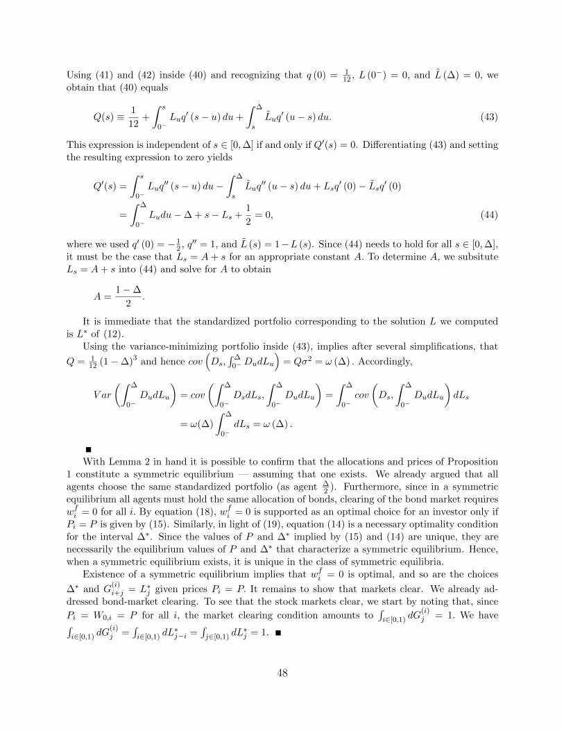
Using (41) and (42) inside (40) and recognizing that q (0) = 112 , L (0−) = 0, and L (∆) = 0, we

obtain that (40) equals

Q(s) ≡ 1

12+

∫ s

0−Luq

′ (s− u) du+

∫ ∆

sLuq

′ (u− s) du. (43)

This expression is independent of s ∈ [0,∆] if and only if Q′(s) = 0. Differentiating (43) and settingthe resulting expression to zero yields

Q′(s) =

∫ s

0−Luq

′′ (s− u) du−∫ ∆

sLuq

′′ (u− s) du+ Lsq′ (0)− Lsq′ (0)

=

∫ ∆

0−Ludu−∆ + s− Ls +

1

2= 0, (44)

where we used q′ (0) = −12 , q′′ = 1, and L (s) = 1−L (s). Since (44) needs to hold for all s ∈ [0,∆],

it must be the case that Ls = A+ s for an appropriate constant A. To determine A, we subsituteLs = A+ s into (44) and solve for A to obtain

A =1−∆

2.

It is immediate that the standardized portfolio corresponding to the solution L we computedis L∗ of (12).

Using the variance-minimizing portfolio inside (43), implies after several simplifications, that

Q = 112 (1−∆)3 and hence cov

(Ds,

∫ ∆0− DudLu

)= Qσ2 = ω (∆) . Accordingly,

V ar

(∫ ∆

0−DudLu

)= cov

(∫ ∆

0−DsdLs,

∫ ∆

0−DudLu

)=

∫ ∆

0−cov

(Ds,

∫ ∆

0−DudLu

)dLs

= ω(∆)

∫ ∆

0−dLs = ω (∆) .

With Lemma 2 in hand it is possible to confirm that the allocations and prices of Proposition1 constitute a symmetric equilibrium — assuming that one exists. We already argued that allagents choose the same standardized portfolio (as agent ∆

2 ). Furthermore, since in a symmetricequilibrium all agents must hold the same allocation of bonds, clearing of the bond market requireswfi = 0 for all i. By equation (18), wfi = 0 is supported as an optimal choice for an investor only ifPi = P is given by (15). Similarly, in light of (19), equation (14) is a necessary optimality conditionfor the interval ∆∗. Since the values of P and ∆∗ implied by (15) and (14) are unique, they arenecessarily the equilibrium values of P and ∆∗ that characterize a symmetric equilibrium. Hence,when a symmetric equilibrium exists, it is unique in the class of symmetric equilibria.

Existence of a symmetric equilibrium implies that wfi = 0 is optimal, and so are the choices

∆∗ and G(i)i+j = L∗j given prices Pi = P. It remains to show that markets clear. We already ad-

dressed bond-market clearing. To see that the stock markets clear, we start by noting that, since

Pi = W0,i = P for all i, the market clearing condition amounts to∫i∈[0,1) dG

(i)j = 1. We have∫

i∈[0,1) dG(i)j =

∫i∈[0,1) dL

∗j−i =

∫j∈[0,1) dL

∗j = 1.

48

Proof of Proposition 2. Let w∗ (P ) denote the set of optimal wfi solving the maximizationproblem (17) when the price in all markets is P. We first note that the assumption that no symmetricequilibrium exists implies that there exists no P such that 0 ∈ w∗(P ). (If such a P existed, thenwe could simply repeat the arguments of Proposition 1 to establish the existence of a symmetricequilibrium with price Pi = P, and interval choice ∆i = ∆∗(P )).

We next show that since there exists no P such that 0 ∈ w∗(P ), it follows that w∗(P ) cannotbe single-valued for all P. We argue by contradiction. Suppose to the contrary that w∗(P ) issingle-valued. Since the theorem of the maximum implies that w∗(P ) is a upper-hemicontinuouscorrespondence, it follows that w∗(P ) is actually a continuous function. Inspection of (17) showsthat w∗(1) = 1. Moreover, as P → −∞, the optimal solution to (17) becomes negative: w∗ (−∞) <0. Then an application of the intermediate value theorem gives the existence of P such thatw∗ (P ) = 0, a contradiction.

Combining the facts that a) there exists no P such that 0 ∈ w∗(P ), b) w∗(P ) is multi-valued forat least one value of P , and c) w∗(P ) is upper-hemicontinuous, implies that there exists at least oneP such that {w1, w2} ∈ w∗(P ) with w1 > 0 and w2 < 0. An implication of the necessary first-ordercondition for the optimality of the interval choice ∆∗ (P ) is that ∆∗ (P ) is also multi-valued with∆1 < ∆2. Furthermore, since prices in all locations are equal, the (standardized) optimal portfolioof an agent choosing ∆k is the variance-minimizing portfolio of Proposition 1, denoted L∗,k.

From this point onwards, an equilibrium can be constructed as follows. By definition, thetuples

{∆1, w1, dL

∗,1} and{

∆2, w2, dL∗,2} are optimal. Hence it only remains to confirm that asset

markets clear. Define π ≡ − w2w1−w2

∈ (0, 1). By construction, πw1 + (1− π)w2 = 0 and, therefore,

if in every location π agents choose{

∆1, w1, dL∗,1} and the remaining fraction (1− π) choose{

∆2, w2, dL∗,2} , then the bond market clears by construction. To see that the stock markets clear,

we start by noting that, since Pi = W0,i = P , the market clearing condition for stock i amounts to

π

∫[0,1]

dL∗,1j−i + (1− π)

∫[0,1]

dL∗,2j−i = 1,

which holds because L∗,kj for k ∈ {1, 2} is a measure on the circle.We prove next that symmetric and asymmetric equilibria (with different prices) cannot co-exist.

Inspection of (17) shows that the optimal wfi is increasing in P in the sense that if P1 < P2 thenw1 < w2 for any w1 ∈ w∗(P1) and w2 ∈ w∗(P2).31 Accordingly, if a symmetric equilibrium exists,i.e., if there is a P such that 0 ∈ w∗(P ) then there cannot exist P 6= P with the property that{w1, w2} ∈ w(P ) and yet w1 > 0 and w2 < 0, which is a requirement for the existence of anasymmetric equilibrium. Hence symmetric and asymmetric equilibria cannot co-exist. The factthat w∗(P ) is an increasing correspondence also implies that asymmetric equilibria are essentiallyunique, in the sense that asymmetric equilibria associated with different equilibrium prices cannotco-exist.

Remark 1 The existence proof of an asymmetric equilibrium (when a symmetric equilibrium failsto exist) obtains also in the presence of the leverage constraint (23) that we introduce in Section 5.

Proof of Proposition 3. Conjecture first that in equilibrium Pj = P for all j and letπ ∈ [0, 1] denote the fraction of funds invested in the local market. Assuming that a given investor

31To see that this statement is correct, consider the maximum V (P,wfi ) of the maximand in (17) over ∆

and note that it cross-partial derivative with respect to P and wfi is positive: ∂P∂wfiV (P,wfi ) > 0.

49

chooses N = 2 (that is, chooses to invest in her own location and another location at distance d),equation (4) allows the computation of the minimal portfolio variance:

ω (d) = σ2 minπ

{(π2 + (1− π)2

) 1

12+ 2π (1− π)

(1

12− d (1− d)

2

)}(45)

= σ2

(1

12− 1

4d (1− d)

).

The optimal distance d for an investor choosing N = 2 satisfies a first-order condition similarto equation (19), namely

−γ2

(1− wf

)2 ω′ (d)

ω2 (d)= κf ′ (d) . (46)

Since ω′ (d) = 0 when and only when d = 12 , and f ′ (d) = 0, it follows that d = 1

2 is optimal foran investor choosing N = 2. Hence the minimal portfolio variance of an investor choosing N = 1is equal to ω (0) = σ2

12 , while the minimal portfolio variance for an investor choosing N = 2 is

ω(

12

)= σ2

48 . Assuming that the equilibrium is of the asymmetric, location-invariant type, we canuse equation (17) to express the indifference between the choices N = 1, respectively N = 2 andd = 1

2 , as

Pwf1 +(

1− wf1)− γ

2

(1− wf1

)2ω (0) = Pwf2 +

(1− wf2

)− γ

2

(1− wf2

)2ω

(1

2

)− κf0. (47)

Using the first-order conditions for leverage

1− P = γ(

1− wf2)ω

(1

2

)= γ

(1− wf1

)ω (0) (48)

inside (47) yields — after some simplifications — the equilibrium price (24).To verify that the postulated equilibrium is indeed an equilibrium, we proceed as in the proof

of Proposition 2. For P (κ) to be an equilibrium price in all locations, it must also be case that

1 − wf1 ≤ 1 ≤ 1 − wf2 , so that setting π =wf2

wf2−wf1

> 0 ensures market clearing (of bond markets

and all risky asset markets). In light of (48), the requirement 1−wf1 ≤ 1 ≤ 1−wf2 is equivalent toP ∈

[1− γω (0) , 1− γω

(12

)]. This requirement is satisfied as long as κ ∈ (κ1, κ2).

Lemma 3 Consider an investor located at i /∈[−k

2 ; k2], and therefore investing in markets [i −

∆2 , i + ∆

2 ]. Suppose that P (x) is continuously differentiable everywhere on [i − ∆2 , i + ∆

2 ]. With

dX(i)l the number of shares purchased on the account of an investor at i in market l and j ≡ i− ∆

2 ,

X(i)

j+∆=

1

γω(∆) [1− 1− ∆

2

(Pj + Pj+∆

)−∫ j+∆

jPu du

]. (49)

Furthermore, the function X is given by

X(i)j+l =

P ′j+lγσ2

+X(i)

j+∆

1−∆ + 2l

2+

1

1− ∆

Pj+∆ − Pjγσ2

. (50)

50

If an investor is located at i ∈ [−k2 ,

k2 ] and only invests in market i then the respective demand for

risky asset i is given by

X(i)i =

1

γω (0)(1− Pi) . (51)

Proof of Lemma 3. Notice that optimization problem of agent i is equivalent to

maxX

Pi +

∫ j+∆

j−(1− Pu) dXu −

γ

2V ar

(∫ j+∆

j−DudXu

)(52)

Thus, the first-order condition requires that

γ cov

(Ds,

∫ j+∆

j−DudXu

)= 1− Ps (53)

for all s ∈[j, j + ∆

]. Letting q (d) be defined as in Lemma 2 we can rewrite (53) as∫ s

j−q (s− u) dXu +

∫ j+∆

sq (u− s) dXu =

1− Psγσ2

. (54)

Let X (s) = X(j + ∆

)−X (s) and integrating by parts we obtain∫ s

j−q (s− u) dXu = X (s) q (0)−X

(j−)q (s) +

∫ s

jXuq

′ (s− u) du (55)∫ j+∆

sq (u− s) dXu = X (s) q (0)− X

(∆)q (∆− s) +

∫ j+∆

sXuq

′ (u− s) du (56)

Substituting (55) and (56) into (54), recognizing that q (0) = 112 , X (j−) = 0, and X

(j + ∆

)= 0,

we obtain

1

12X(j + ∆

)+

∫ s

jXuq

′ (s− u) du+

∫ j+∆

sXuq

′ (u− s) du =1− Psγσ2

. (57)

Since this relation must hold for all s, we may differentiate both sides of (57) to obtain∫ s

jXuq

′′ (s− u) du−∫ j+∆

sXuq

′′ (u− s) du+Xsq′ (0)− Xsq

′ (0) = − P′s

γσ2. (58)

This equation holds for all s ∈ (j, j + ∆). Noting that q′′ = 1, q′ (0) = −12 , X (s) = X

(j + ∆

)−

X (s), and using (58) to solve for Xs yields

Xs =

∫ j+∆

jXudu+

(s− j +

1

2− ∆

)X(j + ∆

)+P ′sγσ2

. (59)

51

Integrating (59) from j to j + ∆ and solving for∫ j+∆j Xudu leads to

∫ j+∆

jXudu =

1

1− ∆

[X(j + ∆

)∆

(1− ∆

2

)+P(j + ∆

)− P (j)

γσ2

], (60)

so that

Xs =1

1− ∆

[X(j + ∆

)∆

(1− ∆

2

)+P(j + ∆

)− P (j)

γσ2

]+(

s− j +1

2− ∆

)X(j + ∆

)+P ′sγσ2

. (61)

Evaluating (57) at s = j + ∆, and noting that q′ (s) = −12 + s leads to

1

12X(j + ∆

)+

∫ j+∆

jXu

[−1

2+(∆− u

)]du =

1− Pj+∆

γσ2. (62)

An implication of (59) is that Xu = Xj +P ′u−P ′jγσ2 + X

(j + ∆

)u. Using this expression for

Xu inside (62), carrying out the requisite integrations and using integration by parts to express∫ j+∆j

(P ′uγσ2

)u du =

Pj+∆

γσ2 (j + ∆)− Pjγσ2 j −

∫ j+∆j

Puγσ2du, leads (after some simplifications) to

X(j + ∆

)( 1

12+

∆3

6− ∆2

4

)−

∆(1− ∆

)2

(Xj −

P ′jγσ2

)−Pj+∆ − Pj

2γσ2+

∫ j+∆

j−

Pu − Pjγσ2

du

=1− P∆

γσ2. (63)

Finally, evaluating (59) at j gives(Xj −

P ′jγσ2

)=

∫ j+∆

jXudu+

(1

2− ∆

)X(j + ∆

). (64)

Equations (60), (63), and (64) are three linear equations in three unknowns. Solving forX(j+∆)and using the definition of ω

(∆)

leads to (49). Equation (61) simplifies to (50). Finally, (51) is adirect consequence of (53) when ∆ = 0.

Proof of Proposition 4. For any j ∈(k2 ,

12

]and l ∈

(− ∆

2 ,∆2

), we have from Lemma 3:

X(j)

j− ∆2

=P ′j− ∆

2

γσ2+Pj− ∆

2

− Pj+ ∆

2

γσ2(1−∆)+

1−∆

2X

(j)

j+ ∆2

dX(j)j+l =

(P ′′j+lγσ2

+X(j)

j+ ∆2

)dl

X(j)

j+ ∆2

−X(j)(j+ ∆

2

)− = −P ′j+ ∆

2

γσ2−Pj− ∆

2

− Pj+ ∆

2

γσ2(1−∆)+

1−∆

2X

(j)

j+ ∆2

.

52

Specialize the first equation to j = 12 + ∆

2 , the second to j = 12 − l for all l ∈

(− ∆

2 ,∆2

), and the

third to j = 12 −

∆2 and aggregate to obtain the total demand for asset 1

2 :

1 =1−∆

2X

( 12

+ ∆2

)12

+∆+

1−∆

2X

( 12− ∆

2)

12

+

∫ ∆2

− ∆2

X( 1

2−l)

12−l+ ∆

2

dl +P ′′1

2

γσ2∆ +

P 12−∆ + P 1

2+∆ − 2P 1

2

2γσ2(1−∆).

Suppose now that Pj ≥ 1 − γω(∆) on[

12 −∆, 1

2 + ∆], with strict inequality on a positive

measure set. It then follows from equation (49) that X(j)

j+ ∆2

≤ 1, so that

0 <P ′′1

2

γσ2∆ +

P 12−∆ + P 1

2+∆ − 2P 1

2

2γσ2(1−∆).

This inequality contradicts the assumption that P is maximized at 12 .

Proof of Proposition 5. We adopt a guess-and-verify approach. We start by noting that the

beginning-of-period wealth of investor i at time t+ 1 is Wt+1,i ≡∫ 1

0 (Pt+1,j +Dt+1,j) dX(i)t,j +X

(i)B,t.

We then conjecture that, as long as

F (∆) =M

γ+γ

2

(r

1 + r − ρ

)2

(1− ρ)2 ω (∆t) (65)

for some M > −γ2

2

(r

1+r−ρ

)2(1− ρ)2 ω (∆u), (ii) and (iii) obtain. We show at the end that the

function F can be chosen to ensure (i).

We also conjecture and verify that investors’ holdings of risky assets X(i)t,j coincide with G

(i)t,j of

Proposition 1, and that their bond holdings equal

X(i)B,t = Wt,i − (1 + r)P t,i − rΦt, (66)

where P t,i ≡∫ 1

0 Pt,jdX(i)t,j is the average price that investor i pays for her portfolio. Here, to simplify

notation, we defined Φt ≡ Φ1ω(∆t) + Φ0.We first ensure that with these postulates markets clear. Clearly, all risky markets clear,

since the holdings of risky assets are the same as in Proposition 1. To show that bond marketsclear, we proceed inductively. First we note that investors are endowed with no bonds at time

zero. Hence∫ 1

0 X(i)B,−1di = 0 and therefore

∫ 10 W0,idi =

∫ 10 (P0,i +D0,i) di. Next we postulate that∫ 1

0 X(i)B,t−1di = 0, so that

∫ 10 Wt,idi =

∫ 10 Pt,idi +

∫ 10 Dt,jdj. Integrating our postulate (66) for X

(i)B,t

across all investors, we obtain∫ 1

0X

(i)B,tdi =

∫ 1

0Wt,idi− (1 + r)

∫ 1

0P t,idi− rΦt. (67)

We next note that that (a)∫ 1

0 Dt,jdj = 1, by construction of the dividend process; (b)∫ 1

0 Wt,idi =∫ 10 Pt,idi+

∫ 10 Dt,jdj = r−1−Φt+1, using the induction hypothesis, (31), and (a); and (c)

∫ 10 P t,idi =∫ 1

0 Pt,idi = r−1 − Φt. Using these three facts, it follows immediately that the right-hand side of(67) is zero, so that the bond market clears.

53

If investors set their bond holdings according to (66), then their budget constraint implies aconsumption of

ct,i = Wt,i −1

1 + rX

(i)B,t − P t,i − Ft. (68)

Using the definition of Wt,i and market clearing condition for bond holdings inside (68), and inte-

grating across i implies that the market for consumption goods clears:∫ 1

0 ct,idi = 1− Ft.Having established market clearing given the postulated policies and prices, we next turn to

optimality. Equation (68) implies

ct+1,i − ct,i = Wt+1,i −Wt,i −1

1 + r

(X

(i)B,t+1 −X

(i)B,t

)−(P t+1,i − P t,i

)− (Ft+1 − Ft)

=

(r

1 + r

)(Wt+1,i −Wt,i) +

r

1 + r(Φt+1 − Φt)− (Ft+1 − Ft) , (69)

where the second line follows from (66). We next use the definition of Wt,i and (66) to obtain

Wt+1,i −Wt,i =

∫ 1

0(Pt+1,j +Dt+1,j) dX

(i)t,j +X

(i)B,t −Wt,i

=

∫ 1

0(Pt+1,j +Dt+1,j) dX

(i)t,j − (1 + r)P t,i − rΦt. (70)

Substituting (70) into (69) and using (31) and (66) leads to

ct+1,i − ct,i =

(r

1 + r

)[(1 + φ)

∫ 1

0Dt+1,jdX

(i)t,j − (1 + r)φ

∫ 1

0Dt,jdX

(i)t,j − (1− rφ)

∫ 1

0dX

(i)t,j

]− (Ft+1 − Ft) . (71)

Next use the fact Dt+1,j = ρDt,j + (1− ρ) εt+1,j along with φ = ρ1+r−ρ , (1 + φ) ρ = (1 + r)φ, and

(1 + φ) (1− ρ) = (1− rφ) inside (71) to arrive at

ct+1,i − ct,i =

(r

1 + r − ρ

)(1− ρ)

∫ 1

0(εt+1,j − 1) dX

(i)t,j − (Ft+1 − Ft) . (72)

Having established (72), the dynamics of agent i’s consumption under our postulate, we nextturn attention to the Euler equations, starting with the bond Euler equation

1 = β (1 + r)Ete−γ(ct+1,i−ct,i). (73)

Substituting (72) into (73) and noting that∫ 1

0 (εt+1,j − 1) dX(i)t,j is normally distributed with mean

zero and variance ω (∆t) gives

1 = β (1 + r) eγ2

2

(r

1+r−ρ

)2(1−ρ)2ω(∆t)−γFtEt

(eγFt+1

). (74)

54

Now suppose that for any r and a given desired distribution Ψ (∆) we set

Ft (∆t; r) =M

γ+γ

2

(r

1 + r − ρ

)2

(1− ρ)2 ω (∆t) . (75)

Then equation (74) can be written as (30). Since (1 + r)Eeγ2

2

(r

1+r−ρ

)2(1−ρ)2ω(∆)

is equal to 1 whenr = 0 and increases monotonically to infinity as r increases, it follows that there exists a uniquepositive r such that equation (30) holds. For that value of r, all investors’ bond Euler equationsare satisfied.

Finally, we need to determine Φt so as to ensure that the Euler equations for risky assets hold,i.e., that

Pt,j = βEt

[e−γ(ct+1,i−ct,i) (Pt+1,j +Dt+1,j)

]. (76)

To that end, we use (31) and (28) to express (76) as

1

r−Φt+φ(Dt,j−1) = βEt

[e−γ(ct+1,i−ct,i)

(1

r− Φt+1 + (1 + φ) (ρDt,j + (1− ρ) εt+1,j)− φ

)]. (77)

We next note that

βEt

[e−γ(ct+1,i−ct,i)

](1 + φ) ρDt,j =

(1 + φ) ρ

1 + rDt,j = φDt,j (78)

using (73). Equation (78) simplifies (77) to

1

r− Φt − φ = βEt

[e−γ(ct+1,i−ct,i)

(1

r− Φt+1 + (1 + φ) (1− ρ) εt+1,j − φ

)]=

1

r(1 + r)− βEt

[e−γ(ct+1,i−ct,i)Φt+1

]+

1

1 + r(−φ+ (1 + φ) (1− ρ)) (79)

+ (1 + φ) (1− ρ)βEt

[e−γ(ct+1,i−ct,i)(εt+1,j − 1)

].

Using (72), Stein’s Lemma, the fact that cov(∫ 1

0 (εt+1,j − 1) dX(i)t,j , εt+1,j

)= ω (∆) (see Proposition

1), and (73) implies

βEt

[e−γ(ct+1,i−ct,i)εt+1,j

]=

1− γ r1+r−ρ (1− ρ)ω (∆t)

1 + r. (80)

Substituting (80) into (79) gives linear equations in Φ0 and Φ1, solved by (32), respectively (33).To complete the proof of the claim that ∆t is chosen optimally, we provide an explicit example

of a family of functions for Ft (∆) that has the desired properties. To start, we compute the valuefunction of an investor adopting the policies of Proposition 5. Equation (73) along with (72) imply

55

that

V (Wt,i,∆t) = −1

γ

∑t≥0

βtEt[e−γct,i

]= −1

γe−γc0,i

1 +∑t≥1

βtEt

[e−γ

∑t−1m=0(cm+1,i−cm,i)

]= −1

γe−γc0,i

∑t≥0

(1 + r)−t = −1 + r

γre−γc0,i .

In turn, equations (66), (68), and (75) imply

V (Wt,i,∆t) = −1 + r

γre−

γr1+r

Wt,i+z(∆t), (81)

where zt (∆t) ≡ − r1+rγΦt +M + γ2

2

(r

1+r−ρ

)2(1− ρ)2 ω (∆t) .

Next we suppose that we no longer impose that the investor choose ∆ = ∆t, (where ∆t isthe time-t random draw of ∆ that we imposed in Proposition 5). Instead ∆ is chosen optimally.However, prices are still given by Pt,j (∆t, Dt,j) from equation (31). We will construct a functionκtgt (∆) that renders the choice ∆ = ∆t optimal at the total cost specified in (75).

Throughout we let X(i)t (∆; ∆t) denote the optimal number of total risky assets chosen by

investor i, and assuming that that investor chooses ∆ and prices are given by Pt,j (∆t, Dt,j) . Forfuture reference, we note that by construction of the price function Pt,j (∆t, Dt,j) it follows that

X(i)t (∆t; ∆t) = 1. Using (81) the first order condition characterizing an optimal ∆ is

F ′t (∆) = h (∆; ∆t) ,

where

h (∆; ∆t) = − 1

1 + r

γ

2

(r

1 + r − ρ

)2

(1− ρ)2(X

(i)t (∆; ∆t)

)2ω′ (∆) . (82)

Next we fix a value of ∆t and we simplify notation by writing h (∆) rather than h (∆; ∆t) . Wealso let q (x) denote some continuous function with q (0) = 1 and q (x) > 1 for x > 0. Let η ∈ [0, 1],take some positive (small) ε < ∆t

2 , and consider the function

F ′t (∆) =

∆ε ηh (ε) for ∆ ≤ εηh (∆) for ∆ ∈ (ε,∆t − ε]ηh (∆t − ε) ∆t−∆

ε + h (∆t)∆−∆t+ε

ε for ∆ ∈ (∆t − ε,∆t]h (∆) q(∆) for ∆ > ∆t + ε.

. (83)

By construction, F ′t (0) = 0 and F ′t (∆) is continuous and increasing in ∆. More importantly,F ′t (∆t) = h (∆t) , and hence ∆ = ∆t satisfies the necessary first order condition (82). Moreover,since F ′t (∆) < (>)h (∆) for ∆ < (>)∆t, it follows that ∆ = ∆t is optimal for any ε > 0 andη ∈ [0, 1]. Finally,

limε→0

∫ ∆t

0F ′t (∆) = η

∫ ∆t

0h (x) dx > 0. (84)

Now suppose that nature draws ∆t = ∆u > 0. By choosing M that is sufficiently close to

56

−γ2

(r

1+r−ρ

)2(1− ρ)2 ω

(∆)

it follows that

0 <M

γ+γ

2

(r

1 + r − ρ

)2

(1− ρ)2 ω (∆u) <

∫ ∆u

0h (x) dx. (85)

Combining equations (84) and (85) it follows that for sufficiently small ε > 0 there exists someη ∈ [0, 1] so that∫ ∆u

0F ′t (x) dx =

M

γ+γ

2

(r

1 + r − ρ

)2

(1− ρ)2 ω (∆u) > 0. (86)

Hence, when ∆t = ∆u the cost function κtgt (∆) renders ∆ = ∆u, while also satisfying (75).The same argument implies that for any value of ∆t that satisfies

0 <M

γ+γ

2

(r

1 + r − ρ

)2

(1− ρ)2 ω (∆t) <

∫ ∆t

0h (x) dx, (87)

there exists η ∈ [0, 1] and sufficiently small ε > 0 such that the optimal ∆ coincides with ∆t, and

(75) holds. Continuity of ω (∆t) and of∫ ∆t

0 h (x) dx in ∆t implies that as long as ∆ is sufficientlyclose to ∆u, there always exists η ∈ [0, 1] and ε > 0 (both depending on the random draw ∆t) suchthat ∆ = ∆t is optimal and (75) holds.

Proof of Proposition 6. Parts (i)–(iii) are proved in the main body of the text. Part (iv)comes down to noticing that

cov (ez, z) > 0 (88)

for any random variable z — in particular, for z = ω(∆). The second statement of (iv) followsfrom the first and Jensen’s inequality applied to the convex function ω.

C An interpretation of participation costs

Throughout the paper we maintain the assumption that participation in “distant” markets incursparticipation costs. In this appendix32 we discuss how these costs could arise as information-acquisition costs that permit an investor to avoid the lower net returns earned by an investorunfamiliar with the asset class. Indeed, we wish to re-emphasize that we construe the notion ofdistance broadly, as a stand-in for the level of familiarity of investors in one location with all aspectsof the financial environment in another. We also wish to emphasize that our notion of locations ismeant to be very broad, in particular encompassing asset classes that may be especially opaque touninformed investors (e.g., mortgage pools and small stocks in distant countries).

32This appendix borrows from Garleanu et al. (2013). We present a self-contained version of the model tokeep the effort required of the interested reader to a minimum. Another related paper that derives portfolioconcentration as a result of endogenous information acquisition is Van Nieuwerburgh and Veldkamp (2010).

57

C.1 Regular firms and common investors

Timing and the set of locations are the same as in Section 3. In each location there are measure-onecontinua of investors and firms, but both are of two types: Investors are either “common investors”or “swindlers”, while firms are either “regular” or “fraudulent”.

Common investors in each location constitute a fraction ν ∈ (0, 1) of the population in thatlocation. They are identically endowed with an equal-weighted portfolio of all regular firms in thatlocation i. The total measure of regular firms in each location is also ν. All regular firms in locationi produce the same random output: Dik = Di, where k identifies the firm. The dividend is givenby equation (3), as in the paper:

Di ≡ 1 +

(Bi −

∫ 1

0Bjdj

). (89)

Swindlers are a fraction 1 − ν of the population in each location. Each swindler is endowedwith the entirety of shares (normalized to one) of one fraudulent firm. Fraudulent firms producezero output (Dik = 0).

For every firm in every location, there is a market for shares where any investor can submit ademand. As before, there exists a market for the riskless bond, available in zero net supply. Sinceinvestors don’t consume at time zero, we use the bond as the numeraire, and normalize its price toone (r = 0).

C.2 Budget constraints

Letting Bci denote the amount that a common investor in location i invests in riskless bonds, andXcijk denote a bivariate signed measure giving the number shares of firm k in location j she invests

in, the time-one wealth of a common investor located in i is given by

W ci1 ≡ Bci +

∫j∈L

∫k∈[0,1]

Djk dXcijk. (90)

The first term on the right hand side of (90) is the amount that the investor receives from her bondposition in period 1, while the second term captures the portfolio-weighted dividends of all thefirms that the investor holds. The time-zero budget constraint of a common investor in location iis given by

Bci +

∫j∈L

∫k∈[0,1]

Pjk dXcijk =

1

ν

∫k∈[0,1]

Pikρikdk, (91)

where ρik is an indicator function taking the value one if the firm k in location i is a regular firmand zero otherwise, and Pjk refers to the price of security k in location j. The left-hand side of (91)corresponds to the sum of the investor’s bond and risky-security spending, while the right-hand sidereflects the value of the (equal-weighted) portfolio of regular firms the investor is endowed with.

C.3 Signals

Each investor may obtain a signal of the type — regular or fraudulent — of every firm in everylocation. The precision of these signals depends on the locations of the investor and the firm.

58

Specifically, we assume that each fraudulent firm in every location is assigned in an i.i.d. fashiona uniformly distributed index u ∈ [0, 1 − ν], which reflects the difficulty with which it can beidentified as fraudulent. This index is not observed by anyone.

After the index is drawn, investors in every location i may obtain a signal about each firm inlocation j. (All investors in i who choose to become informed obtain the same signal about any givenfirm.) This signal characterizes the firm as either regular or fraudulent. The signal is imperfect. Itcorrectly identifies every regular firm as such. However, it fails to identify all fraudulent firms: itcorrectly identifies a fraudulent firm that has drawn an index u with probability πu and misclassifiesit as regular with probability 1− πu. Note that we take πu independent of i and j.

We introduce the index u to obtain a heterogeneous distribution of the demand for the sharesof fraudulent firms in the same location by investors in other locations. We assume that for some(positive-measure) set of values u πu = 1, i.e., there exist in every location a positive measure offraudulent firms that are correctly classified as fraudulent by all informed agents. No one knows,however, the identity of these firms before trading takes place. (Even conditional on prices andeach agent’s own trades, only the swindler can infer the u of her own firm in equilibrium).

Given this setup, Bayes’ rule implies that the probability that a firm in location j is regulargiven that investor i’s signal identifies it as regular is given by

p ≡ ν

ν +∫ 1−ν

0 (1− πu) du. (92)

The law of large numbers implies then that p can also be interpreted as the fraction of firms ina given location j that are regular, given that the signal of investor i has identified them as regular.

The signals are costly. Specifically, the investor in location i can acquire signals about all thefirms in a given location j, by paying exactly the same “participation costs” that we assume inSection 3.2. We denote the cost function by F .

C.4 Earnings manipulation and swindler’s problem

We next introduce an assumption whose sole purpose is to ensure endogenously that agents do notshort fraudulent shares. Before proceeding, we note that one can dispense with all the assumptionsof this section, by simply imposing a no-shorting constraint.

Specifically, we assume that swindlers have the ability to manipulate the earnings of fraudulentfirms. A swindler l in location i has the ability to borrow any amount Lil ≥ 0 of her choosing at time0, divert these funds into the firm, and report earnings equal to Lil in period 1. (Equivalently, wecould assume that the swindler can take an action to produce earnings Lil by incurring a personalnon-pecuniary cost of effort, which would have a value Lil in monetary terms.)

The budget constraint of a swindler is similar to (91) except that ν−1∫k∈[0,1] Pikρ(i,k)dk is

replaced by Pil:

Bsil +

∫j∈L

∫k∈[0,1]

PjkdXsiljk = Pil. (93)

Note that, as before, the notation allows investors’ portfolios to have atoms, which is furtheruseful here because, in equilibrium, swindlers optimally hold a non-infinitesimal quantity of sharesof their own firms. We denote the post-trade number of shares held by the swindler who owns firml in location i by Sil = dXsil

il .

59

The time-1 wealth of a swindler is

W sil1 ≡ Bsil +

∫j∈L

∫k∈[0,1]

DjkdXsiljk + Lil

(Sil − 1

). (94)

The difference with (90) is the term Lil(Sil − 1

), which represents the swindler’s consumption

gains when performing a diversion Lil, while owning a post-trade number of shares in her companyequal to Sil. This increase is intuitive. If Sil − 1 < 0, i.e., if the swindler reduces her ownershipof shares by being a net seller, then she has no incentive to perform earnings diversion sinceshe will recover only a fraction of her personal funds that she diverts into the company; thus

Lil = 0. If, however, the swindler is a net buyer of her own security(Sil − 1 > 0

), then the

ability to manipulate earnings becomes infinitely valuable, since Lil can be chosen arbitrarily large.Intuitively, the swindler can report arbitrarily large profits at the expense of outside investors whohold negative positions (short sellers) in the fraudulent firm. As a consequence, in equilibriumall other investors optimally refrain from shorting, even when they know for sure that the firm isfraudulent. The reasoning is as follows: With positive probability πu = 1; accordingly all investors’signals identify the fraudulent firm as such, and investors do not find it optimal to submit a positivedemand for that firm in equilibrium. Therefore, any prospective shorter understands that any shortposition that she establishes implies Sil > 1, and is (unboundedly) loss-making. Since the qualityof the signal (u) is not observed by anyone33, a prospective shorter must assign positive probabilityto such an occurrence, and hence avoids short-selling.

Before proceeding, we reiterate that our earnings-manipulation assumption serves only as adeterrent to shorting, and is intentionally stylized so as to expedite the presentation of the resultsthat follow. In reality there are many other reasons why investors are deterred from short sellingfirms with tightly controlled float, such as “short squeezes”, which we do not model here.34 Theexact nature of the shorting deterrent is inconsequential for our results. (See, e.g., Lamont (2012)for an empirical study documenting various short-selling deterrence mechanisms employed by firms.)

C.5 Optimization problem

All investor are maximizing a CARA utility with parameter γ over time-1 wealth.Common investors are price takers. Taking the interest rate, the prices for risky assets, and

the actions of the swindlers as given for all firms in all locations, a common investor maximizes herexpected utility subject to (91). The investor conditions on her own information set Fi (i.e., onher signals about every security), as well as on the prices of all securities in all markets.

The problem of the swindler is similar to the one of the common investor with two exceptions:a) she takes into account the impact of her trading on the price of her stock, and b) she needs todecide whether to manipulate the earnings of her company. Similarly to a common investor, theswindler who owns firm l in location i maximizes her utility over Bsil and dXsil

jk subject to thebudget constraint (93).

33In equilibrium only the swindler can infer the u of her own firm.34A short squeeze refers to the possibility of cornering the shorting market by restricting the amount of

securities that are available for lending and forcing short sellers to close out their positions. Short squeezescan be detrimental to short sellers. We do not model these deterrence mechanisms here since they wouldrequire the introduction of more trading periods in the model.

60

C.6 Equilibrium

An equilibrium is a collection of prices Pi for all risky assets, asset demands, and bond holdingsexpressed by all investors in all locations, such that: 1) Markets for all securities clear: ν

∫i∈L dX

cijk+∫

i∈L∫ 1l=ν dX

siljk = 1 for all j, k; 2) Risky-asset and bond holdings,

{Xcijk, B

ci}

, are optimal for regular

investors in all locations given prices and the investors’ expectations; 3) Optimal bond holdingsBsil, diversion amounts Lsil, and asset holdings for all securities Xsil

jk (including a swindler’s own

holdings of her own firm Sil) are optimal for swindlers given their expectations; 4) All investorsupdate their beliefs about the type of stock k in location j by using all available information tothem — prices, interest rate, and private signals — and Bayes’ rule, whenever possible.

Our equilibrium concept contains elements of both a rational expectations equilibrium and aBayes-Nash equilibrium. All investors make rational inferences about the type of each securitybased on their signals, the equilibrium prices, and the interest rate, by using Bayes’ rule and takingthe optimal actions of all other investors (regular and swindlers) in all locations as given. Theassumption of a continuum of regular investors implies that they are price takers in all markets. Informing dividend anticipations about a given security, they take prices and the optimal diversionstrategies of swindlers as given.

Swindlers, on the other hand, are endowed with the shares of a fraudulent company and canmanipulate its earnings. Thus they take into account the impact of their trades on the securitythey are trading. In formulating a demand for their security, swindlers have to consider howdifferent prices might affect the perceptions of other investors about the type of their security. Asis standard, Bayes’ rule disciplines investors’ beliefs only for demand realizations that are observedin equilibrium. As is usual in a Bayes-Nash equilibrium, there is freedom in specifying how out-of-equilibrium prices affect investor posterior distributions of security types.

We note that the distinction between regular investors, who are rational price-takers andswindlers who are strategic about the impact of their actions on the price of their firm is help-ful for expediting the presentation of results, but not crucial. We can show35 that our equilibriumconcept is the limit (as the number of traders approaches infinity) of a sequence of economies withfinite numbers of traders — both regular and swindlers — who are all strategic about their priceimpact and rational about their inferences, as in Kyle (1989).

C.7 Non-participation

We are finally ready to state the result of this appendix, which states that non-participation canarise as the result of a choice not to obtain signals about given markets. As in Section 3, we focusfor simplicity on location invariance.

Proposition 7 Consider an equilibrium to the economy in Section 3, defined by the price P and

the share holdings X(i)j . Consider also the class of asymmetric-information economies, defined in

this appendix, that are indexed by ν and obey the restrictions γ(ν) = γ/ν, F = νF , and p(ν)/νdecreases in ν with limν→0 p(ν)/ν =∞.

Then there exists a value ν > 0 such that, as long as ν ≤ ν, an equilibrium exists in theasymmetric-information economy that exhibits the following properties.

(i) All prices in location i are equal, Pik = Pi = P = pP .

35See Garleanu et al. (2013) for details.

61

(ii) There is neither shorting nor dividend manipulation in equilibrium— in particular, of fraud-ulent firms.

(iii) If an investor i in the participation-cost economy participates in a set Si of locations, thenthe same investor acquires signals for locations Si and no others, and only trades in theselocations; in fact, the share holdings are proportional (excluding swindler’s holdings of ownfirm share):∫

k∈LdXci

jk =

∫k∈L

dXsiljk =

ν

pdX

(i)j . (95)

Proposition 7 provides an information-theoretic interpretation of participation costs. The in-vestors in the main body of the paper can be thought of as acting in an environment in whichthey have the following choice. They can either pay a “participation” cost — exactly the same asspecified in Section 3.2 — to learn informative signals of the types of securities in a given location,or simply limit their investments in that location to uninformed (index) portfolios. According toProposition 7, in case their information advantage in markets where they are informed is sufficientlylarge compared to markets where they are uninformed, then it is optimal to allocate their limitedcapital exclusively in locations where they are not subject to an informational disadvantage, thusforegoing some diversification benefits. Put differently, they only invest in a location when theyhave paid the cost to become informed about it.

C.8 Proof of Proposition 7

Proof. We structure the proof in two steps. We start by assuming that no shorting or divi-dend manipulation is possible, and verify that the prescribed prices and portfolios constitute anequilibrium. We then check that property (ii) obtains as a result of optimal behavior.

Step 1. Suppose first that investors in the asymmetric-information economy (AIE) obtainsignals and invest in the same locations Si that the investors in the base-case, participation-costeconomy (PCE) choose to participate in. We note that a bad signal identifies a firm as fraudulentfor sure, and therefore the investor does not purchase any share in such a firm. Since the signalson any market j contain noise (so that every firm has the same probability of being misclassified),it is optimal to allocate the funds in location j in an equal way across the firms that are identifiedas regular. In particular, letting Ki

j be the set of firms in location j for which agent i’s signal ispositive, the quantity

dZij ≡∫k∈Ki

j

ρjkdXcijk (96)

is deterministic and equal to

dZij = p

∫k∈Ki

j

dXcijk ≡ p dXci

j . (97)

62

Given the prices, all competitive investors maximize

E

[∫j∈Si

∫k∈Ki

j

(Djk − P

)dXci

jk

]− γ

2V ar

(∫j∈Si

∫k∈Ki

j

Djk dXcijk

)(98)

= E

[∫j∈Si

∫k∈Ki

j

(Dj − P

1

p

)ρjk dX

cijk

]− γ

2V ar

(∫j∈Si

∫k∈Ki

j

Djρjk dXcijk

)

=

∫j∈Si

(E[pDj ]− P

)dXci

j −γ

2V ar

(∫j∈Si

pDjdXcij

)=

∫j∈Si

(E[Dj ]− P ) dZij −γ

2νV ar

(∫j∈Si

DjdZij

). (99)

It consequently follows that, if dX(i)j satisfies the first-order conditions of the investor in the

PCE, dZijk = ν dX(i)j satisfies the first-order conditions of a common investor in the AIE. We

therefore conclude that (95) holds on Si.To verify that the markets for all regular firms clear, it suffices to note that common investors in

i purchase dZcij shares of regular firms in location j, thus ν dX(i)j . The swindlers in i solve exactly

the same problem, in addition to that of trading in their own firm. Consequently the total demand

for regular firms in location j is ν∫i dX

(i)j = ν, the same as the supply. We verify later that markets

clear for the fraudulent firms, as well.We next check that for ν sufficiently low no agent wishes to invest outside Si. The agent’s

concave objective implies that, if a better portfolio existed than the one optimal on Si, then tradingtowards that portfolio would be beneficial. Thus, if W ci

1 is the optimal wealth achievable on Si,then, for t ∈ (0, 1),

E[W ci1 ]− γ

2V ar(W ci

1 )

≤ E[W ci

1 + t

∫j,k

(Djk − P

)dXjk

]− γ

2V ar

(W ci

1 + t

∫j,kDjk dXjk

),

which gives, by letting t go to zero,

E

[∫j,k

(Djk − P

)dXjk

]− γ Cov

(W ci

1 ,

∫j,kDjk dXjk

)≥ 0. (100)

Since both sides are linear in dXjk, and the inequality holds with equality for j ∈ Si, it musthold for at least one location j /∈ Si. (Remember that the agent cannot distinguish between firms

63

in location j.) Thus,

0 ≤ E[∫

k

(Djk − P

)dXjk

]− γ Cov

(W ci

1 ,

∫kDjk dXjk

)= (ν − P )

∫kdXjk − γ Cov

(W ci

1 , νDj

)∫kdXjk

=(ν − pP − γ Cov

(W i

1, νDj

)) ∫kdXjk,

= ν(

1− γ Cov(W i

1, Dj

)− p

νP)∫

kdXjk, (101)

where we used the fact that agent i in the AIE takes the same risky positions (when restricted toSi) as agent i in the PCE, multiplied by ν.

Expression (101), however, is clearly negative as long as P > 0 and p/ν large enough. Thisconclusion represents a contradiction, thus implying that the investor cannot achieve a higher utilityby purchasing (a non-zero measure of) shares located outside Si.

We can write down the investor’s certainty-equivalent as a function of the choice Si by combining(99) with (95) and adding the information costs:

ν

(∫j∈Si

(E[Dj ]− P ) dX(i)j −

γ

2V ar

(∫j∈Si

DjdX(i)j

))− F

= ν

(∫j∈Si

(E[Dj ]− P ) dX(i)j −

γ

2V ar

(∫j∈Si

DjdX(i)j

)− F

). (102)

The tradeoff between diversification and costs is therefore the same in the AIE as in the PCE,implying that any choice of Si optimal in the AIE is optimal in the PCE.

Step 2. Consider now the problem of a swindler. Her investment in her own (fraudulent) firmis independent of the choices she makes with respect to information acquisition and investment inthe other firms — in particular, in these respects she behaves just like a common investor.

In her own firm, the swindler submits a demand that may affect prices. We assume the followingoff-the-equilibrium-path beliefs: a firm whose price is not equal to P is inferred to be fraudulentwith probability one. Since no one buys a firm believed fraudulent for sure, the swindler’s onlychance of making a profit off their fraudulent firm is to submit a demand that is perfectly elasticat price P . Indeed, it is immediate to see that, if the demand by investors other than the swindlerat P is positive, then the swindler makes a profit, equal to P times this demand.

Furthermore, if no investor shorts this firm, then the aggregate demand (excluding the swindler)is positive, and therefore the swindler does not manipulate dividends. We discussed this decisionin detail above, following equation (94).

Conversely, if the aggregate demand by investors other than the swindler were negative, thenthe swindler would manipulate in unlimited amounts — Lil = ∞ — and the agents who shortedwould make an infinite loss. The assumptions made on π (i.e., on the correlation structure of thefirm-specific shocks u) imply that, with strictly positive probability, all investors’ signals identifyfirm l as fraudulent. (However, investors do not know that other investors have also identified sucha firm as fraudulent). This means that, with positive probability, no investor beside the swindlersubmits a positive demand for this firm. A shorting agent, therefore, would make an infinite loss

64

for any short position, since in that case market clearing would imply Sil > 1.36

D An alternative formulation of the leverage constraint

In this section we elaborate further on the interaction between borrowing constraints and highprice sensitivity to participation costs. Specifically, we introduce a “limited-liability” constraint thatplaces an endogenous bound on borrowing, and show that it plays a similar role to constraint (23) inthe text. In particular, we show a qualitatively similar amplification result to Section 5, as depictedin Figure 8: An increase in the participation cost parameter implies an amplified – and possiblydiscontinuous – reaction of the equilibrium price as compared to the case where the limited-liabilityconstraint is not imposed.

Before formalizing and analyzing the constraint, we provide a new dividend structure. Animportant novel feature of this structure is that all dividends are non-negative, so that the notionof limited liability is economically meaningful. Specifically, let Γj be a Gamma process on [0, 1), sothat for u > s we have

Γu − Γs ∼ Γ (k (u− s) ; ν) .

Extending dΓ to the entire real line as before — that is, via dΓs = dΓsmod 1 — we define

Dj = µ+

∫ j+ 12

j− 12

ws−jdΓs (103)

for some µ ≥ 0 and weights wi ≥ 0 periodic with period 1 and symmetric around 0. In the interestof concreteness, in our numerical illustration below we define wi = 1 if i ∈ [−1

4 ,14 ] and wi = 0

otherwise. Conveniently, for this choice of w, Dj and Dj+ 12

are independent.

More important, specification (103) generally implies that dividends are positive and the jointdistribution of the dividends in any n locations depends exclusively on the distances on the circlebetween the locations.

An agent located in location i maximizes utility over end-of-period wealth W1,i net of partici-pation costs, that is, she maximizes

−1

γE0e

−γ(W1,i−Fi),

where Fi refers to the participation costs incurred by the agent, depending on her participationchoices. For the participation costs we adopt the same structure as in Section 5. Specifically weassume that by paying a cost κ, an investor can participate not only in her location but also inthe location diametrically “opposite” hers on the circle. Otherwise the investor can only invest inthe risky asset in her own location. Proceeding as in Section 5, the indifference of agent i between

36To make this argument precise for an economy with a continuum of agents, in Garleanu et al. (2013) weconsider a sequence of finite economies with increasing numbers of strategic traders and show that investorsdo not find it optimal to short stocks in any equilibrium along the sequence. However, their price impactdeclines monotonically as the number of traders increases. (Intuitively, the reason is that the danger oftrading against a swindler receiving zero outside demand for her share is present no matter how small is thesize of a short position.) Since we want to construe our economy with a continuum of agents as a limit offinite economies, we must assume that any short position against a swindler receiving zero outside demandwould give rise to earnings manipulation.

65

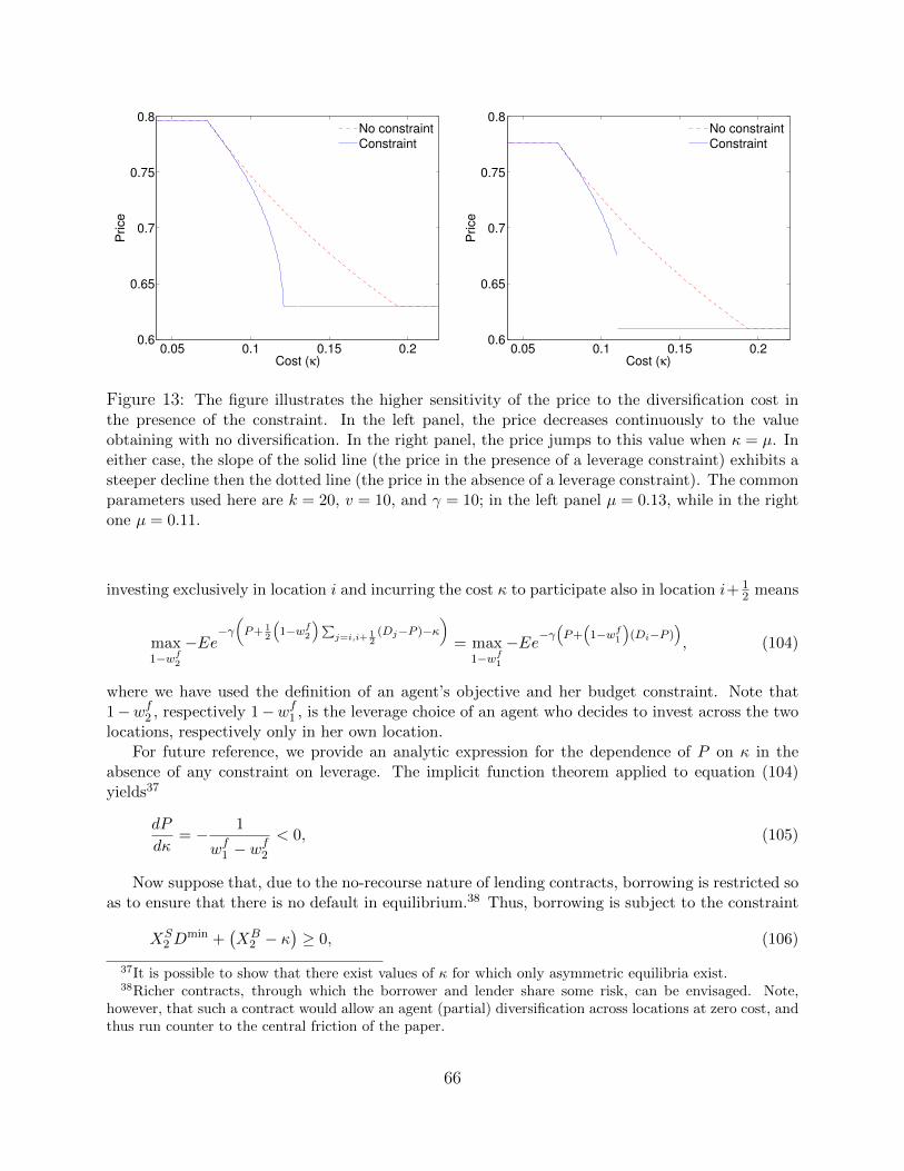
0.05 0.1 0.15 0.20.6

0.65

0.7

0.75

0.8

Cost (κ)

Price

No constraint

Constraint

0.05 0.1 0.15 0.20.6

0.65

0.7

0.75

0.8

Cost (κ)

Price

No constraint

Constraint

Figure 13: The figure illustrates the higher sensitivity of the price to the diversification cost inthe presence of the constraint. In the left panel, the price decreases continuously to the valueobtaining with no diversification. In the right panel, the price jumps to this value when κ = µ. Ineither case, the slope of the solid line (the price in the presence of a leverage constraint) exhibits asteeper decline then the dotted line (the price in the absence of a leverage constraint). The commonparameters used here are k = 20, v = 10, and γ = 10; in the left panel µ = 0.13, while in the rightone µ = 0.11.

investing exclusively in location i and incurring the cost κ to participate also in location i+ 12 means

max1−wf2

−Ee−γ(P+ 1

2

(1−wf2

)∑j=i,i+ 1

2(Dj−P )−κ

)= max

1−wf1−Ee−γ

(P+(

1−wf1)

(Di−P )), (104)

where we have used the definition of an agent’s objective and her budget constraint. Note that1−wf2 , respectively 1−wf1 , is the leverage choice of an agent who decides to invest across the twolocations, respectively only in her own location.

For future reference, we provide an analytic expression for the dependence of P on κ in theabsence of any constraint on leverage. The implicit function theorem applied to equation (104)yields37

dP

dκ= − 1

wf1 − wf2

< 0, (105)

Now suppose that, due to the no-recourse nature of lending contracts, borrowing is restricted soas to ensure that there is no default in equilibrium.38 Thus, borrowing is subject to the constraint

XS2 D

min +(XB

2 − κ)≥ 0, (106)

37It is possible to show that there exist values of κ for which only asymmetric equilibria exist.38Richer contracts, through which the borrower and lender share some risk, can be envisaged. Note,

however, that such a contract would allow an agent (partial) diversification across locations at zero cost, andthus run counter to the central friction of the paper.

66

where Dmin is the smallest possible dividend in period 1, XS2 is the number of shares chosen by

investor a, and −XB2 is the amount borrowed by the investor. Using the time-zero budget constraint

and noting that Dmin = µ and XS2 − 1 = −wf2 , equation (106) becomes

−wf2 (P − µ) ≤ µ− κ. (107)

Attaching a Lagrange λ to the constraint (107) we obtain

dP

dκ= − 1 + λ

wf2 − (1 + λ)wf1< − 1

wf2 − wf1

< 0. (108)

Equation (108) shows an amplification effect: In the presence of the constraint small changes inκ translate into larger drops in the price than would obtain in its absence. This stronger reactionof the price in the presence of the constraint is illustrated in Figure 13, and is analogous to Figure8, where the constraint is modeled as a collateral constraint. The intuition for the increased pricesensitivity, captured by (108), is quite immediate: An increase in κ not only requires the price todecrease in order to avoid a decrease in V2 relative to V1 (the effect behind equation (105)); it alsopushes the price down to counteract the direct effect of tightening of the constraint.

Depending on the parameters, the price may even drop discontinuously to the value obtainingin the no-diversification equilibrium. The point is made most starkly in the case κ = 0 and µ = 0.At these values there is diversification, and no leverage. Any increase in κ, on the other hand, drivesthe price discontinuously down to the no-diversification value. More generally, it can happen that,as κ approaches µ, enough agents continue to diversify — even if their leverage is virtually zero —for the price to be above the no-diversification value that obtains when κ > µ. However, once κexceeds µ the price drops discontinuously, as the right panel of Figure 13 illustrates. Thus, as inSection 5, a small change in κ can cause the nature of the equilibrium to change, which induces adiscontinuous change in the price.

To conclude, even if one modeled borrowing limitations as resulting from a no-default require-ment, the price function is steeper in κ than when the constraint is absent, and can even bediscontinuous, similar to section 5, where the constraint is modeled as a simple leverage constraint.

67