Financial Engineering-Introduction

Financial Engineering• Trading Perspective

– Create structured securities from basic assets to catch specific market niches

• Modeling Perspective– Develop/apply contingent claim valuation

methods to price exotic structured securities• Management Perspective

– Assess the uncertainty of future payoff of portfolio

– Determine strategies to restructure the portfolio risk-return to meet investor’s objectives

Modeling Perspective• Cash flow allocation• Discounted cash flows

– Discount expected cash flows by a Risk-Adjusted Return

– Discount risk-adjusted cash flows by risk-free

t t

t

k

CFEP

1

)(

t t

t

r

CFEP

1

)('

Equilibrium (Risk-adjusted Return) Approach

• CAPM

• APT/Multi-factor CAPM

)( fmf rrrk

....)()( 2211 fff rrrrrk

Equilibrium Approach• Stock value can up to $200 with 70%

probability and down to $50 with 30% probability when risk-free rate is 10%

• Expected payoff = .7 (200) + .3 (50) = $155 – u = 200/100 = 2– d = 50/100 = 0.5– r = 1.10

• Risk-adjusted return = 155/100 - 1 = 55%

• Risk premium = 55% - 10% = 45%

Equilibrium Approach• A call option with exercise price = $125• Possible payoffs are $80 with 70%

probability and $0 with 30% probability• Expected payoff of option = .7 (80) + .3

(0) = $56• Beta of the option = b(C) = 1.83• Risk-adjusted return = k(C) = 10% +

1.83 (45%) = 92.5%• Option Value = C = 56/(1.925) = $29.09

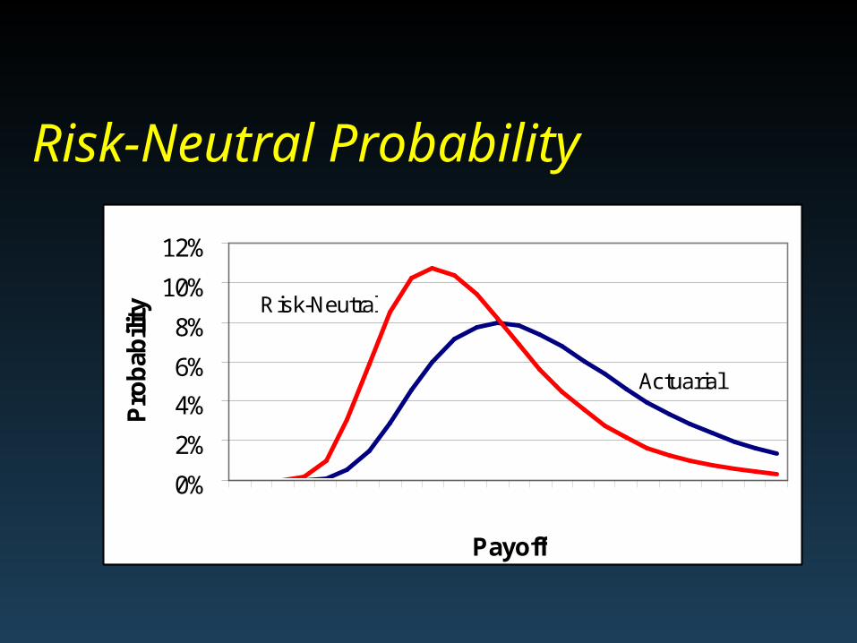
Risk-Neutral Probability

0%

2%

4%

6%

8%

10%

12%1 4 7 10 13 16 19 22 25

Payoff

Probability

Actuarial

Risk-Neutral

Risk-Neutral Approach

• Risk-adjusted probability• Pseudo probabilities

• Discount risk-adjusted expected cash flows at risk-free rate

duru

d

dudr

u

p

p

Risk-Neutral Approach• Risk-neutral probability (u) = =

0.4

• Risk-neutral expected payoff of stock= .4 (200) + .6 (50) = $110

• Stock price = 110/1.10 = $100

• Risk-neutral expected payoff of the call option = .4 (80) + .6 (0) = $32

• Option value = $32/1.10 = $29.09

dudr

Model Solutions• Closed form solutions

– Black-Scholes model, Vasicek model• Finite Difference Methods

– Implicit– Explicit (trinomial tree)– Binomial tree

• Monte Carlo Simulation– Risk-neutral process– Actuarial based process

Examples

• Lattice Method (Binomial Tree)– American Put Option

• Monte Carlo Simulation– Bond pricing under the Hull-White

term structure model

– Value-at-Risk by Bootstrapping

dzdtrdr ttt )(

Closed Form Solutions

• Pros– Fast– Easy to implement

• Cons– Can only work under limited

simplified assumptions, which may not satisfy trading needs

– May not exist for all derivative contracts

Finite Difference Methods• Pros

– Intuitively simple– Fast– Capture forward looking behavior, best for

American style contracts– Accuracy increases with density of time

interval• Cons

– Can not price path-dependent contracts– Difficult to implement, especially with time

and state dependent processes

Monte Carlo Simulations• Pros

– Intuitive– Easy to implement– Matches VaR concept– Accuracy increases with number of

simulations• Cons

– Forwardly simulate cash flows, cannot handle American style contracts

– Slow in convergence

Combined Approaches

• To handle both path-dependent and American style cash flows

• Difficult to implement and time consuming

• Alternative methods– Simulation through tree– Bundled simulation

Management Perspective• Fundamental driving force of financial

engineering• Analyze the risk and return tradeoff for

different cash flow components of an asset/portfolio

• Determine the optimal risk-return profile for the portfolio based on investor’s objectives and constraints– To hedge or not to hedge?

• Value-at-Risk applications• Capital adequacy requirements for: regulator,

rating agency, stock holders

• Financial engineering is the popular name for constructing asset portfolios that have precise technical characteristics– Can construct a put by combining

a short position in the underlying asset with a long call

– Synthetic puts were the first widespread use of financial engineering

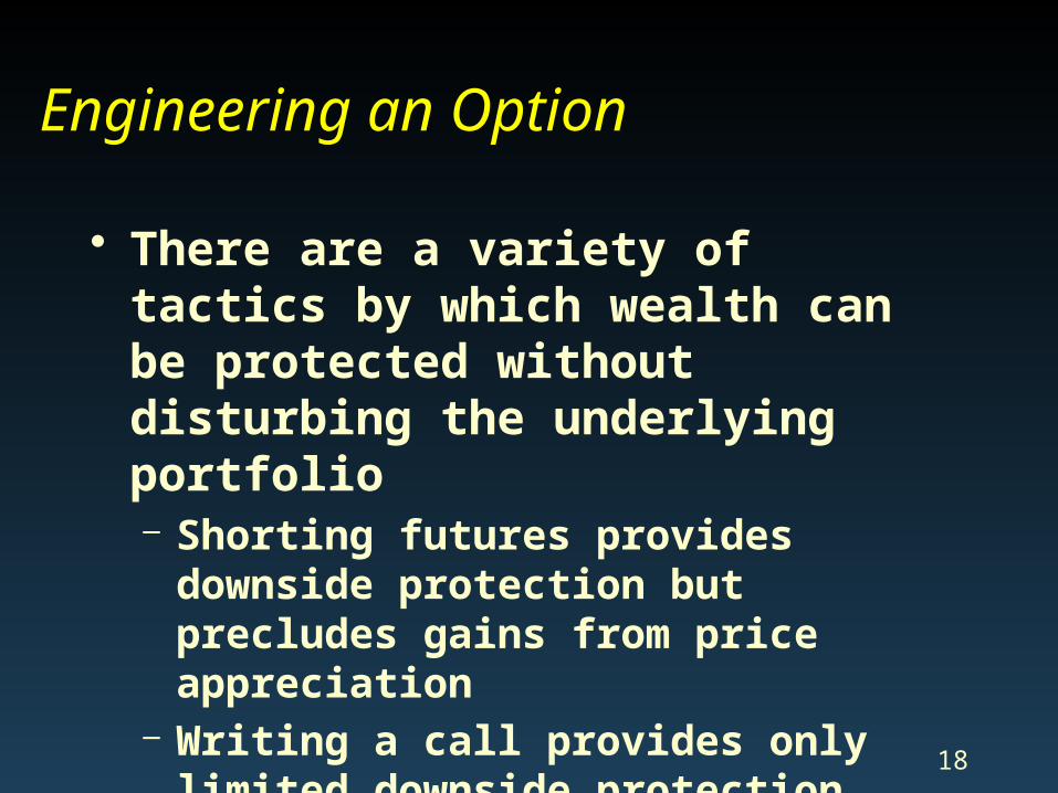
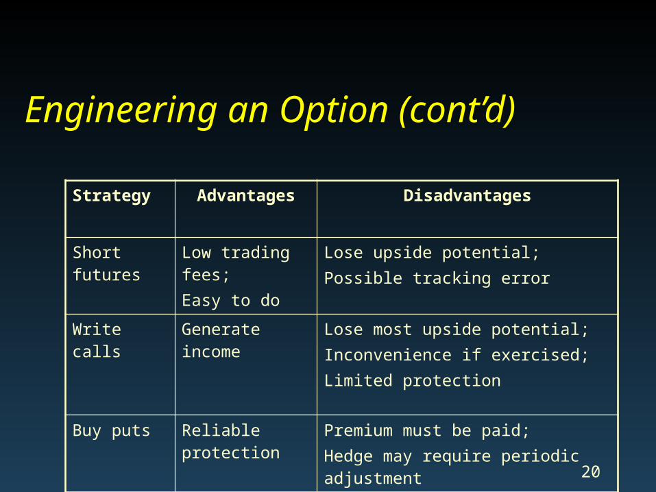
Engineering an Option

• There are a variety of tactics by which wealth can be protected without disturbing the underlying portfolio– Shorting futures provides

downside protection but precludes gains from price appreciation

– Writing a call provides only limited downside protection

– Buying a put may be the best alternative

Engineering an Option (cont’d)

Financial Engineering Example

Assume that T-bills yield 8% and market volatility is 15%. Black’s options pricing model predicts the theoretical variables for a 2-year XPS futures put option with a 325.00 striking price as follows:

Striking price = 325.00Index level = 326.00Option premium = $23.15Delta = -0.388Theta = -0.011Gamma = 0.016Vega = 1.566

Engineering an Option (cont’d)

Strategy Advantages Disadvantages

Short futures Low trading fees;Easy to do

Lose upside potential;Possible tracking error

Write calls Generate income Lose most upside potential;Inconvenience if exercised;Limited protection

Buy puts Reliable protection

Premium must be paid;Hedge may require periodic adjustment

Engineering an Option (cont’d)

Financial Engineering Example

Linear programming models can be utilized to obtain the desired theoretical values from existing call and put options. The greater the range of striking prices and expirations from which to choose, the easier the task.

Primbs, MS&E345 22

What is financial engineering?

Financial Engineering: Combining or carving up existing instruments to create new financial products. (Campbell R. Harvey’s Hypertextual Financial

Glossary, http://www.duke.edu/~charvey/Classes/wpg/glossary.htm)

Another Definition: (from Neil D. Pearson, Assoc. Prof. UIUC)

Definition 1: Financial engineering is the application of mathematical tools commonly used in physics and engineering to financial problems, especially the pricing and hedging of derivative instruments.

Definition 2: Financial engineering is the use of financial instruments such as forwards, futures, swaps, options, and related products to restructure or rearrange cash flows in order to achieve particular financial goals, particularly the management of financial risk.