Financial Choice in a Non-Ricardian Model of Trade∗

Katheryn N. Russ †

University of California, DavisDiego Valderrama ‡

Federal Reserve Bank of San Francisco

November 2009

AbstractWe join the new trade theory with a model of choice between bank and bond financing to

show the differential effects of financial policy on the distribution of firm size, welfare, aggregateoutput, gains from trade, and the real exchange rate in a small open economy. Increasing bankefficiency and reducing bond transaction costs both increase welfare but have opposite effectson the extensive margin of trade, aggregate exports, and the real exchange rate. Increasing thedegree of trade openness increases firms’ relative demand for bond versus bank financing. Weidentify a financial switching channel for gains from trade where increasing access to exportmarkets allows firms to overcome high fixed costs of bond issuance to secure a lower marginalcost of capital.

1 Introduction

The question of how trade openness and domestic financial development interact—and how much

they interact—is an important one, as domestic financial development and trade openness are

favorite policy prescriptions for developing countries.1 Modern trade theory teaches that the gains

from trade depend critically on a reallocation of production from small to large firms. The theory

and empirics of financial development similarly demonstrate that bond market development impacts∗The authors thank Joshua Aizenman, Paul Bergin, Yu-Chin Chen, Silvio Contessi, Galina Hale, Bart Hobijn,

Phillip McCalman, Mark Spiegel, and especially Martin Bodenstein for helpful discussions. Hirotaka Miura providedexcellent research assistance. In addition, we are grateful to the participants at the 2009 APEAMeetings and seminarsat the IMF Institute, Board of Governors of the Federal Reserve, Federal Reserve Bank of St. Louis, Federal ReserveBank of San Francisco, University of California, Santa Cruz, and the University of Washington. The views expressedherein are those of the authors and do not necessarily reflect those of the Federal Reserve Bank of San Francisco orthe Federal Reserve System.

†Department of Economics, One Shields Avenue, Davis, CA 95616, USA. Email: knruss@ucdavis.edu.‡Economic Research, 101 Market Street, MS 1130, San Francisco, CA 94105, USA. Telephone: +1 (415) 974-3225.

Facsimile: +1 (415) 974-2168. Email: Diego.Valderrama@sf.frb.org.1Following the rash of crises in emerging markets in the late 1990s, concerted policy efforts aiming to reduce

dependence on foreign lending and bank financing in favor of domestic bond issues gained momentum among smallopen economies (World Bank and International Monetary Fund, 2001), most notably in the form of the Asian BondMarket Initiative. Greenspan (1999) discuss the potential benefits of developing the domestic bond market as a“spare tire” when foreign financing dries up and banks are undercapitalized. Hong Kong Monetary Authority (2001)discusses how domestic bond markets help “complete” domestic credit markets, improving risk sharing and hedgingby domestic agents.

1

firms differently according to their size. Yet the way that trade policy and specific policies aimed

at credit market development interact through the reallocation of production across heterogeneous

firms who can choose between financial instruments remains unexplored, with unknown implications

for country welfare.

By explicitly modeling features of two different types of financial intermediaries in a model of a

small open economy with heterogeneous firms, we are able to quantify the implications of financial

development on firm behavior and aggregate outcomes. Existing trade models take firm choice

regarding financial instruments to be exogenously determined (allowing firms to borrow in only one

type of credit market) or abstract from financial frictions altogether. Previous studies analyzing

how combinations of financial market imperfections impact different types of firms generally ignore

their interaction with the open economy. We show that policymakers must take into account the

joint effects of trade and intra-industry reallocation when evaluating the merits of policies aimed

at developing specific financial markets and identify a financial switching channel that generates

gains from trade openness.

In our model with financial choice, policies aimed at developing the bond market have quanti-

tatively different implications for economic activity than policies aimed at developing the banking

sector because, ultimately, they each reallocate production across firms in a unique way. Both types

of policies have similar effects along certain dimensions—each increases the average capital-to-labor

ratio, aggregate output, and country welfare. However, they have opposite effects on the extensive

margin of trade, aggregate exports, and the real exchange rate. Further, we show that an increase

in the degree of trade openness by itself can increase firms’ relative demand for bond versus bank

financing, even with no change in the level of transaction costs in the two credit markets. This

result corresponds to the stylized fact shown in Figure 1. The figure shows the growth of the ratio

of domestic corporate bond issuance to domestic bank credit. Countries where exports increase

compared to levels 13 or more years prior also experience growth in domestic corporate bond issues

relative to domestic bank credit over the same period. In contrast, countries where exports decline

experience a drop in the relative size of the bond market. In short, over long horizons countries

with trend growth in exports have trend growth in the prevalence of bond issues as a source of

domestic credit. 2

2Specifically, we split the sample based on whether aggregate exports for each country for each year between 2002

2

The results from our small open economy framework rest on three standard assumptions from

the trade and finance literature. First, we assume that there is an endogenous number of hetero-

geneous, monopolistically competitive firms, as in Melitz (2003) and Ghironi and Melitz (2005).

Firms combine labor and physical capital using a Cobb-Douglas technology to produce varieties

of an intermediate good. Some of the firms export a portion of their output in a world market of

exogenous size. Firms set prices for their unique variety based on their efficiency levels, but these

individual prices have no impact on the composite world price for the intermediate good or on the

aggregate price level in foreign countries. To focus on the role of firm behavior, we abstract from

net capital flow considerations by assuming balanced trade in each period.

Second, we assume that these firms must borrow to finance any investment in physical capital.

This borrowing prompts the third assumption: the existence of what we call financial choice. Firms

can choose between bank and bond financing for their capital expenditures. We model these two

credit instruments very simply as “monitored” versus “unmonitored” lending, in the tradition of

the classic finance literature recently discussed in Freixas and Rochet (1997) and Baliga and Polak

(2004) as well as the modern macroeconomics literature involving costly state verification, discussed

in Carlstrom and Fuerst (1997) and De Fiore and Uhlig (2005). Unmonitored lending is harder to

access than monitored lending but involves a lower interest rate. Thus, in our model, the fixed cost

of issuing public debt (bonds) is much larger than the fixed cost involved in securing a loan.

The fixed cost of bond issuance is used to make a firm’s balance sheet transparent to investors

and reduces the monitoring cost. It can represent the fees charged for underwriting and commis-

sions by investment banks that study the value of a firm’s liquid assets then use their networks

and expertise to inform potential bond investors so that they more easily can recover their full

investment if a bond issuer defaults, though without interest. Alternatively, it can represent an

insurance fee guaranteeing that investors will fully recover all assets in the event that a firm de-

faults. The key is that the fee reduces or eliminates monitoring costs for bond investors. Endo

(2008) and Burger and Warnock (2006) find that policy actions influencing costs of domestic bond

and 2008 have increased or decreased relative to 13, 14, ..., or 19 years before. Then we indicate on the vertical axisthe log difference in the ratio of domestic corporate bond issues to domestic bank claims during the same period (overthe previous 13, 14, ..., or 19 years), averaging over observations in each half of the split sample. Data for exportsand domestic bank claims on the private sector are from the International Monetary Fund International FinancialStatistics. Data for domestic corporate (nonfinancial) bond issues are from the Bank for International Settlementsonline historical series. We use all countries for which there is data in all three series, for a total of 39 countries.

3

issuance—including both direct regulatory fees and costs induced by regulatory uncertainty re-

garding whether and when an issuance can take place—are important determinants of the level of

domestic bond market development. Accordingly, we choose to embody the policy stance regarding

bond market development within this fixed cost.3 The smaller fixed cost of monitored bank lending

makes it more easily accessible to smaller firms. Easier access comes with a higher marginal cost

of financing capital, as banks must closely monitor borrowers who default, passing this higher cost

on to all bank borrowers in the form of higher interest rates. In our model, this combination of

financial frictions results in less efficient small firms being dependent on bank credit, while larger,

more efficient firms are able to exploit the lower marginal costs of financing in the bond market.4

Policies that reduce the fixed cost of bond issuance induce firms to switch from bank borrowing

to bond issuing as a source of credit, thus decreasing their marginal cost of capital since interest

paid on bonds is lower than interest paid on bank loans. These switchers reduce their prices5

to capture additional domestic and external market share, which lowers the aggregate domestic

price level. If these switchers were exporters before the regime change, they can export more after

switching to bond purchases due to their new lower prices. Ironically, even though switchers expand

their production for the domestic and overseas markets, the extensive margin shrinks for both

domestic production and trade. The increased competitiveness of switchers relative to nonswitchers,

combined with an increase in the real wage, owing to the combined effects of the increased demand

for labor and the falling aggregate price level, pushes the very least efficient nonswitchers out of

business and the least efficient nonswitching exporters out of the export market. Aggregate exports

also fall. The exit of the least productive domestic producers drives the aggregate price level down

a bit more than just the reduction in prices among switchers. Through its dampening effect on

the domestic price level, bond market development causes the real exchange rate to depreciate.

Policies that increase the efficiency of the banking sector through measures that lower monitoring

costs have a very different reallocative effect than lowering the fixed cost of bond issuance. These

policies reduce the interest rates that banks charge and therefore lower marginal costs for all firms3One might also usefully consider the overall liquidity and maturities of the issues within a bond market that

impact bond yields. However, the number of participants in the bond market influence the liquidity and variety ofissues and fixed costs involved in issuing bonds certainly impact the number of participants (buyers as well as issuers).We focus on the fixed cost of issuance as a first step in defining and analyzing financial choice.

4See Russ and Valderrama (2009) for a survey of the theory and evidence surrounding bank and bond financingthat produced this stylized fact regarding sources of financing for small versus large firms.

5Prices are a constant markup over marginal cost in our monopolistically competitive framework.

4

that rely on bank loans, not just for the subset of firms that switch financing sources. These

bank-dependent firms lower prices and increase output. Falling interest rates on bank loans induce

the marginal bond issuers to switch to bank financing. The switch reduces their fixed cost but

increases their marginal cost, causing switching firms to raise their prices and lower their output.

Additionally, lowering the marginal cost of bank financing induces more firms to produce for both

the domestic and export markets. These additional participants are less productive than incumbent

producers and exporters. Their reduced efficiency, in combination with the price increases among

switchers, outweighs the effect of lower bank lending costs on the aggregate price level. As a result

the aggregate price level rises, causing the real exchange rate to appreciate. At the same time, the

expanded extensive margin of trade contributes to an overall increase in aggregate exports.

Considering an open economy model with endogenous financial choice and heterogeneous firms

allows us to study the impact of exogenous changes in iceberg trade costs on measures of finan-

cial development in a brand new way. An change in the iceberg cost might be caused by tariff

reductions; special export processing zones; or improved access to transport through investments

in infrastructure, technological growth or increased competition in transport industries. A reduc-

tion in an iceberg trade cost causes a reallocation of production away from most incumbent firms

toward a small subset of new entrants, firms that begin to export, and exporters who switch from

bank loans to bonds because they find the lower iceberg cost increases variable profits and allows

them to pay the fixed cost of bond issuance. Further, we identify this phenomenon as a financial

switching channel for gains from trade where increasing access to export markets allows firms to

overcome high fixed costs of bond issuance to secure a lower marginal cost of capital; this channel

grows stronger when issuance costs are low.

Given our balanced trade assumption, the increase in aggregate exports means more imports,

which are all intermediate goods by assumption. The increase in imported intermediates generates

a complementarity in the assembly of final goods: demand increases for domestic varieties so that

some new firms start to produce for the domestic market. These new firms are the smallest in the

economy and use bank credit. The new bank-borrowing exporters are also small in comparison

to the largest bank borrowers who suddenly switch to bond issues. Thus, reducing variable trade

costs increases the ratio of bond issues to bank credit. What is more, the sectoral reallocation

of production from the largest firms to smaller firms causes a real exchange rate appreciation as

5

production shifts to firms with higher marginal costs (given their low efficiency) and thus higher

prices.

A reduction in the fixed cost of exporting has quite different effects on financial choice and

on the relative size of different financial markets. Reducing fixed barriers to export participation

allows more bank borrowers to become exporters. Because the increase in production for export

sale occurs only at the smaller end of the firm size distribution, there is less impact on prices and the

real wage. The number of large exporting bond issuers falls just a bit due to the general equilibrium

wage effect, so that aggregate exports are relatively stable. There is no complementary boost in

the demand for domestic varieties to combat the second-order wage effect, so the smallest firms are

forced to exit. In this case, the expansion of new exporters among bank borrowers outweighs exit

at the bottom end of the size spectrum. Thus, the level of bank credit increases dramatically in

comparison to the stable level of bond issues, completely opposite to the effect of lowering variable

trade costs.

The following section discusses existing studies on the implications of different types of financial

frictions for exporting behavior, as well as the fledgling literature examining the choice of financing

instruments among firms in an open economy. Sections 3 and 4 describe the conversion of house-

hold savings into capital expenditures, as well as firm-level decisions about whether to finance

them using bank loans or bond issues and whether to export. Section 5 describes the steady-state

equilibrium and discusses the calibration of the model. Section 6 discusses the results of various nu-

merical exercises illustrating the relationship between financial market development, intra-industry

reallocation, the extensive margin of trade, gains from trade liberalization, and the real exchange

rate. We conclude in Section 7 with suggestions for further research.

2 Related literature

Relating the tradeoffs between banking sector and bond market development with trade flows in a

heterogeneous firm framework crosses several segments of literature. There is a deep foundation of

theoretical and empirical work analyzing the choice between banks and bonds in the closed economy,

which several sources survey in detail (Freixas and Rochet, 1997; De Fiore and Uhlig, 2005; Russ and

Valderrama, 2009). However, our motivating question—How does financial choice impact welfare in

6

an open economy?—arises from piecing together a diverse patchwork of studies relating individual

financial frictions to the pattern of trade and another very small but growing branch of literature

focusing on the impacts of firms’ choice between sources of financing on macroeconomic outcomes

in open economies. We briefly describe the two approaches and how our work ties them together.

2.1 Financial frictions and trade

While we examine the impact of transaction costs and monitoring costs in credit markets on financ-

ing choice, intra-industry reallocation of production, and export decisions in a small open economy,

previous studies in international trade and macroeconomics characterize financial frictions in the

form of explicit credit constraints. These papers are extremely innovative and important because

they rigorously characterize a link between financial development and export behavior in an empir-

ically relevant way. At the same time, they abstract from financial choice: the lack of access to full

financing is exogenously given rather than an endogenous outcome arising from transaction costs,

and firms must borrow from one particular source, by assumption.

Chaney (2005) and Manova (2008) consider the impact of credit constraints on intra-industry

reallocation and export decisions in models with heterogeneous firms. Chaney (2005) supposes

that firms can borrow to finance fixed costs of domestic production but must generate their own

liquidity—defined as domestic profits plus an exogenous endowment of fungible assets—to pay fixed

costs of exporting due to incompleteness in credit markets. Some firms that could profitably export

do not because they lack liquidity to enter the overseas market. The study explicitly leaves the

exploration of specific vehicles for financing domestic investment open for future research, focusing

instead on the interaction between the liquidity constraint and macroeconomic shocks to observe

the relationship between the extensive margin of trade and the real exchange rate. Credit con-

straints distort the entry and exit of exporters, offering a brand new explanation for incomplete

pass-through. In our model, we focus instead on basic features of two specific types of financial in-

termediaries to examine the interaction of trade and financial policy on the allocation of production

across firms. While we do not look at short-term fluctuations arising from macroeconomic shocks,

we show that small open economies experience a real depreciation if they develop their bond market

by reducing issuance costs or if they subsidize bank credit or experience a real appreciation if they

increase the efficiency of their banking sector in ways that reduce spread between the interests rate

7

on loans and bonds. In our model, the changes in the real exchange rate occur as an endogenous

outcome.

Manova (2008) assumes that heterogeneous firms must borrow to finance both fixed and variable

trade costs, varying the fraction of trade costs that must be externally financed by industry. Manova

enriches the model by introducing collateral, exogenously varying the degree to which externally

financed purchases can be used as collateral by industry and the probability of default. In this

context, the model is able to explain observed industry-level trade flows between countries with

different levels of financial development. In contrast, our model involves only one industry but

incorporates physical capital. We assume that all firms must finance all capital expenditures in

advance using external credit, but all labor and trade costs out of cash revenues at the time of sale.

All firms have, in principle, access to both types of financing, bonds and loans. However, depending

on the firm-specific efficiency level, each firm chooses to finance either through bank loans or by

issuing bonds. The degree to which capital expenditures serve as collateral varies by the type of

financial intermediary, rather than by industry. In bond markets, a large issuance cost is used to

broadcast information about the firm that reduces or eliminates monitoring costs for bondholders

when firms default, allowing them to recoup borrowed capital with little or no loss of principal.

Banks, on the other hand, must go through costly proceedings to audit and press the fraction of

firms that default for repayment, burning up a larger fraction of borrowers’ collateralized capital

holdings in the form of monitoring costs. Firms that choose to finance through bank loans pay this

cost in the form of higher interest rates, resulting in higher marginal costs of capital that make

them less able to export. Our aim is to contrast the impact of altering the relative attractiveness of

these two different types of financial instruments on aggregate outcomes in a small open economy.

In addition to the contributions of Chaney (2005) and Manova (2008), a rich literature holds

that there is a recursive relationship between comparative advantage and domestic financial devel-

opment. Antràs and Caballero (2009) introduce financial frictions in a Heckscher-Ohlin/Mundell-

Vanek framework to show that, in financially underdeveloped countries, trade and capital flows

can be complements rather than substitutes, in contrast to the traditional capital-flows approach

established by Mundell (1957).6 The authors allow for capital mobility across countries and also6Antràs and Caballero (2009) note a new generation of theoretical contributions beginning with the seminal work

of Bardhan and Kletzer (1987), with the most recent empirical support for the link between financial development andcomparative advantage provided by Manova (2008). We refer the reader to their comprehensive survey of financial

8

model financial frictions as an exogenous credit constraint—a refusal on the part of intermedi-

aries to lend quite as much to producers as they need to purchase the optimal level of capital for

production. The degree of financial development influences the degree of comparative advantage

and trade patterns. We abstract from international capital flows in our model to focus on the

structure of specific domestic financial institutions—banks and bond markets—showing that they

have different effects on the capital-to-labor ratio (the driving source of comparative advantage in

Ricardian models), welfare, and the extensive margin of trade.

In a contrasting approach, Do and Levchenko (2007) suggest that the degree of comparative

advantage and pattern of trade can influence a country’s level of financial development, rather than

viceversa. They provide empirical evidence that specialization in industries requiring more external

finance promotes more developed financial markets. Our model captures their finding that that

trade flows can drive financial development, measured by the ratio of total private credit to gross

domestic product (GDP).

2.2 Firm financing decisions in the open (macro) economy

Razin and Sadka (2007) and Smith and Valderrama (2009) are two recent theoretical contributions

that analyze the macroeconomic consequences of financing choice in an open economy setting.

Both of these papers focus on the impact that financing choice has on macroeconomic outcomes,

particularly on the composition of aggregate capital flows.7 Razin and Sadka (2007) consider the

impact of two forms of firm financing for capital investment, foreign direct investment (FDI) and

portfolio investment, on aggregate capital flows while allowing for firm heterogeneity. The key

mechanism of their model lies in sensitivity of heterogeneous investors, who make the key financial

choices, to liquidity shocks. Countries with greater macroeconomic volatility attract investors who

are less sensitive to liquidity shocks and attract less-reversible FDI, while countries that are more

prone to liquidity shocks attract investors who prefer more-reversible portfolio investment. FDI

reveals more information about the firm, so that firms that attract FDI optimally adjustment

their capital stock and grow more. Thus, financial choice by investors has important consequences

for the aggregate capital stock, as well as the overall balance of FDI and portfolio flows in a

frictions and comparative advantage.7See Russ (2009) for a discussion of the split between the study of firm financing decisions (with a focus on foreign

direct investment) and the study of trade and capital flows.

9

country’s financial account. We consider financial choice from the perspective of the firm and the

intermediary, rather than the investor. The gap is fertile ground for future research.8

Smith and Valderrama (2009) use a structural model to show that the choice of financing (by

selling the firm via FDI, issuing additional equity shares, or borrow using bonds) by a representative

firm can influence the properties of the real business cycle in small open economies. In contrast

to Razin and Sadka (2007) and Smith and Valderrama (2009), we do not study the role that firm

financing decisions have on capital flows. We focus instead on the role that domestic financial im-

perfections have on the steady-state level of financial development, production reallocation, export

decisions, and the real exchange rate. Most firms in emerging markets do not have access to foreign

capital markets, so we view our focus on domestic financial institutions as the most relevant to

study the impact of financial frictions across the entire spectrum of firms operating in an economy.

Levchenko, Rancière, and Thoenig (2009) provide empirical evidence using industry-level data

that increased access to credit following financial liberalization increases firm entry, employment,

and capital investment, leading to a positive aggregate growth effect. However, due to data con-

straints it is not clear exactly which features of the institutional change are driving the change in firm

behavior, or if different types of financial development impact firm behavior differently. Our model

can rationalize some of the findings in Levchenko, Rancière, and Thoenig (2009) while establishing

causal relationships between a reduction in financial frictions and endogenous outcomes—intra-

industry reallocation; firm decisions regarding entry, investment, and employment; and aggregate

output.

3 Savings and investment

In the model introduced here, savings by consumers are transformed into funds for capital through

two forms of domestic financial intermediaries, banks and bond underwriters. The emphasis of

the study is on the impact of financial imperfections on the decisions by firms about borrowing,

production, and export decisions and macroeconomic aggregates. Households provide important

inputs to production through their supply of inputs to firms via savings and labor, and their

consumption and welfare are determined endogenously. This section describes the problem of8For instance, see Fillat and Garreto (2009) for empirical evidence relating fluctuations in equity values to firms’

decisions to invest in global markets as multinationals versus domestically as exporters.

10

the representative household and financial intermediaries, while Section 4 describes the financial,

production, and export decisions by firms.

3.1 Households

The representative consumer maximizes lifetime utility,

maxCt,Lt,KS

t+1

∞∑t=0

βtU(Ct, Lt),

where

U(Ct, Lt) = 11− η

(Ct −

Lψtψ

)1−η

,

and Ct and Lt represent aggregate consumption and the labor supply in period t.

The consumer maximizes utility subject to an intertemporal budget constraint,

PtYt = PtCt + PtKt+1 = wtLt + rtPtKt + (1− γ)PtKt + πIt + πFt , (3.1)

with Pt being the aggregate price level and πFt and πIt representing firm profits and fees charged

by financial intermediaries which are paid back in the form of dividends to the consumer. Units of

aggregate output, Yt, can be devoted either to consumption or to savings. The term Kt+1 denotes

consumer savings from period t income transformed into capital expenditures for use in period t+1.

The representative consumer receives a return of rt on each unit of capital set aside for the next

period, regardless of whether the savings are in the form of bank deposits or corporate bonds.9

Capital depreciates at rate γ.

In steady state, the relevant results from the consumer’s first-order conditions are equations

that determine the labor supply as a function of the real wage rate alone and the gross rate of9We will explain below that the risk-adjusted return on both assets must be equal to eliminate any arbitrage

opportunity. We assume that bond underwriters assume the risk of default on bonds to streamline notation (usingonly one rate of return on savings) in the consumer’s problem, but we could achieve an observationally equivalentsteady-state result by transferring the risk to consumers and specifying a separate rate of return for household bondholdings versus bank deposits, which are riskless. In reality, underwriters conducting a primary issue do assumesignificant risk between the time they purchase bonds from firms and sell them to investors.

11

return on savings being pinned down by the consumer’s discount factor and the depreciation rate:

L =(w

P

)( 1ψ−1

)and (3.2)

1 + r = 1β

+ γ, (3.3)

respectively.

3.2 Financial intermediaries

The corporate finance literature focuses on two salient features when contrasting banks and bond

markets as sources of funds for capital expenditures: large bond issuance costs and high interest

rates on bank loans. A number of authors explain that high bond issuance costs are necessary

to disseminate information regarding firms’ balance sheets to potential investors. Others posit

that special relationships between banks and firms arise to surmount problems of asymmetric

information. Overcoming the asymmetric information problem can lead to higher interest rates on

bank loans for two reasons. It can make it costly for customers to develop a relationship with a

new lender, engendering monopoly power among bank managers. Alternatively, it can force a bank

to “monitor” some borrowers to make sure they repay their loans, even in a perfectly competitive

market for bank credit. These monitoring costs are also referred to as “costly state verification”—if

a borrower defaults, a bank incurs costs to audit the borrower, sue, or liquidate the borrower’s

assets to recover accounts payable. We assume that large issuance costs make the monitoring cost

lower for bondholders than for banks.

We incorporate these two features in the simplest way possible to focus on the intuition behind

the impacts the two types of financing can have on firm behavior in an open economy. To finance

capital expenditures using bonds, a firm must pay a large fixed cost, f̃b = (1 + rb)fb.10 We assume

that this fixed cost makes the firm transparent to investors from the time of issue, with little or no

monitoring necessary. It is sufficient that the monitoring cost for bonds merely be lower than that

for bank loans. Without loss of generality, we assume it is zero for simplicity. In our stylized setup,10We assume that creditors "front" borrowers this fixed cost, f̃b, which is paid with interest at the end of the

period. This corresponds to the practice of underwriters including fees as part of the "gross spread" between the priceat which they purchase bonds from firms and the price at which they sell the bonds to investors. For consistency,we model the fixed cost of bank loans the same way, as though closing costs and other fees are included in the loanprincipal.

12

this “unmonitored” lending means that even if a firm tries to default, bondholders have information

that allows them to costlessly seize and liquidate all of the firm’s capital holdings without any of

the difficulties involved in audits and bankruptcy proceedings faced by banks. The primary risk

posed by default in this case is that they receive no interest on the borrowed capital. Thus, bond

yields rb are equal to the steady-state interest rate shown in equation (3.3), adjusted for the risk

of default: rb = r1−δ .

11 We assume that underwriters assume the entire risk of default between the

time they purchase bond issues from firms and sell them to households to simplify the exposition of

the consumer’s problem, but the result is observationally equivalent in steady state when consumers

bear the risk instead of underwriters, as they will still demand the same risk-adjusted interest rate,

rb.

Obtaining a bank loan incurs a smaller fixed cost than bond issuance: f̃l = (1 + rb)fl, with

f̃l < f̃b. The interest rate banks charge on loans include an extra markup over the deposit rate r to

cover costly state verification for a fraction of firms that try to default. Define δ as the fraction of

firms that receive an exogenous forced exit shock and try to default on their loans.12 The exit shock

does not destroy capital holdings, but makes the firm unable to produce. In our model, it does not

matter if the default rate is lower for bond issuers, as seen in Diamond (1991) and related models,

because it still results in a bond yield that is lower than the interest rate on bank loans. We assume

that δ is equal across firms for simplicity and to align it with existing models of heterogeneous firms

in open economies. Suppose that banks have to pay some fraction, µ, of the total amount of their

loans to defaulting firms in order to recover the firms’ borrowed capital holdings. For simplicity

(and without loss of generality) we assume that the monitoring cost for bondholders is equal to

zero. Then banks must charge an interest rate at least high enough to cover expected monitoring

costs, generating a spread between the interest rates that banks charge on loans, rl, and the bond

yield. If banks are perfectly competitive, then this spread is a function of the monitoring cost and

the default rate:13

rl = rb + δµ

1− δ . (3.4)

11See Appendix A for derivation.12This forced exit shock is drawn from Melitz (2003) and is equal to the net exit rate in steady state. The exit rate

involving plant closings in Dunne, Roberts, and Samuelson (1988) (8.7–17.3 percent for new plants, 1.1–2.2 percentfor established plants) is similar to the default rates surveyed by Russ and Valderrama (2009).

13See Appendix A for derivation.

13

It follows that the marginal costs for firms financing capital expenditures using bank loans will

always be higher than marginal costs for firms financing capital expenditures using bond issues.

4 Firms

In this section we describe the problem faced by firms. Final goods are produced by competitive

firms using both domestically produced and imported intermediate goods. The focus of our study

is on the domestic intermediate goods producers. These producers are imperfectly competitive

and take the wage rate, the interest rate (for bonds or loans), and the fixed costs of financing and

exporting as given. They produce using a constant-returns-to-scale technology. Individual firms

observe their idiosyncratic level of efficiency before making financing, production, and export deci-

sions. In equilibrium, depending on its level of efficiency, each firm elects to produce domestically

if its expected profits are high enough to cover the costs of production and financing. We show

that under a very mild assumption supported by data on interest rates and fixed costs of financing,

the marginal active firm will be a bank borrower, while firms with very high levels of efficiency will

borrow by issuing bonds. This result corresponds with the stylized fact in the finance literature

that bond issuers tend to be larger than bank borrowers.

Firms must pay an additional fixed cost before entering the export market. Thus, it is easy to

show that exporting firms always serve the domestic market, though not all firms that serve the

domestic market also export. Depending on the relative cost of capital, the wage rate, and the

different fixed costs, it is possible that the marginal exporter is a bank borrower or a bond issuer.

Below, we show the conditions under which the marginal exporter is a bank borrower (the case we

consider most plausible) and focus on this case in the numerical exercises. If the marginal exporter

is a bank borrower, then it can be shown that all bond issuers will produce both for the domestic

market and also export.

14

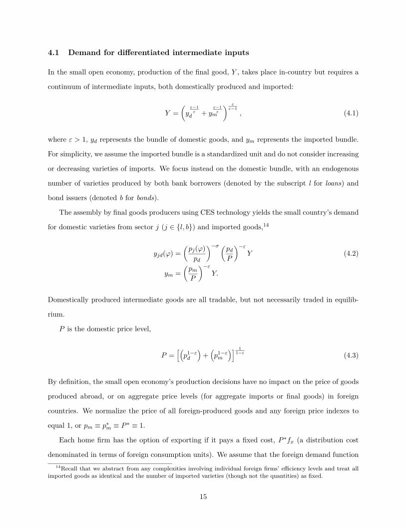
4.1 Demand for differentiated intermediate inputs

In the small open economy, production of the final good, Y , takes place in-country but requires a

continuum of intermediate inputs, both domestically produced and imported:

Y =(yε−1ε

d + yε−1ε

m

) εε−1

, (4.1)

where ε > 1, yd represents the bundle of domestic goods, and ym represents the imported bundle.

For simplicity, we assume the imported bundle is a standardized unit and do not consider increasing

or decreasing varieties of imports. We focus instead on the domestic bundle, with an endogenous

number of varieties produced by both bank borrowers (denoted by the subscript l for loans) and

bond issuers (denoted b for bonds).

The assembly by final goods producers using CES technology yields the small country’s demand

for domestic varieties from sector j (j ∈ {l, b}) and imported goods,14

yjd(ϕ) =(pj(ϕ)pd

)−σ (pdP

)−εY (4.2)

ym =(pmP

)−εY.

Domestically produced intermediate goods are all tradable, but not necessarily traded in equilib-

rium.

P is the domestic price level,

P =[(p1−εd

)+(p1−εm

)] 11−ε (4.3)

By definition, the small open economy’s production decisions have no impact on the price of goods

produced abroad, or on aggregate price levels (for aggregate imports or final goods) in foreign

countries. We normalize the price of all foreign-produced goods and any foreign price indexes to

equal 1, or pm ≡ p∗m ≡ P ∗ ≡ 1.

Each home firm has the option of exporting if it pays a fixed cost, P ∗fx (a distribution cost

denominated in terms of foreign consumption units). We assume that the foreign demand function14Recall that we abstract from any complexities involving individual foreign firms’ efficiency levels and treat all

imported goods as identical and the number of imported varieties (though not the quantities) as fixed.

15

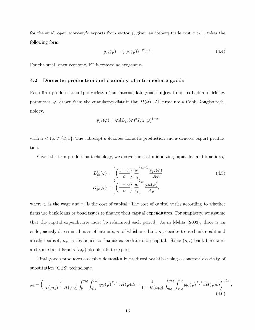
for the small open economy’s exports from sector j, given an iceberg trade cost τ > 1, takes the

following form

yjx(ϕ) = (τpj(ϕ))−σ Y ∗. (4.4)

For the small open economy, Y ∗ is treated as exogenous.

4.2 Domestic production and assembly of intermediate goods

Each firm produces a unique variety of an intermediate good subject to an individual efficiency

parameter, ϕ, drawn from the cumulative distribution H(ϕ). All firms use a Cobb-Douglas tech-

nology,

yjk(ϕ) = ϕALjk(ϕ)αKjk(ϕ)1−α

with α < 1,k ∈ {d, x}. The subscript d denotes domestic production and x denotes export produc-

tion.

Given the firm production technology, we derive the cost-minimizing input demand functions,

L∗jk(ϕ) =[(1− α

α

)w

rj

]α−1yjk(ϕ)Aϕ

(4.5)

K∗jk(ϕ) =[(1− α

α

)w

rj

]αyjk(ϕ)Aϕ

,

where w is the wage and rj is the cost of capital. The cost of capital varies according to whether

firms use bank loans or bond issues to finance their capital expenditures. For simplicity, we assume

that the capital expenditures must be refinanced each period. As in Melitz (2003), there is an

endogenously determined mass of entrants, n, of which a subset, nl, decides to use bank credit and

another subset, nb, issues bonds to finance expenditures on capital. Some (nlx) bank borrowers

and some bond issuers (nbx) also decide to export.

Final goods producers assemble domestically produced varieties using a constant elasticity of

substitution (CES) technology:

yd =( 1H(ϕbd)−H(ϕld)

∫ nld

0

∫ ϕbd

ϕld

yld(ϕ)σ−1σ dH(ϕ)di+ 1

1−H(ϕbd)

∫ nbd

nld

∫ ∞ϕbd

ybd(ϕ)σ−1σ dH(ϕ)di

) σσ−1

,

(4.6)

16

where σ > 1. In this expression, we use the result shown later that bank borrowers have idiosyn-

cratic productivity in the interval [ϕld, ϕbd), and bond issuers have productivity in the interval

[ϕbd,∞).

The price index for the bundle of domestically produced and consumed goods is then

pd = σ

σ − 1wα

(1− α)1−α.ααAϕ̄, (4.7)

The aggregate productivity level for domestically consumed home production, ϕ̄, is defined in terms

of the average productivity level among bank borrowers, ϕ̄ld, and bond issuers, ϕ̄ld, as

ϕ̄ =(nldr

−(1−α)(σ−1)l ϕ̄σ−1

ld + nbdr−(1−α)(σ−1)b ϕ̄σ−1

bd

) 1σ−1 .

The sectoral efficiency levels among bank borrowers and bond issuers are then

ϕ̄σ−1ld ≡ 1

H(ϕbd)−H(ϕld)

∫ ϕbd

ϕld

ϕσ−1dH(ϕ) and (4.8)

ϕ̄σ−1bd ≡ 1

1−H(ϕbd)

∫ ∞ϕbd

ϕσ−1dH(ϕ), (4.9)

respectively.

4.3 The marginal firm

After deciding whether to become active, firms draw their efficiency level and then decide whether

to produce or export. Firms earn profits from domestic sales:

πjd(ϕ) = 1σ

(pj(ϕ)pd

)1−σ (pdP

)1−εPY − P f̃j j ∈ {l, b}.

A firm will not be active at all unless it is at least sufficiently productive to serve the domestic

market without losing money. Thus, there is a participation constraint for domestic production,

πjd(ϕjd) ≡ 0.

It is straightforward to show that this marginal participant will be a bank borrower as long as

17

the gap ratio of the fixed cost of bond issues and bank borrowing is sufficiently large relative to the

ratio of the interest rates associated with bank and bond credit.15 More specifically, the marginal

participant is a bank borrower as long as the following condition holds:

f̃b

f̃l>

(rlrb

)(1−α)(σ−1). (4.10)

The condition requires that the marginal cost advantage of bond financing is large enough that

any firm sufficiently profitable to pay the fixed cost of issuance with do so. Taking the ratio of

the average prime rate and average Moody’s Seasoned Aaa bond yield from January 1949 through

July 2007, this condition requires that the fixed cost of bond issues be only 1–10 percent higher

than the fixed cost of securing bank credit for standard parameterizations of α and σ, well within

the range observed in the data. In our simulations, we assume that this condition holds, so that

profits for the marginal bank borrower are zero:

πld(ϕld) ≡ 0. (4.11)

Equation (4.11) pins down the value of the efficiency level for the marginal bank-borrowing pro-

ducer, ϕld.

4.4 The marginal exporter

If a firm pays an additional fixed export cost, fx, it can earn profit from export sales to the rest of

the world,

πjx(ϕ) = τ−σ

σ(pj(ϕ))1−σ Y ∗ − P f̃x.

Because the firm knows how efficient it is before deciding to export and because exporting requires

an additional fixed cost, any firm that exports also serves the domestic market. Therefore, we

express total profit for the individual firm as

πTj (ϕ) = max [0, πjd(ϕ) + max {0, πjx(ϕ)}]15The sufficient condition for this marginal domestic producer to be a bank borrower requires only that the

domestic profit equation be steeper for a bond issuer than for a bank borrower and that the domestic profit functionsof the two are equal where profits are greater than zero. See Russ and Valderrama (2009) for a detailed discussion.

18

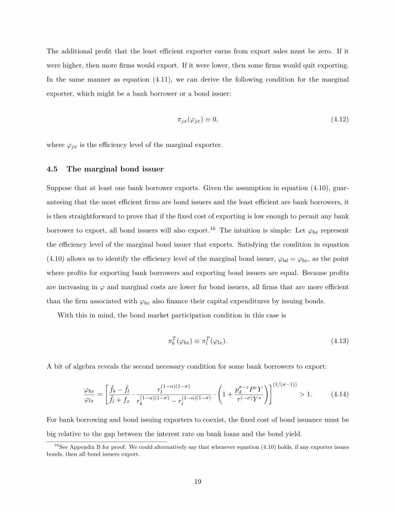
The additional profit that the least efficient exporter earns from export sales must be zero. If it

were higher, then more firms would export. If it were lower, then some firms would quit exporting.

In the same manner as equation (4.11), we can derive the following condition for the marginal

exporter, which might be a bank borrower or a bond issuer:

πjx(ϕjx) ≡ 0, (4.12)

where ϕjx is the efficiency level of the marginal exporter.

4.5 The marginal bond issuer

Suppose that at least one bank borrower exports. Given the assumption in equation (4.10), guar-

anteeing that the most efficient firms are bond issuers and the least efficient are bank borrowers, it

is then straightforward to prove that if the fixed cost of exporting is low enough to permit any bank

borrower to export, all bond issuers will also export.16 The intuition is simple: Let ϕbx represent

the efficiency level of the marginal bond issuer that exports. Satisfying the condition in equation

(4.10) allows us to identify the efficiency level of the marginal bond issuer, ϕbd = ϕbx, as the point

where profits for exporting bank borrowers and exporting bond issuers are equal. Because profits

are increasing in ϕ and marginal costs are lower for bond issuers, all firms that are more efficient

than the firm associated with ϕbx also finance their capital expenditures by issuing bonds.

With this in mind, the bond market participation condition in this case is

πTb (ϕbx) ≡ πTl (ϕlx). (4.13)

A bit of algebra reveals the second necessary condition for some bank borrowers to export:

ϕbxϕlx

=[f̃b − f̃lf̃l + fx

·r

(1−α)(1−σ)l

r(1−α)(1−σ)b − r(1−α)(1−σ)

l

·(

1 + pσ−εd P εY

τ (−σ)Y ∗

)](1/(σ−1))

> 1. (4.14)

For bank borrowing and bond issuing exporters to coexist, the fixed cost of bond issuance must be

big relative to the gap between the interest rate on bank loans and the bond yield.16See Appendix B for proof. We could alternatively say that whenever equation (4.10) holds, if any exporter issues

bonds, then all bond issuers export.

19

Do all firms export? Not necessarily. Dividing the ϕxl by ϕl obtained from equations (4.12)

and (4.11), we derive the efficiency level of the marginal exporter as a function of the efficiency

level of the least productive firm that serves the domestic market:

ϕlx =[(

f̃l + fx

f̃l

)(pσ−εd P εY

τ−σY ∗

)]( 1σ−1 )

ϕld. (4.15)

Nontraded goods exist whenever ϕlx > ϕld. The intuition is clear: there are nontraded goods

whenever the fixed cost of exporting is large enough relative to the fixed cost of securing bank

credit and the degree of domestic absorption is sufficiently high that it is worthwhile to produce

even if a firm cannot export.

If the condition in equation (4.14) does not hold then the marginal exporter is a bond issuer

and we need only solve for ϕld, ϕbd, and ϕbx. In this case, equation (4.15) becomes

ϕbx =[(

rbrl

)(1−α)(f̃b + fx

f̃l

)(pσ−εd P εY

τ−σY ∗

)]( 1σ−1 )

ϕld.

4.6 Financial choice and trade openness

Equations (4.15) and (4.14) provide insight into the way that trade openness and financial choice

interact in the model. Taking the derivative of equation (4.15) with respect to µ demonstrates that

for small increases, such that general equilibrium effects on the relative size of the domestic market

are negligible, the proportion of exporters increases (ϕlxϕld falls) when µ rises. The absence of the

bond issuance cost in this equation implies that any impact that the bond market transaction cost

has on the extensive margin is through general equilibrium effects from switching between banks

and bonds on the size of the residual domestic market share, pσ−εd P εY . For small increases in trade

costs, the proportion of exporters falls.

To look at the prevalence of bond issues, one can substitute equation (4.15) into equation (4.14)

to obtain an expression for ϕbxϕld

, a measure of the proportion of firms who issue bonds versus use

bank loans:

ϕbxϕld

=[f̃b − f̃lf̃l

·r

(1−α)(1−σ)l

r(1−α)(1−σ)b − r(1−α)(1−σ)

l

·(

1 + pσ−εd P εY

τ (−σ)Y ∗

)·(pσ−εd P εY

τ (−σ)Y ∗

)](1/(σ−1))

.

20

For small increases in τ , the proportion of bond issuers falls.

Thus, our initial results indicate that both the extensive margin of trade and the relative size of

the bond market are positively related to the degree of trade openness. Increasing bank efficiency

also directly increases the proportion of firms that export, while any effect on export behavior

arising from changing the bond issuance cost must come from second-order effects of switching

between banks and bonds on residual domestic demand.

5 Solving the model

To solve for the steady-state equilibrium, we begin with the steady-state version of the goods market

clearing condition,

PY = PC + PI +NX = PC + γPK +NX,

where NX represents net exports.

Given our balanced trade assumption, the steady-state version of the consumer’s budget con-

straint, equation (3.1), becomes

PY = wL+ (1 + rb − γ)PK + ΠF + ΠI , (5.1)

where ΠF and ΠI are aggregate profits remitted by firms and financial intermediaries. We assume

here that all fixed costs (bond issuance, bank borrowing, and export) are returned in lump sum

dividends to the consumer.

5.1 Aggregation

Aggregate demand for labor, LD, and capital, KD can be expressed in terms of the average pro-

ductivity level in each sector given by17

LD = (1− δ) [nlLld(ϕ̄ld) + nlxLlx(ϕ̄lx) + nbxLbd(ϕ̄bx) + nbxLbx(ϕ̄bx)] (5.2)

KD = nlKld(ϕ̄ld) + nlxKlx(ϕ̄lx) + nbKbd(ϕ̄bx) + nbxKbx(ϕ̄bx). (5.3)

17Note that in the case where there is at least one bank borrower exporting, all bond issuers serve both thedomestic and export market, so nb = nbx. Derivations for the aggregation are located in the appendix.

21

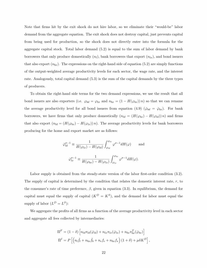
Note that firms hit by the exit shock do not hire labor, so we eliminate their “would-be” labor

demand from the aggregate equation. The exit shock does not destroy capital, just prevents capital

from being used for production, so the shock does not directly enter into the formula for the

aggregate capital stock. Total labor demand (5.2) is equal to the sum of labor demand by bank

borrowers that only produce domestically (nl), bank borrowers that export (nlx), and bond issuers

that also export (nbx). The expressions on the right-hand side of equation (5.2) are simply functions

of the output-weighted average productivity levels for each sector, the wage rate, and the interest

rate. Analogously, total capital demand (5.3) is the sum of the capital demands by the three types

of producers.

To obtain the right-hand side terms for the two demand expressions, we use the result that all

bond issuers are also exporters (i.e. ϕbd = ϕbx and nbx = (1−H(ϕbx))n) so that we can rename

the average productivity level for all bond issuers from equation (4.9) (ϕ̄bd = ϕ̄bx). For bank

borrowers, we have firms that only produce domestically (nld = (H(ϕbx)−H(ϕld))n) and firms

that also export (nld = (H(ϕbx)−H(ϕlx))n). The average productivity levels for bank borrowers

producing for the home and export market are as follows:

ϕ̄σ−1ld ≡ 1

H(ϕlx)−H(ϕld)

∫ ϕlx

ϕld

ϕσ−1dH(ϕ) and

ϕ̄σ−1lx ≡ 1

H(ϕbx)−H(ϕlx)

∫ ϕbx

ϕlx

ϕσ−1dH(ϕ).

Labor supply is obtained from the steady-state version of the labor first-order condition (3.2).

The supply of capital is determined by the condition that relates the domestic interest rate, r, to

the consumer’s rate of time preference, β, given in equation (3.3). In equilibrium, the demand for

capital must equal the supply of capital (KD = KS), and the demand for labor must equal the

supply of labor (LD = LS):

We aggregate the profits of all firms as a function of the average productivity level in each sector

and aggregate all fees collected by intermediaries:

ΠF = (1− δ)[nldπld(ϕ̄ld) + nlxπlx(ϕ̄lx) + nbxπ

Tbx(ϕ̄bx)

]ΠI = P

[(nlf̃l + nbxf̃b + nefe + nbxfx

)(1 + δ) + µδKD

],

22

where the average productivity level for all bank borrowers ϕ̄ld is given by equation (4.8).

As in Melitz (2003), we use a free entry condition to determine the number of firms in steady

state and assume that firm managers are risk-neutral. Let π̄T denote average total profit per firm.

We show in the appendix that ex ante, average profits are given by

π̄T = nldnπld (ϕ̄ld) + nlx

nπlx (ϕ̄lx) + nbx

nπbd (ϕ̄bx) + nbx

nπbx (ϕ̄bx) .

Discounting by the probability of a forced exit shock in each period, δ, yields a simple expression

for the present discounted value of all future profits, which must equal the fixed entry fee, fe, in

equilibrium:

( 11− β(1− δ)

)π̄T ≡Pfe

π̄T = [1− β(1− δ)]Pfe.(5.4)

In steady state, it is straightforward to show that the total value of expenditures (revenues)

PY equals the total number of firms n times average firm revenues ρ (P × Y = nρ). Profits and

revenues are related as follows

πjk(ϕ) = ρjk(ϕ)σ

− P f̃j ,

where ρjk = pj(ϕ)yjk(ϕ), j ∈ {b, l}, and k ∈ {d, x}. Thus, we can obtain an expression for the

number of firms, n as a function of total revenues and the average per-firm revenue:

n = PY

ρ̄

= PY

σ(1− δ)(π̄T

1−δ + nld+nlxn P f̃l + nbx

n P f̃b + nlx+nbxn Pfx

) . (5.5)

Substituting π̄ from equation (5.4) into equation (5.5) yields

n = PY

σ(1− δ){

[1−β(1−δ)]Pfe1−δ + nld+nlx

n P f̃l + nbxn P f̃b + nlx+nbx

n Pfx}

= Y

σ(1− δ){

[1−β(1−δ)]fe1−δ + [H(ϕbx)−H(ϕl)] f̃l + [1−H(ϕbx)] f̃b + [1−H(ϕlx)] fx

} . (5.6)

We put together the equations for the aggregate budget constraint (5.1), aggregate labor de-

23

mand (5.2), aggregate labor supply (3.2), aggregate capital demand (5.3), aggregate capital sup-

ply (3.3), final output technology (4.1), domestic output technology (4.6), domestic and foreign

demand for intermediate goods ( (4.2) and (4.4)), the equation that relates the bank rate to the

bond rate (3.4), the definition of the domestic price level (4.7) and the aggregate price level (4.3),

as well as the conditions that pin down the marginal productivity levels for the marginal pro-

ducer (4.11), the marginal exporter (4.12), the marginal bond issuer (4.13), and the number of

firms (5.6). Using the calibration that we discuss below, we solve for aggregate values (output Y ,

household consumption C) the level of financing (by bank borrowers, Kld+Klx and by bond issuers

Kbd +Kbx), sectoral output (yd and ym), the marginal productivity levels (for domestic producers,

ϕld, exporters, ϕlx, and bond issuers ϕbx), the number of firms n, and the relative prices (the

domestic aggregate price level P , the domestic price level pd, the wage rate w, and the two interest

rates rb and rl). For the numerical analysis we make the standard assumption that idiosyncratic

productivity draws are Pareto distributed, so that H(ϕ) = 1− ϕ−θ.

Conceptually, our model where firms pay a higher fixed cost to attain a lower marginal cost of

financing draws on the mechanics in models of technology upgrading by Yeaple (2005) and Bustos

(2009), where an endogenous number of firms has the option to pay a higher fixed cost to attain a

lower marginal cost. Our model differs in our interpretation of the institutions driving the fixed and

marginal cost differentials, but also in the fact that we fully endogenize the both the supply and

prices of two factor inputs, labor and capital, so that the entire size and structure of the economy

is endogenous. The disutility of labor in the utility function combines with decreasing marginal

returns to labor and capital, as well as the bottom-heavy distribution of firm-specific efficiency

levels, to allow us to do this. The mechanism allows recursive effects between the labor supply and

the capital stock, as changes in the household labor supply affect household income and thus the

amount of the final output they are willing to devote to savings (capital) versus consumption.

5.2 Calibration

We calibrate the model using a value for the elasticity of substitution between domestic varieties of

intermediate goods, σ = 8, coinciding with findings by Feenstra (1994), Broda andWeinstein (2006),

and Eaton and Kortum (2002). The results are robust to higher and lower values, 4 ≤ σ ≤ 11. We

set θ equal to σ so that the output-weighted distribution of efficiency parameters (θ−(σ−1)) equals

24

1, a lower bound for the range found by Del Gatto, Ottaviano, and Pagnini (2008). The elasticity

of substitution between domestic varieties and imported intermediate goods must be lower than σ

for the model to converge in the numeric simulations. We choose ε = 2 as per Ruhl (2004) and

Feenstra, Obstfeld, and Russ (2009). We choose a world export market, Y ∗, that is approximately

five times larger than the domestic market. The results are robust to larger values of Y ∗. We

choose this value because the parameter is not the principal focus of the model and assigning this

magnitude allows us to vary the financial parameters of the model freely without violating the

condition for the existence of bank-borrowing exporters, equation (4.14). Composite estimates of

tariffs and transport costs are difficult to pin down, but Hummels (2007) describes levels of τ equal

to approximately 1.06 for the United States and 1.22 for Latin America. We vary τ from 1.05 to

1.25.

For the calibration of the financial friction parameters we follow Russ and Valderrama (2009)

who discuss estimates of fb, fl, µ, and δ. We vary fb from a level twice as large as fl, which

corresponds to estimates for the United States, to a level about 10 times as large as fl, a value

corresponding roughly to Pakistan. Brazil, for instance, would have an intermediate value of bond

issuance costs, approximately five times as large as fl. The parameters µ and δ are more difficult

to calibrate due to the variety of estimations available and the rather new stylized fact that both

vary over the business cycle and are positively correlated (at least in the United States). The

lowest value of “loss given default” in the finance literature, 0.08, is from Portugal for secured loans

after 48 months of recovery effort, which is quite close to the lowest value recorded for the U.S. on

structured loans, 0.13. We choose 0.10 as our lower bound for µ in the experiments below. As our

upper bound, we choose 0.3, which is roughly equal to the average of 0.318 found for Latin America

between 1970 and 1996. These figures also coincide with the range of monitoring costs cited by

Carlstrom and Fuerst (2001), who use estimates of bankruptcy costs to calibrate this parameter.

Estimates of the default rate δ vary widely, from less than 1 percent in South Korea to 6 percent

in Portugal, to almost 12 percent for small businesses in the United States in 2008. We choose a

middle ground of 5 percent, δ = 0.05.

25

6 Bank and bond market frictions in the small open economy

In this section, we show the results of the numerical analysis of the model. First, we analyze the

impact that policies aimed at financial development have on intra-industry reallocation, export

participation, real exchange rates, aggregate output, and welfare. Then, we study how the gains

from trade liberalization depend on the level of financial development of a country. Finally, we study

how changes in trade openness help determine the level of financial development in a country, even

when the primitive financial parameters of the model (the fixed costs and the relative marginal

costs of bank borrowing and bond issuance) do not change.

We first examine the intra-industry reallocation that underlies financial market development in

a small open economy and its implications for trade and aggregate welfare. Figure 2 shows the level

of firm output as a function of a firm’s idiosyncratic productivity level ϕ and how that level changes

as a result of a drop in the fixed cost of bond issuance. As the cost of bond issuance falls, some

firms switch from bank borrowing to bond issuing. The switchers are the most efficient firms that

use bank financing before the reduction in issuance costs. It is striking here that output increases

among these midsize firms, but falls for the largest and smallest firms, who are not switching their

financing choice. This occurs as switchers begin to exploit their new lower cost of financing capital

expenditures by charging lower prices, drawing domestic market share away from nonswitchers and

expanding exports. Moreover, the figure also shows that while the productivity of the marginal

bond issuer (ϕbx) falls, the productivity levels for the marginal producer (ϕld) and the marginal

exporter (ϕlx) increase. So, while more firms are now bond issuers, those new entrants increase

production. Moreover, the lowest productivity bank borrowers exit and the extensive margin of

trade falls.

Table 1 indicates that aggregate output increases when bond fixed costs fb fall (either when

bank monitoring costs µ are high or low), implying that the increase in production among switchers

more than compensates for the reduction among nonswitchers. The capital stock increases, as well,

meaning the size of total private credit increases. Bond issuance increases more than bank lending.

But the reduction in the extensive margin of trade translates to a drop in the aggregate level of

exports. The negative correlation between the ratio of bond issues to bank credit and aggregate

exports conflicts with the positive correlation seen in Figure 1. Thus, our model suggests that

26

policies promoting bond market development do not fully explain actual bond market development

as observed over the long run. We explain below why growth in trade is a more plausible driver of

observed bond market development.

Now compare the results of a drop in the bond issuance cost fb with the results of a drop

in the bank monitoring cost µ. Figure 3 shows the level of firm output as a function of a firm’s

idiosyncratic productivity level. The drop in bank monitoring costs causes a reduction in the

marginal costs of capital for bank borrowers. This allows all bank-borrowing producers to charge

lower prices, capture a greater market share, and increase profits. As a result, some firms that

previously issued bonds switch to borrowing from banks (ϕbx rises). Moreover, the lower marginal

capital costs apply to all bank borrowers, both previous exporters and nonexporters. Thus, there

is entry into exporting (ϕlx drops) and into production (ϕld drops). As the last column of Table 1

shows, a drop in bank monitoring costs leads to an increase in aggregate output, which increases

labor demand and real wages, increasing marginal costs for all firms. As the figure shows, output

is reallocated toward relatively less efficient firms who charge relatively higher prices both because

of their inferior efficiency and because all bank borrowers still pay higher marginal costs for credit

than bond issuers).

The critical point is that the switchers are also exporters. It is here that the theory of firm

size and bond market development intersects with modern trade theory. When firms switch from

bank loans to bond issues as the issuance cost fb decreases, or reap the benefits of lower interest

rates as monitoring costs (µ) fall, the reduced cost of financing capital expenditures directly results

in lower marginal costs of production. The drop in marginal costs affects both the intensive and

extensive margin of exports. What is more, the two policies each impact the extensive margin and

the aggregate level of exports differently.

Figure 4 depicts the extensive margin of trade (nlx + nbx) as trade costs vary for given levels

of the parameters that determine bond and bank frictions and the trade costs. The top three lines

graph the extensive margin of trade when export entry is “cheap” (fx = fl). The bottom three lines

graph the extensive margin of trade when export entry is “expensive” (fx = 10 × fl). The solid

black lines graph the extensive margin of trade when financial frictions are “high” (fb = 5, µ = 0.3).

The dotted lines show how the extensive margin of trade changes when bond issuance costs fall

(fb = 5). The dashed lines show how the extensive margin of trade changes when bank monitoring

27

costs fall (µ = 0.1).

Figure 4 reveals that increased bank efficiency (a drop in µ) has a big positive impact on

the extensive margin of trade and, as we see in Table 1, increases aggregate exports. Smaller

monitoring costs allow many more firms to export because the high marginal cost of capital financed

through bank borrowing is the principal obstacle for the marginal exporter when fx is low. Smaller

monitoring costs also allow incumbent bank borrowers to slash their prices, increasing market

demand for their exports. Conversely, reducing the fixed cost of bond issuance fb shrinks the

extensive margin and aggregate exports. The switching into bond issuance by medium-sized firms

pulls market share away from the less-efficient smaller firms who must stick with financing through

bank loans with higher interest rates. Competing with the suddenly even lower prices of their

more efficient rivals who switch to bond issues forces the least productive exporters, who remain

dependent on expensive bank credit, to quit exporting. The effects on the extensive margin of trade

are much smaller but work in the same direction if a large fixed cost of exporting dampens firms’

ability to switch into exporting when their marginal costs of financing fall.

The increase in output under both sets of experiments translates into rising consumption, yield-

ing the outcome seen in Figure 5b: lowering bond issuance costs and lowering bank monitoring costs

result in rising welfare. When the banking sector is less efficient (µ is high) switching has a bigger

effect on firms’ marginal costs and their output prices. This means the switching also pushes down

the aggregate price level and boosts the real wage more than when the monitoring costs are low.

Table 1 shows that the real wage increases twice as much in response to a drop in fb when µ is high

compared to when µ is low. As a result, we see in Figure 5b that reducing bond market frictions

gives the biggest boost to welfare when monitoring costs or other similar frictions in the banking

sector are high.

6.1 Financial choice and the gains from trade openness

As discussed above, a number of studies have brought to light the influence that financial frictions

have on gains from trade through comparative advantage. Here, all gains from trade occur through

intra-industry reallocation and financial switching. Not surprisingly, gains from trade can vary to

the degree that export volume increases given various levels of financial transaction costs. Under

our balanced trade condition, greater aggregate export volume allows the small country’s firm

28

managers to purchase more standardized bundles of an imported intermediate good and is correlated

with increases in aggreage output. However, there is a second channel for gains from trade to

emerge through financial switching. Trade liberalization increases the size of the export market,

allowing the biggest bank-dependent exporters to tackle the large issuance cost with the extra

export revenues and begin to issue bonds. Firms switching to bond issuance have lower marginal

costs and therefore cut prices, boosting output, the real wage, and welfare. The financial switching

channel is strongest when issuance costs are low.

Figure 6 depicts the level of the small open economy’s steady-state read GDP (Y ) as a function

of iceberg trade costs τ for given levels of the parameters that determine bond and bank frictions

and fixed trade costs. The solid black line graphs welfare for each level of τ when financial frictions

are “high” (fb = 5, µ = 0.3). The dotted line shows how welfare changes when bond issuance

costs fall (fb = 1). The dashed line shows how welfare changes when bank monitoring costs

fall (µ = 0.1). Aggregate output clearly increases when trade costs fall, regardless of the level

of financial transaction costs. Likewise, aggregate output increases when either type of financial

transaction cost falls, regardless of the degree of trade liberalization. However, the gains from

trade in terms of output growth per incremental drop in τ– reflected in the slopes of the lines–

are slightly larger when the issuance cost falls, as opposed to when monitoring costs fall. This is

not to say that one policy is optimal, only to illustrate that targeted financial policies affect gains

from trade liberalization differently. Because lowering the issuance cost by itself reduces aggregate

exports, it is clear that the increased gains from trade that materialize when issuance costs are low

stem from the financial switching channel, not from trade volume. Gains from trade actually fall

slightly when bank monitoring costs are low because low interest rates on bank loans strengthen

the spillover effect from increased imports, which pulls new firms into active production from the

bottom end of the efficiency spectrum. The amplified reallocation of domestic production toward

the lower end of the efficiency spectrum for each incremental reduction in τ dampens the gains

from trade compared to when monitoring costs are high.

Increasing the fixed trade cost fx (not shown here) lowers output for any given level of iceberg

costs regardless of the level of financial transaction costs. Increasing fx does not alter the order or

slopes seen in Figure 6. Nonetheless, a high fixed cost of exporting dampens the ability of bank

borrowers who serve only the domestic market to switch into exporting. Thus, it reduces the output

29

and welfare gains attained when reducing bank monitoring costs relative to those attained when

reducing bond issuance costs.18

6.2 Intra-industry reallocation and the real exchange rate

Reducing bond issuance costs and lowering bank monitoring costs have opposite effects on the real

exchange rate. The exit of the least productive firms from the domestic market when fb falls, as

described in the previous section, combines with the price reductions by firms switching from banks

to bonds and pushes down the aggregate price level. The real exchange rate depreciates as domestic

goods become cheaper relative to foreign goods.

Figure 7 depicts the log level of the real exchange rate as a function of the bond issuance cost fb

for two different levels of bank monitoring costs, “high” (µ = 0.3) and “low” (µ = 0.1). An increase

in the real exchange rate represents a real exchange rate depreciation. Figure 7 shows that the real

exchange rate depreciates as the bond issuance cost drops. It also demonstrates that regardless

of the level of transaction costs in the bond market, reducing the bank monitoring cost causes a

real exchange rate appreciation. This occurs for two reasons. First, cheaper interest rates on bank

loans allow new, small firms to enter the market. Each additional new firm is less efficient than

the last and absorbs market share from more efficient incumbents because final goods producers

are willing to pay somewhat higher prices to add extra varieties to their assembly process. The

second reason is that, when banks become more efficient, marginal bond issuers switch to bank

loans as their choice for external financing. Since bank loans carry higher marginal costs because

of the assumption of constant CES markups, this means the switchers charge higher prices. The

last three columns in Table 1 demonstrate that the aggregate price level drops when issuance costs

fall, but actually rises a bit when monitoring costs fall, which moves the exchange rate in opposite

directions.18The influence of the size of fx on welfare is not linear beyond the point when it is large enough to push bank

borrowers out of the export market. When it is outlandishly large (fx = 175, 17 times the size of the cost of bondissuance), only a very small fraction of bond issuers (no bank borrowers) are exporters. As in the previous cases,lowering banks’ monitoring costs still increases welfare, but lowering the cost of bond issuance increases the extensivemargin of trade and, by pulling resources away from production for domestic consumption, actually has almost zerowelfare effect.

30

6.3 The impact of trade policy on financial development and the real exchange

rate

Trade policy by itself can influence firms’ choice of financial instrument, influencing aggregate

measures of financial development. Figure 8 depicts the level of a firm’s output as a function of

the idiosyncratic productivity parameter ϕ for two different levels of trade costs, “high” (τ = 1.25)

and “low” (τ = 1.05). In Figure 8, we see that both bond issuance and bank borrowing increase

along the extensive margin and drop on the intensive margin among exporters when trade costs

fall. Falling trade costs allow exporters to expand in number, but with decreased output per firm

as expansion by new exporters pushes up the real wage.

Table 2 shows that the net effect of a reduction of the iceberg trade cost τ on both types of credit

is positive—both bond issuance and bank borrowing increase as an economy becomes more open

to trade. The amount of bank loans increases among nonexporters as the complementarity effect

from export growth boosts demand for domestic varieties and allows more small firms (all bank

borrowers) to start producing. Some domestic bank borrowers also switch to exporting, further

increasing the demand for bank credit. This entry outweighs the drop in the per-firm demand

for bank loans among incumbent bank-borrowing exporters and nonexporters, who reduce their

output a bit due to the new competition for domestic market share and the increasing real wages.

Nonetheless, it is overshadowed by the net increase in bond issues, as the reduction in trade cost

allows the largest exporting bank borrowers to switch to bond issues. The increase in demand

for bond issues relative to bank credit as trade costs fall holds regardless of the level of financial

development in our experiments.

This type of trade liberalization improves common measures of financial market development.

Figure 9 depicts three common measures of financial market development, the stock of credit

as a ratio of GDP and the stock of bond issues as a ratio of the stock of total private credit,

and the stock of bond issues relative to bank credit. All rise as iceberg trade costs fall, simply

because decreasing the iceberg trade cost expands the extensive and intensive margin of trade

and because the resulting boost in imported intermediate goods stimulates additional demand for

domestic intermediate varieties, prompting the entry of new nonexporting suppliers. Increased

export revenues allow the very largest bank borrowers to cover the large bond issuance cost and

31

begin issuing bonds, increasing the total level of bond issues despite the reallocation of production

away from incumbent issuers. The increased demand for domestic varieties to complement the jump

in imports (brought about through the balanced trade condition when exports increase) draws new

domestic producers into the market. Their demand for bank loans, as well as increased demand

for loans by a fraction of bank borrowers who expand into exporting, also boost the level of total

bank credit. Because the firms switching into bond issuance are much larger than the new and

expanding bank borrowers, bond issuance rises relative to bank borrowing, as well as as a share

of total private credit and as a share of GDP: the relative size of the bond market increases along

with exports. Our purpose is to provide a unified analytical framework to address such patterns,

not to test them with formal empirical analyses. However, the positive relationship between the

ratio of bond issues to bank credit and export growth seen in Figure 1 suggests that within the

context of our model, growth in trade is driving growth in the relative size of bond markets over

the long term, rather than reductions in bond market transactions costs.

The last column of Table 2 shows that the type of trade openness a country pursues also has an

effect on its pattern of financial development. Earlier, we noted that a low fixed cost of exporting

allows more switching into exporting by bank borrowers when bank monitoring costs fall. In the

last column of Table 2, we again see this sensitivity of bank borrowers to the size of the fixed export

cost. If trade liberalization focuses on fixed barriers to export participation, rather than ad valorem

tariffs and transport costs, the growth of bank borrowers who suddenly begin exporting (evident in

the rising value of nlx and falling value of ϕlx) increases the aggregate level of bank credit relative

to bond issuance. In fact, the rising real wage makes some bond issuers unable to cover the large

fixed cost of issuance, forcing them to switch to bank borrowing, indicated by the drop in nbx and

the rise in ϕbx. This switching results in a drop in aggregate exports.

When iceberg trade costs fall, the expanded production of the largest bank borrowers switching

into bond issuance is directed in large part toward the export market. The entry of small, less effi-

cient domestic producers therefore can push up the domestic price level and causes a real exchange

rate appreciation. The appreciation is greatest when bank monitoring costs are low, which allows

for more entry by the small new high-cost domestic producers. It is weakest when the fixed cost of

bond issuance costs are small, so that more bank-borrowing exporters switch to the low-yield bond

issues and their decreased marginal costs (and prices) dampen the effect of new entry by small

32

firms on the aggregate domestic price level.

7 Conclusions

In this paper, we have introduced the concept of financial choice into a modern model of trade in a

small open economy. While previous trade literature has examined the impact of singular financial

frictions, we depart from this simplifying assumption and examine the effect of financial choice—the

existence of more than one source of financing for capital investment, where each source carries

different levels of transaction costs. We calibrate transaction costs for bank loans characterized by

higher interest rates and lower fixed costs than for bond issues, in accordance with stylized facts

from studies of financial markets.

Using comparative statics, we find that although both policies increase domestic output, con-

sumption, and welfare, subsidizing bank credit or improving efficiency in the banking sector has

a very different effect on the extensive margin of trade and the real exchange rate in comparison

with policies that increase access to the bond market by reducing the fixed cost of bond issuance.

Policies favoring bank credit cause a reallocation of output and profit toward firms with higher

marginal costs, as they induce some potential bond issuers to switch to using bank loans and allow

new firms to enter at the bottom end of the efficiency continuum. The result is an appreciation of

the real exchange rate but also an increase in the extensive margin of trade and aggregate exports,

as some incumbent bank borrowers find that lower interest rates allow them to start exporting

profitably or to expand their volume of exports.

In contrast, increasing access to the bond market (lowering the fixed cost of issuance) causes

mid- to large-sized firms to switch from bank loans with high interest rates to low-yield bonds.

The reduced cost of capital allows switchers to charge lower prices, boosting their market share

in the domestic and world markets. The result is a real exchange rate depreciation. Reducing

bond issuance costs generates a very small negative impact on the extensive margin of trade as

nonswitchers (incumbent bank borrowers who continue using bank loans) grapple with higher real

wages and reduced domestic market share owing to increased competition from switchers, though

aggregate exports rise because of an increase in the intensive margin. Gains from trade liberalization

are amplified when the fixed costs of bond issuance are low through a financial switching channel:

33

scale effects from widening export markets help more firms begin to issue bonds, lowering their

marginal costs and the aggregate price level.

We also demonstrate that trade liberalization by itself can drive measures of financial devel-

opment. By increasing exports among the mid-size bank borrowers and all (large) bond issuers, a

drop in iceberg trade costs increases the aggregate level of bond issues relative to bank credit, as

well as the overall volume of exports. Though we do not test the model empirically, the positive

correlation between aggregate exports and the ratio of total bond issuance to bank credit is consis-

tent with observed patterns of exports and financial development at long horizons. We also show

that gains from incremental reductions in iceberg trade costs are somewhat larger when the fixed

costs of bond issuance are low due to a financial switching channel, but that low bank monitoring

costs dampen gains from trade liberalization by amplifying a trade spillover effect that pulls less

efficient new firms into active production.

The analysis leaves a number of open questions. We have not considered participation by foreign

banks or financial institutions, which obviously are influential players in the domestic financial mar-

kets of small open economies. Consideration of financial choice in large open economies could reveal

insights into the transmission of business cycles across countries. In particular, bank monitoring

costs and the default rate vary over the business cycle, which may affect capital flows and current

account adjustment in response to various domestic and foreign macroeconomic shocks. Finally and

perhaps most importantly, the banking sector in this model is perfectly competitive, leaving any

interactions between bond market development and the market power of banks unexplored. These

complexities leave interesting paths for future research, but do not detract from our central finding

that firms’ choices between different financial instruments and their export decisions interact with

nontrivial implications for the intensive and extensive margins of trade, the real exchange rate, and

welfare.

34

8 References

Antràs, P., and R. Caballero (2009): “Trade and Capital Flows: A Financial Frictions Per-

spective,” Journal of Political Economy, 117(4), 701–744.

Baliga, S., and B. Polak (2004): “The Emergence and Persistence of the Anglo-Saxon and

German Financial Systems,” The Review of Financial Studies, 17(1), 129–163.

Bardhan, P., and K. Kletzer (1987): “Credit Markets and Patterns of International Trade,”

Journal of Development Economics, 27(1), 57–70.

Broda, C., and D. E. Weinstein (2006): “Globalization and the Gains from Variety,” The

Quarterly Journal of Economics, 121(2), 541–585.

Burger, J. D., and F. E. Warnock (2006): “Local Currency Bond Markets,” IMF Staff papers,

53(Special Issue), 133–146.

Bustos, P. (2009): “Trade Liberalization, Exports and Technology Upgrading: Evidence on the

impact of MERCOSUR on Argentinean Firms,” Forthcoming, American Economic Review.

Carlstrom, C. T., and T. S. Fuerst (1997): “Agency Costs, Net Worth, and Business Fluctu-

ations: A Computable General Equilibrium Analysis,” The American Economic Review, 87(5),

893–910.

(2001): “Monetary shocks, agency costs, and business cycles,” Carnegie-Rochester Con-

ference Series on Public Policy, 54(1), 1 – 27.

Chaney, T. (2005): “Liquidity Constrained Exporters,” Working paper, University of Chicago.

De Fiore, F., and H. Uhlig (2005): “Bank Finance versus Bond Finance: What Explains the

Differences between US and Europe?,” Working Paper 547, European Central Bank.

Del Gatto, M., I. G. Ottaviano, and M. Pagnini (2008): “Openness to Trade and Industry

Cost Dispersion: Evidence from a Panel of Italian Firms,” Journal of Regional Sciences, 48(1),

97–129.

35

Diamond, D. W. (1991): “Monitoring and Reputation: The Choice between Bank Loans and

Directly Placed Debt,” Journal of Political Economy, 99(4), 689–721.

Do, Q.-T., and A. A. Levchenko (2007): “Comparative Advantage, Demand for External

Finance, and Financial Development,” Journal of Development Economics, 86(3), 796–834.

Dunne, T., M. J. Roberts, and L. Samuelson (1988): “Patterns of Firm Entry and Exit in

U.S. Manufacturing Industries,” The RAND Journal of Economics, 19(4), 495–515.

Eaton, J., and S. Kortum (2002): “Technology, Geography, and Trade,” Econometrica, 70(5),

1741–1779.

Endo, T. (2008): “Broadening the offering choice of corporate bonds in emerging markets: Cost-

effective access to debt capital,” Policy Research Working Paper 4655, The World Bank.

Feenstra, R. C. (1994): “New Product Varieties and the Measurement of International Prices,”

The American Economic Review, 84(1), 157–177.

Feenstra, R. C., M. Obstfeld, and K. N. Russ (2009): “In Search of the Armington Elastic-

ity,” Unpublished manuscript, University of California, Davis.

Fillat, J. L., and S. Garreto (2009): “Risk, Returns, and Multinational Production,”

Manuscript, Boston University.

Freixas, X., and J.-C. Rochet (1997): Microeconomics of Banking. MIT Press.

Ghironi, F., and M. J. Melitz (2005): “International Trade and Macroeconomic Dynamics with

Heterogeneous Firms,” The Quarterly Journal of Economics, 120, 381–411.

Greenspan, A. (1999): “Lessons from the Global Crises’,” remarks before the World Bank Group

and the International Monetary Fund, Program of Seminars, Washington, D.C.

Hong Kong Monetary Authority (2001): “Cost-Benefit Analysis of Developing Bond Mar-

kets,” in Quarterly Bulletin, vol. 29.

Hummels, D. (2007): “Transportation Costs and International Trade in the Second Era of Glob-

alization,” Journal of Economic Perspectives, 21(3), 131–154.

36

Levchenko, A. A., R. Rancière, and M. Thoenig (2009): “Growth and Risk at the Industry

Level: The Real Effects of Financial Liberalization,” Journal of Development Economics, 89,

210–222.

Manova, K. (2008): “Credit constraints, equity market liberalizations and international trade,”

Journal of International Economics, 76(1), 33–47.

Melitz, M. J. (2003): “The Impact of Trade on Intra-Industry Reallocations and Aggregate

Industry Productivity,” Econometrica, 71(6), 1695–1725.

Mundell, R. A. (1957): “International Trade and Factor Mobility,” The American Economic

Review, 47, 321–55.

Razin, A., and E. Sadka (2007): Foreign Direct Investment: Analysis of Aggregate Flows. Prince-

ton University Press, Princeton, NJ.

Ruhl, K. J. (2004): “The International Elasticity Puzzle,” Discussion paper, NYU Stern School

of Business.

Russ, K. N. (2009): “The New Theory of Foreign Direct Investment: Merging Trade and Capital

Flows,” International Finance, 12(1), 107–119.

Russ, K. N., and D. Valderrama (2009): “A Theory of Banks, Bonds, and the Distribution of

Firm Size,” Working Paper 15454, National Bureau of Economic Research.

Smith, K. A., and D. Valderrama (2009): “The composition of capital inflows when emerging

market firms face financing constraints,” Journal of Development Economics, 89(2), 223–234.

World Bank, and International Monetary Fund (2001): Developing Government Bond

Markets : A Handbook. World Bank : International Monetary Fund, Washington, D.C.

Yeaple, S. (2005): “A Simple Model of Firm Heterogeneity, Trade, and Wages,” Journal of

International Economics, 65(1), 1–20.

37

A Derivation of bank interest rate and bond yield

We assume that firms must borrow to finance their capital expenditures. In addition, intermedi-

aries also front the fixed financing fees, which are paid with interest after firms collect their sales

revenues.19 An intermediary’s participation constraint implies that the expected cost of monitor-

ing nonperforming loans or defaulted bonds is equal to the expected gains from making loans to

successful firms who repay loans or bond issues with no monitoring (no default),

δnjµjP (K̄ + fj) = (1− δ)nj(rj − r)P (K̄ + fj), j ∈ {l, b}

where P (K̄ + fj) is the average loan size, µj is the monitoring cost, and rj − r is the net return

on earned interest revenues after paying interest on bank deposits or to bond purchasers (the

intermediaries earn the spread as part of the underwriting process). Note that default means (1)

the intermediary incurs monitoring cost µj and receives no interest on loans.

Solving for rj , we obtain the interest rate on loans or bond issues as a function of the risk-free

interest rate from the consumer’s problem:

rj = r + δµj1− δ .

We assume that the monitoring costs for bond investors is less than the monitoring cost for bank

loans, corresponding with the financial literature on monitored versus unmonitored lending. If µl

is greater than µb, then rl > rb. For simplicity and without loss of generality, we assume that µb

equals zero, so that

r = rb = r + δµb1− δ .

B All bond holders export when some bank borrowers export

We assert that if some bank borrowers export, then all bond issuers export and offer a proof by

contradiction:19This assumption simplifies the solution for the interest rate spread, but is not necessary for the results of the

model.

38

Proof. Suppose that at least one bank borrower exports and at least one bond issuer does not

export, so that there exists some ϕb < ϕbx. Given the condition in equation (4.10) holds, then we

have one of two cases—either there exists a set of thresholds ϕl, ϕb, ϕlx, ϕbx such that either:

ϕl < ϕb < ϕlx < ϕbx; (Case I)

ϕl < ϕb < ϕbx < ϕlx, (Case II)

holds.

In Case I, the marginal bond issuer serving only the domestic market must be indifferent between

using bank and bond financing (πbd(ϕb) = πld(ϕb)) and the marginal exporting bond issuer must

also be indifferent between bank and bond financing (πTb (ϕbx) = πTl (ϕbx)).

Substitution in the relevant profit functions, the first condition yields

πbd(ϕb) ≡ πld(ϕb)

pb(ϕb)1−σpσ−εd P εY − Pfb = pl(ϕb)1−σpσ−εd P εY − Pfl

pb(ϕb)1−σ − pl(ϕl)1−σ = P (fb − fl)pσ−εd P εY

ϕσ−1b = P (fb − fl)

pσ−εd P εY

(wα

αα(1− α)(1−α)

)σ−1 (r

(1−σ)(1−α)b − r(1−σ)(1−α)

l

)−1.

(B.1)

Again substituting in the relevant profit functions, the second condition yields

ϕσ−1bx = P (fb − fl)

pσ−εd P εY + τ−σY ∗

(αα(1− α)(1−α)

wα

)σ−1 (r

(1−σ)(1−α)b − r(1−σ)(1−α)

l

)−1. (B.2)

However, because τ−σY ∗ > 0, the right-hand side of equation (B.1) is strictly greater than the

right-hand side of (B.2). This violates the condition that ϕbx must be greater than ϕb if some bond

issuers do not export. Thus, these two conditions cannot both be true.

For Case II to be possible, the marginal exporting bank borrower must be indifferent between

bank and bond finance (πTb (ϕlx) = πTl (ϕlx)) and the marginal exporting bond issuer must prefer

bond to bank financing (πTb (ϕbx) > πTl (ϕbx)).

39

The first condition yields

ϕσ−1lx = P (fb − fl)

pσ−εd P εY

(wα

αα(1− α)(1−α)

)σ−1 (r

(1−σ)(1−α)b − r(1−σ)(1−α)

l

)−1[1 + τ−σY ∗

pσ−εd P εY

]−1

. (B.3)

The second condition yields

ϕσ−1bx >

P (fb − fl)pσ−εd P εY

(wα

αα(1− α)(1−α)

)σ−1 (r

(1−σ)(1−α)b − r(1−σ)(1−α)

l

)−1[1 + τ−σY ∗

pσ−εd P εY

]−1

. (B.4)

Together, equations (B.3) and (B.4) require that ϕbx be greater than ϕlx, so it cannot be true that

ϕl < ϕb < ϕbx < ϕlx.

C Aggregation

We simplify the expression for profits from domestic sales by a bank borrower:

πld(ϕ) = 1σpl(ϕ)yld(ϕ)− P f̃l

= 1σ

(pl(ϕ)P

)1−σPY − P f̃l

= 1σP σY pl(ϕ)1−σ − P f̃l.

Then total profits from domestic sales by all bank borrowers is:

Πld = 1σP σY

1H(ϕbd)−H(ϕbd)

∫ nld

0

∫ ϕbd

ϕld

pl(ϕ)1−σdH(ϕ)di− nldf̃l

= 1σP σY nldpl(ϕ̄ld)1−σ − nldf̃l

= nldπld(ϕ̄ld).

We can similarly derive Πlx, Πbd, and Πbx, so that aggregate profits (before discounting for the

threat of exit shocks and fluctuations in marginal utility, etc.) equals

ΠT = nldπld(ϕ̄ld) + nlxπlx(ϕ̄lx) + nbxπbd(ϕ̄bd) + nbxπbx(ϕ̄bx).

40

Then

π̄T = ΠT

n.

We derive the aggregate supply of labor and capital in the same way as aggregate profit, using the

set of equations in (4.5).

41

Table1:

Polic

yexpe

riments:cheape

rbo

ndiss

uanc

ean

dba

nkmon

itorin

g

(1)

(2)

(3)

(4)

(1)

→(2)

(3)

→(4)

(1)

→(3)

Highf b,

Highµ

Lowf b,

Highµ

Highf b,

Lowµ

Lowf b,

Lowµ

%Cha

nge

(↓f b

|Highµ)

%Cha

nge

(↓f b

|Low

µ)

%Cha

nge

(↓µ

|Highf b)

µ0.300

0.300

0.100

0.100

0.000

0.000

-66.667

δ0.050

0.050

0.050

0.050

0.000

0.000

0.000

f l0.500

0.500

0.500

0.500

0.000

0.000

-0.900

f b5.000

1.000

5.000

1.000

-80.000

-80.000

0.000

f x0.500

0.500

0.500

0.500

0.000

0.000

0.000

τ1.250

1.250

1.250

1.250

0.000

0.000

0.000

ϕl

1.324

1.338

1.297

1.306

1.116

0.696

-2.020

ϕlx

1.360

1.371

1.339

1.342

0.776

0.272

-1.579

ϕbx

1.908

1.404

2.210

1.621

-26.405

-26.661

15.861

nl

0.121

0.038

0.152

0.122

-68.257

-19.708

25.703

nlx

0.096

0.017

0.118

0.093

-81.895

-21.039

22.457

nbx

0.007

0.083

0.002

0.026

1101.532

1115.755

-68.443

r b0.154

0.154

0.154

0.154

0.000

0.000

0.000

r l0.169

0.169

0.159

0.159

0.000

0.000

-6.218

P0.523

0.521

0.523

0.522

-0.404

-0.314

0.030

Y11.413

11.824

11.677

11.869

3.607

1.644

2.313

C9.986

10.326

10.204

10.367

3.397

1.592

2.181

K14.265

14.989

14.726

15.020

5.077

1.999

3.233

L=w/P

2.747

2.794

2.777

2.799

1.698

0.805

1.084

πF

0.787

0.811

0.807

0.819

2.985

1.440

2.518

K/L

5.192

5.365

5.303

5.366

3.322

1.185

2.126

Exp

orts

7.183

5.947

7.714

6.553

-17.205

-15.048

7.396

Ban

kLo

ans

3.092

0.314

5.228

2.282

-89.839

-56.343

69.087

Bon

dIssues

11.173

14.675

9.498

12.738

31.343

34.113

-14.990

Welfare

6.213

6.423

6.348

6.448

3.380

1.577

2.181

42

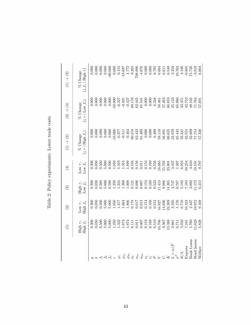
Table2:

Polic

yexpe

riments:Lo

wer

trad

ecosts

(1)

(2)

(3)

(4)

(1)

→(2)

(3)

→(4)

(1)

→(3)

Highτ,

Highf x

Lowτ,

Highf x

Highτ,

Lowf x

Lowτ,

Lowf x

%Cha

nge

(↓τ

|Highf x)

%Cha

nge

(↓τ

|Low

f x)

%Cha

nge

(↓f x

|Highτ)

µ0.300

0.300

0.300

0.300

0.000

0.000

0.000

δ0.050

0.050

0.050

0.050

0.000

0.000

0.000

f l0.500

0.500

0.500

0.500

0.000

0.000

0.000

f b5.000

5.000

5.000

5.000

0.000

0.000

0.000

f x5.000

5.000

0.500

0.500

0.000

0.000

-90.000

τ1.250

1.050

1.250

1.050

-16.000

-16.000

0.000

ϕl

1.322

1.317

1.324

1.319

-0.377

-0.327

0.155

ϕlx

1.673

1.664

1.360

1.354

-0.511

-0.491

-18.697

ϕbx

1.874

1.866

1.908

1.899

-0.464

-0.427

1.772

nl

0.111

0.178

0.121

0.194

60.216

60.176

9.205

nlx

0.011

0.017

0.096

0.156

62.432

62.445

798.006

nbx

0.007

0.012

0.007

0.011

61.409

61.541

-4.676

r b0.154

0.154

0.154

0.154

0.000

0.000

0.000

r l0.169

0.169

0.169

0.169

0.000

0.000

0.000

P0.519

0.552

0.523

0.556

6.409

6.328

0.795

Y10.706

16.927

11.413

18.085

58.110

58.461

6.604

C9.367

14.696

9.986

15.705

56.891

57.263

6.611

K13.388

22.309

14.265

23.801

66.635

66.853

6.548

L=w/P

2.661

3.325

2.747

3.437

24.970

25.123

3.258

πF

0.711

1.176

0.787

1.307

65.443

65.960

10.762

K/L

5.032

6.710

5.192

6.924

33.341

33.351

3.186

Exp

orts

7.241

10.323

7.183

10.254

42.551

42.752

-0.805

Ban

kLo

ans

1.760

2.337

3.092

4.610

32.809

49.105

75.720

Bon

dIssues

11.629

19.972

11.173

19.191

71.754

71.764

-3.919

Welfare

5.828

9.169

6.213

9.797

57.326

57.691

6.604

43

Figure 1: Export growth is associated with an increase in the level of domestic corporate bondissues relative to bank credit

44

Figure 2: Reallocation of output across firm efficiency levels as bond fixed costs fall

45

Figure 3: Reallocation of output across firm efficiency levels as bank monitoring costs fall

46

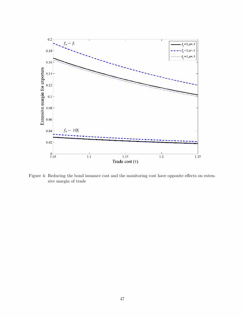
Figure 4: Reducing the bond issuance cost and the monitoring cost have opposite effects on exten-sive margin of trade

47

(a) Issuance costs, monitoring costs, and output

(b) Issuance costs, monitoring costs, and welfare

Figure 5: Aggregate outcomes from altering financial choice

48

Figure 6: Aggregate output increases when trade costs fall

49

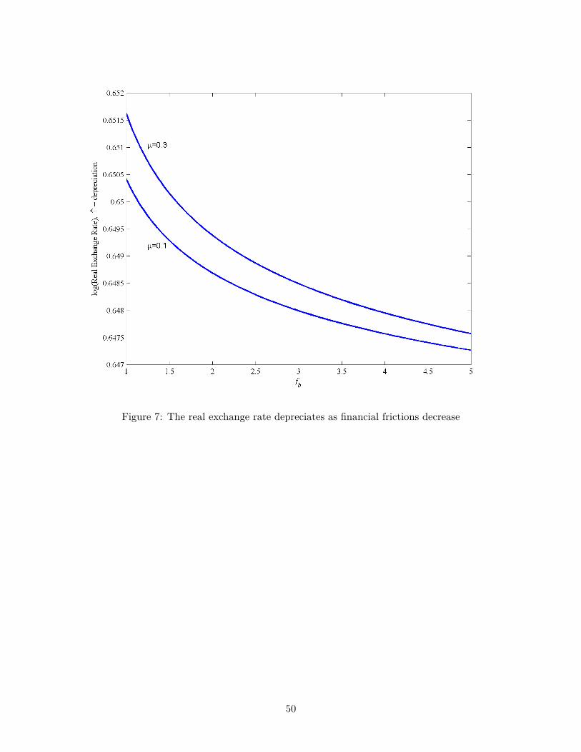
Figure 7: The real exchange rate depreciates as financial frictions decrease

50

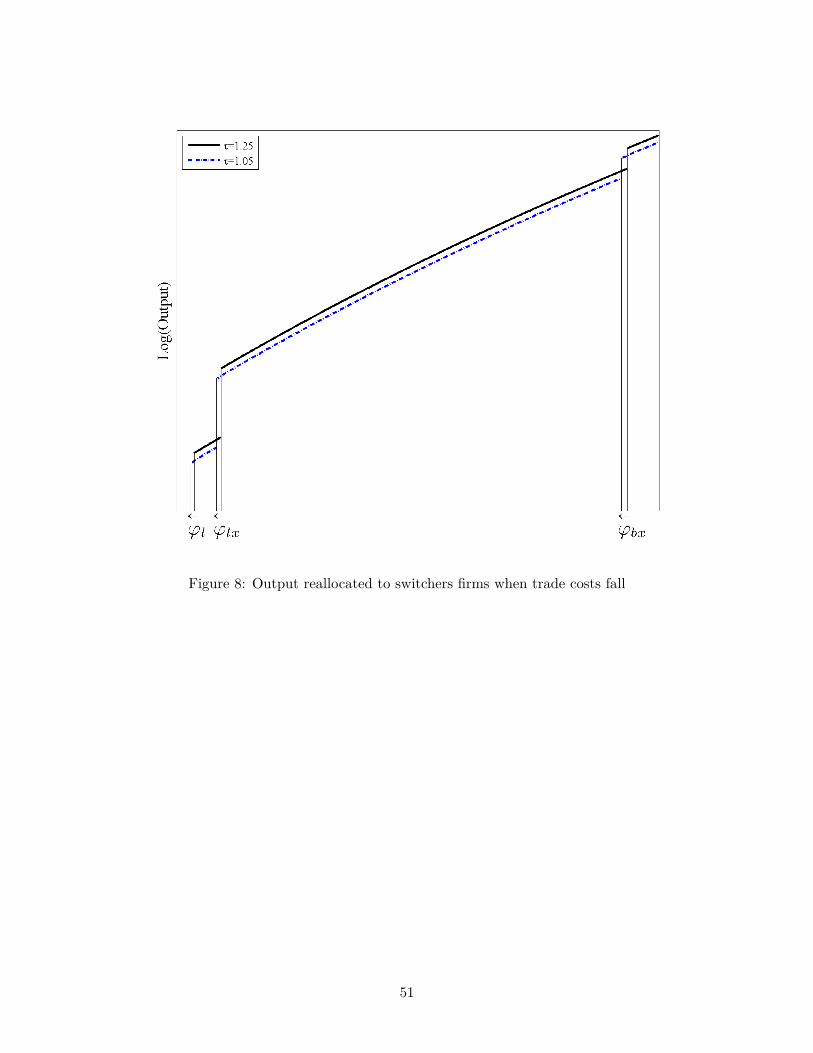
Figure 8: Output reallocated to switchers firms when trade costs fall

51

Figure 9: Trade liberalization causes growth in the relative size of the bond market

52

Figure 10: Trade liberalization causes real exchange rate appreciation

53