Finance Valuation - Valuing Companies by Discounted Cash Flows - Ten Methods and Nine Theories - P...
29
Working Paper Published by PricewaterhouseCoopers Chair of Finance * Professor of Financial Management, IESE IESE Business School - Universidad de Navarra Avda. Pearson, 21 - 08034 Barcelona. Tel.: (+34) 93 253 42 00 Fax: (+34) 93 253 43 43 Camino del Cerro del Águila, 3 (Ctra. de Castilla, km. 5,180) - 28023 Madrid. Tel.: (+34) 91 357 08 09 Fax: (+34) 91 357 29 13 Copyright© 2002, IESE Business School. Do not quote or reproduce without permission WP No 451 January, 2002 VALUING COMPANIES BY DISCOUNTED CASH FLOWS: TEN METHODS AND NINE THEORIES Pablo Fernández * Revised in March, 2004
Transcript of Finance Valuation - Valuing Companies by Discounted Cash Flows - Ten Methods and Nine Theories - P...

Working Paper
PPuubblliisshheedd bbyy PPrriicceewwaatteerrhhoouusseeCCooooppeerrss CChhaaiirr ooff FFiinnaannccee
* Professor of Financial Management, IESE
IESE Business School - Universidad de NavarraAvda. Pearson, 21 - 08034 Barcelona. Tel.: (+34) 93 253 42 00 Fax: (+34) 93 253 43 43Camino del Cerro del Águila, 3 (Ctra. de Castilla, km. 5,180) - 28023 Madrid. Tel.: (+34) 91 357 08 09 Fax: (+34) 91 357 29 13
Copyright© 2002, IESE Business School. Do not quote or reproduce without permission
WP No 451
January, 2002
VALUING COMPANIES BY DISCOUNTED CASH FLOWS:TEN METHODS AND NINE THEORIES
Pablo Fernández *
Revised in March, 2004
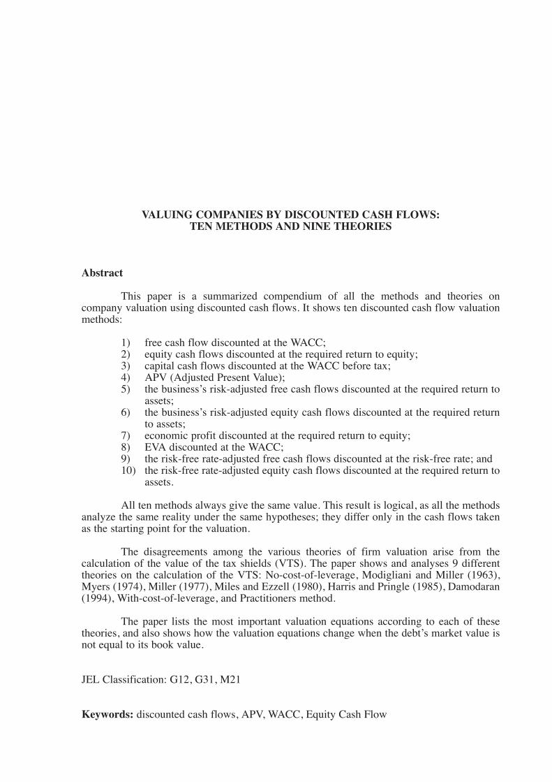
VALUING COMPANIES BY DISCOUNTED CASH FLOWS:TEN METHODS AND NINE THEORIES
Abstract
This paper is a summarized compendium of all the methods and theories oncompany valuation using discounted cash flows. It shows ten discounted cash flow valuationmethods:
1) free cash flow discounted at the WACC; 2) equity cash flows discounted at the required return to equity; 3) capital cash flows discounted at the WACC before tax; 4) APV (Adjusted Present Value); 5) the business’s risk-adjusted free cash flows discounted at the required return to
assets;6) the business’s risk-adjusted equity cash flows discounted at the required return
to assets;7) economic profit discounted at the required return to equity; 8) EVA discounted at the WACC;9) the risk-free rate-adjusted free cash flows discounted at the risk-free rate; and10) the risk-free rate-adjusted equity cash flows discounted at the required return to
assets.
All ten methods always give the same value. This result is logical, as all the methodsanalyze the same reality under the same hypotheses; they differ only in the cash flows takenas the starting point for the valuation.
The disagreements among the various theories of firm valuation arise from thecalculation of the value of the tax shields (VTS). The paper shows and analyses 9 differenttheories on the calculation of the VTS: No-cost-of-leverage, Modigliani and Miller (1963),Myers (1974), Miller (1977), Miles and Ezzell (1980), Harris and Pringle (1985), Damodaran(1994), With-cost-of-leverage, and Practitioners method.
The paper lists the most important valuation equations according to each of thesetheories, and also shows how the valuation equations change when the debt’s market value isnot equal to its book value.
JEL Classification: G12, G31, M21
Keywords: discounted cash flows, APV, WACC, Equity Cash Flow

VALUING COMPANIES BY DISCOUNTED CASH FLOWS:TEN METHODS AND NINE THEORIES
This paper is a summarized compendium of all the methods and theories oncompany valuation using discounted cash flows.
Section 1 shows the ten most commonly used methods for valuing companies bydiscounted cash flows:
1) free cash flow discounted at the WACC; 2) equity cash flows discounted at the required return to equity; 3) capital cash flows discounted at the WACC before tax; 4) APV (Adjusted Present Value); 5) the business’s risk-adjusted free cash flows discounted at the required return to
assets;6) the business’s risk-adjusted equity cash flows discounted at the required return
to assets;7) economic profit discounted at the required return to equity; 8) EVA discounted at the WACC;9) the risk-free rate-adjusted free cash flows discounted at the risk-free rate; and10) the risk-free rate-adjusted equity cash flows discounted at the required return to
assets.
All ten methods always give the same value. This result is logical, since all themethods analyze the same reality under the same hypotheses; they differ only in the cashflows taken as the starting point for the valuation.
In section 2 the ten methods and nine theories are applied to an example. The ninetheories are:
1) No-cost-of-leverage. Assuming that there are no leverage costs.
2) Damodaran (1994). To introduce leverage costs, Damodaran assumes that therelationship between the levered and unlevered beta is1: βL = βu + D (1-T) βu /E
3) Practitioners method. To introduce higher leverage costs, this method assumesthat the relationship between the levered and unlevered beta is: βL = βu + D βu / E
1 Instead of the relationship obtained from No-cost-of-leverage: βL = βu + D (1-T) (βu - βd) / E

4) Harris and Pringle (1985) and Ruback (1995). All of their equations arise fromthe assumption that the leverage-driven value creation or value of tax shields(VTS) is the present value of the tax shields2 discounted at the required returnto the unlevered equity (Ku). According to them,
VTS = PV[D Kd T ; Ku]
5) Myers (1974), who assumes that the value of tax shields (VTS) is the presentvalue of the tax shields discounted at the required return to debt (Kd).According to Myers,
VTS = PV[D Kd T ; Kd]
6) Miles and Ezzell (1980). They state that the correct rate for discounting the taxshield (D Kd T) is Kd for the first year, and Ku for the following years.
7) Miller (1977) concludes that the leverage-driven value creation or value of thetax shields is zero.
8) With-cost-of-leverage. This theory assumes that the cost of leverage is thepresent value of the interest differential that the company pays over the risk-free rate.
9) Modigliani and Miller (1963) calculate the value of tax shields by discountingthe present value of the tax savings due to interest payments of a risk-free debt(T D RF) at the risk-free rate (R F). Modigliani and Miller claim that
VTS = PV[RF; DT RF]
Appendix 1 gives a brief overview of the most significant theories on discountedcash flow valuation.
Appendix 2 contains the valuation equations according to these theories.
Appendix 3 shows how the valuation equations change if the debt’s market value isnot equal to its nominal value.
Appendix 4 contains a list of the abbreviations used in the paper.
1. Ten discounted cash flow methods for valuing companies
There are four basic methods for valuing companies by discounted cash flows:
2
2 The tax shield of a given year is D Kd T. D is the value of debt, Kd is the required return to debt, and T is thecorporate tax rate. D Kd is the interest paid in a given year. The formulas used in the paper are valid ifthe interest rate on the debt matches the required return to debt (Kd), or to put it another way, if the debt’smarket value is identical to its book value. The formulas for when this is not the case are given inAppendix 3.

Method 1. Using the free cash flow and the WACC (weighted average cost ofcapital).
Equation [1] indicates that the value of the debt (D) plus that of the shareholders’equity (E) is the present value of the expected free cash flows (FCF) that the company willgenerate, discounted at the weighted average cost of debt and shareholders’ equity after tax(WACC):
[1] E0 + D0 = PV0 [ WACCt ; FCFt]
The definition of WACC or “weighted average cost of capital” is given by [2]:
[2] WACCt = [ Et-1 Ket + Dt-1 Kdt (1-T)] / [ Et-1 + Dt-1 ]
Ke is the required return to equity, Kd is the cost of the debt, and T is the effectivetax rate applied to earnings. Et-1 + Dt-1 are market values3.
Method 2. Using the expected equity cash flow (ECF) and the required return toequity (Ke).
Equation [3] indicates that the value of the equity (E) is the present value of theexpected equity cash flows (ECF) discounted at the required return to equity (Ke).
[3] E0 = PV0 [ Ket; ECFt]
Equation [4] indicates that the value of the debt (D) is the present value of theexpected debt cash flows (CFd) discounted at the required return to debt (Kd).
[4] D0 = PV0 [ Kdt; CFdt]
The expression that relates the FCF with the ECF is4:
[5] ECFt = FCFt + ∆ Dt - It (1 - T)
∆ Dt is the increase in debt, and It is the interest paid by the company. It is obviousthat CFd = It - ∆ Dt
The sum of the values given by equations [3] and [4] is identical to the valueprovided by [1]5:
E0 + D0 = PV0 [ WACCt; FCFt] = PV0 [ Ket; ECFt] + PV0 [ Kdt; CFdt]
3
3 In actual fact, “market values” are the values obtained when the valuation is performed using formula [1].Consequently, the valuation is an iterative process: the free cash flows are discounted at the WACC tocalculate the company’s value (D+E) but, in order to obtain the WACC, we need to know the company’svalue (D+E).
4 Obviously, the free cash flow is the hypothetical equity cash flow when the company has no debt.5 Indeed, one way of defining the WACC is: the WACC is the rate at which the FCF must be discounted so
that equation [2] gives the same result as that given by the sum of [3] and [4].

Method 3. Using the capital cash flow (CCF) and the WACCBT (weighted averagecost of capital, before tax).
The capital cash flows6 are the cash flows available for all holders of the company’ssecurities, whether these be debt or shares, and are equivalent to the equity cash flow (ECF)plus the cash flow corresponding to the debt holders (CFd).
Equation [6] indicates that the value of the debt today (D) plus that of theshareholders’ equity (E) is equal to the capital cash flow (CCF) discounted at the weightedaverage cost of debt and shareholders’ equity before tax (WACCBT).
[6] E0 + D0 = PV[WACCBT t; CCFt]
The definition of WACCBT is [7]:
[7] WACCBT t = [ Et-1 Ket + Dt-1 Kdt] / [ Et-1 + Dt-1 ]
Expression [7] is obtained by making [1] equal to [6]. WACCBT represents thediscount rate that ensures that the value of the company obtained using the two expressions isthe same7:
E0 + D0 = PV[WACCBT t ; CCFt] = PV[WACCt; FCFt ]
The expression that relates the CCF with the ECF and the FCF is [8]:
[8] CCFt = ECFt + CFdt = ECFt - ∆ Dt + It = FCFt + It T
∆ Dt = Dt - Dt-1; It = Dt-1 Kdt
Method 4. Adjusted present value (APV)
The adjusted present value (APV) equation [9] indicates that the value of the debt(D) plus that of the shareholders’ equity (E) is equal to the value of the unlevered company’sshareholders’ equity, Vu, plus the present value of the value of the tax shield (VTS):
[9] E0 + D0 = Vu0 + DVTS0
We can see in Appendixes 1 and 2 that there are several theories for calculating theVTS.
If Ku is the required return to equity in the debt-free company (also called therequired return to assets), Vu is given by [10]:
[10] Vu0 = PV0 [ Kut; FCFt]
4
6 Arditti and Levy (1977) suggested that the firm’s value could be calculated by discounting the capital cashflows instead of the free cash flow.
7 One way of defining the WACCBT is: the WACCBT is the rate at which the CCF must be discounted so thatequation [6] gives the same result as that given by the sum of [3] and [4].

Consequently,
VTS0 = E0 + D0 - Vu0 = PV0 [ WACCt; FCFt] - PV0 [ Kut; FCFt]
We can talk of a fifth method (using the business risk-adjusted free cash flow),although this is not actually a new method but is derived from the previous methods:
Method 5. Using the business risk-adjusted free cash flow and Ku (required returnto assets).
Equation [11] indicates that the value of the debt (D) plus that of the shareholders’equity (E) is the present value of the expected business risk-adjusted free cash flows(FCF\\Ku) that will be generated by the company, discounted at the required return to assets(Ku):
[11] E0 + D0 = PV0 [ Kut ; FCFt\\Ku]
The definition of the business risk-adjusted free cash flows8 (FCF\\Ku) is [12]:
[12] FCFt\\Ku = FCFt - (Et-1 + Dt-1 ) [ WACCt - Kut ]
Likewise, we can talk of a sixth method (using the business risk-adjusted equity cashflow), although this is not actually a new method but is derived from the previous methods:
Method 6. Using the business risk-adjusted equity cash flow and Ku (requiredreturn to assets).
Equation [13] indicates that the value of the equity (E) is the present value of theexpected business risk-adjusted equity cash flows (ECF\\Ku) discounted at the requiredreturn to assets (Ku):
[13] E0 = PV0 [ Kut; ECFt \\Ku]
The definition of the business risk-adjusted equity cash flows9 (ECF\\Ku) is [14]:
[14] ECFt\\Ku = ECFt - Et-1 [ Ket - Kut ]
Method 7. Using the economic profit and Ke (required return to equity).
Equation [15] indicates that the value of the equity (E) is the equity’s book valueplus the present value of the expected economic profit (EP) discounted at the required returnto equity (Ke).
[15] E0 = Evc0 + PV0 [ Ket; EPt]
5
8 Expression [12] is obtained by making [11] equal to [1].9 Expression [14] is obtained by making [13] equal to [3].

The term economic profit (EP) is used to define the accounting net income or profitafter tax (PAT) less the equity’s book value (Ebvt-1) multiplied by the required return toequity.
[16] EPt = PATt - Ke Ebvt-1
Method 8. Using the EVA (economic value added) and the WACC (weightedaverage cost of capital).
Equation [17] indicates that the value of the debt (D) plus that of the shareholders’equity (E) is the book value of the shareholders’ equity and the debt (Ebv0+ N0) plus thepresent value of the expected EVA, discounted at the weighted average cost of capital(WACC):
[17] E0 + D0 = (Ebv0+ N0) + PV0 [ WACCt ; EVAt]
The EVA (economic value added) is the NOPAT (Net Operating Profit After Tax)less the company’s book value (Dt-1 + Ebvt-1) multiplied by the weighted average cost ofcapital (WACC). The NOPAT (Net Operating Profit After Taxes) is the profit of theunlevered company (debt-free).
[18] EVAt = NOPATt - (Dt-1 + Ebvt-1)WACC t
Method 9. Using the risk-free-adjusted free cash flows discounted at the risk-freerate
Equation [19] indicates that the value of the debt (D) plus that of the shareholders’equity (E) is the present value of the expected risk-free-adjusted free cash flows (FCF\\ RF)that will be generated by the company, discounted at the risk-free rate (RF):
[19] E0 + D0 = PV0 [ RF t ; FCFt\\RF]
The definition of the risk-free-adjusted free cash flows10 (FCF\\RF) is [20]:
[20] FCFt\\RF = FCFt - (Et-1 + Dt-1 ) [ WACCt - RF t ]
Likewise, we can talk of a tenth method (using the risk-free-adjusted equity cashflow), although this is not actually a new method but is derived from the previous methods:
Method 10. Using the risk-free-adjusted equity cash flows discounted at the risk-free rate
Equation [21] indicates that the value of the equity (E) is the present value of theexpected risk-free-adjusted equity cash flows (ECF\\RF) discounted at the risk-free rate (RF):
[21] E0 = PV0 [ RF t; ECFt \\RF]
6
10 Expression [20] is obtained by making [19] equal to [1].

The definition of the risk-free-adjusted equity cash flows11 (ECF\\RF) is [22]:
[22] ECFt\\RF = ECFt - Et-1 [ Ket - RF t ]
We could also talk of an eleventh method; using the business risk-adjusted capitalcash flow and Ku (required return to assets), but the business risk-adjusted capital cash flowis identical to the business risk-adjusted free cash flow (CCF\\Ku = FCF\\Ku). Therefore, thismethod would be identical to Method 5.
We could also talk of a twelfth method; using the risk-free-adjusted capital cash flowand RF (risk-free rate), but the risk-free-adjusted capital cash flow is identical to the risk-free-adjusted free cash flow (CCF\\RF = FCF\\RF). Therefore, this method would be identical toMethod 9.
2. An example. Valuation of the company Toro Inc.
The company Toro Inc. has the balance sheet and income statement forecastsfor the next few years shown in Table 1. After year 3, the balance sheet and the incomestatement are expected to grow at an annual rate of 2%.
Table 1. Balance sheet and income statement forecasts for Toro Inc.
0 1 2 3 4 5
WCR (working capital requirements) 400 430 515 550 561.00 572.22Gross fixed assets 1,600 1,800 2,300 2,600 2,913.00 3,232.26- accumulated depreciation 200 450 720 995.40 1,276.31
Net fixed assets 1,600 1,600 1,850 1,880 1,917.60 1,955.95TOTAL ASSETS 2,000 2,030 2,365 2,430 2,478.60 2,528
Debt (N) 1,500 1,500 1,500 1,500 1,530.00 1,560.60Equity (book value) 500 530 865 930 948.60 967.57TOTAL LIABILITIES 2,000 2,030 2,365 2,430 2,478.60 2,528
Income statement
Margin 420 680 740 765.00 780Interest payments 120 120 120 120.00 122PBT (profit before tax) 300 560 620 645.00 658Taxes 105 196 217 225.75 230.27PAT (profit after tax = net income) 195 364 403 419.25 427.64
Using the balance sheet and income statement forecasts in Table 1, we can readilyobtain the cash flows given in Table 2. Obviously, the cash flows grow at a rate of 2% afteryear 4.
7
11 Expression [22] is obtained by making [21] equal to [3].

Table 2. Cash flow forecasts for Toro Inc
1 2 3 4 5
PAT (profit after tax) 195 364 403 419.25 427.64
+ depreciation 200 250.00 270.00 275.40 280.91+ increase of debt 0 0.00 0.00 30.00 30.60- increase of working capital requirements -30 -85 -35 -11 -11.22- investment in fixed assets -200 -500.00 -300.00 -313.00 -319.26
ECF 165.00 29.00 338.00 400.65 408.66
FCF 243.00 107.00 416.00 448.65 457.62
CFd 120.00 120.00 120.00 90.00 91.80
CCF 285.00 149.00 458.00 490.65 500.46
The unlevered beta (βu) is 1. The risk-free rate is 6%. The cost of debt is 8%. Thecorporate tax rate is 35%. The market risk premium is 4%. Consequently, using the CAPM,the required return to assets is 10%.12 With these parameters, the valuation of this company’sequity, using the above equations, is given in Table 3. The required return to equity (Ke)appears in the second line of the table13. Equation [3] enables the value of the equity to beobtained by discounting the equity cash flows at the required return to equity (Ke)14.Likewise, equation [4] enables the value of the debt to be obtained by discounting the debtcash flows at the required return to debt (Kd)15. Another way to calculate the value of theequity is using equation [1]. The present value of the free cash flows discounted at theWACC (equation [2]) gives us the value of the company, which is the value of the debt plusthat of the equity16. By subtracting the value of the debt from this quantity, we obtain thevalue of the equity. Another way of calculating the value of the equity is using equation [6].The present value of the capital cash flows discounted at the WACCBT (equation [7]) gives usthe value of the company, which is the value of the debt plus that of the equity. Bysubtracting the value of the debt from this quantity, we obtain the value of the equity. Thefourth method for calculating the value of the equity is using the Adjusted Present Value,equation [9]. The value of the company is the sum of the value of the unlevered company(equation [10]) plus the present value of the value of the tax shield (VTS)17.
The business risk-adjusted equity cash flow and free cash flow (ECF\\Ku andFCF\\Ku) are also calculated using equations [14] and [12]. Equation [13] enables us toobtain the value of the equity by discounting the business risk-adjusted equity cash flows atthe required return to assets (Ku). Another way to calculate the value of the equity is usingequation [11]. The present value of the business risk-adjusted free cash flows discounted atthe required return to assets (Ku) gives us the value of the company, which is the value of thedebt plus that of the equity. By subtracting the value of the debt from this quantity, we obtainthe value of the equity.
8
12 In this example, we use the CAPM: Ku = RF + βu PM = 6% + 4% = 10%.13 The required return to equity (Ke) has been calculated according to the no-cost-of-leverage theory (see
Appendix 1).14 The relationship between the value of the equity in two consecutive years is: Et = Et-1 (1+Ket) - ECFt15 The value of the debt is equal to the nominal value (book value) given in Table 1 because we have
considered that the required return to debt is equal to its cost (8%).16 The relationship between the company’s value in two consecutive years is:
(D+E)t = (D+E)t-1 (1+WACCt) - FCFt17 As the required return to equity (Ke) has been calculated according to the no-cost-of-leverage theory, we
must also calculate the VTS according to the no-cost-of-leverage theory, namely: VTS = PV (Ku; D T Ku)

The economic profit (EP) is calculated using equation [16]. Equation [15] indicatesthat the value of the equity (E) is the equity’s book value plus the present value of theexpected economic profit (EP) discounted at the required return to equity (Ke).
The EVA (economic value added) is calculated using equation [18]. Equation [17]indicates that the equity value (E) is the present value of the expected EVA discounted at theweighted average cost of capital (WACC), plus the book value of the equity and the debt(Ebv0+ N0) minus the value of the debt (D).
Table 3. Valuation of Toro Inc. No cost of leverage
0 1 2 3 4 5
Ku 10.00% 10.00% 10.00% 10.00% 10.00% 10.00%equation Ke 10.49% 10.46% 10.42% 10.41% 10.41% 10.41%
[1] E+D = PV(WACC;FCF) 5,458.96 5,709.36 6,120.80 6,264.38 6,389.66 6,517.46[2] WACC 9.04% 9.08% 9.14% 9.16% 9.16% 9.16%
[1] - D = E 3,958.96 4,209.36 4,620.80 4,764.38 4,859.66 4,956.86
[3] E = PV(Ke;ECF) 3,958.96 4,209.36 4,620.80 4,764.38 4,859.66 4,956.86
[4] D = PV(CFd;Kd) 1,500.00 1,500.00 1,500.00 1,500.00 1,530.00 1,560.60
[6] D+E = PV(WACCBT;CCF) 5,458.96 5,709.36 6,120.80 6,264.38 6,389.66 6,517.46[7] WACCBT 9.81% 9.82% 9.83% 9.83% 9.83% 9.83%
[6] - D = E 3,958.96 4,209.36 4,620.80 4,764.38 4,859.66 4,956.86
VTS = PV(Ku;D T Ku) 623.61 633.47 644.32 656.25 669.38 682.76[10] Vu = PV(Ku;FCF) 4,835.35 5,075.89 5,476.48 5,608.12 5,720.29 5,834.69[9] VTS + Vu 5,458.96 5,709.36 6,120.80 6,264.37 6,389.66 6,517.46
[9] - D = E 3,958.96 4,209.36 4,620.80 4,764.37 4,859.66 4,956.86
[11] D+E=PV(Ku;FCF\\Ku) 5,458.96 5,709.36 6,120.80 6,264.37 6,389.66 6,517.46[12] FCF\\Ku 295.50 159.50 468.50 501.15 511.17
[11] - D = E 3,958.96 4,209.36 4,620.80 4,764.38 4,859.66 4,956.86
[13] E = PV(Ku;ECF\\Ku) 3,958.96 4,209.36 4,620.80 4,764.38 4,859.66 4,956.86[14] ECF\\Ku 145.50 9.50 318.50 381.15 388.77
[16] EP 142.54 308.54 312.85 322.44 328.89PV(Ke;EP) 3,458.96 3,679.36 3,755.80 3,834.38 3,911.06 3,989.28
[15] PV(Ke;EP) + Ebv = E 3,958.96 4,209.36 4,620.80 4,764.38 4,859.66 4,956.86
[18] EVA 92.23 257.67 264.79 274.62 280.11PV(WACC;EVA) 3,458.96 3,679.36 3,755.80 3,834.38 3,911.06 3,989.28
[17] E=PV(WACC;EVA)+Ebv+N-D 3,958.96 4,209.36 4,620.80 4,764.38 4,859.66 4,956.86
[19] D+E=PV(RF;FCF\\RF) 5,458.96 5,709.36 6,120.80 6,264.38 6,389.66 6,517.46[20] FCF\\RF 77.14 -68.87 223.67 250.58 255.59
[19] - D = E 3,958.96 4,209.36 4,620.80 4,764.38 4,859.66 4,956.86
[21] E=PV(RF;ECF\\RF) 3,958.96 4,209.36 4,620.80 4,764.38 4,859.66 4,956.86[22] ECF\\RF -12.86 -158.87 133.67 190.58 194.39
The risk-free-adjusted equity cash flow and free cash flow (ECF\\RF and FCF\\RF)are also calculated using equations [22] and [20]. Equation [21] enables us to obtain the valueof the equity by discounting the risk-free-adjusted equity cash flows at the risk-free rate (RF).Another way to calculate the value of the equity is using equation [19]. The present value ofthe risk-free-adjusted free cash flows discounted at the required return to assets (RF) gives usthe value of the company, which is the value of the debt plus that of the equity. Bysubtracting the value of the debt from this quantity, we obtain the value of the equity.
9

Table 3 shows that the result obtained with all ten valuations is the same. The valueof the equity today is 3,958.96. As we have already mentioned, these valuations have beenperformed according to the No-cost-of-leverage theory. The valuations performed using othertheories are discussed further on.
Tables 4 to 11 contain the most salient results of the valuation performed on thecompany Toro Inc. according to Damodaran (1994), Practitioners method, Harris and Pringle(1985), Myers (1974), Miles and Ezzell (1980), Miller (1977), With-cost-of-leverage theory,and Modigliani and Miller (1963).
Table 4. Valuation of Toro Inc. according to Damodaran (1994)
0 1 2 3 4 5
VTS = PV[Ku; DTKu - D (Kd- RF) (1-T)] 391.98 398.18 405.00 412.50 420.75 429.16
β 1.261581 1.245340 1.222528 1.215678 1.215678 1.215678Ke 11.05% 10.98% 10.89% 10.86% 10.86% 10.86%E 3,727.34 3,974.07 4,381.48 4,520.62 4,611.04 4,703.26
WACC 9.369% 9.397% 9.439% 9.452% 9.452% 9.452%WACCBT 10.172% 10.164% 10.153% 10.149% 10.149% 10.149%E+D 5,227.34 5,474.07 5,881.48 6,020.63 6,141.04 6,263.86
EVA 85.63 251.24 257.77 267.57 272.92EP 139.77 305.80 308.80 318.23 324.59
ECF\\Ku 126.00 -10.00 299.00 361.65 368.88FCF\\Ku 276.00 140.00 449.00 481.65 491.28
ECF\\RF -23.09 -168.96 123.74 180.83 184.44FCF\\RF 66.91 -78.96 213.74 240.83 245.64
Table 5. Valuation of Toro Inc. according to the Practitioners method
0 1 2 3 4 5
VTS = PV[Ku; T D Kd - D(Kd- RF)] 142.54 144.79 147.27 150.00 153.00 156.06
β 1.431296 1.403152 1.363747 1.352268 1.352268 1.352268Ke 11.73% 11.61% 11.45% 11.41% 11.41% 11.41%E 3,477.89 3,720.68 4,123.75 4,258.13 4,343.29 4,430.15
WACC 9.759% 9.770% 9.787% 9.792% 9.792% 9.792%WACCBT 10.603% 10.575% 10.533% 10.521% 10.521% 10.521%E+D 4,977.89 5,220.68 5,623.75 5,758.13 5,873.29 5,990.75
EVA 77.82 243.67 249.55 259.31 264.50EP 136.37 302.45 303.91 313.15 319.41
ECF\\Ku 105.00 -31.00 278.00 340.65 347.46FCF\\Ku 255.00 119.00 428.00 460.65 469.86
ECF\\RF -34.12 -179.83 113.05 170.33 173.73FCF\\RF 55.88 -89.83 203.05 230.33 234.93
10

Table 6. Valuation of Toro Inc. according to Harris and Pringle (1985), and Ruback (1995)
0 1 2 3 4 5
VTS = PV[Ku; T D Kd ] 498.89 506.78 515.45 525.00 535.50 546.21
β 1.195606 1.183704 1.166966 1.161878 1.161878 1.161878Ke 10.78% 10.73% 10.67% 10.65% 10.65% 10.65%E 3,834.24 4,082.67 4,491.93 4,633.12 4,725.79 4,820.30
WACC 9.213% 9.248% 9.299% 9.315% 9.315% 9.315%WACCBT = Ku 10.000% 10.000% 10.000% 10.000% 10.000% 10.000%E+D 5,334.24 5,582.67 5,991.93 6,133.12 6,255.79 6,380.90
EVA 88.75 254.27 261.08 270.89 276.31EP 141.09 307.11 310.72 320.23 326.63
ECF\\Ku 135.00 -1.00 308.00 370.65 378.06FCF\\Ku 285.00 149.00 458.00 490.65 500.46
ECF\\RF -18.37 -164.31 128.32 185.33 189.03FCF\\RF 71.63 -74.31 218.32 245.33 250.23
Table 7. Valuation of Toro Inc. according to Myers (1974)
0 1 2 3 4 5
VTS = PV(Kd;D Kd T) 663.92 675.03 687.04 700.00 714.00 728.28
β 1.104529 1.097034 1.087162 1.083193 1.083193 1.083193Ke 10.42% 10.39% 10.35% 10.33% 10.33% 10.33%E 3,999.27 4,250.92 4,663.51 4,808.13 4,904.29 5,002.37
WACC 8.995% 9.035% 9.096% 9.112% 9.112% 9.112%WACCBT 9.759% 9.765% 9.777% 9.778% 9.778% 9.778%E+D 5,499.27 5,750.92 6,163.51 6,308.12 6,434.29 6,562.97
EVA 93.10 258.59 265.89 275.82 281.34EP 142.91 308.94 313.48 323.16 329.62
ECF\\Ku 148.28 12.50 321.74 384.65 392.34FCF\\Ku 298.28 162.50 471.74 504.65 514.74
ECF\\RF -11.69 -157.54 135.20 192.33 196.17FCF\\RF 78.31 -67.54 225.20 252.33 257.37
Table 8. Valuation of Toro Inc. according to Miles and Ezzell
0 1 2 3 4 5
VTS = PV[Ku; T D Kd] (1+Ku)/(1+Kd) 508.13 516.16 525.00 534.72 545.42 556.33
β 1.190077 1.178530 1.162292 1.157351 1.157351 1.157351Ke 10.76% 10.71% 10.65% 10.63% 10.63% 10.63%E 3,843.5 4,092.1 4,501.5 4,642.8 4,735.7 4,830.4
WACC 9.199% 9.235% 9.287% 9.304% 9.304% 9.304%WACCBT 9.985% 9.986% 9.987% 9.987% 9.987% 9.987%E+D 5,343.48 5,592.05 6,001.48 6,142.85 6,265.70 6,391.02
EVA 89.01 254.53 261.36 271.17 276.60EP 141.20 307.22 310.88 320.40 326.80
ECF\\Ku 135.78 -0.22 308.78 371.43 378.86FCF\\Ku 285.78 149.78 458.78 491.43 501.26
ECF\\RF -17.96 -163.90 128.72 185.71 189.43FCF\\RF 72.04 -73.90 218.72 245.71 250.63
11

Table 9. Valuation of Toro Inc. according to Miller
0 1 2 3 4 5
VTS = 0 0 0 0 0 0 0
β 1.539673 1.503371 1.452662 1.438156 1.438156 1.438156Ke 12.16% 12.01% 11.81% 11.75% 11.75% 11.75%E = Vu 3,335.35 3,575.89 3,976.48 4,108.13 4,190.29 4,274.09
WACC= Ku 10.000% 10.000% 10.000% 10.000% 10.000% 10.000%WACCBT 10.869% 10.827% 10.767% 10.749% 10.749% 10.749%E+D 4,835.35 5,075.89 5,476.48 5,608.13 5,720.29 5,834.69
EVA 73.00 239.00 244.50 254.25 259.34EP 134.21 300.33 300.84 309.95 316.15
ECF\\Ku 93.00 -43.00 266.00 328.65 335.22FCF\\Ku 243.00 107.00 416.00 448.65 457.62
ECF\\RF -40.41 -186.04 106.94 164.33 167.61FCF\\RF 49.59 -96.04 196.94 224.33 228.81
Table 10. Valuation of Toro Inc. according to the With-cost-of-leverage theory
0 1 2 3 4 5
VTS = PV[Ku; D (KuT+ RF- Kd)] 267.26 271.49 276.14 281.25 286.88 292.61
β 1.343501 1.321648 1.290998 1.281931 1.281931 1.281931Ke 11.37% 11.29% 11.16% 11.13% 11.13% 11.13%E 3,602.61 3,847.38 4,252.61 4,389.38 4,477.16 4,566.71
WACC 9.559% 9.579% 9.609% 9.618% 9.618% 9.618%WACCBT 10.382% 10.365% 10.339% 10.331% 10.331% 10.331%E+D 5,102.61 5,347.38 5,752.61 5,889.38 6,007.16 6,127.31
EVA 81.82 247.54 253.75 263.53 268.80EP 138.13 304.18 306.43 315.76 322.08
ECF\\Ku 115.50 -20.50 288.50 351.15 358.17FCF\\Ku 265.50 129.50 438.50 471.15 480.57
ECF\\RF -28.60 -174.40 118.40 175.58 179.09FCF\\RF 61.40 -84.40 208.40 235.58 240.29
Table 11. Valuation of Toro Inc. according to Modigliani and Miller
0 1 2 3 4 5
VTS = PV[RF; D RF T] 745.40 758.62 772.64 787.50 803.25 819.31
β 1.065454 1.058571 1.050506 1.045959 1.045959 1.045959Ke 10.26% 10.23% 10.20% 10.18% 10.18% 10.18%E 4,080.75 4,334.51 4,749.12 4,895.62 4,993.54 5,093.41
WACC 8.901% 8.940% 9.001% 9.015% 9.015% 9.015%WACCBT 9.654% 9.660% 9.673% 9.672% 9.672% 9.672%E+D 5,580.75 5,834.51 6,249.12 6,395.62 6,523.54 6,654.01
EVA 94.97 260.52 268.12 278.19 283.75EP 143.69 309.76 314.75 324.54 331.03
ECF\\Ku 154.32 18.84 328.41 391.65 399.48FCF\\Ku 304.32 168.84 478.41 511.65 521.88
ECF\\RF -8.91 -154.54 138.44 195.83 199.74FCF\\RF 81.09 -64.54 228.44 255.83 260.94
12

Table 12 is a compendium of the valuations of Toro Inc. performed according to thenine theories. It can be seen that Modigliani and Miller gives the highest equity value(4,080.75) and Miller the lowest (3,335.35). Note that Modigliani and Miller and Myers yielda higher equity value than the No-cost-of-leverage theory. This result is inconsistent, asdiscussed in Fernández (2002).
Table 12. Valuation of Toro Inc. according to the nine theories
Equity Value of tax Leverage Ke
(Value in t = 0) value (E) shield (VTS) cost t=0 t=4
No-cost-of-leverage 3,958.96 623.61 0.00 10.49% 10.41%Damodaran 3,727.34 391.98 231.63 11.05% 10.86%Practitioners 3,477.89 142.54 481.07 11.73% 11.41%Harris and Pringle 3,834.24 498.89 124.72 10.78% 10.65%Myers 3,999.27 663.92 -40.31 10.42% 10.33%Miles and Ezzell 3,843.48 508.13 115.48 10.76% 10.63%Miller 3,335.35 0.00 623.61 12.16% 11.75%With-cost-of-leverage 3,602.61 267.26 356.35 11.37% 11.13%Modigliani and Miller 4,080.75 745.40 -121.79 10.26% 10.18%
Table 13 is the valuation of Toro Inc. if the growth after year 3 were 5.6% instead of2%. Modigliani and Miller and Myers provide a required return to equity (Ke) lower than therequired return to unlevered equity (Ku = 10%), which is an inconsistent result because itdoes not make any economic sense.
Table 13. Valuation of Toro Inc. according to the nine theories if growth after year 3 is 5.6% instead of 2%
Equity Value of tax Leverage Ke
(Value in t = 0) value (E) shield (VTS) cost t=0 t=4
No-cost-of-leverage 6,615.67 1,027.01 0.00 10.29% 10.23%Damodaran 6,234.21 645.55 381.46 10.63% 10.50%Practitioners 5,823.40 234.75 792.27 11.03% 10.81%Harris and Pringle 6,410.27 821.61 205.40 10.47% 10.37%Myers 7,086.10 1,497.44 -470.43 10.00% 9.94%Miles and Ezzell 6,425.48 836.83 190.19 10.45% 10.36%Miller 5,588.66 0.00 1,027.01 11.29% 11.01%With-cost-of-leverage 6,028.81 440.15 586.87 10.82% 10.65%Modigliani and Miller 12,284.86 6,696.20 -5,669.19 8.15% 8.17%
3. How is the company valued when it reports losses in one or more years?
In such cases, we must calculate the tax rate that the company will pay, and this isthe rate that must be used to perform all the calculations. It is as if the tax rate were the rateobtained after subtracting the taxes that the company must pay.
13

Example. The company Campa S.A. reports a loss in year 1. The tax rate is 35%. Inyear 1, it will not pay any tax as it has suffered losses amounting to 220 million. In year 2, itwill pay corporate tax amounting to 35% of that year’s profit less the previous year’s losses(350 –220). The resulting tax is 45.5, that is, 13% of the EBT for year 2. Consequently, theeffective tax rate is zero in year 1, 13% in year 2, and 35% in the other years.
4. Conclusion
The paper shows the ten most commonly used methods for valuing companies bydiscounted cash flows always give the same value. This result is logical, since all themethods analyze the same reality under the same hypotheses; they differ only in the cashflows taken as the starting point for the valuation. The ten methods analyzed are:
1) free cash flow discounted at the WACC; 2) equity cash flows discounted at the required return to equity; 3) capital cash flows discounted at the WACC before tax; 4) APV (Adjusted Present Value); 5) the business’s risk-adjusted free cash flows discounted at the required return to
assets;6) the business’s risk-adjusted equity cash flows discounted at the required return
to assets;7) economic profit discounted at the required return to equity; 8) EVA discounted at the WACC;9) the risk-free rate-adjusted free cash flows discounted at the risk-free rate; and10) the risk-free rate-adjusted equity cash flows discounted at the required return to
assets.
The paper also analyses nine different theories on the calculation of the VTS, whichimplies nine different theories on the relationship between the levered and the unlevered beta,and nine different theories on the relationship between the required return to equity and therequired return to assets. The nine theories analyzed are:
1) No-cost-of-leverage, 2) Modigliani and Miller (1963), 3) Myers (1974), 4) Miller (1977), 5) Miles and Ezzell (1980), 6) Harris and Pringle (1985), 7) Damodaran (1994), 8) With-cost-of-leverage, and 9) Practitioners method.
The disagreements among the various theories on the valuation of the firm arisefrom the calculation of the value of the tax shields (VTS). Using a simple example, we showthat Modigliani and Miller (1963) and Myers (1974) provide inconsistent results.
The paper contains the most important valuation equations according to thesetheories (Appendix 2) and also shows how the valuation equations change if the debt’smarket value is not equal to its book value (Appendix 3).
14

Appendix 1
A brief overview of the most significant papers on thediscounted cash flow valuation of firms
There is a considerable body of literature on the discounted cash flow valuation offirms. We will now discuss the most salient papers, concentrating particularly on those thatproposed different expressions for the present value of the tax savings due to the payment ofinterest or value of tax shields (VTS). The main problem with most papers is that theyconsider the value of tax shields (VTS) as the present value of the tax savings due to thepayment of interest. Fernández (2004) argues and proves that the value of tax shields (VTS)is the difference between two present values: the present value of taxes paid by the unleveredfirm and the present value of taxes paid by the levered firm.
Modigliani and Miller (1958) studied the effect of leverage on the firm’s value.Their proposition 1 (1958, equation 3) states that, in the absence of taxes, the firm’s value isindependent of its debt, i.e.,
[23] E + D = Vu, if T = 0.
E is the equity value, D is the debt value, Vu is the value of the unlevered company,and T is the tax rate.
In the presence of taxes and for the case of a perpetuity, they calculate the value oftax shields (VTS) by discounting the present value of the tax savings due to interest paymentson a risk-free debt (T D RF) at the risk-free rate (RF). Their first proposition, with taxes, istransformed into Modigliani and Miller (1963, page 436, equation 3):
[24] E + D = Vu + PV[RF; DT RF] = Vu + D T
DT is the value of tax shields (VTS) for perpetuity. This result is only correct forperpetuities. As Fernández (2004) demonstrates, discounting the tax savings due to interestpayments on a risk-free debt at the risk-free rate provides inconsistent results for growingcompanies. We have seen this in Table 13.
Myers (1974) introduced the APV (adjusted present value). According to Myers, thevalue of the levered firm is equal to the value of the firm with no debt (Vu) plus the presentvalue of the tax saving due to the payment of interest (VTS). Myers proposes calculating theVTS by discounting the tax savings (D T Kd) at the cost of debt (Kd). The argument is thatthe risk of the tax saving arising from the use of debt is the same as the risk of the debt.Therefore, according to Myers (1974):
[25] VTS = PV [Kd; D T Kd]
Luehrman (1997) recommends valuing companies using the Adjusted PresentValue and calculates the VTS in the same way as Myers. This theory yields inconsistentresults for companies other than perpetuities, as shown in Fernández (2004).
15

Appendix 1 (continued)
Miller (1977) assumes no advantages of debt financing: “I argue that even in aworld in which interest payments are fully deductible in computing corporate income taxes,the value of the firm, in equilibrium, will still be independent of its capital structure.”According to Miller (1977), the value of the firm is independent of its capital structure, thatis,
[26] VTS = 0.
According to Miles and Ezzell (1980), a firm that wishes to keep a constant D/Eratio must be valued in a different manner from a firm that has a preset level of debt. For afirm with a fixed debt target [D/(D+E)], they claim that the correct rate for discounting thetax saving due to debt (Kd T Dt-1) is Kd for the tax saving during the first year, and Ku forthe tax saving during the following years. The expression of Ke is their equation 22:
[27] Ke = Ku + D (Ku - Kd) [1 + Kd (1-T)] / [(1+Kd) E]
Although Miles and Ezzell do not mention what the value of tax shields should be,equation [27] relating the required return to equity with the required return for the unleveredcompany implies that
[28] VTS = PV[Ku; T D Kd] (1+Ku)/(1+Kd).
Lewellen and Emery (1986) also claim that the most logically consistent method isMiles and Ezzell.
Harris and Pringle (1985) propose that the present value of the tax saving due tothe payment of interest (VTS) should be calculated by discounting the tax saving due to thedebt (Kd T D) at the rate Ku. Their argument is that the interest tax shields have the samesystematic risk as the firm’s underlying cash flows and, therefore, should be discounted at therequired return to assets (Ku).
Therefore, according to Harris and Pringle (1985):
[29] VTS = PV [Ku; D Kd T]
Harris and Pringle (1985, page 242) say “the MM position is considered too extremeby some because it implies that interest tax shields are no more risky than the interestpayments themselves. The Miller position is too extreme for some because it implies thatdebt cannot benefit the firm at all. Thus, if the truth about the value of tax shields liessomewhere between the MM and Miller positions, a supporter of either Harris and Pringle orMiles and Ezzell can take comfort in the fact that both produce a result for unlevered returnsbetween those of MM and Miller. A virtue of Harris and Pringle compared to Miles andEzzell is its simplicity and straightforward intuitive explanation.” Ruback (1995) reachesequations that are identical to those of Harris-Pringle (1985). Kaplan and Ruback (1995)also calculate the VTS “discounting interest tax shields at the discount rate for an all-equityfirm”. Tham and Vélez-Pareja (2001), following an arbitrage argument, also claim that theappropriate discount rate for the tax shield is Ku, the required return to unlevered equity.Fernández (2002) shows that Harris and Pringle (1985) provide inconsistent results.
16

Appendix 1 (continued)
Damodaran (1994, page 31) argues that if all the business risk is borne by theequity, then the equation relating the levered beta (βL) to the asset beta (βu) is:
[30] βL = βu + (D/E) βu (1 - T).
It is important to note that equation [30] is exactly equation [22] assuming thatβd = 0. One interpretation of this assumption is that “all of the firm’s risk is borne by thestockholders (i.e., the beta of the debt is zero)”18. However, we think that it is difficult tojustify that the debt has no risk (unless the cost of debt is the risk-free rate) and that the returnon the debt is uncorrelated with the return on assets of the firm. We rather interpret equation[30] as an attempt to introduce some leverage cost in the valuation: for a given risk of theassets (βu), by using equation [30] we obtain a higher βL (and consequently a higher Ke anda lower equity value) than with equation [22]. Equation [30] appears in many finance booksand is used by some consultants and investment banks.
Although Damodaran does not mention what the value of tax shields should be, hisequation [30] relating the levered beta to the asset beta implies that the value of tax shields is:
[31] VTS = PV[Ku; D T Ku - D (Kd- RF) (1-T)]
Another way of calculating the levered beta with respect to the asset beta is thefollowing:
[32] βL = βu (1+ D/E).
We will call this method the Practitioners’ method, because consultants andinvestment banks often use it19. It is obvious that according to this equation, given the samevalue for βu, a higher βL (and a higher Ke and a lower equity value) is obtained thanaccording to [22] and [30].
One should notice that equation [32] is equal to equation [30] eliminating the (1-T)term. We interpret equation [32] as an attempt to introduce still higher leverage cost in thevaluation: for a given risk of the assets (βu), by using equation [32] we obtain a higher βL(and consequently a higher Ke and a lower equity value) than with equation [30].
Equation [30] relating the levered beta with the asset beta implies that the value oftax shields is:
[33] VTS = PV[Ku; D T Kd - D(Kd- RF)]
By comparing [33] to [31] it can be seen that [33] provides a VTS that is PV[Ku; DT (Ku- RF)] lower than [31]. We interpret this difference as additional leverage cost (on topof the leverage cost of Damodaran) introduced in the valuation.
17
18 See page 31 of Damodaran (1994).19 One of the many places where it appears is Ruback (1995), p. 5.

Appendix 1 (continued)
Inselbag and Kaufold (1997) argue that if the firm targets the dollar values of debtoutstanding, the VTS is given by the Myers (1974) equation. However, if the firm targets aconstant debt/value ratio, the VTS is given by the Miles and Ezzell (1980) equation.
Copeland, Koller and Murrin (2000) treat the Adjusted Present Value in theirAppendix A. They only mention perpetuities and only propose two ways of calculating theVTS: Harris and Pringle (1985) and Myers (1974). They conclude “we leave it to thereader’s judgment to decide which approach best fits his or her situation”. They also claimthat “the finance literature does not provide a clear answer about which discount rate for thetax benefit of interest is theoretically correct.” It is quite interesting to note that Copeland etal. (2000, page 483) only suggest Inselbag and Kaufold (1997) as additional reading onAdjusted Present Value.
We will consider two additional theories to calculate the value of the tax shields. Welabel these two theories No-Costs-Of-Leverage, and With-Costs-Of-Leverage.
We label the first theory the No-Costs-Of-Leverage equation because, as may beseen in Fernández (2004), it is the only equation that provides consistent results when thereare no leverage costs. According to this theory, the VTS is the present value of DTKu (notthe interest tax shield) discounted at the unlevered cost of equity (Ku).
[34] PV[Ku; D T Ku]
Equation [34] is the result of considering that the value of tax shields (VTS) is thedifference between two present values: the present value of taxes paid by the unlevered firmand the present value of taxes paid by the levered firm. It can be seen in Fernández (2002).
Comparing [31] to [34], it can be seen that [31] provides a VTS that is PV[Ku; D(Kd- RF) (1-T)] lower than [34]. We interpret this difference as leverage cost introduced inthe valuation by Damodaran.
Comparing [33] to [34], it can be seen that [33] provides a VTS that is PV[Ku; D T(Ku-Kd) + D(Kd - RF)] lower than [34]. We interpret this difference as leverage costintroduced in the valuation by the Practitioners’ method.
With-Costs-Of-Leverage. This theory provides another way of quantifying theVTS:
[35] VTS = PV[Ku; D Ku T – D (Kd - RF)]
One way of interpreting equation [35] is that the leverage costs (with respect to [34])are proportional to the amount of debt and to the difference between the required return ondebt and the risk-free rate20.
18
20 This formula can be completed with another parameter ϕ that takes into account that the cost of leverage isnot strictly proportional to debt. ϕ should be lower for small leverage and higher for high leverage.Introducing this parameter, the value of tax shields is VTS = PV [Ku; D T Ku - ϕD (Kd- RF)].

Appendix 1 (continued)
By comparing [35] to [34], it can be seen that [40] provides a VTS that is PV[Ku;D (Kd - RF)] lower than [34]. We interpret this difference as leverage cost introduced in thevaluation.
The following table provides a synthesis of the 9 theories about the value of taxshields applied to level perpetuities.
Perpetuities. Value of tax shields (VTS) according to the 9 theories.
Theories Equation VTS
1 No-Costs-Of-Leverage [34] DT2 Damodaran [31] DT-[D(Kd-RF)(1-T)]/Ku3 Practitioners [33] D[RF-Kd(1-T)]/Ku 4 Harris-Pringle [29] T D Kd/Ku5 Myers [25] DT6 Miles-Ezzell [28] TDKd(1+Ku)/[(1+Kd)Ku] 7 Miller (1977) [26] 08 With-Costs-Of-Leverage [35] D(KuT+RF- Kd)/Ku 9 Modigliani&Miller [24] DT
19
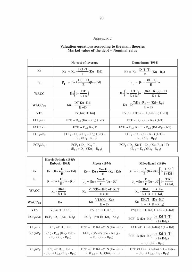
Appendix 2
Valuation equations according to the main theoriesMarket value of the debt = Nominal value
No-cost-of-leverage Damodaran (1994)
Ke
ßL
WACC
WACCBT
VTS PV[Ku; DTKu] PV[Ku; DTKu - D (Kd- RF) (1-T)]
ECFt\\Ku ECFt – Dt-1 (Kut - Kdt) (1-T) ECFt - Dt-1 (Ku - RF ) (1-T)
FCFt\\Ku FCFt + Dt-1 Kut T FCFt + Dt-1 Ku T - Dt-1 (Kd -RF) (1-T)
ECFt\\RF ECFt – Dt-1 (Kut – Kdt) (1-T) – ECFt – Dt-1 (Ku - RF ) (1-T) –– Et-1 (Kut – RF t) – Et-1 (Kut - RF t)
FCFt\\RF FCFt + Dt-1 Kut T – FCFt + Dt-1Ku T - Dt-1(Kd -RF)(1-T) -– (Et-1 + Dt-1)(Kut – RF t) (Et-1 + Dt-1)(Kut - RF t)
Harris-Pringle (1985)Ruback (1995) Myers (1974) Miles-Ezzell (1980)
Ke
ßL
WACC
WACCBT Ku
VTS PV[Ku; T D Kd ] PV[Kd; T D Kd ] PV[Ku; T D Kd] (1+Ku)/(1+Kd)
ECFt\\Ku ECFt - Dt-1 (Kut - Kdt) ECFt - (Vu-E) (Kut - Kd t)
FCFt\\Ku FCFt +T Dt-1 Kdt FCFt +T D Kd +VTS (Ku -Kd) FCF +T D Kd (1+Ku) / (1 + Kd)
ECFt\\RF ECFt - Dt-1 (Kut- Kdt) - ECFt - (Vu-E) (Kut - Kd t) –- Et-1 (Kut - RF t) – Et-1 (Kut - RF t)
– Et-1 (Kut - RF t)
FCFt\\RF FCFt +T D t-1 Kdt - FCFt +T D Kd +VTS (Ku -Kd) FCF +T D Kd (1+Ku) / (1 + Kd) –- (Et-1 + Dt-1)(Kut - RF t) – (Et-1 + Dt-1)(Kut - RF t) – (Et-1 + Dt-1)(Kut - RF t)
20
Ke = Ku +D(1- T)
E(Ku - Kd)
β β β βL
uT
u d = D
E+
−−
( )( )
1
Ku - DT(Ku -
E +D
Kd)
Ke Ku Ku K= +D
E( - d)
β β β βL u u d=D
E+ −( )
Ku -DKdT
E + DKu -
VTS(Ku - Kd) +D KdT
E + D
Ku -VTS(Ku - Kd)
E + DKu -
DKdT
E + D (Ku - Kd)
1( )+ Kd0
ECF - D (Ku - Kd) 1 Kd (1- T)
(1 Kd ) -
0
++
Ku -DKdT
E + D
1 + Ku
1 + Kd0
β β β βL u u d= Vu - E
E+ −( ) β β β βL u u d=
D
E
T Kd
1+Kd+ − −
( ) 1
Ke Ku Ku K= +Vu - E
E ( - d) Ke Ku Ku K= +
D
E ( - d) 1-
T Kd
1+Kd
Ku - DT(Ku - R R
E + DF F) ( )− −Kd
KuDT
E +D1−
Ku
DT
E +D+ D
R
E + DF1
1−
− −( )( )Kd T
β β βL
uT
u = D
E+
−( )1
Ke = Ku +D (1- T)
E (Ku - R )F
ECF - D (Ku - Kd) 1 Kd (1- T)
(1 Kd )0
++

Appendix 2 (continued)
Miller With-cost-of-leverage
Ke
ßL
WACC Ku
WACCBT
VTS 0 PV[Ku; D (KuT+ RF- Kd)]
ECFt\\Ku ECFt - Dt-1 [Kut - Kdt(1-T)] ECFt - Dt-1 [Kut (1-T)+KdtT -RF t]
FCFt\\Ku FCFt FCFt + Dt-1 [Kut T - Kdt + RF t]
ECFt\\RF ECFt - Dt-1 [Kut - Kdt(1-T)] – ECFt - Dt-1 [Kut(1-T)+ KdtT -RF t] – Et-1 (Kut - RF t) – Et-1 (Kut - RF t)
FCFt\\RF FCFt – (Et-1 + Dt-1)(Kut - RF t) FCFt + Dt-1 [Kut T - Kdt + RF t] –– (Et-1 + Dt-1)(Kut - RF t)
Modigliani-Miller Practitioners
Ke
ßL
WACC
WACCBT
VTS PV[RF; T D RF ] PV[Ku; T D Kd - D(Kd- RF)]
ECFt\\Ku ECFt -Dt-1[Kut - Kdt(1-T) -(Ku-g)VTS/D]* ECFt - Dt-1 (Kut - RF t)
FCFt\\Ku FCFt + Et-1 Ku + (Ku-g)VTS * FCFt + Dt-1 [RF t -Kdt (1-T)]
ECFt\\RF ECFt -Dt-1[Kut - Kdt(1-T) -(Ku-g)VTS/D] – ECFt - (Et-1 + Dt-1) (Kut – RF t)– Et-1 (Kut - RF t)*
FCFt\\RF FCFt + Et-1 Ku + (Ku-g)VTS – FCFt + Dt-1 [RF t – Kdt (1-T)] – – (Et-1 + Dt-1)(Kut - RF t)* – (Et-1 + Dt-1) (Kut – RF t)
* Valid only for growing perpetuities.
21
Ke Ku Ku K= +D
E[ d(1- T)]−
β β β βL u u d=D
E
D
E
TKd
PM+ − +( )
Ku +DKd T
E + D
Ke Ku Ku Kd T Ku g VTSD=
D
E*+ − − − −[ ]( ) ( )1
β β β βLM M
= uD
E[ u d
TKd
P-
VTS(Ku - g)
D P]*+ − +
D Ku - (Ku - g) VTS
E + D *
( )
DKu - (Ku - g) VTS + DTKd
E + D*
Ke Ku=D
E (Ku - R )F+
β β βL = uD
Eu+
Ku - DR
E +DF − −Kd T( )1
Ku +DKd - R
E + DF
KuD[(Ku - Kd)T R Kd]
E DF−
+ −+
β β β βL u u T T d=D
E+ − +( ( ) )1
KuD KuT Kd R
E DF−
− ++
( )
Ke Ku Ku= +D
E[ (1- T) +KdT - RF ]

Appendix 2 (continued)
Equations common to all methods:
Relationships between cash flows:
ECFt = FCFt +(Dt-Dt-1)- Dt-1Kdt (1-T) CCFt = FCFt + Dt-1 Kdt T CCFt = ECFt -(Dt-Dt-1)+ Dt-1Kdt
Cash flows\\Ku: ECF\\Ku = ECFt - Et-1 (Ket - Ku t) FCF\\Ku = FCFt - (Et-1 + Dt-1)(WACCt - Ku t) = CCF\\Ku = CCFt - (Et-1 + Dt-1)(WACCBTt - Ku t)
Cash flows\\ RF ECF\\RF = ECFt - Et-1 (Ket - RF t) FCF\\RF = FCFt - (Et-1 + Dt-1)(WACCt - RF t) = CCF\\RF = CCFt - (Et-1 + Dt-1)(WACCBTt - RF t)
ECF\\RF = ECF\\Ku - Et-1 (Kut - RF t) FCF\\RF = FCF\\Ku - (Et-1 + Dt-1)(Kut - RF t) FCF\\Ku - ECF\\Ku = Dt-1 Ku t - (Dt - Dt-1) FCF\\RF - ECF\\RF = Dt-1 RF t - (Dt - Dt-1)
22
WACC = E Ke + D Kd (1- T)
E + Dtt-1 t t-1 t
t-1 t-1( )W =
E Ke + D Kd
E + DBTtt-1 t t-1 t
t-1 t-1ACC
( )

Appendix 3
Valuation equations according to the main theories when the debt’s market value (D) isnot equal to its nominal or book value (N)
This appendix contains the expressions of the basic methods for valuing companiesby discounted cash flows when the debt’s market value (D) is not equal to its nominal value(N). If the debt’s market value (D) is not equal to its nominal value (N), it is because therequired return to debt (Kd) is different from the cost of the debt (r).
The interest paid in a period t is: It = Nt-1 rt . The increase in debt in period t is:∆ Nt = Nt - Nt-1. Consequently, the debt cash flow in period t is: CFd = It - ∆ Nt = Nt-1 rt -(Nt - Nt-1).
Consequently, the value of the debt at t=0 is:
It is easy to show that the relationship between the debt’s market value (D) and itsnominal value (N) is:
Dt - Dt-1 = Nt - Nt-1 + Dt-1 Kdt - Nt-1 rt
Consequently: ∆ Dt = ∆ Nt + Dt-1 Kdt - Nt-1 rt
The fact that the debt’s market value (D) is not equal to its nominal value (N) affectsseveral equations given in section 1 of this paper. Equations [1], [3], [4], [6], [7], [9] and [10]continue to be valid, but the other equations change.
The expression of the WACC in this case is:
[2*]
The expression relating the ECF to the FCF is:
[5*] ECFt = FCFt + (Nt - Nt-1) - Nt-1 rt (1 - T)
The expression relating the CCF to the ECF and the FCF is:
[8*] CCFt = ECFt + CFdt = ECFt - (Nt - Nt-1) + Nt-1 rt = FCFt + Nt-1 rt T
23
D = N r N - N
K0
t-1 t t t-1
t1
tt=1
−
+∏∑∞ ( )
( )1 d
WACC = E Ke + D Kd - N r T
E + D

Appendix (continued)
No-cost-of-leverage Damodaran (1994) Practitioners
WACC
VTS PV[Ku; DTKu + T(Nr-DKd)] PV[Ku; T N r +DT(Ku- RF) - D(Kd- RF)] PV[Ku; T N r - D(Kd- RF)]
FCFt\\Ku FCFt +Dt-1 Kut T + FCFt + Dt-1 Kut T +T(N t-1 rt-D t-1 Kdt) - FCFt +T (N t-1 rt-D t-1 Kdt) ++ T (N t-1 rt-Dt-1 Kdt) - Dt-1 (Kdt - RF t) (1-T) + Dt-1 [RF t -Kdt (1-T)]
Harris-Pringle (1985)Ruback (1995) Myers (1974) Miles-Ezzell (1980)
WACC
VTS PV[Ku; T N r] PV[Kd; T N r ] PV[Kut ; Nt-1 rt T] (1 + Ku) / (1+ Kd)
FCFt\\Ku FCFt +T N t-1 rt FCFt +T N r +VTS (Ku -Kd ) FCF +T N r (1+Ku) / (1 + Kd)
Equations common to all the methods:
WACC and WACCBT:
Relationships between the cash flows:
24
Ku - N rT +DT(Ku -
E +D
Kd)
( )Ku -
N rT +D[T(Ku - R R
E + DF F) ( )]
( )
− −KdKu -
N rT - D R
E +DF( )
( )
Kd −
Ku -N rT
E +D( ) Ku -VTS(Ku - Kd) +N rT
E + D( )Ku - N
r T
E + D 1 + Ku
1 + Kd( )
W = E Ke + D Kd - N r T
E + Dtt-1 t t-1 t t-1 t
t-1 t-1ACC
( )
W = E Ke + D Kd
E + DBTtt-1 t t-1 t
t-1 t-1ACC
( )
W - W = N r T
E + DBTt tt-1 t
t-1 t-1ACC ACC
( )
ECF = FCF (N - N ) - N r (1- T)t t t t-1 t-1 t+
CCF = ECF - (N - N ) +N rt t t t-1 t-1 t
CCF CF rt t t-1 t = F +N T

Appendix 4
Dictionary
βd = Beta of debt βL = Beta of levered equityβu = Beta of unlevered equity = beta of assets D = Value of debt E = Value of equityEbv = Book value of equityECF = Equity cash flow EP = Economic ProfitEVA = Economic value addedFCF = Free cash flowg = Growth rate of the constant growth case I = Interest paid Ku = Cost of unlevered equity (required return to unlevered equity) Ke = Cost of levered equity (required return to levered equity)Kd = Required return to debt = cost of debt N = Book value of the debtNOPAT = Net Operating Profit After Tax = profit after tax of the unlevered companyPAT = Profit after tax PBT = Profit before tax PM = Market premium = E (RM - RF)PV = Present valuer = Cost of debtRF = Risk-free rateT = Corporate tax rateVTS = Value of the tax shieldVu = Value of shares in the unlevered companyWACC = Weighted average cost of capitalWACCBT = Weighted average cost of capital before taxesWCR = Working capital requirements = net current assets
25

References
Arditti, F.D. and H. Levy (1977). “The Weighted Average Cost of Capital as a Cutoff Rate: ACritical Examination of the Classical Textbook Weighted Average”, FinancialManagement (Fall), pp. 24-34.
Copeland, T.E., T. Koller and J. Murrin (2000). Valuation: Measuring and Managing theValue of Companies. Third edition. New York: Wiley.
Damodaran, A (1994). Damodaran on Valuation, John Wiley and Sons, New York.
Fernández, Pablo (2002). Valuation Methods and Shareholder Value Creation, AcademicPress.
Fernández, Pablo (2004). “The value of tax shields is NOT equal to the present value of taxshields”, Forthcoming in the Journal of Financial Economics.
Fernández, Pablo (2004). “The Value of Tax Shields and the Risk of the Net Increase ofDebt”, SSRN Working Paper no. 506005.
Harris, R.S. and J.J. Pringle (1985). “Risk-Adjusted Discount Rates: Transition from theAverage-Risk Case”, Journal of Financial Research (Fall), pp. 237-244.
Inselbag, I. and H. Kaufold (1997). “Two DCF Approaches for Valuing Companies underAlternative Financing Strategies (and How to Choose Between Them)”, Journal ofApplied Corporate Finance (Spring), pp. 114-122.
Kaplan, Steven and Richard Ruback (1995). “The Valuation of Cash Flow Forecasts: AnEmpirical Analysis”, Journal of Finance, Vol 50, No 4, September.
Lewellen, W.G. and D.R. Emery (1986). “Corporate Debt Management and the Value of theFirm”, Journal of Financial Quantitative Analysis (December), pp. 415-426.
Luehrman, Timothy A. (1997). “What’s It Worth: A General Manager’s Guide to Valuation”,and “Using APV: A Better Tool for Valuing Operations”, Harvard Business Review,(May-June), pp. 132-154.
Miles, J.A. and J.R. Ezzell (1980). “The Weighted Average Cost of Capital, Perfect CapitalMarkets and Project Life: A Clarification,” Journal of Financial and QuantitativeAnalysis (September), pp. 719-730.
Miles, J.A. and J.R. Ezzell, (1985). “Reequationing Tax Shield Valuation: A Note”, Journalof Finance, Vol XL, 5 (December), pp. 1485-1492.
Miller, Merton H. (1977).“Debt and Taxes”, Journal of Finance (May), pp. 261-276.
Modigliani, Franco, and Merton Miller (1958). “The Cost of Capital, Corporation Financeand the Theory of Investment”, American Economic Review 48, 261-297.
Modigliani, Franco and Merton Miller (1963). “Corporate Income Taxes and the Cost ofCapital: A Correction”, American Economic Review (June), pp. 433-443.
26

Myers, S.C. (1974). “Interactions of Corporate Financing and Investment Decisions -Implications for Capital Budgeting”, Journal of Finance (March), pp. 1-25
Ruback, Richard S. (1995). “A Note on Capital Cash Flow Valuation”, Harvard BusinessSchool, 9-295-069.
Tham, Joseph and Ignacio Vélez-Pareja (2001). “The correct discount rate for the tax shield:the N-period case”, SSRN Working Paper.
27