FINANCE DISCIPLINE GROUP fileprices fall by 3.9% for homes within 0.2 miles of the ... rental data...

FINANCE DISCIPLINE GROUP

UTS BUSINESS SCHOOL

WORKING PAPER NO.181 March 2014

Does a Nearby Murder Affect Housing Prices and Rents? The Case of Sydney Anastasia Klimova Adrian D. Lee

ISSN: 1837-1221 http://www.business.uts.edu.au/finance/

1

Does a Nearby Murder Affect Housing Prices and Rents? The Case of

Sydney*

Anastasia Klimova

Adrian D. Lee

Economic Record, Accepted

Latest Draft: 16th March 2014

Abstract

We measure the impact of murders on prices and rents of homes in Sydney. We find that housing prices fall by 3.9% for homes within 0.2 miles of the murder, in the year following the murder, and weaker results in the second year after a murder. We do not find any effects of murders on rents. Higher media coverage and being located closer to the murder (within 0.1 mile) have no additional effect on prices. Taken together, our findings suggest that proximity to a murder affects nearby property prices, particularly in the first year after the incident.

Keywords: Crime, murder, homicide, house prices, rent, hedonic model

JEL Classification: G14, K32, Q51, R2

* The paper has benefited from comments and suggestions by Susumu Imai, Meliyanni Johar, Jinu Kim, Daniel Melser, Gary Painter, Olena Stavrunova and conference participants at the 2012 American Real Estate and Urban Economics Association International Conference. We thank Australian Property Monitors for the provision of the house price and rental data and acknowledge funding from the UTS Business School Research Grant. Economics Discipline Group, University of Technology, Sydney, Sydney NSW 2000 Australia. Finance Discipline Group, University of Technology, Sydney, Sydney NSW 2000 Australia.

2

1. Introduction

Homes stigmatized by traumatic events such as a murder or a suicide are well known to

sell at deep discounts and to take longer to sell. However, there has been no research on

whether a traumatic event near a home affects its price or rent. This question is pertinent for

two reasons. Firstly, the magnitude of the spillover effect of the trauma onto the immediate

area, as an unnatural death signals to existing and prospective homeowners of disamenities in

the area, which may not have been so evident previously. Secondly, unnatural deaths, such as

a murder, are usually only disclosed to the public by news media following police reports and

so there would be search costs involved for the buyer to uncover such disamenities. Also,

while in many US jurisdictions real estate agents are required to disclose stigmatized features

of a particular home, it is not clear to what extent one needs to disclose nearby murders and

other ill occurrences. Buyers and renters may therefore be unaware of the stigmatized

features of a property.

This paper attempts to measure the effect of murders on housing prices and rents in

Sydney, the largest and most populous city in Australia, from 2003 to 2010. In contrast to the

US, Australia experienced an economic and housing boom throughout this period with no

large decreases in prices during the global financial crisis in 2008. The murder rate during the

data period was quite low, on average 1.31 victims per 100,000 in Sydney, and exhibited a

downward trend. The low murder rate and reasonable geographic spread of murders across

Sydney allow an analysis of the impact across very small regions and specific points in time

without other confounding effects.

This paper contributes to a growing literature on house prices and the fear of crime.

We follow in the same vein of literature on disamenity risks such as a sex offender moving

into a neighbourhood (e.g. Linden and Rockoff (2008); Pope (2008); Wentland, Waller et al.

3

(2013)) and the discovery of a methamphetamine laboratory (meth lab) (e.g. Congdon-

Hohman (2012)). These papers find that prices fall between 4% to 10% after the impact of

the disamenity (an arrival of a sex offender or a discovery of a meth lab). These papers avoid

typical endogeneity issues with crime and house prices1 by assuming the arrival or discovery

of a disamenity is random for a very small geographic region (e.g. within 0.25 to 0.3 miles

from it). For example, Linden and Rockoff (2008) estimate individuals’ valuation of living in

close proximity to a convicted sex offender by exploiting both intertemporal and cross-

sectional variance in the presence of an offender, and Pope (2008) observes not only the

arrivals of offenders in the neighbourhoods but their departures as well. All these studies find

that the presence of offenders causes a 4% to 10% reduction in the sale price of homes within

0.1 miles of the disamenity. Unlike this paper, however, previous studies make use of

databases publicly available from either county departments or the police, which makes

search costs low for buyers.

This paper also contributes to a larger body of literature investigating the impact of

crime on house prices spanning decades, starting from papers by Thaler (1978) and Hellman

and Naroff (1979). A more recent paper by Pope and Pope (2012) examines the relationship

between changes in crime rates and property prices during the nationwide decrease in crime

in the USA in 1990s. They find a strong relationship between crime and property values

during that time. However, the impact of the cost of crime on house prices is not uniform

throughout the market (Lynch and Rasmussen (2001), Ihlanfeldt and Mayock (2010)) and

often depends on the type of crime. When weighing the seriousness of offences by the cost of

crime to victims instead of the customary measures of the number of index crimes, Lynch and

Rasmussen (2001) find that the cost of crime has almost no impact on house prices overall;

however, homes are highly discounted in high crime areas. By investigating the relationship

1 Ihlanfeldt, K. and T. Mayock (2010) p. 162 provides a summary of the potential endogeneity issues.

4

between different crime types and house prices, Gibbons (2004) finds that crimes in the

criminal damage category (e.g. vandalism, graffiti) have a significant negative impact on

prices, while burglaries have no measurable impact on prices. While most papers focus on a

single type of crime, Ihlanfeldt and Mayock (2010) study the effect of various types of crime

on housing prices and find that of their seven different categories of crime only robbery and

aggravated assault crimes had a significant impact on housing values.

Moreover, this paper contributes to the limited literature on the relationship between

crime and residential property rents. Some studies of the effect of crime on rents find the

relationship to be negative. For example, Ozanne and Malpezzi (1985) find that crime

decreased rents in Pittsburgh and Phoenix in 1974. In his study of rents, Rizzo (1979)

estimated an elasticity of an overall crime measure with respect to rents of -0.24 in Chicago

in 1970 (or -0.15 when controlling for the income, which he explained by low quality

housing being confounded with high crime rates in its effect on rents) (p.18).

Another valuable contribution of this paper is the unique data set that we use to

analyse the effect of murders on property prices. We collected a vast amount of information

on murders in Sydney between 2003 and 2010. From the official statistics we obtained the

number of murder victims by month and area and then manually matched each victim with

details of each murder, using an array of sources ranging from news articles to police media

releases and court decisions.

Using a merged database of murders, with housing prices and rents in Sydney, we

find that housing prices within 0.2 miles and one year of a murder fall by 3.9%. High media

coverage and being closer (within 0.1 miles) to a murder have no additional effect on prices,

suggesting that murders have no localized effect. We also find no effect on rents, and weaker

results when using a longer, two-year window. Taken together, our findings suggest that

5

proximity to a murder affects nearby housing prices, particularly in the first year after the

incident.

This paper proceeds as follows: section 2 provides background on murders and house

prices in Sydney; then we develop hypotheses in section 3, followed by a description of the

data in section 4; section 5 describes the methodology, section 6 reports our results and

section 7 concludes.

2. Murders in Sydney

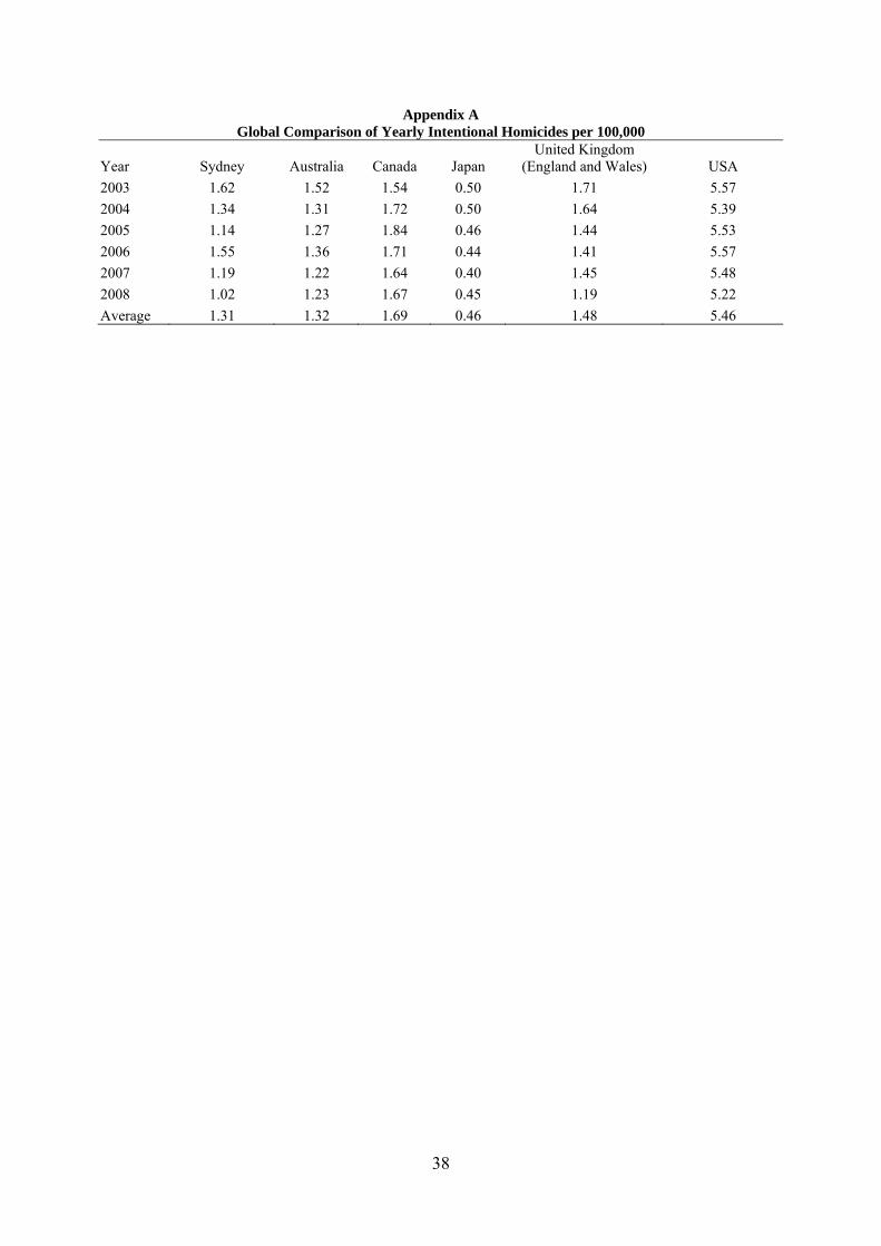
The rate of murder in Sydney is similar to that of Australia as a whole and reasonably

low in comparison to the world. Appendix A reports yearly intentional homicide rates per

100,000 people for Sydney, Australia, Canada, Japan, United Kingdom and the United States

from 2003 to 2008. Statistics for Sydney are compiled from NSW Bureau of Crime Statistics

and Research (BOCSAR) murder victim statistics and Australian Bureau of Statistics Sydney

population statistics. Country murder rates are taken from the UN data website.2 Overall, all

countries have experienced falling or stable murder rates over the period. Sydney has also

experienced a reduction in murder rates from 1.62 per 100,000 in 2003 to 1.02 in 2008. On

average, the murder rate in Sydney is 1.31, which is second only to Japan in the sample of the

countries. This is despite Sydney being the most populous and densely populated city in

Australia, with about 5,849 people per square mile in 2009. The low murder rate and large

size of Sydney, therefore, allow us to study house prices before and after the event of a

murder in a specific location.

Murders in Sydney are often reported in the large city newspapers or local

newspapers, due to their rarity and shocking nature for Sydneysiders. Since 2004, both state

2 http://data.un.org/Data.aspx?d=UNODC&f=tableCode%3A1.

6

legislation and case law3 require real estate agents to disclose whether a murder has occurred

in a house. The law was introduced after a real estate agent failed to disclose a triple murder

that had occurred in a house, with the buyer only realising the home's history after paying a

deposit. The law, however, does not require agents to provide information on nearby

murders. There are even fewer disclosure requirements for rental agreements, suggesting that

rental tenants may suffer even higher search costs for disamenities.

3. Hypothesis Development

In a market where homeowners and renters are fully informed of murders, there are two

ways in which a murder may affect nearby housing prices and rents. Firstly, homes where a

murder has been committed clearly sell at a discount and so arguably nearby homes might

also be discounted due to the stigma of living near these homes. Secondly, a nearby murder

may also be considered a disamenity as it brings psychological anxiety and stress to

neighbours. For example, Sharkey (2010) finds that African-American children in Chicago

neighbourhoods have statistically lower vocabulary and reading assessment scores if a

murder occurs in their block group less than a week before the assessment task. While the

findings of Sharkey (2010) are short-term, they nonetheless show that the effect of murder on

nearby residents is non-trivial. Our first hypothesis is therefore:

H1: Homes closer to a murder location have greater price falls than those slightly further

away.

Murders, however, are not always fully disclosed, and buyers and renters require

much research to uncover such disamenities. Sellers, on the other hand, would have better

3 See Property, Stock and Business Agents Act 2002 (NSW) s 52 and Hinton & Ors v. Commissioner of Fair Trading, NSWADT, 2006.

7

knowledge of a nearby murder through community word of mouth, closer attention to media

about the local area and police doorknocking. It is possible that extensive media coverage can

reduce such information asymmetry. However, a by-product of such coverage is a possible

sensationalisation of the murder, increasing the fear of crime in the local area (e.g. Ditton and

Duffy (1983), Smith (1984) and Williams and Dickinson (1993)). Such an increased fear of

crime may depress prices more in the area than if the murder was unreported or only reported

locally. This, therefore, provides us with our second hypothesis:

H2: Murders with high media coverage lead to greater price falls than those with low media

coverage.

4. Data

We use two datasets in our analysis of the effects of murder on house prices and rent.

The first source is the NSW BOCSAR recorded crime dataset. The data is available freely

from the BOCSAR website4. The dataset is derived from police incident reports and

recorded on the NSW Police Force's Computerised Operation Policing System (COPS). It

provides monthly crime statistics including the offence type, number of each offence (or

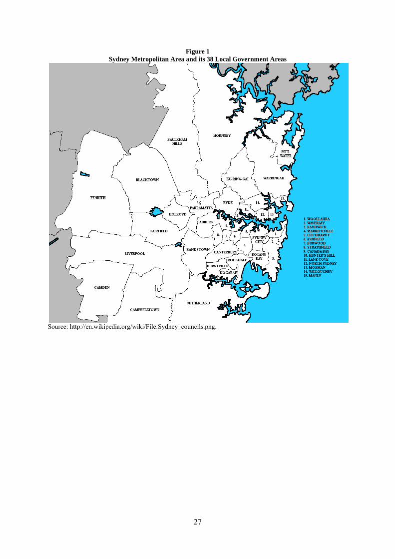
victims in the case of murder or manslaughter) in a Local Government Area (LGA). Each

LGA covers many suburbs, with Sydney containing 38 LGAs. A map of the 38 LGAs of

Sydney is found in Figure 1.

From the recorded crime dataset, we take the monthly number of murder victims in

each Sydney LGA. We choose murder instead of manslaughter as a murder is more likely to

be announced through news media due to its severity and infrequency. With the murder

victims by month and LGA, we then manually match each victim with details of each murder

4 http://www.bocsar.nsw.gov.au/lawlink/bocsar/ll_bocsar.nsf/pages/bocsar_research.

8

through articles from the NSW Police media releases5, court decisions6 and local, city or

national newspapers via Factiva and/or their web pages from 2005 to 2009. We use this

sample period as we require two years of sales data before and after a murder and we have

house sales and rental data from 2003 to 2011. Using the sources of information mentioned

above, we compiled data to add to the BOCSAR statistics, including information on the date

when the murder occurred, and a suburb and a street where murder victim(s) were found. If

the exact location is not found we look for information that can bring us closer to the location

of a murder event. For example, a news article may state that a murder occurred at a home

near a certain intersection or at a commercial venue. We then make use of past ownership

records from the Australian Property Monitors web database (www.apmpropertydata.com.au)

and if a photo is shown in a news article, use Google map's 'street view' function to locate the

exact address. We then geocode the location if the exact address is known or use the middle

of the street if we do not have the exact location of the murder.

Appendix B provides details on the number of murder victims reported by BOCSAR

and those that we are able to identify and/or geocode accurately by year of murder from 2003

to 2010.7 We define an accurately geocoded murder as if we have the exact location of the

murder or if a 0.1 miles radius covers the entire street where the murder occurred. In total

from 2003 to 2010, we were able to find articles related to 327 of the 386 victims and

accurately geocode 273 of the 386 murder victims reported by BOCSAR or almost 71%. Our

success at geocoding locations ranges from 62% of murders in 2004 to 80% of murders in

2009. This compares reasonably to Linden and Rockoff (2008) and Pope (2008) who match

5 http://www.police.nsw.gov.au/news/media_release_archives. Additional media releases are found using the Internet Archive website (http://www.archive.org/web/web.php) which captures the website at various points in time. Police media releases are also released through the Australian Associated Press (AAP). 6 http://www.austlii.edu.au and mainly decisions from the Supreme Court of New South Wales or the Supreme Court of New South Wales - Court of Criminal Appeal. 7 While we only investigate murders from 2005 to 2009, we collect murders from 2003 to 2004 and 2010 to ensure the effects we find are not driven by murders prior to or after our sample period.

9

87% and 85% of sex offenders to an address in their datasets respectively. Of the 54 victims

which we find articles for but could not accurately geocode, 47 was because of a lack of

information in articles and seven were murder charges where the body was found elsewhere

or not found at all. In all we analyse 175 unique murder locations from 2005 to 2009.

Figure 2 plots the location of each murder within suburbs across LGAs. Murders

cluster within Inner Sydney although for a majority of murders there is a reasonable

geographical spread.

Table 1 reports summary statistics for the number of newspaper articles during the

month after a murder in Panel A; a cause of death and a number of media articles in Panel B,

and a location of the murder and a number of media articles in Panel C.

We find that most murders that we classify as having location data are reported in at

least one newspaper with only 24 murders not having the location of the murder reported

(See Table 1 Panel A). The Daily Telegraph also reports more murders than the Sydney

Morning Herald consistent with tabloids reporting more on crime than broadsheets as

Williams and Dickinson (1993) find.

The most common murder is a stabbing, accounting for 42.5% of murders followed

by shootings at around 22%. Perhaps due to its unusual nature, shootings also attract more

media articles (mean of 3.69 articles per shooting murder) in comparison to stabbings (mean

of 2.22) (See Table 1 Panel B). Finally, data shows that a home (house, apartment or other

housing type) is the most common place for a murder representing 57% of murders. Street

murders make up just over 21% while other locations such as commercial venues,

recreational areas and other public places make up the remainder. Murders at public places

such as parks, petrol stations, pubs and shopping malls also attract more newspaper articles

on average than homes except for apartments where the mean number of articles is 4.03 (See

Table 1 Panel C).

10

Our second data source is from Australian Property Monitors (APM) which contains

house sales and rental listings for the Sydney metropolitan area. The sales data contains the

sales price and contract date from 2003 to 2011 while the rental listings come from a major

internet listing service and contain the advertised weekly rental price and listing dates from

2003 to 2011. Both datasets also record characteristics of the homes including the property

type (home or unit/condominium), the number of bedrooms and bathrooms, the size of the

house8 and whether the home has more than one parking spot. The data also contains an

extensive list of ‘additional’ housing characteristics which include the types of rooms that the

home has (e.g. balcony, separate dining, family room, sunroom, rumpus room, etc.); home

comforts (e.g. air conditioning, heating, sauna, spa, pool, etc.) and views (e.g. water, harbour,

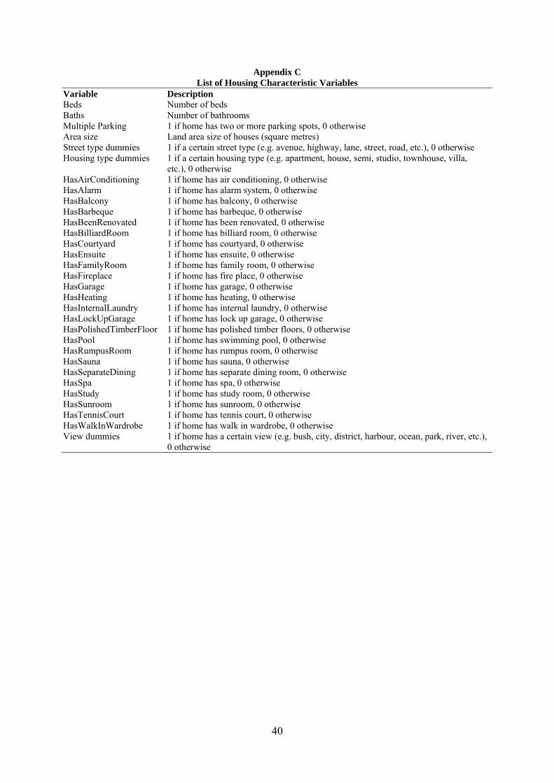
ocean, district views etc.). Appendix C details the list of housing characteristics’ variables

that we use. For rental listings, we use the last advertised rental price of the property. We also

filter out home sales prices and rents which have incomplete data. Prices and rents are also

standardised to 2011 dollars using the consumer price index as per the methodology of

Linden and Rockoff (2008).

We then match murder locations to sales and rental properties which occur within 0.3

miles radius of a murder location and one year before or after the murder. The use of 0.3

miles is the same boundary that Linden and Rockoff (2008) and Pope (2008) use for sex

offender locations. Linden and Rockoff (2008) p.1106 state that their choice of 0.3 miles is

based on the Louisiana law requiring sex offenders to inform all neighbours living within this

distance from their home of their presence. As there is no such a law for murders, in Section

6.1 we consider the feasibility of using different distances.

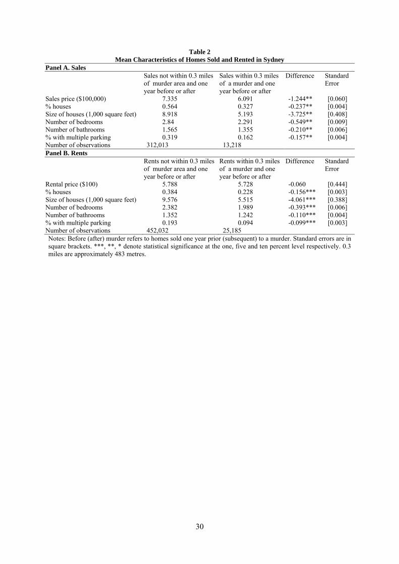
Table 2 reports average housing characteristics for our housing sales data in Panel A

and rental listings in Panel B. Column 1 of both Panels reports for not within 0.3 miles of a

8 Unfortunately, the floor space of each unit is not provided.

11

murder location and column 2 reports for homes within 0.3 miles of a murder location. As

can be seen, on average, areas near murders have fewer houses and properties in those areas

have fewer bedrooms, bathrooms, less parking, and sell at lower prices. Our findings are

consistent with the literature on crime and house prices which finds that criminal activity

tends to occur in cheaper neighbourhoods (e.g. Ihlanfeldt and Mayock (2010); Congdon-

Hohman (2012)). While this may suggest an endogeneity problem between housing prices

and rents with murders, we hope to overcome this by assuming murders are random within

the 0.3 mile region of a murder and by comparing homes within 0.1 and 0.2 miles of the

murder to homes between 0.2 and 0.3 miles away as we describe below.

5. Methodology

In order to test whether murders affect house prices, we apply the 'difference-in-

difference' hedonic model methodology that Linden and Rockoff (2008) and Pope (2008) use.

The basis of the difference-in-difference approach is that homes near the murder are similar

in characteristics to homes slightly further away from the murder.

Following Linden and Rockoff (2008) in the first stage, we compare whether there are

any statistical differences in housing prices and rents for homes within 0.1 or 0.2 miles from a

murder (the treatment groups) and between 0.2 and 0.3 miles (the control group) from the

murder and one year prior to the murder. For the difference-in-difference test to work, prices

and rents of homes within 0.1 or 0.2 miles of a murder must not be statistically different from

those of homes slightly further away, between 0.2 and 0.3 miles away9. Statistical difference

would suggest that our control variables cannot adequately account for spatial heterogeneity

within murder locations due to some unobservable variables. For example, if murders tended

to occur in known crime hotspots, this may make prices lower in the 0.1 mile radius despite

9 The use of miles instead of metres is by convention in difference-in-difference studies for housing prices. 0.3, 0.2 and 0.1 miles is approximately 483, 322 and 161 metres, respectively.

12

controlling for all known housing characteristics. The test will also reveal whether wider (or

narrower) samples may be chosen due to the degree of hetereogeneity in the control and

treatment groups.

Formally, we apply the following regression for all homes within 0.3 miles of a murder

and one year prior to the murder which is similar to equation 1 from Linden and Rockoff

(2008) except for the inclusion of a 0.2 mile dummy variable. We include a 0.2 mile dummy

variable following Pope (2008) to test whether there is an effect for slightly further distances

from the murder. The regression we use is:

log 1

110

2

210 , (1)

where i,r,t subscript for the home, murder area and contract date respectively. log is the

log price or rent of a home. is the intercept with year fixed effects. We also substitute the

dependent variable with a dummy variable of 1 for whether the home is a house (or 0

otherwise), size of houses (in 1,000 square feet), number of bedrooms, number of bathrooms

and a dummy variable of 1 for whether the home has multiple parking spots. / is a

dummy variable with a value of 1 if a home is within 0.1 miles from a murder and 0

otherwise. / is a dummy variable with a value of 1 if a home is between 0.1 and 0.2

miles from a murder and 0 otherwise. Standard errors clustered10 by the location of the

murder are used following Linden and Rockoff (2008). We also apply the regression to our

rental listings database.

In the second stage, we formally test whether murders affect the prices and rents of

homes by applying the following regression to homes within 0.2 miles and homes within 0.3

miles of a murder:

10 These are White, H. (1980) standard errors adjusted to account for possible within cluster correlation. See Petersen, M. A. (2009) for more detail on clustered standard errors.

13

(2)

where are the year/quarter and murder area fixed effects, are our c housing

characteristic measures. time is a factor to control for linear time trends specific to the

murder area while time2 takes into account quadratic time trends. / is a dummy variable

with the value of 1 if a home is between 0.2 and 0.3 miles from a murder and one year before

or one year after the murder and 0 otherwise. is a dummy variable if the sale or

rental listing occurs between one month to one year after the murder. We exclude one month

after the murder to allow for information about the murder to have spread to buyers and

sellers. When we extend our analysis to the full sample of sales or rental listings, we use

suburb fixed effects instead of murder area fixed effects and suburb linear time trend.

For rental listings, we substitute the dependent variable with log of the weekly rental

price. If murders had an impact on house prices or rents, the coefficient or would be

negative and statistically significant.

We also extend the basic difference-in-difference model to test our hypothesis on

media coverage. To test the high media hypothesis, we create an interaction variable mediart

with a value of 1 if there are more than two articles in the two major Sydney newspapers, The

Sydney Morning Herald and The Daily Telegraph in the first month following the murder

which reveal the location of the murder, and 0 otherwise. We use more than two articles to

define a murder with high media coverage, as the median number of articles for all murders is

two. We interact media with the / , / and / and dummy variables. If the

coefficients for / × ×mediart, / × ×mediart and / × ×mediart

14

are negative and statistically significant then this suggests that houses near murders that had

high media exposure had larger price falls for homes within 0.1 miles, between 0.1 and 0.2

miles and between 0.2 and 0.3 miles respectively, than those that did not.

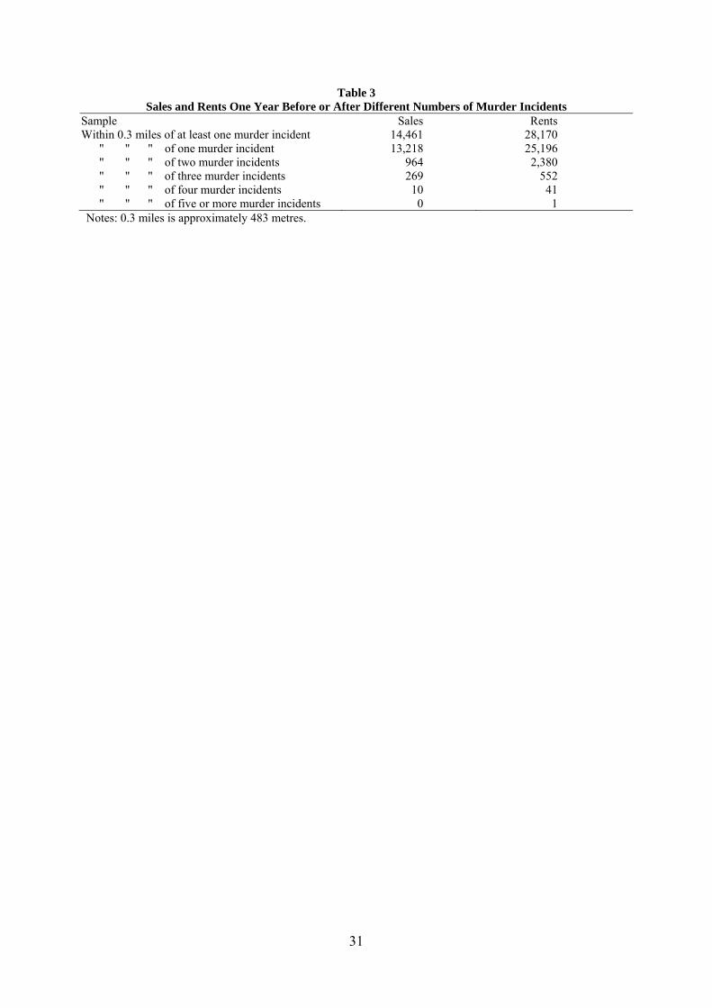
Following Pope (2008), an area where a murder occurred is defined within 0.3 miles

of only one murder and either one year before or after it. The homes within 0.3 miles of more

than one murder are excluded from the murder location samples. The purpose of this

classification is to ensure the homes studied are not affected by other murders which may

lead to ambiguous results. For example, if a home sale occurs before one murder and also

occurs immediately after another one then it is difficult to assign it to either a treatment (after

a murder) or non-treatment group (before a murder or between 0.2 and 0.3 miles of a

murder).

We also only analyse the effect of murders which locations were geocoded with

accuracy as per Appendix B. We make use of accurate locations so that we can also

investigate whether being very close to the murder location (e.g. next to the murder or a few

doors away) affects housing prices and rents.

Table 3 reports the extent to which these filters affect our sample. We find that the

majority of sales (13,218 or above 91%) and rental listings (25,196 or above 89%) within at

least one murder incident are affected by only one murder. As such the majority of homes

within 0.3 miles and one year before or after were exposed to only one murder.

6. Results

6.1 Homogeneity of Homes within 0.3 Miles of a Murder

For our difference-in-difference hedonic model to produce reliable results, homes

within 0.1 or 0.2 miles must be reasonably homogenous compared with homes between 0.2

and 0.3 miles from a murder.

15

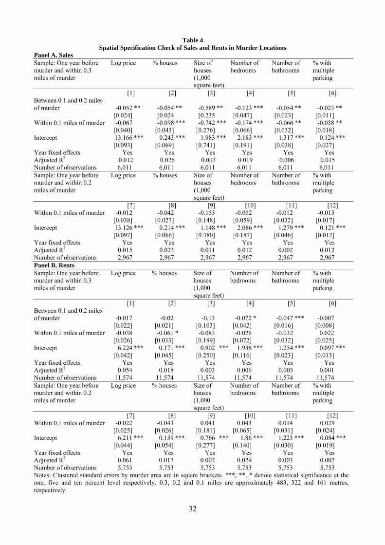
Table 4 Panel A estimates equation 1 using home sales across housing characteristics

from columns 1 to 6 and a sample of sales one year before a murder and within 0.3 miles of a

murder. The results show that there is a statistically significant difference in housing

characteristics of the treatment groups to the control groups, with the treatment group homes

being cheaper and smaller.11 For example, sale prices of homes within 0.1 miles of a murder

are 6.7% lower than those of homes between 0.2 and 0.3 miles. Moreover, within 0.1 miles

there are 9.8% fewer houses, and they are on average 742 square feet smaller, with fewer

bedrooms, bathrooms and parking spaces than those further away. Similar results are found

for homes between 0.1 and 0.2 miles of a murder.

The hetereogeneity between areas suggests that home between 0.2 and 0.3 miles

potentially do not make a good control group as there may be some unobserved

characteristics that we cannot control for. This also means that we are unable to use homes

further than 0.3 miles (e.g. homes between 0.3 and 0.5 miles) due to the hetereogeneity of

areas. Consequently, we consider using homes closer to the murder, between 0.1 and 0.2

miles as a control (Table 4 Panel A columns 7 to 12) and find there is no statistical difference

between the two samples. As such, in our second stage regressions, we consider using both

the 0.3 mile and 0.2 miles samples for robustness. For our rental sample (Table 4 Panel B),

we find little statistical difference between the control and treatment groups.

6.2 Effect of Nearby Murders on Housing Prices and Rents

This section reports our baseline estimates of equation 2 for sales and rental listings.

Noting potential omitted variables issues as found in the above section, we use different

specifications of equation 2. As shown in Table 5, we find evidence of house prices within a

11 Using fixed effects for areas close to a murder does not reduce the statistical differences in characteristics that we find.

16

0.2 mile radius of and up to one year after a murder falling by between 3.8% to 5.0%,

although no change in rents was observed.

On our basic model for housing prices, using the full sample in column 1 (similar to

the specification of Linden and Rockoff (2008)’s Table 3 column 4)12, we find no statistical

difference in prices for homes within 0.1 miles of a murder or between 0.1 and 0.2 miles to

those between 0.2 and 0.3 miles away, as evident by the coefficients for 'Within 0.1 miles of

murder' and 'Between 0.1 and 0.2 miles of murder' variables. This suggests that the inclusion

of housing characteristics, fixed effects and time trends helps explain the price differences

that we found in Table 4 Panel A. For our treatment samples, the coefficients of 'Within 0.1

miles of murder × after' and 'Between 0.1 and 0.2 miles of murder × after' variables are

negative but not statistically significant, suggesting that prices of houses closest to a murder

do not differ from those only slightly further away.

In column 2, where we constrain the sample to only sales one year before or after a

murder and within 0.3 miles of a murder, we find the coefficients of 'Between 0.1 and 0.2

miles of murder × after' and 'Within 0.1 miles of murder × after' variables are -0.033 and -

0.032 respectively and statistically significant.

To correctly estimate the percentage impact of a dummy variable on the level of the

dependent variable in semilogarithmic regression equations, we follow Kennedy’s approach13

(Goldberger (1968), Halvorsen and Palmquist (1980), Kennedy (1981)). The approximate

unbiased estimator of the percentage change in price or rent due to change in our dummy

variables is given by p 100 exp c 12V c 1 (Kennedy (1981)). Applying this

12 We only use suburb time trends and not suburb quadratic time trends for the full sample due to computational constraints. 13van Garderen and Shah (2002) derive an exact unbiased estimator, and after applying to teacher earnings, they find that ‘Kennedy’s estimates are practically indistinguishable from the exact unbiased ones” (p. 153). They explain that the estimates are expected to be close. Therefore, we choose Kennedy’s approach in our study.

17

formula, we find that housing prices after a murder fall by about 3.9 %. The 3.9% is an

economically significant amount and is comparable to the fall in housing prices caused by

proximity of sex offenders as in Linden and Rockoff (2008) (4.1%) and Pope (2008) (2.3%),

except the affected area in latter studies is only within 0.1 miles. If we consider that a home

one year prior and within 0.2 miles of a murder was worth14 about exp(13.13) ≈ $504,000,

then the loss from a negative effect of a nearby murder is about $19,600 (USD$15,70015) per

home. As such, the fall in dollar terms from a murder is more than twice as large as that

estimated by Linden and Rockoff (2008), of USD$5,500 for sex offenders moving into

Mecklenberg County. If we make a further conservative estimate that there are about 60

homes within 0.2 miles of a murder, then each murder causes about $1,176,000 in price falls.

In column 3, where we further constrain the sample to only homes within 0.2 miles,

thereby ensuring homes are homogenous in the control and treatment areas, we find

statistically significant and larger estimates of the coefficients of -0.037 and -0.042

respectively. Our findings suggest that using only sample of houses that were located closer

to a murder reduces noise in our estimates, consistent with Linden and Rockoff (2008)'s

results that are more statistically significant when using their 0.3 mile sample.

In order to test whether distance from a murder location affects pricing, column 4 uses

a variable for the linear distance from the murder for sales within 0.1 miles of the murder,

following Linden and Rockoff (2008)'s Table 3 column 6 methodology. The variable is

scaled such that 0.1 miles = 1. The coefficient for this variable 'Dist≤ 0.1 miles × after' is

statistically insignificant, suggesting that prices of homes closer to the murder area do not fall

14 Using the intercept coefficient estimate for Table 4 Panel A column 7 for the within 0.2 mile sample as the average log price. 15 Using an average monthly AUD/USD rate of 0.80 across our sample period.

18

more after the murder than those further away. This is consistent with the findings in columns

2 and 3 where both 0.2 and 0.1 mile dummy variables have similar coefficients.

Our rental results in columns 5 to 8 show no statistical significance for the 'after'

coefficients, suggesting that murders have no effect on rental prices.

6.3 Reconciliation of Full Sample and Murder Area Results

Our results in section 6.2 and Table 5 for full sample versus 0.3 and 0.2 mile samples

appear inconsistent prima facie as the coefficient of the variables of the full sample while

being negative are not statistically different from zero. It therefore appears that we have

picked the 0.3 and 0.2 miles since we have statistically significant results.16

A possible reason for these results is that we do not use a reasonable hedonic model

for our regressions. We have used all variables at our disposal though there is a chance that

we have overfitted the model which might have increased noise in our coefficient estimates.

As such we estimate various hedonic models and report selection criteria to test whether our

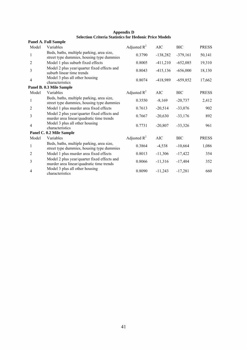
full model is the best fit for our samples. We report our results in Appendix D. Appendix D

Panel A reports several models using the full sample starting with Model 1 that uses the least

number of independent variables (only beds, baths, multiple parking, area size, street type

dummies, housing type dummies which are common hedonic pricing variables used in the

literature). The final Model 4 in Panel A includes all variables that we use in our baseline

results. All our selection criteria adjusted R2, Akaike information criteria (AIC), Bayesian

information criteria (BIC) and predicted residual sums of squares (PRESS) show that Model

4 is superior indicating we have used the best possible model in our baseline regressions.

Appendix D Panel B and Panel C report results for the 0.3 mile and 0.2 mile sample

respectively which show that while adjusted R2 is highest for Model 4, Model 3 (without

16 We thank the referee for this helpful suggestion.

19

additional housing characteristics) has the lowest score for AIC, BIC and PRESS. In

unreported results, we re-estimate our Table 5 baseline results without the additional housing

characteristics and find qualitatively similar results. As such it does not appear the poor fit of

our model is the reason for the inconsistent results.

Another possible reason for the lack of statistical significance is as Linden and

Rockoff (2008) p.1,117 note when using full sample analysis that there 'is the assumption that

the relationship between housing characteristics and prices outside of the offender areas are

valuable in estimating the relationship between characteristics and prices within the offender

areas.' They then go on to use only offender areas to estimate their results. Indeed Congdon-

Hohman (2013)'s baseline results in Table 4 for meth labs also find negative insignificant

result for the full sample and negative and statistically significant results for the within area

results. He reasons that this is in part due to differences in hedonic valuations within the full

sample and the within area results. As such, a simple method of reconciling our full sample

and within area results is therefore to use murder area dummies to control for differences in

characteristics in the full sample results.

Appendix E reports our results for full sample regressions using murder area fixed

effects. Areas not within our murder areas are placed in their own area. Column 1 reports

results with murder area fixed effects and murder area quadratic and linear time trends and

finds the coefficient for 'Within 0.1 miles murder × after' variable is negative and statistically

significant. Column 2 removes murder area quadratic time trends and shows similar results.

These results therefore provide evidence that adjusting for differences in hedonic valuations

between the entire sample and murder areas helps reduce the noise in our estimates. In

columns 3 and 4, when we include suburb fixed effects17 the coefficients for ‘Between 0.1

17 Unfortunately we were unable to further include suburb are linear or quadratic time trends as it was too computationally intensive.

20

and 0.2 miles of murder × after” variables are negative and statistically significant and

comparable to our 0.3 and 0.2 mile results. The above analysis demonstrates that the lack of

significant results in our baseline full sample model is due to an inability to control for

differences in hedonic valuation in murder areas rather than an inconsistency of results.

6.4 The Effect of Media Coverage

This section tests the effect of media coverage of murders by including an interaction

effect for high media coverage to the baseline model. Table 6 reports our results for house

prices (columns 1 to 3) and rents (columns 4 to 6). We find no evidence of highly publicised

murders resulting in larger price falls. We find however that in areas where a murder has

been heavily publicised there is a reduction in the severity of price falls in comparison to

areas where a murder has had little or no publicity.

For house prices (Table 6 columns 1 to 3) for the different models we find the ‘after’

coefficients without high media interaction all to be negative and generally statistically

significant for the different distances, consistent with the results in the previous section. The

‘after’ coefficients with high media interaction however are all positive although not

statistically significant except for the ‘Between 0.1 and 0.2 miles of high media murder ×

after’ for the full sample estimate in Table 6 column 1 with a coefficient of 0.043. This

suggests that homes between 0.1 and 0.2 miles of a murder with high media coverage

experience only a slightly higher drop in price of about 0.5% after the murder18.

For rents, we find the ‘after’ coefficients without media interaction are not statistically

significant, consistent with the results in Table 5. Similar to house prices, the ‘after’

coefficients with media interaction are all positive and generally not statistically significant.

18 To get this result, the estimated coefficients were adjusted following Kennedy (1981).

21

Our results run counter to our expectation that high media coverage of murders reduce

information asymmetry between buyers and sellers which results in the murder information

being priced in. A potential explanation is that murders with high media coverage may result

in greater police effort to catch the assailant and/or reduce crime in the immediate area and

thereby increase the value of the area. In our results that are not report here, we run a logistic

regression with the dependent variable being whether the murder had a high media coverage

or not and independent variables with dummy variables for whether the victim was bashed,

shot or stabbed; a dummy variable for whether the murder was gang-related; a dummy

variable for whether there were multiple victims in the murder; and a dummy variable for

whether the murder occurred inside a residence. Coefficients’ estimates from this regression

show that there is a statistically significant 96% chance of a multiple victim murder being a

high media murder and only a 40% chance of a high media murder being in a residence.

Hence, high media murders tend to also be more serious in nature (i.e. many victims and/or in

a public place) and therefore, greater police effort is expected to solve the murder.

6.5 Robustness Checks

In this section we employ several robustness checks to investigate the veracity of our

baseline results. Firstly, we stratify the sample by past LGA assault rates for each murder

area. Secondly, we test whether the results are a result of price trends by using false murder

dates one year prior to a murder and whether using a longer window of two years before and

after a murder affects our results.

6.5.1 Stratifying by Past Assault Rate

In this section we test whether the assault rate of a murder area’s LGA strengthens or

weakens the effect of murders on house prices. The reasoning is that in an area where the

assault rate is high, it would also be expected that the murder rate is high, as some assaults

22

result in murder. Indeed Ihlanfeldt and Mayock (2010) find a correlation of 69% between

murder and assault rate (crimes per acre). Also, in analysing the relationship between housing

prices and violent crime, Tita, Petras and Greenbaum (2006) use the murder rate as an

instrumental variable for violent crime and find that it is a justified instrument. As such we

would expect that a murder in a LGA with a low assault rate would have a greater impact on

nearby house prices than those areas with high assault rates given the lack of anticipation.

We test the above hypotheses by stratifying our murder locations into three equal

groups based on five year average annual assault rate per capita for their LGAs. The annual

rate per capita for a LGA is calculated as the yearly number of assaults from the BOCSAR

recorded crime dataset divided by the LGA’s population19 for the same year.

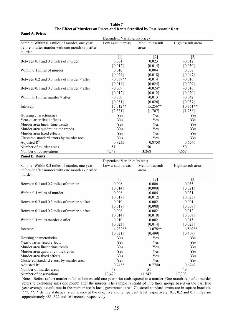
We report our results stratified by assault rate in Table 7 for prices in Panel A and

rental listings in Panel B. For brevity, we only report it for the within 0.3 mile sample

although we find qualitatively similar results using the entire sample and for the 0.2 mile

sample. For housing prices in Table 7 Panel A, we find that for the low assault rate areas (in

column 1) the coefficient for ‘Between 0.2 and 0.3 miles of murder × after’ is - 0.039 and

statistically significant while the coefficients are insignificant for the medium and high

assault areas in columns 2 and 3. This is consistent with low assault areas being more

impacted by a murder although we cannot prove causality of a murder affecting house prices

as our variables of interests, ‘Between 0.1 and 0.2 miles of murder × after’ and ‘Within 0.1

miles murder × after’ remain statistically insignificant with stratification. One exception is for

the medium assault areas where the coefficient for ‘Between 0.1 and 0.2 miles of murder ×

after’ is -0.024 and statistically significant. We find no effect of murders on rents when

19 LGA yearly population statistics are obtained from the Australian Bureau of Statistics (ABS) website ‘3218.0 - Regional Population Growth, Australia’.

23

stratifying by assault rate as shown in Table 7 Panel B. Overall, we do not find a pattern

between the effect of a murder on house prices or rents and the assault rate.

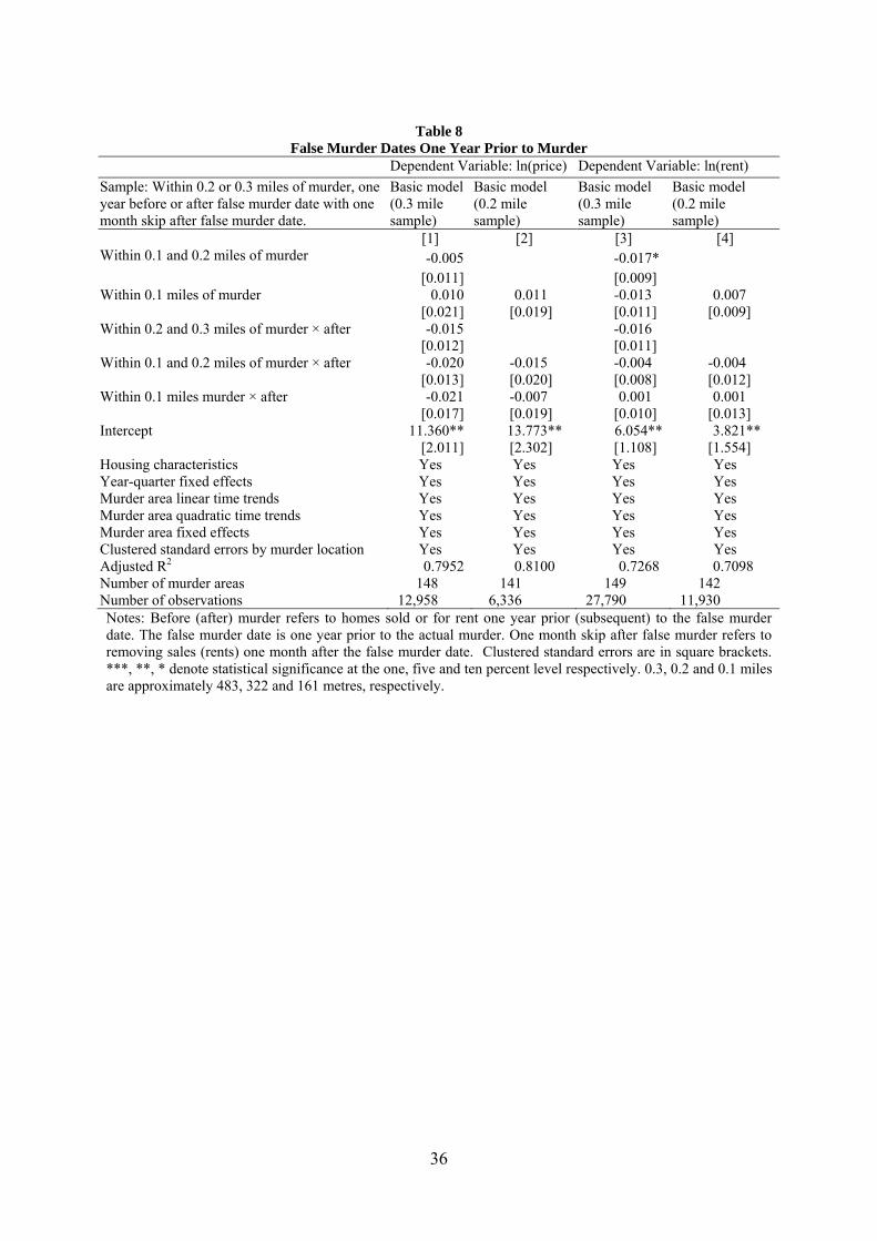
6.5.2 Falsification Tests using One Year Prior Murder Dates

Following Linden and Rockoff (2008) we test whether our findings that housing

prices falling within 0.3 miles of and after a murder may be driven by trends in prices prior to

the murder. As such we repeat our analysis except for using false murder dates that are one

year prior to the actual murder. We report our findings in Table 8. For housing prices in

columns 1 and 2 we find no statistically significant trends. This provides further support that

the price falls we find are due to the murders and not a negative price trend in the area. For

rental prices in columns 3 and 4 we also find no statistically significant trend.

6.5.3 The Effect of Nearby Murders on Housing Prices and Rents Two Years After

In this section we use an extended time frame of two years before and after the murder to

test whether the effect of a murder extends further than a year. We report our results in Table

9. We find no statistically significant falls in prices for the 0.3 sample (column 1) or rents

(columns 3 and 4) after the murder. However, for prices in the 0.2 sample in column 2 the

‘Within 0.1 miles murder × after’ coefficient is statistically significant with a value of 0.029.

This suggests that there is some evidence of the effect of a murder on prices extending

beyond one year.

7. Conclusion

Murder is the worst form of violent crime and has an enormous impact on people related

to the victims and on the neighbourhood in general. Our study attempts to measure the impact

of murders on house prices and rents of nearby homes by using the time and spatial

sparseness of murders in Sydney. We find evidence that the prices of homes within 0.2 miles

of a murder fall by about 3.9% one year after the murder. Homes slightly closer, within 0.1

24

miles, have similar falls. However, we find no evidence that murders with higher media

coverage have a greater impact on house prices compared to those with low media coverage.

Using false murder dates of one year prior, we find that the fall is not due to declining price

trends. However, the effect is short-lived as we find only some difference in housing prices

using a two-year window. We find no effect of murders on rents. Taken together, our findings

suggest that proximity to a murder affects nearby housing prices, particularly in the first year

after the incident; however greater media coverage of a murder does not worsen the fall in

property prices.

25

References

Congdon-Hohman, J. M. (2012). "The lasting effects of crime: The relationship of discovered methamphetamine laboratories and home values." Regional Science and Urban Economics.

Ditton, J. and J. Duffy (1983). "Bias in the newspaper reporting of crime news." British Journal of Criminology 23(2): 159-163.

Gibbons, S. (2004). "The Costs of Urban Property Crime." The Economic Journal 114(499): F441-F463.

Goldberger, A.S. (1968). "The interpretation and estimation of Cobb-Doulas Functions." Econometrica 35: 464-472.

Halvorsen, R. and Palmquist, R. (1980). "The interpretation of dummy variables in semilogarithmic equations." American Economic Review 70: 474-475.

Hellman, D. A. and J. L. Naroff (1979). "The impact of crime on urban residential property values." Urban Studies 16(1): 105-112.

Ihlanfeldt, K. and T. Mayock (2010). "Panel data estimates of the effects of different types of crime on housing prices." Regional Science and Urban Economics 40(2): 161-172.

Kennedy, P.E. (1981). "Estimation with correctly interpreted dummy variables in semilogarithmic equations." American Economic Review 71(4): 801.

Linden, L. and J. E. Rockoff (2008). "Estimates of the impact of crime risk on property values from Megan's Laws." American Economic Review 98(3): 1103-1127.

Lynch, A. K. and D. W. Rasmussen (2001). "Measuring the impact of crime on house prices." Applied Economics 33(15): 1981-1989.

Ozanne, L. and S. Malpezzi (1985). "The efficacy of hedonic estimation with the annual housing survey. Evidence from the demand experiment." Journal of Economic and Social Measurement 13(2): 153-172.

Petersen, M. A. (2009). "Estimating Standard Errors in Finance Panel Data Sets: Comparing Approaches." Review of Financial Studies 22(1): 435-480.

Pope, D. G. and J. C. Pope (2012). "Crime and property values: Evidence from the 1990's crime drop." Regional Science and Urban Economics 42: 177-188.

Pope, J. C. (2008). "Fear of crime and housing prices: Household reactions to sex offender registries." Journal of Urban Economics 64(3): 601-614.

Rizzo, M. J. (1979). "The cost of crime to victims: An empirical analysis." Journal of Legal Studies 8(1): 177-205.

Sharkey, P. (2010). "The acute effect of local homicides on children's cognitive performance." Proceedings of the National Academy of Sciences 107(26): 11733-11738.

Smith, S. J. (1984). "Crime in the News." British Journal of Criminology 24(3): 289-295. Thaler, R. (1978). "A note on the value of crime control: evidence from the property market."

Journal of Urban Economics 5(1): 137-145. Tita, G., T. Petras, et al. (2006). "Crime and Residential Choice: A Neighborhood Level

Analysis of the Impact of Crime on Housing Prices." Journal of Quantitative Criminology 22(4): 299-317.

van Garderen, K.J. and Shah, C. (2002). "Exact interpretation of dummy variables in semilogarithmic equations." Econometrics Journal 5: 149-159.

Wentland, S., B. Waller, et al. (2013). "Estimating the Effect of Crime Risk on Property Values and Time on Market: Evidence from Megan's Law in Virginia." Real Estate Economics, forthcoming.

26

White, H. (1980). "A heteroskedasticity-consistent covariance matrix estimator and a direct test for heteroskedasticity." Econometrica: Journal of the Econometric Society: 817-838.

Williams, P. and J. Dickinson (1993). "Fear of crime: read all about it? The relationship between newspaper crime reporting and fear of crime." British Journal of Criminology 33(1): 33-56.

27

Figure 1 Sydney Metropolitan Area and its 38 Local Government Areas

Source: http://en.wikipedia.org/wiki/File:Sydney_councils.png.

28

Figure 2 Murder Locations across Sydney 2005-2009

Notes: Triangles represent the location of each of the 160 murder incidents. Bold lines represent local government area borders while thin lines represent suburb borders. 1 mile is approximately 1,609 metres.

29

Table 1 Murder and Media Summary Statistics

Panel A. Murder Incident Count by Newspaper Articles One Month After Murder Murder incident count by articles in month after murder

Newspaper No articles 1 2 3 4 5 > 5 articles Total murders Daily Telegraph 26 51 29 24 14 8 8 160 Sydney Morning Herald 93 44 12 6 2 1 2 160 Both 24 40 25 21 17 13 20 160

Panel B. Murder Victim Cause of Death Cause of death Count Count (%) Mean articles Median articles

Stabbed 68 42.50 2.22 1.5

Shot 35 21.88 3.69 3

Bashed 15 9.38 3.20 3

Asphyxiation 14 8.75 3.57 3

Blunt Force 13 8.13 2.77 2

Fall 6 3.75 2.67 2

Unknown 4 2.50 1.00 1

Burnt 3 1.88 2.33 3

Poisoned 1 0.63 5.00 5

Vehicular 1 0.63 4.00 4

Total 160 100.00 2.81 2 Panel C. Location of Murder Incidents Location Count Count (%) Mean articles Median articles

House (single-family detached home) 53 33.13 2.85 2

Sidewalk/Street 34 21.25 2.03 1.5

Apartment /Unit 33 20.63 4.03 4

Other Commercial Venue 8 5.00 2.13 1

Nature Reserve/Park 7 4.38 2.29 3

Bar/Pub 5 3.13 3.00 3

Cafe/Restaurant 5 3.13 1.60 2

Other Housing Type 5 3.13 2.60 3

Car Park 3 1.88 1.33 2

Petrol Station 3 1.88 3.67 4

Shopping Mall 2 1.25 5.00 5

Hotel 1 0.63 1.00 1

Other (e.g. river, vacant land) 1 0.63 2.00 2

Total Incidents 160 100.00 2.81 2

30

Table 2 Mean Characteristics of Homes Sold and Rented in Sydney

Panel A. Sales Sales not within 0.3 miles

of murder area and one year before or after

Sales within 0.3 miles of a murder and one year before or after

Difference Standard Error

Sales price ($100,000) 7.335 6.091 -1.244** [0.060] % houses 0.564 0.327 -0.237** [0.004] Size of houses (1,000 square feet) 8.918 5.193 -3.725** [0.408] Number of bedrooms 2.84 2.291 -0.549** [0.009] Number of bathrooms 1.565 1.355 -0.210** [0.006] % with multiple parking 0.319 0.162 -0.157** [0.004] Number of observations 312,013 13,218 Panel B. Rents Rents not within 0.3 miles

of murder area and one year before or after

Rents within 0.3 miles of a murder and one year before or after

Difference Standard Error

Rental price ($100) 5.788 5.728 -0.060 [0.444] % houses 0.384 0.228 -0.156*** [0.003] Size of houses (1,000 square feet) 9.576 5.515 -4.061*** [0.388] Number of bedrooms 2.382 1.989 -0.393*** [0.006] Number of bathrooms 1.352 1.242 -0.110*** [0.004] % with multiple parking 0.193 0.094 -0.099*** [0.003] Number of observations 452,032 25,185 Notes: Before (after) murder refers to homes sold one year prior (subsequent) to a murder. Standard errors are in square brackets. ***, **, * denote statistical significance at the one, five and ten percent level respectively. 0.3 miles are approximately 483 metres.

31

Table 3 Sales and Rents One Year Before or After Different Numbers of Murder Incidents

Sample Sales Rents Within 0.3 miles of at least one murder incident 14,461 28,170 " " " of one murder incident 13,218 25,196 " " " of two murder incidents 964 2,380 " " " of three murder incidents 269 552 " " " of four murder incidents 10 41 " " " of five or more murder incidents 0 1 Notes: 0.3 miles is approximately 483 metres.

32

Table 4 Spatial Specification Check of Sales and Rents in Murder Locations

Panel A. Sales Sample: One year before murder and within 0.3 miles of murder

Log price % houses Size of houses (1,000 square feet)

Number of bedrooms

Number of bathrooms

% with multiple parking

[1] [2] [3] [4] [5] [6] Between 0.1 and 0.2 miles of murder -0.052 ** -0.054 ** -0.589 ** -0.123 *** -0.054 ** -0.023 ** [0.024] [0.024 [0.235 [0.047] [0.023] [0.011]

Within 0.1 miles of murder -0.067 -0.098 *** -0.742 *** -0.174 *** -0.066 ** -0.038 ** [0.040] [0.043] [0.276] [0.066] [0.032] [0.018]

Intercept 13.166 *** 0.243 *** 1.983 *** 2.183 *** 1.317 *** 0.124 *** [0.093] [0.069] [0.741] [0.191] [0.038] [0.027]

Year fixed effects Yes Yes Yes Yes Yes Yes Adjusted R2 0.012 0.026 0.003 0.019 0.006 0.015Number of observations 6,011 6,011 6,011 6,011 6,011 6,011Sample: One year before murder and within 0.2 miles of murder


Number of bedrooms

Number of bathrooms


[7] [8] [9] [10] [11] [12] Within 0.1 miles of murder -0.012 -0.042 -0.153 -0.052 -0.012 -0.015 [0.038] [0.027] [0.148] [0.059] [0.032] [0.017]

Intercept 13.126 *** 0.214 *** 1.148 *** 2.086 *** 1.279 *** 0.121 *** [0.097] [0.066] [0.380] [0.187] [0.046] [0.012]

Year fixed effects Yes Yes Yes Yes Yes YesAdjusted R2 0.015 0.023 0.011 0.012 0.002 0.012 Number of observations 2,967 2,967 2,967 2,967 2,967 2,967 Panel B. Rents Sample: One year before murder and within 0.3 miles of murder


Number of bedrooms

Number of bathrooms


[1] [2] [3] [4] [5] [6] Between 0.1 and 0.2 miles of murder -0.017 -0.02 -0.13 -0.072 * -0.047 *** -0.007 [0.022] [0.021] [0.103] [0.042] [0.016] [0.008]

Within 0.1 miles of murder -0.038 -0.061 * -0.083 -0.026 -0.032 0.022 [0.026] [0.033] [0.199] [0.072] [0.032] [0.025]

Intercept 6.224 *** 0.171 *** 0.902 *** 1.936 *** 1.254 *** 0.097 *** [0.042] [0.045] [0.250] [0.116] [0.023] [0.013]

Year fixed effects Yes Yes Yes Yes Yes Yes Adjusted R2 0.054 0.018 0.003 0.006 0.003 0.001 Number of observations 11,574 11,574 11,574 11,574 11,574 11,574 Sample: One year before murder and within 0.2 miles of murder


Number of bedrooms

Number of bathrooms


[7] [8] [9] [10] [11] [12] Within 0.1 miles of murder -0.022 -0.043 0.041 0.043 0.014 0.029 [0.025] [0.026] [0.181] [0.065] [0.031] [0.024]

Intercept 6.211 *** 0.159 *** 0.766 *** 1.86 *** 1.223 *** 0.084 *** [0.044] [0.054] [0.277] [0.140] [0.030] [0.019]

Year fixed effects Yes Yes Yes Yes Yes Yes Adjusted R2 0.061 0.017 0.002 0.029 0.003 0.002 Number of observations 5,753 5,753 5,753 5,753 5,753 5,753Notes: Clustered standard errors by murder area are in square brackets. ***, **, * denote statistical significance at the one, five and ten percent level respectively. 0.3, 0.2 and 0.1 miles are approximately 483, 322 and 161 metres, respectively.

33

Table 5 The Effect of Murders on Prices and Rents

Dependent Variable: ln(price) Dependent Variable: ln(rent)

Sample: One year before or after murder, with one month skip after murder. Either full, within 0.3 or within 0.2 mile of murder sample.

Basic model (full sample)

Basic model (0.3 mile sample)


Basic model distance (0.2 mile sample)

Basic model (full sample)



Basic model distance (0.2 mile sample)

[1] [2] [3] [4] [5] [6] [7] [8] Between 0.2 and 0.3 miles of murder -0.012 0.004 [0.009] [0.007]

Between 0.1 and 0.2 miles of murder -0.017 0.003 -0.016* -0.010 [0.015] [0.011] [0.009] [0.008]

Within 0.1 miles of murder -0.015 0.016 0.014 0.015 0.002 0.008 0.017 0.017 [0.019] [0.020] [0.017] [0.017] [0.016] [0.014] [0.012] [0.012]

Between 0.2 and 0.3 miles of murder × after 0.006 -0.016 -0.007 -0.002 [0.008] [0.013] [0.005] [0.013]

Between 0.1 and 0.2 miles of murder × after -0.008 -0.033** -0.037** -0.037** 0.004 -0.003 -0.016 -0.016 [0.009] [0.014] [0.016] [0.016] [0.006] [0.011] [0.016] [0.016]

Within 0.1 miles murder × after -0.021 -0.032* -0.042** -0.012 0.004 0.001 -0.012 -0.021 [0.018] [0.018] [0.019] [0.032] [0.012] [0.017] [0.020] [0.036]

Dist≤ 0.1 miles × after (0.1 miles = 1) -0.043 0.013 [0.039] [0.041]

Intercept 13.279** 14.957** 11.732** 11.810** 5.784** 7.027** 6.064** 6.066** [0.192] [1.077] [1.968] [1.982] [0.047] [1.001] [1.822] [1.825]

Housing characteristics Yes Yes Yes Yes Yes Yes Yes Yes Year-quarter fixed effects Yes Yes Yes Yes Yes Yes Yes Yes Suburb/murder area linear time trends Suburb Murder Murder Murder Suburb Murder Murder Murder Murder area quadratic time trends No Yes Yes Yes No Yes Yes Yes Suburb/murder area fixed effects Suburb Murder Murder Murder Suburb Murder Murder Murder Clustered standard errors by suburb/murder area Suburb Murder Murder Murder Suburb Murder Murder Murder Adjusted R2 0.8075 0.7732 0.8092 0.8092 0.7405 0.6997 0.6672 0.6672 Number of murder areas 151 151 142 142 151 151 146 146 Number of observations 243,430 12,678 6,172 6,172 350,811 27,001 11,988 11,988 Notes: Before (after) murder refers to homes sold one year prior (subsequent) to a murder. One month skip after murder refers to excluding sales one month after the murder. Clustered standard errors are in square brackets. ***, **, * denote statistical significance at the one, five and ten percent level respectively. 0.3, 0.2 and 0.1 miles are approximately 483, 322 and 161 metres, respectively.

34

Table 6 The Effect of Murders with High Media Coverage on Prices and Rents

Dependent Variable: ln(price) Dependent Variable: ln(rent) Sample: One year before or after murder, with one month skip after murder. Either full, within 0.3 or within 0.2 mile of murder sample.

Media interaction (full sample)

Media interaction (0.3 mile sample)


Media interaction (full sample)



[1] [2] [3] [4] [5] [6] Between 0.2 and 0.3 miles of murder

-0.006 0.012

[0.014] [0.011] Between 0.1 and 0.2 miles of murder

-0.004 0.000 -0.014 -0.023**

[0.024] [0.020] [0.014] [0.010] Within 0.1 miles of murder -0.003 0.001 0.004 0.029 0.010 0.032 [0.02] [0.020] [0.021] [0.026] [0.025] [0.022]

Between 0.2 and 0.3 miles of murder × after

-0.007 -0.034** -0.011 -0.010

[0.011] [0.013] [0.007] [0.024] Between 0.1 and 0.2 miles of murder × after

-0.029* -0.025 -0.043** -0.01 -0.015 -0.037

[0.015] [0.016] [0.018] [0.011] [0.018] [0.029] Within 0.1 miles murder × after -0.028 -0.056** -0.048** -0.003 -0.012 -0.039 [0.022] [0.021] [0.024] [0.023] [0.033] [0.039]

Between 0.2 and 0.3 miles of high media murder

-0.011 -0.015

[0.018] [0.015] Between 0.1 and 0.2 miles of high media murder

-0.024 0.005 0.213 -0.004 0.024 0.551

[0.026] [0.023] [2.489] [0.019] [0.016] [1.972] Within 0.1 miles of high media murder

-0.025 0.027 0.233 -0.053* -0.004 0.522

[0.037] [0.034] [2.48] [0.030] [0.029] [1.975] Between 0.2 and 0.3 miles of high media murder × after

0.026 0.036 0.007 0.021

[0.016] [0.025] [0.008] [0.026] Between 0.1 and 0.2 miles of high media murder × after

0.043* 0.016 0.011 0.029** 0.029 0.051

[0.026] [0.020] [0.027] [0.014] [0.019] [0.042] Within 0.1 miles of high media murder × after

0.012 0.048 0.012 0.013 0.029 0.039

[0.034] [0.036] [0.036] [0.025] [0.036] [0.029] Intercept 13.28** 14.786** 11.492** 5.784** 6.921** 5.547** [0.191] [1.084] [0.983] [0.047] [1.052] [0.15]

Housing characteristics Yes Yes Yes Yes Yes Yes Year-quarter fixed effects Yes Yes Yes Yes Yes Yes Suburb/murder area linear time trends

Suburb Murder Murder Suburb Murder Murder

Murder area quadratic time trends No Yes Yes No Yes Yes Suburb/murder area fixed effects Suburb Murder Murder Suburb Murder Murder Clustered standard errors by suburb/murder area

Suburb Murder Murder Suburb Murder Murder

Adjusted R2 0.8075 0.7733 0.8092 0.7405 0.6999 0.6674 Number of murder areas 151 151 142 151 151 146 Number of observations 243,430 12,678 6,172 350,811 27001 11,988 Notes: Before (after) murder refers to homes sold one year prior (subsequent) to a murder. One month skip after murder refers to excluding sales one month after the murder. Clustered standard errors are in square brackets. ***, **, * denote statistical significance at the one, five and ten percent level respectively. 0.3, 0.2 and 0.1 miles are approximately 483, 322 and 161 metres, respectively.

35

Table 7 The Effect of Murders on Prices and Rents Stratified by Past Assault Rate

Panel A. Prices Dependent Variable: ln(price)

Sample: Within 0.3 miles of murder, one year before or after murder with one month skip after murder

Low assault areas Medium assault areas

High assault areas

[1] [2] [3] Between 0.1 and 0.2 miles of murder 0.001 0.023 -0.012 [0.012] [0.014] [0.030]

Within 0.1 miles of murder 0.010 0.004 0.008 [0.024] [0.018] [0.047]

Between 0.2 and 0.3 miles of murder × after -0.039** -0.014 -0.016 [0.014] [0.024] [0.029]

Between 0.1 and 0.2 miles of murder × after -0.009 -0.024* -0.016 [0.012] [0.012] [0.020]

Within 0.1 miles murder × after -0.050 -0.013 -0.042 [0.031] [0.026] [0.037]

Intercept 15.512** 15.256** 10.361** [2.331] [1.707] [1.758]

Housing characteristics Yes Yes Yes Year-quarter fixed effects Yes Yes Yes Murder area linear time trends Yes Yes Yes Murder area quadratic time trends Yes Yes Yes Murder area fixed effects Yes Yes Yes Clustered standard errors by murder area Yes Yes Yes Adjusted R2 0.8235 0.8758 0.6766 Number of murder areas 51 50 50 Number of observations 4,743 3,268 4,667 Panel B. Rents Dependent Variable: ln(rent)

Sample: Within 0.3 miles of murder, one year before or after murder with one month skip after murder

Low assault areas Medium assault areas

High assault areas

[1] [2] [3] Between 0.1 and 0.2 miles of murder -0.008 -0.006 -0.033 [0.014] [0.009] [0.021]

Within 0.1 miles of murder 0.008 -0.004 -0.031 [0.018] [0.012] [0.023]

Between 0.2 and 0.3 miles of murder × after -0.010 -0.002 -0.001 [0.018] [0.008] [0.009]

Between 0.1 and 0.2 miles of murder × after 0.006 -0.002 0.012 [0.014] [0.010] [0.007]

Within 0.1 miles murder × after -0.010 0.002 0.015 [0.023] [0.014] [0.023]

Intercept 4.932** 3.078** 6.569** [0.521] [0.499] [0.407]

Housing characteristics Yes Yes Yes Year-quarter fixed effects Yes Yes Yes Murder area linear time trends Yes Yes Yes Murder area quadratic time trends Yes Yes Yes Murder area fixed effects Yes Yes Yes Clustered standard errors by murder area Yes Yes Yes Adjusted R2 0.7433 0.7740 0.6749 Number of murder areas 48 51 49 Number of observations 13,479 11,247 17,393 Notes: Before (after) murder refers to homes sold one year prior (subsequent) to a murder. One month skip after murder refers to excluding sales one month after the murder. The sample is stratified into three groups based on the past five year average assault rate in the murder area's local government area. Clustered standard errors are in square brackets. ***, **, * denote statistical significance at the one, five and ten percent level respectively. 0.3, 0.2 and 0.1 miles are approximately 483, 322 and 161 metres, respectively.

36

Table 8

False Murder Dates One Year Prior to Murder Dependent Variable: ln(price) Dependent Variable: ln(rent)

Sample: Within 0.2 or 0.3 miles of murder, one year before or after false murder date with one month skip after false murder date.





[1] [2] [3] [4] Within 0.1 and 0.2 miles of murder -0.005 -0.017* [0.011] [0.009]

Within 0.1 miles of murder 0.010 0.011 -0.013 0.007 [0.021] [0.019] [0.011] [0.009]

Within 0.2 and 0.3 miles of murder × after -0.015 -0.016 [0.012] [0.011]

Within 0.1 and 0.2 miles of murder × after -0.020 -0.015 -0.004 -0.004 [0.013] [0.020] [0.008] [0.012]

Within 0.1 miles murder × after -0.021 -0.007 0.001 0.001 [0.017] [0.019] [0.010] [0.013]

Intercept 11.360** 13.773** 6.054** 3.821** [2.011] [2.302] [1.108] [1.554]

Housing characteristics Yes Yes Yes Yes Year-quarter fixed effects Yes Yes Yes Yes Murder area linear time trends Yes Yes Yes Yes Murder area quadratic time trends Yes Yes Yes Yes Murder area fixed effects Yes Yes Yes Yes Clustered standard errors by murder location Yes Yes Yes Yes Adjusted R2 0.7952 0.8100 0.7268 0.7098 Number of murder areas 148 141 149 142 Number of observations 12,958 6,336 27,790 11,930 Notes: Before (after) murder refers to homes sold or for rent one year prior (subsequent) to the false murder date. The false murder date is one year prior to the actual murder. One month skip after false murder refers to removing sales (rents) one month after the false murder date. Clustered standard errors are in square brackets. ***, **, * denote statistical significance at the one, five and ten percent level respectively. 0.3, 0.2 and 0.1 miles are approximately 483, 322 and 161 metres, respectively.

37

Table 9 Price and Rents using Two Years Before and After Murder

Dependent Variable: ln(price) Dependent Variable: ln(rent) Sample: Within 0.2 or 0.3 miles of murder, two years before or after murder with one month skip after murder





[1] [2] [3] [4] Within 0.1 and 0.2 miles of murder -0.007 -0.017* [0.012] [0.009]

Within 0.1 miles of murder 0.014 0.014 -0.013 0.010 [0.021] [0.022] [0.011] [0.008]

Within 0.2 and 0.3 miles of murder × after 0.005 -0.016 [0.012] [0.011]

Within 0.1 and 0.2 miles of murder × after -0.006 -0.018 -0.004 -0.006 [0.015] [0.015] [0.008] [0.011]

Within 0.1 miles of murder × after -0.021 -0.029* 0.001 -0.004 [0.015] [0.015] [0.010] [0.015]

Intercept 9.983** 13.668** 6.054** 4.685** [0.695] [1.282] [1.108] [0.494]

Housing characteristics Yes Yes Yes Yes Year-quarter fixed effects Yes Yes Yes Yes Murder area linear time trends Yes Yes Yes Yes Murder area quadratic time trends Yes Yes Yes Yes Murder area fixed effects Yes Yes Yes Yes Clustered standard errors by murder area Yes Yes Yes Yes Adjusted R2 0.7700 0.8093 0.7268 0.7064 Number of murder areas 147 140 149 141 Number of observations 22,016 10,651 27,790 20,694 Notes: Before (after) murder refers to homes sold two years prior (subsequent) to a murder. One month skip after murder refers to excluding sales (rents) one month after the murder. Clustered standard errors are in square brackets. ***, **, * denote statistical significance at the one, five and ten percent level respectively. 0.3, 0.2 and 0.1 miles are approximately 483, 322 and 161 metres, respectively.

38

Appendix A Global Comparison of Yearly Intentional Homicides per 100,000

Year Sydney Australia Canada Japan United Kingdom

(England and Wales) USA

2003 1.62 1.52 1.54 0.50 1.71 5.57

2004 1.34 1.31 1.72 0.50 1.64 5.39

2005 1.14 1.27 1.84 0.46 1.44 5.53

2006 1.55 1.36 1.71 0.44 1.41 5.57

2007 1.19 1.22 1.64 0.40 1.45 5.48

2008 1.02 1.23 1.67 0.45 1.19 5.22

Average 1.31 1.32 1.69 0.46 1.48 5.46

39

Appendix B Murders Matched to BOCSAR Statistics

Year Murders reported in BOCSAR statistics

Murders matched to news media

% matched Number geocoded with accuracy

% geocoded

2003 60 50 83.33 42 70.00 2004 50 37 74.00 31 62.00 2005 43 37 86.05 30 69.77 2006 59 53 89.83 47 79.66 2007 46 36 78.26 30 65.22 2008 40 37 92.50 28 70.00 2009 50 45 90.00 40 80.00 2010 38 32 84.21 25 65.79 Total 386 327 84.72 273 70.73 Notes: Statistics count number of murder victims. 'With accuracy' refers to murder incidents where the exact location is found from court decisions, newspaper or police media releases or where a 0.1 miles radius covers the entire street where a murder incident is reported to have occurred.

40

Appendix C List of Housing Characteristic Variables

Variable Description Beds Number of beds Baths Number of bathrooms Multiple Parking 1 if home has two or more parking spots, 0 otherwise Area size Land area size of houses (square metres) Street type dummies 1 if a certain street type (e.g. avenue, highway, lane, street, road, etc.), 0 otherwise Housing type dummies 1 if a certain housing type (e.g. apartment, house, semi, studio, townhouse, villa,

etc.), 0 otherwise HasAirConditioning 1 if home has air conditioning, 0 otherwise HasAlarm 1 if home has alarm system, 0 otherwise HasBalcony 1 if home has balcony, 0 otherwise HasBarbeque 1 if home has barbeque, 0 otherwise HasBeenRenovated 1 if home has been renovated, 0 otherwise HasBilliardRoom 1 if home has billiard room, 0 otherwise HasCourtyard 1 if home has courtyard, 0 otherwise HasEnsuite 1 if home has ensuite, 0 otherwise HasFamilyRoom 1 if home has family room, 0 otherwise HasFireplace 1 if home has fire place, 0 otherwise HasGarage 1 if home has garage, 0 otherwise HasHeating 1 if home has heating, 0 otherwise HasInternalLaundry 1 if home has internal laundry, 0 otherwise HasLockUpGarage 1 if home has lock up garage, 0 otherwise HasPolishedTimberFloor 1 if home has polished timber floors, 0 otherwise HasPool 1 if home has swimming pool, 0 otherwise HasRumpusRoom 1 if home has rumpus room, 0 otherwise HasSauna 1 if home has sauna, 0 otherwise HasSeparateDining 1 if home has separate dining room, 0 otherwise HasSpa 1 if home has spa, 0 otherwise HasStudy 1 if home has study room, 0 otherwise HasSunroom 1 if home has sunroom, 0 otherwise HasTennisCourt 1 if home has tennis court, 0 otherwise HasWalkInWardrobe 1 if home has walk in wardrobe, 0 otherwise View dummies 1 if home has a certain view (e.g. bush, city, district, harbour, ocean, park, river, etc.),

0 otherwise

41

Appendix D Selection Criteria Statistics for Hedonic Price Models

Panel A. Full Sample Model Variables Adjusted R2 AIC BIC PRESS

1 Beds, baths, multiple parking, area size, street type dummies, housing type dummies

0.3790 -138,282 -379,161 50,141

2 Model 1 plus suburb fixed effects 0.8005 -411,210 -652,085 19,310

3 Model 2 plus year/quarter fixed effects and suburb linear time trends

0.8043 -415,136 -656,000 18,130

4 Model 3 plus all other housing characteristics

0.8074 -418,989 -659,852 17,662

Panel B. 0.3 Mile Sample Model Variables Adjusted R2 AIC BIC PRESS


0.3550 -8,169 -20,737 2,412

2 Model 1 plus murder area fixed effects 0.7613 -20,514 -33,076 902

3 Model 2 plus year/quarter fixed effects and murder area linear/quadratic time trends

0.7667 -20,630 -33,176 892


0.7731 -20,807 -33,326 961

Panel C. 0.2 Mile Sample Model Variables Adjusted R2 AIC BIC PRESS


0.3864 -4,538 -10,664 1,086

2 Model 1 plus murder area fixed effects 0.8013 -11,306 -17,422 354

3 Model 2 plus year/quarter fixed effects and murder area linear/quadratic time trends

0.8066 -11,316 -17,404 352


0.8090 -11,243 -17,281 660

42

Appendix E The Effect of Murders on Prices Extra Tests

Sample: Full sample Dependent Variable: ln(price) [1] [2] [3] [4]

Between 0.2 and 0.3 miles of murder 4.878** -0.059** 3.362** 0.288** [0.29] [0.02] [0.236] [0.022]

Between 0.1 and 0.2 miles of murder 4.864** -0.072** 3.351** 0.278** [0.289] [0.014] [0.233] [0.014]

Within 0.1 miles of murder 4.873** -0.066* 3.363** 0.289** [0.309] [0.036] [0.249] [0.032]

Between 0.2 and 0.3 miles of murder × after -0.004 -0.004 -0.015 -0.010 [0.018] [0.017] [0.014] [0.013]

Between 0.1 and 0.2 miles of murder × after -0.019 -0.022 -0.034** -0.030* [0.019] [0.018] [0.017] [0.016]

Within 0.1 miles murder × after -0.051** -0.053** -0.045** -0.041** [0.022] [0.021] [0.018] [0.017]

Intercept 14.457** 14.604** 13.403** 13.327** [0.071] [0.072] [0.041] [0.041]

Housing characteristics Yes Yes Yes Yes Year-quarter fixed effects Yes Yes Yes Yes Murder area linear time trends Yes Yes Yes Yes Murder area quadratic time trends Yes No Yes No Murder area fixed effects Yes Yes Yes Yes Suburb area fixed effects No No Yes Yes Clustered standard errors by murder area Yes Yes Yes Yes Adjusted R2 0.4534 0.4535 0.8069 0.8069 Number of murder areas 152 152 152 152 Number of observations 243,430 243,430 243,430 243,430 Notes: Before (after) murder refers to homes sold one year prior (subsequent) to a murder. One month skip after murder refers to excluding sales one month after the murder. Clustered standard errors are in square brackets. **, * denotes statistical significant at the five and ten percent level respectively. 0.3, 0.2 and 0.1 miles are approximately 483, 322 and 161 metres, respectively.

FINANCE DISCIPLINE GROUP fileprices fall by 3.9% for homes within 0.2 miles of the ... rental data...

Documents

Transcript of FINANCE DISCIPLINE GROUP fileprices fall by 3.9% for homes within 0.2 miles of the ... rental data...