
final+gur
61
i LOAD FLOW ANALYSIS OF RADIAL DISTRIBUTION NETWORK Thesis submitted in partial fulfillment of the requirements for the award of degree of Master of Engineering in Power Systems & Electric Drives By: Gurpreet Kaur (801041008) Under the supervision of: Dr. Smarajit Ghosh Head & Professor, EIED June 2012 ELECTRICAL & INSTRUMENTATION ENGG DEPARTMENT THAPAR UNIVERSITY PATIALA – 147004
description
Load flow
Transcript of final+gur

i
LOAD FLOW ANALYSIS OF RADIAL DISTRIBUTION NETWORK
Thesis submitted in partial fulfillment of the requirements for
the award of degree of
Master of Engineering in
Power Systems & Electric Drives
By:
Gurpreet Kaur
(801041008)
Under the supervision of:
Dr. Smarajit Ghosh
Head & Professor, EIED
June 2012
ELECTRICAL & INSTRUMENTATION ENGG
DEPARTMENT
THAPAR UNIVERSITY
PATIALA – 147004

ii

iii
ACKNOWLEDGMENT
First of all, I thank the Almighty God, who gave me the opportunity and strength to carry out this
work.
I would like to thank Dr. Smarajit Ghosh, Prof. & Head, EIED for the opportunity to work
with him, and also for his encouragement, trust and untiring support. Dr. Smarajit Ghosh has
been an advisor in the true sense both academically and morally throughout this thesis work.
Gratitude is accorded to Thapar University, Patiala, for providing all the necessary facilities to
complete my M.E. Thesis work.
The paucity of words does not compromise for extending my thanks to my all family members
whose uninterrupted love, inspiration and blessings helped me in completing this research report.
I am also thankful to the previous researchers whose published work has been consulted and
cited in my dissertation.
Gurpreet Kaur
801041008

iv
Dedicated to My Parents

v
ABSTRACT
In this thesis, a new method of load-flow technique for solving radial distribution networks by
sequential numbering scheme has been proposed. The aim of my thesis is to reduce data
preparation and propose a method to identify the nodes beyond each branch with less
computation. The simple transcendental equations have been used. Effectiveness of this load
flow method has been tested by taking an example of 69 node radial distribution networks) with
constant power (CP), constant current (CI), constant impedance (CZ) and composite load (CC)
modeling.
The superiority of the proposed method has been compared with the other method [19] available
in literature.

vi
TABLE OF CONTENTS
CERTIFICATE ii
ACKNOWLEDGEMENT iii
ABSTRACT v
LIST OF FIGURES viii
LIST OF TABLES ix
LIST OF SYMBOLS xi
1. INTRODUCTION 1-20
1.1 POWER DISTRIBUTION SYSTEMS 1
1.1.1 Global design of distribution networks 1
1.2 DISTRIBUTION SYSTEMS 2
1.2.1 Requirements of distribution system 3
1.2.2 Classification of distribution system 4
1.3 DISTRIBUTION SYSTEM TYPES 4
1.3.1 Radial type 5
1.3.2 Ring main type 6
1.3.3 Interconnected type 7
1.4 LOAD FLOW ANALYSIS 8
1.4.1 Choice of variables 11
1.4.2 Bus classification 12
1.4.3 Summary of variables in load flow analysis 14
1.4.4 Basic load flow equations 15
1.5 LITERATURE SURVEY OF LOAD FLOW 16
1.6 SCOPE OF THE RESEARCH 20
1.7 OBJECTIVES OF THE THESIS WORK 20
1.8 ORGANIZATION OF THESIS WORK 20

vii
2. PROPOSED METHOD 21-39
2.1 PROPOSED METHOD 21
2.2 ASSUMPTION 21
2.3 METHODOLOGY 21
2.4 IDENTIFICATION OF NODES BEYOND ALL BRANCHES 26
2.5 LOAD MODELLING 28
2.6 EXAMPLE 29
2.7 CONCLUSION 39
3. CONCLUSIONS AND FUTURE SCOPE OF WORK 40
3.1 CONCLUSION 40
3.2 FUTURE SCOPE OF WORK 40
REFERENCES 41-44
APPENDIX 45-50
A- Line and load data of 69 node Radial Distribution Network 45-49
B- Biography 50
viii
LIST OF FIGURES
FIGURE : CAPTION PAGE NUMBER NUMBER
Fig 1.1 : Single line diagram of distribution system 2
Fig 1.2 : Radial system 5
Fig 1.3 : Ring main system 7
Fig 1.4 : Interconnected system 8
Fig 2.1 : Single Line Diagram of Radial Distribution Network 22
Fig 2.2 : Branch of figure 2.1 23
Fig 2.3 : 69 Node Radial Distribution Network 30

ix
LIST OF TABLES
TABLE NUMBER : CAPTION PAGE NUMBER
Table 1.1 : Variables in Load Flow Analysis 14
Table 2.1 : Branch number (jj), Sending end node (m1 = IS(jj))
Receiving end node (m2 = IR(jj)) of figure 2.1 22
Table 2.2 : Nodes beyond Each Branch of Figure 2.1 25
Table 2.3 : Total Real power load and Reactive Power Load of 69- Node
Radial Distribution Network for CP, CI ,CZ, Composite load
modeling substation voltage 1.0 p.u. 31
Table 2.4 : Voltage of each node in p.u. of each node of 69-Node
Radial Distribution Network for CP, CI, CZ and CC load
modeling 32
Table 2.5 : Real power losses (kW) of each branch of 69-Node
Radial Distribution Network for CP, CI, CZ and CC load
modeling 34
Table 2.6 : Reactive power losses (kVAr) of each branch of 69-Node
Radial Distribution Network for CP, CI, CZ, CC load
modeling 36
Table 2.7 : Total real and reactive power losses of 69-Node Radial
Distribution Network for CP, CI, CZ and CC load
modeling 38
Table 2.8 : Node corresponding to minimum voltage of 69-Node
Radial Distribution Network for CP, CI, CZ and CC load
modeling 38
Table 2.9 : Comparison of relative CPU time and memory requirement
of the proposed method and method [19]. 39

x
Table A.1 : Line Data of 69- Node Radial Distribution Network 45
Table A.2 : Load Data of 69-Node Radial Distribution Network 48

xi
LIST OF SYMBOLS
NB : Total no. of Nodes
LN1 : Total no. of Branches
jj : Branch no. i.e., jj = 1,2,3,………,LN1
m1 : IS(jj) be the Sending end Node of branch-jj
m2 : IR(jj) be the Receiving end Node of branch-jj
m2 : Set of the Receiving end nodes beyond the branch-jj.
N(jj) : Total number of nodes beyond branch-jj
IE(jj, i) : Receiving end node beyond branch-jj.
ISS(jj) : IS(jj) for all jj
IRR(jj) : IR(jj) for all jj
V(m1) : Voltage of Sending end Node of branch- jj
V(m2) : Voltage of Receiving end Node of branch -jj
R(jj) : Resistance of branch- jj
X(jj) : Reactance of branch -jj
Z(jj) : Impedance of branch- jj
I(jj) : Current through the Branch-jj
Ir(jj) : Real Component of I(jj)
Im(jj) : Imaginary Component of I(jj)
PL(m2) : Active Power Load at Node m2
QL(m2) : Reactive Power Load at Node m2
IL(m2) : Load Current at Node m2
LP(jj) : Real Power Loss of Branch- jj
LQ(jj) : Reactive Power Loss of Branch- jj
DVMAX : Maximum Voltage Difference
kVAr : Amount of reactive power
kW : kilo watts

1
CHAPTER 1
INTRODUCTION
A planned and effective distribution network is the key to cope up with the ever increasing
demand for domestic, industrial and commercial load. The load-flow study of radial distribution
network is of prime importance for effective planning of load transfer. The power distribution
system and Load flow will be briefed in this introduction.
1.1 Power Distribution Systems
A Distribution network has typical characteristics of its own. Distribution networks design will
be introduced though this article along with clearly defining the differences between country and
urban distribution networks.
1.1.1 Global Design of Distribution Networks
The electric utility system is classified into the following three subsystems:
1. Generation
2. Transmission
Sub-transmission
3. Distribution
Sub-transmission is basically a subset of transmission as the voltage levels and protection
practices are almost similar, however it is sometimes treated as a Fourth Division. The
distribution system is further classified into the following:
Distribution Substation
Distribution Primary
Distribution Secondary

2
The voltage is reduced at the distribution substation, it is distributed into smaller amounts
according to the customer requirements and is supplied to many customers thorough the same
distribution substation. Thereby making the total number of transmission lines involved in the
distribution system more than that in the transmission system. The distribution system is
considered as ‘unbalanced’ because of the fact that in a distribution system most of the
customers are connected to only one of the three phases available, thus making the power flow in
each line different, which makes it unbalanced. The load-flow studies related to distribution
network emphasize on this characteristic.
1.2 Distribution Systems
Distribution system is defined as the part of power system which distributes electric power for
local utilization.
Figure 1.1 Single line diagram of distribution system.
In other words, the electrical system between the substation fed by the transmission system and
the consumer’s meter is known as the distribution system. The basic elements of a distribution
system are feeders, distributors and the service mains. Figure 1.1 depicts the single line diagram
of a typical low tension distribution system.

3
(i) Feeders: A feeder is essentially a conductor, connecting the localized generating station (or
the sub-station) to the desired area where power has to be distributed. In order to keep the current
in the feeder same throughout, generally no tappings are taken from the feeder. The current
carrying capacity is the main point of focus during design of a feeder.
(ii) Distributor: A distributor is basically a conductor from which tappings are taken for supply
to the consumers. In Figure1.1, AB, BC, CD, and DA represent the distributors. Since tapping
are taken at various places along the length of the distributor, the current through it is not
constant. The voltage drop across the length of the distributor is the main point of focus during
its design, as the statutory limit of voltage variations is ±10% of rated value at the consumer’s
terminal.
(iii) Service mains: A service mains is generally a small cable which connects the distributor to
the consumer terminals.
1.2.1 Requirements of a Distribution System
It is mandatory to maintain the supply of electrical power within the requirements of many types
of consumers. Following are the necessary requirements of a good distribution system:
1) Availability of power demand: Power should be made available to the consumers in large
amount as per their requirement. This is very important requirement of a distribution system.
2) Reliability: As we can see that present day industry is now totally dependent on electrical
power for its operation. So, there is an urgent need of a reliable service. If by chance, there is a
power failure, it should be for the minimum possible time at every cost. Improvement in
reliability can be made upto a considerable extent by
a) Reliable automatic control system.
b) Providing additional reserve facilities.

4
3) Proper voltage: Furthermost requirement of a distribution system is that the voltage variations
at the consumer terminals should be as low as possible. The main cause of changes in voltage
variation is variation of load on distribution side which has to be reduced. Thus, a distribution
system is said to be only good, if it ensures that the voltage variations are within permissible
limits at consumer terminals.
4) Loading: The transmission line should never be over loaded and under loaded.
5) Efficiency: The efficiency of transmission lines should be maximum say about 90%.
1.2.2 Classification of Distribution System A distribution system may be classified on the basis of:-
i) Nature of current: According to nature of current, distribution system can be classified as
a) AC distribution system.
b) DC distribution system.
ii) Type of construction: According to type of construction, distribution system is classified as
a) Overhead system
b) Underground system
iii) Scheme of operation: According to scheme of operation, distribution system may be
classified as:
a) Radial system
b) Ring main system
c) Interconnected system
1.3 Distribution System Types
Here the distribution type has been discussed on the basis of scheme of operation. All
distribution of electrical energy is done by constant voltage system. In practice, the following
three types of distribution circuits are generally used in distribution system:

5
1.3.1 Radial System
A schematic example of a radial distribution system is shown in Figure 1.2. In this system,
primary feeders take power from the distribution substation to the load areas by way of sub
feeders and lateral-branch circuits. This is the most common system used because it is the
simplest and least expensive to build. It is widely used in sparsely populated areas. A radial
system has only one power source for a group of customers
Radial feeders are characterized by having only one path for the power to flow from the source
(distribution substation) to each customer. If the distributor is connected to the supply system on
one end only, that system is called radial distribution system. A typical radial distribution system
is as shown below.
Figure 1.2 Radial System

6
The radial system is employed when the power is generated at low voltage and the substation is
located at the center of the load.
The consumers at the end of distributor would be subjected to serious voltage fluctuations when
the load on distribution changes. The advantages of radial system are its simplicity, and low cost,
the amount of switching equipment required is small and protective relaying is simple. The
major disadvantage of radial system is its lack of security of supply.It is not the most reliable
system, however, because a fault or short circuit in a main feeder may result in a power outage to
all the users served by the system. Service on this type of system can be improved by installing
automatic circuit breakers that will reclose the service at predetermined intervals. If the fault
continues after a predetermined number of closures, the breaker will be locked out until the fault
is cleared and service is restored.
1.3.2 Ring main system
The loop (or ring) distribution system is one that starts at a distribution substation, runs through
or around an area serving one or more distribution transformers or load centres, and returns to
the same substation. The loop system shown in Fig 1.3 is more expensive to build than the radial
type, but it is more reliable and may be justified in areas where continuity of service is
required—at a medical centre, for example. In the loop system, circuit breakers sectionalize the
loop on both sides of each distribution transformer connected to the loop. A fault in the primary
loop is cleared by the breakers in the loop nearest the fault, and power is supplied the other way
around the loop without interruption to most of the connected loads. If a fault occurs in a
section adjacent to the distribution substation, the entire load can be fed from one direction over
one side of the loop until repairs are made.
The ring main system has the following advantages:
a) There are very less voltage fluctuations at consumer’s terminals.
b) The system is very reliable as each distributor is fed with two feeders. In case, of fault in any
section of feeder, the continuity of supply is maintained.

7
Figure 1.3 Ring Main System
1.3.3 Interconnected system
The network system shown in Fig 1.4 is the most flexible type of primary feeder system. It
provides the best service reliability to the distribution transformers or load centres, particularly
when the system is supplied from two or more distribution substations. Power can flow from any
substation to any distribution transformer or load centre in the network system. The network
system is more flexible about load growth than the radial or loop system. Service can
readily be extended to additional points of usage with relatively small amounts of new
construction. The network system, however, requires large quantities of equipment and is,
therefore, more expensive than the radial system. For this reason it is usually used only in
congested, high load density municipal or downtown areas. When the feeder ring is energized by
two or more than two generating stations or sub stations, it is called inter-connected system.

8
Figure1.4 Interconnected Systems
The ring main system has the following advantages:
a) It increases the service reliability.
b) Any area fed from one generating station during peak load hours can be fed from other
generating station. This helps in decreasing reserve power capacity and increases the efficiency
of the distribution system.
1.4 Load Flow Analysis
The operating state of an entire power system; i.e. network of generators, transmission lines, and
loads representing areas ranging from small municipality to several states; can be described with
load-flow analysis. If the amount of power generated and consumed at different locations is

9
known then load flow analysis can be used to determine the other quantities. One of the
important quantities is voltage at different locations throughout the transmission system, for
which the alternating current (AC) consists of both magnitude and a time element or phase angle.
After determining the voltage at different locations, the current flowing through the entire
transmission link can be obtained. In a nutshell, if an amount of power delivered and where it
comes from is given, power flow analysis can be used to determine how it flows into its
destination. It is a very arduous task to determine what is happening at one part of a system for
given working conditions of another part of the system, even though their working is related by
deterministic laws of Physics. This is mainly because of the peculiar characteristics of AC
current and the complexity and size of a real power system; i.e. the elaborate topology including
many nodes and links, and large number of generator and loads. It is difficult to establish
relationships between all variables and obtain a formula, even for a small network of small
number of AC power sources and loads.
In mathematics, analytical solution cannot be obtained for it and a numerical solution is only
possible thorough a process of successive iterations. The entire system needs to be simulated to
find out the voltage or current at any given point. Earlier simulations were done through
miniature DC models of power system in use. DC power units were used to represent generators,
resistors for loads and appropriately sized wires for transmission lines. Then by measurement the
voltages and currents could be found out empirically. As an example, to find out the increase in
current on line A due to Generator X taking over power production from Generator Y, adjust the
values on X and Y and read the ammeter on line A. The DC model gives an approximation for
most practical purposes but not the exact match of the behavior of the AC system. Nowadays, a
computer can be used to represent both the DC and AC system, eliminating the need to build
these models physically, that accounts for peculiarities of the AC. Such a simulation uses load-
flow analysis.
Load flow utilizes a mathematical algorithm that approximates a solution through successive
iteration. These are basically a process of trial and error starting with an assumed value of array
of numbers for the entire system, it ten compares with the relationship of the numbers to the laws
of physics and continuously adjusts the numbers until the entire array is consistent with both

10
physical law and the conditions stipulated by the user. Practically, it is a computer program
taking information about power system as input from the user, and provides the complete
working of the system as output. Different computational techniques are used and various types
of information are chosen as input and output for different programs. The straightforward load-
flow program simply calculates the variables pertaining to a single, existing system condition.
There are also more involved programs known as optimal power flow which analyze a multitude
of hypothetical situations or system conditions and rank them according to some desired criteria.
Planning, design and operation of distribution system for industrial facilities require load flow
study, which is used to evaluate the effects of additions or modifications to generators, motors, or
other electrical loads and various equipment configurations. Modern systems are complex and
power can flow through various paths or branches. The Kirchoff’s laws determine distribution of
electric power flow among these branches.
Typically the input data is divided into
Bus data
Branch data
Generator data
Transformer data
Load data
In order to document the system load configuration that the solution applies for , this data is
included with every load flow output file. The load flow study should have the following criteria
that the system evaluated must meet:
Voltage criteria
Power flows on cables and transformers must be within equipment ratings.
Generator reactive outputs must not be more than the limits defined by the generator
capability curves.
The load flow analysis designs a system that has a good voltage profile during normal operation
and that will continue to operate acceptably when one or more lines become inoperative due to

11
line damage, lightning strokes, failure of transformers, etc. Also, load flow helps to study the size
and placement of power factor correction capacitors and the setting of generator scheduled
voltages and transformer tap positions.
The load flow study plays an important role in determining the best operation of existing systems
and planning the future expansion of power systems. In the nutshell, the load flow study gives
the magnitude and phase angle of the voltage at each bus and the real and reactive power flowing
in each line.
1.4.1 Choice of Variables
Since the load flow analysis deals with the known real and reactive power flows at each bus,
with known voltage magnitudes, the remaining voltage magnitudes and all the voltage angles can
be calculated from this information. The descriptive variables of the circuit should be organized
into ‘known variables’ and ‘unknown variables’ and then establish their relationships in terms of
equations. Then with the given information the equations should be manipulated to yield the
desired numerical results for the ‘unknown variables’. AC circuits utilize the dimension of time,
unlike in DC, where everything is static (except for the instant at which a switch is thrown), thus
AC describes an ongoing oscillation or movement. Each of the two main variables, voltage and
current, in an AC circuit has two numerical components: a magnitude component and a time
component. By convention, the magnitudes of AC voltage and current are described in terms of
root-mean-squared (r.m.s.) values and their timing in terms of a phase angle, which represents
the shift of the wave with respect to a reference point chosen in time. Thus, in order to describe
voltage or current at any given node in an AC circuit, it is essential to specify two quantities: a
voltage/current magnitude and a voltage/current angle.
While considering the amount of power transferred at any point of an AC circuit, two quantities
are taken into account: real and a reactive component. Thus, to completely determine an AC
circuit, exactly two pieces of information per node in is required. Lesser quantity will not lead to
a solution and more than two quantities would be redundant. Because of the nonlinear nature of
the load flow problem, it is impossible to find unique solution as more than one answer is
mathematically consistent with the given configuration. Thus, a ‘true’ solution is identified

12
among the various mathematical solutions available based on physical plausibility and common
sense. Also, it is possible that there might be no solution, as the provided information might not
correspond to any physical situation. But two variables per node are needed to determine
everything that is happening in the system. Practically, current is unknown and current through
the various circuit branches is calculated at the end of load flow analysis. Voltage is known for
some buses only but the amount of power going in or out of the bus is known for all. Load flow
analysis takes into the account all the known real and reactive power flows at each bus, and the
voltage magnitudes that are explicitly known, and then calculates the remaining voltage
magnitudes and all the voltage angles. After this the current magnitudes and angles from the
voltages are calculated. Real and refractive power can be calculated from voltage and current as
power being the product of voltage and current, and the relative phase angle between voltage and
current gives the respective contributions of real and reactive power. Although it is
mathematically difficult but, voltage or current magnitude and angle can be calculated if real and
reactive power are given, as each value of real and reactive power would be consistent with
many different possible combinations of voltages and currents. Thus, to choose the correct
combination, each node is checked in relation to its neighboring nodes in the circuit and a set of
voltages and currents are determined that are consistent all the way around the system.
1.4.2 Bus classification
There are three types of bus in power system. Each bus in the system has four variables: voltage
magnitude, voltage angle, real power and reactive power. During the operation of the power
system, each bus has two known variables and two unknowns. And following are the bus types:
Slack or Swing Bus
This bus is considered as the reference bus. The swing/slack bus is distinguished from others by
the fact that real and reactive powers at this bus are not specified. Usually, there is only one bus
of this type in a given power system. It must be connected to a generator of high rating relative
to the other generators. During the operation, the voltage of this bus is always specified and
remains constant in magnitude and angle. In addition to the generation, this bus is also

13
responsible for supplying the losses to the system. Here the voltage and the phase angle are
specified. Typically it is denoted as V1∠δ1 = 1∠0. The slack bus is numbered 1, for
convenience. Net power flows cannot be fixed in advance at every generating bus because the
network power losses are not known until the study has been completed. The generators at the
swing bus supply the difference between the specified real power into the system at the other
buses and the total system output plus losses. The power flow computes the real power P1 and
reactive power Q1.
Generator or Voltage Controlled Bus /PV Bus
During the operation the voltage magnitude at this bus is kept as constant. This bus has always a
generator connected to it where the voltage is controlled using the excitation and the power is
controlled using the prime mover control. Here the known are real power and voltage and
unknowns are reactive power and phase angle. PV buses comprise about 10% of all the buses in
a power system.
Sometimes, this bus is connected to a VAR device where the voltage can be controlled by
varying the value of the injected VAR to the bus.
Load Bus /PQ Bus
At this type of bus, the net powers real and reactive are known. The unknowns are voltage and
phase angle. A pure load bus (no generating facility at the bus)is a PQ bus. PQ buses are the
most common, comprising almost 80% of all the buses in a given power system.
Let us now articulate which variables will actually be given for each bus as inputs to the analysis.
Now we must distinguish between different types of buses. The two main types are generator
buses and load buses, for each of which it is required to specify concerned information. At the
load bus, we assume that the power consumption is given that is real and reactive power, for
each load bus. Referred to the symbols P and Q for real and reactive power, load buses are
denoted by PQ buses in load flow analysis.

14
At the generator buses we could in principle also specify P and Q. Here it arises two problems.
However, the first has to do with balancing the power needs of the system, and the second with
the actual operational control of generators. Therefore, it turns out to be more convenient to
specify P for all but one generator, the slack bus, and to use the generator bus voltage, V, instead
of the reactive power Q as the second variable. Therefore generator buses are called PV buses.
1.4.3 Summary of variables in Load Flow analysis
To summarize, there are three types of buses in load flow analysis and these are PQ (load bus),
PV (generator bus), and θ V (slack bus). If we are given the two input variables per bus, and
knowing all the fixed values of the system (i.e., the impedances of all the transmission links, as
well as the AC frequency), we have all the information which is required to determine the
operating state of the system. This means that we can find values for all the variables that were
not originally specified for each bus: θ and V for all the PQ buses; θ and Q for the PV buses; and
P and Q for the slack bus. The known and unknown variables for each type of bus are shown in
Table 1.1.
Table-1.1: Variables in Load Flow Analysis
Type of bus Variables known Variables unknown
Generator Real power (P)
Voltage magnitude (V)
Reactive power (Q)
Voltage angle (θ)
Load or generator Real power (P)
Reactive power (Q)
Voltage angle (θ)
Voltage magnitude (V)
Slack Voltage angle (θ)
Voltage magnitude (V)
Real power (P)
Reactive power (Q)

15
1.4.4 Basic Load Flow equations
Assuming a system having n buses, the injected current to the bus (node) k can be expressed as:
∑
Where is the proper element in the bus admittance matrix YBus
and,
| |∠ | |∠
The complex power at bus k ( k = 1,2, ..,n) is given as:
∑
| | ∑ | |
| |
| | ∑ | |
| |
where, Pk
and Qk
are the active and reactive power injection at bus k respectively. Thus, at each
bus we have two equations and four variables ( P, Q, δ, V ). Note that Y's and θ's are known from
network data. Actually, at each bus we have to specify two variables and solve for the remaining
two unknowns. Thus, for an N bus system 2N equations are solved. These 2N equations are
nonlinear equations as they involve products of variables as well as sine and cosine functions.

16
1.5 Literature Survey of Load Flow
Load-flow analysis has always been the top most concern of electrical engineers. It is an
important area of activity as it is the final link between bulk power systems and consumers. A
few methods have been discussed in the literature for load-flow analysis of distribution system.
As the distribution network is radial in nature having high R/X ratio whereas the transmission
system is loop in nature having X/R ratio. Therefore, the variables used for load flow analysis of
distribution systems are different from that of transmission systems. The distribution networks
are known as ill-conditioned. The conventional Gauss Seidel (GS) and Newton Raphson (NR)
method does not converge for the distribution networks.
In the literature, there are a number of efficient and reliable load flow solution techniques, such
as; Gauss-Seidel, Newton-Raphson and Fast Decoupled Load Flow [1-7]. In 1967, Tinney and
Hart [1] developed the classical Newton based power flow solution method. Later work by Stott
and Alsac [2] made the fast decoupled Newton method. The algorithm made by [2] remains
unchanged for different applications. Even though this method worked well for transmission
systems, its convergence performance is poor for most distribution systems due to their high R/X
ratio which deteriorates the diagonal dominance of the Jacobian matrix. For this very reason,
various other types of methods have been presented. Those methods consist of back/forward
sweeps on a ladder system. The formulation and the algorithm of those methods were different
from the Newton’s power flow method, which made those methods hard to be extended to other
applications in which the Newton method seemed more appropriate.
Iwamoto and Tamura [8] proposed an algorithm that is based on the modification of
conventional Newton-Raphson method for the solution of ill-conditioned power systems. The
solution of load flow problem never diverges by this algorithm but this method was quite time
consuming and complex.
Tripathy et al. [9] presented a Newton like method for solving ill-conditioned power systems.
Their method showed voltage convergence but could not be efficiently used for optimal power-
flow calculations.

17
Kersting [10] developed a technique for solving the load-flow problem in radial distribution
networks which is based on ladder network theory in the iterative routine. The solution was very
complicated and had many assumptions for a typical distribution system. In other words the
method was not designed to efficiently solve for meshed networks. Also Stevens et al. [11]
demonstrated that the ladder based technique was very fast but did not guarantee convergence.
Shirmohammadi et al. [12] presented a new compensation-based power flow method for radial
distribution system and then it was extended for the solution of weakly meshed distribution
system. The technique used is multiport compensation technique with some basic formulations
of Kirchoff’s law. The technique involves two step procedure in which first branch currents are
computed that is backward sweep and then bus voltages are updated that is forward sweep. This
method undoubtedly was more efficient than the Newton-Raphson power flow technique when
used for solving radial and weakly meshed distribution networks but needed a rigorous data
preparation. In improved version [13] branch power flow was used instead of branch complex
currents for weakly meshed transmission and distribution networks by Luo.
Renato [14] presented method in which the voltage magnitude at the receiving end is related to
the voltage at sending end and branch power flow. But the problem arises was that only voltage
magnitudes are computed not bus phase angles which was later used by Das et al. in [15].
Goswami and Basu [16] presented a direct method for solving radial and meshed distribution
networks where any node in the network could not be the junction of more than three branches.
Their method had the advantages of a no convergence problem, a guaranteed accurate solution
for any distribution system, and the ease with which composite loads could be represented. The
disadvantages were difficulty in numbering the nodes and branches. They had used sequential
branch and node numbering scheme.
Das et al. [17] had proposed a load-flow technique for solving radial distribution networks by
calculating the total real and reactive power fed through any node using power convergence with
the help of coding at the lateral and sub lateral nodes for large system that increased complexity

18
of computation. This method worked only for sequential branch and node numbering scheme.
They had calculated voltage of each receiving end node using forward sweep. They had taken the
initial guess of zero initial power loss to solve radial distribution networks. It can solve the
simple algebraic recursive expression of voltage magnitude and all the data can be easily stored
in vector form, thus saving an enormous amount of computer memory.
Haque [18] presented a new and efficient method for solving both radial and meshed networks
with more than one feeding node. The method first converted the multiple-source mesh network
into an equivalent single-source radial type network by setting dummy nodes. Then the
traditional ladder network method could be applied for the equivalent radial system. Unlike other
method effect of shunt and load admittances are incorporated in this method because of which it
can be employed to solve special transmission networks. This method has excellent convergence
for radial network.
Ghosh and Das [19] had proposed a load−flow method for solving radial distribution networks
which is based on the technique with nodes beyond branches using voltage convergence. Flat
voltage start had been considered. They had also shown that the proof of convergence. The
incorporation of charging admittances reduces losses and improves voltage profile. The main
drawback of this method was that it stores nodes beyond each branch. Computationally, the
proposed method is very efficient.
Eminoglu and Hocaoglu [20] presented a simple and efficient method to solve the power flow
problem in radial distribution systems which took into account voltage dependency of static
loads, and line charging capacitance. The method was based on the forward and backward
voltage updating by using polynomial voltage equation for each branch and backward ladder
equation. The proposed power flow algorithm has a robust convergence ability when compared
with the improved version of the classical forward-backward ladder method, i.e., Ratio-Flow.
Bijwe et al. [21] had proposed fuzzy based method for weakly meshed balanced and unbalanced
distribution systems. The method can handle simultaneous presence of several uncertainties in

19
input variables such as network parameters, load model coefficients, load forecast, and bus
shunts.
Sivanagaraju et al. [22] proposed a distinctive load flow solution technique which is used for
the analysis of weakly meshed distribution systems. A branch-injection to branch-current matrix
is formed (BIBC) and this matrix is formed by applying Kirchhoff’s current law for the
distribution network. Using the same matrix that is BIBC a solution for weakly meshed
distribution network is proposed.
Ghosh and Sherpa [23] proposed a method for load-flow solution of radial distribution
networks with minimum data preparation. Here the node and branch numbering need not to be
sequential like other available methods. This method only needs sending node, receiving node
and branch numbers if those were sequential. The presented method used the simple equation to
compute the voltage magnitude and had the capability to handle composite load modelling. This
method used the set of nodes of feeder, lateral(s) and sub lateral(s) if not sequential.
Aravindhababu et al. [24] proposed a simple and efficient branch-to-node matrix-based power
flow method for radial distribution systems but this method was unsuitable for optimal power
flow for which the NR method seems to be more appropriate. In that method any presence of sub
laterals complicates the matrix formation.
Augugliaro et al. [25] had proposed a method for the analysis of radial or weakly meshed
distribution systems supplying voltage dependent loads. The solution process is iterative and at
every step loads are simulated by impedances. Therefore it is necessary to solve a network made
up only of impedances; for radial systems, all the voltages and currents are expressed as linear
functions of a single unknown current and for mesh system two unknown currents for each
independent mesh. Advantages of this method are: its possibility to take into account of any
dependency of the loads on the voltage, very reduced computational requirements and high
precision of results.

20
1.6 Scope of the Research
Literature survey shows that a number of methods had been proposed for load-flow solution of
radial distribution networks. In some cases authors had used the data as it is without reducing
data preparation and in some cases authors have tried to reduce the data preparation. Since the
distribution system is radial in nature having high R/X ratio, the load flow methods become
complicated. There is a scope to propose software to compute the nodes beyond each branch
with less computation as compared to Ghosh and Das [19].
1.7 Objectives of the Thesis Work
The objective of this thesis work is to propose a new algorithm to identify nodes beyond each
branch without any rigorous computation technique. Hence load flow method will be faster and
require less memory.
1.8 Organization of Thesis Work
Chapter 1 shows the introduction of distribution system, literature survey on loadflow,
objectives of the research, scope of the research and organization of the research.
Chapter 2 presents the proposed method for loadflow analysis of radial distribution networks.
The assumption, solution methodology, load modelling, algorithms, examples and results and
the conclusion.
Chapter 3 presents the summary of conclusion and the future scope of further research work.
References present the list of previous papers published by researchers in load flow surveyed by
the author and also the books in this area.
Appendix A shows the line data and load data of 69 node radial distribution network available
in [4].
Appendix-B Biography

21
CHAPTER 2
PROPOSED METHOD
2.1 Proposed method
The distribution system is radial in nature whereas transmission system is loop in nature. The
distribution system has high R/X ratio whereas transmission system has high X/R ratio.
Convergence of load flow is utmost important. The load-flow methods proposed for transmission
systems do not converge for distribution systems. Literature survey of load-flow for radial
distribution networks has already been presented in Article 1.5 of Chapter1.
The voltage of each node is computed using simple transcendental equations. Although the
present method is based on forward sweep and backward sweep, it computes load-flow of any
radial distribution networks very efficiently.
A 69node radial distribution network with constant power (CP), constant current (CC),constant
impedance (CZ),composite has been considered .
2.2 Assumption
It is assumed that the three phase distribution network is balanced and the charging capacitance
has been neglected. The network can be represented by its single line diagram.
2.3 Methodology
Fig. 2.1 shows the single line diagram of a radial distribution network. Table 2.1 shows the
branch number, sendingend node and receivingend node of Figure 2.1.

22
Table 2.1: Branch number (jj), Sending end node (m1 = IS(jj)), Receiving end node
(m2 = IR(jj)) of Figure 2.1
Branch Number
(jj)
Sending end
m1 = IS(jj)
Receiving end
m2 = IR (jj)
1 1 2
2 2 3
3 3 4
4 4 5
5 5 6
6 3 7
7 7 8
8 8 9
9 5 10
10 10 11
1 2 3 4 5
6
7
8
9
10 Bold Numbers
represent
branch numbers
1 3 2 4 6 5
7
8
9
11
10
Figure 2.1 Single Line Diagram of Radial Distribution Network
S/S

23
Figure 2.2 shows a branch of Figure 2.1. For branchjj, m1 is the sendingend node and m2 is
the receivingend node.
Current through the branchjj is expressed by
2m 2)m(V
2)mjQ(2)mP(I(jj)
θZ
δ(m2)V(m2)δ(m1)V(m1)
where m2 are set of the receivingend nodes beyond the branchjj.
i.e.,
m22m 2)m(V
2)mjQ(2)mP(
(m2)V
jQ(m2)P(m2)
θZ
δ(m2)V(m2)δ(m1)V(m1)
i.e., jb)(a(m2)V
jQ(m2)P(m2)
θZ
δ(m2)V(m2)δ(m1)V(m1)
where
jjk
mr
m22m
(k)]jI(k)[I2)m(V
2)mjQ(2)mP(jba
i.e., θZ (m2)jb)V(aθZjQ(m2)][P(m2)(m2)Vδ(m2)V(m2)δ(m1)V(m1)
i.e., 0θZjQ(m2)][P(m2)θZ (m2)jb)V(a)δ(δV(m2)V(m1)V(m2) 21
2
i.e., 0jf)(e (m2)jd)V(c)δ(δV(m2)V(m1)V(m2) 21
2 (2.1)
where X(jj)] j[R(jj)](k)I j(k)[IθZjb)(ajdcjjk
mr
m1 m2
jj
Figure 2.2 Branch of figure 2.1

24
jjk
m
jjk
r
jjk
m
jjk
r R(jj) (k)IX(jj) (k)I jX(jj) (k)IR(jj) (k)I (2.2)
and X(jj)] jjj)jQ(m2)][R([P(m2)jfe
]Q(m2)R(jj))[P(m2)X(jj j Q(m2)X(jj)P(m2)R(jj) (2.3)
Putting 1 2 0 , we have from Eq. (2.1),
0fV(m2))sin ccos d(j
eV(m2))sin dcos c(V(m1)2
V(m2)
22
22
(2.4)
Equating real and imaginary parts of Eq. (2.4), we have
0eV(m2))sin dcos c(V(m1)2
V(m2) 22
(2.5)
0fV(m2))sin ccos d( 22 (2.6)
The roots of Eq. (2.5) will be real if
04e)sin dcos c(V(m1)2
22 (2.7)
where
jjk
m
jjk
r X(jj) (k)IR(jj) (k)Ic (2.8)
and Q(m2)X(jj)P(m2)R(jj)e (2.9)
The load current of any receivingend node m2 = IR(jj) of branchjj is expressed by
(m2)*V
jQL(m2)PL(m2)IL(m2)
(2.10)
The real and reactive power losses of branchjj are expressed by
R(jj)2
I(jj)LP (2.11)

25
and X(jj)2
I(jj)LQ (2.12)
respectively.
The current through branchjj is the sum of all load currents of all nodes beyond branchjj i.e.,
I(jj) =
N(jj)
1i
i)IE(jj,IL (2.13)
where N(jj) is the total number of nodes beyond branch jj and IE(jj, i) is the receiving-end node
beyond branchjj. Table 2.2 shows the nodes beyond each branch of Figure 2.1.
Table 2.2 Nodes beyond Each Branch of Figure 2.1
Branch
Number (jj)
Nodes beyond Branchjj Total Number of Nodes
beyond Branchjj
1 2,3,4,5,6,7,8,9,10,11 10
2 3,4,5,6,7,8,9,10,11 9
3 4,5,6,10,11 5
4 5,6,10,11 4
5 6 1
6 7,8,9 3
7 8,9 2
8 9 1
9 10,11 2
10 11 1
26
To compute the current through each branch, the storing of nodes beyond each branch is required
which is a tedious task for any network having large number of nodes and laterals and
sublaterals. To reduce the computational work a method is proposed below. This method only
needs the starting node of each lateral and sublateral.
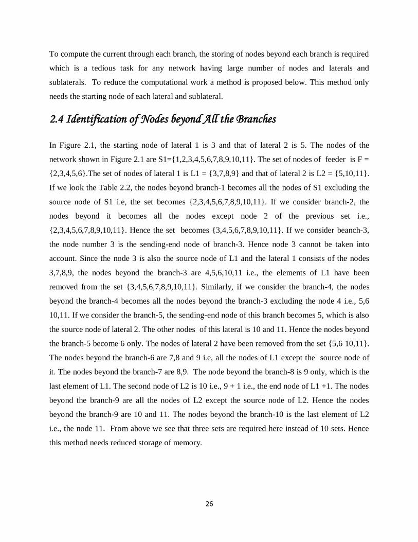
2.4 Identification of Nodes beyond All the Branches
In Figure 2.1, the starting node of lateral 1 is 3 and that of lateral 2 is 5. The nodes of the
network shown in Figure 2.1 are S1={1,2,3,4,5,6,7,8,9,10,11}. The set of nodes of feeder is F =
{2,3,4,5,6}.The set of nodes of lateral 1 is L1 = {3,7,8,9} and that of lateral 2 is L2 = {5,10,11}.
If we look the Table 2.2, the nodes beyond branch-1 becomes all the nodes of S1 excluding the
source node of S1 i.e, the set becomes {2,3,4,5,6,7,8,9,10,11}. If we consider branch-2, the
nodes beyond it becomes all the nodes except node 2 of the previous set i.e.,
{2,3,4,5,6,7,8,9,10,11}. Hence the set becomes {3,4,5,6,7,8,9,10,11}. If we consider beanch-3,
the node number 3 is the sending-end node of branch-3. Hence node 3 cannot be taken into
account. Since the node 3 is also the source node of L1 and the lateral 1 consists of the nodes
3,7,8,9, the nodes beyond the branch-3 are 4,5,6,10,11 i.e., the elements of L1 have been
removed from the set {3,4,5,6,7,8,9,10,11}. Similarly, if we consider the branch-4, the nodes
beyond the branch-4 becomes all the nodes beyond the branch-3 excluding the node 4 i.e., 5,6
10,11. If we consider the branch-5, the sending-end node of this branch becomes 5, which is also
the source node of lateral 2. The other nodes of this lateral is 10 and 11. Hence the nodes beyond
the branch-5 become 6 only. The nodes of lateral 2 have been removed from the set {5,6 10,11}.
The nodes beyond the branch-6 are 7,8 and 9 i.e, all the nodes of L1 except the source node of
it. The nodes beyond the branch-7 are 8,9. The node beyond the branch-8 is 9 only, which is the
last element of L1. The second node of L2 is 10 i.e., 9 + 1 i.e., the end node of L1 +1. The nodes
beyond the branch-9 are all the nodes of L2 except the source node of L2. Hence the nodes
beyond the branch-9 are 10 and 11. The nodes beyond the branch-10 is the last element of L2
i.e., the node 11. From above we see that three sets are required here instead of 10 sets. Hence
this method needs reduced storage of memory.

27
The algorithm of proposed software to identify the nodes beyond each branch is shown below.
Step 1 : Start
Step 2 : Read total number of branches (jj) and total number of nodes (NB).
Step 3 : Read the set of all nodes, set of nodes of laterals and sublaterals.
Step 4 : k = 1
Step 5 : Check the first element of the main set of nodes (M) and the first
element of laterals and sublaterals.
Step 6 : If it does not match, remove the first element of the of the main set
of nodes and get the subset (SB). Otherwise, remove the elements
of the set with which the first element of M matches and get the
subset (SB).
Step 7 : M is replaced by SB in the first iteration and in all other iteration
SB(old) is replaced by SB(new).
Step 8 : k = k +1
Step 9 : If k ≤ jj , go to Step 5 else go to Step-10.
Step 10 : Stop
The complete algorithm for computation of voltage of each node and losses of the network is
shown below.
The algorithm for computation the value of VSI at all nodes and identification of most sensitive
node is presented below.
Step 1 : Read the system data
Step 2 : Set V(i) =1.0 + j 0.0 for all i i.e., i =1,2,….,NB
Set VV(i) = V(i) for all i i.e., i = 1,2,…….,NB
Step 3 : Set ISS(jj) = IS(jj) and IRR(jj) = IR(jj) for
jj = 1,2,3,………,LN1
Step 4 : Set iteration count m =1
Step 5 : Set kMAX = 100(say)

28
Step 6 : Set DVMAX = 0.0 and = 0.00001
Step 7 : Identify the nodes beyond each branch using proposed method.
Step 8 : Compute load currents IL(m2) for all the node m2 i.e., for
m2 =2,3,4,….,NB using Eq. (2.10).
Step9 : Compute the current through each branch i.e., I(k) for all k i.e.,
k = 1,2,3,…..,jj using Eq. (2.13).
Step 10 : Set jj =1
Step 11 : Set m1 = ISS(jj) and m2 = IRR(jj). Compute receivingend voltage
V(m2) for all m2 using the feasible root of Eq. (2.5).
Step 12 : Compute the absolute change in voltage at node m2 i.e.,
DV(m2) = ABS(|V(m2)| |VV(m2)|)
Step 13 : jj = jj + 1
Step 14 : If jj < LN1, go to Step11, otherwise go to Step15
Step 15 : Find max value of DV(m2) from DV(m2) for m2 =2,3,4,….,NB.
Step 16 : DVMAX = DV(m2)
Step 17 : If DVMAX < go to Step21 else go to Step8.
Step 18 : m = m + 1
Step 19 : Set VV(m2) = V(m2) for m2 = 2,3,……….,NB.
Step 20 : If m < kMAX, go to Step8, otherwise go to Step22.
Step 21 : Print “Solution has converged”. Display the result.
Step22 : Print “Does not converge”.
2.5 Load Modeling
Load modeling has a crucial role in voltage stability analysis of a distribution network system.
Every load depends upon the voltage and frequency in the distribution system. A balanced load
is being considered in this thesis that can be represented either as constant power, constant
current, constant impedance or as an exponential load. The method of load-flow analysis must
have the capability to handle all types of load modeling. Equation (2.14) and (2.15) shows the
load modeling.

29
( ) ( )
(2.14)
( ) [ ( ) ( )
( )] (2.15)
where, and are nominal real and reactive power respectively and V(FN(i,j)) is the voltage at
node m2.
For all the loads, Eq. (2.14) and Eq. (2.15) are modeled as
(2.16)
(2.17)
For constant power (CP) load = = 1 and = = 0 for i = 1, 2, 3. For constantcurrent (CI)
load = = 1 and = = 0 for i = 0, 2, 3. For constant impedance (CZ) load = = 1 and
= = 0 for i = 0, 1, 3. Composite load modeling is combination of CP, CI and CZ. For
composite load = = 0 and = = 1 for i = 0, 1, 2. For exponential load = = 1 and
= = 0 for i = 0, 1, 2 and e1 and e2 are 1.38 and 3.22 respectively.
2.6 Example
One example has been considered to demonstrate the effectiveness of the proposed method. The
example is 69-node radial distribution network (nodes have been renumbered with Substation as
node 1) shown in Figure 2.3. Data for this system is available in [4] shown in Appendix-A. Table
2.3 shows the total load on the system for constant power (CP), constant current (CI), constant
impedance (CZ) and composite load modeling (CC) respectively. Table 2.4 shows the voltage of
each node in p.u. for constant power (CP), constant current (CI), constant impedance (CZ) and
composite load modeling (CC) respectively. Real power losses (kW) of each branch for this
system for CP, CI, CZ and Composite load (40% CP + 30% CI + 30% CZ) modeling is shown
in Table 2.5.
Reactive power losses (kVAr) of each branch for this system for CP, CI, CZ and Composite load
(40% CP + 30% CI + 30% CZ) modeling are shown in Table 2.6.
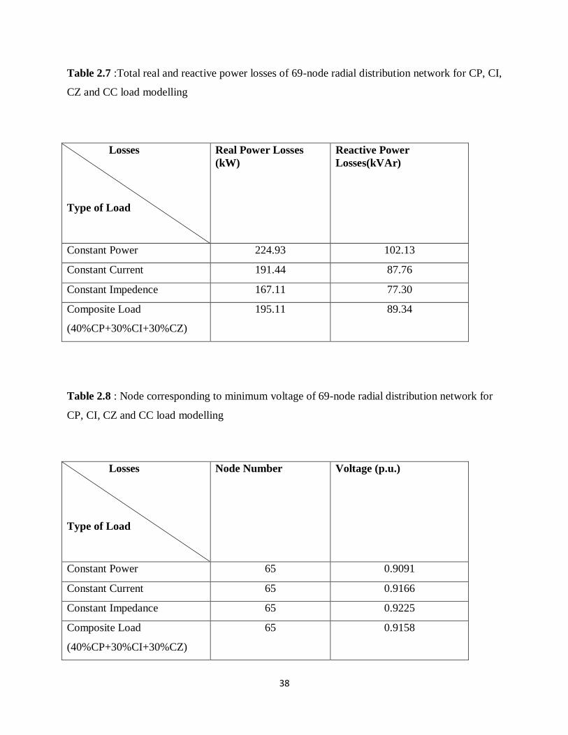
Table 2.7 shows the total losses of the system. Table 2.8 shows the node number of this system
having minimum voltage and its value in p.u. Table 2.9 shows the relative values of CPU time
and memory requirement. Base values for this system are12.66 kV and 100 MVA respectively.

30
S/
S
1 2
3
4 5 6 7 8 9 10 11 12 13 14 15 16 17
28
29
30
31
32
33
34
35
36 37 38 39 40 41 42 43 44 45 46
47
48
49
50
51
52
53
54
55
56
57
58
59
60
61
62
63
64
65
66
67
68
69
18
19
20
21
22
23
24
25
26
27
Figure 2.3 69 node radial distribution network

31
Table 2.3: Total Real power load and Reactive Power Load of 69node radial distribution
networks for CP, CI, CZ, Composite load modelling for substation voltage 1.0 pu
Type of load modelling
69node
radial distribution network
Real power load
(kW)
Reactive power load
(kVAr)
Constant Power 3801.89 2692.59
Constant Current 3633.45 2573.05
Constant Impedance 3495.96 2475.52
Composite load 3651.92 2586.17

32
Table 2.4 Voltage of each node in p.u. of each node of 69-node radial distribution network for
CP, CI, CZ and CC load modelling
Node
Number
Voltage (p.u.)
for CP load
Voltage (p.u.)
for CI load
Voltage (p.u.)
for CZ load
Voltage (p.u.)
for CC load
1
2
3
4
5
6
7
8
9
10
11
12
13
14
15
16
17
18
19
20
21
22
23
24
25
26
27
28
29
30
31
32
33
34
35
36
37
38
39
40
1.0000
0.9999
0.9999
0.9998
0.9990
0.9900
0.9807
0.9785
0.9774
0.9724
0.9713
0.9681
0.9652
0.9623
0.9595
0.9589
0.9580
0.9580
0.9576
0.9573
0.9568
0.9568
0.9567
0.9566
0.9564
0.9563
0.9563
0.9999
0.9998
0.9997
0.9997
0.9996
0.9993
0.9990
0.9989
0.9999
0.9997
0.9995
0.9995
0.9995
1.0000
0.9999
0.9999
0.9998
0.9990
0.9907
0.9820
0.9800
0.9789
0.9741
0.9730
0.9700
0.9672
0.9644
0.9617
0.9612
0.9603
0.9603
0.9599
0.9596
0.9591
0.9591
0.9591
0.9589
0.9587
0.9587
0.9587
0.9999
0.9998
0.9997
0.9997
0.9996
0.9993
0.9990
0.9989
0.9999
0.9997
0.9995
0.9995
0.9995
1.0000
0.9999
0.9999
0.9998
0.9991
0.9912
0.9831
0.9811
0.9801
0.9755
0.9744
0.9715
0.9688
0.9662
0.9635
0.9630
0.9622
0.9622
0.9618
0.9615
0.9611
0.9611
0.9610
0.9608
0.9607
0.9606
0.9606
0.9999
0.9998
0.9997
0.9997
0.9996
0.9993
0.9990
0.9989
0.9999
0.9997
0.9995
0.9995
0.9995
1.0000
0.9999
0.9999
0.9998
0.9990
0.9906
0.9819
0.9798
0.9788
0.9739
0.9729
0.9698
0.9670
0.9642
0.9614
0.9609
0.9601
0.9601
0.9596
0.9593
0.9589
0.9589
0.9588
0.9587
0.9585
0.9584
0.9584
0.9999
0.9998
0.9997
0.9997
0.9996
0.9993
0.9990
0.9989
0.9999
0.9997
0.9995
0.9995
0.9995

33
41
42
43
44
45
46
47
48
49
50
51
52
53
54
55
56
57
58
59
60
61
62
63
64
65
66
67
68
69
0.9988
0.9985
0.9985
0.9985
0.9984
0.9984
0.9997
0.9985
0.9947
0.9941
0.9785
0.9785
0.9746
0.9714
0.9669
0.9625
0.9401
0.9290
0.9247
0.9197
0.9123
0.9120
0.9116
0.9097
0.9091
0.9712
0.9712
0.9678
0.9678
0.9988
0.9985
0.9985
0.9985
0.9984
0.9984
0.9997
0.9985
0.9947
0.9942
0.9799
0.9799
0.9764
0.9734
0.9693
0.9653
0.9448
0.9347
0.9308
0.9262
0.9195
0.9192
0.9189
0.9171
0.9166
0.9730
0.9730
0.9697
0.9697
0.9988
0.9985
0.9985
0.9985
0.9984
0.9984
0.9998
0.9985
0.9947
0.9942
0.9811
0.9811
0.9778
0.9750
0.9712
0.9676
0.9486
0.9392
0.9356
0.9314
0.9252
0.9249
0.9246
0.9230
0.9225
0.9744
0.9744
0.9712
0.9712
0.9988
0.9985
0.9985
0.9985
0.9984
0.9984
0.9997
0.9985
0.9947
0.9941
0.9798
0.9798
0.9762
0.9732
0.9691
0.9650
0.9443
0.9341
0.9301
0.9255
0.9187
0.9184
0.9181
0.9163
0.9158
0.9728
0.9728
0.9695
0.9695

34
Table 2.5 : Real power losses (kW) of each branch of 69-node radial distribution network for
CP, CI, CZ and CC load modelling
Branch
Number
For CP load For CI load For CZ load For CC load
1
2
3
4
5
6
7
8
9
10
11
12
13
14
15
16
17
18
19
20
21
22
23
24
25
26
27
28
29
30
31
32
33
34
35
36
37
38
0.074951
0.074951
0.194856
1.936011
28.23028
29.33776
6.892022
3.373739
4.769865
1.013138
2.187400
1.282614
1.243801
1.204575
0.223837
0.320393
0.002604
0.104118
0.066933
0.107403
0.000536
0.005139
0.011185
0.006048
0.002495
0.000350
0.000347
0.002583
0.005829
0.001029
0.005143
0.012293
0.010403
0.000479
0.001405
0.015079
0.017323
0.005001
0.067705
0.067705
0.174678
1.683517
24.54849
25.50846
5.983242
2.915603
4.434904
0.941392
2.022315
1.176562
1.140558
1.104336
0.205210
0.293591
0.002385
0.095303
0.061266
0.098308
0.000490
0.004701
0.010233
0.005532
0.002282
0.000320
0.000347
0.002580
0.005818
0.001027
0.005134
0.012272
0.010382
0.000478
0.001403
0.015048
0.017282
0.004989
0.062190
0.062190
0.159379
1.495764
21.81073
22.66122
5.308249
2.576439
4.155425
0.881549
1.884989
1.088764
1.055105
1.021381
0.189795
0.271419
0.002204
0.088016
0.056582
0.090791
0.000453
0.004340
0.009446
0.005105
0.002106
0.000295
0.000346
0.002577
0.005808
0.001025
0.005125
0.012250
0.010362
0.000477
0.001400
0.015017
0.017242
0.004978
0.068501
0.068501
0.176892
1.711073
24.95031
25.92638
6.082432
2.965631
4.469410
0.948788
2.039418
1.187627
1.151333
1.114800
0.207155
0.296390
0.002408
0.096225
0.061859
0.099259
0.000495
0.004747
0.010333
0.005586
0.002304
0.000323
0.000347
0.002581
0.005819
0.001027
0.005135
0.012274
0.010384
0.000478
0.001403
0.015051
0.017287
0.004991

35
39
40
41
42
43
44
45
46
47
48
49
50
51
52
53
54
55
56
57
58
59
60
61
62
63
64
65
66
67
68
0.000199
0.048714
0.020117
0.002661
0.000514
0.006080
0.000013
0.023259
0.582158
1.631481
0.115753
0.001757
0.000044
5.781147
6.711319
9.124545
8.789956
49.68372
24.48876
9.505527
10.67081
14.02600
0.112051
0.134930
0.661155
0.041211
0.002624
0.000015
0.023324
0.000037
0.000198
0.048561
0.020053
0.002652
0.000512
0.006060
0.000013
0.023018
0.576136
1.613364
0.114405
0.001682
0.000042
4.833170
5.608976
7.611742
7.320890
41.38007
20.39595
7.916867
8.872423
11.66214
0.092768
0.111650
0.547084
0.034067
0.002476
0.000014
0.021849
0.000035
0.000197
0.048408
0.019990
0.002644
0.000510
0.006041
0.000012
0.022783
0.570257
1.595685
0.113090
0.001620
0.000040
4.153267
4.818533
6.528377
6.270060
35.44043
17.46834
6.780491
7.588098
9.973995
0.079058
0.095108
0.466027
0.028995
0.002351
0.000014
0.020611
0.000033
0.000198
0.048576
0.020059
0.002653
0.000512
0.006062
0.000013
0.023043
0.576742
1.615189
0.114541
0.001690
0.000042
4.937270
5.730026
7.777884
7.482258
42.29217
20.84552
8.091372
9.070159
11.92205
0.094894
0.114218
0.559669
0.034855
0.002490
0.000015
0.021999
0.000035

36
Table 2.6 :Reactive power losses (kVAr) of each branch of 69-node radial distribution network
for CP, CI, CZ, CC load modelling
Branch
Number
For CP load For CI load For CZ load For CC load
1
2
3
4
5
6
7
8
9
10
11
12
13
14
15
16
17
18
19
20
21
22
23
24
25
26
27
28
29
30
31
32
33
34
35
36
37
38
39
0.179883
0.179883
0.467655
2.267678
14.37738
14.94216
3.513286
1.717664
1.576560
0.335007
0.722881
0.423387
0.411026
0.398034
0.074005
0.105942
0.000886
0.034420
0.022025
0.035497
0.000176
0.001699
0.003698
0.001999
0.000825
0.000116
0.000851
0.006317
0.001927
0.000340
0.001700
0.004126
0.003439
0.000158
0.003450
0.036872
0.020235
0.005840
0.000232
0.162492
0.162492
0.419228
1.971928
12.50229
12.99185
3.050026
1.484414
1.465847
0.311283
0.668325
0.388380
0.376909
0.364911
0.067847
0.097080
0.000812
0.031506
0.020160
0.032491
0.000161
0.001554
0.003383
0.001828
0.000754
0.000106
0.000851
0.006310
0.001923
0.000339
0.001697
0.004119
0.003432
0.000158
0.003444
0.036797
0.020187
0.005826
0.000231
0.149256
0.149256
0.382510
1.752010
11.10798
11.54170
2.705940
1.311737
1.373472
0.291495
0.622942
0.359398
0.348670
0.337500
0.062750
0.089748
0.000750
0.029097
0.018619
0.030007
0.000149
0.001435
0.003123
0.001687
0.000696
0.000097
0.000850
0.006302
0.001920
0.000339
0.001694
0.004112
0.003425
0.000158
0.003437
0.036722
0.020140
0.005813
0.000230
0.164403
0.164403
0.424541
2.004205
12.70693
13.20469
3.100589
1.509885
1.477252
0.313728
0.673977
0.392032
0.380469
0.368369
0.068490
0.098005
0.000820
0.031810
0.020355
0.032805
0.000163
0.001569
0.003416
0.001846
0.000762
0.000107
0.000851
0.006310
0.001924
0.000339
0.001697
0.004120
0.003433
0.000158
0.003444
0.036804
0.020192
0.005828
0.000231

37
40
41
42
43
44
45
46
47
48
49
50
51
52
53
54
55
56
57
58
59
60
61
62
63
64
65
66
67
68
0.056915
0.023511
0.003102
0.000648
0.007665
0.000017
0.057463
1.424953
3.992005
0.283187
0.000896
0.000015
2.943734
3.418475
4.645748
4.477784
16.67685
8.218125
3.143511
3.239109
7.144279
0.057061
0.068674
0.336765
0.020990
0.000797
0.000005
0.007709
0.000013
0.056735
0.023436
0.003092
0.000646
0.007641
0.000017
0.056869
1.410212
3.947675
0.279889
0.000858
0.000014
2.461028
2.856986
3.875507
3.729411
13.88965
6.844629
2.618135
2.693209
5.940227
0.047241
0.056826
0.278663
0.017351
0.000752
0.000004
0.007222
0.000012
0.056557
0.023362
0.003082
0.000644
0.007617
0.000017
0.056289
1.395822
3.904418
0.276672
0.000826
0.000014
2.114825
2.454366
3.323914
3.194097
11.89595
5.862160
2.242332
2.303354
5.080350
0.040259
0.048406
0.237375
0.014768
0.000714
0.000004
0.006813
0.000011
0.056753
0.023444
0.003093
0.000646
0.007643
0.000017
0.056929
1.411697
3.952143
0.280222
0.000861
0.000014
2.514035
2.918644
3.960098
3.811615
14.19580
6.995499
2.675845
2.753232
6.072614
0.048324
0.058133
0.285073
0.017752
0.000756
0.000004
0.007271
0.000012
38
Table 2.7 :Total real and reactive power losses of 69-node radial distribution network for CP, CI,
CZ and CC load modelling
Losses
Type of Load
Real Power Losses
(kW)
Reactive Power
Losses(kVAr)
Constant Power 224.93 102.13
Constant Current 191.44 87.76
Constant Impedence 167.11 77.30
Composite Load
(40%CP+30%CI+30%CZ)
195.11 89.34
Table 2.8 : Node corresponding to minimum voltage of 69-node radial distribution network for
CP, CI, CZ and CC load modelling
Losses
Type of Load
Node Number Voltage (p.u.)
Constant Power 65 0.9091
Constant Current 65 0.9166
Constant Impedance 65 0.9225
Composite Load
(40%CP+30%CI+30%CZ)
65 0.9158

39
Table 2.9 : Comparison of relative CPU time and memory requirement of the proposed method
and method [19].
Relative Values→
Method
↓
Relative CPU time Relative memory
consumption
Proposed Method 1 1.49
Ghosh and Das [19] 1 2.18
2.7 Conclusion
In this thesis work an attempt has been made to propose a method, which can identify the nodes
beyond the branches in a simple way with less memory requirement. Using simple
transcendental equations, the expression for voltage without neglecting the voltage angle has also
been derived. The method has also been tested for constant power (CP), constant current (CI),
constant impedance (CZ) and composite (CC) load modelling. The superiority of the proposed
method with the existing method [19] has also been compared in terms of relative CPU time and
memory requirement.

40
CHAPTER 3
CONCLUSIONS & FUTURE SCOPE OF WORK
3.1 Conclusions
A method of loadflow analysis has been proposed for radial distribution networks based on the
new method to identify the nodes beyond each branch in a simple way. This has reduced the
computation. Effectiveness of the proposed method has been tested by one example 69 node
radial distribution networks with constant power load, constant current load, constant impedance
load and composite load. The voltage convergence has assured the satisfactory convergence in
all these cases. The superiority of the proposed method in terms of speed has been checked by
comparing with the other existing methods. The proposed method consumes less amount of
memory compared and less CPU time.
3.2 Future Scope of Work
The following are the scopes of future work
(i) Fuzzy loadflow analysis for unbalanced systems.
(ii) Loadflow analysis using Genetic Algorithms for unbalanced systems.

41
REFERENCES
[1] W.Tinney and C.Hart, “Power Flow Solution by Newton's Method”, IEEE Transactions on
Power Apparatus and Systems, Vol.PAS-86, no.11, pp.1449- 1460, November. 1967.
[2] B.Stott and O.Alsac, “Fast Decoupled Load-flow”, IEEE Transactions on Power Apparatus
and Systems, Vol.PAS-93, no.3, pp.859-869, May 1974.
[3] F. Zhang and C. S. Cheng, “A Modified Newton Method for Radial Distribution System
Power Flow Analysis”,IEEE Transactions on Power Systems, Vol.12, no.1,pp.389-397, February
1997.
[4] H. L. Nguyen, “Newton-Raphson Method in Complex Form”, IEEE Transactions on Power
Systems, Vol.12, no.3, pp.1355-1359, August 1997.
[5] Whei-Min Lin, Jen-HaoTeng, “Three-Phase Distribution Network Fast-Decoupled Power
Flow Solutions”, Electrical Power and Energy SystemsVol.22, pp.375-380, 2000.
[6] T. H. Chen, M. S. Chen, K. J. Hwang, P. Kotas, and E. A. Chebli, “Distribution System
Power Flow Analysis- A Rigid Approach”, IEEE Transactions on Power Delivery, Vol.6, no.3,
pp.1146-1153, July1991.
[7] J. H. Teng, “A Modified Gauss-Seidel Algorithm of Three-phase Power Flow Analysis In
Distribution Networks”, Electrical Power and Energy Systems Vol.24, pp.97-102, 2002.
[8] S.Iwamoto and Y.A.Tamura,“ Load-flow Calculation Method for Ill−Conditioned Power
Systems”, IEEE Transactions on Power Apparatus And Systems, Vol. PAS−100, no.4,
pp.1706−1713, April 1981.

42
[9] S.Tripathy,G.Prasad, O.Malik and G.Hope, “Load-Flow Solutions for Ill- Conditioned Power
Systems by a Newton-Like Method,” IEEE Transactions on Power Apparatus and Systems,
Vol.PAS-101, no.10, pp.3648-3657, 1982.
[10] W.H.Kersting, “A Method to Teach the Design and Operation of a Distribution System”,
IEEE Transactions on Power Apparatus and Systems; Vol.PAS-103, no.7, pp.1945-1952, 1984.
[11]R.A.Stevenset al., “Performance of Conventional Power Flow Routines for Real Time
Distribution Automation Application”, Proceedings 18th Southeastern Symposium on Systems
Theory: IEEE Computer Society: pp.196-200, 1986.
[12] D.Shirmohammadi, “A Compensation Based Power Flow Method for Weakly Meshed
Distribution and Transmission Network”, IEEE Transactions on Power Systems, Vol. 3, no. 2,
pp.753-762,1988.
[13] G. X. Luo, A. Semlyen, “Efficient Load Flow for Large Weakly Meshed Networks”,IEEE
Transactions on Power Systems, Vol.5, no.4, pp.1309-1316, 1990.
[14] C.G.Renato, “New Method for the Analysis of Distribution Networks”, IEEE Transactions
on Power Delivery; Vol.5, no.1, pp.391-396, January 1989.
[15] D. Das, D.P. Kothari, A Kalam, “Simple and Efficient Method for Load FlowSolution of
Radial Distribution Networks”, Electrical Power & Energy Systems, Vol.17, no.5, pp.335-346,
1995.
[16] S.Goswami and S.Basu, “Direct Solution of Distribution Systems”, IEE Proceedings on
Generation, Transmission and Distribution, Vol.138, no.1, pp.78- 88, January 1991.

43
[17] D.Das, H.S.Nagi and D.P.Kothari, “Novel Method for Solving Radial Distribution
Networks”, IEE Proceedings on Generation, Transmission and Distribution, Vol.141, no.4,
pp.291-298, July 1994.
[18] M.H.Haque, “Efficient Load-flow Method for Distribution Systems with Radial or Mesh
Configuration”, IEE Proceedings on Generation, Transmission, Distribution, Vol.143, no.1,
pp.33-39, January 1996.
[19] S.Ghosh and D.Das, “Method for Load−Flow Solution of Radial Distribution Networks”,
IEE Proceedings on Generation, Transmission and Distribution, Vol.146, no.6, pp.641–648,
November 1999.
[20] U.Eminoglu and M.H.Hocaoglu, “A New Power Flow Method For Radial Distribution
Systems Including Voltage Dependent Load Models”, Electric Power Systems Research Vol.76
pp.106–114, 2005.
[21] Bijwe PR, Vishwanadha Raju GK., “Fuzzy distribution power flow for weakly meshed
systems”, IEEE trans Power Syst. 2006;21(4):1645-52.
[22] S. Sivanagaraju, J. Viswanatha Raoand M. Giridhar,“A loop based loop flow method for
weakly meshed distribution network”, ARPN Journal of Engineering and Applied Sciences Vol.
3, no. 4, August 2008 ISSN 1819-6608.
[23] S. Ghosh and K.Sherpa, “An Efficient Method for Load−Flow Solution of Radial
Distribution Networks’’, Proceedings International Journal of Electrical Power and Energy
Systems Engineering, Spring 2008.
[24] A.Kumar and Aravindhababu, “An Improved Power Flow Technique for Distribution
Systems”, Journal of Computer Science, Informatics and Electrical Engineering Vol.3 Issue 1,
2009.

44
[25] Augugliaro A, Dusonchet L, Favuzza S, Ippolito MG, Riva Sanseverino E,“A Backward
sweep method for power flow solution in distribution networks”, Electrical Power and Energy
Systems 32 (2010) 271–280
[26] ME thesis by Apoorva Saxena ,“Load-flow analysis of Radial Distribution Networks with
Reduced Data Preparation”, from Thapar University under the supervision of Dr. Smarajit Ghosh
(Head & Professor, EIED) in June 2008.
[27] ME thesis by Amarinder Singh from Thapar University under the supervision of Dr.
Smarajit Ghosh (Head & Professor, EIED) in June 2008.

45
APPENDIX A
LINE & LOAD DATA OF 69 NODE RADIAL
DISTRIBUTION NETWORK
Table A.1 Line Data of 69 Node Radial Distribution Network
Branch
Number
Sendingend Receivingend Branch
Resistance ()
Branch
Reactance ()
1 1 2 0.0005 0.0012
2 2 3 0.0005 0.0012
3 3 4 0.0015 0.0036
4 4 5 0.0251 0.0294
5 5 6 0.3660 0.1864
6 6 7 0.3811 0.1941
7 7 8 0.0922 0.0470
8 8 9 0.0493 0.0257
9 9 10 0.8190 0.2707
10 10 11 0.1872 0.0619
11 11 12 0.7114 0.2351
12 12 13 1.0300 0.3400
13 13 14 1.0440 0.3450
14 14 15 1.0580 0.3496
15 15 16 0.1966 0.0650
16 16 17 0.3744 0.1238

46
17 17 18 0.0047 0.0016
18 18 19 0.3276 0.1083
19 19 20 0.2106 0.0696
20 20 21 0.3416 0.1129
21 21 22 0.0140 0.0046
22 22 23 0.1591 0.0526
23 23 24 0.3463 0.1145
24 24 25 0.7488 0.2475
25 25 26 0.3089 0.1021
26 26 27 0.1732 0.0572
27 3 28 0.0044 0.0108
28 28 29 0.0640 0.1565
29 29 30 0.3978 0.1315
30 30 31 0.0702 0.0232
31 31 32 0.3510 0.1160
32 32 33 0.8390 0.2816
33 33 34 1.7080 0.5646
34 34 35 1.4740 0.4873
35 3 36 0.0044 0.0108
36 36 37 0.0640 0.1565
37 37 38 0.1053 0.1230
38 38 39 0.0304 0.0355
39 39 40 0.0018 0.0021
40 40 41 0.7283 0.8509
41 41 42 0.3100 0.3623
42 42 43 0.0410 0.0478

47
43 43 44 0.0092 0.0116
44 44 45 0.1089 0.1373
45 45 46 0.0009 0..0012
46 4 47 0.0034 0.0084
47 47 48 0.0851 0.2083
48 48 49 0.2898 0.7091
49 49 50 0.0822 0.2011
50 8 51 0.0928 0.0473
51 51 52 0.3319 0.1114
52 9 53 0.1740 0.0886
56 53 54 0.2030 0.1034
53 54 55 0.2842 0.1447
54 55 56 0.2813 0.1433
55 56 57 1.5900 0.5337
56 57 58 0.7837 0.2630
57 58 59 0.3042 0.1006
58 59 60 0.3861 0.1172
59 60 61 0.5075 0.2585
60 61 62 0.0974 0.0496
61 62 63 0.1450 0.0738
62 63 64 0.7105 0.3619
63 64 65 1.0410 0.5302
64 11 66 0.2012 0.0611
65 66 67 0.0047 0.0014
67 12 68 0.7394 0.2444
68 68 69 0.0047 0.0016

48
Table A.2 Load Data of 69 Node Radial Distribution Network
Node
Number
PL(kW) QL(kVAr) Node
Number
PL(kW) QL(kVAr)
1 00.00 00.00 36 26.00 18.55
2 00.00 00.00 37 26.00 18.55
3 00.00 00.00 38 00.00 00.00
4 00.00 00.00 39 24.00 17.00
5 00.00 00.00 40 24.00 17.00
6 2.600 2.200 41 1.200 1.000
7 40.40 30.00 42 00.00 00.00
8 75.00 54.00 43 6.000 4.300
9 30.00 22.00 44 00.00 00.00
10 28.00 19.00 45 39.22 26.30
11 145.0 104.0 46 39.22 26.30
12 145.0 104.0 47 00.00 00.00
13 8.000 5.000 48 79.00 56.40
14 8.000 5.500 49 384.7 274.0
15 00.00 00.00 50 384.7 274.0
16 45.50 30.00 51 40.50 28.30
17 60.00 35.00 52 3.600 2.700
18 60.00 35.00 53 4.350 3.500
19 00.00 00.00 54 26.40 19.00
20 1.000 00.60 55 26.00 17.20
21 114.0 81.00 56 00.00 00.00

49
22 5.000 3.500 57 00.00 00.00
23 00.00 00.00 58 00.00 00.00
24 28.00 20.00 59 100.0 72.00
25 00.00 00.00 60 00.00 00.00
26 14.00 10.00 61 1244.0 888.0
27 14.00 10.00 62 32.00 23.00
28 26.00 18.60 63 00.00 00.00
29 26.00 18.60 64 227.0 162.0
30 00.00 00.00 65 59.00 42.00
31 00.00 00.00 66 18.00 13.00
32 00.00 00.00 67 18.00 13.00
33 14.00 10.00 68 28.00 20.00
34 19.50 14.00 69 28.00 20.00
35 6.000 4.000
BASE kV = 12.66 and BASE MVA = 100

50
APPENDIX B
BIOGRAPHY
PERSONAL INFORMATION
Name Gurpreet Kaur
D.O.B. 26/12/1988
Address House No. 250/12, Central Town, Sutehri Road, Hoshiarpur-
146001 (Punjab)
India
Contact No. 09041772923 (Mob.)
Mail Id [email protected]
ACADEMIC QUALIFICATION
Pursuing M.E in Power System and Electrical Drives from Thapar University securing 9.82
(with Distinction) CGPA.
B.E in Electrical & Electronics Engg. from University Institute Of Engg. & Tech., Panjab
University, Chandigarh securing 78.2 %( with honors).
Higher Secondary from P.S.E.B securing 75.55 % (with distinction)
High School from P.S.E.B securing 79.53% (with distinction)
CAMPUS PLACEMENT
TCS Ltd.

![Sri Gur Partap Suraj Granth - · PDF file¡siqgur pRswid ] sRI gur pRqwp sUrj gRMQ aYn pihlw Ayan 1 Sri Gur Partap Suraj Granth ikRq: BweI sMqoK isMG jI ‘kiv cUVwmiN’ By Bhai Santokh](https://static.fdocuments.us/doc/165x107/5a78bae47f8b9a83238ba06d/sri-gur-partap-suraj-granth-prswid-sri-gur-prqwp-surj-grmq-ayn-pihlw-ayan-1.jpg)


![Sri Gur Partap Suraj Granth - damdamitaksalitaly.it GUR... · ¡siqgur pRswid ] sRI gur pRqwp sUrj gRMQ rwis szqvIx Raas 7 Sri Gur Partap Suraj Granth ikRq: BweI sMqoK isMG jI ‘kiv](https://static.fdocuments.us/doc/165x107/5acb7a127f8b9ab10a8b4bec/sri-gur-partap-suraj-granth-gursiqgur-prswid-sri-gur-prqwp-surj-grmq-rwis.jpg)
