Final Technical Report: Virtual Pipeline System Testbed … Library/Research/Oil-Gas/Natural...
141
Final Technical Report: Virtual Pipeline System Testbed to Optimize the U.S. Natural Gas Transmission Pipeline System Award Number DE-FC26-01NT41322 Prepared for The U.S. Department of Energy Strategic Center for Natural Gas Prepared by Kirby S. Chapman, Ph.D. Prakash Krishniswami, Ph.D. Virg Wallentine, Ph.D. Mohammed Abbaspour, Ph.D. Revathi Ranganathan Ravi Addanki Jeet Sengupta Liubo Chen The National Gas Machinery Laboratory Kansas State University 245 Levee Drive Manhattan, Kansas 66502 June, 2005
Transcript of Final Technical Report: Virtual Pipeline System Testbed … Library/Research/Oil-Gas/Natural...

Final Technical Report: Virtual Pipeline System Testbed to Optimize the U.S. Natural Gas Transmission Pipeline System
Award Number DE-FC26-01NT41322 Prepared for The U.S. Department of Energy Strategic Center for Natural Gas Prepared by Kirby S. Chapman, Ph.D. Prakash Krishniswami, Ph.D. Virg Wallentine, Ph.D. Mohammed Abbaspour, Ph.D. Revathi Ranganathan Ravi Addanki Jeet Sengupta Liubo Chen The National Gas Machinery Laboratory Kansas State University 245 Levee Drive Manhattan, Kansas 66502 June, 2005

Kansas State University DE-FC26-02NT41322
i
Disclaimer
This report was prepared as an account of work sponsored by an agency of the United States Government. Neither the United States Government nor any agency thereof, nor any of their employees, makes any warranty, express or implied, or assumes any legal liability or responsibility for the accuracy, completeness, or usefulness of any information, apparatus, product, or process disclosed, or represents that is use would not infringe privately owned rights. Reference herein to any specific commercial product, process, or service by trade name, trademark, manufacturer, or otherwise does not necessarily constitute or imply its endorsement, recommendation, or favoring by the United States Government or any agency thereof. The views and opinions of authors expressed herein do not necessarily state or reflect those of the United States Government or any agency thereof.

Kansas State University DE-FC26-02NT41322
ii
Abstract
The goal of this project is to develop a Virtual Pipeline System Testbed (VPST) for natural gas transmission. This study uses a fully implicit finite difference method to analyze transient, non-isothermal compressible gas flow through a gas pipeline system. The inertia term of the momentum equation is included in the analysis. The testbed simulate compressor stations, the pipe that connects these compressor stations, the supply sources, and the end-user demand markets. The compressor station is described by identifying the make, model, and number of engines, gas turbines, and compressors. System operators and engineers can analyze the impact of system changes on the dynamic deliverability of gas and on the environment.

Kansas State University DE-FC26-02NT41322
iii
Executive Summary
The natural gas transmission pipeline infrastructure delivers about 22 tcf of natural gas per year, and is made up of over 300,000 miles of pipe driven by 8,000 engines and 1,000 gas turbines with 40 million horsepower of compression capacity. This system has been developed over the last 60 years, and is controlled at a very low level of sophistication.
The goal of this project is to develop a Virtual Pipeline System Testbed (VPST) for natural gas transmission. This study uses a fully implicit finite difference method to analyze transient, non-isothermal compressible gas flow through a gas pipeline system. The inertia term of the momentum equation is included in the analysis. The numerical results show that:
• Optimization Operational optimization using rigorous mathematical techniques is a viable tool for enhancing the efficiency of pipeline operations. Currently available commercial packages do not provide the capability for fully automated optimization of operational parameters; but rather provide computational support for human decision making. Thus, the solutions are generally not truly optimal, and require considerable user involvement. This work advances the current state of pipeline simulations by using detailed equipment modeling and rigorous mathematical optimization that will automatically generate truly optimal solutions with practically no user involvement.
• Solution Method The fully implicit method has advantages, such as the guaranteed stability for large time step, which is very useful for simulating long-term transients in natural gas pipelines. The inertia term plays an important role in the gas flow analysis and cannot be neglected in the calculation. The effect of treating the gas in a non-isothermal manner is necessary for pipeline flow calculation accuracies, and is extremely necessary for rapid transient processes. By using a computer simulation, the dynamic response of the compressor can be determined by changing boundary condition with respect to time. The current simulation lays a foundation on which to build a more detailed compressor station model with equipment such as scrubbers, coolers, etc. The penetrations of sudden property changes along long length pipes are very small. The model was validated by comparing simulated results with those of others. The solution method was used to solve a large scale problem that included ten compressor stations, each with five compression units.
• Implementation The implementation of the simulation methods included the development of a graphical user interface called the Pipeline Editor. This editor is a feature-rich graphical user interface designed to provide pipeline designers with a graphical view of a pipeline systems and simulation data. The Pipeline Editor can be used to graphically build the pipeline system, manipulate an already built graph, simulate the model using parallel or sequential simulators, and display the results of such simulation graphically. The editor is an easy to use application that can be started from any computer using an Internet browser. Once started the Pipeline Editor connects to the Optimizer and the Sequential and Parallel Simulators.

Kansas State University DE-FC26-02NT41322
iv
TABLE OF CONTENTS
Disclaimer ...................................................................................................................................... i
Abstract......................................................................................................................................... ii
Executive Summary ..................................................................................................................... iii
TABLE OF CONTENTS............................................................................................................... iv
1.0 INTRODUCTION...............................................................................................................1
2.0 PRIOR WORK...................................................................................................................3
2.1 Steady-State Solution..............................................................................................3
2.2 Transient Solution ...................................................................................................5
2.3 Centrifugal Compressor and Compressor Station.................................................10
3.0 TASKS ............................................................................................................................13
Task 1.0: Develop and Analyze Component Models for Integration into the VPST................13
Subtask 1.1: Pipeline Node.................................................................................................13
Subtask 1.2: Compressor Station Node..............................................................................32
Subtask 1.3: Blocking Valve Node ......................................................................................42
Subtask 1.4: Regulator and Metering Station Node............................................................44
Task 2.0: Develop Optimization Algorithm ..........................................................................47
Task 3.0: Software and Hardware Implementation .............................................................60
Overview .............................................................................................................................60
GUI – Description................................................................................................................60
GUI – Design.......................................................................................................................63
JGraph Design ....................................................................................................................63
Pipeline Editor Design.........................................................................................................64
Optimizer Design.................................................................................................................66
Simulator Design.................................................................................................................69
Task 4.0: Develop Control Model ........................................................................................71
Task 5.0: Analysis and Evaluation ......................................................................................71
Subtask 5.1: Develop Base Pipeline System ......................................................................71
Subtask 5.2: Demonstrate VPST with the Base Pipeline System.......................................74
4.0 CONCLUSIONS..............................................................................................................91
5.0 REFERENCES................................................................................................................93
Kansas State University DE-FC26-02NT41322
v
APPENDIX A: FORMULATION OF GOVERNING PIPELINE SIMULATION EQUATIONS.......99
A.1 Governing Equations ........................................................................................................99
A.1.1 Continuity Equation....................................................................................................99
A.1.2 Momentum Equation................................................................................................100
A.1.3 Conservation of Energy ...........................................................................................102
A.1.4 Equation of State .....................................................................................................105
A.1.5 Wave Speed (Throley 1987)....................................................................................108
A.2 Initial Values for Governing Equations............................................................................113
A.3 Combining Junctions ......................................................................................................119
A.4 Dividing Junctions...........................................................................................................120
A.5 Branches ........................................................................................................................121
A.6 Finding Pressure for Each Node in the Pipe...................................................................122
APPENDIX B: PIPELINE AND COMPRESSOR STATION SIMULATION MEETING..............124

Kansas State University DE-FC26-02NT41322
1
1.0 INTRODUCTION
The natural gas transmission pipeline infrastructure in the U.S. represents one of the largest and
most complex mechanical systems in the world. This system delivers about 0.623 tcm (22 tcf) of
natural gas per year, and is made up of over 4.828×10⁵ km (300,000 miles) of pipe driven by
8,000 engines and 1,000 gas turbines with 2.983×10⁵ MW (40 million horsepower) of
compression capacity. The system produces over 1.86×10⁹ MW-hrs (250 billion hp-hrs) of
compression power every year. This system has been developed over the last 60 years, and is
controlled at a very low level of sophistication.
A mathematical model to simulate pipeline system operation, as well as the impact of design
changes and equipment enhancements, is urgently needed for this huge system. Several
investigators have tried to simulate and optimize gas pipeline networks and equipment for steady
state and transient mode with varying degrees of success. The literature review which was
presented in the first report shows that historically, most of the efforts have been focused on
steady-state flow conditions and only recently have researchers identified the need for transient
flow simulations. One of the significant conclusions of the literature review is that very little has
been done to advance the state-of-the-art of the simulation of compressor station components.
For example, most references model the compressor station as a black box where the input
pressure is increased by some percentage to determine the compressor station output pressure.
Even when engines and compressors are included within the simulation, the models require the
user to input an engine load line or the compressor load line. Few if any simulations offer the
ability to incorporate a complete engine or compressor load map, and no references were found
that focus on the fuel consumption and pollutant emissions of the compressor station.
The goal of this project is to develop a Virtual Pipeline System Testbed (VPST) for natural gas
transmission. This testbed will simulate compressor stations, the pipe that connects these
compressor stations, the supply sources, and the end-user demand markets. The compressor
station will be described by identifying the make, model, and number of engines, gas turbines,
and compressors (centrifugal and reciprocating) that the station is comprised of. System
operators and engineers will be able to analyze the impact of system changes on the dynamic

Kansas State University DE-FC26-02NT41322
2
deliverability of gas and on the environment. For example, the user of the virtual pipeline system
will able to drill down into a compressor station to describe that compressor station with a high
degree of detail.
The investigators of this project have had one in-depth meeting with industry representatives to
obtain realistic data and scenarios for developing the simulation methods at K-State, especially
for compressor stations. The minutes of this meeting are provided in Appendix B.

Kansas State University DE-FC26-02NT41322
3
2.0 PRIOR WORK
Natural gas systems are becoming more and more complex as the use of this energy source
increases. Mathematical modeling is one of the most important tools used to aid in design and
operation studies. The systems under consideration actually operate in an unsteady nature, and
although much effort has been and continues to be spent on unsteady mathematical models,
many design problems can and will be solved by steady-state modeling. Many investigators have
studied the problem of compressible fluid flow through pipelines and compressors. Some of
these efforts are reported in the following sections.
2.1 Steady-State Solution
For pipelines, the most commonly used equations for steady-state calculations are the Weymouth
equation and the Panhandle equations. Some investigations that have focused on steady-state
simulation are listed below.
Rhoads (1983), Ouyang and Aziz (1996) and Schroeder (2001) described the equations which
govern the flow of compressible fluids through pipes. General flow equations of simple form are
developed to account for the pressure drops due to friction, elevation and kinetic energy.
Stoner (1969, 1972) presented a new method for obtaining a steady-state solution of an
integrated gas system model made up of pipelines, compressors, control valves and storage
fields. He used Newton-Raphson method for solving nonlinear algebraic equations.
Berard and Eliason (1978) developed a computer program that simulated steady-state gas
transmission networks using the Newton-Raphson method for solving nonlinear equation. Their
program has several features that facilitate efficient, accurate simulation of large nodal systems,
including 1) optimal number of nodes, 2) implicit compressor fuel gas consumption calculation,
3) the ability to prorate equally gas volumes entering the network system, and 4) gas temperature
distribution calculation.
Hoeven and Gasunie (1992) described some mathematical aspects of gas network simulation
using a linearization technique.

Kansas State University DE-FC26-02NT41322
4
Tian and Adewumi (1994) used a one-dimensional compressible fluid flow equation without
neglecting the kinetic energy term to determine the flow of natural gas through a pipeline system.
This equation provides a functional relationship between the gas flow rates and the inlet and
outlet pressure of a given section of pipe; assuming constant temperature and compressibility
factor that then describes steady state compressible flow of gas.
Costa et al. (1998) provided a steady–state gas pipeline simulation. In this simulation, the
pipeline and compressors are selected as the building elements of a compressible flow network.
The model of a pipeline again uses the one-dimensional compressible flow equation to describe
the relationship between the pressure and temperature along the pipe, and the flow rate through
the pipe. The flow equation and the conservation of energy equation are solved in a coupled
fashion to investigate the differences between isothermal, adiabatic and polytropic flow
conditions. The compressors are modeled by simply employing a functional relationship between
the pressure increase and the mass flow rate of gas through the compressor.
Sung et al. (1998) presented a hybrid network model (HY-PIPENET) that uses a minimum cost
spanning tree. In this simulation, a parametric study was performed to understand the role of
each individual parameter such as the source pressure, flow rate and pipeline diameter on the
optimized network. The authors found that there is an optimal relationship between pipe
diameter and the source pressure.
Rios-Mercado et al. (2001) presented a reduction technique for solving natural gas transmission
network optimization problems. These results are valid for steady-state compressible flow
through a network pipeline. The decision variables are the mass flow rate through each arc
(pipeline segment), and the gas pressure level at each pipeline node.
Martinez-Romero et al. (2002) described steady-state compressible flow through a pipeline.
They presented a sensibility analysis for the most important flow equations defining the key
parameters in the optimization process. They used the software package “Gas Net,” which is
based in Stoner’s method with improvements for solving the system of equations. The basic
mathematical model assumed a gas network with two elements: nodes and nodes connectors. The
connectors represent elements with different pressures at the inlet and outlet, such as pipes,
compressors, valves, and regulators.

Kansas State University DE-FC26-02NT41322
5
Cameron (1999) presented TFlow using an Excel-based model for steady state and transient
simulation. TFlow comprises a user interface written in Microsoft Excel’s Visual Basic for
Applications (VBA) and a dynamic linked library (DLL) written in C++. All information needed
to model a pipeline system is contained in an Excel workbook, which also displays the
simulation result. The robustness for general applications, however, is not readily apparent.
Doonan et al. (1998) used SimulinkTM to simulate a pipeline system. The simulation was used to
investigate the safety parameters of an alternative control a considerable distance down stream
from the main pressure regulating station. The elements used in this model were very limited.
SimulinkTM is very limited in the knowledge provided about pipeline operation and reliability.
Fauer (2002) suggested a general equation and contributed each variable to make accurate
predictions. For providing accurate predictions the model must contain several details that not
only describe the pipeline network but also the fluid it transports and the environment in which it
operates. He used two steps to reach a useful model, 1) getting the appropriate level of detail in
the model and 2) tuning the model to real world results that include steady-state tuning, steady-
state tuning with transient factors, transient tuning and on-line tuning.
Greyvenstein and Laurie (1994) used the well-known SIMPLE algorithm of the Patankar method
(Patankar, 1980), which is known in Computational Fluid Dynamics (CFD), to deal with pipe
network problems. Special attention is given to the solution of the pressure correction equation,
the stability of the algorithm, sensitivity to initial conditions and convergence parameters.
2.2 Transient Solution
Wylie et al. (1971) presented a central implicit finite difference method and compared this
method with the method of characteristics. They showed that the implicit method is very
accurate for large time steps and so in the implicit procedure the maximum practical time
increment is limited by the frequency of the variables imposed at the boundary conditions, rather
than by a stability criterion as in the method of characteristics.

Kansas State University DE-FC26-02NT41322
6
Tanaka (1983) introduced the notion of “inside”, “outside” and “selected” sections of the gas
pipeline from the viewpoint of applying suitable boundary condition at the inlet and outlet ends
of the pipe.
Santos (1997) discussed the importance of a transient simulation and the advantages of using a
transient simulation. He notes that transient simulation is not only an excellent tool for training
operations personal, but it can also act as a helpful tool in on-line systems. He emphasizes its use
in the design phase of a gas pipeline. This paper focuses on a single line gas pipeline without
storage facilities and with a flow demand that varies with respect to time on an hourly basis so as
to show a behavior that could not be considered as a steady-state flow.
Mohitpour et al. (1996) presented the importance of a dynamic simulation on the design and
optimization of pipeline transmission systems. In this paper, the authors explain that steady-state
simulations are sufficient for optimizing a pipeline when supply/demand scenarios are relatively
stable. In general, steady-state simulations will provide the designer with a reasonable level of
confidence when the system is not subject to radical changes in mass flow rates on operating
conditions. In reality, the mass flow rate changes, hence the most useful and general simulation
is one that allows transient behavior.
Price et al. (1996) presented a method to determine the effective friction factor and overall heat
transfer flow conditions in the pipeline. This transient flow model was based on a numerical
solution of the one-dimensional unsteady flow equations (continuity, momentum and energy),
which were discretized using a highly accurate compact finite difference scheme. The work
simulated the pipeline in transient mode without considering the effects of turbulent flow.
Osiadacz (1994) described the dynamic optimization of high-pressure gas networks using
hierarchical systems theory. The authors explain that the transient optimization is more difficult
mathematically than the steady state simulation, but the reward of using a dynamic simulation is
that the operator can achieve higher savings. They further explain that it is of great importance to
be able to optimize large-scale systems described by partial differential equations as fast as
possible in order to achieve real time optimization.

Kansas State University DE-FC26-02NT41322
7
Osiadacz (1987) used the Runge-Kutta Chebyshev (RKC) methods for solving ordinary
differential equations resulting from the method of lines applied to partial differential equations
of parabolic type.
Osiadacz (1996) compared a variety of transient pipeline models. Numerical solution of the
partial differential equations, which characterize a dynamic model of the network, requires
significant computational resources. The problem is to find, for a given mathematical model of a
pipeline, a numerical method that meets the criteria of accuracy and relatively small computation
time. The main goal of this paper is to characterize different transient models and existing
numerical techniques to solve the transient equations.
Osiadacz and Chaczykowski (1998, 2001) compared isothermal and non-isothermal transient
models for gas pipelines. Adiabatic flow is associated with fast dynamic changes in the gas. In
this case, heat conduction effects cannot be neglected. Isothermal flow is associated with slow
dynamic changes. Changes of temperature within the gas due to heat conduction between the
pipe and the soil are sufficiently slow to be neglected.
Lewandowski (1994) presented an application of an object-oriented methodology for modeling a
natural gas transmission network. This methodology has been implemented using a library of C++
classes for structured modeling and sensitivity analysis of dynamical systems. The model of a
gas pipeline network can be formulated as a directed graph. Each arc of this graph represents a
pipeline segment and has associated with it a partial differential equation describing the gas flow
through this segment. Nodes of the graph corresponding to the nodes of the gas pipeline network
can be classified as: source nodes, sink nodes, passive nodes and active nodes.
Zhou and Adewumi (1995) presented a “new” method for solving one dimensional transient
natural gas flow in a horizontal pipeline without neglecting any terms in the conservation of
momentum equation. In simulating transient flow of single-phase natural gas in pipelines, most
of the previous investigators neglected the inertia term in the momentum equation. This renders
the resulting set of partial differential equations linear. Numerical methods previously used to
solve this system of partial differential equations include the method of characteristics and a
variety of explicit and implicit finite difference schemes. Neglecting the inertia term in the
momentum equation will definitely result in a loss of accuracy of the simulation results.

Kansas State University DE-FC26-02NT41322
8
Issa and Spalding (1972), Deen and Reintsema (1983), Thorley and Tiley (1987) and Price et al.
(1996) developed the basic equations for one-dimensional, unsteady, compressible flow,
including the effects of wall friction and heat transfer. Issa and Spalding (1972) used the Hartree
‘hybrid’ method, which combines the use of a rectangular grid with the use of characteristics.
They suggested that the friction factor and Stanton number can be taken as constants in shock-
tube flows. Deen and Reintsema (1983) introduced a technique that reduces the energy equation
into a single parameter in the mass equation without the assumption of isothermal or isentropic
flow. They used the method of characteristics in conjunction with a finite difference method with
second-order truncation error. Price et al. (1996) estimated the effective friction factor and
overall heat transfer coefficient for a high pressure, natural gas pipeline during fully transient
flow conditions. They used time varying SCADA (Supervisory Control And Data Acquisition)
measurements for pipeline boundary condition and used implicit finite difference approximations
for solving partial differential equations.
Rachford and Dupont (1974) used a Galerkin finite element method by considering two-
dimensional elements in space-time to simulate isothermal transient gas flow. Heath and Blunt
(1969) used the Crank-Nicolson method to solve the conservation of mass and momentum
equations for slow transients in isothermal gas flow. The main disadvantage of this method is
that it does not always give a stable solution according to the Neumann stability analysis of a
large time step.
Thorley and Tiley (1987) developed conservation laws for unsteady non-isothermal one-
dimensional compressible flow. They also surveyed several popular solution methods for
transient pipeline analysis, such as the method of characteristics, explicit and implicit finite
difference method, and finite element method. This paper has an excellent literature review for
these methods of solutions.
Maddox and Zhou (1983) used steady-state friction loss calculation techniques applied in real
time to determine the unsteady state behavior of pipeline systems from pressure drop and
material balance relationships.
Kiuchi (1994) described a fully implicit finite difference method for solving isothermal unsteady
compressible flow. A Von Neumann stability analysis on the finite difference equations of a pipe

Kansas State University DE-FC26-02NT41322
9
(after neglecting the inertia term in the momentum equation) showed that the equations are
unconditionally stable. Kiuchi (1994) compared this method with other methods such as the
method of characteristics, Lax-Wendroff method, Guys method and the Crank-Nicolson method
and showed that fully implicit methods are very accurate for a small number of sections and a
large time step, which is very useful for industrial gas pipelines because of the savings in
computation time.
Luongo (1986) presented an isothermal solution for gas pipelines using the Crank-Nicolson
method for solving equations. The linear approximation was proven to yield reasonably accurate
results, while saving as much as 25% in the computational time.
Tao and Ti (1998) have utilized the electrical analogy between pipeline networks and electrical
circuits. The central idea in this approach is that various features of gas pipeline networks are
simulated using the notion of electrical resistance. In pipeline networks, resistance components
are used to model pipe geometry, the effect of fluid compressibility is simulated via capacitance
components and the kinetic energy effects are approximated by inductance components. They
converted the partial differential equations into an ordinary differential equation using a method
similar to that of Osiadacz (1987), thereby reducing the CPU time significantly.
Hati et al. (2001) investigated the unsteady profiles of pressure and gas mass flux in a horizontal
pipe caused by completely or partially shutting and opening a valve in a single pipeline. They
used eight different cases of boundary conditions.
Wylie et al. (1974), Yow (1971) used an inertia multiplier modification to the equation of motion
with the method of characteristics to improve its computational capabilities for analyzing natural
gas pipeline flow.
Modisette (2002) presented the impact of the thermal model on the overall pipeline model for
both gas and liquid. He coupled this model with a transient ground thermal model.
Dupont and Rachford (1980) explained the effect of thermal changes induced by transients in gas
flow and considered three different environments around the pipe and showed the effect of these
conditions on temperature distribution.

Kansas State University DE-FC26-02NT41322
10
Osiadacz and Bell (1995) presented a method based upon decomposition-coordination
techniques which are suitable for parallel computation and hence for implementation on parallel
processors.
Beam and Warming (1976) developed an implicit finite difference scheme for the efficient
numerical solution of nonlinear hyperbolic systems in conversation-law form. The algorithm
results in a second order time-accurate, two-level, non-iterative solution using a spatially
factored form.
Chang (2001) used the method of characteristics and Total Variation Diminishing (TVD) and
compared these two methods. This contributed significantly to technical indigenization and
maximization of operators’ utilization and understanding in Korea’s pipe industry.
McConnell et al. (1992) developed the tracking and prediction simulation models based on
SIROGAS and fully integrated their work with the SCADA of an operating high-pressure gas
pipeline network.
Ibraheem and Adewumi (1996) developed a numerical procedure to simulate transient
phenomena in a 2-D natural gas flow using a special Runge-Kutta method to model accurate
evolution of flow characteristics. Thus, the Total Variation Diminishing (TVD) technique can be
used with higher-order accuracy in order to resolve sharp discontinuous fronts.
2.3 Centrifugal Compressor and Compressor Station
Botros et al. (1989, 1991) and Botros (1994) presented a dynamic simulation for a compressor
station that consists of nonlinear partial differential equations describing the pipe flow together
with nonlinear algebraic equations describing the quasi-steady flow through various valves,
constrictions, and compressors. This model included a mathematical description of the control
system, which consists of mixed algebraic and ordinary differential equations with some
controller limits.
Bryant (1997) modeled compressor station control, which had some advantages such as the
ability to set individual unit swing priority, the ability to try and meet multiple setpoints, and the

Kansas State University DE-FC26-02NT41322
11
ability to automatically come on-line and off-line. The model used automatic linepack tuning
instead of automatic pipeline roughness tuning.
Stanley and Bohannan (1977) discussed the application of dynamic simulation to centrifugal
compressor control system design. The simulation studies resulted in design recommendations
concerning the number and location of recycles required, sizing of recycle control valves, and set
point, gain, and reset settings for control system instrumentation. This paper solves equations in
ordinary differential equation form without considering the pipe equations within the compressor
station.
Turner and Simonson (1985, 1984) developed a computer program for a compressor station that
is added to SIROGAS, which is a program for solving pipeline networks for steady state and
transient mode. Schultz (1962) derived the real-gas equations for polytropic analysis and
demonstrated their application to centrifugal compressor testing and design.
Odom (1990) reviewed the theory of centrifugal compressor performance, and also presented a
set of polynomial equations for the centrifugal compressor map. By using different values for the
constant coefficients in these equations, it is possible to model different compressors.
Carter (1996) presented a hybrid mixed-integer-nonlinear programming method, which is
capable of efficiently computing exact solutions to a restricted class of compressor models and
attempted to place station optimization in the context with regard to simulation.
Letniowski (1993) presented an overview of the design process for a compressor station model
that is part of a network model.
Jenicek and Kralik (1995) developed optimized control of a generalized compressor station. The
work described an algorithm for optimizing the operation of the compressor station with fixed
configuration.
Botros (1990) presented a numerical study of gas recycling during surge control, and furnished a
basic understanding of the thermodynamic point of view and showed the variation of gas
pressure, temperature and flow.

Kansas State University DE-FC26-02NT41322
12
Phillippi (2002), Mathews (2000) and Murphy (1989) presented the fundamental principles of
reciprocating compressors, which include discussions of PV diagrams, capacity, volumetric
efficiency, and horsepower.
Hartwick (1968) obtained the resistance factor of valves and gas passage of a reciprocating
compressor cylinder by a simple steady flow test. This resistance factor was used to predict
isentropic efficiency for dynamic operation. Hartwick (1974) developed general mathematical
expressions, to calculate the power loss incurred for each of several mechanical configurations of
bypass deactivation.
Metcalf (2000) presented the effect of compressor valves to improve reciprocating compressor
performance, compressor efficiency and horsepower consumption, by choosing the best types of
valves.
Pierson and Wilcox (1984) developed a computer system for analysis of multi-stage
reciprocating compressors which has the ability to generate a sequence of adding clearance to the
cylinders in such a way that the compressor is operated within 30% of rated load over a range of
suction and discharge pressures.

Kansas State University DE-FC26-02NT41322
13
3.0 TASKS
This project is separated into five distinct tasks: Development of component models,
development of the optimization algorithm, software and hardware implementation, development
of control modules, and evaluation and analysis of pipeline events. The following sections
describe the work that has been completed on each task, and the percentage of the task that has
been completed.
Task 1.0: Develop and Analyze Component Models for Integration into the VPST
This task focuses on analyzing existing compressor station and pipeline models and, if necessary,
developing new models. Nodes represent modeled components. For example the compressor
stations are modeled as a node, and within the compressor station, the engines and compressors
are modeled as subnodes. The pipeline that connects two compressor stations is also designated
as a node. Where the compressor station node includes mathematical descriptions of engines,
compressors, and gas turbines, the pipeline node contains a set of equations that describe
turbulent, compressible, and transient flow through the pipeline. Blocking valves and metering
stations are also represented by nodes. The interfaces between the nodes are referred to as arcs.
This task is separated into the following subtasks. Each subtask describes a different type of node
and the modeling equations that are incorporated into that type of node.
Subtask 1.1: Pipeline Node
Mathematical models are used to design, optimize, and operate increasingly complex natural gas
pipeline systems. Researchers continue to develop transient mathematical models that focus on
the unsteady nature of these systems. Many related design problems, however, could be solved
using steady-state modeling.
Several investigators have studied the problem of compressible fluid flow through the pipeline
and have developed a range of numerical schemes, which include the method of characteristics,

Kansas State University DE-FC26-02NT41322
14
finite element methods, and explicit and implicit finite difference methods. The choice partly
depends on the individual requirements of the system under investigation.
In this work, the fully implicit finite difference method is used to solve the continuity,
momentum, and energy equations for flow within a gas pipeline. This methodology: 1)
incorporates the inertia term in the conservation of momentum equation; 2) treats the
compressibility factor as a function of temperature and pressure; and 3) considers the friction
factor as a function of the Reynolds number. The fully implicit method representation of the
equations offers the advantage of guaranteed stability for a large time step, which is very useful
for the gas industry.
The results that were obtained were compared with those reported by Kiuchi (1994), who used
the fully implicit method for an isothermal solution. The results show that modeling gas in a non-
isothermal manner provides accurate pipeline flow calculations, and is extremely necessary for
rapid transient processes.
The objective of this portion of the study is to simulate non-isothermal, one-dimensional
compressible flow through a gas pipeline by considering: 1) the variable compressibility factor
as a function of pressure and temperature; and 2) the friction factor as a function of the Reynolds
number. The method of solution is the fully implicit finite difference method, which is very
suitable for gas pipeline simulation because of its large step time and low computation time
[Thorley and Tiley (1987), Kiuchi (1994)]. The algorithm to solve the nonlinear finite-difference
equations of a pipe is based on the Newton-Raphson Method.
The unsteady, compressible, non-isothermal pipeline simulation modeling equations are
developed in the following paragraphs. In this project, the continuity, momentum and energy
equations for flow within a gas pipeline in an unsteady condition are solved. In this section, the
gas parameters and the governing equations for this simulation are explained.
The compositions of a natural gas mixture are usually expressed in molecular fractions. The gas
properties that are used for the pipeline simulation are:
Specific gravity ( )gγ

Kansas State University DE-FC26-02NT41322
15
Ratio of specific heats at specified temperature ( )p vC C
Critical Pressure ( )cP
Critical Temperature ( )cT
Isentropic Exponent ( )σ
Compressibility factor ( )Z
Lower heating value ( )LHV
Specific Gravity ( )gγ . Specific gravity is the ratio of the molecular weight of the mixture to the
molecular weight of air. We can find the molecular weight of the natural gas mixture by
summing the molecular weight of each gas component. Therefore, the specific gravity will be:
1
28.97
n
i ii
g
Mw yγ =
×=∑
(3.1.1)
where:
n Number of components
iMw Molecular weight of component i
iy : Molecular fraction of component i
Ratio of Specific Heats. (Cp / Cv). The ratio of specific heats (k) is obtained by dividing the
specific heat at constant pressure ( )pC to the specific heat at constant volume ( )vC . Then the
ratio of specific heats is:
1.98719
pmix pmix
vmix pmix
C CK
C C= =
−
% %% % (3.1.2)
Kansas State University DE-FC26-02NT41322
16
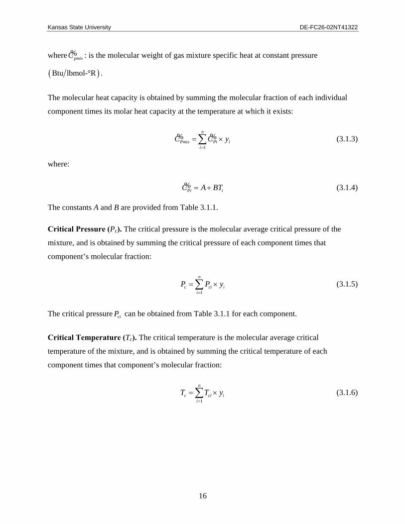
where pmixC% : is the molecular weight of gas mixture specific heat at constant pressure
( )Btu lbmol-°R .
The molecular heat capacity is obtained by summing the molecular fraction of each individual
component times its molar heat capacity at the temperature at which it exists:
1
n
Pmix Pi ii
C C y=
= ×∑% % (3.1.3)
where:
Pi iC A BT= +% (3.1.4)
The constants A and B are provided from Table 3.1.1.
Critical Pressure (Pc). The critical pressure is the molecular average critical pressure of the
mixture, and is obtained by summing the critical pressure of each component times that
component’s molecular fraction:
1
n
c ci ii
P P y=
= ×∑ (3.1.5)
The critical pressure ciP can be obtained from Table 3.1.1 for each component.
Critical Temperature (Tc). The critical temperature is the molecular average critical
temperature of the mixture, and is obtained by summing the critical temperature of each
component times that component’s molecular fraction:
1
n
c ci ii
T T y=
= ×∑ (3.1.6)

Kansas State University DE-FC26-02NT41322
17
Isentropic Exponents ( )σ . The isentropic exponent is obtained by:
1
1p
v av
p av
v
CC K
C KC
σ =
⎛ ⎞ −⎜ ⎟ −⎝ ⎠ =⎛ ⎞⎜ ⎟⎝ ⎠
(3.1.7)
The isentropic exponent is evaluated at the average temperature between two nodes:
Table 3.1.1: Constants for molar heat capacity (Ludwig 1983).
Gas Formula Molecular
Weight
Critical Pressure
(psia)
Critical Temperature
(°R) A BAir 28.97 546.70 238.4 6.737 0.000397Ammonia NH3 17.03 1,638.00 730.1 6.219 0.004342Carbon Dioxide CO2 44.01 1,073.00 547.7 6.075 0.005230Carbon Monoxide CO 28.01 514.40 241.5 6.780 0.000327Hydrogen H2 2.016 305.70 72.5 6.662 0.000417Hydrogen Sulfide H2S 34.07 1,306.00 672.4 7.197 0.001750Nitrogen N2 28.02 492.30 226.9 6.839 0.000213Oxygen O2 32.00 730.40 277.9 6.459 0.001020Sulfur Dioxide SO2 64.06 1,142.00 774.7 Water H2O 18.02 3,200.00 1,165.0 7.521 0.000926Methane CH4 16.04 673.10 343.2 4.877 0.006773Acetylene C2H2 26.04 911.20 563.2 6.441 0.007583Ethene C2H4 28.05 748.00 509.5 3.175 0.013500Ethane C2H6 30.07 717.20 549.5 3.629 0.016767Propene C3H6 42.08 661.30 656.6 4.234 0.020600Propane C3H8 44.09 617.40 665.3 3.256 0.0267331-Butene C4H8 56.11 587.80 752.2 5.375 0.029833Isobutene C4H8 56.11 580.50 736.7 6.066 0.028400Butane C4H10 58.12 530.70 765.3 6.188 0.032867Isobutane C4H10 58.12 543.80 732.4 4.145 0.035500Amylene C5H10 70.13 593.70 853.9 7.980 0.036333Isoamylene C5H10 70.13 498.20 836.6 7.980 0.036333Pentane C5H12 72.15 485.00 846.7 7.739 0.040433Isopentane C5H12 72.15 483.50 829.7 5.344 0.043933Neopentane C5H12 72.15 485.00 822.9 4.827 0.045300Benzene C6H6 78.11 703.90 1,011.0 -0.756 0.038267Hexane C6H14 86.17 433.50 914.3 9.427 0.047967Heptane C7H16 100.20 405.60 976.8 11.276 0.055400
Kansas State University DE-FC26-02NT41322
18
( )50 300 50
( ) ( ) 502250av
T i T j
K K K K
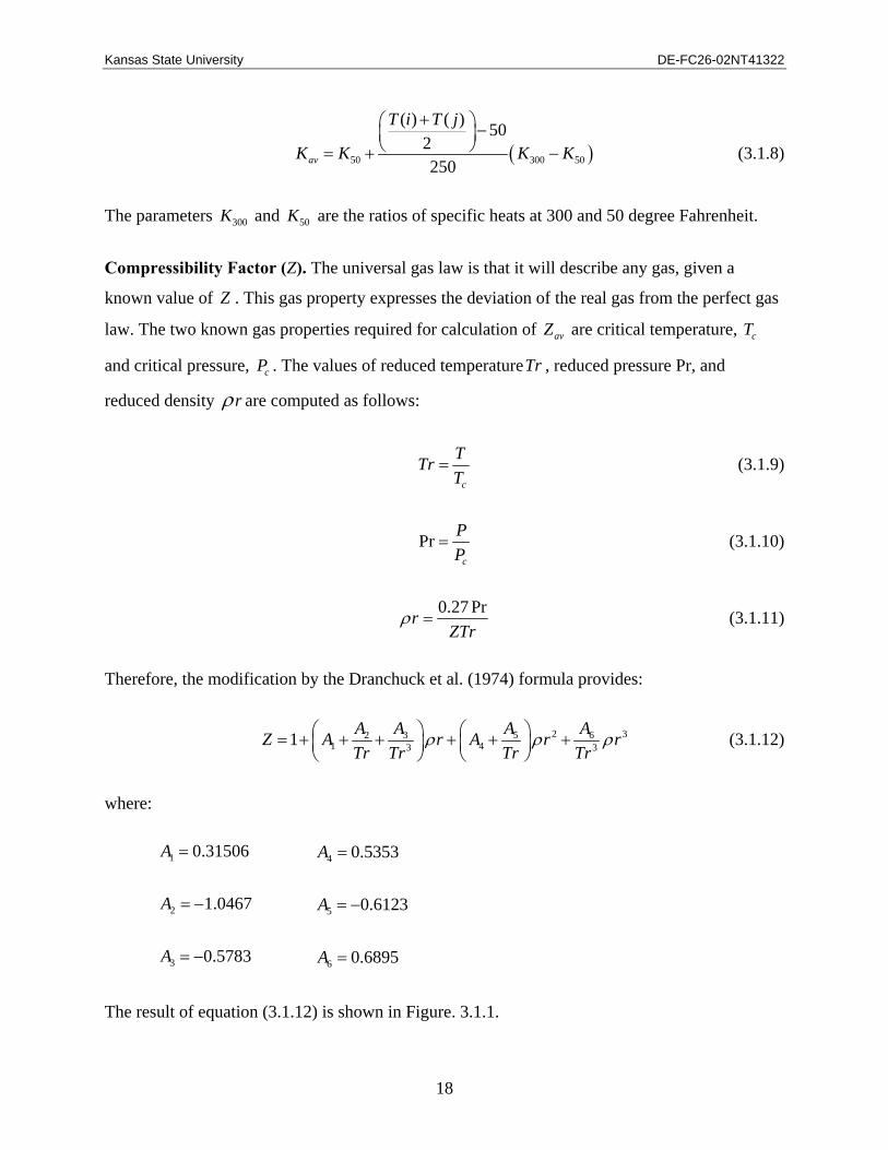
+⎛ ⎞ −⎜ ⎟⎝ ⎠= + − (3.1.8)
The parameters 300K and 50K are the ratios of specific heats at 300 and 50 degree Fahrenheit.
Compressibility Factor (Z). The universal gas law is that it will describe any gas, given a
known value of Z . This gas property expresses the deviation of the real gas from the perfect gas
law. The two known gas properties required for calculation of avZ are critical temperature, cT
and critical pressure, cP . The values of reduced temperatureTr , reduced pressure Pr, and
reduced density rρ are computed as follows:
c
TTrT
= (3.1.9)
Prc
PP
= (3.1.10)
0.27 PrrZTr
ρ = (3.1.11)
Therefore, the modification by the Dranchuck et al. (1974) formula provides:
2 33 5 621 43 31 A A AAZ A r A r r
Tr Tr Tr Trρ ρ ρ⎛ ⎞ ⎛ ⎞= + + + + + +⎜ ⎟ ⎜ ⎟
⎝ ⎠ ⎝ ⎠ (3.1.12)
where:
1
2
3
0.31506
1.0467
0.5783
A
A
A
=
= −
= −
The result of equation (3.1.12) is shown in Figure. 3.1.1.
4
5
6
0.5353
0.6123
0.6895
A
A
A
=
= −
=

Kansas State University DE-FC26-02NT41322
19
Lower Heating Value (LHV). The lower
heating value is obtained by:
( )1
n
iii
LHV LHV y=
= ×∑ (3.1.13)
The parameter LHV is the lower heating
value for each component ( )kJkg .
The non-isothermal flow of natural gas in
pipelines is governed by the time-dependent
continuity, momentum, and energy
equations, and an equation of state for
homogeneous, geometrically one-dimensional flow. By solving these equations, the behavior of
gas parameters can be obtained along the pipe network.
Issa and Spalding (1972), Deen and Reintsema (1983), Thorley and Tiley (1987), and Price et al.
(1996) developed the basic equations for one-dimensional, unsteady, compressible flow that
include the effects of wall friction and heat transfer:
Continuity Equation
( ) 0vt xρ ρ∂ ∂+ =
∂ ∂ (3.1.14)
Momentum Equation
v v P wv gsint x x A
ρ ρ ρ θ∂ ∂ ∂+ + = − −
∂ ∂ ∂ (3.1.15)
where 8
f v vw D
ρπ= .
Reduced Pressure (Pr)
Com
pres
sibi
lity
Fact
or(Z
)
0 0.2 0.4 0.6 0.8 1 1.2 1.4 1.6 1.80
0.1
0.2
0.3
0.4
0.5
0.6
0.7
0.8
0.9
1
Tr=.65
.85 .91.00
1.04 1.061.10
1.12
1.16
1.25
1.50
2
Fig. 3.1.1: Compressibility factor.

Kansas State University DE-FC26-02NT41322
20
Conservation of Energy
h h P P wvv vt x t x A
ρ ρ∂ ∂ ∂ ∂ Ω ++ − − =
∂ ∂ ∂ ∂ (3.1.16)
The term Ω is the heat flow into the pipe per unit length of pipe per unit time.
Equation of State
P ZRTρ= (3.1.17)
To obtain the enthalpy h in terms of P , Z , and T , Zemansky (1968) described the
thermodynamic identity:
1P
T dPdh CpdTTρ
ρ ρ⎧ ⎫∂⎛ ⎞= + +⎨ ⎬⎜ ⎟∂⎝ ⎠⎩ ⎭
(3.1.18)
The resulting set of equations is:
2
2 1ww
P
VP P v T Z wvv Vt x x CpT Z T A
ρ⎡ ⎤∂ ∂ ∂ ∂ Ω +⎛ ⎞ ⎛ ⎞ ⎛ ⎞ ⎛ ⎞+ + = +⎜ ⎟ ⎜ ⎟ ⎜ ⎟ ⎜ ⎟⎢ ⎥∂ ∂ ∂ ∂⎝ ⎠ ⎝ ⎠ ⎝ ⎠ ⎝ ⎠⎣ ⎦
(3.1.19)
1v v P wv gsin
t x x Aθ
ρ ρ∂ ∂ ∂⎛ ⎞ ⎛ ⎞ ⎛ ⎞+ + = − −⎜ ⎟ ⎜ ⎟ ⎜ ⎟∂ ∂ ∂⎝ ⎠ ⎝ ⎠ ⎝ ⎠
(3.1.20)
2 2
1 1w w
P T
V VT T T Z v P Z wvvt x Cp Z T x CpP Z P A
⎡ ⎤ ⎡ ⎤∂ ∂ ∂ ∂ ∂ Ω+⎛ ⎞ ⎛ ⎞ ⎛ ⎞ ⎛ ⎞ ⎛ ⎞+ + + = −⎜ ⎟ ⎜ ⎟ ⎜ ⎟ ⎜ ⎟ ⎜ ⎟⎢ ⎥ ⎢ ⎥∂ ∂ ∂ ∂ ∂⎝ ⎠ ⎝ ⎠ ⎝ ⎠ ⎝ ⎠ ⎝ ⎠⎣ ⎦ ⎣ ⎦ (3.1.21)
The parameter wV is:
2
1 1w
T P
ZRTVP Z P T ZZ P CpT Z Tρ
=⎧ ⎫⎡ ⎤∂ ∂⎪ ⎪⎛ ⎞ ⎛ ⎞− − +⎨ ⎬⎜ ⎟ ⎜ ⎟⎢ ⎥∂ ∂⎝ ⎠ ⎝ ⎠⎣ ⎦⎪ ⎪⎩ ⎭
(3.1.22)

Kansas State University DE-FC26-02NT41322
21
The continuity, momentum, and energy equations can then be written in terms of the mass flow
rate, m&. This is a matter of convenience since the primary interest, in this case, is the mass flow
rate as a function of time and location. This is accomplished by replacing the velocity with the
mass flow rate:
ZRTv
A PAm mρ
= =& &
(3.1.23)
Therefore:
2
2 1 11 1 1ww
T P
VP ZRT P Z P m T Z TVt PA ZRT Z P x x T Z T x
m mm
⎡ ⎤ ⎛ ⎞⎛ ⎞ ⎛ ⎞∂ ∂ ∂ ∂ ∂ ∂⎛ ⎞ ⎛ ⎞+ − − + + +⎜ ⎟⎢ ⎥⎜ ⎟ ⎜ ⎟⎜ ⎟ ⎜ ⎟∂ ∂ ∂ ∂ ∂ ∂⎝ ⎠ ⎝ ⎠⎝ ⎠ ⎝ ⎠⎣ ⎦ ⎝ ⎠
&& &&
2
21w
P
V T Z ZRT wCpT Z T A PA
m⎧ ⎫∂ Ω⎛ ⎞ ⎛ ⎞= + +⎨ ⎬⎜ ⎟ ⎜ ⎟∂⎝ ⎠ ⎝ ⎠⎩ ⎭
& (3.1.24)
2 1 1
T P
ZRT ZRT P Z P ZRT P P T ZPAP t PA x Z P t PA x T Z T
m m m m mm⎧ ⎛ ⎞ ⎛ ⎞∂ ∂ ∂ ∂ ∂ ∂⎪ ⎛ ⎞ ⎛ ⎞ ⎛ ⎞ ⎛ ⎞+ − − × + + +⎨ ⎜ ⎟ ⎜ ⎟⎜ ⎟ ⎜ ⎟ ⎜ ⎟ ⎜ ⎟∂ ∂ ∂ ∂ ∂ ∂⎝ ⎠ ⎝ ⎠ ⎝ ⎠ ⎝ ⎠⎪ ⎝ ⎠ ⎝ ⎠⎩
& & & & &&
ZRT P wZRT
gsinP x PA
T ZRT Tt PA x
mθ
∂+ = − −
∂
∂ ∂ ⎫⎛ ⎞× + ⎬⎜ ⎟∂ ∂⎝ ⎠⎭
& (3.1.25)
2
21 1w
P T
VT T Z ZRT P Z P ZRTPt Cp Z T AP x Z P x PA
m mm⎛ ⎞ ⎛ ⎞∂ ∂ ∂ ∂ ∂⎛ ⎞ ⎡ ⎛ ⎞ ⎤+ + − − +⎜ ⎟ ⎜ ⎟⎜ ⎟ ⎜ ⎟⎢ ⎥∂ ∂ ∂ ∂ ∂⎝ ⎠ ⎣ ⎝ ⎠ ⎦⎝ ⎠ ⎝ ⎠
& &&
22 2
1 1 1w w
P T
V VT Z T P ZCpT Z T x CpP Z P
⎛ ⎞⎛ ⎞ ⎧ ⎫∂ ∂ ∂⎛ ⎞ ⎛ ⎞⎜ ⎟× + + = −⎨ ⎬⎜ ⎟⎜ ⎟ ⎜ ⎟⎜ ⎟∂ ∂ ∂⎝ ⎠ ⎝ ⎠⎝ ⎠ ⎩ ⎭⎝ ⎠2
mZRT wA PAΩ⎛ ⎞+⎜ ⎟
⎝ ⎠
& (3.1.26)
Complete details about the derivation of these formulas and the specification of the initial values
for solving them are presented in Appendix A.

Kansas State University DE-FC26-02NT41322
22
Several investigators have developed various numerical schemes such as the method of
characteristics, the finite elements method, the explicit finite difference method, and the implicit
finite difference method. The choice depends partly upon the particular requirement of the
system under investigation. In this project we use the implicit finite difference method (Chapman
et al., 2003).
The major advantage of using an implicit method over the explicit method is that the implicit
method is unconditionally stable and imposes no restrictions on the maximum allowable time
step. The method, however, can yield unsatisfactory results for sharp transients. In addition,
some implicit methods have been known to produce erratic results during the imposition of some
types of boundary conditions (Thorley, 1987).
Whereas the explicit finite difference methods are forward difference methods, the fully implicit
method is a backward difference method. This method is unconditionally stable. Mohitpour et al.
(1996) and Kiuchi (1994) used this method to solve the continuity and momentum equations for
a gas pipeline network. This method is very accurate for the gas pipeline industry because their
problems usually involve relativity slow transients, and rapidly occurring phenomena are of far
less importance than long-term transients (Kiuchi, 1994).
The implicit method guarantees stability for a large time step, but requires using the Newton-
Raphson method to solve a set of nonlinear simultaneous equations at each time step.
For this study, the fully implicit method is used to solve the continuity, momentum, and energy
equations, and the results are compared with Kiuchi (1994). The fully implicit method consists of
transforming equations (3.1.24), (3.1.25), and (3.1.26) from partial differential equations to
algebraic equations by using finite difference approximations for the partial derivatives. Figure
(3.1.2) shows the mesh used in this
transformation. The pipe has N nodes and n
time levels.
Then:
x∆
1 2 3 i-1 i i+1 N
x∆
t∆
n+1
n
Fig. 3.1.2: Mesh of the solution.

Kansas State University DE-FC26-02NT41322
23
( )1 1
1 1
2
n n n ni i i iP P P PP
t t
+ ++ ++ − −∂
=∂ ∆
(3.1.27)
( )1 1
1 1
2
n n n ni i i i
t tm m m mm + +
+ ++ − −∂=
∂ ∆
& & & && (3.1.28)
( )1 1
1 1
2
n n n ni i i iT T T TT
t t
+ ++ ++ − −∂
=∂ ∆
(3.1.29)
So,
1 1
1n n
i iP PPx x
+ ++ −∂
=∂ ∆
(3.1.30)
1 1
1n ni i
x xm mm + +
+ −∂=
∂ ∆& &&
(3.1.31)
1 1
1n n
i iT TTx x
+ ++ −∂
=∂ ∆
(3.1.32)
and
1 1
1
2
n ni iP PP+ +
+ += (3.1.33)
1 1
1
2
n ni im mm+ ++ +
=& && (3.1.34)
1 1
1
2
n ni iT TT+ +
+ += (3.1.35)
Substituting equations (3.1.27) through (3.1.35) into equations (3.1.24), (3.1.25) and (3.1.26)
results in three sets of equations for each node and without considering node N there will be (3N-
3) equations for a pipe. The number of unknown values at time 1n + , which consists of pressure,
temperature and mass flow rate at each node, is 3N. Three equations will come from the

Kansas State University DE-FC26-02NT41322
24
boundary condition, and then there are 3N unknowns and 3N equations. These equations are
completely nonlinear and the Newton-Raphson method can be applied to solve these equations
for the compressible, non-isothermal transient flows through a pipe.
Kiuchi (1994) applied the fully implicit finite difference method to the isothermal formulation of
the conservation equations:
2
0wVPt A x
m∂ ∂+ =
∂ ∂& (3.1.36)
2 2 2
2 2 2
1 02
w w
w
m V fVm P Pg sinA t x PA x DA P V
m mθ
⎛ ⎞ ⎛ ⎞∂ ∂ ∂+ + + + =⎜ ⎟ ⎜ ⎟∂ ∂ ∂⎝ ⎠ ⎝ ⎠
&& & & (3.1.37)
The speed wV is ZRT . The first and second terms in the momentum equation (3.1.37) are the
inertia terms. Kiuchi, assuming a small flow velocity compared to the wave speed, neglected the
second term. In order to compare the model described in this study with the results presented by
Kiuchi (1994), the following adjustments were made:
1) The second inertia term was temporarily set to zero; and
2) The flow field was treated as isothermal, so the friction factor was assumed to be
constant with a value of 0.008.
The comparison uses the system described by Kiuchi (1994). This system is modeled as a simple
straight line 5 km in length, having an internal diameter 500 mm, and holding a gas of molecular
weight 18.0 at a pressure of 5 Mpa as shown in Figure 3.1.3. As the outlet valve opens, and the
out flow increases from zero to 300,000 m3/hr, flow rate m3/hr is shown in the standard condition
(100 KPa, 288.15 K), while the inlet pressure is maintained at 5 MPa. After maintaining this
condition for 20 min, the outlet valve closes. Solutions are performed using different grid
densities (5, 10, 20, 30, 40, 50, 60…) to ensure a grid independent solution. A grid density of 50
is found to be sufficient for this particular problem. Figures 3.1.4 and 3.1.5 show the variation in
flow at the center of the pipe length with respect to the number of nodes for the conditions given

Kansas State University DE-FC26-02NT41322
25
above. This is done at two different times (11
min and 31 min) and the results provide good
guidance for finding a suitable node (grid)
density for use in the solution process.
Figures 3.1.6 through 3.1.8 compare the
results from the current study to those from
the Kiuchi Model. Kiuchi compared his
method with the Crank-Nicolson method, the
method of characteristics, the Lax-Wendroff
method, and Guy’s method. The Crank-
Nicholson method gave an unstable solution
in the case of a large time step. The Lax-
Wandroff method and the method of
characteristics use the explicit method and gave a correct solution when the pipes were divided
into sufficiently small sections for both rapid and slow transient phenomena; however, both
required significant computation time. Kiuchi (1994) showed that Guy’s method, which uses the
implicit method, has good stability for a small time step and has greatly dampened oscillations.
1 2 50. . . .
5 Km
500 mm
49Q
(50)
0
300,000
3m hr
0 10 30 60minTime
Node
Fig. 3.1.3: Pipe information and boundary condition for flow through the valve.
Number of Node
Flow
(m3 /h
)*10
5
10 20 30 40 50 602.5
2.6
2.7
2.8
2.9
3
Dt= 60 sec
Dt=6 sec
Fig. 3.1.4: Variation of flow at center of pipe length at time 11 min with respect to number of nodes for isothermal condition.
Number of Node
Flow
(m3 /h
)*10
5
10 20 30 40 50 600
0.05
0.1
0.15
0.2
0.25
0.3
0.35
0.4Dt= 60 sec
Dt= 6 sec
Fig. 3.1.5: Variation of flow at center of pipe length at time 31 min with respect to number of nodes for isothermal condition.

Kansas State University DE-FC26-02NT41322
26
Time(min)
Flow
(m3 /h
)*10
5
0 10 20 30 40 50 60-1-0.5
00.5
11.5
22.5
33.5
4
(a) (b)
Fig. 3.1.6: Comparison of present work (a) with Kiuchi model (b) for ∆t = 1.0 min.
Time(min)
Flow
(m3 /h
)*10
5
0 10 20 30 40 50 60-1-0.5
00.5
11.5
22.5
33.5
4
(a) (b)
Fig. 3.1.7: Comparison of present work (a) with Kiuchi model (b) for ∆t = 0.1 min.
Time (min)
Flow
(m3 /h
)*10
5
0 10 20 30 40 50 60-1-0.5
00.5
11.5
22.5
33.5
4
(a) (b)
Fig. 3.1.8: Comparison of present work (a) with Kiuchi model (b) for ∆t = 0.01 min.

Kansas State University DE-FC26-02NT41322
27
Figures 3.1.6, 3.1.7 and 3.1.8 show the variation of flow rates at node 1 (pipe inlet) with respect
to time for different time steps. As shown, the results of the present work compare very closely
to the Kiuchi solutions. As the time step decreases, the flow rate oscillation at this condition
increases. Eventually this oscillation is damped due to conservation of mass.
The Kiuchi study neglected the second term (the inertia term) of equation (3.1.37) and assumed a
uniform and constant friction factor. The present study investigates the effect of the inertia term
as well as friction variation. Figures 3.1.9, 3.1.10, 3.1.11 and 3.1.12 show the effect of the time
step on the flow rate at node 1 and the effect of pressure changes at all nodes.
During valve opening and closing, all the gas properties attempt to change due to the condition
change. The system requires some finite time to adjust itself to the new condition and reach
steady state. However, different types of behaviors take place before the flow reaches the steady
condition, as shown at different time steps in Figures 3.1.9, 3.1.10, 3.1.11, and 3.1.12. For a large
time step, the small effect of some parameters such as the inertia term may not be noticeable
within the flow before it reaches the steady state condition. In this case, the effect of the inertia
term simply vanishes between the time steps, as Figures 3.1.9 and 3.1.10 depict. Therefore, the
existence or absence of the inertia term in the momentum equations will not affect the results. On
the other hand, for small time steps the effect of this parameter is noticeable and in fact plays an
important rule in the fluctuations in amplitude and in damping before reaching steady state, as
shown in Figures 3.1.11 and 3.1.12.
Time(min)
Flow
(m3 /h
)*10
5
0 10 20 30 40 50 60-1-0.5
00.5
11.5
22.5
33.5
4
Time(min)
Pre
ssur
e(M
Pa)
0 10 20 30 40 50 604.9
4.92
4.94
4.96
4.98
5
5.02
5.04
Node 50
Node 1
(a) (b) Fig 3.1.9: Solution for isothermal model including inertia term with ∆t = 1.0 min.

Kansas State University DE-FC26-02NT41322
28
Time(min)
Flow
(m3 /h
)*10
5
0 10 20 30 40 50 60-1-0.5
00.5
11.5
22.5
33.5
4
Time(min)
Pre
ssur
e(M
Pa)
0 10 20 30 40 50 604.9
4.92
4.94
4.96
4.98
5
5.02
5.04
Node 50
Node 1
(a) (b) Fig 3.1.10: Solution for isothermal model including inertia term with ∆t = 0.1 min.
Time (min)
Flow
(m3 /h
)*10
5
0 10 20 30 40 50 60-1-0.5
00.5
11.5
22.5
33.5
4
Time (min)
Pre
ssur
e(M
Pa)
0 10 20 30 40 50 604.9
4.92
4.94
4.96
4.98
5
5.02
5.04
Node 1
Node 50
(a) (b) Fig 3.1.12: Solution for isothermal model including inertia term with ∆t = 0.01 min.
Time(min)
Flow
(m3 /h
)*10
5
0 10 20 30 40 50 60-1-0.5
00.5
11.5
22.5
33.5
4
Time(min)
Pre
ssur
e(M
Pa)
0 10 20 30 40 50 604.9
4.92
4.94
4.96
4.98
5
5.02
5.04
Node 50
Node 1
(a) (b) Fig 3.1.11: Solution for isothermal model including inertia term with ∆t = 1 sec.

Kansas State University DE-FC26-02NT41322
29
The energy equation (3.1.26), which is coupled to the momentum and continuity equations, is
used to account for the temperature variation along the pipe. Specifically, the governing
equations are solved using the fully implicit method. The mass flow rate and pressure boundary
conditions are similar to the isothermal case.
Figure 3.1.13 shows the temperature boundary condition for the inlet flow as the valve is opened.
The equivalent heat transfer coefficient between the pipe and its surroundings is 200 W/ m2K.
The effects of non-isothermal conditions on the flow are illustrated in Figures 3.1.14 through
3.1.19. Figures 3.1.14, 3.1.16, and 3.1.18 show the effect of the time step on the flow rate at node
1 at different times. Figures 3.1.15, 3.1.17, and 3.1.19 show the same effect on the temperature
and compressibility variation. The figures show that the flow rate is significantly affected by the
temperature variations until the flow reaches steady state. While the mass flow rate in the
isothermal case suddenly jumps to the steady state condition, the mass flow rate of the non-
isothermal case gradually increases until steady state is reached. This occurs because the density
varies with respect to temperature. By opening and closing the valve, the flow pressure and
temperature change. This results in a significant density change. As the density change slowly
transfers from one part of the flow to the other parts, the properties of the flow change
accordingly. Hence, the temperature effect on the pipeline flow analysis must be taken into
account since ambient conditions vary not only along with the seasons, but also between day and
night time.
Tem
pera
ture
at n
ode
1
298.18
0 10 30Time
333.18
(K)
60 min
Fig 3.1.13: Temperature boundary condition at node 1.

Kansas State University DE-FC26-02NT41322
30
Time(min)
Flow
(m3 /h
)*10
5
0 10 20 30 40 50 60-1-0.5
00.5
11.5
22.5
33.5
4
Time(min)
Pre
ssur
e(M
Pa)
0 10 20 30 40 50 604.9
4.92
4.94
4.96
4.98
5
5.02
5.04
Node 50
Node 1
(a) (b)
Fig 3.1.14: Flow (a) and Pressure distribution (b) for non-isothermal condition and ∆t = 1.0 min.
Time(min)
Tem
pera
ture
(K)
0 10 20 30 40 50 60280
290
300
310
320
330
340Node 1
Node 50
Time(min)
Com
pres
sibi
lity
fact
or(Z
)
0 10 20 30 40 50 600.76
0.78
0.8
0.82
0.84
0.86
0.88 Node 1
Node 50
(a) (b)
Fig 3.1.15: Temperature (a) and Compressibility factor (b) for non-isothermal condition and ∆t = 1.0 min.
Time(min)
Flow
(m3 /h
)*10
5
0 10 20 30 40 50 60-1-0.5
00.5
11.5
22.5
33.5
4
Time(min)
Pre
ssur
e(M
Pa)
0 10 20 30 40 50 604.9
4.92
4.94
4.96
4.98
5
5.02
5.04
Node 1
Node 50
(a) (b)
Fig 3.1.16: Flow (a) and Pressure distribution (b) for non-isothermal condition and ∆t = 0.1 min.

Kansas State University DE-FC26-02NT41322
31
Time(min)
Tem
pera
ture
(K)
0 10 20 30 40 50 60280
290
300
310
320
330
340Node 1
Node 50
Time(min)
Com
pres
sibi
lity
fact
or(Z
)
0 10 20 30 40 50 600.76
0.78
0.8
0.82
0.84
0.86
0.88 Node 1
Node 50
(a) (b)
Fig 3.1.17: Temperature (a) and compressibility factor (b) for non-isothermal condition and ∆t = 0.1 min.
Time(min)
Flow
(m3 /h
)*10
5
0 10 20 30 40 50 60-1-0.5
00.5
11.5
22.5
33.5
4
Time(min)
Pre
ssur
e(M
Pa)
0 10 20 30 40 50 604.9
4.92
4.94
4.96
4.98
5
5.02
5.04
Node 50
Node 1
(a) (b)
Fig. 3.1.18: Flow (a) and pressure distribution (b) for non-isothermal condition and ∆t = 1.0 sec.
Time(min)
Tem
pera
ture
(K)
0 10 20 30 40 50 60280
290
300
310
320
330
340Node1
Node 50
Time(min)
Com
pres
sibi
lity
fact
or(Z
)
0 10 20 30 40 50 600.76
0.78
0.8
0.82
0.84
0.86
0.88 Node 1
Node 50
(a) (b)
Fig. 3.1.19: Temperature (a) and compressibility factor (b) for non-isothermal condition and ∆t = 1.0 sec.

Kansas State University DE-FC26-02NT41322
32
The flow rate and pressure variation with respect to pipe length and time are shown in Figure
3.1.20. As the length of pipe increases, the pressure drop due to the opening of the valve
increases. A longer time is required to reach a steady state condition. Similarly, when the valve is
closed, the pressure takes longer to reach the final value for longer pipe lengths. Therefore, pipes
with longer lengths do not experience sudden pressure changes. The flow rate behaves similarly.
Subtask 1.2: Compressor Station Node
The compressor station is somewhat more complex than the pipeline node since there can be
several different configurations of engines, gas turbines, and compressors. To complicate the
problem, one or more engines may operate at part-load. The compressor station node is further
subdivided into additional subnodes, with each subnode representing a reciprocating engine, gas
turbine, centrifugal compressor, or reciprocating gas compressor.
Reciprocating Engine Submodel. Prior research has resulted in the development of a robust
turbocharger-reciprocating engine computer simulation (T-RECS) package (Chapman and
Keshavarz-Valian, 2003), which model uses energy, momentum, and mass conservation
equations to conduct a cycle analysis of the gases within the engine cylinder. It calculates the
airflow rate through the engine system, the exhaust gas temperature, the power generated by the
engine, and fuel consumed by the engine. The simulation completes a cycle analysis that
Time (min)
Flow
(m3 /h
)*10
5
0 60 120 180 240 300-1-0.5
00.5
11.5
22.5
33.5
4
10 Km
100 Km
100 Km
10 Km
Time (min)
Pre
ssur
e(M
pa)
0 50 100 150 200 250 300
4
4.2
4.4
4.6
4.8
5 10 Km
100 Km
(a) (b)
Fig. 3.1.20: Flow distribution in the head of pipe (a) and pressure distribution in the end of pipe (b) for different pipe length respect to time.

Kansas State University DE-FC26-02NT41322
33
calculates the in-cylinder pressure and temperature throughout the engine cycle. The T-RECS
program was funded by the Gas Research Institute (now the Gas Technology Institute) and was
validated with information from the Pipeline Research Council International, Inc.
Inputs to this simulation can be as detailed as the specification of the spark advance for the spark
plug, or as easy as the selection of a generic 2- or 4-stroke cycle engine that generates a
particular power output. Since the computational effort is of the order of 50 seconds, the engine
subnode will present only a small addition to the computational effort necessary for the entire
VPST.
Gas Turbine Submodel. As with the reciprocating engine node, the goal of the gas turbine
engine node is to provide estimates of power, exhaust gas temperature, fuel consumption, and
emissions. These inputs are based on operating conditions and the specific design of the gas
turbine. Euler’s equations for turbomachinery, velocity triangles, and combustion analysis are
used to determine the gas turbine output conditions (Mattingly, 1999). The combination of
Euler’s equations and velocity triangles provides a balance between the conservation of energy
and angular momentum. Empirical relationships allow compressor and turbine efficiencies to be
incorporated into the model.
Centrifugal Compressor Submodel. The compressor equations are used for two types of
solutions. One solution type is to define pipeline conditions across the compressor (flow,
discharge pressure, suction pressure, and suction temperature) with the goal to determine
whether the operating point is on the compressor map and, if so, to determine the fuel
consumption of the driver (gas turbine, engine). The other solution type is the specification of the
driver to operate at full load power, with the goal to determine the pressure ratio produced by the
compressor at a specified ratio.
The key parameters that are necessary to describe compressor performance are isentropic head,
isentropic efficiency, rotational speed and power. Considering suction, s , and discharge, d , for
the compressor shown in Figure 3.1.21 yields:
1s s d
s
T RZ PHeadP
σ
σ⎛ ⎞⎛ ⎞⎜ ⎟= −⎜ ⎟⎜ ⎟⎝ ⎠⎝ ⎠
(3.1.38)

Kansas State University DE-FC26-02NT41322
34
where:
Head Isentropic head
( )kJkg
sT Suction Temperature
(K)
sP Suction Pressure (Pa)
dP Discharge Pressure
(Pa)
TakingG
RRM
= and Gg
air
MM
γ = , results in:
0.28704 1s s d
g s
T Z PHeadP
σ
σγ
⎛ ⎞⎛ ⎞⎜ ⎟= −⎜ ⎟⎜ ⎟⎝ ⎠⎝ ⎠
(3.1.39)
The volumetric flow rate through the compressor is expressed in terms of the mass flow rate and
standard pressure and temperature is:
acst
sc
sc sc
m RQ PZ T
=&
(3.1.40)
where:
scP Standard Pressure (101,325 Pa)
scT Standard Temperature (288.15 K)
scZ 1.00
Discharge
Fuel consumption
Suction
Fig. 3.1.21: Schematic of compressor and fuel consumption.

Kansas State University DE-FC26-02NT41322
35
Then:
mech
ac
is
Head mPowerηη×
=&
(3.1.41)
where:
Power Power (Kw)
isη Isentropic efficiency
mechη Mechanical efficiency ( )~ 0.98
One method to input centrifugal compressor characteristics into a pipeline simulation model is to
digitize the entire head versus capacity and store it as a table. On the other hand, a simplified but
still accurate representation of the head versus capacity curve, however, can be obtained through
the use of normalized characteristics. Figure 3.1.22 shows a sample compressor map.
Three normalized parameters can be used to describe a compressor map 2Head
N, acQ
N , and
isη . Using standard polynomial cure-fit
procedures for each centrifugal compressor
(Odom, 1990) relationships between these
three parameters are:
2
2 1 2 3ac acQ QHead
b b bN N N
+ += ⎛ ⎞ ⎛ ⎞⎜ ⎟ ⎜ ⎟⎝ ⎠ ⎝ ⎠
(3.1.42)
and:
2
54 6ac ac
isQ Qb b bN N
η +⎛ ⎞ ⎛ ⎞= + ⎜ ⎟ ⎜ ⎟⎝ ⎠ ⎝ ⎠
(3.1.43)
The parameters 1 2 3 4 5 6, , , , , and b b b b b b are
the coefficients of the centrifugal compressor Fig. 3.1.22: Compressor Map (Odom 1990).

Kansas State University DE-FC26-02NT41322
36
map that characterize a particular compressor. With these coefficients, the compressor speed and
isentropic efficiency can be calculated as functions of the isentropic head and inlet volumetric
flow.
The fuel consumption for the driver is obtained by:
dr
fPower
LHVm
η=
×& 3.1.44)
where:
fm& Fuel consumption ( )kgs
drη Efficiency of driver (engine or gas turbine)
The discharge temperature is obtained by:
1100s d
sdsis
PTT TP
σ
η⎡ ⎤⎛ ⎞⎢ ⎥= + −⎜ ⎟⎢ ⎥⎝ ⎠⎣ ⎦
(3.1.45)
The mass balance between suction and discharge of the compressor is:
) )s dac ac fm m m= +& & & (3.1.46)
where fm& is the fuel consumed by the compressor-engine system.
Reciprocating Gas Compressor Submodel.
Reciprocating gas compressors are somewhat
more complicated than the centrifugal
compressors. Figure 3.1.23 illustrates the
working mechanisms of a reciprocating
compressor. These compressors generally
contain unloading pockets that can be opened
and closed to decrease or increase the
compressor load. Reciprocating compressors
are positive displacement machines that Fig. 3.1.23: Schematic of reciprocating compressor.

Kansas State University DE-FC26-02NT41322
37
increase air pressure by reducing volume. Substantial information exists on methods to
determine various performance factors of these compressors, such as the power required and the
temperature and pressure rise across the reciprocating compressors as functions of design and
operating conditions.
Figure 3.1.24 shows the p-V diagram for the ideal and actual processes in a reciprocating
compressor. Some information and definitions for this process are:
1. Volumetric efficiency (VE): the ratio of inlet volume to displacement
2. Cylinder clearance volume (CL): the volume of gas left in the cylinder at the discharge
end of the stroke, which includes the space between the piston and cylinder head, the
volume of the valves, valve pockets and any added clearance. Clearance volume is
Cle
aran
ce
Actual Capacity
Piston Displacement
Volume
Ps
Pd
Pressure
Ideal CycleActual Cycle
Discharge
Suction
Compression
Expansion
Disgharge ValveLoss Horsepower
Suction Valve LossHorsepower
Fig. 3.1.24: Reciprocating compressor P-V diagram for ideal and actual condition.

Kansas State University DE-FC26-02NT41322
38
generally expressed as a percentage of the swept volume of a given cylinder end.
3. Valve loss horsepower (VLHP): the power that created by the pressure drop encountered
as gas flows through the suction and discharge valve.
4. Adiabatic Horsepower (AHP): the power that created from p-V diagram for adiabatic
condition (Ideal) without considering valve loss regions.
The procedure to determine the horsepower consumed by a reciprocating compressor is:
1. Estimate suction volumetric efficiency (Ariel, 2001):
( ) 198
0.98 1100
c s ks c
d
R ZVE CL RZ
⎛ ⎞⎡ ⎤− ⎛ ⎞= − −⎜ ⎟⎢ ⎥⎜ ⎟⎜ ⎟⎝ ⎠⎣ ⎦⎝ ⎠
(3.1.47)
where:
CL Clearance
cR Compression ratio
2. Estimate suction volumetric efficiency (Ariel, 2001):
( ) 198
0.98 1100
c s ks c
d
R ZVE CL RZ
⎛ ⎞⎡ ⎤− ⎛ ⎞= − −⎜ ⎟⎢ ⎥⎜ ⎟⎜ ⎟⎝ ⎠⎣ ⎦⎝ ⎠
(3.1.47)
where:
CL Clearance
cR Compression ratio
sZ Compressibility factor at suction side condition
dZ Compressibility factor at discharge side condition
k Adiabatic exponent

Kansas State University DE-FC26-02NT41322
39
3. Estimate the discharge volumetric efficiency (Phillippi, 2002):
1
sD
s kc
d
VEVEZ RZ
=⎛ ⎞⎜ ⎟⎝ ⎠
(3.1.48)
4. Estimate the adiabatic horsepower (Phillippi, 2002):
( ) ( )( )( )( ) ( )
( ) ( )( ) ( )( )1144
133000 1 2
ks s s d k
cs
K P PD VE Z ZAHP R
k Z
−+ ⎡ ⎤= −⎢ ⎥− × ⎣ ⎦
(3.1.49)
where sP is the suction pressure (psia). The piston displacement is defined as (Ariel,
2001):
1728
SweptV NPD
×= (3.1.50)
where N is the rotational speed of the compressor crankshaft (rpm). The swept volume
that is used in equation (1-50) is defined as:
Swept HE CEV V V= + (3.1.51)
where:
HE PV A S= ×
CE P RV A S A S= × − ×
HEV Head end volume (in3)
CEV Crank end Volume (in3)
PA Piston area (in2)
RA Rod area (in2)

Kansas State University DE-FC26-02NT41322
40
S Stroke (in)
5. Estimate the suction valve loss horsepower (Phillippi, 2002):
( )( )( )s P sSVLHP P A VE S N= ∆ × (3.1.52)
where sP∆ is the pressure drop across the suction valve event.
6. Estimate the discharge valve loss horsepower (Phillippi, 2002):
( )( )( )d P dDVLHP P A VE S N= ∆ × (3.1.53)
where dP∆ is pressure drop into discharge valve event.
7. Estimate the compression efficiency (Phillippi, 2002):
mechAHP EAHP+SVLHP+DVLHPcE ×
= (3.1.54)
where mechE is the mechanical efficiency.
8. Estimate the indicated horsepower (Phillippi, 2002):
IHP AHP SVLHP DVLHP= + + (3.1.55)
9. Estimate brake horsepower:
mech c
IHPBHPE E
=×
(3.1.56)
10. Estimate mass fuel consumption from equation (3.1.44):
These equations that describe the performance of reciprocating and centrifugal compressors are
based on the assumption of a quasi-steady flow at each time step of the numerical solution.

Kansas State University DE-FC26-02NT41322
41
Compression Unit. A compression unit is defined as a combination of a compressor and its
driver. Four possible combinations are:
1. Reciprocating compressor driven by reciprocating engine
2. Centrifugal compressor driven by gas turbine
3. Reciprocating compressor driven by gas turbine
4. Centrifugal compressor driven by reciprocating engine
Items 1 and 2 are the most commonly found compression units in a natural gas pipeline system
and hence were the primary focus areas for modeling in this project. A compression unit could
be an integral type as many reciprocating engines and reciprocating compressor combinations are
Cle
aran
ce
Actual Capacity
Piston Displacement
Volume
Ps
Pd
Pressure
Ideal CycleActual Cycle
Discharge
SuctionCom
pression
Expansion
Disgharge ValveLoss Horsepower
Suction Valve LossHorsepower
Fig. 3.1.24: Reciprocating compressor P-V diagram for ideal and actual condition.

Kansas State University DE-FC26-02NT41322
42
or could be a non-integral type where the compressor is connected to the driver using an external
coupling. A comprehensive compression unit database supplements the individual submodels
described earlier. The user has the choice of choosing predefined units from the database or
creating new units by choosing appropriate submodels constrained by any one of the four
possible unit combinations. The primary data that the compression unit database includes are the
unit speed and the unit rated power. The individual driver and compressor submodel database
includes manufacturers’ basic data, operating information and modeling information. The
operating information includes the input parameters required for submodel simulation. The
modeling information consists of the coefficients obtained as a result of digitizing performance
data for both compressor and the driver.
Subtask 1.3: Blocking Valve Node
The blocking valve is modeled as a boundary condition for the network. Figure 3.1.25
schematically illustrates the blocking valve that is used for the simulation. When the valve is
open, the conservation of mass, energy, and momentum reduce to: 1 2m m=& & , 1 2P P= , and 1 2T T= .
When the valve is closed, the conservation of mass, energy, and momentum are not applicable
since there is no connection between the inlet and the outlet of valve. The mass flow rate at the
valve outlet at the time when the valve is closed is zero, however, mass continues to increase at
the valve entrance until a steady-state condition is reached. The equation, 2 0m =& , is used to
model the valve closing event.
Figure 3.1.26 shows a blocking valve that is positioned between two long pipes. Each 500 mm
diameter pipe is 50 km long. Each pipe is separated into 50 computational nodes. The constant
boundary conditions are:
• Inlet pressure at Pipe 1 (Point 1): 6
MPa
1 2
Fig. 3.1.25: Blocking valve.

Kansas State University DE-FC26-02NT41322
43
• Inlet temperature at Pipe 1 (Point 1): 333.33 K
• Outlet pressure at Pipe 2 (Point 4): 4 MPa
The valve is opened for 41 minutes and 40 seconds, after which the valve is suddenly closed.
The valve then remains closed for an additional 33 minutes, 20 seconds. At time = 75 minutes
the valve opens and remains open until the simulation is stopped.
Figure 3.1.27 shows the pressure distribution for various nodes ranging from Node 1 (inlet) to
Node 50 (exit). The pressure at each node reaches a steady state condition in the time period
when the valve is initially open. The pressure gradient between nodes 1 and 50 occurs due to the
frictional losses in the pipe. At time 41 minutes and 40 seconds when the valve closes, the
pressure at each computational node increases to reach to inlet pressure. At 75 minutes, when the
valve re-opens, the pressure at all computational nodes again trend to the steady state conditions.
A similar characteristic occurs in the pipe
downstream of the valve.
Figure 3.1.28 exhibits the mass flow rate
variation with respect to time for the
computational nodes along the inlet pipe that
is upstream of the blocking valve (Pipe 1).
Prior to closing the valve, the mass flow rate
at all nodes asymptotically approaches the
steady state flow rate of 112.6 kg/s. At time
41 minutes and 40 seconds the valve closes
and the mass flow rate at Node 50 (end of
pipe that is connected to the valve) suddenly
Time (min)
Pre
ssur
e(M
Pa)
25 50 75 100 1254
5
6
7
Node 1
Node 50
Pressure distribution for pipe 1
Fig. 3.1.27: Pressure distribution for inlet pipe (Pipe 1).
Pipe 11 2 3 4
Pipe 2
Fig. 3.1.26: Schematic of valve and two pipes connected.

Kansas State University DE-FC26-02NT41322
44
drops to zero. Since the fluid is
compressible, the flow rate at the upstream
nodes asymptotically approach zero,
essentially packing the pipe with gas. At
75 minutes, the blocking valve re-opens
and the mass flow rate at each
computational node again asymptotically
approach the steady state flow rate of
112.6 kg/s. Figure 3.1.29 illustrates the
similar characteristic for the down stream
section of pipe (Pipe 2).
Subtask 1.4: Regulator and Metering Station Node
The pressure regulator impacts VPST by
creating a prescribed down stream
pressure. The regulator is modeled in a
similar manner to the blocking valve, since
the conservation equations reduce to:
1 2m m=& & . 1 2P P≠ , and 1 2T T≅ .
Figure 3.1.30 schematically illustrates a
regulator that is positioned between two 5
km long, 500 mm diameter pipes to
control the pressure at the regulator outlet
pressure. Each pipe is separated into 20
nodes with the following time-invariant constant boundary conditions:
• Inlet pressure at Pipe 1 (Point 1): 6 MPa
• Inlet temperature at Pipe 1 (Point 1): 333.33 K
Time (min)
Mas
sflo
wra
te(k
g/s)
25 50 75 100 1250
50
100
150
200
250
Node 1
Node 1
Node 50
Node 50
Mass flow rate distribution for pipe 1
Fig. 3.1.28: Mass flow rate distribution for inlet pipe (Pipe 1).
Time (min)
Mas
sflo
wra
te(k
g/s)
25 50 75 100 1250
50
100
150
200
250
Node 1
Node 50
Node 1
Node 50
Mass flow rate distribution for pipe 2
Fig 3.1.29: Mass flow rate distribution for outlet pipe (Pipe 2).

Kansas State University DE-FC26-02NT41322
45
• Outlet pressure at regulator (Point 3): 4.5 MPa
• Outlet pressure at pipe 2 (Point 4): 3.5 MPa
Figure 3.1.31 shows the transient response of the mass flow rate in Pipe 1. As show in this
figure, the mass flow rate at different nodes exhibits a transient fluctuation until all nodes reach
the steady-state condition 10 minutes when the mass flow rate is 326.36 kg/s. The behavior is
similar in Pipe 2 (Figure 3.1.32) and after 10 minutes all mass flow rates reach steady-state
conditions.
Figures 3.1.33 and 3.1.34 illustrate the pressure distribution within the inlet and outlet pipes. The
pressure distribution for each node is different with respect to time due to the compressibility
effects and friction losses within the pipes. As shown in these figures, the node pressures
asymptotically approach the steady state pressure.
Pipe 11 2 3 4
Pipe 2
Fig. 3.1.30: Schematic of regulator and two pipes connected.
Time (min)
Mas
sflo
wra
te(k
g/s)
5 10 15 20 25240
260
280
300
320
340
360
Point 2
Point 1
Pipe 1
Fig. 3.1.31: Mass flow rate variation with respect to time at Pipe 1.
Time (min)
Mas
sflo
wra
te(k
g/s)
5 10 15 20 25300
320
340
360
Point 4
Point 3
Pipe 2
Fig. 3.1.32: Mass flow rate variation with respect to time at Pipe 2.

Kansas State University DE-FC26-02NT41322
46
At the end of simulation, the pressure at Point 1 becomes 5.27 MPa at Pipe 1. The same behavior
occurs at Pipe 2, but at this pipe the pressure at the inlet and outlet is fixed. Therefore there is no
transient variation in pressure for other nodes as shown in Figure 3.1.34.
The same type of information is depicted for the temperature distribution for inlet and outlet
pipes as shown in Figure 3.1.35 and Figure 3.1.36. Because of heat transfer between the pipe and
environment, the temperature at each node is different. After about 10 minutes, the temperature
at Point 2 becomes 321 K and 312 K at Point 4.
Time (min)
Pre
ssur
e(M
Pa)
5 10 15 20 254
5
6
7
Point 1
Point 2
Pipe 1
Fig. 3.1.33: Pressure distribution with respect to time in Pipe 1.
Time (min)
Pre
ssur
e(M
Pa)
5 10 15 20 253
3.5
4
4.5
5
Point 3
Point 4
Pipe 2
Fig. 3.1.34: Pressure distribution with respect to time in Pipe 2.
Time (min)
Tem
pera
ture
(K)
5 10 15 20 25290
300
310
320
330
340
Point 3
Point 4
Pipe 2
Fig. 3.1.36: Temperature distribution with respect to time at Pipe 1.
Time (min)
Tem
pera
ture
(K)
5 10 15 20 25290
300
310
320
330
340
Point 1
Point 2
Pipe 1
Fig. 3.1.35: Temperature distribution with respect to time at Pipe 1.

Kansas State University DE-FC26-02NT41322
47
Task 2.0: Develop Optimization Algorithm
The analysis and simulation tools developed under Task 1.0 are used as a foundation to
formulate new methods for performing optimization and reliability studies on the pipeline. This
allows VPST to function not only as an analysis tool, but also as a design and operational
planning tool. Based on interactions with industry personnel, three key needs were identified:
1. Develop optimal network performance methods through appropriate equipment selection
2. Develop methods to optimize the location and design of mid-station compression
3. Develop methods to optimize network reliability with respect to equipment failure.
It is worth noting that none of these capabilities are currently available, even though they are
highly desirable to the natural gas pipeline industry. In all the above optimizations, the goal is to
maximize gas flow while keeping losses within limits. Alternatively, losses may be minimized
subject to limits on flow rate. Clearly, this is a constrained optimization problem, and can be
solved as such. However, the industry routinely converts this to the roughly equivalent
unconstrained problem of maximizing the pressure in the pipeline. The original intention was to
support all of these optimization problem formulations. However, the project scope was later
redefined in consultation with industry representatives and DOE, and the focus of the
optimization was shifted to operational optimization, with particular emphasis on cost reduction
through minimization of fuel consumption. It is important to note that currently available
commercial packages do not provide the capability for fully automated optimization of
operational parameters; rather, they provide computational support for human decision making.
In other words, the current generation of software in this area allows a human operator to
simulate pipe flow in a network without detailed modeling of equipment such as compressors
and drivers. Any decisions on how to optimize the operation of equipment must be made by the
human operator based on simplified simulation of a few scenarios. Thus, the solutions that are
arrived at are generally not truly optimal, and require considerable user involvement. This study
advances this methodology in that the software, using detailed equipment modeling and rigorous
mathematical optimization, automatically generates truly optimal solutions with practically no
user involvement. This represents a significant advancement in the state-of-the-art in this field.

Kansas State University DE-FC26-02NT41322
48
The formulation and numerical solution scheme discussed earlier provides the ability to simulate
the behavior of the system under a variety of conditions. Thus, it provides the necessary analysis
capability to support optimization. In general, two types of optimization problems are of interest
in pipeline networks: design optimization and operation optimization. In design optimization, the
goal is to optimize the pipeline design by selecting appropriate layouts, equipment, etc. In
operation optimization, the network and station configuration is given, and the goal is to operate
the pipeline network in an optimal manner.
In this work, only operation optimization is considered. The optimal operation of a network
involves meeting all performance requirements that are placed on the network, while minimizing
an objective function. The operating parameters whose values can be adjusted to achieve this
optimal operating point are referred to as “design variables” in the optimization problem.
In order to optimize the operation of the network, the problem is formulated in the format of a
standard nonlinear programming problem (NLP). This standard form is:
Find the values of the design variables [b1,b2,….,br]T to:
Minimize an objective function f(b)
Subject to the constraints: hj(b) = 0 , j = 1,…, m
and gj(b) ≤ 0 , j = m+1,…,n
The formulation of the network operation problem in the standard NLP form must be done
carefully to ensure that the NLP formulation captures all the relevant aspects of the associated
network problem.
Formulation of the Optimization Problem. The formulation of the optimization problem is
done in three steps. First, the design variables whose values are to be determined by the
optimization process are defined. Next, the objective function whose value is to be minimized is
specified. Finally, the necessary constraints to ensure that the optimal solution found is
meaningful are formulated.

Kansas State University DE-FC26-02NT41322
49
Definition of design variables: In defining the design variables, it is important to choose only
those variables whose values can be directly controlled while operating the actual network;
otherwise, the solution cannot be implemented. At the same time, the set of design variables
must be large enough to provide a reasonably extensive design space so that there is more scope
for optimization. With these considerations in mind, the compressor speeds were selected as the
design variables for this formulation.
Specification of objective function: Many possible objective functions can be used to define the
optimality of the network operation. These could include to: minimize fuel consumption,
minimize emissions, minimize maximum pressure, and minimize station discharge temperature.
While any of these can be used as the objective function for the method described herein, this
report will use the objective function to minimize total fuel consumption for all examples.
Formulation of constraints: The constraints in the NLP play a critical role to ensure that the
optimal operating point found is actually usable and free of undesirable conditions. In this
particular case, for example, the fact that each compressor in the system can only operate in the
speed range for which the compressor is designed must be taken into account. In addition, a
constraint is employed to ensure that each compressor station maintains a mass flow rate that is
above a preset threshold. The bounds on the compressor speeds and the requirement on the mass
flow rate are directly introduced as constraints in the NLP. Other requirements, such as the
suction and discharge pressures that each compressor station must maintain, are handled outside
the NLP by fixing their values in the simulation. This reduces the chances of over constraining
the problem and improves computational efficiency.
Based on the preceding discussion, the pipeline operation optimization problem can be stated as:
Let the number of compressor stations in the pipeline network be N and let the number of
compressors in station j be NCj. Let nik be the speed of compressor k in station i. Further,
let nminik and nmaxik represent the allowable minimum and maximum speeds of
compressor k in station i. Let the fuel consumption rate of station i be mfi. Finally, let the
mass flow rate at station i be mi and let the specified minimum allowable mass flow rate
at station i be mmini.

Kansas State University DE-FC26-02NT41322
50
Then, the set of design variables is defined by:
nik, i = 1, …, N; k = 1, …, NCi
while the objective function is given by:
f = Σ(mfi), i = 1, …, N
and the constraints are:
nminik≤ nik ≤ nmaxik, i = 1, …, N; k = 1, …, NCI
mmin ≤ mi , I = 1, …, N
Solution of the Optimization Problem. Once the network operation problem has been
formulated as an optimization problem as outlined above, it can be solved using any of a variety
of available methods. This work utilized the sequential unconstrained minimization technique
(SUMT) with an exterior penalty function. A directed grid search method was used for the
unconstrained minimization that is required by the SUMT approach.
One of the advantages of this solution approach is that it can be used in a gradient-based form or
in a non-gradient form, depending on the type of method used for solving the unconstrained
optimization sub-problem. Since the derivatives of the objective function and constraint
functions with respect to design are not easily available, the non-gradient directed grid search
method was chosen.
Overall, this method worked very well and was found to be very robust. While this method is not
very efficient, its reliability, robustness, and ability to work without derivative information
outweigh this one disadvantage.
Optimization Examples. The optimization examples presented in this report have been carefully
selected to illustrate specific points. Table 3.2.1.summarizes the examples.
The first example is a simple two compressor proof-of-concept problem with a known optimum.
The second example consists of a fourteen compressor station, and is designed to illustrate the

Kansas State University DE-FC26-02NT41322
51
application to situations where unit shutdowns have to be taken into account. In the third
example, a compressor station with three dissimilar compressors is examined. This is a common
situation in practice and the optimum operating condition is difficult to find by other means.
Finally, the fourth example considers two compressor stations in series to compare the results
obtained by optimizing both stations simultaneously (“network level optimization”) with the
results obtained by optimizing each station separately (“station level optimization”).
Example 1: The system considered here is a single compressor station with two identical
compressors as shown in Figure 3.2.1. The compressor speed limits for this case are given in
Table 3.2.2, and the goal of the optimization is to minimize the total fuel consumption while
maintaining a station throughput of 85 kg/s (292.69 MMSCFD).
Table 3.2.1: Different cases for compressor station optimization.
Example 1 Compressor station with two similar compressors
Example 2 Compressor station with 14 compressors, incl. shutdown of one and two compressors
Example 3 Compressor station with three different compressors
Example 4 Two compressor stations in series, with each compressor station as in example 3
A
B
1 2 3 4
D= 0.45 mL=100 km
N=50
D= 0.45 mL=100 km
N=50
D= 0.3 mL=100 m
N=5
P1=6.183977MPaT1=333.15 K
P4= 5.10212 MPa
NrA= NrB=14000 rpm
Fig. 3.2.1: Station configuration for Example 1.

Kansas State University DE-FC26-02NT41322
52
It is clear that the solution we expect in this case is for both units to operate at the lowest possible
fuel consumption rate that maintains the desired throughput. The optimization results for this
example are shown in Table 3.2.3.
It is seen that the speeds of both compressors are reduced to 13,400 rpm, resulting in a
throughput of 85.04 kg/s (292.81 MMSCFD), which is the minimum allowable value. Thus, we
may conclude that the numerical optimization worked well and gave the correct solution for this
simple case. It can also be seen from Table 3.2.3 that the efficiency of each unit improved from
78.71% to 78.86%, while the outlet temperature dropped from 352.46 K to 347.97 K.
Example 2: This system is a single compressor station with fourteen identical compressors as
that of Example 1. The maximum and minimum speed for each compressor is 15,000 rpm and
10,000 rpm, respectively. The goal of the optimization is to minimize the total fuel consumption
Table 3.2.2: Input data for Example 1. NrA NrB
Initial Value 14,000 rpm 14,000 rpm
Maximum Value 15,000 rpm 15,000 rpm
Minimum Value 10,000 rpm 10,000 rpm
Minimum Mass Flow Rate 85 kg/s (292.69 MMSCFD)
Table 3.2.3: Final result for speed, isothermal efficiency, outlet temperature and fuel consumption for Example 1.
Initial Final
NrA (rpm) 14,000 13,400
NrB (rpm) 14,000 13,400
Fuel Consumption (kg/s- MMSCFD) x103 26.85 - 92.46 23.91 - 82.32
Mass Flow Rate (kg/s- MMSCFD) 87.04 - 299.70 85. 04 - 292.81
isAη 78.71 78.86
isBη 78.71 78.86
Discharge Temperature T3 (K) 352.46 347.97

Kansas State University DE-FC26-02NT41322
53
while maintaining a station throughput of 600 kg/s (2066.06 MMSCFD).
In this example the possibility that the optimum operating condition for this station may require
the shutdown of one or more units is taken into consideration. Accordingly, the optimization
model is run separately using 9, 10, 11, 12, 13, and 14 compressors as shown in Table 3.2.4. By
comparing the optima thus obtained, we can see that the best solution is to operate twelve
compressors, with five compressors running at 13,725 rpm and the remaining seven compressors
running at 13,750 rpm. Generally, it is believed that running fewer units in a compressor station
is a way to improve the efficiency of the station. This example shows that this heuristic is not
necessarily true, and by using numerical optimization we can find solutions that are much more
fuel efficient. It can also be seen from Table 3.2.4 that at the optimum (i.e. with only 12
compressors running at their optimized speeds), the efficiency of each unit is about 79.95%. It is
also seen from Table 3.2.4 that in this case, the outlet temperature dropped from 356.33 K to
347.04 K. Most importantly, the total fuel consumption is reduced from 1.94 kg/s (6.68
MMSCFD) at the initial speeds for the 12-
compressor case to 1.55 kg/s (5.32
MMSCFD) at the optimum. It should also be
noted that the second best solution is that
obtained using 11 or 13 compressors,
followed by the solutions obtained using 10
or 14 compressors; the worst optimum is the
one for the 9-compressor case.
2
3
4
5
6
9
10
11
12
13
A B C D
PA=6.183977MPaTA= 330.15 K
PD=5.10212M
D= 35.43 in / 0.9 mL=62.14 mile / 100 km
D= 39.37 in / 1 mL=62.14 mile / 100 km
D= 11.81 in / 0.3 mL=328 ft/ 100 m
D= 11.81 in / 0.3 mL=328 ft / 100 m
7
8
1
14
Fig. 3.2.2: Station configuration for Example 2.

Kansas State University DE-FC26-02NT41322
54
Table 3.2.4: Final result for speed, isothermal efficiency, outlet temperature, and fuel consumption for optimization Example 2.
14 Compressors On-line
13 Compressors On-line
12 Compressors On-line
Initial Final Initial Final Initial FinalNr1 (rpm) 15,000 13,475 15,000 13,537.5 15,000 13,725Nr2 (rpm) 15,000 13,450 15,000 13,575 15,000 13,725Nr3 (rpm) 15,000 13,475 15,000 13,575 15,000 13,725Nr4 (rpm) 15,000 13,475 15,000 13,575 15,000 13,725Nr5 (rpm) 15,000 13,475 15,000 13,575 15,000 13,725Nr6 (rpm) 15,000 13,475 15,000 13,575 15,000 13,750Nr7 (rpm) 15,000 13,475 15,000 13,575 15,000 13,750Nr8 (rpm) 15,000 13,475 15,000 13,575 15,000 13,750Nr9 (rpm) 15,000 13,475 15,000 13,575 15,000 13,750Nr10 (rpm) 15,000 13,475 15,000 13,575 15,000 13,750Nr11 (rpm) 15,000 13,475 15,000 13,575 15,000 13,750Nr12 (rpm) 15,000 13,475 15,000 13,575 15,000 13,750Nr13 (rpm) 15,000 13,475 15,000 13,575 0 0Nr14 (rpm) 15,000 13,475 0 0 0 0Fuel Consumption (kg/s- MMSCFD) x103
2.06 – 7.09
1.57– 5.39
2.00 – 6.91
1.55– 5.35
1.94 – 6.68
1.55 – 5.32
Mass flow Rate (kg/s- MMSCFD)
579.12 – 1,994.15
550.51– 1,895.64
577.53– 1,988.68
550.51– 1,895.64
574.60 – 1,978.58
550.51 – 1,895.64
1isη 78.47 78.88 79.382 79.43 79.90 79.942isη 78.47 78.50 79.382 79.62 79.90 79.943isη 78.47 78.88 79.382 79.62 79.90 79.94
4isη 78.47 78.88 79.382 79.62 79.90 79.94
5isη 78.47 78.88 79.382 79.62 79.90 79.946isη 78.47 78.88 79.382 79.62 79.90 79.957isη 78.47 78.88 79.382 79.62 79.90 79.95
8isη 78.47 78.88 79.382 79.62 79.90 79.95
9isη 78.47 78.88 79.382 79.62 79.90 79.95
10isη 78.47 78.88 79.382 79.62 79.90 79.95
11isη 78.47 78.88 79.382 79.62 79.90 79.9512isη 78.47 78.88 79.382 79.62 79.90 79.9513isη 78.47 78.88 79.382 79.62 0 0
14isη 78.47 78.88 0 0 0 0Discharge Temperature Tc (K) 358.94 347.39 357.75 347.09 356.33 347.04

Kansas State University DE-FC26-02NT41322
55
Table 3.2.4: Final result for speed, isothermal efficiency, outlet temperature, and fuel consumption for optimization Example 2 (continued). 11 Compressors
On-line 10 Compressors
On-line 9 Compressors
On-line Initial Final Initial Final Initial Final Nr1 (rpm) 15,000 14,000 15,000 14,400 15,000 15,000Nr2 (rpm) 15,000 14,000 15,000 14,400 15,000 15,000Nr3 (rpm) 15,000 14,000 15,000 14,400 15,000 15,000Nr4 (rpm) 15,000 14,000 15,000 14,400 15,000 15,000Nr5 (rpm) 15,000 14,000 15,000 14,400 15,000 15,000Nr6 (rpm) 15,000 14,000 15,000 14,400 15,000 15,000Nr7 (rpm) 15,000 14,000 15,000 14,400 15,000 15,000Nr8 (rpm) 15,000 14,000 15,000 14,400 15,000 15,000Nr9 (rpm) 15,000 14,000 15,000 14,400 15,000 15,000Nr10 (rpm) 15,000 14,025 15,000 14,425 0 0Nr11 (rpm) 15,000 14,025 0 0 0 0Nr12 (rpm) 0 0 0 0 0 0Nr13 (rpm) 0 0 0 0 0 0Nr14 (rpm) 0 0 0 0 0 0Fuel Consumption (kg/s- MMSCFD) x103
1.86– 6.40
1.553– 5.35
1.75 – 6.03
1.57 – 5.42
1.61 – 5.55
1.61 – 5.55
Mass flow rate (kg/s- MMSCFD)
569.74– 1,961.8
4
550.51– 1,895.64
532.08 – 1,935.49
550.51– 1,895.64
550.64 – 1,895.64
550.51– 1,895.64
1isη 79.83 79.74 78.95 78.80 76.95 76.95
2isη 79.83 79.74 78.95 78.80 76.95 76.95
3isη 79.83 79.74 78.95 78.80 76.95 76.95
4isη 79.83 79.74 78.95 78.80 76.95 76.95
5isη 79.83 79.74 78.95 78.80 76.95 76.95
6isη 79.83 79.74 78.95 78.80 76.95 76.95
7isη 79.83 79.74 78.95 78.80 76.95 76.95
8isη 79.83 79.74 78.95 78.80 76.95 76.95
9isη 79.83 79.74 78.95 78.80 76.95 76.95
10isη 79.83 79.70 78.95 78.80 0 0
11isη 79.83 79.70 0 0 0 0
12isη 0 0 0 0 0 0
13isη 0 0 0 0 0 0
14isη 0 0 0 0 0 0
Discharge Tempereature Tc (K)
354.59 347.37 352.42 348.17 349.6 349.6

Kansas State University DE-FC26-02NT41322
56
Example 3: The system considered here is a single compressor station with three dissimilar
compressors. Thus, the station configuration is just one of the two clusters shown in Figure 3.2.3.
In this case, the three units are not identical and they each have different compressor maps. This
is more realistic, since few compressor stations have all their compressors identical. This also
makes it more difficult to find the optimum operating configuration since we now have no notion
of symmetry. The compressor speed limits for this case are given in Table 3.2.5, and the goal of
the optimization is to minimize the total fuel consumption while maintaining a station throughput
of 170 kg/s (585.38 MMSCFD).
The results obtained by optimization are shown in Table 3.2.6. The optimal solution for this
examples provides three different speeds for the three compressors (12,650, 11,650, and 10,650
rpm), and the final mass flow rate is close to its minimum allowable value at 170.7 kg/s (585.62
MMSCFD).
A
B
C
D
E
F
P1=6.183977MPaT1= 330.15 K
P6=5.10212MPa
1 2 3 4 5 6
Fig. 3.2.3: Station configuration for Examples 3 and 4.
Table 3.2.5: Input data for Example 3. NrA NrB NrC
Initial Value (rpm) 13,000 12,000 11,000
Maximum Value (rpm) 15,000 15,000 15,000
Minimum Value (rpm) 10,000 10,000 10,000
Minimum Mass Flow Rate 170 kg/s – 585.38 MMSCFD

Kansas State University DE-FC26-02NT41322
57
The fuel consumption in this example is reduced from 42.86x10⁻³ kg/s (147.59x10⁻³ MMSCFD)
to 39.39x10⁻³ kg/s (135.65x10⁻³ MMSCFD). As seen in Table 3.2.6, the efficiency of the first
unit actually drops from 79.75% to 79.60% at the optimal solution, while the efficiency of the
other two units does not change much. The outlet temperature decreases from 342.67 K to 340
K.
Example 4: In the previous examples, only the problem of optimizing the compressors in one
compressor station was considered. To optimize the pipeline network, a “network-level
optimization” of compressor speeds must be performed. That is, the speeds of all the
compressors in all the compressor stations must be simultaneously optimized. This is
numerically very difficult and computationally very expensive. On the other hand, this task will
be considerably simplified if it is possible to obtain high quality solutions through “station-level
optimization”, which is the independent optimization of the compressor speeds in each station. In
order to compare network-level optimization with station-level optimization, a small network
consisting of two compressor stations, each of which is identical to the compressor station in
Example 3 (Fig. 3.2.3) is considered. Thus, the solution obtained in Example 3 provides the
optimal speeds obtained by station-level optimization for this problem. The compressor speed
limits for this example are identical to the limits in Example 3, as shown in Table 3.2.7.
Numerical optimization is used to find the optimal speeds of all six compressors simultaneously,
Table 3.2.6: Final result for speed, isothermal efficiency, outlet temperature, and fuel consumption for Example 3.
Initial Final
NrA (rpm) 13,000 12,650
NrB (rpm) 12,000 11,650
NrC (rpm) 11,000 10,650
Fuel Consumption (kg/s- MMSCFD) x103 42.86 – 147.59 39.39 - 135.65
Mass Flow Rate (kg/s- MMSCFD) 173.12- 596.13 170.07- 585.62
isAη 79.75 79.60
isBη 79.35 79.35
isCη 76.98 76.97
Discharge Temperature T3 (K) 342.67 340

Kansas State University DE-FC26-02NT41322
58
which is the application of network-level optimization to this network. The goal of the
optimization is to minimize the total fuel consumption in both stations combined while
maintaining a line throughput of 170 kg/s (585.38 MMSCFD).
The results obtained by optimization are shown in Table 3.2.8. Te optimal compressor speeds
obtained in network-level optimization are very close to those obtained by station-level
optimization in Example 3. The fuel consumption in this example is reduced from 85.51x10⁻³
kg/s (294.44x10⁻³ MMSCFD) to 77.76x10⁻³ kg/s (267.76x10⁻³ MMSCFD). These are almost
exactly double the values obtained for a single station in Example 3. Therefore, it may concluded
that in this example, station-level optimization is a viable alternative to network-level
optimization. This is a very important and encouraging result in terms of the feasibility of
optimizing compressor speeds in large networks using the developed methods.
These examples show the effectiveness and ease of use of the new optimization methodology
that has been developed and implemented. The capabilities that have been developed here far
exceed those found in the current generation of commercial software in terms of modeling detail,
quality of solution, automation of solution process, and ease of use.
Table 3.2.7: Input data for Example 4. NrA NrB NrC NrD NrE NrF
Initial Value 13,000 12,000 11,000 13,000 12,000 11,000
Maximum Value
15,000 15,000 15,000 15,000 15,000 15,000
Minimum Value
10,000 10,000 10,000 10,000 10,000 10,000
Minimum Mass Flow Rate
170 kg/s – 585.38 MMSCFD

Kansas State University DE-FC26-02NT41322
59
Table 3.2.8 Final result for speed isothermal efficiency, outlet temperature, and fuel consumption for Example 4.
Initial Final
NrA (rpm) 13,000 12,600
NrB (rpm) 12,000 11,600
NrC (rpm) 11,000 10,600
NrD (rpm) 13,000 12,600
NrE (rpm) 12,000 11,650
NrF (rpm) 11,000 10,650
Fuel Consumption (kg/s- MMSCFD) x103 85.51– 294.44 77.76 – 267.76
Mass Flow Rate
(kg/s- MMSCFD) 173.41 - 597.14 170.01 – 585.42
isAη 79.69 79.39
isBη 79.35 79.34
isCη 76.95 76.9
isDη 79.76 79.67
isEη 79.35 79.35
isFη 76.99 76.96
Discharge Temperature T3 (K) 342.44 339.11
Discharge Temperature T5 (K) 342.67 339.83

Kansas State University DE-FC26-02NT41322
60
Task 3.0: Software and Hardware Implementation
Task 3.0 focuses on the development and implementation of the software architecture that will
solve the system of equations developed in Tasks 1.0 and 2.0. The VPST is a collection of
software modules that model the activity of compressor stations and line pipe. The software
architecture that supports the simulations of these pipeline components must accommodate
design, construction, and operation of the overall model and its interconnections. Viewing the
overall pipeline as an acyclic directed graph, i.e., gas only flows in one direction, VPST is
composed of nodes such as compressors stations and pipes, and the interconnections between
these nodes. The interconnections, or interfaces, are referred to as arcs. In the design phase the
user must be able to graphically specify the interconnections; in construction, the user should be
able to configure the models that run within each node; and in execution, input data and output
data are supplied through online databases and the user should be able to visualize the
performance through graphical output.
Overview
The Pipeline Editor is a feature-rich graphical user interface (GUI) that is designed to provide
pipeline designers with a graphical view of their pipeline systems and simulation data. The
Pipeline Editor can be used to graphically build the pipeline system, manipulate an already built
graph, and simulate the model using Parallel or Sequential Simulators and to display the results
of such simulation graphically. The Pipeline Editor is developed using the JGraph and Swing
packages. The editor is an easy to use application that can be started from any computer using an
Internet browser. Once started, the Pipeline Editor will connect to the Optimizer and the
Sequential and Parallel Simulators. The application requires Java Web Start 1.2 for execution.
GUI – Description
The Pipeline Editor is the graphical user interface to the virtual pipeline simulation testbed. The
editor provides all the necessary components to draw a complete pipeline system and acts as an
interface between the user and the Parallel and Sequential Simulators. The interface that consists
of one window with two toolbars and one menu bar is shown in Figure 3.3.1.

Kansas State University DE-FC26-02NT41322
61
The vertical toolbar has one button for each supported component. The components can be
inserted by dragging and dropping or double-clicking on these buttons. The horizontal toolbar
contains all the buttons for editing and zooming. The vertical toolbar also contains the command
buttons for parallel and sequential simulation. The menu bar offers the same functionality as the
two toolbars in addition to the save/open function. The interface also offers the possibility to use
the keyboard via some shortcut keys.
Various elements of an actual pipeline can be graphical illustrated with the Pipeline Editor. Table
3.3.1 lists these components. The components also are shown in the screenshot of the Pipeline
Editor, Figure 3.3.1.
The user can draw a component by clicking on the component icon in the toolbar or by dragging
the component onto the drawing pad. The compressor and compression unit components can
Fig. 3.3.1: Screenshot of the graphical user interface.

Kansas State University DE-FC26-02NT41322
62
only be connected to pipelines, but each can
accept several pipelines connections.
Similarly, a connector can be connected only
to pipelines and can accept as many pipelines
as there are total connections. Pipes should
have another component other than pipes
connected at each end.
The user can delete any component in the
pipeline system by: 1) right-clicking on the
component and selecting remove ; 2) clicking
on the remove icon in the toolbar; or 3) using
the delete key.
To edit the characteristics of any component
inside the pipeline system, the user should
use the right-click menu. Features available
for editing depend on the component
selected.
The user can move any component of the
pipeline system inside the drawing space using a dragging move. All the components connected
to the component being moved will move accordingly and stay connected.
Actions can be undone (or re-done) on any component of the pipeline system by clicking on an
icon in the toolbar. If no action is available, then the button will be in disabled state.
To copy, cut or paste pipeline components, the Pipeline Editor includes buttons in the toolbar or
the user may use the standard keyboard shortcuts. In addition, the toolbar includes buttons to
zoom-in or zoom-out of an area of the pipeline system.
Within the Pipeline Editor, the user may launch the optimizer or the simulator. The toolbar
includes a button to launch simulator and another button to launch the simulator. Once the
simulator button is clicked the user is prompted to to launch the Sequential or Parallel Simulator.
Table 3.3.1: Pipeline Editor Components. Component Description Comment
Compression Unit
Composed of a compressor and a driver
Connector
Represents an n-way combining and splitting junction
→ Pipe
Valve
Connects two pipes and can be either opened or closed
Compressor
Receipt Point
Delivery Point

Kansas State University DE-FC26-02NT41322
63
In addition, the user has the ability to select a host of other functionalities to facilitate the
viewing of the simulation results.
GUI – Design
The three main packages in architecture are: JGraph, Pipeline Editor, and Optimizer. In order to
have a better understanding of the design, the design and features of JGraph are explained before
providing details of the Pipeline Editor and the Optimizer packages.
JGraph Design
Jgraph is a powerful open source Swing-style Java library for the visualization of graphs. The
implementation of JGraph is entirely based on the source code of the JTree class, although it is
not an extension of JTree but rather a a modification of JTree's source code. The components for
trees and lists mostly are used to display data structures, whereas this graph component typically
is used to modify a graph and handle modifications in an application-dependent way.
The main features of JGraph are:
• Inheritance: JTree's implementation of pluggable look and feel support and serialization
is used without changes. The UI-delegate implements the current look and feel, and
serialization is based on the Serializable interface, the XMLEncoder and the
XMLDecoder classes for long-term serialization.
• Modification: The existing implementation of in-place editing and rendering was
modified to work with multiple cell types.
• Extension: JGraph's marquee selection and stepping-into groups extend JTree's selection
model.
• Enhancement: JGraph is enhanced with data transfer, attributes, and history that are
Swing standards not used in JTree.

Kansas State University DE-FC26-02NT41322
64
• Implementation: The layering, grouping, handles, cloning, zoom, ports and grid are new
features, which are standards-compliant with respect to architecture, and coding
conventions.
Pipeline Editor Design
Most classes of the Pipeline Editor extend from the JGraph classes in order to provide a custom
graph needed to draw the pipeline network. Only a few classes directly extend some Swing
classes. Figure 3.3.2 shows the class diagram of the Pipeline Editor.
MyGraphselectPipe : booleanactionMap : ActionMap
getAction()isCellEditable()insert()createVertexView()createPortView()createEdgeView()getArchivableState()setArchivableState()
MyModel
acceptSource()acceptTarget()
MyPortViewportIcon : ImageIcon
getBound()getRenderer()
EditoroptimizergraphgraphUndoManager
ungroup()group()isGroup()undo()redo()property()open()save()openLib()saveLib()valueChanged()keyPressed()createMenuBar()createToolbar()
MyGraphTransferHandler
importDataImpl()doImport()
ButtonTransferHandlertype : String
getType()createTransferable()getSourceActions()
MyCelldataCell : DataCell
getDataCell()setDataCell()
CompressorCell
JointView
paint()
PipeView
paint()
CompressorView
paint()
JointCellpipeCell
DataCell
MyMarqueeHandlergraph : MyGraph
connect()isForceMarqueeEvent()mousePressed()mouseDragged()mouseReleased()getSourceportAt()getTargetPortAt()mouseMoved()createPopupMenu()
MyUserObjectproperties : Map
valueChanged()getProperty()setProperty()getProperties()setProperties()clone()showPropertyDialog()
DataRendererdataPanel : JPanel
getRendererComponent()installAttributes()
JGraphDefaultGraphModel PortView MarqueeHandler
DefaultGraphCell
GraphTransferHandler
VertexView
VertexRenderer
Mediatorgraph : MyGraphoptimizer : optimizerClientsimulator : SimulatorClient
optimize()simulate()stopSimulation()Replay()updateData()
OptimizerClient
run()isDone()setFilename()setTime()setJobs()
SimulatorClient
run()isDone()setCommand()getCommand()setFilename()getStatus()setStatus()
Fig. 3.3.2: Class diagram of the Pipeline Editor.

Kansas State University DE-FC26-02NT41322
65
A description and function of each class of the Pipeline Editor follows. For the classes that
extend the JGraph classes only the purpose of the extension is provided.
• Class Editor: This is an extension of JPanel and is the primary class representing the
application’s main panel. It includes the graph panel (JGraph) and the toolbars.
• Class MyGraph: An extension of JGraph, this class provides a custom graph model and
contains all the necessary methods to create and insert custom components in the graph.
• Class MyMarqueeTransferHandler: This class extends MarqueeTransferHander. It
creates popup dialogs and provides a custom mouse handler for the graph and custom
edges used to represent pipes.
• Class MyModel: This extension of GraphModel defines the criteria to accept the
connection edge (pipe) and cell (component).
• Class MyPortView: This class extends PortView and defines a custom representation of
ports.
• Class MyGraphTransferHandler: This extension of GraphTransferHandler provides
drag and drop support for the graph.
• Class ButtonTransferHandler: An extension of TransferHandler, it is used for dragging
the buttons from the toolbar.
• Class DataCell: Extended from DefaultGraphCell, this class defines a cell use to display
data from the simulation. This cell is a JPanel.
• Class DataRenderer: An extension of VertexRenderer, it is used to render the DataCell
as a JPanel that contains information to be displayed.
• Class MyCell: This class extends DefaultGraphCell and is an abstract class for all the
custom cells representing the components. Each MyCell object has a reference to a
DataCell.

Kansas State University DE-FC26-02NT41322
66
• Class CompressorCell: An extension of MyCell, this class represents a component cell
(compressor). Each component cell has a DataCell and a MyUserObject to holds
information about the cell. There is similar class for each component (pipe, connector,
compression unit, etc.).
• Class CompressorView: This class extends VertexView and defines the shape of the
compressor. Similarly, a class exists for each component (pipe, connector, compression
unit, etc.) in the pipeline system.
• Class MyUserObject: Extended from Object:Holds this class stores the properties of the
associated object (component) in a map for future reference and displays the property
dialog for each component.
• Class Optimizer: This class creates JobComponent objects from component cells taken
from the graph. Each component cell has a corresponding JobComponent and holds a
reference to BranchBound class to start the optimization.
Optimizer Design
In order to be simulated using the Parallel Simulator, a graph has to be optimized first. Given a
set of jobs with execution and computation times and a set of machines, the function of the
Optimizer is to find the optimal job distribution among those machines. The jobs are the
pipelines components (pipes, joints, compressors, etc.). Each job has some computation time and
some communication time. The computation time depends on the characteristic of the
component and the machine on which it is executed. The communication time depends on the
amount of information exchanged and whether or not the connected component are on the same
machine (local communication) or not (remote communication). Given these constraints, the
optimizer finds an optimal distribution of jobs among machines that minimizes the workload of
each processor. The Optimizer uses the Depth-First Branch and Bound algorithm to find the best
distribution. Figure 3.3.3 shows the class diagram of the Optimizer.

Kansas State University DE-FC26-02NT41322
67
BranchBoundminCost : Solutionactive : Stacknode : Node
findSolution()startSolution()
Solutionvalue : intallocation : Vector
getValue()getAllocation()
Nodeallocated : Vectorremaining : Vectorallocation : Vectorload : Vectorleaf : boolean
getLoad()getCost()setLoad()setCost()setAllocation()getAllocation()isLeaf()getLoadForMachine()setLoadForMachine()getAllocationForMachine()
MachinenumProcessors : intname : Stringid : intspeed : int
getPower()getNumProcessor()getSpeed()
SharedBoundvalue : floatsolution : Solution
getValue()setValue()getSolution()setSolution()
Optimizergraph : JGraphworkers : VectorallJobs : VectorallMachines : Vector
optimize()createPipe()createJoint()createCompressor()
Workersolution : Solutionstack : VectornumMachine : intnumJobs : int
addNode()
CompareJob
compare()
Pipediameter (0.6m) : doublelength (100000.0m) : doubletheta (0.0) : doublenodes (51) : intgasType (1) : inthin (200.0) : doubletin (298.15) : doublep_1 : doublep_nodes : doublenumber (3) : intindex : int[3]value : double[3]p : double[51]t : double[51]m : double[51]
CompressorgasType (1) : intps : doublets : doublems : doublepd : doubletd : doublemd : doublepower (1000.0) : doublespeed (14000.0 : doubleefficiency (75.0) : doublehead (20.0) : doublefuel (1.0) : doublenumber(4) : intindex : int[4]value : double[4]
Joint
JobComponentmachineID : intcomponentType : intcomponentID : intneighborsIn : VectorneighborsOut : Vector
getMachineId()getcomponentType()getComponentId()getNeighborsIn()getNeighborsOut()
Fig. 3.3.3: Class diagram of the Optimizer.

Kansas State University DE-FC26-02NT41322
68
A description and function of each class of the Optimizer follows.
• Class BranchBound: This class implements the branch and bound algorithm and holds a
reference to the current solution found.
• Class Solution: This class represents a solution to the branch and bound algorithm. And
contains the minimal allocation found.
• Class Node: The class holds the current allocation, which is the array of machine with
their corresponding jobs. The allocation can be partial (non-leaf node) or complete (leaf
node). For a non-leaf node, the jobs are non-allocated yet stored inside the node.
• Class Machine: This holds all the information about a machine and stores all the jobs
allocated to this machine so far.
• Class JobComponent: An abstract class representing a job, this class includes sub-
classes, which are component objects (pipe, compressor, etc.).
• Class Pipe extend JobComponent: This class holds all the properties and initial values
of a pipe. There is a similar class for each component (compressor, connector, etc.).
• Class Worker: An extension of Thread, this class includes worker objects that are
threads searching a part of the tree. They threads exchange new bounds via a shared
memory (class SharedBound) and hold a stack of nodes representing the representative
part of the tree.
• Class SharedBound: This class holds the minimal bound found so far by the Worker
objects and also holds the allocation (Solution object) corresponding to this bound.
• Class CompareJob: This class is used to specify how jobs should be compared. Jobs are
compared by number of neighbors and by weight. When the jobs are sorted, this helps
reduce the number of nodes visited to reach the solution.

Kansas State University DE-FC26-02NT41322
69
Simulator Design
Parallel Simulator. The communication between the Pipeline Editor and the Parallel Simulator
is through sockets. Since the Pipeline Editor actually simulates the pressure and flow distribution
that is happening in a real pipeline system which involves some tedious computations, the
simulation will be done on several powerful computers in order to meet the timing constraints.
The input is first passed to a Job-Control Optimizer which efficiently distributes the computation
among several machines. The graph cannot be simulated using the parallel simulator without
optimizing.
The Job-Control Optimizer takes as input the component objects representing the pipeline
components in the input graph. It outputs a list of job objects. The difference between the
component objects and the job objects is that the job objects contain in addition to the properties
of a component, information about the machine on which it should be executed, the components
connected to it, the execution time and the associated file containing the source code of its
execution. The optimizer will run to completion once started.
The job allocation optimization is a discrete optimization problem. The system uses the Branch
and Bound algorithm to find the best distribution given some time and communication
constraints. The solution may not be optimal but will be close to the optimal one. The optimizer
adequately balances computation and communication time among all the processors. It outputs a
list of all jobs along with the machines on which they should be executed in order to have the
best distribution.
The parallel simulation involves solving a set of partial differential equations that mathematically
models the pressure and flow rate distribution in each component of the real pipeline system. The
computation will be done on several powerful computers and result will be transmitted back to
the GUI for display. Communication between the GUI and the parallel simulator is through
sockets. The parallel simulator uses the optimized file with the .opt extension. There are two
separate threads called SimulatorClient and SimulatorDataClient to handle communication
between the GUI and the Simulator. The SimulatorClient class receives commands from the GUI
and passes it to the Simulator while the SimulatorDataClient receives the results from the
Simulator and passes it to the GUI. This is necessary to prevent the GUI from freezing. Though

Kansas State University DE-FC26-02NT41322
70
there are three separate threads that comprise the Pipeline Editor, there is only a single socket
between the Pipeline Editor and the Parallel Simulator.
The following functions are available for Parallel simulation:
• Simulate: This will start the simulation. There are separate buttons for parallel and
sequential simulation
• Stop: This command will stop the simulation.
• Pause: This will pause the simulation. The paused simulation can be resumed later or
stopped altogether. The skip forward, skip backward, step forward, step backward
commands can be issued only in the paused replay state.
• Resume: There is only a single button for both pause and resume commands. This
command will resume a paused simulation.
• Replay: This command is used to replay the simulation from beginning. It can be issued
by clicking on the replay button. The step forward, step backward, skip forward, skip
backward commands can be issued only during replay.
• Step Forward: This command will skip one time step forward during replay.
• Step Backward: This command will skip one time step backward during replay.
• Skip Forward: This command is used to skip more than one time step forward during
replay. The number of steps to skip can be inputted through a textbox adjacent to the skip
forward button.
• Skip Backward: This works similar to the skip forward command except that the
direction of the skip is backward.
• Speed: This command can be used to vary the speed of replay. Speed can be increased or
decreased by varying the position of the speed slider.

Kansas State University DE-FC26-02NT41322
71
Sequential Simulator: The communication between the Sequential Simulator is through text
files in ASCII format. When designing on the GUI a graph that models a pipeline network, the
user may select to simulate using the Sequential Simulator. This single command will start a
three-step process. First, the GUI will output an input-data file that represents the components in
the pipeline network. This file will contain the properties of the components of the input graph in
a predefined standard format. This file will be inputted to the Sequential Simulator, which will
process it and output the results in an output-data file in a predefined standard format. This file
will in turn be read by the GUI and the results will be displayed graphically. The constant data
necessary for sequential simulation should be entered through the graph-constants menu in the
menu bar.
All the functionalities available with the Parallel Simulator are available with the Sequential
Simulator. The same set of buttons can be used for both the Sequential and Parallel Simulations.
Only one of the two types of simulation can be executed at any given time.
Task 4.0: Develop Control Model
This task was part of the original work plan. However, during the renegotiation of the project
scope in 2004, the budget was reduced and, therefore, this task was removed from the work
scope.
Task 5.0: Analysis and Evaluation
At this point, the analysis capability of the VPST is nearly complete. A simple compressor
station model has been developed that includes many of the sub-models. This model severs as a
basis to begin to investigate optimization opportunities within the station. This last task
demonstrates the use of the VPST by testing a variety of design concepts on a pipeline system.
Subtask 5.1: Develop Base Pipeline System
This sub-task includes three parts: 1) develop various modeling parameters described in Task
1.0; 2) develop a virtual compressor station to analyze the flow characteristics through a
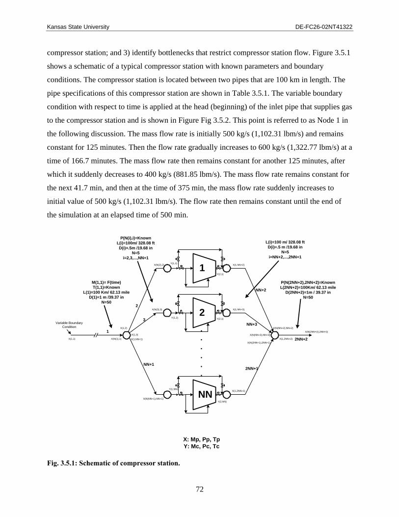
Kansas State University DE-FC26-02NT41322
72
compressor station; and 3) identify bottlenecks that restrict compressor station flow. Figure 3.5.1
shows a schematic of a typical compressor station with known parameters and boundary
conditions. The compressor station is located between two pipes that are 100 km in length. The
pipe specifications of this compressor station are shown in Table 3.5.1. The variable boundary
condition with respect to time is applied at the head (beginning) of the inlet pipe that supplies gas
to the compressor station and is shown in Figure Fig 3.5.2. This point is referred to as Node 1 in
the following discussion. The mass flow rate is initially 500 kg/s (1,102.31 lbm/s) and remains
constant for 125 minutes. Then the flow rate gradually increases to 600 kg/s (1,322.77 lbm/s) at a
time of 166.7 minutes. The mass flow rate then remains constant for another 125 minutes, after
which it suddenly decreases to 400 kg/s (881.85 lbm/s). The mass flow rate remains constant for
the next 41.7 min, and then at the time of 375 min, the mass flow rate suddenly increases to
initial value of 500 kg/s (1,102.31 lbm/s). The flow rate then remains constant until the end of
the simulation at an elapsed time of 500 min.
1
.
.
.
.
.
.
X(1,1) X(N(1),1)
X(1,2)
X(1,3)
X(1,NN+1)
X(N(2),2)
X(N(NN+1),NN+1)
X(1,NN+2)
X(1,2NN+1)
X(N(NN+2),NN+2)
X(N(NN+3),NN+3)
X(N(2NN+1),2NN+1)X(1,2NN+2)
X(N(2NN+2),2NN+2)
Y(1,1)
Y(2,1)
Y(1,NN)
X: Mp, Pp, TpY: Mc, Pc, Tc
1
2
3
NN+1
NN+2
NN+3
2NN+1
2NN+2
2Y(2,1)
NNY(2,NN)
X(N(3),3)
Y(1,2)
X(1,NN+3)
M(1,1)= F(time)T(1,1)=Known
L(1)=100 Km/ 62.13 mileD(1)=1 m /39.37 in
N=50
P(N(i),i)=KnownL(i)=100m/ 328.08 ftD(i)=.5m /19.68 in
N=5i=2,3,...,NN+1
L(i)=100 m/ 328.08 ftD(i)=.5 m /19.68 in
N=5i=NN+2,...,2NN+1
P(N(2NN+2),2NN+2)=KnownL(2NN+2)=100Km/ 62.13 mile
D(2NN+2)=1m / 39.37 inN=50
Variable BoundaryCondition
Fig. 3.5.1: Schematic of compressor station.

Kansas State University DE-FC26-02NT41322
73
This simulation used different types of compressors to demonstrate the difference in gas
parameters and performance data. Specifically, two different compressor stations are considered.
One used centrifugal compressors and the other uses reciprocating compressors. The
specifications of the centrifugal and reciprocating compressors are shown in Tables 3.5.2 and
3.5.3, respectively.
Table 3.5.1: Pipe specifications. Pipe Diameter Length Number of
Nodes
Inlet pipe to the compressor station
1.00 m (39.37 in)
100 km(62.13 mi) 50
Outlet pipe from the compressor station
1.00 m (39.37 in)
100 km(62.13 mi) 50
Inlet pipe to each compressor
0.50 m (19.68 in)
100 m(328.08 ft) 5
Outlet pipe from each compressor
0.50 m (19.68 in)
100 m(328.08 ft) 5
600 Kg/s1322.77 lbm/s
500 Kg/s1102.31 lbm/s
400 Kg/s881.85 lbm/s
Time =0 Time =125 min
Time= 166.7 min
Time = 291.7 min
Time =375 min Time =500 min
500 Kg/s1102.31 lbm/s
Fig. 3.5.2: Changing mass flow rate at Node 1 with respect to time.

Kansas State University DE-FC26-02NT41322
74
The compressor station includes nine identical compressors, all of which operate at the initial
condition of 500 kg/s of natural gas flow through the station (Fig. 3.5.2). As will be shown in the
following section, the control scheme shuts down and starts compressors to match the demand
conditions while maintaining the compressor operating parameters within the specific limits.
Subtask 5.2: Demonstrate VPST with the Base Pipeline System
In order to prove the usability of VPST, the model was tested over a series of cases determined
from Subtask 5.1, as well as on larger scale examples. These cases demonstrate the VPST
capabilities, and the types of results that can be obtained.
Example 1 Base System: Some results for the virtual compressor station described in Subtask
5.1 are shown in Figures 3.5.3 through 3.5.15. Figure 3.5.3 shows the change in mass flow rate
with respect to time for the inlet pipe to the compressor station when different types of
compressors are used. When the inlet pipe inlet mass flow rate is constant at 500 kg/s (1102.31
lbm/s), the flow rate in the pipe gradually increases to the inlet value.
Figure 3.5.3 shows the change in mass flow rate for the inlet pipe from the compressor station.
This variation is similar to that shown in Figure 3.5.4, which is the change in mass flow rate for
the outlet pipe.
Table 3.5.2: Centrifugal compressor specifications. b1 b2 b3 b4 b5 b6
Compressor Map Coefficients
0.3542x10⁻⁴ 0.1013x10⁻² -0.4768x10⁻² 17.269 916.64 3350.8
Table 3.5.3: Reciprocating compressor specifications.
Speed Stroke/Bore Suction/Discharge Pressure Loss
Rod Diameter Clearance Cylinders
300 rpm 14/12.5 in (355.6/317.5 mm) 5% / 5% 3 in
(76.2 mm) 0.1 - 1.6 8

Kansas State University DE-FC26-02NT41322
75
Figure 3.5.5 shows the compressor station fuel consumption as a function of each compressor
type. The mass fuel consumption is almost the same and is about 0.2% of the total mass flow rate
entering the compressor station (note that this percentage is for only one compressor station).
The jumps that are shown in this figure are because of starting and shutting down of
reciprocating compressors.
Time (min)
Mas
sFl
owR
ate
(Dim
ensi
onle
ss)
0 100 200 300 400 500300
400
500
600
700
Node 50
Node 50
Node 50
Node 1
Centrifugal compressor
x 1 kg/sx 2.20462 lbm/s
Time (min)
Mas
sFl
owR
ate
(Dim
ensi
onle
ss)
0 100 200 300 400 500300
400
500
600
700
Node 50
Node 50
Node 1
Node 1
Reciprocating compressor
x 1 kg/sx 2.20462 lbm/s
Fig. 3.5.3: Mass flow rate at the inlet pipe for different types of compressors.
Time (min)
Mas
sFl
owR
ate
(Dim
ensi
onle
ss)
0 100 200 300 400 500300
400
500
600
700
Node 50 Node 50
Node 1
Centrifugal compressor
x 1 kg/sx 2.20462 lbm/s
Time (min)
Mas
sFl
owR
ate
(Dim
ensi
onle
ss)
0 100 200 300 400 500300
400
500
600
700
Node 50
Node 50
Node 1
Node 1
Reciprocating compressor
x 1 kg/sx 2.20462 lbm/s
Fig. 3.5.4: Mass flow rate at the outlet pipe for different types of compressors.

Kansas State University DE-FC26-02NT41322
76
Figures 3.5.6 and 3.5.7 illustrate the pressure distribution within the inlet pipe and the outlet
pipe, respectively. The pressure distribution for each node is different with respect to time due to
the compressibility effects. The pressure distribution is the same for each type of compressor and
is not impacted by changing the number of compressors. Consequently, the type of compressor
and the number of compressors does not have any effect on the up and down stream of
compressor station. This is because, in this simulation, the mass flow rate at the inlet to the pipe
at node 1 is precisely controlled.
Time (min)
Fuel
Con
sum
ptio
n(D
imen
sion
less
)
100 200 300 400 5000
0.2
0.4
0.6
0.8
1
1.2
1.4
1.6Centrifugal CompressorReciprocating Compressor
x 1 kg/sx 2.20462 lbm/s
Time (min)
Fuel
Con
sum
ptio
n(D
imen
sion
less
)
300 350 400
0.6
0.8
Fig. 3.5.5: Fuel consumption for different type of compressors.
Time (min)
Pre
ssur
e(D
imen
sion
less
)
0 100 200 300 400 5004
4.5
5
5.5
6
Node 50
Node 1
Centrifugal compressor
x 1 Mpax 145.0377 Psi
Time (min)
Pre
ssur
e(D
imen
sion
less
)
0 100 200 300 400 5004
4.5
5
5.5
6
Node 1
Node 50
Reciprocating compressor
x 1 Mpax 145.0377 Psi
Fig. 3.5.6: Pressure distribution within the inlet pipe for different types of compressors.

Kansas State University DE-FC26-02NT41322
77
The same type of information is available for the temperature distribution and compressibility
factor distribution for the inlet and outlet pipes. Figures 3.5.8 through 3.5.11 show these
conditions for the temperature and compressibility factor distributions.
Figure 3.5.12 shows the change of power with respect to time for different compressor types. For
this simulation, the centrifugal compressors require more power than the station using
reciprocating compressors. The value of power for reciprocating compressor depends with some
parameter such as valve loss horsepower, which is different for each compressor. Consequently,
this is not a general statement, but can only be stated for this particular case.
Time (min)
Pre
ssur
e(D
imen
sion
less
)
0 100 200 300 400 5004
4.5
5
5.5
6
Node 1
Node 50
Centrifugal compressor
x 1 Mpax 145.0377 Psi
Time (min)
Pre
ssur
e(D
imen
sion
less
)
0 100 200 300 400 5004
4.5
5
5.5
6
Node 1
Node 50
Reciprocating compressor
x 1 Mpax 145.0377 Psi
Fig. 3.5.7: Pressure distribution within the outlet pipe for different types of compressors.
Time (min)
Tem
pera
ture
(Dim
ensi
onle
ss)
0 100 200 300 400 500290
300
310
320
330
340Node 1
Node 3
Node 5
Node 10Node 15
Node 30,40,50
Centrifugal compressor
x 1 Kx 1.8 oR
Time (min)
Tem
pera
ture
(Dim
ensi
onle
ss)
0 100 200 300 400 500290
300
310
320
330
340Node 1
Node 3
Node 5
Node 10Node 15
Node 30, 40, 50
Reciprocating compressor
x 1 Kx 1.8 oR
Fig. 3.5.8: Temperature distribution within the inlet pipe for different types of compressors.

Kansas State University DE-FC26-02NT41322
78
Time (min)
Tem
pera
ture
(Dim
ensi
onle
ss)
0 100 200 300 400 500290
300
310
320
330
340
Node 1
Node 3
Node 5
Node 10
Node 15Node 20,30,40,50
Centrifugal compressor
x 1 Kx 1.8 oR
Time (min)
Tem
pera
ture
(Dim
ensi
onle
ss)
0 100 200 300 400 500290
300
310
320
330
Node 1
Node 3
Node 5
Node 10Node 15
Node 20, 30,40,50
Reciprocating compressor
x 1 Kx 1.8 oR
Fig. 3.5.9: Temperature distribution within the outlet pipe for different types of compressors.
Time (min)
Com
pres
sibi
lity
Fact
or(Z
)
0 100 200 300 400 5000.76
0.78
0.8
0.82
0.84
0.86
0.88
0.9
0.92
0.94Node 1Node 5Node 10Node 20Node 30Node 40Node 50
Node 1
Node 50
Centrifugal compressor
Time (min)
Com
pres
sibi
lity
Fact
or(Z
)
0 100 200 300 400 5000.78
0.8
0.82
0.84
0.86
0.88
0.9
0.92
0.94Node 1Node 5Node 10Node 20Node 30Node 40Node 50
Node 1
Node 50
Reciprocating compressor
Fig. 3.5.10: Compressibility factor within the inlet pipe for different types of compressors.

Kansas State University DE-FC26-02NT41322
79
At 125 minutes, the mass flow rate at Node 1 starts to gradually increase to 600 kg/s (1,322.77
lbm/s). Comparing reciprocating compressors with that of centrifugal compressors shows that
each exhibits different characteristics, such as mass flow rate and pressure distributions because
each compressor has a different control limit. For example, the limit control for a centrifugal
compressor is speed, but for the reciprocating compressor the control limit is via cylinder pocket
clearance. When the control scheme calls for increased mass flow rate, the centrifugal
compressor speed gradually increases as shown in Figure 3.5.13, and the pocket clearance
Time (min)0 100 200 300 400 5000
5000
10000
15000
20000
25000
30000
35000 Power of compressor 1Power of compressor station
x 1 KWx 1.341 HP
Centrifugal Compressor
Power
Time (min)0 100 200 300 400 500
5000
10000
15000
20000
25000
30000
35000 Power of compressor 1Power of compressor station
x 1 KWx 1.341 HP
Reciprocating Compressor
Power
Fig. 3.5.12: Change of power with respect to time for different types of compressors..
Time (min)
Com
pres
sibi
lity
Fact
or(Z
)
0 100 200 300 400 5000.76
0.78
0.8
0.82
0.84
0.86
0.88
0.9
0.92Node 1Node 5Node 10Node 20Node 30Node 40Node 50
Node 1Node 50
Centrifugal compressor
Time (min)
Com
pres
sibi
lity
Fact
or(Z
)
0 100 200 300 400 5000.76
0.78
0.8
0.82
0.84
0.86
0.88
0.9
0.92Node 1Node 5Node 10Node 20Node 30Node 40Node 50
Node 50Node 1
Reciprocating compressor
Fig. 3.5.11: Compressibility factor within the outlet pipe for different types of compressors.

Kansas State University DE-FC26-02NT41322
80
decreases in the reciprocating compressors. Fortunately, speed does not reach the upper or lower
limit in the centrifugal compressor.
After 292 minutes, the mass flow rate requirement is suddenly decreased from 600 kg/s (1322.77
lbm/s) to 400 kg/s (881.85 lbm/s). The centrifugal compressors decrease in speed and the pocket
clearance of the reciprocating compressors increase. However, because of the clearance
limitation in the reciprocating compressors, these compressors are not able to adjust to the
sudden decrease in mass flow rate through pocket clearance alone. Instead, three of the
compressors in this compressor station are shut down as show in Figure 3.5.14.
Figure 3.5.15 shows changing isentropic efficiency with respect to time and compressor map for
centrifugal compressor. The variation in this figure depends on the changing mass flow rate and
compressor speed.
Time (min)0 100 200 300 400 5009000
10500
12000
13500
15000
Speed (rpm)
Upper limit
Lower limit
Time (min)0 100 200 300 400 5000
0.20.40.60.8
11.21.41.61.8
2
Upper limit
Lower limit
Clearance
Fig. 3.5.13: Change in speed of centrifugal compressor and change in clearance for a reciprocating compressor with respect to compressor map.

Kansas State University DE-FC26-02NT41322
81
Example 2 Ten Compressor Stations Each with Three Compression Units: This example
demonstrates the applicability of the VPST for a relatively large pipeline section. The pipeline
considered has 10 compressor stations, and within each compressor there are 3 centrifugal
compressors driven by gas turbines. All the compression units are identical. Figure 3.5.16 shows
the schematic of such a network. All compressor stations are connected using pipes that are 100
Time (min)
Num
bero
fCom
pres
sors
0 100 200 300 400 5005
6
7
8
9
10 Using reciprocating compressorUsing centrifugal compressor
Fig. 3.5.14: Change in the number of branches with respect to time for different types of compressors.
Time (min)
Isen
tropi
cef
ficie
ncy
(%)
0 100 200 300 400 50060
65
70
75
Frame 002 24 Jul 2003 No Data Set
Qac (Dimensionless)
Hea
d(D
imen
sion
less
)
0 0.2 0.4 0.6 0.8 1 1.2 1.4 1.60
10
20
30
40
50
60
70
N=10000 (rpm)
11000
12000
13000
14000
15000
15700
x 1 kj/kgx 334.553 ft.lbf/lbm
x 1 m3/sx 2118.88 cfm
Fig. 3.5.15: Isentropic efficiency plot and compressor map for a centrifugal compressor.

Kansas State University DE-FC26-02NT41322
82
km in length. In each compressor station the design is same as the one shown in Figure 3.5.1
with NN equal to 3. The specifications of all the pipes are provided in Table 3.5.4. All pipes are
assumed to be horizontal, i.e., the angle of inclination of all the pipes is 0.0 radians. The
specifications of the compression unit are specified in Tables 3.5.5 through 3.5.8.
Fig. 3.5.16: Schematic of the 10-station network.
Table 3.5.4: Pipe specifications. Pipe Diameter Length Number of
Nodes Inlet pipe to the compressor station
0.45m (17.72in)
100 km(62.13 mile)
50
Outlet pipe from the compressor station
0.45m (17.72in)
100 km(62.13 mile)
50
Inlet pipe to each compression unit
0.25m (9.84in)
100 m(328.08ft)
5
Outlet pipe from each compression unit
0.25m (9.84in)
100m(328.08ft)
5
Table 3.5.5: Centrifugal compressor specifications.
b1 b2 b3 b4 b5 b6
Compressor Map Coefficients
0.3542x10⁻⁴ 0.1013x10⁻² -0.4768x10⁻² 17.269 916.64 3,350.8

Kansas State University DE-FC26-02NT41322
83
The natural gas flowing through the system is a mixture of methane, ethane and propane in the
ratio of 0.7:0.25:0.05, respectively. The gas parameters are specified in Table 3.5.9.
Figure 3.5.16 also shows the boundary conditions used for the simulation. The boundary
conditions used are constant throughout the simulation. The pressure and temperature at the head
node of the pipe leading to the first compressor station and the pressure at the end node of the
pipe leading out of the last compressor station are treated as boundary conditions. The boundary
condition information is provided in Table 3.5.10. By changing the boundary conditions the
dynamic behavior of any compressor station in the network can be studied. As the network is
large, the time step for the simulation is taken as 2,000 seconds.
Table 3.5.6: Lower and higher gas turbine map coefficients. A1
L A2L A3
L A4L A5
L A6L
Lower Gas Turbine Map Coefficients
0.002085
0.0011308
9
-7.358E-7
22126.6
-35.7514
0.0246
A1H A2
H A3H A4
H A5H A6
H
Higher Gas Turbine Map Coefficients
0.004036
0.0013639
-9.5537E-7
21834.2
-38.8951
0.0293973
Table 3.5.7: Adjustment coefficients for lower and higher gas turbine map equations.
b1L b2
L b1H b2
H Gas Turbine Map Coefficients
2.0 3.5 1.0 -0.5
Table 3.5.8 :Other gas turbine parameters. Heat Rate ηmech TB TEN 4.0 kJ/kg 0.98 260.9278 K 298.15 K
Table 3.5.9: Natural gas properties. Mole
Fraction Molecular
Weight Specific Heat at
50
Specific Heat at
300
Critical Pressure
Critical Temp
Density Lower Heating Value
Methane 0.70 16.042 8.414E3 10.01E3 667.8 343.04 0.7168 55,601
Ethane 0.25 30.068 12.17E3 16.34E3 707.8 549.76 1.356 51,958
Propane 0.05 44.097 16.88E3 23.56E3 616.3 665.68 2.019 50,409

Kansas State University DE-FC26-02NT41322
84
As mentioned in earlier sections, the dynamic simulation of the compressor station network
involves: 1) nonlinear partial differential equations that describe the pipe flow; and 2) nonlinear
algebraic equations that describe the compression units and junctions. The pressure, temperature
and mass flow rate variations over the line pipe were explained in earlier sections. The main aim
is to study the behavior of the compression unit parameters with respect to time for different
compressor stations. For this, one compression unit from each compressor station is selected and
its parameters are studied over a time period. Figures 3.5.17 through 3.5.22 show the variations
of speed, power, efficiency, fuel consumption, head, discharge pressure, discharge temperature
and discharge mass flow rate for a compression unit from each of the 10 compressor stations
with respect to time. All the parameters are across a selected single compression unit.
For all the parameters, the compression unit in the compressor station reaches steady state. As
the unit gets further downstream, more time is required to reach steady state. Thus, the first
compressor station reaches steady state condition first and the tenth compressor station reaches
steady state last.
The mass flow rate decreases as it passes each compressor station as some of the fuel is
consumed by the gas turbine. The power and speed needed for the compression unit decreases as
we go from one compressor station to the next. This can be seen in Fig 3.5.17. The compression
unit in station 1 needs more power and works at a higher speed, than the one in station 10,
because the mass flow is more.
Table 3.5.10: Boundary conditions for 10 compressor stations each with 3 compression units.
Component ID Node # Parameter Value Pipe ‘PA’ 1 Pressure 6.184E6 Pa
Pipe ‘PA’ 1 Temperature 333.15 K
Pipe ‘PBS’ 2 Pressure 5.11E6 Pa

Kansas State University DE-FC26-02NT41322
85
The head of the compressor depends on its suction and discharge pressure. The difference
between the suction and discharge pressures for the compressors in the first station should be
more than in the last station. Thus, the head of the compression unit decreases as the compressor
station number increases as seen in Figures 3.5.18 and 3.5.19.
Fuel consumption depends on the head of the compression unit. Figure 3.5.20 shows that though
the fuel consumption increases along the compressor stations the difference is not great. As the
compression unit in the first station works with a higher difference between the suction and
discharge pressures, the discharge temperature is higher as compared to the last station, as shown
in Figure 3.5.21.
Fig 3.5.17 Comparisons of speed and power at each compressor station over time.
Fig. 3.5.18: Comparisons of suction and discharge pressures at each compressor station over time.

Kansas State University DE-FC26-02NT41322
86
The suction mass flow rate for a compression unit is greater than the discharge mass flow rate as
a small percent of the gas is used by the gas turbine to drive the compressor. This can be seen in
Fig 3.5.22.
Fig. 3.5.19: Comparison of head at each compressor station over time.
Fig. 3.5.20: Comparison of fuel consumption at each compressor station over time.
Fig. 3.5.21: Comparison of suction and discharge temperatures at each compressor station over time.

Kansas State University DE-FC26-02NT41322
87
Example 3 Ten Compression Stations Each with Five Compression Units: In this example
the pipeline has 10 compressor stations, and within each compressor station there are 5
compression units consisting of centrifugal compressors driven by gas turbines. All the
compression units are identical. The schematic of the network is the same as that in Fig 3.5.16.
All compressor stations are connected using long pipes that are 100 km in length. In each
compressor station the design is the same as the one shown in Figure 3.5.1 with NN equal to 5.
The specifications of all the pipes are the same as in Table 3.5.4. The angle of inclination of all
the pipes is 0.0 radians. The specifications of the compression units are the same as in Tables
3.5.5 to 3.5.7. The natural gas flowing is a mixture of methane, ethane and propane in the ratio
0.7:0.25:0.05, respectively. The natural gas parameters are same as in Table 3.5.8.
Figure 3.5.16 also shows the boundary conditions used for the simulation. The boundary
conditions used are constant throughout the simulation. The boundary condition information is
provided in Table 3.5.10. By changing the boundary conditions the dynamic behavior of any
compressor station in the network can be studied. As the network is large, the time step for the
simulation is taken as 2,000 seconds.
Fig. 3.5.22: Comparison of suction and discharge mass flow rates at each compressor station over time.

Kansas State University DE-FC26-02NT41322
88
The pressure, temperature and mass flow rate variations over the line pipe are as explained in the
previous example. The variation of the compression unit parameters with respect to time for
different compressor stations needs to be observed. For this, one compression unit from each
compressor station is selected and its parameters are studied over a time period. Figures 3.5.23
through 3.5.28 show the variations of speed, power, fuel consumption, head, discharge pressure,
discharge temperature and discharge mass flow rate for a compression unit from each of the 10
compressor stations with respect to time. All the parameters are for a selected single compression
unit in the compressor station.
The mass flow rate decreases as it passes each compressor station as some of the fuel is
consumed by the gas turbine. Thus the power needed for the compression unit decreases from
one compressor station to the next, and hence the speed at which it runs decreases. This can be
seen in Figure 3.5.23. The compression unit in the first station needs more power and runs faster
than the last station, as the mass flow is more.
The head of the compressor depends on its suction and discharge pressure. The difference
between the suction and discharge pressures for the compressors in the first station should be
more than for the same in the last station. Thus, the head of the compression unit decreases as the
compressor station number increases. Figures 3.5.24 and 3.5.25 show this trend.
Fig. 3.5.23: Comparison of speed and power at each compressor station over time.

Kansas State University DE-FC26-02NT41322
89
As the compression unit in the first station works
with a higher difference between the suction and
discharge pressures, the temperature at discharge
is higher in comparison to the same in the last
station, as shown in Figure 3.5.26.
Fuel consumption depends on the head of the
compression unit. Figure 3.5.27 shows that though
the fuel consumption changes along the
compressor stations, the difference is small.
Fig. 3.5.24: Comparison of suction and discharge pressure at each compressor station over time.
Fig. 3.5.25: Comparison of head at each compressor station over time.
Fig. 3.5.26: Comparison of suction and discharge temperature at each compressor station over time.

Kansas State University DE-FC26-02NT41322
90
The suction mass flow rate for a compression
unit is greater than the discharge mass flow
rate as a small percent of the gas is used by
the gas turbine to drive the compressor. This
can be seen in Figure 3.5.28.
Fig.3.5.27: Comparison of fuel consumption at each compressor station over time.
Fig. 3.5.28: Comparison of suction and discharge mass flow rates at each compressor station over time.

Kansas State University DE-FC26-02NT41322
91
4.0 CONCLUSIONS
This study uses a fully implicit finite difference method to analyze transient, non-isothermal
compressible gas flow through a gas pipeline system. The inertia term of the momentum
equation is included in the analysis. The numerical results show that:
• Optimization
Operational optimization using rigorous mathematical techniques is a viable tool for
enhancing the efficiency of pipeline operations. Currently available commercial packages
do not provide the capability for fully automated optimization of operational parameters;
rather, these packages provide computational support for human decision making. In
other words, the current generation of software in this area allows a human operator to
simulate pipe flow in a network without detailed modeling of equipment such as
compressors and drivers. Any decisions on how to optimize the operation of equipment
must be made by the human operator based on simplified simulation of a few scenarios.
Thus, the solutions are generally not truly optimal, and require considerable user
involvement. This work advances the current state of pipeline simulations by using
detailed equipment modeling and rigorous mathematical optimization that will
automatically generate truly optimal solutions with practically no user involvement. This
represents a significant advancement in the state-of-the-art in this field.
• Solution Method
The fully implicit method has advantages, such as the guaranteed stability for large time
step, which is very useful for simulating long-term transients in natural gas pipelines. The
inertia term plays an important role in the gas flow analysis and cannot be neglected in
the calculation. The effect of treating the gas in a non-isothermal manner is very
necessary for pipeline flow calculation accuracies, and is extremely necessary for rapid
transient processes. By using a computer simulation, the dynamic response of the
compressor can be determined by changing boundary condition with respect to time. The
current simulation lays a foundation on which to build a more detailed compressor station
model with equipment such as scrubbers, coolers, etc. The penetrations of sudden

Kansas State University DE-FC26-02NT41322
92
property changes along long length pipes are very small. The model was validated by
comparing simulated results with those of others. The solution method was used to solve
a large scale problem that included ten compressor stations, each with five compression
units.
• Implementation
The implementation of the simulation methods included the development of a graphical
user interface called the Pipeline Editor. This editor is a feature-rich graphical user
interface designed to provide pipeline designers with a graphical view of a pipeline
systems and simulation data. The Pipeline Editor can be used to graphically build the
pipeline system, manipulate an already built graph, simulate the model using parallel or
sequential simulators, and display the results of such simulation graphically. The Pipeline
Editor was developed using the Jgraph and Swing packages. The editor is an easy to use
application that can be started from any computer using an Internet browser. Once started
the Pipeline Editor connects to the Optimizer and the Sequential and Parallel Simulators.
The application requires Java Web Start 1.2 and for execution.

Kansas State University DE-FC26-02NT41322
93
5.0 REFERENCES
Ariel Corporation, 2001, “Ariel Application Method,” http://12.2.241.6:9980/ariel/ext_data/application_manual/arieldb.htm.Beam, R.M., and Warming, R.F., 1975, “An Implicit Finite-Difference Algorithm for Hyperbolic Systems in Conservation-Law Form”, Journal of Computational Physics, No.22, pp. 87-110.
Berard, G.P., and Eliason, B.G., 1978, “An Improved Gas Transmission System Simulator”, Society of Petroleum Engineers Journal, Dec., pp. 389-398.
Botros, K.K., 1990, “Thermodynamic Aspects of Gas Recycling During Compressor Surge Control”, ASME Proceeding Pipeline Engineering Symposium, New Orleans, Louisiana, pp. 57-65.
Botros, K.K., 1994, “Transient Phenomena in Compressor Stations during Surge”, Journal of Engineering for Gas Turbines and Power, Vol. 116, Jan., pp.133-142.
Botros, K.K., Campbell, P.J., and Mah, D.B., 1989, “Dynamic Simulation of Compressor Station Installations Including Control Systems”, 21st Annual Meeting Pipeline Simulation Interest Group (PSIG), Oct. 19-20, El Paso, Texas.
Botros, K.K., Campbell, P.J., and Mah, D.B., 1991, “Dynamic Simulation of Compressor Station Operation Including Centrifugal Compressor and Gas Turbine”, Transactions of the ASME, Vol. 113, Apr., pp. 300-311.
Bryant, M., 1997, “Complex Compressor Station Modeling”, 29th Annual Meeting Pipeline Simulation Interest Group (PSIG), Oct. 15-17, Tucson, Arizona.
Cameron, I., 1999, “Using An Excel-Based Model for Steady State and Transient Simulation”, 31st Annual Meeting Pipeline Simulation Interest Group (PSIG), Oct. 20-22, St. Louis, Missouri.
Carter, R.G., 1996, “Compressor Station Optimization: Computational Accuracy and Speed”, 28th Annual Meeting Pipeline Simulation Interest Group (PSIG), Oct. 23-25, San Francisco, California.
Chang, S., 2001, “A Program Development for Unsteady Gas Flow Analysis in Complex Pipe Networks”, 33rd Annual Meeting Pipeline Simulation Interest Group (PSIG), Oct. 17-19, Salt Lake City, Utah.
Chapman, K.S., Abbaspour, M. and Keshavarz, A., 2003, “Development of a Virtual Pipeline System Testbed Using Non-Isothermal Transient Simulation”, Gas Machinery Conference, Oct. 6-8, Salt Lake City, UT.
Chapman, K.S., and Keshavarz-Valian, A., 2003, “Development of Turbocharger-Reciprocating Engine Simulation (T-RECS),” Gas Research Institute, GRI-03/0005.

Kansas State University DE-FC26-02NT41322
94
Costa, L.H, de Medeiros, J.L., and Pessoa, F.L.P, 1998, “Steady State Modeling and Simulation of Pipeline Networks for Compressible Fluids”, Brazilian Journal of Chemical Engineering, Vol.15, No.4.
Deen, J.K., and Reintsema, S.R, 1983, “Modeling of High-Pressure Gas Transmission Lines”, Appl. Math. Modeling, Vol.7, Aug. pp. 268-273.
Doonan, A.F., Fletcher, I. Cox, C.S., and Arden W.J.B., 1998, “Evaluation of A Remote Boundary Pressure Control Strategy Using SIMULINKTM “, Proceeding from UKACC International Conference on Control’ 98, Sep. 1-4, No.455, pp.129-134.
Dranchuck, P.M., Purvis, R.A., and Robinson, D.B., 1974, “Computer Calculations of Natural Gas Compressibility Factors Using the Standing and Katz Correlation”, Institute of Petroleum Technical Series, No. IP 74-008, pp.1-13.
Dupont, T., and Rachford, H.H., 1980, “The Effect of Thermal Changes Induced by Transients in Gas Flow”, 12th Annual Meeting Pipeline Simulation Interest Group (PSIG), Oct. 16-17, Savannah, Georgia.
Fauer, D., 2002, “The Making of a Useful Pipeline Simulation Model”, 34th Annual Meeting Pipeline Simulation Interest Group (PSIG), Oct. 23-25, Portland, Oregon.
Greyvenstein, G.P., and Laurie, D.P., 1994, “A Segregated CFD Approach to Pipe Network Analysis”, International Journal for Numerical Methods in Engineering, Vol. 37, pp. 3685-3705.
Hartwick, W., 1968, “Efficiency Characteristics of Reciprocating Compressors,” American Society of Mechanical Engineers. Diesel and Gas Engine Power Division, Dec. 1-5.
Hartwick, W., 1974, “Power Requirements and Associated Effects of Reciprocating Compressor Cylinder Ends Deactivated by Internal Bypassing,” American Society of Mechanical Engineers. Diesel and Gas Engine Power Division, Dec. 17.
Hati, A., Verma, N., and Chhabra, R., 2001, “Transient Analysis of Gas Flow in a Straight Pipe”, Canadian Journal of Chemical Engineering, Vol. 79, No. 1, Feb. pp. 18-27.
Heath, M.J., and Blunt, J.C., 1969, “Dynamic Simulation Applied to the Design and Control of a Pipeline Network”, J. Inst. Gas. Eng., Vol. 9, No. 4, pp. 261-279.
Hoeven, T.V., and Gasunie, N.V.N., 1992, “Some Mathematical Aspects of Gas Network Simulation”, 24th Annual Meeting Pipeline Simulation Interest Group (PSIG), Oct. 22-23, Corpus Christi, Texas.
Ibraheem, S.O., and Adewumi, M.A., 1996, “Higher-Resolution Numerical Solution for 2-D Transient Natural Gas Pipeline Flows”, Society of Petroleum Engineers, SPE 35626, pp. 473-482.

Kansas State University DE-FC26-02NT41322
95
Issa, R.I., and Spalding, D.B., 1972, “Unsteady One-Dimensional Compressible Frictional Flow with Heat Transfer”, Journal Mechanical Engineering Science, Vol. 14, No.6, pp. 365-369.
Jenicek, T., and Kralik, J., 1995,” Optimized Control of Generalized Compressor Station”, 27th Annual Meeting Pipeline Simulation Interest Group (PSIG), Oct. 18-20, Albuquerque, New Mexico
Kiuchi, T., 1994, “An Implicit Method for Transient Gas Flow in Pipe Networks”, Int. J. Heat and Fluid Flow, Vol. 15, No. 5, pp. 378-383.
Letnowski, F.W., 1993, “Compressor Station Modeling in Networks”, 25th Annual Meeting Pipeline Simulation Interest Group (PSIG), Oct. 14-15, Pittsburgh, Pennsylvania.
Lewandowski, A., 1994, “Object-oriented Modeling of the Natural Gas Pipeline Network”, 26th Annual Meeting Pipeline Simulation Interest Group (PSIG), Oct. 13-14, San Diego, California.
Ludwig, E.E., 1983, “Applied Process Design for Chemical and Petrochemical Plants”, Gulf Publishing Company, Houston, Texas.
Luongo, C.A., 1986, “An Efficient Program for Transient Flow Simulation in Natural Gas Pipelines”, 15th Annual Meeting Pipeline Simulation Interest Group (PSIG), Oct. 30-31, New Orleans, Louisiana.
Maddox, R.N., and Zhou, P., 1983, “Use of Steady –State Equations for Transient Flow Calculations”, 15th Annual Meeting Pipeline Simulation Interest Group (PSIG), Oct. 27-28, Detroit, Michigan .
Martinz-Romero, N., Osorio-Peralta, O., and Santamaria-Vite, I., 2002, “Natural Gas Network Optimization and Sensibility Analysis”, Proceedings of the SPE International Petroleum Conference and Exhibition of Mexico, Feb. 10-12, pp. 357-370.
Mathews, H., 2000, “Compressor Performance Analysis,” Proceedings of the 2000 Gas Machinery Conference, Oct. 4, Colorado Springs, Colorado.
McConnell, P., Smith, C., Maguire, P., and Turner, W.J., 1992, “Real-Time and Prediction Model of the Moomba-Sydney-Newcastle Natural Gas Pipeline”, 24th Annual Meeting Pipeline Simulation Interest Group (PSIG), Oct. 22-23, Corpus Christi, Texas.
Metcalf, J.R., 2000, “Effects of Compressor Valves on Reciprocating Compressor Performance,” Proceedings of the 2000 Gas Machinery Conference, Oct. 4, Colorado Springs, Colorado.
Modisette, J., 2002, “Pipeline Thermal Model”, 34th Annual Meeting Pipeline Simulation Interest Group (PSIG), Oct. 23-25, Portland, Oregon

Kansas State University DE-FC26-02NT41322
96
Mohitpour, M., Thompson, W., and Asante, B., 1996, “Importance of Dynamic Simulation on the Design and Optimization of Pipeline Transmission Systems”, Proceedings of the International Pipeline Conference, American Society of Mechanical Engineers, Vol.2, pp. 1183-1188.
Murphy, H.G., 1989, “Compressor Performance Modeling to Improve Efficiency and the Quality of Optimization Decisions,” 21st Annual Meeting Pipeline Simulation Interest Group (PSIG), Oct. 19-20, El Paso, Texas.
Odom, F.M., 1990, “Tutorial on Modeling of Gas Turbine Driven Centrifugal Compressors”, 22nd Annual Meeting Pipeline Simulation Interest Group (PSIG), Oct. 18-19, Baltimore, Maryland.
Osiadacz, A.J., 1987, Simulation and Analysis of Gas Networks, Gulf Publishing Company, Houston, Texas.
Osiadacz, A.J., 1994, “Dynamic Optimization of High Pressure Gas Networks Using Hierarchical Systems Theory”, 26th Annual Meeting Pipeline Simulation Interest Group (PSIG), Oct. 13-14, San Diego, California.
Osiadacz, A.J., 1996, “Deferent Transient Models- Limitations, Advantages and Disadvantages”, 28th Annual Meeting Pipeline Simulation Interest Group (PSIG), Oct. 23-25, San Francisco, California.
Osiadacz, A.J., and Bell, D.J., 1995, “Dynamic Simulation of Gas Networks by Decomposition and Coordination”, Mathematical Engineering in Industry,. Vol. 5, No. 3, pp. 235-254.
Osiadacz, A.J., and Chaczykowski, M., 1998, “Comparison of Isothermal and Non-Isothermal Transient Models”, 30th Annual Meeting Pipeline Simulation Interest Group (PSIG), Oct. 28-30, Denver, Colorado.
Osiadacz, A.J., and Chaczykowski, M., 2001, “Simulation of Non-Isothermal Transient Gas Flow in a Pipeline”, Archives of Thermodynamics, Vol. 22, No. 1-2, pp. 51-70.
Ouyang, L. and Aziz, K., 1996, “Steady-State Gas Flow in Pipes”, Journal of Petroleum Science and Engineering, Vol.14, pp. 137-158.
Patankar, S. V., 1980, Numerical Heat Transfer and Fluid Flow, Hemisphere, Washington.
Phillippi, G, 2002, “Basic Compression Short Course”, Proceedings from the 2002 Gas Machinery Conference, Oct 7-9, Nashville, TN.
Pierson, J. L., and Wilcox, K. D., 1984, “A Computer System for Analysis of Multi-Stage Reciprocating Compressors,” 16th Annual Meeting Pipeline Simulation Interest Group (PSIG), Oct. 18-19, Chattanooga, Tennessee.

Kansas State University DE-FC26-02NT41322
97
Price, G.R, McBrien, R.K., Rizopoulos, S.N., and Golshan, H., 1996, “Evaluating the Effective Friction Factor and Overall Heat Transfer Coefficient During Unsteady Pipeline Operation”, Proceedings of the International Pipeline Conference, American Society of Mechanical Engineers, Vol.2, pp. 1175-1182.
Rachford, H.H., and Dupont, T.A., 1974, “A Fast Highly Accurate Means of modeling Transient Flow in Gas Pipelines by Variational Methods”, Society of Petroleum Engineers Journal, pp. 356-362.
Rhoads, G.A., 1983, “Which Flow Equation - Does it Matter?” 15th Annual Meeting Pipeline Simulation Interest Group (PSIG), Oct. 27-28, Detroit, Michigan.
Rios-Mercado, R.Z., Suming, W., Ridgway, S., and Boyd, A., 2001, “A Reduction Technique for Natural Gas Transmission Network Optimization Problems”, Annals of Operation Research, Vol. 117, pp. 217-234.
Santos, S.P., 1997, “Transient Analysis, A Must in Gas Pipeline Design”, 29th Annual Meeting Pipeline Simulation Interest Group (PSIG), Oct. 15-17, Tucson, Arizona.
Schroeder, D.W., 2001, “A Tutorial on Pipe Flow Equations”, 33rd Annual Meeting Pipeline Simulation Interest Group (PSIG), Oct. 17-19, Salt Lake City, Utah.
Schultz, J.M., 1962, “The Polytropic Analysis of Centrifugal Compressors”, Journal of Engineering for Power, Jan., pp. 69-82.
Shapiro, A.H., 1953, The Dynamics and Thermodynamics of Compressible Fluid Flow, Volume. 1, John Wiley & Sons.
Stanley, R.A., and Bohannan, W.R., 1977, “Dynamic Simulation of Centrifugal Compressor Systems”, Proceedings of the Sixth Turbomachinery Symposium, pp. 123-131.
Stoner, M.A., 1969, “Steady- State Analysis of Gas production Transmission and Distribution Systems”, Society of Petroleum Engineers of AIME, SPE 2554.
Stoner, M.A., 1972, “Sensitivity Analysis Applied to a Steady-State Model of Natural Gas Transportation Systems”, Society of Petroleum Engineers Journal, Apr., pp. 115-125.
Sung, W., Huh, D., Lee, J., and Kwon, O., 1998, “Optimization of Pipeline Networks with a Hybrid MCST-CD Networking Model”, SPE Production & Facilities, August, Vol.13, No..3, pp. 213-219.
Tanaka, T., 1983, “A Computer Simulation of Unsteady-State Gas Flow in Pipeline”, J. Japan Petrol. Inst. No. 26, pp.67-77.
Tao, W.Q., and Ti, H.C., 1998, “Transient Analysis of Gas Pipeline Network”, Chemical Engineering Journal, No. 69, pp.47-52.

Kansas State University DE-FC26-02NT41322
98
Thorley, A.R.D., and Tiley, C.H., 1987, “Unsteady and Transient Flow of Compressible Fluids in Pipelines - A Review of Theoretical and Some Experimental Studies”, Journal of Heat and Fluid Flow, Vol.8, No.1, pp. 3-15.
Tian, S. and Adewumi, M.A., 1994, “Development of Analytical Design Equation for Gas Pipelines”, SPE Production & Facilities, pp. 100-106.
Turner, W.J., and Simonson, M.J., 1984, “A Compressor Station Model for Transient Gas Pipeline Simulation”, 16th Annual Meeting Pipeline Simulation Interest Group (PSIG), Oct. 18-19, Chattanooga, Tennessee.
Turner, W.J., and Simonson, M.J., 1985, “Compressor Station Transient Flow Modeled”, Oil & Gas Journal Technology, May, pp. 79-83.
Wylie, E.B., Stoner, M.A., and Streeter, V.L., 1971, “Network System Transient Calculation by Implicit Methods”, Society of Petroleum Engineers Journal, Dec., pp. 356-362.
Wylie, E.B., Streeter, V.L., and Stiner, M.A., 1974, “Unsteady State Natural-Gas Calculations in Complex Piping Systems”, Society of Petroleum Engineers Journal, Feb., pp. 35-43.
Yow, W., 1971, “Analysis and Control of Transient Flow in Natural Gas Piping Systems”, Ph.D. Thesis, The University of Michigan.
Zemansky, M.W., 1968, Heat and Thermodynamics 5th Edition, McGraw Hill.
Zhou, J. and Adewumi, M.A., 1995, “Simulation of Transient Flow in Natural Gas Pipelines”, 27th Annual Meeting Pipeline Simulation Interest Group (PSIG), Oct. 18-20, Albuquerque, New Mexico.

Kansas State University DE-FC26-02NT41322
99
APPENDIX A: FORMULATION OF GOVERNING PIPELINE SIMULATION EQUATIONS
This appendix includes all the details of the pipeline governing equations. While this level of
detail is beyond the interest level of the typical reader, it was not found in any of the other
literature, including text books. Hence, this information is included in this report to provide the
pipeline simulation professional a concise development of the transient, non-isothermal
compressible flow equations.
A.1 Governing Equations
The non-isothermal flow of natural gas in pipelines is governed by the time-dependent
continuity, momentum, energy equations (Luongo 1986) and equation of state for homogeneous,
geometrically one-dimensional flow. By simultaneously solving these equations, one can obtain
the flow rate as well as the behavior of gas parameters along the pipe network.
A.1.1 Continuity Equation
The mass conservation concept illustrated for the control volume shown in Figure A.1.1 can be
θ
x
dy
y
D
dX
AVρ( )Adx
tρ∂
∂
( )AV AV dxx
ρ ρ∂+∂
Fig. A.1.1: Control volume for the continuity equation.

Kansas State University DE-FC26-02NT41322
100
written as:
( ) ( )Av Av Av dx Adxx t
ρ ρ ρ ρ∂ ∂− − =
∂ ∂ (A.1.1)
Then,
( ) ( ) 0Av dx Adxx tρ ρ∂ ∂
+ =∂ ∂
(A.1.2)
Simplifying, the mass conservation equation reduces to:
( ) 0vt xρ ρ∂ ∂+ =
∂ ∂ (A.1.3)
Where ρ is the density of the fluid ( )3kg
m and v is the velocity of fluid directed along the axis
of the pipe ( )m s .
A.1.2 Momentum Equation
The momentum equation can be written for the control volume shown in Figure A.1.2 using the
θ
θ
x
PA
( )PA PA dxx
+∂∂
dyg Adxdx
ρ
dy
y0 Ddxπτ
D
dX
Fig. A.1.2: Control volume for the momentum equation.

Kansas State University DE-FC26-02NT41322
101
following force component summation:
( ) ( )0dy v vPA PA PA dx Ddx gAdx Adx v
x dx x tπ ρ ρτ∂ ∂ ∂⎛ ⎞ ⎛ ⎞− − − − = +⎜ ⎟ ⎜ ⎟∂ ∂ ∂⎝ ⎠ ⎝ ⎠
(A.1.4)
Reducing and algebraically manipulating the momentum equation results in:
0P dy v vA D gA A vx dx x t
π ρ ρτ∂ ∂ ∂⎛ ⎞ ⎛ ⎞− − − = +⎜ ⎟ ⎜ ⎟∂ ∂ ∂⎝ ⎠ ⎝ ⎠ (A.1.5)
The parameter 0τ is the shear stress between the fluid and the pipe wall and can be obtained by:
0 8f v vρτ = (A.1.6)
The variable f is the Darcy friction factor. The absolute value of v is introduced to maintain the
correct direction for negative velocities. Various researchers have used different relationships to
define the friction factor by specifying a variety of functional relationships for f. Recognizing
that dy Sindx
θ= , the momentum equation is reduced to:
8
f v vP v vA D gASin A vx x t
ρπ ρ θ ρ∂ ∂ ∂⎛ ⎞− − − = +⎜ ⎟∂ ∂ ∂⎝ ⎠
(A.1.7)
and,
8
f v vw D
ρπ= (A.1.8)
Then,
v v P wv gSint x x A
ρ ρ ρ θ∂ ∂ ∂+ + = − −
∂ ∂ ∂ (A.1.9)

Kansas State University DE-FC26-02NT41322
102
A.1.3 Conservation of Energy
The basic form of the conservation of energy equation from the first law of thermodynamics
(Shapiro 1953) is written for the control volume shown in Figure A.1.3 as:
2 2
2 2v v PQ q Adx Adx u gy vA u gy dx
t xρ ρ ρ
ρ⎡ ⎤ ⎡ ⎤⎛ ⎞ ⎛ ⎞∂ ∂
= = + + + + + +⎢ ⎥ ⎢ ⎥⎜ ⎟ ⎜ ⎟∂ ∂⎝ ⎠ ⎝ ⎠⎣ ⎦ ⎣ ⎦ (A.1.10)
where q is the heat addition per unit mass per unit time and u is the internal energy.
Separating the second term results in:
2 2
2 2v vq Adx Adx u gy v u gy
t xρ ρ
⎡ ⎤⎛ ⎞ ⎛ ⎞∂ ∂= + + + + +⎢ ⎥⎜ ⎟ ⎜ ⎟∂ ∂⎝ ⎠ ⎝ ⎠⎣ ⎦
( ) ( )2
2A vAvu gy dx
t xρ ρ⎡ ⎤∂ ∂⎛ ⎞⎛ ⎞
+ + + +⎢ ⎥⎜ ⎟⎜ ⎟ ∂ ∂⎢ ⎥⎝ ⎠⎝ ⎠⎣ ⎦ (A.1.11)
( ) ( )vAP PvA dxx xρ
ρρ ρ
⎡ ⎤∂ ⎛ ⎞∂+ +⎢ ⎥⎜ ⎟∂ ∂ ⎝ ⎠⎣ ⎦
θ
x
dy
y0 Ddxπτ
D
dX
Q
VT
Fig. A.1.3: Control volume for the energy equation.

Kansas State University DE-FC26-02NT41322
103
From the continuity equation the second term will be zero ( ) ( ) 0A vA
t xρ ρ∂ ∂⎛ ⎞
+ =⎜ ⎟∂ ∂⎝ ⎠.
Dividing by Adxρ , the energy equation reduces to:
2 ( )
2D v v P P vAq u gyDt x A xρ ρ
⎛ ⎞ ∂ ∂= + + + +⎜ ⎟ ∂ ∂⎝ ⎠
(A.1.12)
Using the momentum equation and multiplying by v results in:
v P Dv wvv vgSinx Dt A
θρ ρ∂
= − − −∂
(A.1.13)
So from continuity equation it can show that:
( ) D AvAx Dt
ρρ
∂= −
∂ (A.1.14)
Then,
2
22D v Dv wv P Dq u gy v vgSinDt Dt A Dt
ρθρ ρ
⎛ ⎞= + + − − − −⎜ ⎟
⎝ ⎠ (A.1.15)
On the other hand, considering the identity:
( )D y ygy g v gvSinDt t x
θ∂ ∂⎛ ⎞= + =⎜ ⎟∂ ∂⎝ ⎠ (A.1.16)
and,
2
2D v DvvDt Dt
⎛ ⎞=⎜ ⎟
⎝ ⎠ (A.1.17)
results in:

Kansas State University DE-FC26-02NT41322
104
2
Du P D wvqDt Dt A
ρρ ρ
= − − (A.1.18)
So that:
Ph uρ
≡ + (A.1.19)
and then:
Dh Du D PDt Dt Dt ρ
⎛ ⎞= + ⎜ ⎟
⎝ ⎠ (A.1.20)
Finally, this equation can be expanded to:
2
1Dh Du P D DPDt Dt Dt Dt
ρρ ρ
= − + (A.1.21)
and the energy equation reduces to:
1wv Dh DPqA Dt Dtρ ρ
+ = − (A.1.22)
Recognizing that q AρΩ = provides the final form of the conservation of energy equation:
h h P P wvv vt x x x A
ρ ρ∂ ∂ ∂ ∂ Ω++ − − =
∂ ∂ ∂ ∂ (A.1.23)
where h is the specific enthalpy ( )Jkg , Ω is the hHeat flow into the pipe per unit length of
pipe per unit time ( )( . )J
m s , and A is the cCross-sectional area of pipe 2
4Dπ⎛ ⎞
⎜ ⎟⎝ ⎠
( )2m .

Kansas State University DE-FC26-02NT41322
105
A.1.4 Equation of State
An equation of state for a gas relates the variables P , ρ and T . The type of equation, which is
commonly used in gas industry, is:
P ZRTρ= (A.1.24)
where Z is the compressibility factor which is a function of P and T , and R is the specific gas
constant ( )Jkg .
In their current form, equations (A.1.3), (A.1.9) and (A.1.18) are not convenient to solve.
Therefore these equations need to be rewritten in terms of pressure, velocity and temperature as
the dependent variables by using the equation of state. To obtain ρ in terms of P , Z , and
T from the equation of state:
PZRT
ρ = (A.1.25)
Therefore:
( ) ( ) ( ) ( ) ( )ln ln ln ln lnP R T Zρ = − − − (A.1.26)
Differentiating this equation with respect of time:
1 1 1 1 1D DP DR DT DZDt P Dt R Dt T Dt Z Dtρ
ρ= − − − (A.1.27)
The term 1 DRR Dt
is zero, so the compressibility factor is a function of P and T such that:
T P
Z ZdZ dP dTP T∂ ∂⎛ ⎞ ⎛ ⎞= +⎜ ⎟ ⎜ ⎟∂ ∂⎝ ⎠ ⎝ ⎠
(A.1.28)

Kansas State University DE-FC26-02NT41322
106
T P
DZ Z DP Z DTDt P Dt T Dt
∂ ∂⎛ ⎞ ⎛ ⎞= +⎜ ⎟ ⎜ ⎟∂ ∂⎝ ⎠ ⎝ ⎠ (A.1.29)
therefore:
1 1 1 1 1
T P
D Z DP Z DTDt P Z P Dt T Z T Dtρ
ρ⎧ ⎫ ⎧ ⎫∂ ∂⎛ ⎞ ⎛ ⎞= − − +⎨ ⎬ ⎨ ⎬⎜ ⎟ ⎜ ⎟∂ ∂⎝ ⎠ ⎝ ⎠⎩ ⎭ ⎩ ⎭
(A.1.30)
Substituting this into equation (A.1.3):
1 1 1 1 0T P
Z DP Z DT vP Z P Dt T Z T Dt x
⎧ ⎫ ⎧ ⎫∂ ∂ ∂⎛ ⎞ ⎛ ⎞− − + + =⎨ ⎬ ⎨ ⎬⎜ ⎟ ⎜ ⎟∂ ∂ ∂⎝ ⎠ ⎝ ⎠⎩ ⎭ ⎩ ⎭ (A.1.31)
To obtain h in terms of P , Z , and T , Zemansky (1968) described the thermodynamic identity
for enthalpy as:
1P
T dPdh CpdTTρ
ρ ρ⎧ ⎫∂⎛ ⎞= + +⎨ ⎬⎜ ⎟∂⎝ ⎠⎩ ⎭
(A.1.32)
and then:
11P
Dh DT T DPCpDt Dt T Dt
ρρ ρ
⎧ ⎫∂⎛ ⎞= + +⎨ ⎬⎜ ⎟∂⎝ ⎠⎩ ⎭ (A.1.33)
Substituting this relationship into equation (A.1.25):
P
DT T DP wvCpDt T Dt A
ρρρ
⎧ ⎫∂ Ω+⎛ ⎞+ =⎨ ⎬⎜ ⎟∂⎝ ⎠⎩ ⎭ (A.1.34)
Finding DPDt
and DTDt
from equations (A.1.31) and (A.1.34) such that:

Kansas State University DE-FC26-02NT41322
107
1 1 1 1
T P P
Z DP Z T DPCpP Z P Dt T Z T T Dt
ρρρ
⎡ ⎤ ⎡ ⎤∂ ∂ ∂⎛ ⎞ ⎛ ⎞ ⎛ ⎞− + +⎜ ⎟ ⎜ ⎟ ⎜ ⎟⎢ ⎥ ⎢ ⎥∂ ∂ ∂⎝ ⎠ ⎝ ⎠ ⎝ ⎠⎣ ⎦ ⎣ ⎦
(A.1.35)
1 1
P
v Z wvCpx T Z T A
ρ⎡ ⎤∂ ∂ Ω +⎛ ⎞= − + + ⎜ ⎟⎢ ⎥∂ ∂⎝ ⎠⎣ ⎦
From the equation of state and considering constant pressure, it can be found that:
1 1 1P P
T ZT T Z Tρ
ρ⎧ ⎫∂ ∂⎛ ⎞ ⎛ ⎞= − +⎨ ⎬⎜ ⎟ ⎜ ⎟∂ ∂⎝ ⎠ ⎝ ⎠⎩ ⎭
(A.1.36)
Substituting this into equation (A.1.35) and dividing by Cp gives:
2
1 1T P
P Z P T Z DP vP Z P CpT Z T Dt xρ ρ
ρ
⎧ ⎫⎡ ⎤ ⎡ ⎤∂ ∂ ∂⎪ ⎪⎛ ⎞ ⎛ ⎞− − + +⎨ ⎬⎜ ⎟ ⎜ ⎟⎢ ⎥ ⎢ ⎥∂ ∂ ∂⎝ ⎠ ⎝ ⎠⎣ ⎦ ⎣ ⎦⎪ ⎪⎩ ⎭
(A.1.37)
1 1P
T Z wvCpT Z T A
⎡ ⎤∂ Ω+⎛ ⎞= + ⎜ ⎟⎢ ⎥∂⎝ ⎠⎣ ⎦
Now equations (A.1.34) and (A.1.35) are used to determine an expression for DTDt
:
1 1 1 1
T P P
Z DT Z T DTCpP Z P Dt T Z T T Dt
ρρρ
⎡ ⎤ ⎡ ⎤∂ ∂ ∂⎛ ⎞ ⎛ ⎞ ⎛ ⎞− + +⎜ ⎟ ⎜ ⎟ ⎜ ⎟⎢ ⎥ ⎢ ⎥∂ ∂ ∂⎝ ⎠ ⎝ ⎠ ⎝ ⎠⎣ ⎦ ⎣ ⎦
(A.1.38)
1 1
P T
T v Z wvT x P Z P Aρ
ρ⎡ ⎤∂ ∂ ∂ Ω+⎛ ⎞ ⎛ ⎞= + −⎜ ⎟ ⎜ ⎟⎢ ⎥∂ ∂ ∂⎝ ⎠ ⎝ ⎠⎣ ⎦
Dividing this expression by Cp and substituting for 1
PTρ
ρ∂⎛ ⎞
⎜ ⎟∂⎝ ⎠ from the equation of state as
before gives:

Kansas State University DE-FC26-02NT41322
108
2
11 1 1T P P
P Z P T Z T Z vP Z P CpT Z T Cp Z T xρ
ρ
⎧ ⎫⎡ ⎤ ⎡ ⎤ ⎡ ⎤∂ ∂ ∂ ∂⎪ ⎪⎛ ⎞ ⎛ ⎞ ⎛ ⎞− − + + +⎨ ⎬⎜ ⎟ ⎜ ⎟ ⎜ ⎟⎢ ⎥ ⎢ ⎥ ⎢ ⎥∂ ∂ ∂ ∂⎝ ⎠ ⎝ ⎠ ⎝ ⎠⎣ ⎦ ⎣ ⎦ ⎣ ⎦⎪ ⎪⎩ ⎭
(A.1.39)
1 1T
P Z wvCpT Z P A
⎡ ⎤∂ Ω +⎛ ⎞= − ⎜ ⎟⎢ ⎥∂⎝ ⎠⎣ ⎦
A.1.5 Wave Speed (Throley 1987)
Treating the entropy s as a function of pressure and density:
( , )s s P ρ= (A.1.40)
Then:
P
s sds dP dP ρ
ρρ
⎛ ⎞∂ ∂⎛ ⎞= + ⎜ ⎟⎜ ⎟∂ ∂⎝ ⎠ ⎝ ⎠ (A.1.41)
For an isentropic process:
0s P
s P sP ρ ρ ρ
⎛ ⎞ ⎛ ⎞∂ ∂ ∂⎛ ⎞= +⎜ ⎟ ⎜ ⎟⎜ ⎟∂ ∂ ∂⎝ ⎠ ⎝ ⎠ ⎝ ⎠ (A.1.42)
Therefore:
P P
s
s TTPs TT Pρ ρ
ρρ
⎛ ⎞∂ ∂⎛ ⎞⎜ ⎟ ⎜ ⎟∂ ∂⎛ ⎞∂ ⎝ ⎠ ⎝ ⎠= −⎜ ⎟ ∂ ∂∂ ⎛ ⎞ ⎛ ⎞⎝ ⎠ ⎜ ⎟ ⎜ ⎟∂ ∂⎝ ⎠ ⎝ ⎠
(A.1.43)
In a similar manner, the temperature T is written as a function of pressure and density
( , )T T P ρ= , such that:
P
T TdT dP dP ρ
ρρ
⎛ ⎞∂ ∂⎛ ⎞= + ⎜ ⎟⎜ ⎟∂ ∂⎝ ⎠ ⎝ ⎠ (A.1.44)

Kansas State University DE-FC26-02NT41322
109
For constant temperature equal to zero, then:
1P
T
T
TP Pρ
ρρ
⎛ ⎞∂⎜ ⎟∂⎝ ⎠ = −∂ ∂⎛ ⎞ ⎛ ⎞
⎜ ⎟ ⎜ ⎟∂ ∂⎝ ⎠ ⎝ ⎠
(A.1.45)
Thus:
1P
s
T
sP T
sT Pρ
ρρ
⎡ ⎤∂ ⎡ ⎤⎛ ⎞⎢ ⎥⎜ ⎟ ⎢ ⎥⎛ ⎞∂ ∂⎝ ⎠⎢ ⎥ ⎢ ⎥=⎜ ⎟ ∂ ∂⎢ ⎥∂ ⎛ ⎞ ⎛ ⎞⎢ ⎥⎝ ⎠ ⎜ ⎟ ⎜ ⎟⎢ ⎥ ⎢ ⎥∂ ∂⎝ ⎠ ⎝ ⎠⎣ ⎦⎣ ⎦
(A.1.46)
But from Zemansky (1968):
P
s CpT T∂⎛ ⎞ =⎜ ⎟∂⎝ ⎠
(A.1.47)
and:
P v
s Cv Cp v PT T T T Tρ
∂ ∂ ∂⎛ ⎞ ⎛ ⎞ ⎛ ⎞= = −⎜ ⎟ ⎜ ⎟ ⎜ ⎟∂ ∂ ∂⎝ ⎠ ⎝ ⎠ ⎝ ⎠ (A.1.48)
So:
P
v
T
vP T
vTP
∂⎛ ⎞⎜ ⎟∂ ∂⎛ ⎞ ⎝ ⎠= −⎜ ⎟ ∂∂ ⎛ ⎞⎝ ⎠⎜ ⎟∂⎝ ⎠
(A.1.49)
Therefore:

Kansas State University DE-FC26-02NT41322
110
2
2
1 P
T
s Cp TT T
Pρ
ρ
ρρ
⎡ ⎤∂⎛ ⎞⎢ ⎥⎜ ⎟∂ ∂⎛ ⎞ ⎝ ⎠⎢ ⎥= −⎜ ⎟ ⎢ ⎥∂∂ ⎛ ⎞⎝ ⎠⎜ ⎟⎢ ⎥∂⎝ ⎠⎢ ⎥⎣ ⎦
(A.1.50)
and,
2
2
1
T T P
s CpT P T P Tρ
ρ ρ ρρ
∂ ∂ ∂ ∂⎛ ⎞ ⎛ ⎞ ⎛ ⎞ ⎛ ⎞= −⎜ ⎟ ⎜ ⎟ ⎜ ⎟ ⎜ ⎟∂ ∂ ∂ ∂⎝ ⎠ ⎝ ⎠ ⎝ ⎠ ⎝ ⎠ (A.1.51)
From the equation of state it has already been proved that:
1P P
T ZT T Z Tρ ρ ⎡ ⎤∂ ∂⎛ ⎞ ⎛ ⎞= − +⎜ ⎟ ⎜ ⎟⎢ ⎥∂ ∂⎝ ⎠ ⎝ ⎠⎣ ⎦
(A.1.52)
and also:
1T T
P ZP P Z Pρ ρ ⎡ ⎤∂ ∂⎛ ⎞ ⎛ ⎞= −⎜ ⎟ ⎜ ⎟⎢ ⎥∂ ∂⎝ ⎠ ⎝ ⎠⎣ ⎦
(A.1.53)
Substituting these identities into equation (A.1.39) gives:
1211 1
T Ps
P Cp Cp P Z T ZT T P Z P CpT Z T
ρρ
−⎡ ⎤⎧ ⎫⎡ ⎤ ⎡ ⎤⎛ ⎞∂ ∂ ∂⎪ ⎪⎛ ⎞ ⎛ ⎞⎢ ⎥= − − +⎨ ⎬⎜ ⎟ ⎜ ⎟ ⎜ ⎟⎢ ⎥ ⎢ ⎥∂ ∂ ∂⎢ ⎥⎝ ⎠ ⎝ ⎠⎝ ⎠ ⎣ ⎦ ⎣ ⎦⎪ ⎪⎩ ⎭⎣ ⎦
(A.1.54)
And it follows that:
2
1
1 1s
T P
P
P Z P T ZP Z P CpT Z T
ρ ρρ
⎛ ⎞∂=⎜ ⎟∂ ⎡ ⎤⎧ ⎫⎝ ⎠ ⎡ ⎤∂ ∂⎪ ⎪⎛ ⎞ ⎛ ⎞⎢ ⎥− − +⎨ ⎬⎜ ⎟ ⎜ ⎟⎢ ⎥∂ ∂⎝ ⎠ ⎝ ⎠⎢ ⎥⎣ ⎦⎪ ⎪⎩ ⎭⎣ ⎦
(A.1.55)

Kansas State University DE-FC26-02NT41322
111
where the term
12
s
Pρ
⎛ ⎞∂⎜ ⎟∂⎝ ⎠
can be defined as the isentropic wave speed wV . Using the equation of
state P ZRTρ= , the isentropic wave speed is expressed as:
2
1 1w
T P
ZRTVP Z P T ZZ P CpT Z Tρ
=⎧ ⎫⎡ ⎤∂ ∂⎪ ⎪⎛ ⎞ ⎛ ⎞− − +⎨ ⎬⎜ ⎟ ⎜ ⎟⎢ ⎥∂ ∂⎝ ⎠ ⎝ ⎠⎣ ⎦⎪ ⎪⎩ ⎭
(A.1.56)
Substituting this equation (A.1.56) into equations (A.1.37) and (A.1.38) and using the
momentum equation (A.1.9), the final equation set will be:
2
2 1ww
P
VP P v T Z wvv Vt x x CpT Z T A
ρ⎡ ⎤∂ ∂ ∂ ∂ Ω+⎛ ⎞ ⎛ ⎞ ⎛ ⎞ ⎛ ⎞+ + = +⎜ ⎟ ⎜ ⎟ ⎜ ⎟ ⎜ ⎟⎢ ⎥∂ ∂ ∂ ∂⎝ ⎠ ⎝ ⎠ ⎝ ⎠ ⎝ ⎠⎣ ⎦
(A.1.57)
1v v P wv gSint x x A
θρ ρ
∂ ∂ ∂⎛ ⎞ ⎛ ⎞ ⎛ ⎞+ + = − −⎜ ⎟ ⎜ ⎟ ⎜ ⎟∂ ∂ ∂⎝ ⎠ ⎝ ⎠ ⎝ ⎠ (A.1.58)
2 2
1 1w w
P T
V VT T T Z v P Z wvvt x Cp Z T x CpP Z P A
⎡ ⎤ ⎡ ⎤∂ ∂ ∂ ∂ ∂ Ω+⎛ ⎞ ⎛ ⎞ ⎛ ⎞ ⎛ ⎞ ⎛ ⎞+ + + = −⎜ ⎟ ⎜ ⎟ ⎜ ⎟ ⎜ ⎟ ⎜ ⎟⎢ ⎥ ⎢ ⎥∂ ∂ ∂ ∂ ∂⎝ ⎠ ⎝ ⎠ ⎝ ⎠ ⎝ ⎠ ⎝ ⎠⎣ ⎦ ⎣ ⎦ (A.1.59)
As a matter of convenience, these equations can be changed to mass flow rate, m&. This is
desirables as the mass flow rate is of interest as opposed to the gas velocity at each point in the
pipeline system. To accomplish this, the velocity is defined in terms of the mass flow rate:
m mZRTvA PAρ
= =& &
(A.1.60)
Then:

Kansas State University DE-FC26-02NT41322
112
v mZRT R mZTx x PA A x P∂ ∂ ∂⎛ ⎞ ⎛ ⎞= =⎜ ⎟ ⎜ ⎟∂ ∂ ∂⎝ ⎠ ⎝ ⎠
& &
(A.1.61)
2
R m Z T PP ZT mT mZ mZTAP x x x x
⎛ ∂ ∂ ∂ ∂ ⎞⎛ ⎞= + + −⎜ ⎟⎜ ⎟∂ ∂ ∂ ∂⎝ ⎠⎝ ⎠
& & & &
and:
vt∂∂ 2
R m Z T PP ZT mT mZ mZTAP t t t t
⎛ ∂ ∂ ∂ ∂ ⎞⎛ ⎞= + + −⎜ ⎟⎜ ⎟∂ ∂ ∂ ∂⎝ ⎠⎝ ⎠
& & & & (A.1.62)
Also,
T P
Z Z P Z Tx P x T x
∂ ∂ ∂ ∂ ∂⎛ ⎞ ⎛ ⎞= +⎜ ⎟ ⎜ ⎟∂ ∂ ∂ ∂ ∂⎝ ⎠ ⎝ ⎠ (A.1.63)
T P
Z Z P Z Tt P t T t
∂ ∂ ∂ ∂ ∂⎛ ⎞ ⎛ ⎞= +⎜ ⎟ ⎜ ⎟∂ ∂ ∂ ∂ ∂⎝ ⎠ ⎝ ⎠ (A.1.64)
Substituting these equations into equations (A.1.61) and (A.1.62) gives:
2 1 1T P
v ZRT m P Z P Pm T Z TP mx AP x Z P x T Z T x
⎡ ⎤⎛ ⎞ ⎛ ⎞∂ ∂ ∂ ∂ ∂ ∂⎛ ⎞ ⎛ ⎞= − − + +⎢ ⎥⎜ ⎟ ⎜ ⎟⎜ ⎟ ⎜ ⎟∂ ∂ ∂ ∂ ∂ ∂⎝ ⎠ ⎝ ⎠⎝ ⎠ ⎝ ⎠⎣ ⎦
& && (A.1.65)
2 1 1T P
v ZRT m P Z P Pm T Z TP mt AP t Z P t T Z T t
⎡ ⎤⎛ ⎞ ⎛ ⎞∂ ∂ ∂ ∂ ∂ ∂⎛ ⎞ ⎛ ⎞= − − + +⎢ ⎥⎜ ⎟ ⎜ ⎟⎜ ⎟ ⎜ ⎟∂ ∂ ∂ ∂ ∂ ∂⎝ ⎠ ⎝ ⎠⎝ ⎠ ⎝ ⎠⎣ ⎦
& && (A.1.66)
Substituting these equations into equations (A.1.57), (A.1.58) and (A.1.59) gives:
22 1 11 1 1w
wT P
VP ZRT P Z P m T Z TVt PA ZRT Z P x x T Z T x
m mm
⎡ ⎤ ⎛ ⎞⎛ ⎞ ⎛ ⎞∂ ∂ ∂ ∂ ∂ ∂⎛ ⎞ ⎛ ⎞+ − − + + +⎜ ⎟⎢ ⎥⎜ ⎟ ⎜ ⎟⎜ ⎟ ⎜ ⎟∂ ∂ ∂ ∂ ∂ ∂⎝ ⎠ ⎝ ⎠⎝ ⎠ ⎝ ⎠⎣ ⎦ ⎝ ⎠
&& &&
(A.1.67)
2
21w
P
V T Z ZRT wCpT Z T A PA
m⎧ ⎫∂ Ω⎛ ⎞ ⎛ ⎞= + +⎨ ⎬⎜ ⎟ ⎜ ⎟∂⎝ ⎠ ⎝ ⎠⎩ ⎭
&

Kansas State University DE-FC26-02NT41322
113
2 1 1T P
ZRT ZRT P Z P ZRT P P T ZPAP t PA x Z P t PA x T Z T
m m m m mm⎧ ⎛ ⎞ ⎛ ⎞∂ ∂ ∂ ∂ ∂ ∂⎪ ⎛ ⎞ ⎛ ⎞ ⎛ ⎞ ⎛ ⎞+ − − × + + +⎨ ⎜ ⎟ ⎜ ⎟⎜ ⎟ ⎜ ⎟ ⎜ ⎟ ⎜ ⎟∂ ∂ ∂ ∂ ∂ ∂⎝ ⎠ ⎝ ⎠ ⎝ ⎠ ⎝ ⎠⎪ ⎝ ⎠ ⎝ ⎠⎩
& & & & &&
(A.1.68)
ZRT P wZRT
gsinP x PA
T ZRT Tt PA x
mθ
∂+ = − −
∂
∂ ∂ ⎫⎛ ⎞× + ⎬⎜ ⎟∂ ∂⎝ ⎠⎭
&
2
21 1w
P T
VT T Z ZRT P Z P ZRTPt Cp Z T AP x Z P x PA
m mm⎛ ⎞ ⎛ ⎞∂ ∂ ∂ ∂ ∂⎛ ⎞ ⎡ ⎛ ⎞ ⎤+ + − − +⎜ ⎟ ⎜ ⎟⎜ ⎟ ⎜ ⎟⎢ ⎥∂ ∂ ∂ ∂ ∂⎝ ⎠ ⎣ ⎝ ⎠ ⎦⎝ ⎠ ⎝ ⎠
& &&
(A.1.69)
22 2
1 1 1w w
P T
V VT Z T P ZCpT Z T x CpP Z P
⎛ ⎞⎛ ⎞ ⎧ ⎫∂ ∂ ∂⎛ ⎞ ⎛ ⎞⎜ ⎟× + + = −⎨ ⎬⎜ ⎟⎜ ⎟ ⎜ ⎟⎜ ⎟∂ ∂ ∂⎝ ⎠ ⎝ ⎠⎝ ⎠ ⎩ ⎭⎝ ⎠2
mZRT wA PAΩ⎛ ⎞+⎜ ⎟
⎝ ⎠
&
A.2 Initial Values for Governing Equations
The momentum balance equation for natural gas flow under isothermal conditions in pipes has
the following differential form from equation (A.1.9):
2
2 01 fv
gD
v P dy vvt x dx xρ
+ + + =∂ ∂ ∂+∂ ∂ ∂
(A.2.1)
Initial values for the partial differential equations are obtained at time t=0 from a steady state
solution. The steady state solution can be easily obtained from the foregoing equation set by
setting vt∂∂
equal to zero in equation (A.2.1), forcing P and v to be only functions of x :
2
2 01 fv
gD
dP dy dvvdx dx dxρ
+ + + = (A.2.2)
where P is pressure (Pa), ρ is gas density ( )3kg/m , g is acceleration due to gravity 2(m/s ) , y
is elevation (m), v is gas velocity (m/s) , f is the Fanning friction factor, and D is the pipe
diameter (m). The coefficientα is introduced to represent the variation in the velocity profile
over the pipe cross-section:

Kansas State University DE-FC26-02NT41322
114
2
2 0fv
gD
dvdy dxdP vαρ
+ + + = (A.2.3)
There are four terms appearing in equation (A.2.3), the pressure drop term, the elevation term,
the kinetic energy term, and the frictional pressure drop term.
For real gases, PV nZRT= where Z is the compressibility factor, R is the universal gas constant
( )-1 -1J.Kgmol .K , V is the volume of gas ( )3m , and n is the moles of gas. Or, this can be
represented as:
28.97 gPM P BP
ZRT ZRTγ
ρ = = = (A.2.4)
Where M is the gas molecular weight and gγ is the specific gravity of the gas.
If Gq is the volumetric flow rate at standard condition, then the local gas velocity is:
1
2
4Gsc
sc
PTv q Z DT P
π −⎛ ⎞⎛ ⎞⎛ ⎞= ⎜ ⎟ ⎜ ⎟⎜ ⎟⎝ ⎠⎝ ⎠⎝ ⎠
(A.2.5)
where scP is the gas pressure at standard condition ( )Pa and scT is the gas temperature at
standard condition ( )K .
Often, the compressibility factor Z does not vary greatly over the range of pressures and
temperatures existing in pipelines so that it can be assumed constant, thus yielding:
1
2
4Gsc
sc
PT dPdv q Z D dPT P P
vπ −⎛ ⎞⎛ ⎞⎛ ⎞= − ⎜ ⎟ ⎜ ⎟⎜ ⎟⎝ ⎠⎝ ⎠⎝ ⎠
= − (A.2.6)
Substituting equations (A.2.4), (A.2.5) and (A.2.6) into equation (A.2.3):
( )1 11
222 0B C dPPdP Gp A dxPα
− + + = (A.2.7)

Kansas State University DE-FC26-02NT41322
115
where 1 11
4 fB CA
D= , 1
28.97 gBZRT
γ= , 21
24
Gsc
sc
TPC q ZD Tπ
⎛ ⎞= ⎜ ⎟⎝ ⎠
, and 12 sinG B g θ= .
For convenience, equation (A.2.7) can be rewritten as:
( )
( )2
22 2
1 1
1
P B CdP dx
P GP Aα−
= −+
(A.2.8)
This equation can be integrated analytically assuming that 1A , 1B and 1C are constant:
2
21
1ln ln
12 4
j i
i j
P A GPD DL
f P G f A GPα α=
+− +
+⎛ ⎞⎜ ⎟⎝ ⎠
(A.2.9)
where L is the length of pipe.
With:
lnln22
11
4 4
jj
iik
PP DD G LLf Pf P
D DG
G f f
G αα
α α
= =
−−
+ +
⎡ ⎤⎢ ⎥⎣ ⎦
⎛ ⎞⎜ ⎟⎝ ⎠
A.2.10)
and LG G=′ , then equation (A.2.9) can be rearranged to solve for the flow rate:
0.50.5 2 22.5
8 28.97 1g
G
kGi jsc
Gsc k
P e PT R D Gq
P LfZT eγ
π − ′=
−
⎛ ⎞⎛ ⎞⎛ ⎞⎛ ⎞ ⎜ ⎟⎜ ⎟⎜ ⎟⎜ ⎟ ⎜ ⎟⎝ ⎠ ⎝ ⎠⎝ ⎠ ⎝ ⎠ (A.2.11)
This equation is the most general integrated flow equation published in the literature. It accounts
for the effects of elevation, friction, and kinetic energy change. Note that for horizontal flow
0 0G G′= ⇒ = and 0kG = . This makes the last term in equation (A.2.11) singular. The
singularity can be removed with the application of L’Hopital’s rule or by directly substituting
0G = into equation (A.2.8) or (A.2.9). In either case the result is:

Kansas State University DE-FC26-02NT41322
116
( )0.5 2.5
2 2 0.5
8 28.97g
Gsc
i j ksc
ET R D
q P PP fZT Lγ
π= −
⎛ ⎞⎛ ⎞⎛ ⎞⎜ ⎟⎜ ⎟⎜ ⎟⎝ ⎠ ⎝ ⎠⎝ ⎠
(A.2.12)
Where kE is the correction factor for the kinetic energy change and it is defined by:
0.5
1 ln2
j
ik
PDE
fL Pα= −⎛ ⎞⎜ ⎟⎝ ⎠
(A.2.13)
Another approach can be neglecting the kinetic energy term as follows:
( )212 0avPdP GP A dx+ + = (A.2.14)
The resulting equation is the well-known AGA equation (Institute of Gas Technology):
( )0.50.5 22.5
2 2 57.69
8 28.97Gg avsc
i jsc g
P gT R Dq P P Z
P RZTfZT L
γπγ
= − − ∆⎡ ⎤⎛ ⎞⎛ ⎞⎛ ⎞⎢ ⎥⎜ ⎟⎜ ⎟⎜ ⎟⎝ ⎠ ⎝ ⎠⎝ ⎠ ⎣ ⎦
(A.2.15)
For horizontal pipes, with 0G′ = and Z∆ =0, both equations (A.2.12) and (A.2.15) reduce to:
( )0.5 2.5
2 2 0.5
8 28.97g
Gsc
i jsc
T R Dq P P
P fZT Lγ
π= −
⎛ ⎞⎛ ⎞⎛ ⎞⎜ ⎟⎜ ⎟⎜ ⎟⎝ ⎠ ⎝ ⎠⎝ ⎠
(A.2.16)
The general friction factor equation for smooth pipes is:
Re sf r −= (A.2.17)
where:
Re Ggsc
sc gb
qPT D
γµ
=⎛ ⎞⎜ ⎟⎝ ⎠
(A.2.18)
and the values of r and s are listed in Table A.2.1. The constant 115.88bRπ
= is 34.4364 10−× .

Kansas State University DE-FC26-02NT41322
117
Table A.2.1 Constants r and s (Ouyang and Aziz, 1996). Using the Fanning friction factor for
smooth pipes in equation (A.2.16) and then solving the equation for flow rate, the flow equation
is:
( )
3
42
5
22 2
11
G
a
g av aai j
ascp
sc g
T
P
c P gP P Z
ZTq a E DTZL
γ
γ
⎡ ⎤− − ∆⎢ ⎥ ⎛ ⎞⎛ ⎞ ⎢ ⎥= ⎜ ⎟⎜ ⎟ ⎜ ⎟⎝ ⎠ ⎢ ⎥ ⎝ ⎠
⎢ ⎥⎣ ⎦
(A.2.19)
The parameter pE is the pipe efficiency that accounts for the effect of pipe roughness. The
constant c is 0.00697. If the elevation term is neglected, the flow equation reduces to:
( ) 3 42
5
2 2
11
G
a aai j asc
psc g
TP
P Pq a E D
TZL γ
⎡ ⎤ ⎛ ⎞⎛ ⎞ ⎢ ⎥ ⎜ ⎟⎜ ⎟ ⎜ ⎟⎢ ⎥⎝ ⎠ ⎝ ⎠⎣ ⎦
−= (A.2.20)
The values of 1a to 5a are constant and are provided in Table A.2.2.
Equation (A.2.11) can be used with a variety of correlations by simply replacing the Fanning
Table A.2.1: Constants r and s (Ouyang and Aziz, 1996). Eqn Blasius 1/7th 1/8th 1/9th Mod.1/9th 1/10th Panhandle Mod.
Panhandle IGT
r 0.0763 0.0763 0.0563 0.0437 0.046 0.03475 0.02118 0.003678 0.04675s 0.25 0.25 0.222 0.20 0.20 0.182 0.1461 0.03922 0.20
Table A.2.2: Constant coefficients in equation (A.2.20) (Ouyang and Aziz, 1996).
Equations 1a (SI units) 1a (Field units) 2a 3a 4a 5a
Panhandle 157.92 435.73 1.0788 0.5394 0.4604 2.6182 Mod. Panhandle 157.92 737.50 1.0200 0.5100 0.4900 2.5300 IGT 169.09 343.28 1.1110 0.5560 0.4444 2.6667 Weymouth 137.19 433.50 1.0000 0.5000 0.5000 2.6667

Kansas State University DE-FC26-02NT41322
118
friction factor with the appropriate correlation. The resulting equation is:
2 2 32
4
51(
1
) 1aaG a
i jscaG
sc g g
P e PT GqP TZL e
Da Eγ µ
′
′
⎛ ⎞⎛ ⎞⎛ ⎞−⎛ ⎞ ′ ⎜ ⎟⎜ ⎟⎜ ⎟= ⎜ ⎟⎜ ⎟ ⎜ ⎟ ⎜ ⎟−⎝ ⎠⎝ ⎠ ⎝ ⎠ ⎝ ⎠ (A.2.21)
When the elevation term is neglected, the simplified flow equation for horizontal pipes is
obtained from equation (A.2.21):
( ) 2 32 2
1
4
5
1a a
i jsc
sc g
a
ag
T
P
P Pq a E
TZLD
γ µ⎛ ⎞⎡ ⎤− ⎛ ⎞⎛ ⎞ ⎜ ⎟⎢ ⎥= ⎜ ⎟⎜ ⎟ ⎜ ⎟ ⎜ ⎟⎢ ⎥⎝ ⎠ ⎝ ⎠⎣ ⎦ ⎝ ⎠
(A.2.22)
The values of 1a to 5a are constant and provided in Table A.2.3.
For this work, equation (A.2.20) was employed with the coefficients for the Panhandle equation.
Table A.2.3: Constant coefficients in equation (A.2.22) (Ouyang and Aziz, 1996).
Equations 1a (SI units)
1a (Field units) 2a 3a 4a 5a
Blasius 17.1541 265.5812 0.5714 0.4286 2.7143 0.1429
1/7th power law 17.4983 270.9114 0.5714 0.4286 2.7143 0.1429
1/8th power law 21.6136 295.8711 0.5624 0.4376 2.6873 0.1249
1/9th power law 25.6034 319.0366 0.5556 0.4444 2.6667 0.1111
Modified 1/9th power law 24.8841 310.0735 0.5556 0.4444 2.6667 0.1111 1/10th power law 29.6754 342.9768 0.5501 0.4499 2.6502 0.1001 Panhandle 40.3120 402.7467 0.5394 0.4606 2.6182 0.0788
Modified Panhandle 108.1291 722.5812 0.5100 0.4900 2.5300 0.0200
IGT 24.6615 307.3000 0.5556 0.4444 2.6667 0.1111
Weymouth 137.1902 433.5065 0.5000 0.5000 2.6667 0.0000

Kansas State University DE-FC26-02NT41322
119
A.3 Combining Junctions
Figure A.3.1 shows the common
combining junction. The combining
junction is used to bring one or more
pipes into a single pipe.
Conservation of mass for point (n+1) is:
(1) (2) ... ( ) ... ( ) ( 1)G G G G Gi n nq q q q q+ + + + + = + (A.3.1)
Then using equation (A.2.20) with constant temperature and compressibility factor (Z) becomes:
( ) 3 42
5
2 21 1
1 (1)(1)
1a aa
n ascp
sc g
P PTa E DP TZL γ
+⎡ ⎤− ⎛ ⎞⎛ ⎞⎢ ⎥ ⎜ ⎟⎜ ⎟ ⎜ ⎟⎢ ⎥⎝ ⎠ ⎝ ⎠⎣ ⎦
+
( ) 3 42
5
2 22 1
1 (2)(2)
1a aa
n ascp
sc g
P PTa E DP TZL γ
+⎡ ⎤− ⎛ ⎞⎛ ⎞⎢ ⎥ ⎜ ⎟⎜ ⎟ ⎜ ⎟⎢ ⎥⎝ ⎠ ⎝ ⎠⎣ ⎦
+…+
( ) 3 42
5
2 21
1 ( )( )
1a aa
i n ascp
sc g
ii
P PTa E DP TZL γ
+⎡ ⎤− ⎛ ⎞⎛ ⎞⎢ ⎥ ⎜ ⎟⎜ ⎟ ⎜ ⎟⎢ ⎥⎝ ⎠ ⎝ ⎠⎣ ⎦
+…+
( ) 3 42
5
2 21
1 ( )( )
1a aa
n n ascp
sc g
nn
P PTa E DP TZL γ
+⎡ ⎤− ⎛ ⎞⎛ ⎞⎢ ⎥ ⎜ ⎟⎜ ⎟ ⎜ ⎟⎢ ⎥⎝ ⎠ ⎝ ⎠⎣ ⎦
=
( ) 3 42
5
2 21 2
1 ( 1)( 1)
1a aa
n n ascp
sc g
nn
P PTa E DP TZL γ
+ ++
+
⎡ ⎤− ⎛ ⎞⎛ ⎞⎢ ⎥ ⎜ ⎟⎜ ⎟ ⎜ ⎟⎢ ⎥⎝ ⎠ ⎝ ⎠⎣ ⎦
(A.3.2)
In equation (A.3.2) the 1nP + is unknown. Once the pressure is known, the flow for each pipe can
then be determined. Equation (A.3.2) is then reformulated to:
1
2
n
n+1 n+2i
2
i
n
n+1
1
:
:
n-1n-1
Fig. A.3.1: Combining junction.

Kansas State University DE-FC26-02NT41322
120
( ) 3
5
2 21 1
(1)(1)
a
n aP P
DL
+⎡ ⎤−⎢ ⎥⎢ ⎥⎣ ⎦
+ ( ) 3
5
2 22 1
(2)(2)
a
n aP P
DL
+⎡ ⎤−⎢ ⎥⎢ ⎥⎣ ⎦
+…+ ( ) 3
5
2 21
( )( )
a
i n aii
P PD
L+
⎡ ⎤−⎢ ⎥⎢ ⎥⎣ ⎦
+…+
(A.3.3)
( ) 3
5
2 21
( )( )
a
n n ann
P PD
L+
⎡ ⎤−⎢ ⎥⎢ ⎥⎣ ⎦
= ( ) 3
5
2 21 2
( 1)( 1)
a
n n ann
P PD
L+ +
++
⎡ ⎤−⎢ ⎥⎢ ⎥⎣ ⎦
Finally, 1nP + will be:
( ) 3 35
0.512 2
1 121 2
1 1
a aanj n n j
n nj j n
P P L DP P
L D+ +
+ += +
⎡ ⎤⎛ ⎞⎛ ⎞−⎢ ⎥⎛ ⎞⎜ ⎟⎜ ⎟= + ⎜ ⎟⎢ ⎥⎜ ⎟⎜ ⎟⎜ ⎟⎝ ⎠⎢ ⎥⎝ ⎠⎝ ⎠⎣ ⎦
∑ (A.3.4)
Now the flow through each pipe in the
junction can be determined by equation
(A.2.20).
A.4 Dividing Junctions
Figure A.4.1 shows the dividing junction.
This is a common arrangement where gas
flows from one pipe into two or more pipes,
for example, at the outlet of a compressor
station.
Conservation of mass for point (2) is:
(1) (2) (3) ... ( ) ... ( ) ( 1)G G G G G Gi n nq q q q q q= + + + + + + + (A.4.1)
The pressure at point 2 ( 2P ) is unknown. Once determined, then the flow for each line can be
calculated. Reformulating equation (A.4.1) in a similar manner as with the splitting junction:
1 2
3
4
n+1
n+2
i1
23
i-1
n
n+1
.
.
.
.
.
.
Fig. A.4.1: Dividing junction.

Kansas State University DE-FC26-02NT41322
121
( ) 3
5
2 21 2
(1)(1)
a
aP P
DL
⎡ ⎤−⎢ ⎥⎢ ⎥⎣ ⎦
=( ) 3
5
2 22 3
(2)(2)
a
aP P
DL
⎡ ⎤−⎢ ⎥⎢ ⎥⎣ ⎦
+( ) 3
5
2 22 4
(3)(3)
a
aP P
DL
⎡ ⎤−⎢ ⎥⎢ ⎥⎣ ⎦
+…+
(A.4.2)
( ) 3
5
2 22
( 1)( 1)
a
i aii
P PD
L−
−
⎡ ⎤−⎢ ⎥⎢ ⎥⎣ ⎦
+…+( ) 3
5
2 22 1
( )( )
a
n ann
P PD
L+
⎡ ⎤−⎢ ⎥⎢ ⎥⎣ ⎦
+( ) 3
5
2 22 2
( 1)( 1)
a
n ann
P PD
L+
++
⎡ ⎤−⎢ ⎥⎢ ⎥⎣ ⎦
Finally 2P will be:
( ) 3 35
0.512 22
2 1 122 1
3 1 1
a aanj j
j j
P P L DP P
L D
+−
= −
⎡ ⎤⎛ ⎞⎛ ⎞−⎢ ⎥⎛ ⎞⎜ ⎟⎜ ⎟= − ⎜ ⎟⎢ ⎥⎜ ⎟⎜ ⎟⎜ ⎟⎝ ⎠⎢ ⎥⎝ ⎠⎝ ⎠⎣ ⎦
∑ (A.4.3)
A.5 Branches
Figure A.5.1 shows a kind of branch that can be used to simulate gas pipeline systems.
Conservation of mass is:
(1) (2) ... ( ) ... ( )G G G G Gi nq q q q q+ + + + + = (A.5.1)
The variable Gq is the flow between points i and j. An additional relationship shows that:
I J
12
i
n-1
n
:
:
Fig. A.5.1: Branches.

Kansas State University DE-FC26-02NT41322
122
( )( )
( )( )
( )( )
3 51 1
1G
G
a ai
i i
L DL D
⎛ ⎞ ⎛ ⎞= ⎜ ⎟ ⎜ ⎟⎝ ⎠ ⎝ ⎠
( )( )
( )( )
( )( )
3 52 2
2G
G
a ai
i i
L DL D
⎛ ⎞ ⎛ ⎞= ⎜ ⎟ ⎜ ⎟⎝ ⎠ ⎝ ⎠
.
.
.
( )( )
( )( )
( )( )
3 5
G
G
a an i n
i n i
L DL D
⎛ ⎞ ⎛ ⎞= ⎜ ⎟ ⎜ ⎟⎝ ⎠ ⎝ ⎠
Substituting this set of equations into equation (A.5.1):
( )( )
( )( )
( )( )
( )( )
( )( )
( )( )
3 5 3 5 3 51 2
1 2( ) 1 ...G G
a a a a a ai i i n
i i n i
L D L D L DiL D L D L D
q q⎛ ⎞⎛ ⎞ ⎛ ⎞ ⎛ ⎞ ⎛ ⎞ ⎛ ⎞ ⎛ ⎞⎜ ⎟= + + + +⎜ ⎟ ⎜ ⎟ ⎜ ⎟ ⎜ ⎟ ⎜ ⎟ ⎜ ⎟⎜ ⎟⎝ ⎠ ⎝ ⎠ ⎝ ⎠ ⎝ ⎠ ⎝ ⎠ ⎝ ⎠⎝ ⎠
(A.5.2)
Finally:
( ) 3 3 3
5 5 51
( )( ) ( )1
( ) ( ) ( )
GG a a an
a a aj
ii
L D j D iD i L j L i
=
=⎛ ⎞⎛ ⎞
+ −⎜ ⎟⎜ ⎟⎜ ⎟⎝ ⎠⎝ ⎠∑
(A.5.3)
A.6 Finding Pressure for Each Node in the Pipe
Figure A.6.1 shows a pipe divided into N-1 segment.
Considering constant flow into the pipe, the flow between node 1 and i is:
( ) 3 42
5
2 21
11
( 1)G
a aai asc
psc g
TP
P Pq a E D
TZ x i γ
⎡ ⎤ ⎛ ⎞⎛ ⎞ ⎢ ⎥ ⎜ ⎟⎜ ⎟ ⎜ ⎟⎢ ⎥⎝ ⎠ ⎝ ⎠⎣ ⎦
−=
∆ − (A.6.1)

Kansas State University DE-FC26-02NT41322
123
Then, it is possible to obtain iP :
( ) 321 11 a
i P i CP = − − (A.6.2)
where ( ) 3
42
5
1
11
G
a
aaasc
psc g
TZ xC
Ta E DP
q
γ
∆=
⎡ ⎤⎛ ⎞⎢ ⎥⎜ ⎟⎢ ⎥⎝ ⎠ ⎣ ⎦
.
x∆
x∆
1 2 3 i-1 i i+1 N
Fig. A.6.1: Pipe mesh.

Kansas State University DE-FC26-02NT41322
124
APPENDIX B: PIPELINE AND COMPRESSOR STATION SIMULATION MEETING
Date: August 28, 2002
Location: Kansas State University, Manhattan, Kansas
Attendees:
Mohammad Abbaspour, Graduate Research Assistant, NGML
Greg Beshouri, President, Advanced Engine Technology Corporation
James Cadero, El Paso Corporation
Kirby Chapman, Director and Principal Investigator, NGML
Gary Choquette, Northern Natural Gas Company
Sam Clowney, Consultant, El Paso Corporation
Michael Goodman, El Paso Corporation/Registration Chair, Pipeline Simulation Interest
Group (PSIG)
Anders Johnson, El Paso Corporation (via conference call)
Tan Lui, Graduate Research Assistant, Computer & Information Sciences
Robert Nelson, El Paso Corporation
Jacque Shultz, Laboratory Operations Manager, NGML
Virg Wallentine, Professor and Head, Computer & Information Sciences
Michael Whelan, PRCI
Charlie Zheng, Assistant Professor, Mechanical & Nuclear Engineering
Meeting opened by Kirby Chapman with introductions and a review of the expected meeting
outcomes. These outcomes were:
1. Identify positives and negatives of existing pipeline simulation software;

Kansas State University DE-FC26-02NT41322
125
2. Determine features and models that need to be developed to make existing software more
useable and accurate; and
3. Determine specific outcomes from the current DOE project that will be most useful to the
gas transmission industry.
Chapman reviewed the original scope and intent of the existing U.S. Department of Energy-
sponsored research project. Chapman re-iterated that the goal is to develop a modeling tool that
can be used by the industry to create a sophisticated understanding of how the various pipeline
system components interact with each other.
A general roundtable discussion began that basically discussed the use, and the shortcomings and
best parts of the primary three commercially-available pipeline simulation software packages:
1. Advantica/Stoner
2. Gregg Engineering
3. Energy Solutions, International
Uses
• Assess the impact of storage systems on the dynamic availability of natural gas. One
example cited was that during the course of a day, storage can be depleted to meet
demands, but then recharged later in the day since the demand is not there.
• One user company indicated that the compressor curves that are used for the simulations
are generally developed once, and then considered valid forever. The thought here is that
something needs to be implemented to update, or validate, existing compressor and/or
engine curves that are used in the simulations.
• A company named Adaptive Trade was contracted by one end user to attempt to use the
existing simulation codes for optimization studies.
• A second company, ProStrategic, developed optimization processes for the airline
industry. The end-users are attempting to use this same strategy to determine how much

Kansas State University DE-FC26-02NT41322
126
capacity is available in the pipeline, and then how to price the last few cubic feet of
capacity; similar to pricing airline seats.
• Many end-users use the simulation packages to determine the quantity of extra
horsepower available in a system. Some let the simulation packages select the equipment
in the compressor stations to meet the existing power requirements. However the
program-selected equipment may not match reality.
• Simulations are used for operations and design. In operations mode, the simulations are
used to determine the setpoints for a particular system. These setpoints are then sent to
“gas control.” A new set of information is then acquired from the pipeline and used to
update the simulation. There may be a bandwidth issue on just how much information
can be transferred from the pipeline compressor stations to the facilities planning group
(facilities planning is the group that determines how much gas will be sent to various
points, and is effectively responsible for ensuring that there is a plan for getting the gas
through the pipeline system).
• Planning groups determine the incremental horsepower that is necessary to overcome a
constraint (bottleneck) in the pipeline system
• Online models are used to interface with SCADA systems to try and save fuel and,
hopefully, determine where and when maintenance is necessary.
• The consensus of the group was that these three simulation systems adequately handle the
calculations that determine the flow rate and pressure drop between compressor stations.
Potential Uses Not Currently Available
• Determine the impact of “upset” conditions. For example, if a GMWC 330 is not
balanced, then how does that impact the flow of gas through the compressor station?
• An expert system that will look at detailed information from systems such as El Paso’s
COMET database. The expert system would then analyze this data to determine if the
system is operating at peak capacity and to issue maintenance flags.

Kansas State University DE-FC26-02NT41322
127
• Diagnose problems on a particular unit in a compressor station.
• Standardize engine/compressor performance calculations. Currently there are several
methods to determine engine and compressor performance calculations. The possibility
that the current DOE project could be used to standardize these calculations was
considered by the group as a definite positive outcome. The specific use would be to
determine the potential hp available during planning phase. Individual data points that
would be used are:
i. Speed
ii. Compressor pocket position
iii. Compressor geometry
iv. May be able to treat the driver and compressor as one unit
• Determine individual compressor flow rate
• Remotely map compressor to update compressor curves
• Ambient de-rates and up-rates
i. This is currently built in on gas turbine control systems
ii. Is not built in on reciprocating engine controls
iii. This may present a problem on permitting.
iv. One company actually uses two operating permits – one for the summer and one for
the winter. These permitting constraints are used in the simulation software.
v. Another operating company has interpreted legal documents by stating that you
cannot guarantee a supply unless the ambient de-rate/up-rate strategies are included
in the automatic control systems.

Kansas State University DE-FC26-02NT41322
128
• One of the largest and newest complications in the planning phases are distributed power
plants. Currently, these plants purchase interruptible supplies since they are low cost.
These plants typically only operate 12 hours per day, and will therefore create a reliance
on the accuracy of transient modeling.
• One major drawback in transient modeling is the inability to effectively model engine
startup and shutdown. The simulation programs start and stop equipment instantaneously.
• The primary benefit of a new initiative is the significantly enhanced ability to model the
components within the compressor station yard. This would include the engines and
compressors, yard valves, gas coolers and scrubbers, and yard piping. The group felt this
was not currently available in the existing simulation programs.
Prioritizing the Discussions and Needs
Following the roundtable discussions, the group developed a list of deficiencies in the current
three programs. The general consensus is that the group would like the DOE project to focus on
components within the compressor station yard. The most optimum output would be the ability
of the end user to develop a sophisticated compressor station model, and then have the ability to
incorporate that compressor station model into one or more of the existing commercial packages.
Hence, the group recommended that the focus be changed to dynamically modeling the
components within the compressor, including everything between the side valves. The
compressor station can be a conventional station, storage injection, etc. This needs to be
established as a standard. The group will propose an interface to the K-State model to the three
different vendors, describing how they can interface with the K-State model. The vendor pipeline
software and the add-on we developed would have to operate on the same platform.
This will be initiated by first submitting a co-signed letter to DOE explaining the outcome of this
meeting. After DOE concurrence is received, a second set of co-signed letters will be submitted
to the vendor companies, i.e., Gregg Engineering, Advantica/Stoner, and Energy Solutions,
International, explaining the outcome of the meeting and requesting a conference call between
them, K-State, and at least two industry end users. Key vendor contact points are:

Kansas State University DE-FC26-02NT41322
129
• Thomas Rey, Gregg Engineering, contact point. We would like to receive a donated
license to develop an add-on module, (713) 988-6900. Note: Thomas expressed concern
that DOE and K-State are developing a free version of their software. Goodman will visit
with Thomas to assure him that this not the case, and that instead we plan to develop
enhancement software that can be included in their product. (Since the meeting, Mike
talked to Thomas and explained to him that this has evolved into the development of a standardized compressor simulation utility. He responded favorably and would be interested in discussing this further with the research team)
• Jason Modisett, ESI, Houston, 13831, Northwest Freeway, Suite 235, Houston, Texas
77040, United States, Tel: (713) 782-7500, Fax: (713) 895-8383
• Advantica/Stoner, Don Schroeder, Carlisle, PA, PSIG Board Member
• Simulutions, Kevin Hemple, Calgary
Gary Choquette and Mike Goodman agreed to co-sign letters and represent the end-user
community (assuming there would not be a problem with the operating companies).
Mike Goodman agreed to request a 10 minute slot at the upcoming Pipeline Simulation Interest
Group meeting. K-State would use this slot to mention what we are doing and to encourage
vendors and end users to become involved. (Since the meeting, Mike completed this task. Kirby
and Mohammad will attend the PSIG meeting in late October.)
List of Deficiencies in Existing Simulations
• Engine Modeling
i. Ensure a proposed operating point falls within the realm of the equipment
ii. Can have a situation where reciprocating engines drive centrifugal compressors
(this might be similar to electrical compression) – hence, need to have the ability to
match engines and compressors
iii. Modeling startup – needs to mimic unit controls
iv. Controls

Kansas State University DE-FC26-02NT41322
130
v. Operating envelope
vi. Performance curve fits
vii. Ambient up-rating and de-rating
• Compressor modeling
i. Establish pockets that are open
ii. Geometry
iii. Pulsation effects and valve design
iv. Integrate compressor constraints into simulation tools
v. Limited by ability to gather and use data from compressor performance maps (Note:
NNG has abandoned performance map curve fits in favor of lookup tables)
vi. Not a comprehensive set of rules on how to do this – need to have this as
standardized as possible
• Station yard piping
i. Currently available by treating station piping as equivalent length of pipe
ii. The loss is significant enough that it does need to be treated, but maybe not that
much
iii. May be able to save 5% fuel costs by re-routing pipe in the yard
iv. Yard valve, coupled to engine coming on line
v. Gas compressibility effect
vi. Heat transfer
vii. Joule-Thompson

Kansas State University DE-FC26-02NT41322
131
• Can actually get below ground temperature depending on gas velocity
• Sometimes the gas does not even get to ground temperature
viii. The simulation systems do not seem to adjust the particular models over ranges of
operation
ix. Is the wholesale replacement of yard plug valves with full open valves economical?
• Gas composition – this is not done well currently
• Scrubbers and filters
i. Remove heavy condensates, methane hydrates, etc.
ii. Can be oil from compressors
iii. Pressure drop can be high
• Gas cooling
i. If a cooler is designed for summer operation, then you can achieve much higher
throughputs in the winter by running the coolers.
ii. Gregg Engineering uses simple discharge temperature settings
iii. One comment was that adding coolers could be construed as “de-bottlenecking,”
and would trigger a new source review from the EPA.
iv. Anders feels this is an area with a lot of potential for improvement
• Expert system
i. The simulation systems do not seem to adjust the particular models over ranges of
operation
ii. Expert system could review the output
iii. Looks at reasonableness of total model

Kansas State University DE-FC26-02NT41322
132
iv. Capture expertise
v. Compare model results to actual SCADA data, and diagnose the problem. This
would be inside the fence. Need to distinguish between intuition and facts.
• Verify accuracy of data
• If throughput hp is less than engine bhp, then
• Engine mechanical problem
• Compressor valve problems
• Etc.
• Send up a maintenance flag on the chosen system
• Ease of use
i. May need to change modeling parameters
ii. The simulation systems do not seem to adjust the particular models over ranges of
operation
• Optimization methods
i. Minimum pressure at delivery points
ii. Determine which delivery point is the critical point, and then back calculate how
the pipe needs to operate
iii. Need to be able to put constraints on pipe, and then have the simulation deal with
the consequences – a line pack management system tied into the simulation
iv. Linepack position has more influence on fuel efficiency that the efficiency of the
particular engine/compressor selections
v. May want to have this look at O&M costs – determine maintenance costs based on
equipment type
vi. Criteria to define which units to start and stop

Kansas State University DE-FC26-02NT41322
133
• Operating costs
• Operating envelope
• First on/First off – this will depend on the scenario and conditions --
expert system?
• Come up with a list of prioritized units that are brought on line based on
operating costs, mcf of fuel consumed, output results to “global”
simulation so that the entire system can be optimized
vii. Electrical compression costs
• How does this impact the overall cost of delivering a parcel of gas?
• Variation in costs of electricity
viii. Reliability – this is nearly 100%, so this is not really an issue
ix. You can move 80% of product with 50% of the horsepower. The last 20% moves
into the exponential increase in power
x. So as we increase capacity, the cost per cubic foot based on physics. We can loop
line, add mid-station compression, etc.
xi. Some pipelines do not have a fuel tracker and others do. Fuel optimization is much
more valuable to those that do not.
• Failure analysis
• Data quality – how to recognize when a data point is not valid – what can be done to fix
this
i. All vendors have some sort of technique to deal with this
ii. Check to see if curves still match the operating points
iii. Band tolerances, etc.
iv. Instrument drift – orifice plates, for example

Kansas State University DE-FC26-02NT41322
134
v. Can change the pipe roughness in the models to adjust for instrument drift, etc.
• Transient operation
i. Models assume equipment is either on or off
ii. Do not consider the ramp-up of the equipment
iii. Stoner does allow the user to enter a ramp up time (three minutes, etc.)
iv. Block hp mode – just generic hp at the compressor station. States so many hp per
MMCF
v. Involves substantially more information than the steady state model
• Fairly large difference between the two models on high pressure systems (2,200 psi) –
error could be 10%
i. Compressibility
ii. Heat transfer
iii. Joule-Thompson
• Can actually get below ground temperature depending on gas velocity
• Sometimes the gas doesn’t even get to ground temperature
iv. The simulation systems do not seem to adjust the particular models over ranges of
operation
• Commercialized software has its drawbacks
i. We have a pretty good idea of what is in the commercialized packages, but then
again, maybe not
ii. Upgrades to software may not be readily implemented
iii. There are undocumented features in the programs – what modeling techniques are
used?

Kansas State University DE-FC26-02NT41322
135
iv. How are the defaults established? The heat transfer coefficient seems to be a big
deal
v. If you find a major hole in the computation method, at least GE is fairly responsive
to fixing these errors. If it is more of a minor thing, then they are not responsive
vi. A third vendor: Energy Solutions, International (Pipeline Studio)
vii. GE seems to be leading the GUI
viii. There isn’t a common platform
ix. GE has a data transport tool. Stoner uses an Access database
x. PSIG set up a voluntary committee to try and establish a standard language. The
farthest they got was to determine that it would be XML
• Interface seems to be the driving force behind which system is selected
• TGP tries to stay snugged up to maximum allowable operating pressure (MAOP). The
question becomes how much pressure drop is there between the compressor discharge
and the inlet to the pipeline.