
FINAL (Revised).pdf
109
SELF-GENERATION OF FUZZY LOGIC CONTROLLER BY MEANS OF GENETIC ALGORITHM A final project report presented to the Faculty of Engineering By Iksan Bukhori 002200900005 A Final Project Presented To The Faculty of Engineering President University In Partial Fulfillment of the Requirements For Bachelor Degree in Electrical Engineering Major Cikarang, Indonesia June, 2013
-
Upload
akumautobat -
Category
Documents
-
view
28 -
download
6
Transcript of FINAL (Revised).pdf
SELF-GENERATION OF FUZZY LOGIC CONTROLLER
BY MEANS OF GENETIC ALGORITHM
A final project report
presented to
the Faculty of Engineering
By
Iksan Bukhori
002200900005
A Final Project Presented To The Faculty of Engineering President University In
Partial Fulfillment of the Requirements For Bachelor Degree in Electrical
Engineering Major
Cikarang, Indonesia
June, 2013
SELF-GENERATION OF FUZZY LOGIC CONTROLLER
BY MEANS OF GENETIC ALGORITHM
By
Iksan Bukhori
002200900005
Approved By
Dr. –Ing Erwin Sitompul, M.Sc Dr. –Ing Erwin Sitompul, M.Sc Final Project Advisor Head of StudyProgram of Electrical
Engineering
Dr. –Ing Erwin Sitompul, M.Sc Dean of Faculty of Engineering

i
DECLARATION OF ORIGINALITY
I declare that this final project report, entitled “Self-Generation of Fuzzy Logic
Controller By Means of Genetic Algorithm” is my own original piece of work and, to the
best of my knowledge and belief, has not been submitted, either in whole or in part, to
another university to obtain a degree.
Cikarang, Indonesia, June 2013
Iksan Bukhori

ii
ACKNOWLEDGEMENT
First of all, I would like to God Almighty for giving me the strength to finish this
final project.
I would also like to thank Mr. Erwin Sitompul for all guidance, advice,
encouragement, and support given to me since the beginning until the finishing stage of
this final project.
I am also thankful for my parents, family, colleagues, and all my friends whom I can
not mention each of them, for every support either financial or mental during the
completion of this project.
Cikarang, Indonesia, June 2013
Iksan Bukhori

iii
ABSTRACT
Ever since its first development, Fuzzy Logic Controllers have been popular among
the practitioner due to its robustness, interpretability, and especially its ability to handle the
imprecision. Many constructions of these controllers are still heavily dependent on the
presence of experts knowledge. This drawback has been investigated by many researchers,
resulting in several methods integrated into the construction of fuzzy logic controller. This
final project is another attempt of the author to present a method to generate fuzzy logic
controller with the minimum involvement of experts by integrating Genetic Algorithm into
the design process. A series of simulations using different models are also conducted to
test the method.
Keywords : Fuzzy Logic Controller, Knowledge Base, Genetic Algorithm.
iv
TABLE OF CONTENTS
DECLARATION OF ORIGINALITY ......................................................................... i
ACKNOWLEDGEMENT ........................................................................................... ii
ABSTRACT ................................................................................................................ iii
TABLE OF CONTENTS ............................................................................................ iv
LIST OF FIGURES................................................................................................... viii
LIST OF TABLES ...................................................................................................... xi
LIST OF ABBREVIATIONS .................................................................................... xii
CHAPTER 1 : INTRODUCTION ............................................................................... 1
1.1. Background of The Final Project ................................................................. 1
1.2. Problem Statement ....................................................................................... 1
1.3. Final Project Objective................................................................................. 1
1.4. Final Project Scope and Limitations ............................................................ 2
1.5. Final Project Outline .................................................................................... 2
CHAPTER 2 : LITERATURE STUDY....................................................................... 4
2.1. Preliminary Remarks.................................................................................... 4
2.2. Fuzzy Logic System..................................................................................... 4
2.2.1. Fuzzy Sets ................................................................................................ 4
2.2.2. Membership Function .............................................................................. 5
2.2.3. Fuzzy Logic Operator .............................................................................. 6
2.2.4. Fuzzy inference system............................................................................ 8
v
2.2.5. Fuzzy Inference Process ........................................................................ 10
2.3. Matlab 7.0 .................................................................................................. 11
2.3.1. Basic Matrix Operation.......................................................................... 11
2.3.2. The m-file .............................................................................................. 12
2.3.3. Simulink................................................................................................. 14
2.3.4. s-function ............................................................................................... 16
2.4. Genetic Algorithm...................................................................................... 17
2.4.1. Genetic Algorithm Terminologies ......................................................... 17
2.4.2. Genetic Algorithm Process .................................................................... 19
CHAPTER 3 : FINAL PROJECT DEVELOPMENT ............................................... 21
3.1. Preliminary Remarks.................................................................................. 21
3.2. Concept Development................................................................................ 21
3.2.1. Population Encoding.............................................................................. 21
3.2.2. Modified Genetic Algorithm Process Flow ........................................... 23
3.2.3. Phase Details and M-files Organization ................................................ 25
3.3. Genetic Algorithm Parameters................................................................... 31
3.3.1. Initialization Parameters ........................................................................ 32
3.3.2. Selection Function ................................................................................. 33
3.3.3. Elitist Model .......................................................................................... 34
3.3.4. Crossover Function ................................................................................ 35
3.3.5. Mutation function .................................................................................. 35
vi
3.3.6. Termination Function. ........................................................................... 36
CHAPTER 4 : RESULTS AND DISCUSSION ........................................................ 37
4.1. Preliminary Remarks.................................................................................. 37
4.2. Training and Test for Single Tank System ................................................ 37
4.2.1. Mathematical Model of The System...................................................... 37
4.2.2. Simulink model...................................................................................... 38
4.2.3. Fuzzy Logic Controller Generation ....................................................... 39
4.2.4. Controller test. ....................................................................................... 43
4.3. Training and Test for Interacting Tank System ......................................... 47
4.3.1. Mathematical model of the system ........................................................ 47
4.3.2. Simulink model...................................................................................... 48
4.3.3. Fuzzy Controller Generation ................................................................. 49
4.3.4. Controller test ........................................................................................ 52
4.4. Training and Test for Inverted Pendulum System ..................................... 56
4.4.1. Mathematical model of the system ........................................................ 56
4.4.2. Simulink modeling................................................................................. 57
4.4.3. Fuzzy Logic Control Generation ........................................................... 58
4.4.4. Controller test ........................................................................................ 62
CHAPTER 5 : CONCLUSION AND FUTURE WORKS ........................................ 67
5.1. Conclusion ................................................................................................. 67
5.2. Future Works.............................................................................................. 67

vii
BIBLIOGRAPHY ...................................................................................................... 69
APPENDIX A ............................................................................................................ 70
APPENDIX B ............................................................................................................ 72
APPENDIX C ............................................................................................................ 73
APPENDIX D ............................................................................................................ 94
viii
LIST OF FIGURES
Figure 2.2 Membership function for age of profile ............................................................... 5
Figure 2.1 A Set of Tall Person ............................................................................................. 5
Figure 2.3 Isosceles triangular membership function ............................................................ 6
Figure 2.4 The functional blocks inside fuzzy inference systems ......................................... 8
Figure 2.5 An example of descriptive knowledge base ......................................................... 9
Figure 2.6 An example of approximate knowledge base ...................................................... 9
Figure 2.7 Fuzzy inference process of two inputs, two rules, mamdani system ................. 11
Figure 2.8 Simulink library browser window ...................................................................... 15
Figure 2.9 A Simulink model example ................................................................................ 16
Figure 2.10 An example of binary chromosome ................................................................ 17
Figure 2.11 An example of crossover .................................................................................. 18
Figure 2.12 An example of mutation ................................................................................... 19
Figure 2.13 Basic procedure of genetic algorithm............................................................... 20
Figure 3.1 Preliminary encoding representation.................................................................. 22
Figure 3.2 Rule encoding of two Input-one output rule ...................................................... 23
Figure 3.3 An example of system encoding of a three rules system ................................... 23
Figure 3.4 Modified genetic algorithm process flow........................................................... 24
Figure 3.5 Visualization of similarity measure's parameters............................................... 27
Figure 3.6 Case 1 of base intersection ................................................................................. 28
Figure 3.7 Case 2 of base intersection ................................................................................. 28
ix
Figure 3.8 A roulette wheel representation of five individuals ........................................... 33
Figure 3.9 Crossover process............................................................................................... 35
Figure 3.10 Mutation process .............................................................................................. 36
Figure 4.1 Visual model of single tank system.................................................................... 38
Figure 4.2 Simulink model for single tank system .............................................................. 39
Figure 4.3 GA progress over time for single tank system controller ................................... 41
Figure 4.4 Performance of the best individual for single tank system ................................ 42
Figure 4.5 System response for initial condition of 10 cm .................................................. 44
Figure 4.6 System response for intial condition of 3 cm ..................................................... 45
Figure 4.7 System response for initial condition of 15 cm .................................................. 46
Figure 4.8 Visual model of interacting tank system ............................................................ 47
Figure 4.9 Simulink model for interacting tank system ...................................................... 48
Figure 4.10 GA progress over time for interacting tank system controller ......................... 50
Figure 4.11 Performance of the best individual for interacting tank system ....................... 51
Figure 4.12 System response for initial liquid levels of 60 cm for both tanks ................... 53
Figure 4.13 System response for initial liquid levels of 80 cm for both tanks .................... 54
Figure 4.14 System response for initial liquid level of 90 cm for both tanks ...................... 55
Figure 4.15 Visual model of inverted pendulum system ..................................................... 56
Figure 4.16 Simulink model for inverted pendulum system ............................................... 57
Figure 4.17 The contents of cart & pole dynamic's subsystem ........................................... 58
Figure 4.18 GA progress over time for inverted pendulum system .................................... 60
x
Figure 4.19 Performance of the best individual for inverted pendulum system.................. 61
Figure 4.20 System response for initial angle of -10 degree and no disturbance ................ 63
Figure 4.21 System response for initial angle of -10 degrees and disturbance
of 30 degrees .............................................................................................................. 64
Figure 4.22 System response for initial angle of 10 degrees and disturbance
of 30 degrees .............................................................................................................. 65
Figure 4.23 System response for initial angle of 20 degrees and disturbance
of 85 degrees .............................................................................................................. 66
xi
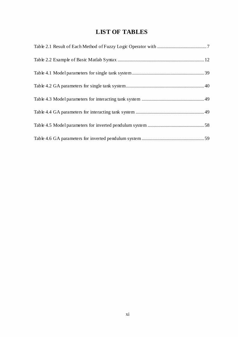
LIST OF TABLES
Table 2.1 Result of Each Method of Fuzzy Logic Operator with ......................................... 7
Table 2.2 Example of Basic Matlab Syntax ........................................................................ 12
Table 4.1 Model parameters for single tank system ............................................................ 39
Table 4.2 GA parameters for single tank system................................................................. 40
Table 4.3 Model parameters for interacting tank system .................................................... 49
Table 4.4 GA parameters for interacting tank system ......................................................... 49
Table 4.5 Model parameters for inverted pendulum system ............................................... 58
Table 4.6 GA parameters for inverted pendulum system .................................................... 59

xii
LIST OF ABBREVIATIONS
DB : Data Base
FLC : Fuzzy Logic Controller
GA : Genetic Algorithm
KB : Knowledge Base
RB : Rule Base
President University 1
CHAPTER 1
INTRODUCTION
1.1. Background of the Final Project
Fuzzy Logic Controller (FLC) has proven its achievement in many real-world control
areas. The Knowledge Base (KB) of these controllers make use of the trade off between
the Data Base (DB) which consists of the scaling factors and the membership function of
the fuzzy sets specifying the meaning of the linguistic terms and the Rule Base (RB)
constituted by the collection of fuzzy rules which defines the relation between input and
output [1]. The drawback of these controllers is the dependency to the experts knowledge
to construct DB and RB which could be a problem when a controller needs to be designed
where the experts knowledge is minimum.
1.2. Problem Statement
Aside from their robustness and their capability in handling the imprecision, FLCs
when conventionally designed, have a high dependency to the presence of experts
knowledge. This drawback is a problem when there is no adequate experts knowledge to
construct the controller, such as in remote area. Therefore, there is a need to provide a
method in which an FLC can be constructed with the minimum involvement of experts.
1.3. Final Project Objective
The Objective of this project is to provide a method to construct FLCs by using the
expert knowledge as minimum as possible while still maintaining the ability to fulfill the
specified task. Genetic Algorithm (GA) is integrated into the design process to achieve this
objective.

President University 2
1.4. Final Project Scope and Limitations
This final project presents a new approach in integrating GA into the design of FLC.
Some ideas from several existing researches will be combined with some original ideas
from the author. This final project itself will focus on the generality of the presented
method. Therefore, three different plants will be used to test the method. The Approximate
Knowledge Base with isosceles triangle shaped membership functions is used in all
designs. All coding is done in MATLAB 7.0.
In the development of this project, there are some limitations:
1) The design process will not be entirely independent on human expert. Expert
knowledge is still used in determining the parameters below:
a. General information of the plant. It consists of inputs, outputs, plant design, plant
constraints, and plant objective.
b. Range of the membership function to be designed (scaling factors).
c. Number of maximum rules per system to be evolved.
d. The Genetic Algorithms parameters such as number of populations, population
boundary, crossover and mutation rate, selection criteria, termination criteria,
crossover, mutation, selection function, etc.
2) Due to the time constraints, this final project will only present the result of each
plant’s test with a certain combinations of the above mentioned parameters. Furthe r
research can be developed to investigate the effect in varying those parameters.
1.5. Final Project Outline
The outline of this final project is as follows:
CHAPTER 1 INTRODUCTION
This chapter consists of the background of the final project, problem statement, final
project objective, final project scope and limitation, and the final project outline
President University 3
CHAPTER 2 LITERATURE STUDY
This chapter presents the explanation on the fuzzy logic system, MATLAB 7.0 as
the programming language, and Genetic Algorithm which will be used to generate fuzzy
controller.
CHAPTER 3 FINAL PROJECT DEVELOPMENT
This chapter presents the design process of the method to generate fuzzy logic
controller automatically by using genetic algorithm.
CHAPTER 4 RESULTS AND DISCUSSION
This chapter shows the result of the proposed method. It is tested in the three plants.
CHAPTER 5 CONCLUSION AND FUTURE WORKS
This is the last chapter of the final project which will conclude the results o f the final
project and potential improvement for future works.
President University 4
CHAPTER 2
LITERATURE STUDY
2.1. Preliminary Remarks
This chapter describes the theories, tools, or methods that are used to support the
project. There are three main components presented in this chapter:
1) Fuzzy Logic System
2) MATLAB 7.0
3) Genetic Algorithm
2.2. Fuzzy Logic System
In short, Fuzzy Logic is a type of logic which incorporates the ability to deal with the
uncertainty/imprecision [7]. The explanation in this section will cover fuzzy set,
membership function, fuzzy logic operator, Fuzzy Inference System (FIS), and Fuzzy
Inference Process.
2.2.1. Fuzzy Sets
In the classical set (crisp set) of bivalent logic, the whole universe of discourse is
only partitioned into two values, either zero (0) or one (1) . On the other hand, fuzzy set is
comprised of a certain membership degree between (0) and (1) [7]. Consider the case of
the height of several people. For example, let a height of 176 cm as a borderline between
‘short’ and ‘tall’ classification. In classical set, it means that someone whose height is 172
cm is considered as short. The fuzzy set, on the other hand, sees this person as ‘tall to a
degree of 0.2’. Figure 2.2 shows the visualization of this case.
President University 5
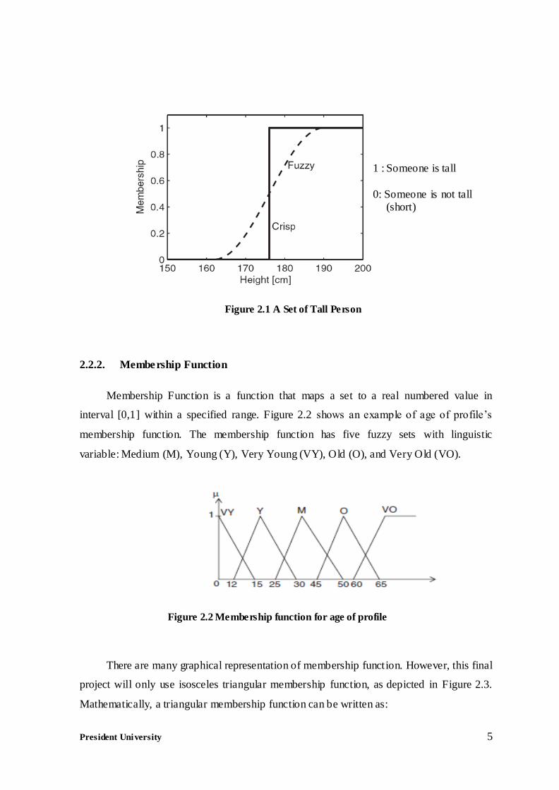
2.2.2. Membership Function
Membership Function is a function that maps a set to a real numbered value in
interval [0,1] within a specified range. Figure 2.2 shows an example of age of profile’s
membership function. The membership function has five fuzzy sets with linguistic
variable: Medium (M), Young (Y), Very Young (VY), Old (O), and Very Old (VO).
Figure 2.2 Membership function for age of profile
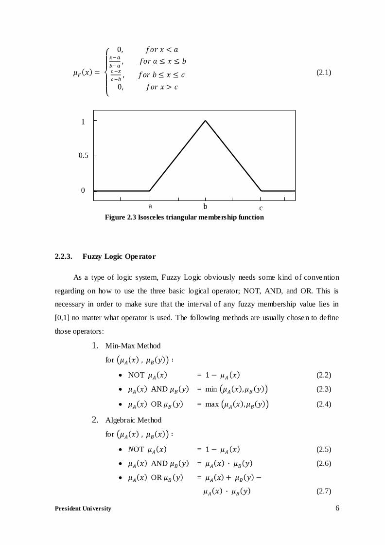
There are many graphical representation of membership function. However, this final
project will only use isosceles triangular membership function, as depicted in Figure 2.3.
Mathematically, a triangular membership function can be written as:
1 : Someone is tall
0: Someone is not tall (short)
Figure 2.1 A Set of Tall Person
President University 6
(2.1)
2.2.3. Fuzzy Logic Operator
As a type of logic system, Fuzzy Logic obviously needs some kind of convention
regarding on how to use the three basic logical operator; NOT, AND, and OR. This is
necessary in order to make sure that the interval of any fuzzy membership value lies in
[0,1] no matter what operator is used. The following methods are usually chose n to define
those operators:
1. Min-Max Method
for
NOT = (2.2)
AND = min (2.3)
OR = max (2.4)
2. Algebraic Method
for
NOT = (2.5)
AND = (2.6)
OR =
(2.7)
c b a
0
1
0.5
Figure 2.3 Isosceles triangular membership function
President University 7
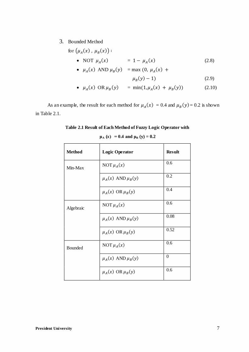
3. Bounded Method
for
NOT = (2.8)
AND =
(2.9)
OR = (2.10)
As an example, the result for each method for = 0.4 and = 0.2 is shown
in Table 2.1.
Table 2.1 Result of Each Method of Fuzzy Logic Operator with
μA (x) = 0.4 and μB (y) = 0.2
Method Logic Operator Result
Min-Max NOT
0.6
AND 0.2
OR 0.4
Algebraic NOT
0.6
AND 0.08
OR 0.52
Bounded NOT
0.6
AND 0
OR 0.6
President University 8
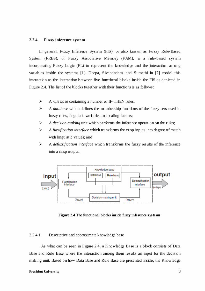
2.2.4. Fuzzy inference system
In general, Fuzzy Inference System (FIS), or also known as Fuzzy Rule-Based
System (FRBS), or Fuzzy Associative Memory (FAM), is a rule-based system
incorporating Fuzzy Logic (FL) to represent the knowledge and the interaction among
variables inside the systems [1]. Deepa, Sivanandam, and Sumathi in [7] model this
interaction as the interaction between five functional blocks inside the FIS as depicted in
Figure 2.4. The list of the blocks together with their functions is as follows:
A rule base containing a number of IF-THEN rules;
A database which defines the membership functions of the fuzzy sets used in
fuzzy rules, linguistic variable, and scaling factors;
A decision-making unit which performs the inference operation on the rules;
A fuzzification interface which transforms the crisp inputs into degree of match
with linguistic values; and
A defuzzification interface which transforms the fuzzy results of the inference
into a crisp output.
Figure 2.4 The functional blocks inside fuzzy inference systems
2.2.4.1. Descriptive and approximate knowledge base
As what can be seen in Figure 2.4, a Knowledge Base is a block consists of Data
Base and Rule Base where the interaction among them results an input for the decision
making unit. Based on how Data Base and Rule Base are presented inside, the Knowledge
President University 9
Base can be categorized into two models [1]. The following subsection briefly explains
them.
1. Descriptive Knowledge Base
A descriptive KB is a KB in which the fuzzy sets giving meaning to the linguistic
labels are uniformly defined for all rules in the RB [1]. In other words, the linguistic
variables take their values as membership function from a global term set defined in
Data Base (DB).
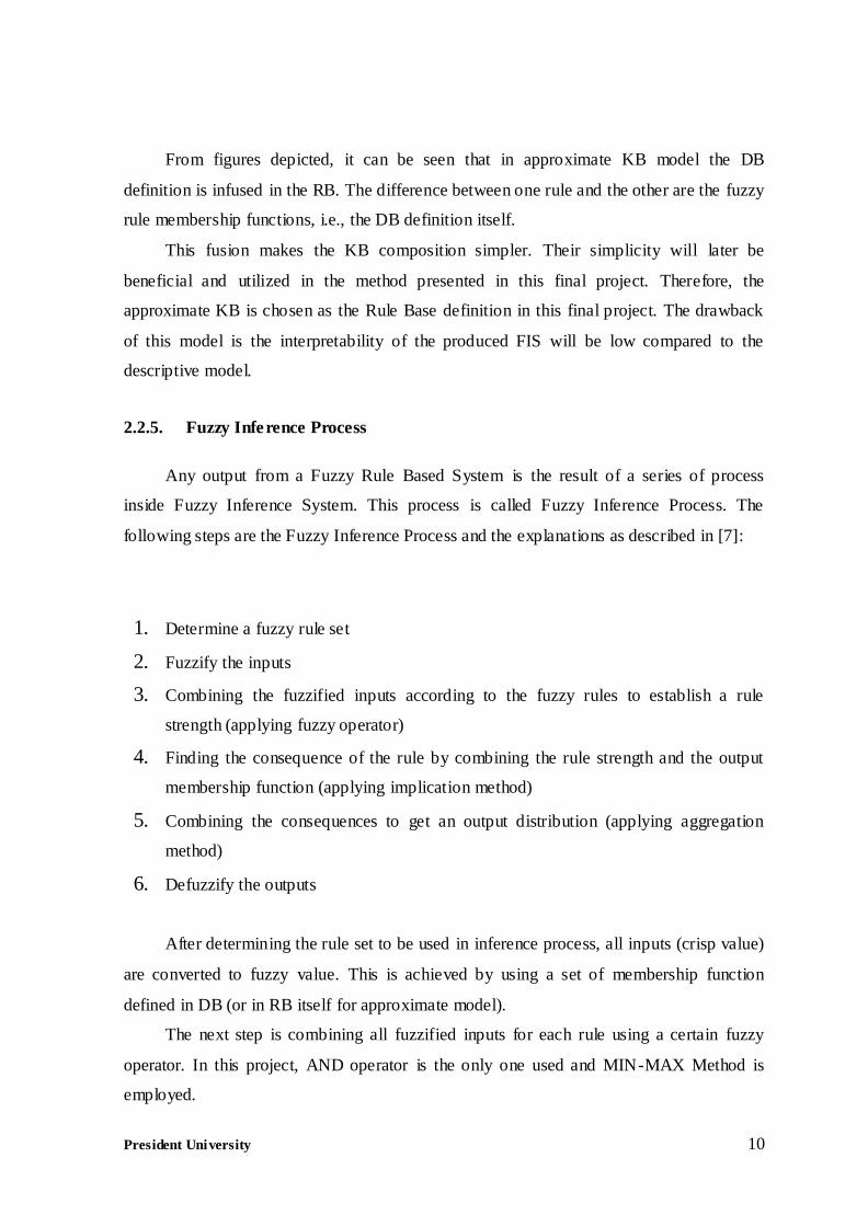
2. Approximate Knowledge Base
In Approximate model, each linguistic variable involved in the rules do not take their
values from a global term set, i.e. each linguistic variable in a fuzzy rule presents its
own meaning.
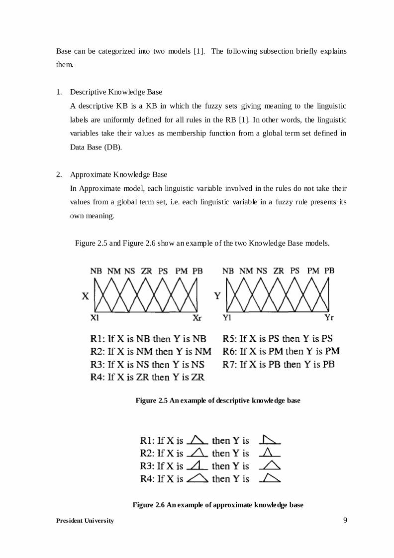
Figure 2.5 and Figure 2.6 show an example of the two Knowledge Base models.
Figure 2.5 An example of descriptive knowledge base
Figure 2.6 An example of approximate knowledge base
President University 10
From figures depicted, it can be seen that in approximate KB model the DB
definition is infused in the RB. The difference between one rule and the other are the fuzzy
rule membership functions, i.e., the DB definition itself.
This fusion makes the KB composition simpler. Their simplicity will later be
beneficial and utilized in the method presented in this final project. Therefore, the
approximate KB is chosen as the Rule Base definition in this final project. The drawback
of this model is the interpretability of the produced FIS will be low compared to the
descriptive model.
2.2.5. Fuzzy Inference Process
Any output from a Fuzzy Rule Based System is the result of a series of process
inside Fuzzy Inference System. This process is called Fuzzy Inference Process. The
following steps are the Fuzzy Inference Process and the explanations as described in [7]:
1. Determine a fuzzy rule set
2. Fuzzify the inputs
3. Combining the fuzzified inputs according to the fuzzy rules to establish a rule
strength (applying fuzzy operator)
4. Finding the consequence of the rule by combining the rule strength and the output
membership function (applying implication method)
5. Combining the consequences to get an output distribution (applying aggregation
method)
6. Defuzzify the outputs
After determining the rule set to be used in inference process, all inputs (crisp value)
are converted to fuzzy value. This is achieved by using a set of membership function
defined in DB (or in RB itself for approximate model).
The next step is combining all fuzzified inputs for each rule using a certain fuzzy
operator. In this project, AND operator is the only one used and MIN-MAX Method is
employed.
President University 11
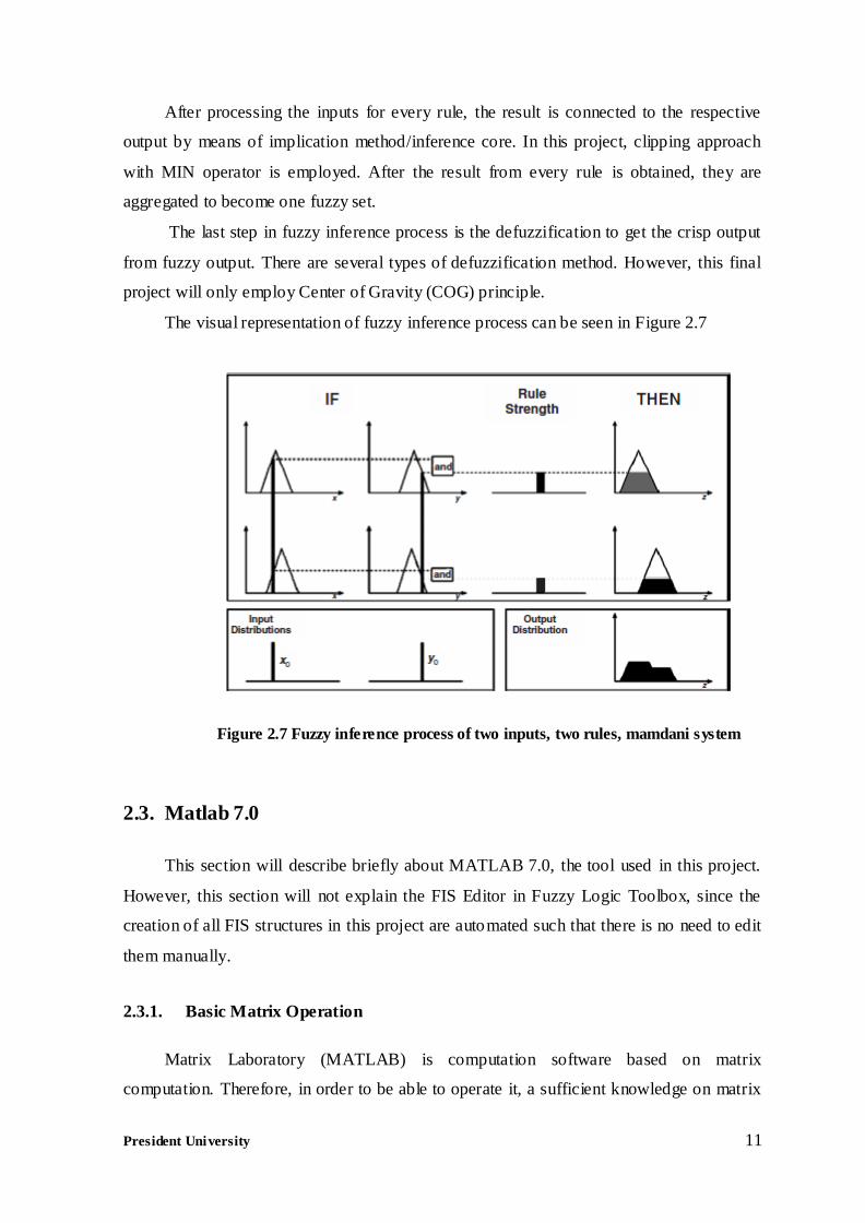
After processing the inputs for every rule, the result is connected to the respective
output by means of implication method/inference core. In this project, clipping approach
with MIN operator is employed. After the result from every rule is obtained, they are
aggregated to become one fuzzy set.
The last step in fuzzy inference process is the defuzzification to get the crisp output
from fuzzy output. There are several types of defuzzification method. However, this final
project will only employ Center of Gravity (COG) principle.
The visual representation of fuzzy inference process can be seen in Figure 2.7
Figure 2.7 Fuzzy inference process of two inputs, two rules, mamdani system
2.3. Matlab 7.0
This section will describe briefly about MATLAB 7.0, the tool used in this project.
However, this section will not explain the FIS Editor in Fuzzy Logic Toolbox, since the
creation of all FIS structures in this project are automated such that there is no need to edit
them manually.
2.3.1. Basic Matrix Operation
Matrix Laboratory (MATLAB) is computation software based on matrix
computation. Therefore, in order to be able to operate it, a sufficient knowledge on matrix
President University 12
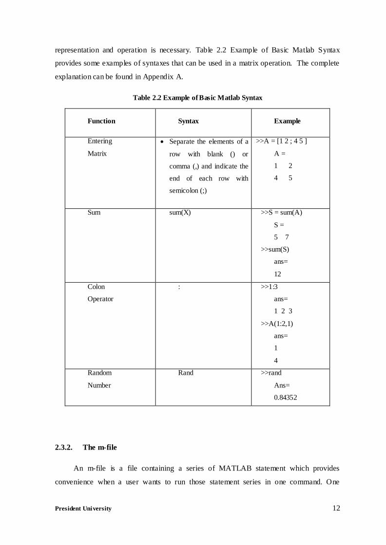
representation and operation is necessary. Table 2.2 Example of Basic Matlab Syntax
provides some examples of syntaxes that can be used in a matrix operation. The complete
explanation can be found in Appendix A.
Table 2.2 Example of Basic Matlab Syntax
Function Syntax Example
Entering
Matrix
Separate the elements of a
row with blank () or
comma (,) and indicate the
end of each row with
semicolon (;)
>>A = [1 2 ; 4 5 ]
A =
1 2
4 5
Sum sum(X) >>S = sum(A)
S =
5 7
>>sum(S)
ans=
12
Colon
Operator
: >>1:3
ans=
1 2 3
>>A(1:2,1)
ans=
1
4
Random
Number
Rand >>rand
Ans=
0.84352
2.3.2. The m-file
An m-file is a file containing a series of MATLAB statement which provides
convenience when a user wants to run those statement series in one command. One
President University 13
obvious characteristic of m-file is the extension (.m). MATLAB m-file can be made by a
text editor.
m-file can be categorized into two types:
1. Scripts, which neither accept input arguments nor return output argument.
2. Functions, which can either accept input argument or return output argument.
Another difference between these two m-file is that a function stores its variables in
workspace that is local to the function [9].
Any variable produced by scripts m- file will be stored in MATLAB’s base
workspace. For example, consider a script m- file named “trialscript.m” which contains
MATLAB statements as follows:
m = n*2
Initialize n in MATLAB command window and then called “trialscript”. The result
will be displayed as:
>> n = [2 3]
n =
2 3
>>trialscript
m=
4 6
On the other hand, functions save their variables in their local workspace, i.e. it
cannot be read directly from MATLAB base workspace. To communicate the variable
from function to MATLAB workspace or other function workspace, certain assignment
syntax is required. The assignment is written according to the following format:
Function [out1, out2, ...] = function_name (inp1, inp2, ...)
President University 14
For example, consider a function m- file named “testfunction.m” contains the
following statements:
function [z] = testfunction (x,y)
z = x+y
When a user call “testfunction.m” with the appropriate inputs, the display in
MATLAB window will be:
>>testfunction(2,7)
z =
9
Ans =
9
>>who
Ans
After the execution of “testfunction.m”, the variable used in the function is stored in
local workspace, not in MATLAB base workspace. Therefore, the variable read in
MATLAB base workspace is only “Ans”.
2.3.3. Simulink
Simulink is a software package for modeling, simulating, and analyzing dynamical
systems [6]. Simulink provides flexibility in designing model with so many model blocks.
The model created in simulink will be saved by MATLAB with the extension ‘.mdl’. This
section will only give a brief explanation on how to start creating a model in simulink.
2.3.3.1. Simulink library browser
In order to open Simulink, a user only needs to type simulink in MATLAB command
window. This will open simulink library browser as in Figure 2.8 from where the user can
get the blocks needed for the model.
President University 15
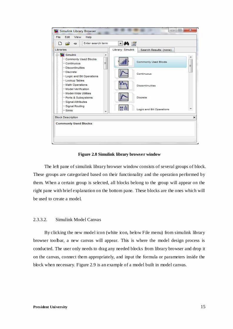
Figure 2.8 Simulink library browser window
The left pane of simulink library browser window consists of several groups of block.
These groups are categorized based on their functionality and the operation performed by
them. When a certain group is selected, all blocks belong to the group will appear on the
right pane with brief explanation on the bottom pane. These blocks are the ones which will
be used to create a model.
2.3.3.2. Simulink Model Canvas
By clicking the new model icon (white icon, below File menu) from simulink library
browser toolbar, a new canvas will appear. This is where the model design process is
conducted. The user only needs to drag any needed blocks from library browser and drop it
on the canvas, connect them appropriately, and input the formula or parameters inside the
block when necessary. Figure 2.9 is an example of a model built in model canvas.
President University 16
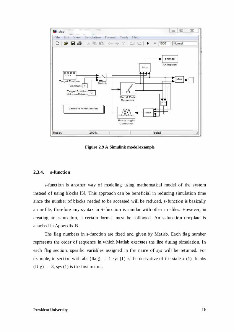
Figure 2.9 A Simulink model example
2.3.4. s-function
s-function is another way of modeling using mathematical model of the system
instead of using blocks [5]. This approach can be beneficial in reducing simulation time
since the number of blocks needed to be accessed will be reduced. s- function is basically
an m-file, therefore any syntax in S-function is similar with other m -files. However, in
creating an s-function, a certain format must be followed. An s- function template is
attached in Appendix B.
The flag numbers in s- function are fixed and given by Matlab. Each flag number
represents the order of sequence in which Matlab executes the line during simulation. In
each flag section, spesific variables assigned in the name of sys will be returned. For
example, in section with abs (flag) == 1 sys (1) is the derivative of the state x (1). In abs
(flag) == 3, sys (1) is the first output.
President University 17
2.4. Genetic Algorithm
Genetic Algorithm is an optimization algorithm which mimics the biological nature
involving reproduction, natural selection, mutation, etc. Genetic Algorithm (GA), through
its development as an optimization algorithm reaches success due to its ability to find
solution to a problem even from random initial guess in a large search space [8].
The basic idea of GA is the ‘survival of the fittest,’ or ‘nature selection’. It means
that only a certain individual (solution candidate) who is fit enough (translated as it can
give result close to the objective function) can survive to the next generation. It is
understandable that a fit individual is highly possible to have good traits. Therefore, by
allowing this individual to produce the next generation, it is possible that the next
generation will also have comparably good fitness. In other words, theore tically, the
collection of solution candidate’s quality will improve from generation to generation.
2.4.1. Genetic Algorithm Terminologies
As an algorithm which was inspired by nature, Genetic Algorithm incorporates some
terminology from biology for its process and for the operators involved in the process. In
order to understand more of its nature, this section explains briefly some of those
terminologies.
1. Individual.
A candidate of solution of the problem, usually represented by a Chromosome.
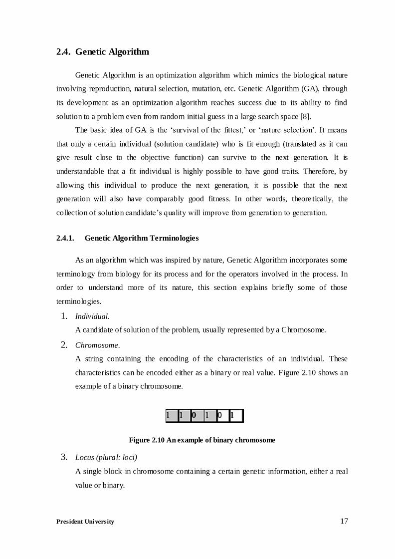
2. Chromosome.
A string containing the encoding of the characteristics of an individual. These
characteristics can be encoded either as a binary or real value. Figure 2.10 shows an
example of a binary chromosome.
Figure 2.10 An example of binary chromosome
3. Locus (plural: loci)
A single block in chromosome containing a certain genetic information, either a real
value or binary.
President University 18
4. Gene
A genetic information in locus. It can be represented by either bit of binary or real
value.
5. Genotype
A raw string encoded in chromosome. The content of genotype is just a string of
code, without any meaning before being translated by a certain function. Genotype
still cannot be evaluated yet in evaluator, except the genotype is already the
phenotype itself, as in some cases of real-valued GA.
6. Phenotype
The translated version of the genotype. For example, chromosome in
Figure 2.10 has genotype 110101, therefore the phenotype is 53 if the translator is
binary to real number function. The one passed to the evaluator is usually Phenotype.
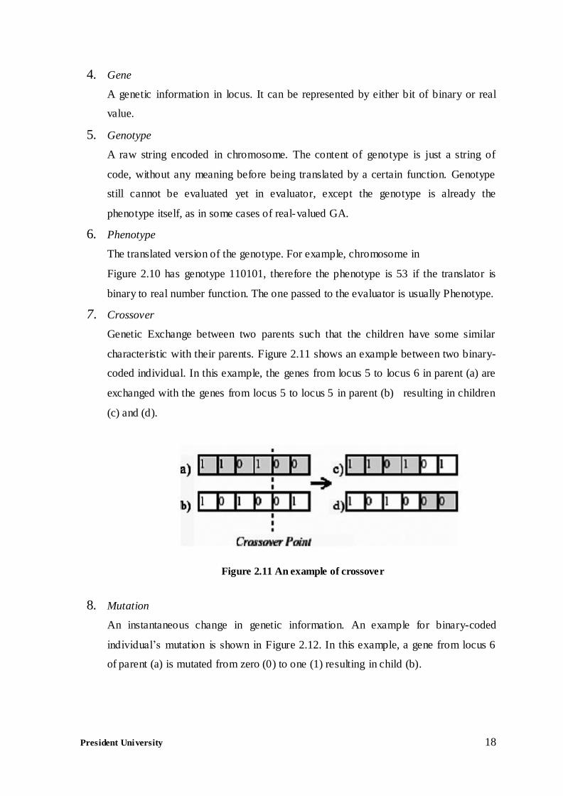
7. Crossover
Genetic Exchange between two parents such that the children have some similar
characteristic with their parents. Figure 2.11 shows an example between two binary-
coded individual. In this example, the genes from locus 5 to locus 6 in parent (a) are
exchanged with the genes from locus 5 to locus 5 in parent (b) resulting in children
(c) and (d).
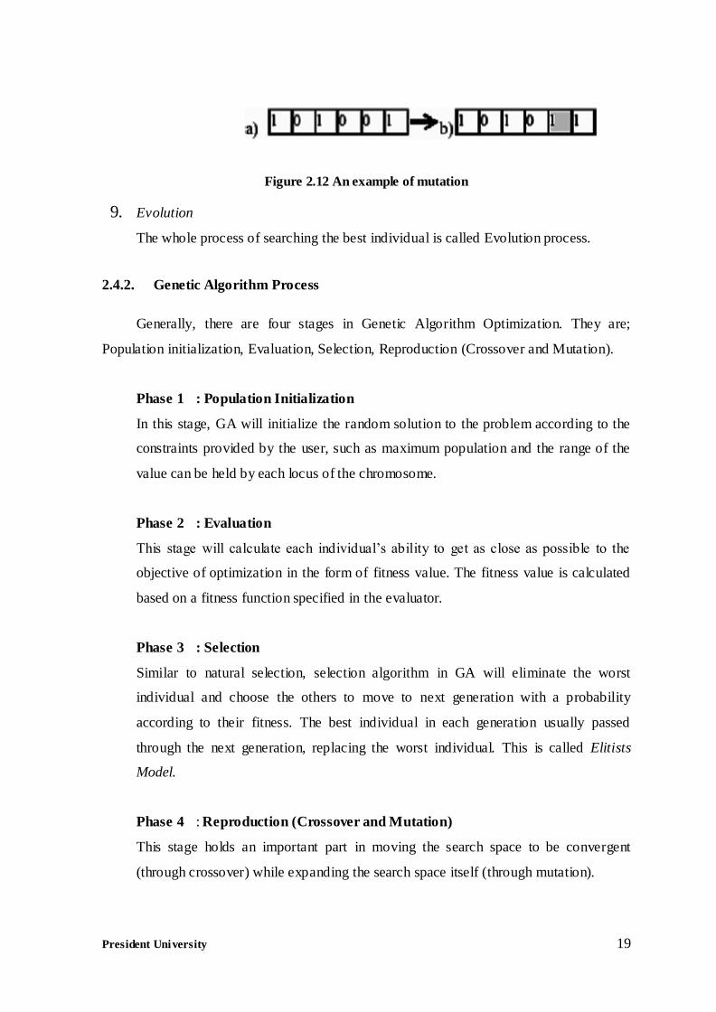
8. Mutation
An instantaneous change in genetic information. An example for binary-coded
individual’s mutation is shown in Figure 2.12. In this example, a gene from locus 6
of parent (a) is mutated from zero (0) to one (1) resulting in child (b).
Figure 2.11 An example of crossover
President University 19
Figure 2.12 An example of mutation
9. Evolution
The whole process of searching the best individual is called Evolution process.
2.4.2. Genetic Algorithm Process
Generally, there are four stages in Genetic Algorithm Optimization. They are;
Population initialization, Evaluation, Selection, Reproduction (Crossover and Mutation).
Phase 1 : Population Initialization
In this stage, GA will initialize the random solution to the problem according to the
constraints provided by the user, such as maximum population and the range of the
value can be held by each locus of the chromosome.
Phase 2 : Evaluation
This stage will calculate each individual’s ability to get as close as possible to the
objective of optimization in the form of fitness value. The fitness value is calculated
based on a fitness function specified in the evaluator.
Phase 3 : Selection
Similar to natural selection, selection algorithm in GA will eliminate the worst
individual and choose the others to move to next generation with a probability
according to their fitness. The best individual in each generation usually passed
through the next generation, replacing the worst individual. This is called Elitists
Model.
Phase 4 : Reproduction (Crossover and Mutation)
This stage holds an important part in moving the search space to be convergent
(through crossover) while expanding the search space itself (through mutation).
President University 20
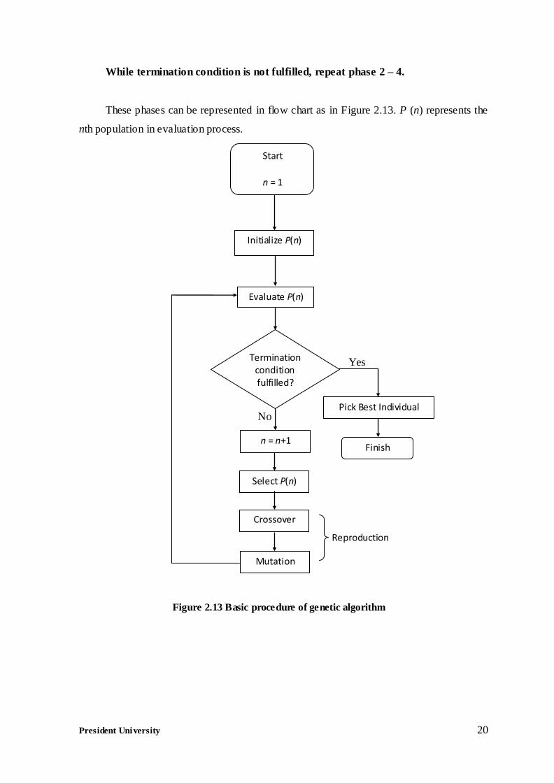
While termination condition is not fulfilled, repeat phase 2 – 4.
These phases can be represented in flow chart as in Figure 2.13. P (n) represents the
nth population in evaluation process.
Mutation
Reproduction
No
n = n+1
Yes Termination condition fulfilled?
Evaluate P(n)
Initialize P(n)
Start
n = 1
Pick Best Individual
Select P(n)
Crossover
Finish
Figure 2.13 Basic procedure of genetic algorithm
President University 21
CHAPTER 3
FINAL PROJECT DEVELOPMENT
3.1. Preliminary Remarks
This chapter will describe the development of the final project. This final project
integrates several ideas into the basic genetic algorithm which is already explained in
chapter 2. Therefore, this chapter will focus on the development of the ideas and the
construction of the m-files to realize those ideas.
3.2. Concept Development
This section will describe in details the population encoding method, the process
flow the modified genetic algorithm followed by its explanations, and the explanations on
GA parameters.
3.2.1. Population Encoding
Population encoding is one of the important aspect in genetic algorithm. The
encoding must be compact while still represents the behavior of the individual [3]. Every
encoding in this project uses real-valued encoding instead of binary encoding. The reasons
behind this decision are:
1. To keep the length of the chromosome as small as possible. Consider the encoding of
integer ‘5’. In real valued encoding this one value will take only one locus, while in
binary it is translated as ‘101’ and thus used three loci.
2. To make the interpretability of the chromosome higher and the coding process easier.
3. To avoid unnecessary chromosome. Consider a set of population consists of 25
individuals. The length of binary string needed to encode this is 5 bits. However,
since 25 = 32, there will be 7 unnecessary chromosomes. In order to handle these
chromosomes, usually there are two approaches that can be applied. The first,
interpret these chromosomes as invalid values. However, this approach will show
President University 22
how inefficient the coding is. The second approach uses these chromosomes to
represent the existing phenotypes (number 1 to 25). Therefore, some of the
phenotypes might have more than one representation. This is unfair since those
phenotypes will have higher chance to appear in any generation because of multiple
representations.
In order to make the failure tracking in coding easier, this final project uses three
stages of encoding as follows:
A. Preliminary Encoding
This encoding is used in the earliest phase of GA process. The idea is taken from [3].
Each chromosome in this stage represents exactly one rule. This encoding comprises
two parts, the center point and the half-base width (the length from center to either
base point) of the input and output membership functions. Thus, each chromosome
is 2*(input+out) in length. Figure 3.1 visualize this representation.
Cooper and Vidal in [3] limits the half-base width in the range of [15%, 85%] of the
membership function’s universe of discourse. This is to avoid the occurrence of
unimportant variables and over-dominant variables. This final project applies the
range of [15%, 80%].
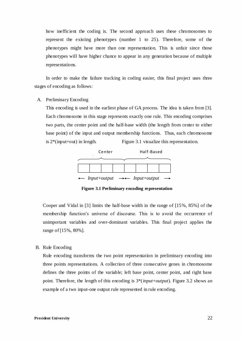
B. Rule Encoding
Rule encoding transforms the two point representation in preliminary encoding into
three points representations. A collection of three consecutive genes in chromosome
defines the three points of the variable; left base point, center point, and right base
point. Therefore, the length of this encoding is 3*( input+output). Figure 3.2 shows an
example of a two input-one output rule represented in rule encoding.
Center points
Hal f -Based Width
Input+output Input+output
Figure 3.1 Preliminary encoding representation
President University 23
It should be noted that rule encoding is the one used in gene pool, the database of all
genetic material used throughout GA process.
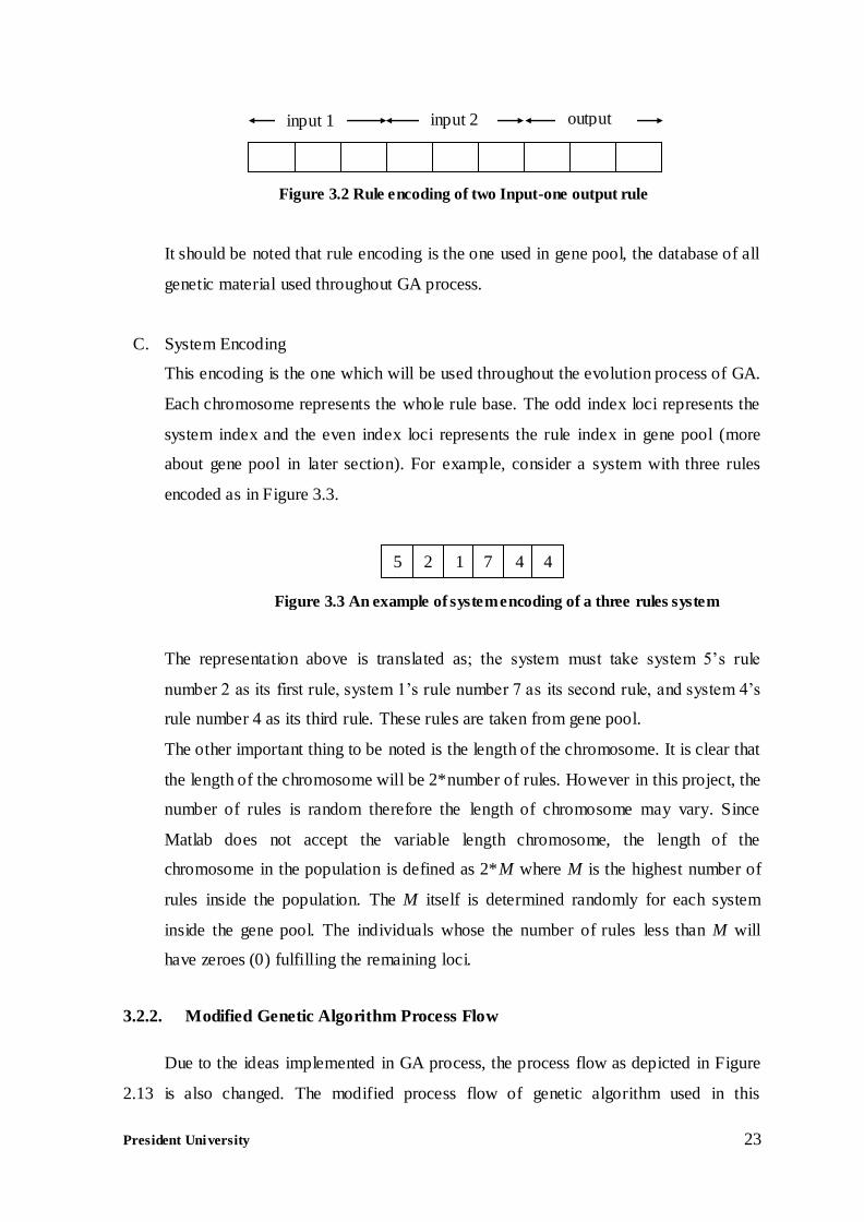
C. System Encoding
This encoding is the one which will be used throughout the evolution process of GA.
Each chromosome represents the whole rule base. The odd index loci represents the
system index and the even index loci represents the rule index in gene pool (more
about gene pool in later section). For example, consider a system with three rules
encoded as in Figure 3.3.
The representation above is translated as; the system must take system 5’s rule
number 2 as its first rule, system 1’s rule number 7 as its second rule, and system 4’s
rule number 4 as its third rule. These rules are taken from gene pool.
The other important thing to be noted is the length of the chromosome. It is clear that
the length of the chromosome will be 2*number of rules. However in this project, the
number of rules is random therefore the length of chromosome may vary. Since
Matlab does not accept the variable length chromosome, the length of the
chromosome in the population is defined as 2*M where M is the highest number of
rules inside the population. The M itself is determined randomly for each system
inside the gene pool. The individuals whose the number of rules less than M will
have zeroes (0) fulfilling the remaining loci.
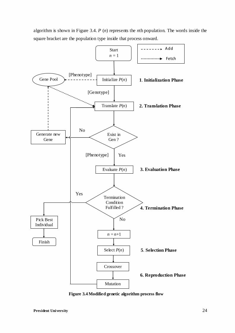
3.2.2. Modified Genetic Algorithm Process Flow
Due to the ideas implemented in GA process, the process flow as depicted in Figure
2.13 is also changed. The modified process flow of genetic algorithm used in this
input 1 input 2 output
5 2 1 7 4 4
Figure 3.2 Rule encoding of two Input-one output rule
Figure 3.3 An example of system encoding of a three rules system
President University 24
algorithm is shown in Figure 3.4. P (n) represents the nth population. The words inside the
square bracket are the population type inside that process onward.
Figure 3.4 Modified genetic algorithm process flow
Add
Fetch
Yes
No
No
4. Termination Phase
3. Evaluation Phase
6. Reproduction Phase
5. Selection Phase
Finish
Pick Best Individual
Termination Condition Fulfilled ?
Evaluate P(n)
Mutation
Crossover
Select P(n)
n = n+1
[Phenotype] Yes
Generate new
Gene Exist in Gen ?
Pool?
2. Translation Phase Translate P(n)
[Genotype]
Gene Pool [Phenotype]
Start
n = 1
Initialize P(n) 1. Initialization Phase
President University 25
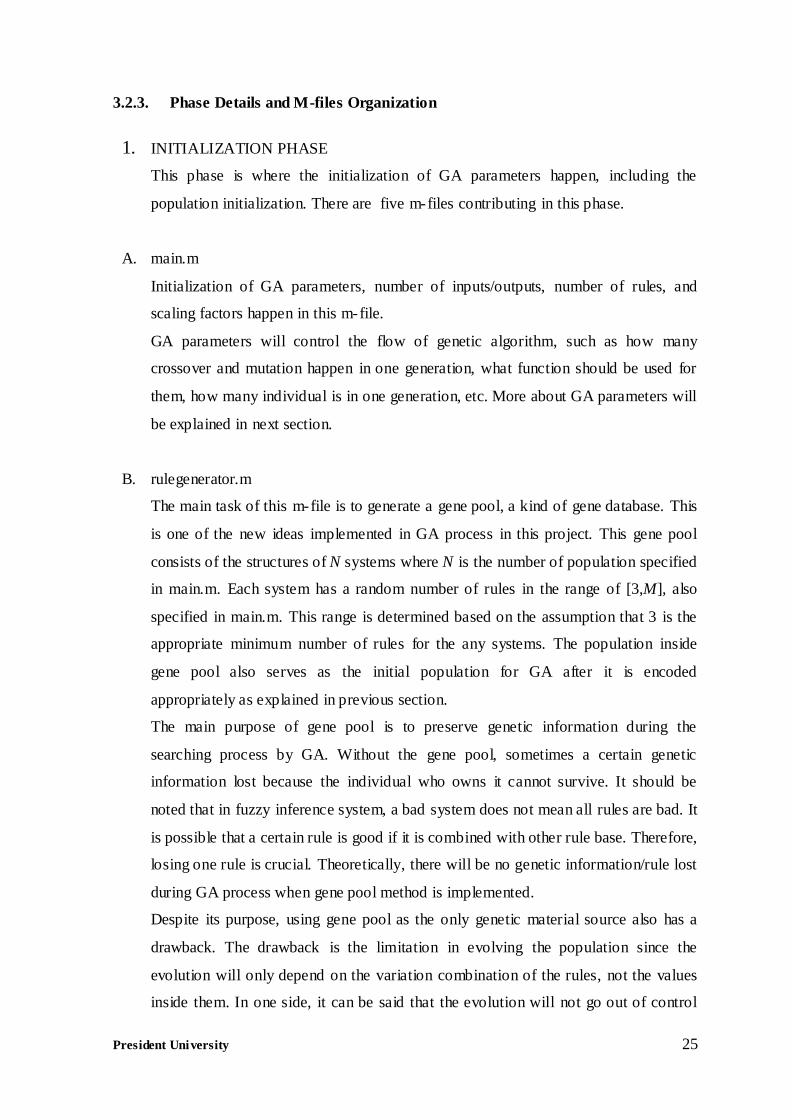
3.2.3. Phase Details and M-files Organization
1. INITIALIZATION PHASE
This phase is where the initialization of GA parameters happen, including the
population initialization. There are five m-files contributing in this phase.
A. main.m
Initialization of GA parameters, number of inputs/outputs, number of rules, and
scaling factors happen in this m-file.
GA parameters will control the flow of genetic algorithm, such as how many
crossover and mutation happen in one generation, what function should be used for
them, how many individual is in one generation, etc. More about GA parameters will
be explained in next section.
B. rulegenerator.m
The main task of this m-file is to generate a gene pool, a kind of gene database. This
is one of the new ideas implemented in GA process in this project. This gene pool
consists of the structures of N systems where N is the number of population specified
in main.m. Each system has a random number of rules in the range of [3,M], also
specified in main.m. This range is determined based on the assumption that 3 is the
appropriate minimum number of rules for the any systems. The population inside
gene pool also serves as the initial population for GA after it is encoded
appropriately as explained in previous section.
The main purpose of gene pool is to preserve genetic information during the
searching process by GA. Without the gene pool, sometimes a certain genetic
information lost because the individual who owns it cannot survive. It should be
noted that in fuzzy inference system, a bad system does not mean all rules are bad. It
is possible that a certain rule is good if it is combined with other rule base. Therefore,
losing one rule is crucial. Theoretically, there will be no genetic information/rule lost
during GA process when gene pool method is implemented.
Despite its purpose, using gene pool as the only genetic material source also has a
drawback. The drawback is the limitation in evolving the population since the
evolution will only depend on the variation combination of the rules, not the values
inside them. In one side, it can be said that the evolution will not go out of control

President University 26
because of this limitation, but on the other hand it cannot be avoided that the
evolution can be slow, especially when using small population and small number of
rules. However, this drawback can be reduced by the mutation function developed
for this final project, which will be explained later.
C. rulecomposer.m
The task of rule composer is to encode each rule generated by rulegenerator into
three point representation for each variable. The three points represents the left base
point, center point, and right base point of the isosceles triangular membership
function.
D. rulefilter.m
rulefilter holds the responsibility in making the rule base as efficient as possible.
Since this m-file mostly works in translation phase, the complete explanation on how
rulefilter can fulfill its responsibility will be delivered in the said phase later.
E. initga.m
initga will process the system-encoded initial population from rulegenerator by
attaching initial fitness value (usually zero) at the end of each chromosome.
2. TRANSLATION PHASE
The task of this phase is the translation from system-encoded chromosome into the
rule-encoded chromosome to be used in evaluator. This is done by fetching the
genetic materials (rules) from gene pool as the one implied in system-encoded
chromosome. There are two m-files in this phase.
A. translator.m
The main part of translation phase. It translates the incoming chromosome (system-
encoded) and returns the rule base in form of rule-encoded chromosomes.
B. rulefilter.m
This m-file is another idea implemented in the project. It holds an important duty in
processing the incoming rule base to be as compact as possible.
The process inside rulefilter can be categorized in three stages.
President University 27
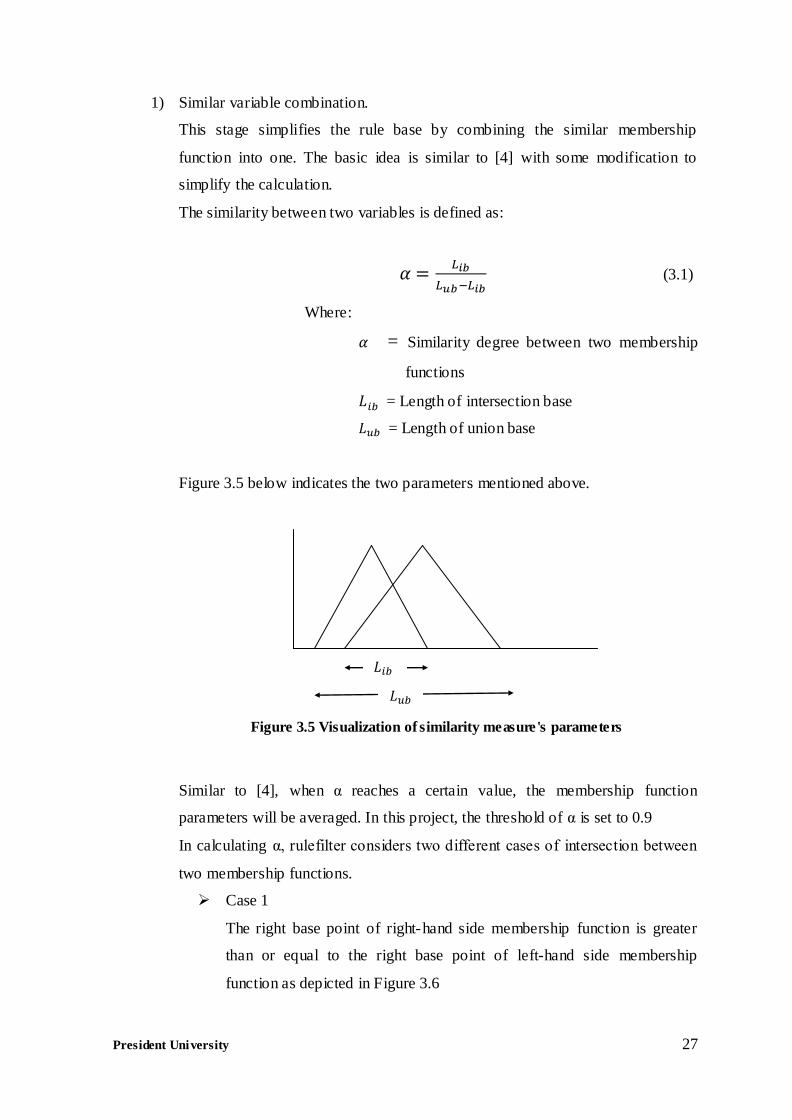
1) Similar variable combination.
This stage simplifies the rule base by combining the similar membership
function into one. The basic idea is similar to [4] with some modification to
simplify the calculation.
The similarity between two variables is defined as:
(3.1)
Where:
= Similarity degree between two membership
functions
= Length of intersection base
= Length of union base
Figure 3.5 below indicates the two parameters mentioned above.
Similar to [4], when α reaches a certain value, the membership function
parameters will be averaged. In this project, the threshold of α is set to 0.9
In calculating α, rulefilter considers two different cases of intersection between
two membership functions.
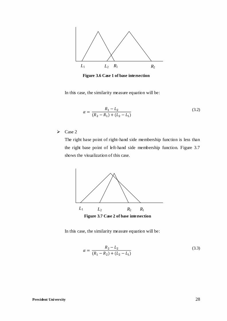
Case 1
The right base point of right-hand side membership function is greater
than or equal to the right base point of left-hand side membership
function as depicted in Figure 3.6
Figure 3.5 Visualization of similarity measure's parameters
President University 28
In this case, the similarity measure equation will be:
(3.2)
Case 2
The right base point of right-hand side membership function is less than
the right base point of left-hand side membership function. Figure 3.7
shows the visualization of this case.
In this case, the similarity measure equation will be:
(3.3)
R1 L2 L1 R2
L1 L2 R2 R1
Figure 3.7 Case 2 of base intersection
Figure 3.6 Case 1 of base intersection
President University 29
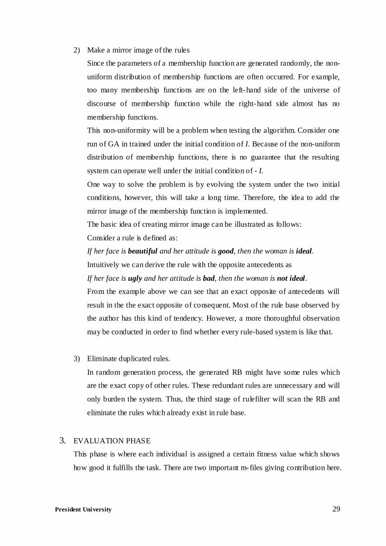
2) Make a mirror image of the rules
Since the parameters of a membership function are generated randomly, the non-
uniform distribution of membership functions are often occurred. For example,
too many membership functions are on the left-hand side of the universe of
discourse of membership function while the right-hand side almost has no
membership functions.
This non-uniformity will be a problem when testing the algorithm. Consider one
run of GA in trained under the initial condition of I. Because of the non-uniform
distribution of membership functions, there is no guarantee that the resulting
system can operate well under the initial condition of - I.
One way to solve the problem is by evolving the system under the two initial
conditions, however, this will take a long time. Therefore, the idea to add the
mirror image of the membership function is implemented.
The basic idea of creating mirror image can be illustrated as follows:
Consider a rule is defined as:
If her face is beautiful and her attitude is good, then the woman is ideal.
Intuitively we can derive the rule with the opposite antecedents as
If her face is ugly and her attitude is bad, then the woman is not ideal.
From the example above we can see that an exact opposite of antecedents will
result in the the exact opposite of consequent. Most of the rule base observed by
the author has this kind of tendency. However, a more thoroughful observation
may be conducted in order to find whether every rule-based system is like that.
3) Eliminate duplicated rules.
In random generation process, the generated RB might have some rules which
are the exact copy of other rules. These redundant rules are unnecessary and will
only burden the system. Thus, the third stage of rulefilter will scan the RB and
eliminate the rules which already exist in rule base.
3. EVALUATION PHASE
This phase is where each individual is assigned a certain fitness value which shows
how good it fulfills the task. There are two important m-files giving contribution here.
President University 30
A. fiscreator.m
This m-file will create the fuzzy inference system based on the incoming rule base
which will be tested on the models. Since this final project uses approximate model
of KB, the number of rules will be the same as the number of membership function
for each variable. Other parameters of the fuzzy inference system are set to default
(Mamdani type, Min-Max method, Min implication method, and COG
defuzzification method).
B. evaluator.m
The fitness value of each individual is assigned here. Firstly, this m-file will extract
the the incoming chromosome and translate it rule base by using translator. It then
create a fis file using fiscreator and then simulate the test models with the generated
fis file attached to fuzzy controller block. The performance for each individual is
calculated by a certain cost function, usually incorporating the errors obtained during
simulation. The number of rules can also be added into the fitness function. It should
be noted that the fitness value is proportional to the performance of the individual.
Thus, the cost function is inverted. The basic form of fitness function used in this
project is therefore:
(3.4)
Where = The fitness value
= The cost function
= Weighting factor
4. TERMINATION PHASE
This phase will check whether the termination condition is met. The termination
condition for every simulation in this final project is when the population reaches the
maximum value. maxGenTerm is used to achieve the purpose. For the sake of
flexibility, another modification is made here. Every time the simulation reaches K
consecutive populations without any improvement of the best individual, the user
may decide to either continue the simulation or terminate it. The maximum
population value in this final project is also not absolute. It means the user can
President University 31
continue the simulation even after reaching the maximum number of population if
the user is still unsatisfied with the result.
5. SELECTION PHASE
The selection of the individual happens here. The selection is conducted by means of
a certain selection algorithm. This final project uses roulette wheel algorithm, thus
the m-file contributing here is roulette.m. More about this selection algorithm
/selection function will be explained thoroughly in later section.
6. REPRODUCTION PHASE
This phase mimics the reproduction of genes in nature. Similar with nature, the
reproduction is carried out by means of crossover and mutation algorithm. This
project uses original crossover and mutation algorithm in form of custxover.m and
custmut.m. In later section these two algorithms will be explained further.
There is one more m-file not yet explained which is run_ga.m. It is not included in
the previous explanation because this m-file works on every phase from phase 2 to
phase 5. It controls the flow of GA, calling appropriate m-file when needed, and
record the progress.
Examples of the series of m-files used in the project are attached in Appendix C. The
complete m-files for each system test, however, will be in the disk attached to this
final project.
3.3. Genetic Algorithm Parameters
In order to fulfill the task at hand, several parameters or algorithms are needed during
GA process. The explanation in this section consists of; Initialization parameters, Selection
function1, Elitist Model, Crossover function, Mutation function, and Termination function.
1 Eventhough it is called ‘function’, this is not a mathematical function by any means. This is just a
common name used to define the algorithms used in GA process (Selection function, Crosso ver function,
Mutation function, etc.).
President University 32
3.3.1. Initialization Parameters
1. Population size
This parameter defines the number of individuals in each generation. Larger
population will make the possibilities to find the best individual in any generation
higher, however the searching process will be slower.
2. Number of inputs and outputs
These parameters are important in deciding the length of each chromosome (see
section 3.2.1). They also holds important factor in determining how fuzzy inference
system will be constructed.
3. Scaling factors
Scaling factors will determine the range of membership function of inputs and
outputs variables. Small scaling factor means the variable will be more sensitive to
changes, but in cost of coverage area. High scaling factor means wider coverage area
but low sensitivity.
4. Number of rules
It will decide the range of the number of rules allowed in each system in gene pool.
This also needs to be considered appropriately since high number of rules will
burden the system while increasing the choices of genetic materials to be taken from
gene pool during evolution.
5. Number of generation
It indicates how long the GA progress will run. The population in the whole process
before selection phase in Figure 3.4 is counted as one generation. The complex
problem usually needs higher value of this parameter.
6. Population boundary
This parameter will limit the value allowed in every locus. In this project, the
boundary for even- indexed locus is [1, population size] while the boundary for odd-
indexed locus is [1, max number of rules].
President University 33
7. Crossover rate
It determines how many crossovers takes place in each generation. Higher rate might
increase the possibility to find the best individual while making the searching process
slower.
8. Mutation rate
Similar to crossover rate, mutation rate determines how many mutations occur in
each generation. Usually it is kept at low value, since high number of mutation will
make GA progress to be just a random search [2].
3.3.2. Selection Function
There are several selection algorithm choices exist, however this section will only
explain the earliest algorithm, roulette wheel selection, since this algorithm is the one used
in this project.
Roulette Wheel Selection.
The basic concept of this algorithm is as follows:
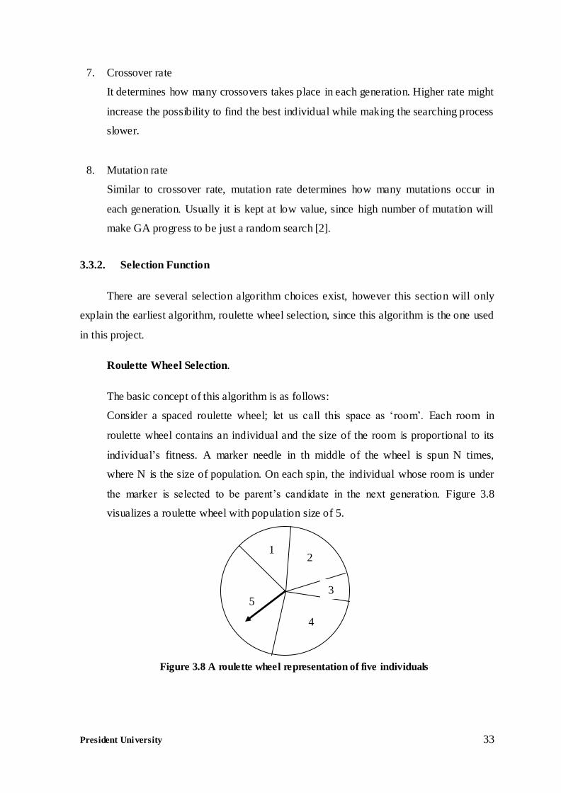
Consider a spaced roulette wheel; let us call this space as ‘room’. Each room in
roulette wheel contains an individual and the size of the room is proportional to its
individual’s fitness. A marker needle in th middle of the wheel is spun N times,
where N is the size of population. On each spin, the individual whose room is under
the marker is selected to be parent’s candidate in the next generation. Figure 3.8
visualizes a roulette wheel with population size of 5.
4
3
2 1
5
Figure 3.8 A roulette wheel representation of five individuals

President University 34
Linkens and Chen in [4] explain the steps taken to realize roulette wheel as
follows:
1) Calculate the expected value of each individual, which is the fitness
of the individual divided by population fitness (total fitness in
population).
2) Sum the total expected value of the individuals in population, let it
be T.
3) Repeat N (the population size) times:
i. Choose a random integer r in [0, T].
ii. Loop through the individuals in population, summing the
expected values, until the sum is greater than or equal to r.
The individual whose expected value puts the sum over this
limit is the one selected. The copy of this individual is taken
to be parent’s candidate.
Roulette wheel selection is the traditional selection algorithm; therefore there are
some flaws inside it. One of the flaw is there is high possibility that the fitter individuals
will dominate the population since the probability that it will be selected is the same in
each spin. However, for a beginner practitioner this algorithm is ideal since it is easy to
understand.
3.3.3. Elitist Model
With selection probability as mentioned before, the best individual in one generation
is not guaranteed to survive. It has high probability to be chosen but it will not be 100%.
The other problem is that in genetic algorithm, every child will replace its parents in next
generation. Therefore, when the best individual is chosen to be a parent, that individual
will not be chosen to proceed to the next generation.
One common method to solve this problem is by using elitist model. In this model,
every time an evaluation phase is finished, the copy of the best individual is preserved.
This copy will later be inserted directly into the next generation directly. The worst
individual is usually sacrificed to provide a place for the best individual.
President University 35
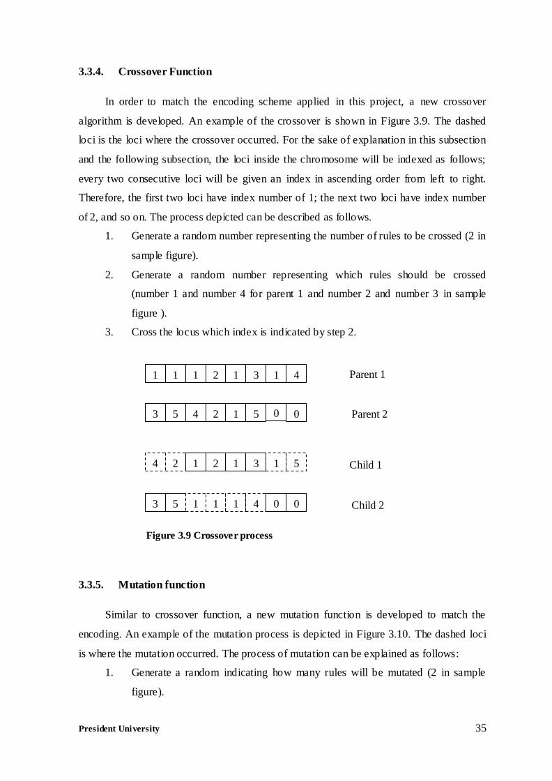
3.3.4. Crossover Function
In order to match the encoding scheme applied in this project, a new crossover
algorithm is developed. An example of the crossover is shown in Figure 3.9. The dashed
loci is the loci where the crossover occurred. For the sake of explanation in this subsection
and the following subsection, the loci inside the chromosome will be indexed as follows;
every two consecutive loci will be given an index in ascending order from left to right.
Therefore, the first two loci have index number of 1; the next two loci have index number
of 2, and so on. The process depicted can be described as follows.
1. Generate a random number representing the number of rules to be crossed (2 in
sample figure).
2. Generate a random number representing which rules should be crossed
(number 1 and number 4 for parent 1 and number 2 and number 3 in sample
figure ).
3. Cross the locus which index is indicated by step 2.
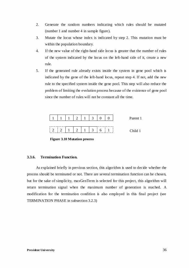
3.3.5. Mutation function
Similar to crossover function, a new mutation function is developed to match the
encoding. An example of the mutation process is depicted in Figure 3.10. The dashed loci
is where the mutation occurred. The process of mutation can be explained as follows:
1. Generate a random indicating how many rules will be mutated (2 in sample
figure).
1 1 1 2 1 3 1 4 Parent 1
3 5 4 2 1 5 Parent 2 0 0
4 2 1 2 1 3 1 5 Child 1
3 5 1 1 1 4 Child 2 0 0
Figure 3.9 Crossover process
President University 36
2. Generate the random numbers indicating which rules should be mutated
(number 1 and number 4 in sample figure).
3. Mutate the locus whose index is indicated by step 2. This mutation must be
within the population boundary.
4. If the new value of the right-hand side locus is greater that the number of rules
of the system indicated by the locus on the left-hand side of it, create a new
rule.
5. If the generated rule already exists inside the system in gene pool which is
indicated by the gene of the left-hand locus, repeat step 4. If not, add the new
rule to the specified system inside the gene pool. This step will also reduce the
problem of limiting the evolution process because of the existence of gene pool
since the number of rules will not be constant all the time.
3.3.6. Termination Function.
As explained briefly in previous section, this algorithm is used to decide whether the
process should be terminated or not. There are several termination function can be chosen,
but for the sake of simplicity, maxGenTerm is selected for this project, this algorithm will
return termination signal when the maximum number of generation is reached. A
modification for the termination condition is also employed in this final project (see
TERMINATION PHASE in subsection 3.2.3)
1 1 1 2 1 3 0 0 Parent 1
2 2 1 2 1 3 6 1 Child 1
Figure 3.10 Mutation process
President University 37
CHAPTER 4
RESULT AND DISCUSSION
4.1. Preliminary Remarks
In this chapter, the method for auto-generating FLC developed in this project will be
tested. In order to see whether the method is generally applicable in many systems, three
different system models are used. The three models represent different type of systems.
1. First Order, Stable System : Single Tank System
2. Second Order, Stable System : Interacting Tank System
3. Fourth Order, Unstable System : Inverted Pendulum System
The generated RB for each system will be given in Appendix D
4.2. Training and Test for Single Tank System
This section will observe the performance of the method in generating an FLC for
single tank system. The explanation in this section will cover ; 1) Mathematical modeling
of the system, 2) Simulink modeling of the system, 3) Fuzzy logic controller generation,
and 4) Controller test.
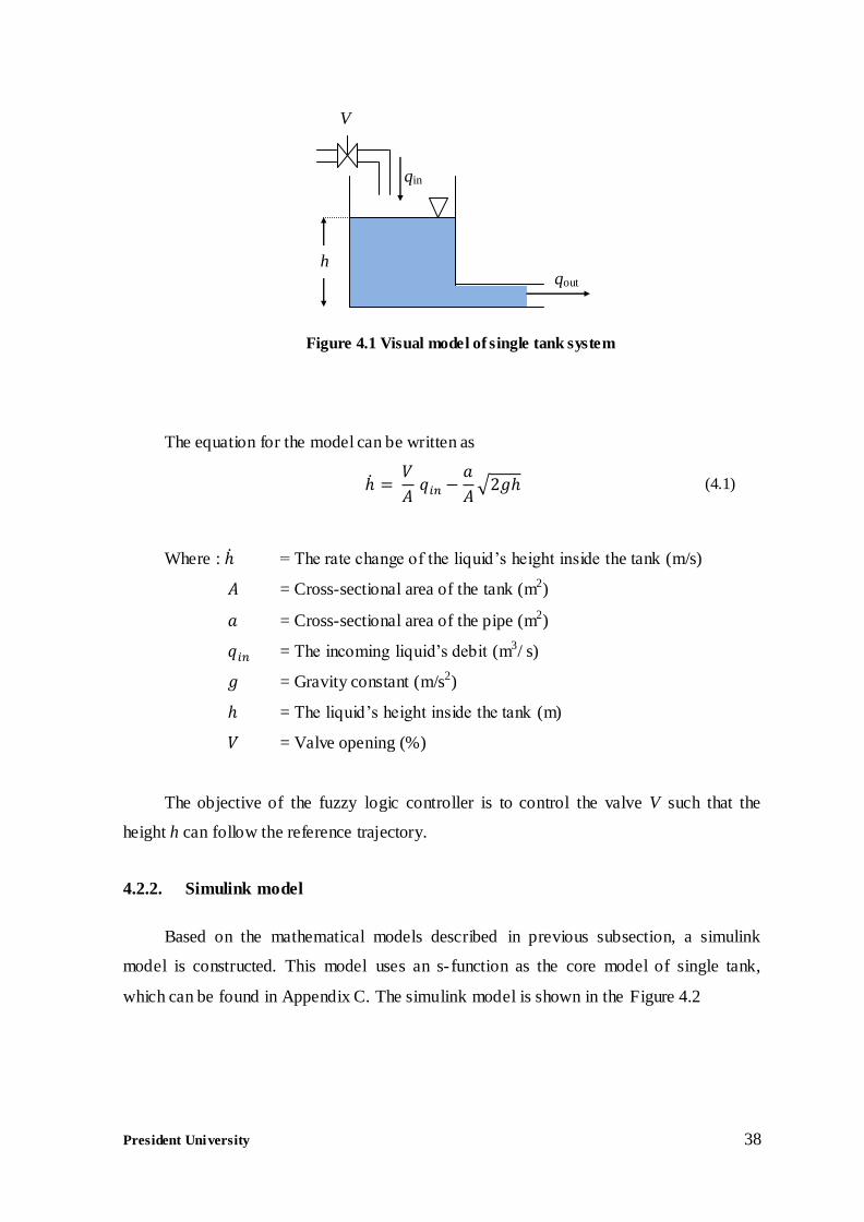
4.2.1. Mathematical Model of The System
Figure 4.1 shows the visual model of single tank system.
V1
President University 38
The equation for the model can be written as
(4.1)
Where : = The rate change of the liquid’s height inside the tank (m/s)
= Cross-sectional area of the tank (m2)
= Cross-sectional area of the pipe (m2)
= The incoming liquid’s debit (m3/ s)
= Gravity constant (m/s2)
= The liquid’s height inside the tank (m)
= Valve opening (%)
The objective of the fuzzy logic controller is to control the valve V such that the
height h can follow the reference trajectory.
4.2.2. Simulink model
Based on the mathematical models described in previous subsection, a simulink
model is constructed. This model uses an s- function as the core model of single tank,
which can be found in Appendix C. The simulink model is shown in the Figure 4.2
qin
h
qout
V
Figure 4.1 Visual model of single tank system
President University 39
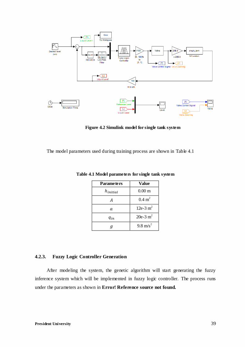
Figure 4.2 Simulink model for single tank system
The model parameters used during training process are shown in Table 4.1
Table 4.1 Model parameters for single tank system
Parameters Value
0.00 m
0.4 m2
12e-3 m2
20e-3 m2
9.8 m/s2
4.2.3. Fuzzy Logic Controller Generation
After modeling the system, the genetic algorithm will start generating the fuzzy
inference system which will be implemented in fuzzy logic controller. The process runs
under the parameters as shown in Error! Reference source not found.
President University 40
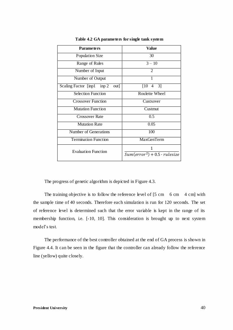
Table 4.2 GA parameters for single tank system
Parameters Value
Population Size 30
Range of Rules 3 – 10
Number of Input 2
Number of Output 1
Scaling Factor [inp1 inp 2 out] [10 4 3]
Selection Function Roulette Wheel
Crossover Function Custxover
Mutation Function Custmut
Crossover Rate 0.5
Mutation Rate 0.05
Number of Generations 100
Termination Function MaxGenTerm
Evaluation Function
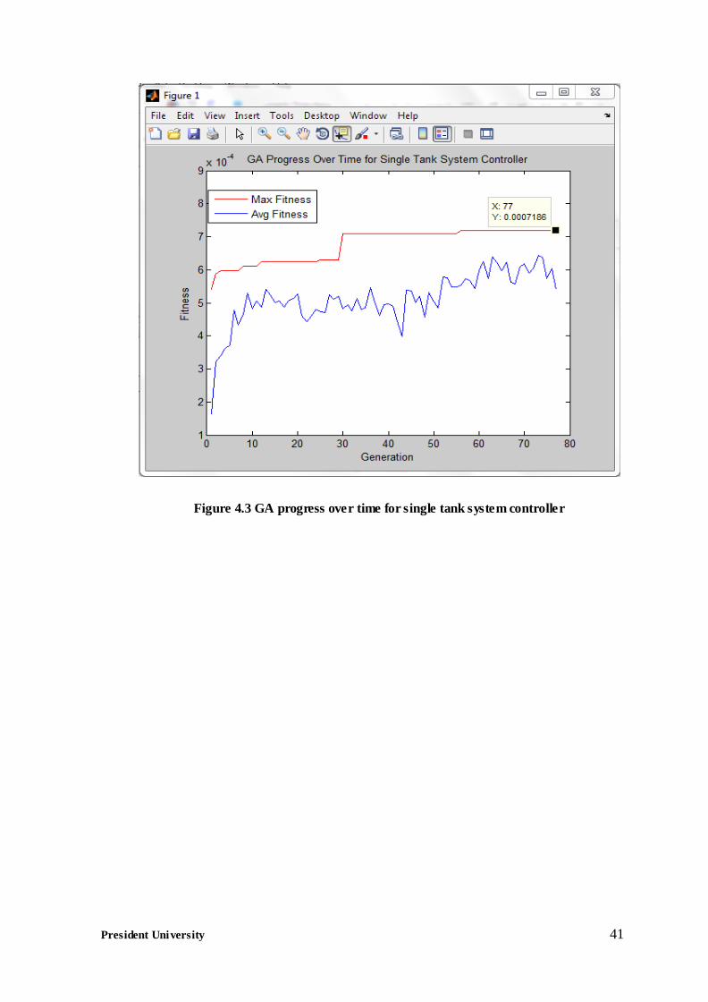
The progress of genetic algorithm is depicted in Figure 4.3.
The training objective is to follow the reference level of [5 cm 6 cm 4 cm] with
the sample time of 40 seconds. Therefore each simulation is run for 120 seconds. The set
of reference level is determined such that the error variable is kept in the range of its
membership function, i.e. [-10, 10]. This consideration is brought up to next system
model’s test.
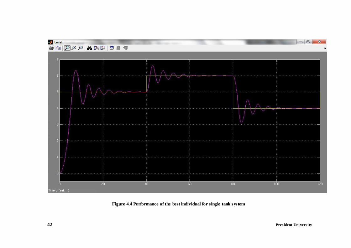
The performance of the best controller obtained at the end of GA process is shown in
Figure 4.4. It can be seen in the figure that the controller can already follow the reference
line (yellow) quite closely.
President University 41
Figure 4.3 GA progress over time for single tank system controller
42 President University
Figure 4.4 Performance of the best individual for single tank system

President University 43
4.2.4. Controller Test.
Further test is conducted in order to make sure that the controller works properly not
only in the universe of training set. Therefore, the controller is tested in three different
initial conditions; 10 cm, 3 cm, and 15 cm.
The important thing should be noted in determining the new initial condition and the
reference for this system and also the later systems is to keep the error variable to be inside
the range of membership function, which lies in [-10,10] in this system. The reason behind
it is the error outside the range will be ignored by the controller, thus in many case the
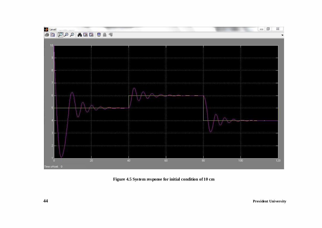
controller may not work properly. However, in the case of single tank system, setting
initial error much higher than the range might work since by not doing anything, the liquid
inside the tank will be drained automatically (see Figure 4.1) until the error falls inside the
appropriate range. This is, of course, not good to test the controller. By taking this
consideration, the initial conditions are set as mentioned above and the tests are conducted.
The results can be seen in Figure 4.5, Figure 4.6, and Figure 4.7.
44 President University
Figure 4.5 System response for initial condition of 10 cm
45 President University
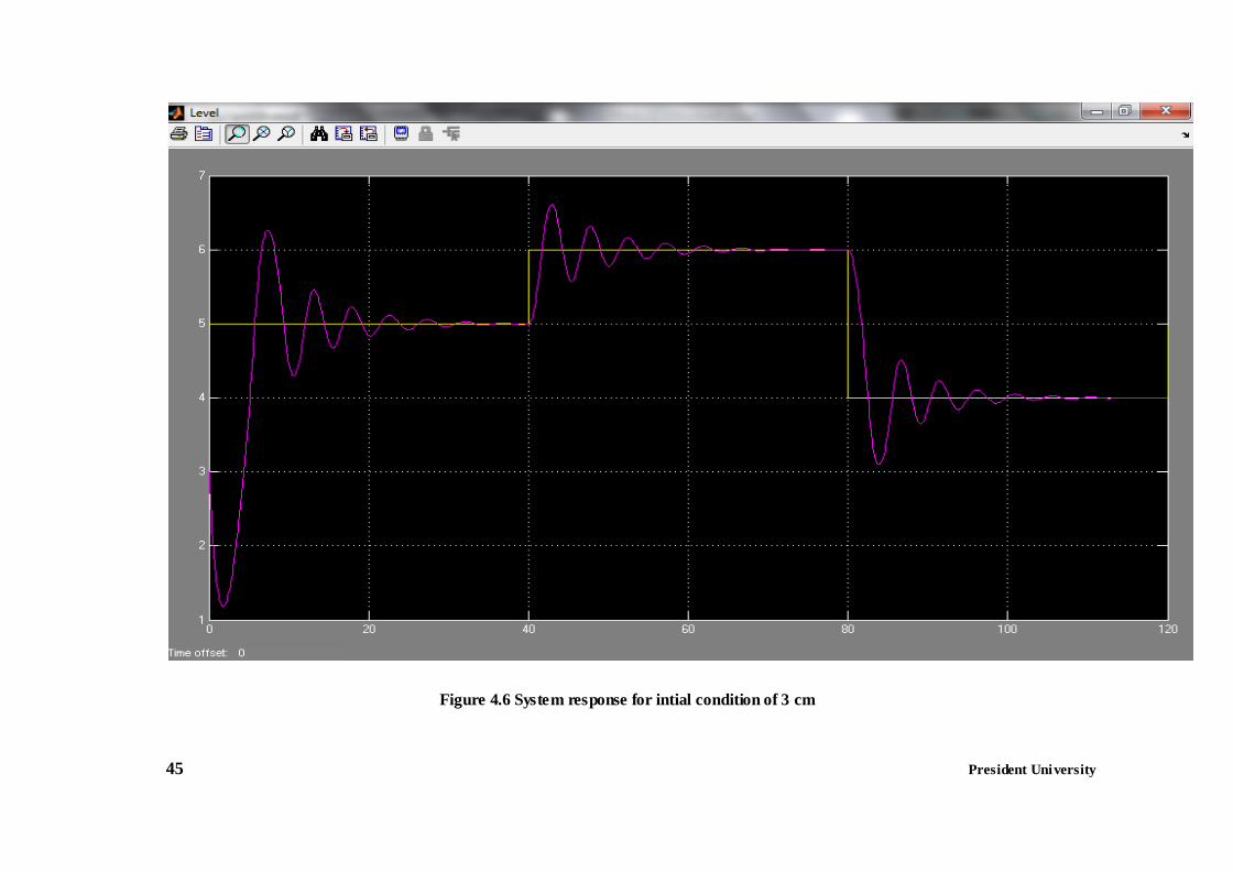
Figure 4.6 System response for intial condition of 3 cm
46 President University
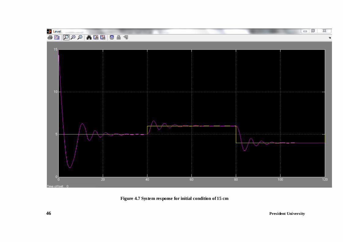
Figure 4.7 System response for initial condition of 15 cm
President University 47 President University
From the figures above, we can see that although the controller is still imperfect (the
liquid’s height must fall below 5 cm first before reaching 5 cm), it can follows the
reference closely.
4.3. Training and Test for Interacting Tank System
4.3.1. Mathematical model of the system
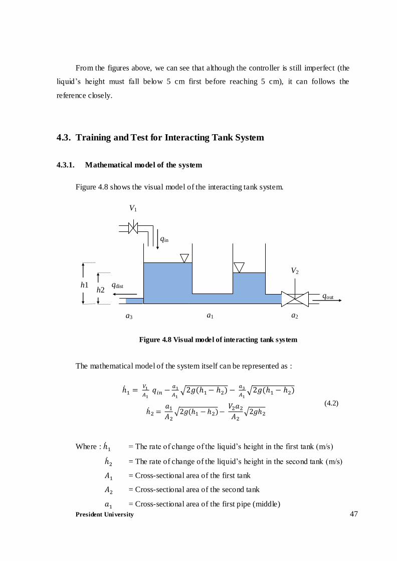
Figure 4.8 shows the visual model of the interacting tank system.
The mathematical model of the system itself can be represented as :
(4.2)
Where : = The rate of change of the liquid’s height in the first tank (m/s)
= The rate of change of the liquid’s height in the second tank (m/s)
= Cross-sectional area of the first tank
= Cross-sectional area of the second tank
= Cross-sectional area of the first pipe (middle)
Figure 4.8 Visual model of interacting tank system
V1
qin
h1
qout
V2
qdist h2
a
1
a
2
a
3
V1
V2
a1 a2 a3
President University 48 President University
= Cross-sectional area of the second pipe (right)
= Cross-sectional area of the third pipe (left)
= The incoming liquid’s debit (m3/ s)
= Gravity constant (m/s2)
= The liquid’s height inside the first tank (m)
= The liquid’s height inside the second tank (m)
= The opening of valve 1 (%)
= The opening of valve 2 (%)
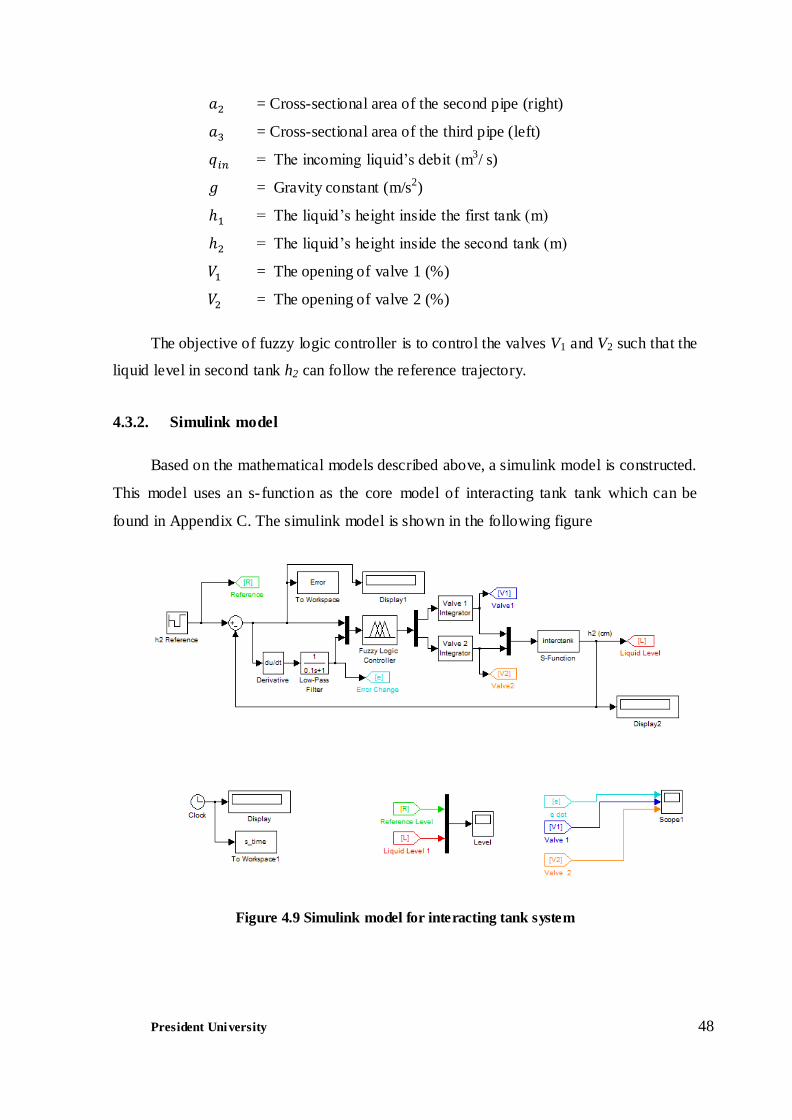
The objective of fuzzy logic controller is to control the valves V1 and V2 such that the
liquid level in second tank h2 can follow the reference trajectory.
4.3.2. Simulink model
Based on the mathematical models described above, a simulink model is constructed.
This model uses an s- function as the core model of interacting tank tank which can be
found in Appendix C. The simulink model is shown in the following figure
Figure 4.9 Simulink model for interacting tank system
President University 49 President University
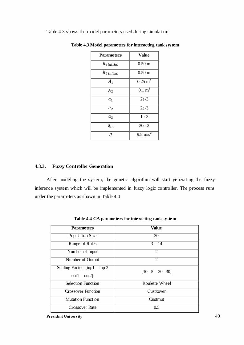
Table 4.3 shows the model parameters used during simulation
Table 4.3 Model parameters for interacting tank system
Parameters Value
0.50 m
0.50 m
0.25 m2
0.1 m2
2e-3
2e-3
1e-3
20e-3
9.8 m/s2
4.3.3. Fuzzy Controller Generation
After modeling the system, the genetic algorithm will start generating the fuzzy
inference system which will be implemented in fuzzy logic controller. The process runs
under the parameters as shown in Table 4.4
Table 4.4 GA parameters for interacting tank system
Parameters Value
Population Size 30
Range of Rules 3 – 14
Number of Input 2
Number of Output 2
Scaling Factor [inp1 inp 2
out1 out2] [10 5 30 30]
Selection Function Roulette Wheel
Crossover Function Custxover
Mutation Function Custmut
Crossover Rate 0.5
President University 50 President University
Mutation Rate 0.05
Number of Generations 100
Termination Function MaxGenTerm
Evaluation Function
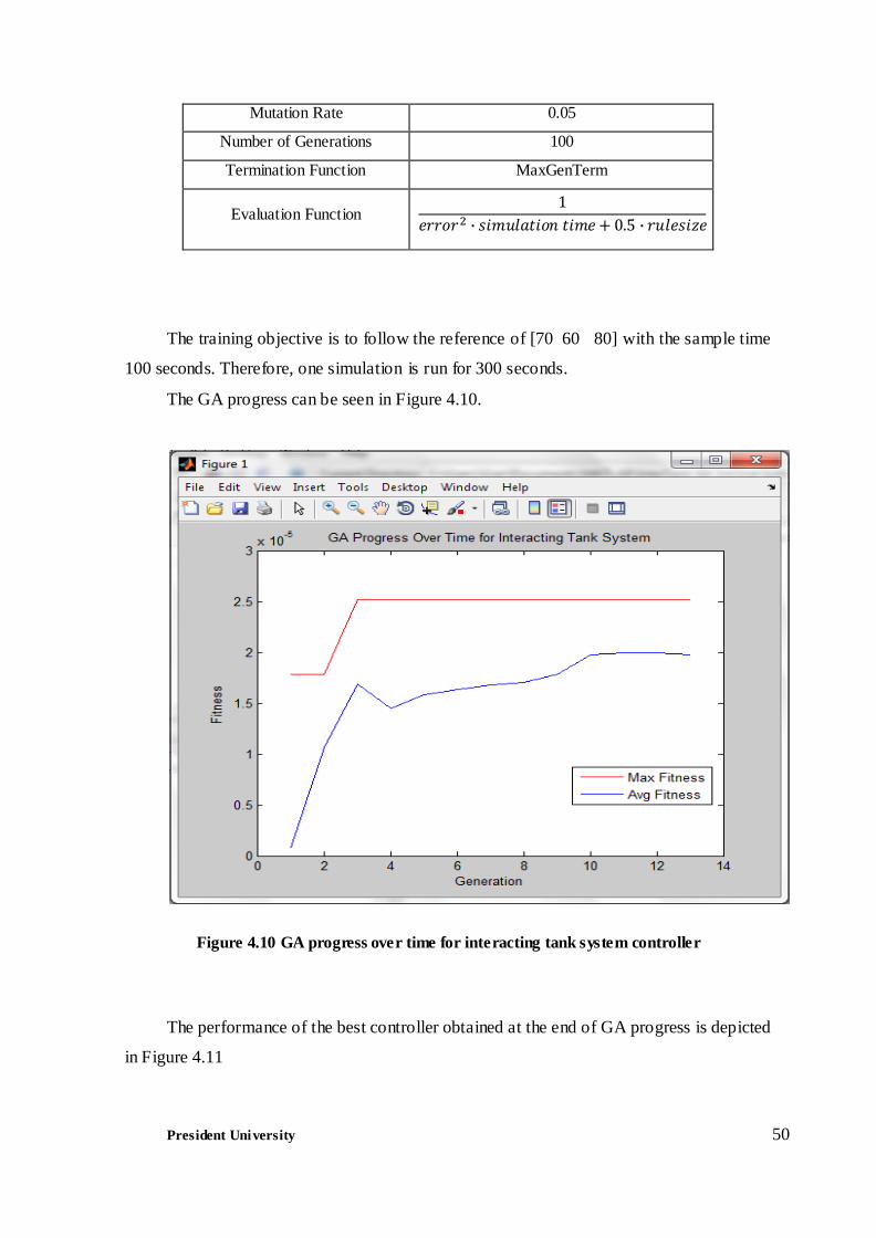
The training objective is to follow the reference of [70 60 80] with the sample time
100 seconds. Therefore, one simulation is run for 300 seconds.
The GA progress can be seen in Figure 4.10.
Figure 4.10 GA progress over time for interacting tank system controller
The performance of the best controller obtained at the end of GA progress is depicted
in Figure 4.11
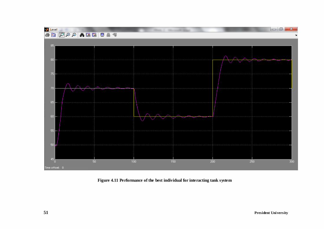
51 President University
Figure 4.11 Performance of the best individual for interacting tank system

President University 52 President University President University
4.3.4. Controller Test
Similar to single tank system, a series of tests are employed to make sure that the
controller can work under initial conditions different from the ones in training s et. A
consideration of variable range should also be taken into account. The sets of new initial
conditions are 60 cm, 80 cm, and 90 cm for both tanks. The purpose of this setup is to
check if the method of creating mirror image (section 3.2.3) really works. The results can
be seen in Figure 4.12, Figure 4.13, and Figure 4.14.
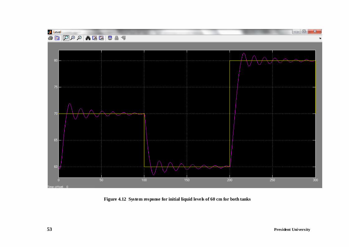
53 President University
Figure 4.12 System response for initial liquid levels of 60 cm for both tanks
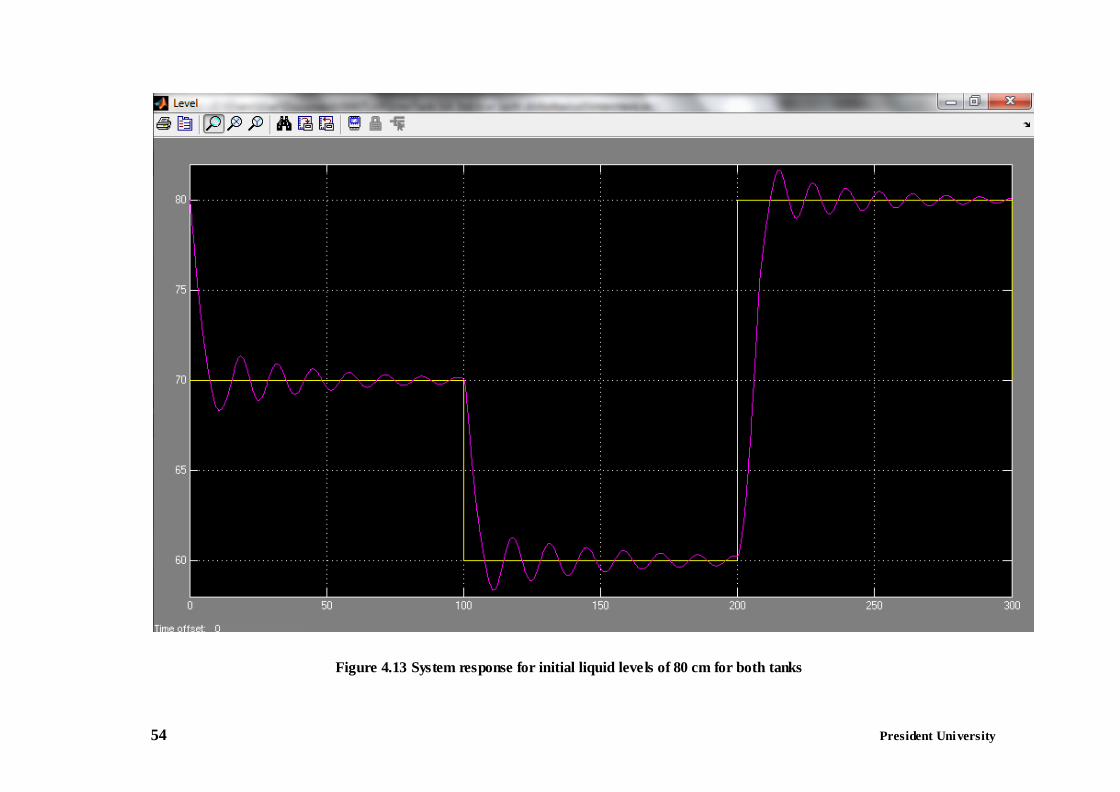
54 President University
Figure 4.13 System response for initial liquid levels of 80 cm for both tanks
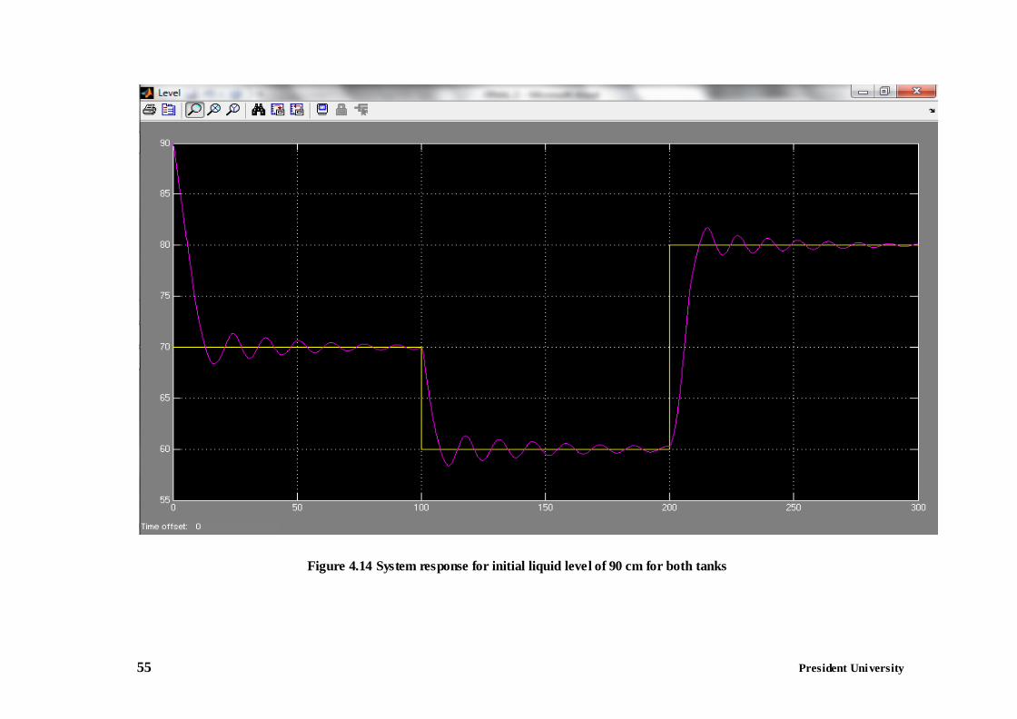
55 President University
Figure 4.14 System response for initial liquid level of 90 cm for both tanks
President University 56
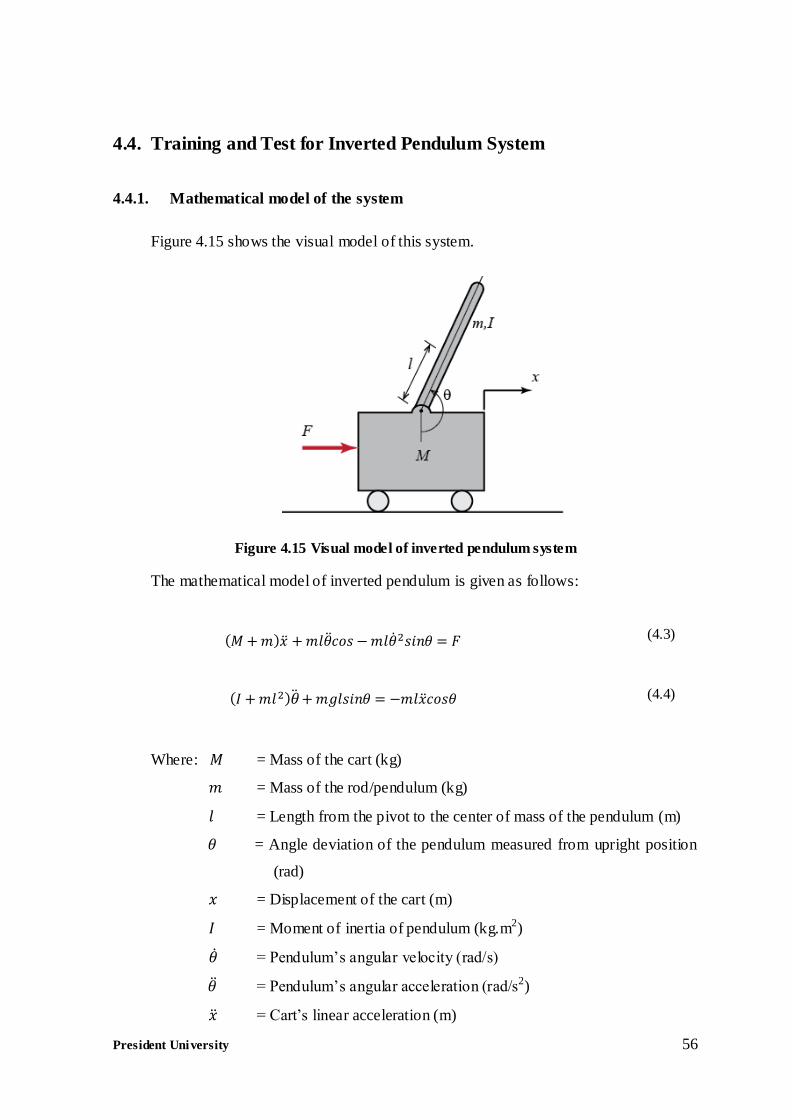
4.4. Training and Test for Inverted Pendulum System
4.4.1. Mathematical model of the system
Figure 4.15 shows the visual model of this system.
Figure 4.15 Visual model of inverted pendulum system
The mathematical model of inverted pendulum is given as follows:
(4.3)
(4.4)
Where: = Mass of the cart (kg)
= Mass of the rod/pendulum (kg)
= Length from the pivot to the center of mass of the pendulum (m)
= Angle deviation of the pendulum measured from upright position
(rad)
= Displacement of the cart (m)
= Moment of inertia of pendulum (kg.m2)
= Pendulum’s angular velocity (rad/s)
= Pendulum’s angular acceleration (rad/s2)
= Cart’s linear acceleration (m)

President University 57
= Force applied to the cart (kg.m2)
4.4.2. Simulink modeling
This time, due to the short simulation time, the usage of an s- function is unnecessary.
Thus, everything is modeled by using simulink’s blocks.
Figure 4.16 shows the inverted pendulum system model.
Figure 4.16 Simulink model for inverted pendulum system
Notice that there is a stop block in this model. This stop block is used to terminate
the simulation immediately if a certain condition, declared in the function block before it,
is fulfilled. The function block right before stop block check if the value of θ is greater
than or equal to 90 degree. If so, then the simulation is terminated.
Another block also appears replacing the place where the s- function is used to be.
This is the cart & pole dynamics subsystem block which contains the model of the inverted
pendulum. Figure 4.17 shows the contents of this block.
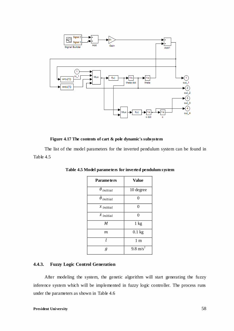
President University 58
Figure 4.17 The contents of cart & pole dynamic's subsystem
The list of the model parameters for the inverted pendulum system can be found in
Table 4.5
Table 4.5 Model parameters for inverted pendulum system
Parameters Value
10 degree
0
0
0
1 kg
0.1 kg
1 m
9.8 m/s2
4.4.3. Fuzzy Logic Control Generation
After modeling the system, the genetic algorithm will start generating the fuzzy
inference system which will be implemented in fuzzy logic controller. The process runs
under the parameters as shown in Table 4.6
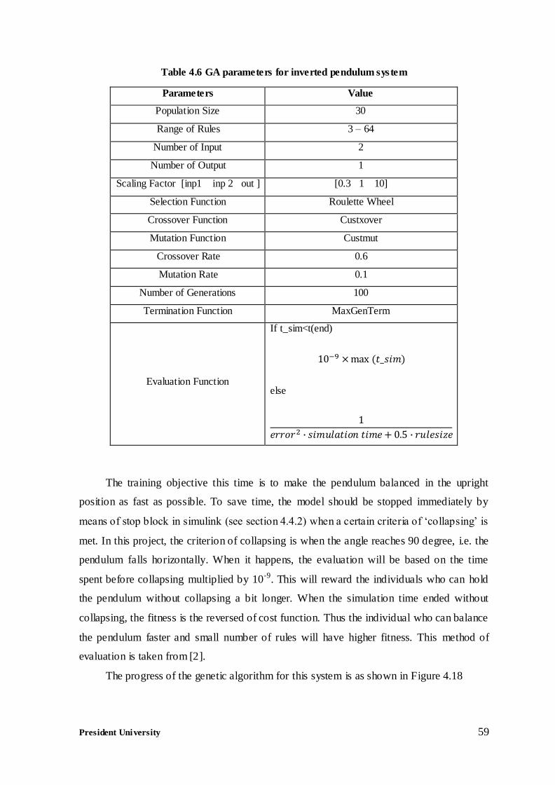
President University 59
Table 4.6 GA parameters for inverted pendulum system
Parameters Value
Population Size 30
Range of Rules 3 – 64
Number of Input 2
Number of Output 1
Scaling Factor [inp1 inp 2 out ] [0.3 1 10]
Selection Function Roulette Wheel
Crossover Function Custxover
Mutation Function Custmut
Crossover Rate 0.6
Mutation Rate 0.1
Number of Generations 100
Termination Function MaxGenTerm
Evaluation Function
If t_sim<t(end)
else
The training objective this time is to make the pendulum balanced in the upright
position as fast as possible. To save time, the model should be stopped immediately by
means of stop block in simulink (see section 4.4.2) when a certain criteria of ‘collapsing’ is
met. In this project, the criterion of collapsing is when the angle reaches 90 degree, i.e. the
pendulum falls horizontally. When it happens, the evaluation will be based on the time
spent before collapsing multiplied by 10-9. This will reward the individuals who can hold
the pendulum without collapsing a bit longer. When the simulation time ended without
collapsing, the fitness is the reversed of cost function. Thus the individual who can balance
the pendulum faster and small number of rules will have higher fitness. This method of
evaluation is taken from [2].
The progress of the genetic algorithm for this system is as shown in Figure 4.18
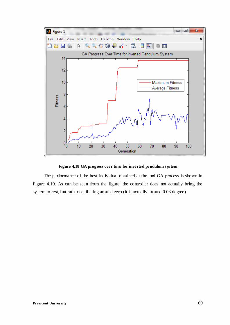
President University 60
Figure 4.18 GA progress over time for inverted pendulum sys tem
The performance of the best individual obtained at the end GA process is shown in
Figure 4.19. As can be seen from the figure, the controller does not actually bring the
system to rest, but rather oscillating around zero (it is actually around 0.03 degree).
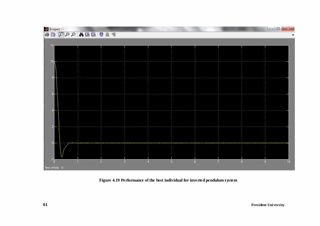
61 President University
Figure 4.19 Performance of the best individual for inverted pendulum system
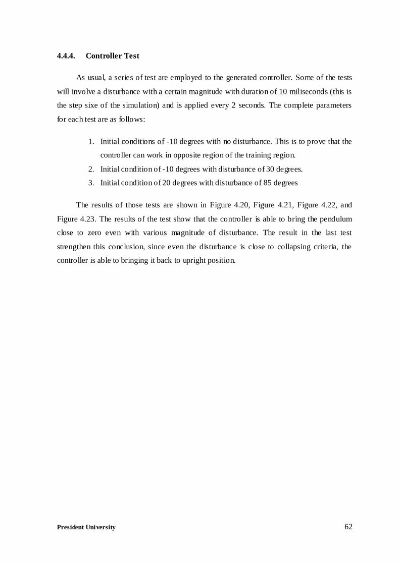
President University 62
4.4.4. Controller Test
As usual, a series of test are employed to the generated controller. Some of the tests
will involve a disturbance with a certain magnitude with duration of 10 miliseconds (this is
the step sixe of the simulation) and is applied every 2 seconds. The complete parameters
for each test are as follows:
1. Initial conditions of -10 degrees with no disturbance. This is to prove that the
controller can work in opposite region of the training region.
2. Initial condition of -10 degrees with disturbance of 30 degrees.
3. Initial condition of 20 degrees with disturbance of 85 degrees
The results of those tests are shown in Figure 4.20, Figure 4.21, Figure 4.22, and
Figure 4.23. The results of the test show that the controller is able to bring the pendulum
close to zero even with various magnitude of disturbance. The result in the last test
strengthen this conclusion, since even the disturbance is close to collapsing criteria, the
controller is able to bringing it back to upright position.
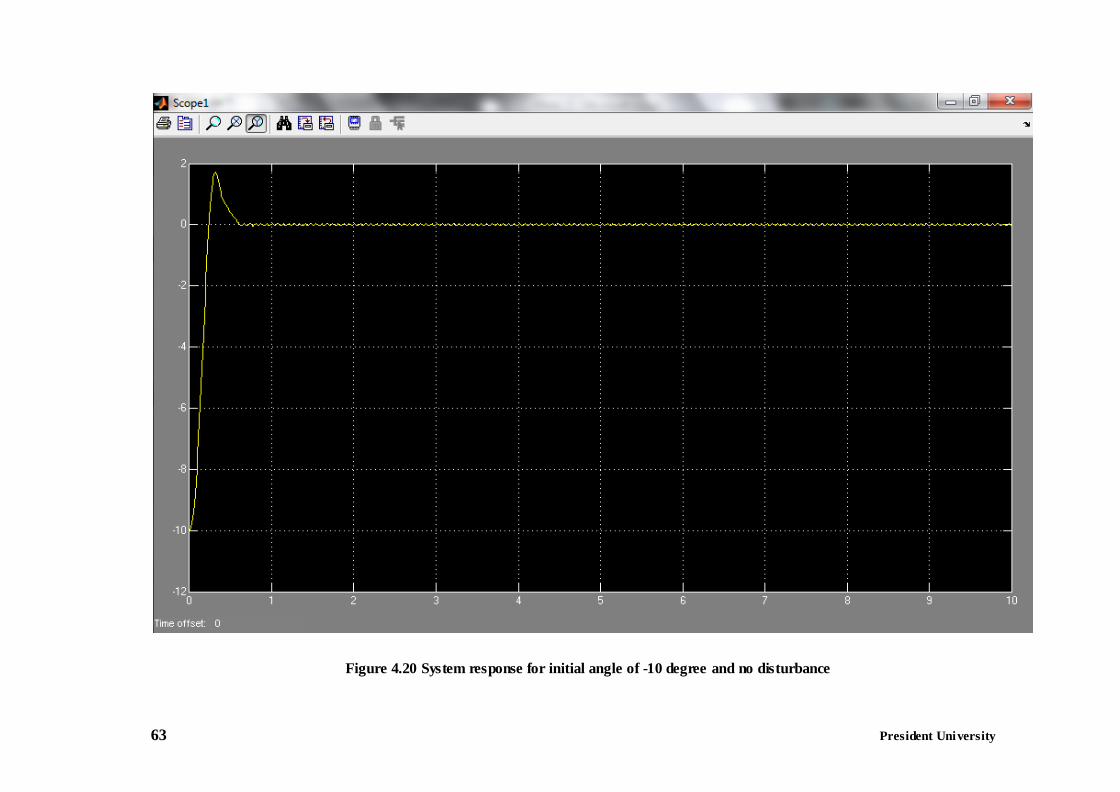
63 President University
Figure 4.20 System response for initial angle of -10 degree and no disturbance
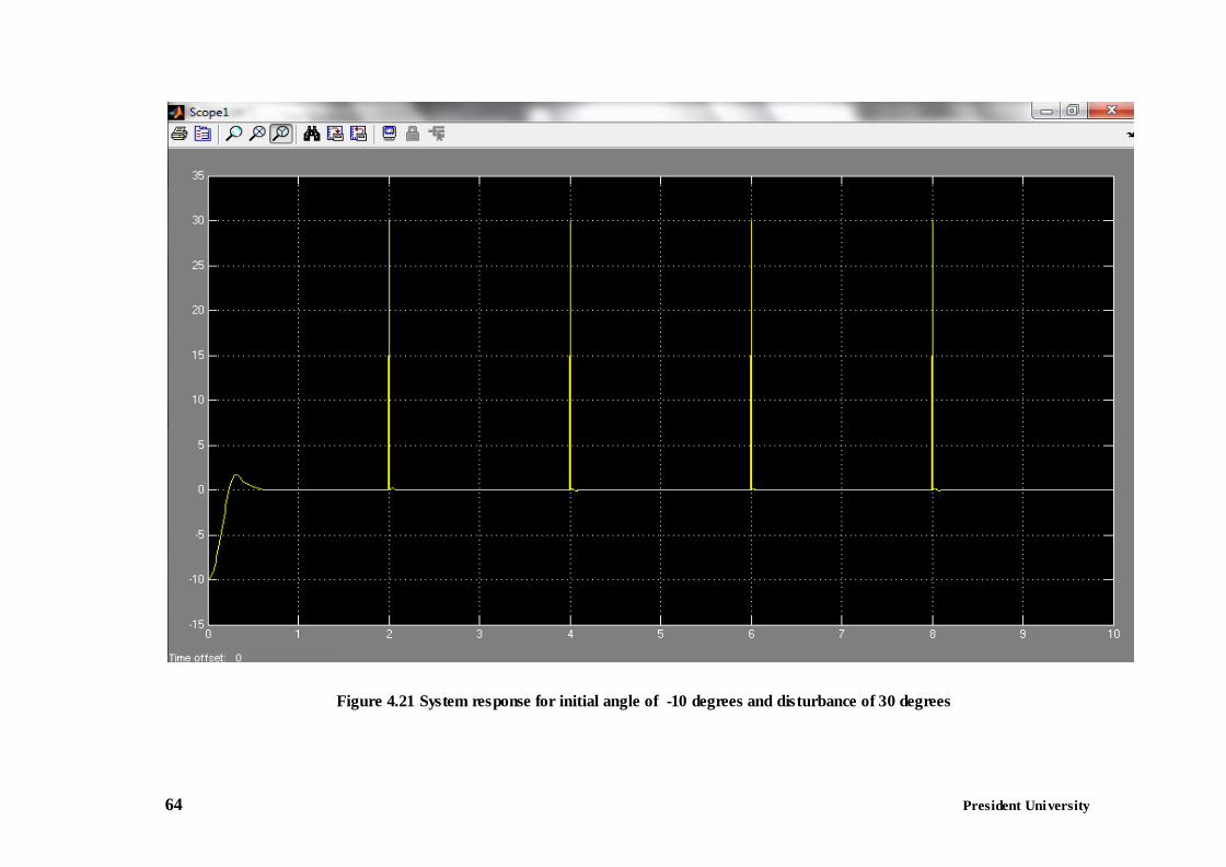
64 President University
Figure 4.21 System response for initial angle of -10 degrees and disturbance of 30 degrees
65 President University
Figure 4.22 System response for initial angle of 10 degrees and disturbance of 30 degrees
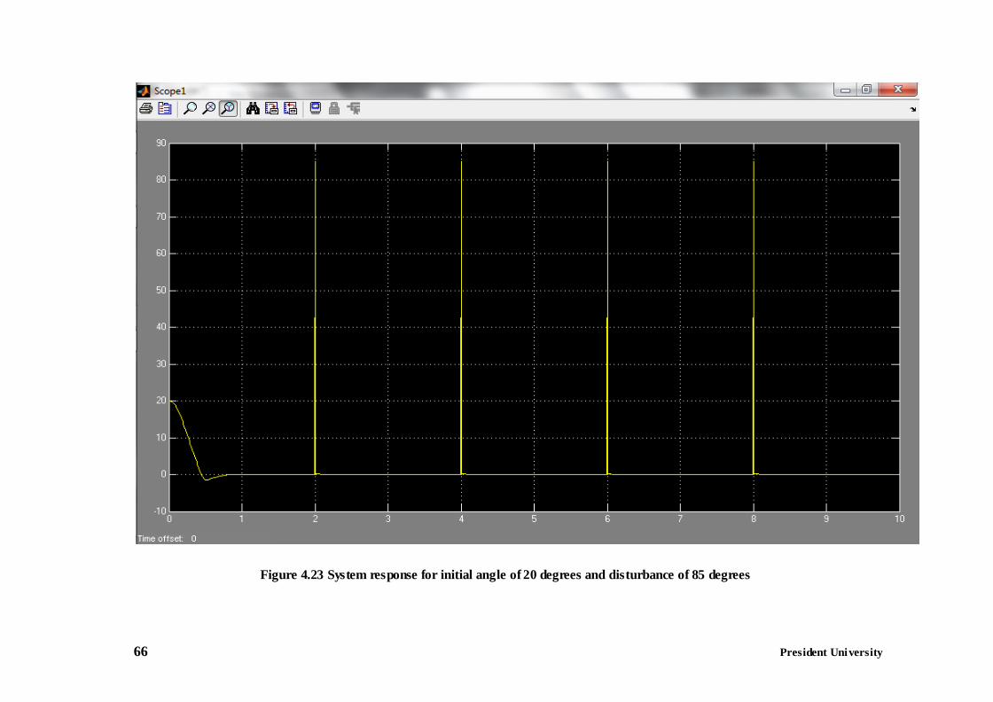
66 President University
Figure 4.23 System response for initial angle of 20 degrees and disturbance of 85 degrees
President University 67 President University
CHAPTER 5
CONCLUSION AND FUTURE WORKS
5.1. Conclusion
A method to auto-generate fuzzy logic controller has been developed in this project.
A modified genetic algorithm is integrated into the design process which will search for the
best combination of rules to be included in the rule base of fuzzy inference system.
The strengths of the method developed in this project are:
1) The ability to perform the generation and optimization process of data base and
rule base at once
2) The ability to preserve the genetic materials throughout the evolution process
3) The ability in filtering the unnecessary variables and the excessive rules
4) The ability to counter the problem of non-uniformity distribution of membership
which is caused by the random generation of rules parameters easily.
Several different models are also used to prove the generality and the effectiveness of
the method. This model includes the inverted pendulum model, which is commonly used
as a benchmark to test the new method to generate fuzzy logic controller, and the result is
also satisfactory.
Despite of several successful tests in this project, there are still many rooms for
improvement of the method. Therefore, a further investigation to improve it is highly
encouraged.
5.2. Future Works
There are several aspects which can be done to improve the method presented in this
final project:

President University 68 President University
1. The further investigation in varying the GA parameters is highly encouraged. Due to
the time constraint, this project uses the same parameters for almost every model.
There is a high possibility that usage of other variation of parameters will improve
the result.
2. For the sake of simplicity, this project uses default setting of membership function
with isosceles triangular membership function. Further research might be conducted
to investigate the effect in changing these aspects, for example changing the
triangular membership function to gaussian, changing Mamdani type FIS to be
Sugeno type, etc.
President University 69 President University
BIBLIOGRAPHY
[1] Cordón, Oscar, Herrera, Francisco, Hoffman, Frank, and Magdalena, Luis,
“Genetic Fuzzy Systems: Evolutionary Tuning and Learning of Fuzzy Knowledge
Bases,” Advances in Fuzzy Systems – Applications and Theory Vol.19, World
Scientific Publishing Co. Pte. Ltd, 2001.
[2] Foran, Joseph, “Optimisation of a Fuzzy Logic Controller Using Genetic
Algorithms,” 2002.
[3] Cooper, G., Mark, and Vidal, J., Jacques, “Genetic Design of Fuzzy
Controller,” University of California, Los Angeles.
[4] Chen, Min-You, and Linkens, D.A., “Rule-Base Self-Generation and
Simplification for Data-Driven Fuzzy Models,” Elsevier, 2003.
[5] Sitompul, Erwin. Class Lecture, Topic : “Sistem Modelling and
Identification Lecture 6” Faculty of Engineering, Electrical Engineering Major,
President University, Cikarang, Indonesia, Oct. 16, 2011.
[6] The Mathwork, “Simulink: Model-Based and System-Based Design,” The
Mathwork, Inc., 2001.
[7] Sivanandam, S.N, Sumathi,S., and Deepa, S.N., “Introduction to Fuzzy
Logic using MATLAB,” Springer, 2007.
[8] Sivanandam, S.N, and Deepa, S.N., “Introduction to Genetic Algorithms,”
Springer, 2008.
[9] The MathWork, “Learning Matlab 7,” The Mathwork Inc., 2005.
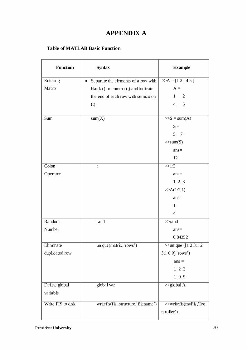
President University 70 President University
APPENDIX A
Table of MATLAB Basic Function
Function Syntax Example
Entering
Matrix
Separate the elements of a row with
blank () or comma (,) and indicate
the end of each row with semicolon
(;)
>>A = [1 2 ; 4 5 ]
A =
1 2
4 5
Sum sum(X) >>S = sum(A)
S =
5 7
>>sum(S)
ans=
12
Colon
Operator
: >>1:3
ans=
1 2 3
>>A(1:2,1)
ans=
1
4
Random
Number
rand >>rand
ans=
0.84352
Eliminate
duplicated row
unique(matrix,’rows’) >>unique ([1 2 3;1 2
3;1 0 9],’rows’)
ans =
1 2 3
1 0 9
Define global
variable
global var >>global A
Write FIS to disk writefis(fis_structure,’filename’) >>writefis(myFis,’Ico
ntroller’)
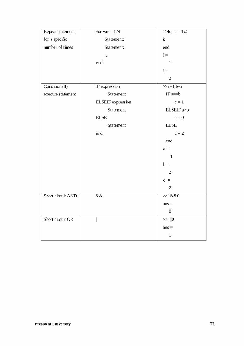
President University 71 President University
Repeat statements
for a specific
number of times
For var = 1:N
Statement;
Statement;
...
end
>>for i = 1:2
i;
end
i =
1
i =
2
Conditionally
execute statement
IF expression
Statement
ELSEIF expression
Statement
ELSE
Statement
end
>>a=1,b=2
IF a==b
c = 1
ELSEIF a>b
c = 0
ELSE
c = 2
end
a =
1
b =
2
c =
2
Short circuit AND && >>1&&0
ans =
0
Short circuit OR || >>1||0
ans =
1
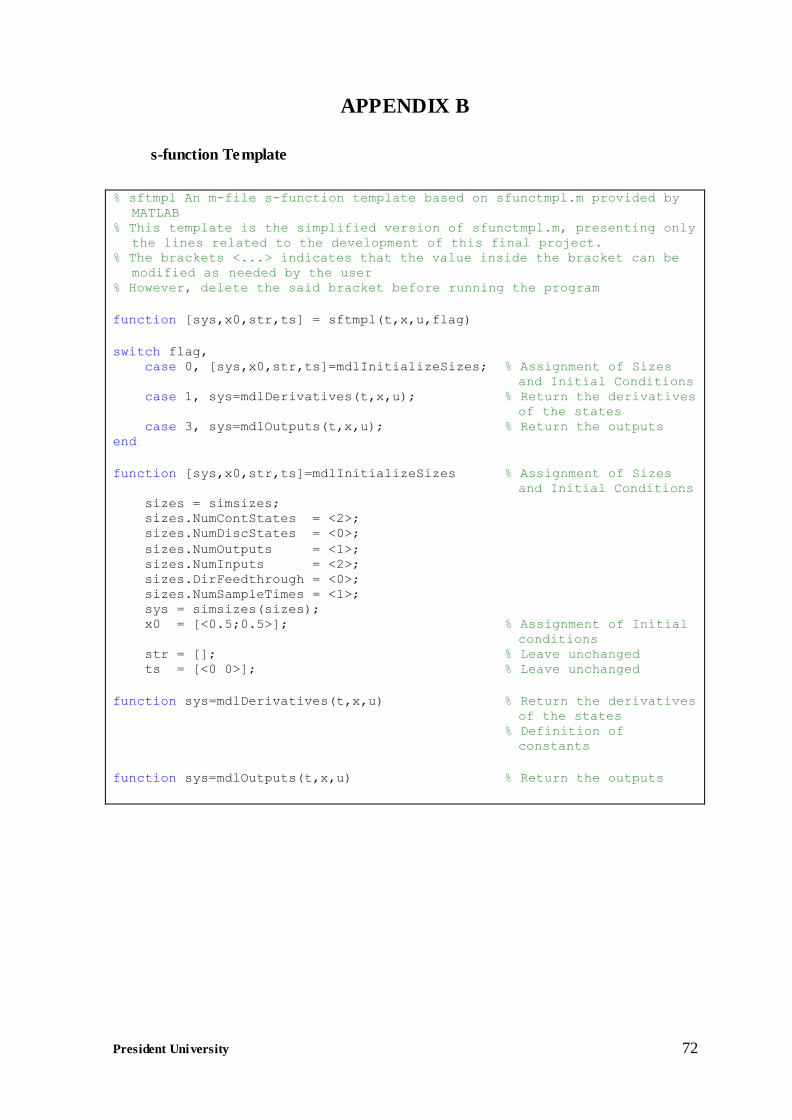
President University 72 President University
APPENDIX B
s-function Template
% sftmpl An m-file s-function template based on sfunctmpl.m provided by
MATLAB % This template is the simplified version of sfunctmpl.m, presenting only
the lines related to the development of this final project. % The brackets <...> indicates that the value inside the bracket can be
modified as needed by the user
% However, delete the said bracket before running the program
function [sys,x0,str,ts] = sftmpl(t,x,u,flag)
switch flag, case 0, [sys,x0,str,ts]=mdlInitializeSizes; % Assignment of Sizes
and Initial Conditions
case 1, sys=mdlDerivatives(t,x,u); % Return the derivatives
of the states
case 3, sys=mdlOutputs(t,x,u); % Return the outputs end
function [sys,x0,str,ts]=mdlInitializeSizes % Assignment of Sizes
and Initial Conditions
sizes = simsizes; sizes.NumContStates = <2>; sizes.NumDiscStates = <0>;
sizes.NumOutputs = <1>; sizes.NumInputs = <2>;
sizes.DirFeedthrough = <0>; sizes.NumSampleTimes = <1>; sys = simsizes(sizes);
x0 = [<0.5;0.5>]; % Assignment of Initial
conditions
str = []; % Leave unchanged ts = [<0 0>]; % Leave unchanged
function sys=mdlDerivatives(t,x,u) % Return the derivatives
of the states
% Definition of
constants
function sys=mdlOutputs(t,x,u) % Return the outputs
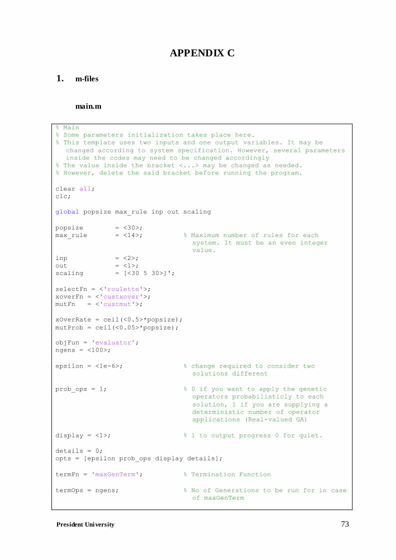
President University 73 President University
APPENDIX C
1. m-files
main.m
% Main % Some parameters initialization takes place here.
% This template uses two inputs and one output variables. It may be
changed according to system specification. However, several parameters
inside the codes may need to be changed accordingly % The value inside the bracket <...> may be changed as needed.
% However, delete the said bracket before running the program.
clear all;
clc;
global popsize max_rule inp out scaling
popsize = <30>;
max_rule = <14>; % Maximum number of rules for each
system. It must be an even integer
value.
inp = <2>; out = <1>;
scaling = [<30 5 30>]';
selectFn = <'roulette'>; xoverFn = <'custxover'>; mutFn = <'custmut'>;
xOverRate = ceil(<0.5>*popsize);
mutProb = ceil(<0.05>*popsize);
objFun = 'evaluator';
ngens = <100>;
epsilon = <1e-6>; % change required to consider two
solutions different
prob_ops = 1; % 0 if you want to apply the genetic
operators probabilisticly to each
solution, 1 if you are supplying a
deterministic number of operator
applications (Real-valued GA)
display = <1>; % 1 to output progress 0 for quiet.
details = 0;
opts = [epsilon prob_ops display details];
termFn = 'maxGenTerm'; % Termination Function
termOps = ngens; % No of Generations to be run for in case
of maxGenTerm
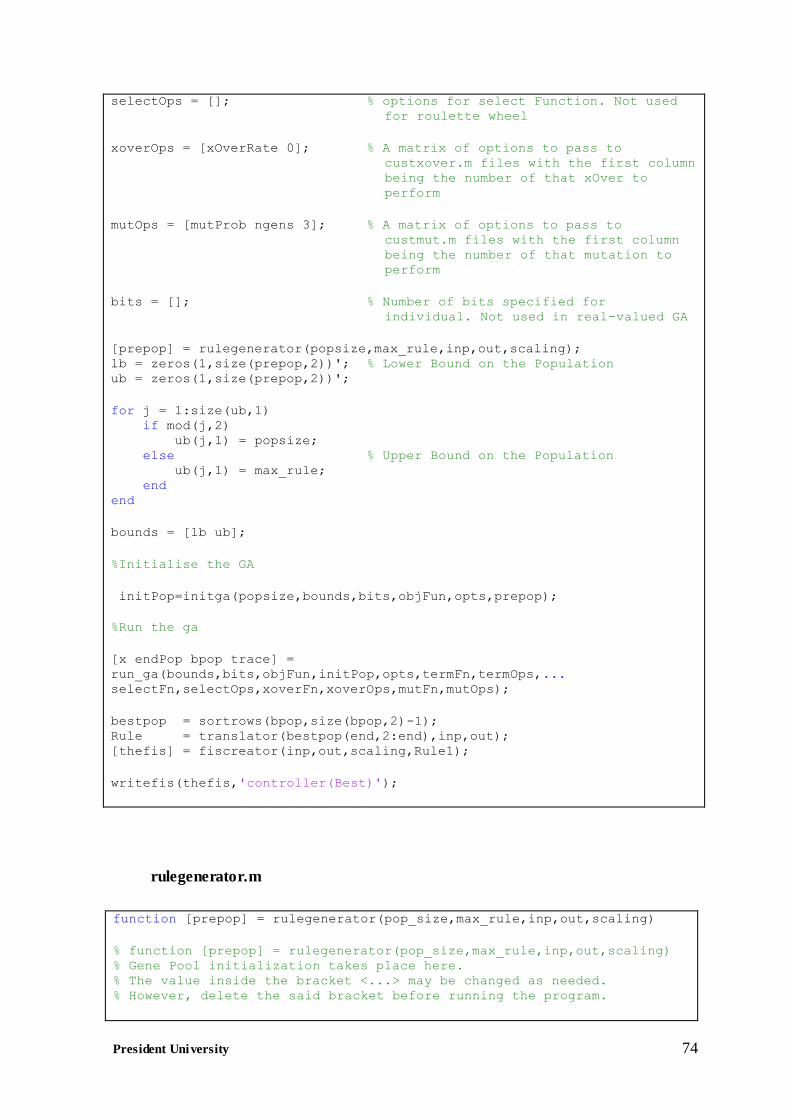
President University 74 President University
selectOps = []; % options for select Function. Not used
for roulette wheel
xoverOps = [xOverRate 0]; % A matrix of options to pass to
custxover.m files with the first column
being the number of that xOver to
perform
mutOps = [mutProb ngens 3]; % A matrix of options to pass to
custmut.m files with the first column
being the number of that mutation to
perform
bits = []; % Number of bits specified for
individual. Not used in real-valued GA
[prepop] = rulegenerator(popsize,max_rule,inp,out,scaling);
lb = zeros(1,size(prepop,2))'; % Lower Bound on the Population ub = zeros(1,size(prepop,2))';
for j = 1:size(ub,1)
if mod(j,2) ub(j,1) = popsize; else % Upper Bound on the Population
ub(j,1) = max_rule; end
end
bounds = [lb ub];
%Initialise the GA
initPop=initga(popsize,bounds,bits,objFun,opts,prepop);
%Run the ga
[x endPop bpop trace] =
run_ga(bounds,bits,objFun,initPop,opts,termFn,termOps,...
selectFn,selectOps,xoverFn,xoverOps,mutFn,mutOps);
bestpop = sortrows(bpop,size(bpop,2)-1);
Rule = translator(bestpop(end,2:end),inp,out); [thefis] = fiscreator(inp,out,scaling,Rule1);
writefis(thefis,'controller(Best)');
rulegenerator.m
function [prepop] = rulegenerator(pop_size,max_rule,inp,out,scaling)
% function [prepop] = rulegenerator(pop_size,max_rule,inp,out,scaling)
% Gene Pool initialization takes place here. % The value inside the bracket <...> may be changed as needed.
% However, delete the said bracket before running the program.
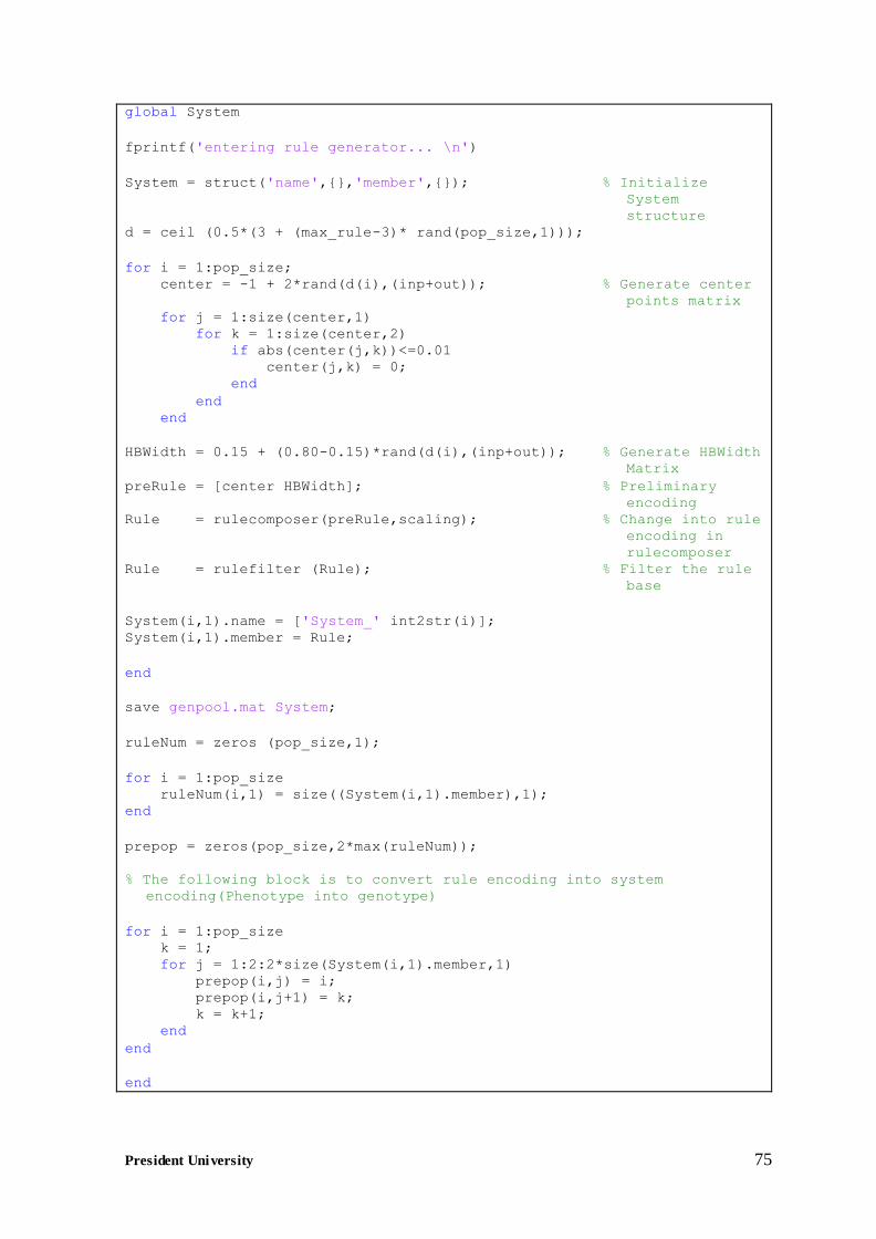
President University 75 President University
global System
fprintf('entering rule generator... \n')
System = struct('name',{},'member',{}); % Initialize
System
structure
d = ceil (0.5*(3 + (max_rule-3)* rand(pop_size,1)));
for i = 1:pop_size;
center = -1 + 2*rand(d(i),(inp+out)); % Generate center
points matrix
for j = 1:size(center,1) for k = 1:size(center,2)
if abs(center(j,k))<=0.01 center(j,k) = 0; end
end end
HBWidth = 0.15 + (0.80-0.15)*rand(d(i),(inp+out)); % Generate HBWidth
Matrix
preRule = [center HBWidth]; % Preliminary
encoding
Rule = rulecomposer(preRule,scaling); % Change into rule
encoding in
rulecomposer Rule = rulefilter (Rule); % Filter the rule
base
System(i,1).name = ['System_' int2str(i)];
System(i,1).member = Rule;
end
save genpool.mat System;
ruleNum = zeros (pop_size,1);
for i = 1:pop_size ruleNum(i,1) = size((System(i,1).member),1);
end
prepop = zeros(pop_size,2*max(ruleNum));
% The following block is to convert rule encoding into system
encoding(Phenotype into genotype)
for i = 1:pop_size k = 1; for j = 1:2:2*size(System(i,1).member,1)
prepop(i,j) = i; prepop(i,j+1) = k;
k = k+1; end
end
end
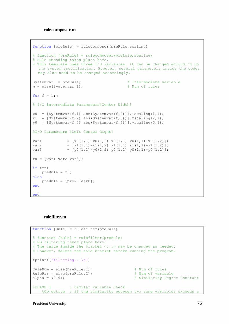
President University 76 President University
rulecomposer.m
function [preRule] = rulecomposer(preRule,scaling)
% function [preRule] = rulecomposer(preRule,scaling)
% Rule Encoding takes place here. % This template uses three I/O variables. It can be changed according to
the system specification. However, several parameters inside the codes
may also need to be changed accordingly.
Systemvar = preRule; % Intermediate variable m = size(Systemvar,1); % Num of rules
for f = 1:m
% I/O intermediate Parameters[Center Width]
x0 = [Systemvar(f,1) abs(Systemvar(f,4))].*scaling(1,1); x1 = [Systemvar(f,2) abs(Systemvar(f,5))].*scaling(2,1); y0 = [Systemvar(f,3) abs(Systemvar(f,6))].*scaling(3,1);
%I/O Parameters [Left Center Right]
var1 = [x0(1,1)-x0(1,2) x0(1,1) x0(1,1)+x0(1,2)];
var2 = [x1(1,1)-x1(1,2) x1(1,1) x1(1,1)+x1(1,2)]; var3 = [y0(1,1)-y0(1,2) y0(1,1) y0(1,1)+y0(1,2)];
r0 = [var1 var2 var3];
if f==1 preRule = r0;
else
preRule = [preRule;r0]; end
end
rulefilter.m
function [Rule] = rulefilter(preRule)
% function [Rule] = rulefilter(preRule)
% RB filtering takes place here. % The value inside the bracket <...> may be changed as needed.
% However, delete the said bracket before running the program.
fprintf('filtering...\n')
RuleNum = size(preRule,1); % Num of rules RulePar = size(preRule,2); % Num of variable
alpha = <0.9>; % Similarity Degree Constant
%PHASE 1 : Similar variable Check %Objective : if the similarity between two same variables exceeds a
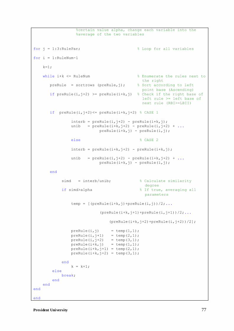
President University 77 President University
%certain value alpha, change each variable into the %average of the two variables
for j = 1:3:RulePar; % Loop for all variables
for i = 1:RuleNum-1
k=1;
while i+k <= RuleNum % Enumerate the rules next to
the right
preRule = sortrows (preRule,j); % Sort according to left
point base (Ascending)
if preRule(i,j+2) >= preRule(i+k,j) % Check if the right base of
left rule >= left base of
next rule (RBI>=LBII)
if preRule(i,j+2)<= preRule(i+k,j+2) % CASE 1
interb = preRule(i,j+2) - preRule(i+k,j);
unib = preRule(i+k,j+2) - preRule(i,j+2) + ...
preRule(i+k,j) - preRule(i,j);
else % CASE 2
interb = preRule(i+k,j+2) - preRule(i+k,j);
unib = preRule(i,j+2) - preRule(i+k,j+2) + ...
preRule(i+k,j) - preRule(i,j);
end
simd = interb/unib; % Calculate similarity
degree if simd>alpha % If true, averaging all
parameters
temp = [(preRule(i+k,j)+preRule(i,j))/2;...
(preRule(i+k,j+1)+preRule(i,j+1))/2;...
(preRule(i+k,j+2)+preRule(i,j+2))/2];
preRule(i,j) = temp(1,1);
preRule(i,j+1) = temp(2,1);
preRule(i,j+2) = temp(3,1); preRule(i+k,j) = temp(1,1);
preRule(i+k,j+1) = temp(2,1); preRule(i+k,j+2) = temp(3,1);
end k = k+1;
else break;
end end end
end
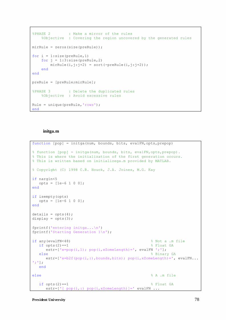
President University 78 President University
%PHASE 2 : Make a mirror of the rules
%Objective : Covering the region uncovered by the generated rules
mirRule = zeros(size(preRule));
for i = 1:size(preRule,1)
for j = 1:3:size(preRule,2)
mirRule(i,j:j+2) = sort(-preRule(i,j:j+2));
end end
preRule = [preRule;mirRule];
%PHASE 3 : Delete the duplicated rules %Objective : Avoid excessive rules
Rule = unique(preRule,'rows'); end
initga.m
function [pop] = initga(num, bounds, bits, evalFN,opts,prepop)
% function [pop] = initga(num, bounds, bits, evalFN,opts,prepop).
% This is where the initialization of the first generation occurs. % This is written based on initializega.m provided by MATLAB.
% Copyright (C) 1998 C.R. Houck, J.A. Joines, M.G. Kay
if nargin<5 opts = [1e-6 1 0 0];
end
if isempty(opts) opts = [1e-6 1 0 0]; end
details = opts(4);
display = opts(3);
fprintf('entering initga...\n')
fprintf('Starting Generation 1\n');
if any(evalFN<48) % Not a .m file if opts(2)==1 % Float GA
estr=['x=pop(i,1); pop(i,xZomeLength)=', evalFN ';']; else % Binary GA estr=['x=b2f(pop(i,:),bounds,bits); pop(i,xZomeLength)=', evalFN...
';']; end
else % A .m file
if opts(2)==1 % Float GA estr=['[ pop(i,:) pop(i,xZomeLength)]=' evalFN ...
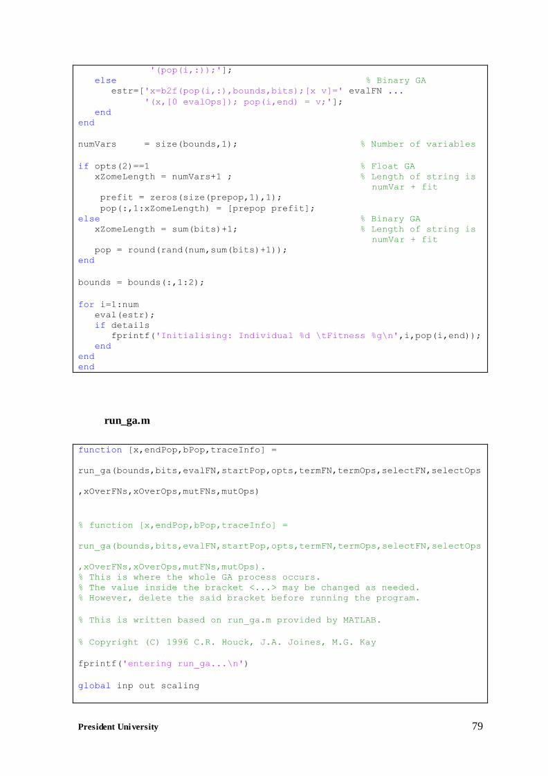
President University 79 President University
'(pop(i,:));'];
else % Binary GA
estr=['x=b2f(pop(i,:),bounds,bits);[x v]=' evalFN ...
'(x,[0 evalOps]); pop(i,end) = v;']; end
end
numVars = size(bounds,1); % Number of variables
if opts(2)==1 % Float GA xZomeLength = numVars+1 ; % Length of string is
numVar + fit
prefit = zeros(size(prepop,1),1);
pop(:,1:xZomeLength) = [prepop prefit];
else % Binary GA xZomeLength = sum(bits)+1; % Length of string is
numVar + fit
pop = round(rand(num,sum(bits)+1)); end
bounds = bounds(:,1:2);
for i=1:num eval(estr);
if details fprintf('Initialising: Individual %d \tFitness %g\n',i,pop(i,end));
end end end
run_ga.m
function [x,endPop,bPop,traceInfo] =
run_ga(bounds,bits,evalFN,startPop,opts,termFN,termOps,selectFN,selectOps
,xOverFNs,xOverOps,mutFNs,mutOps)
% function [x,endPop,bPop,traceInfo] =
run_ga(bounds,bits,evalFN,startPop,opts,termFN,termOps,selectFN,selectOps
,xOverFNs,xOverOps,mutFNs,mutOps).
% This is where the whole GA process occurs.
% The value inside the bracket <...> may be changed as needed. % However, delete the said bracket before running the program.
% This is written based on run_ga.m provided by MATLAB.
% Copyright (C) 1996 C.R. Houck, J.A. Joines, M.G. Kay
fprintf('entering run_ga...\n')
global inp out scaling
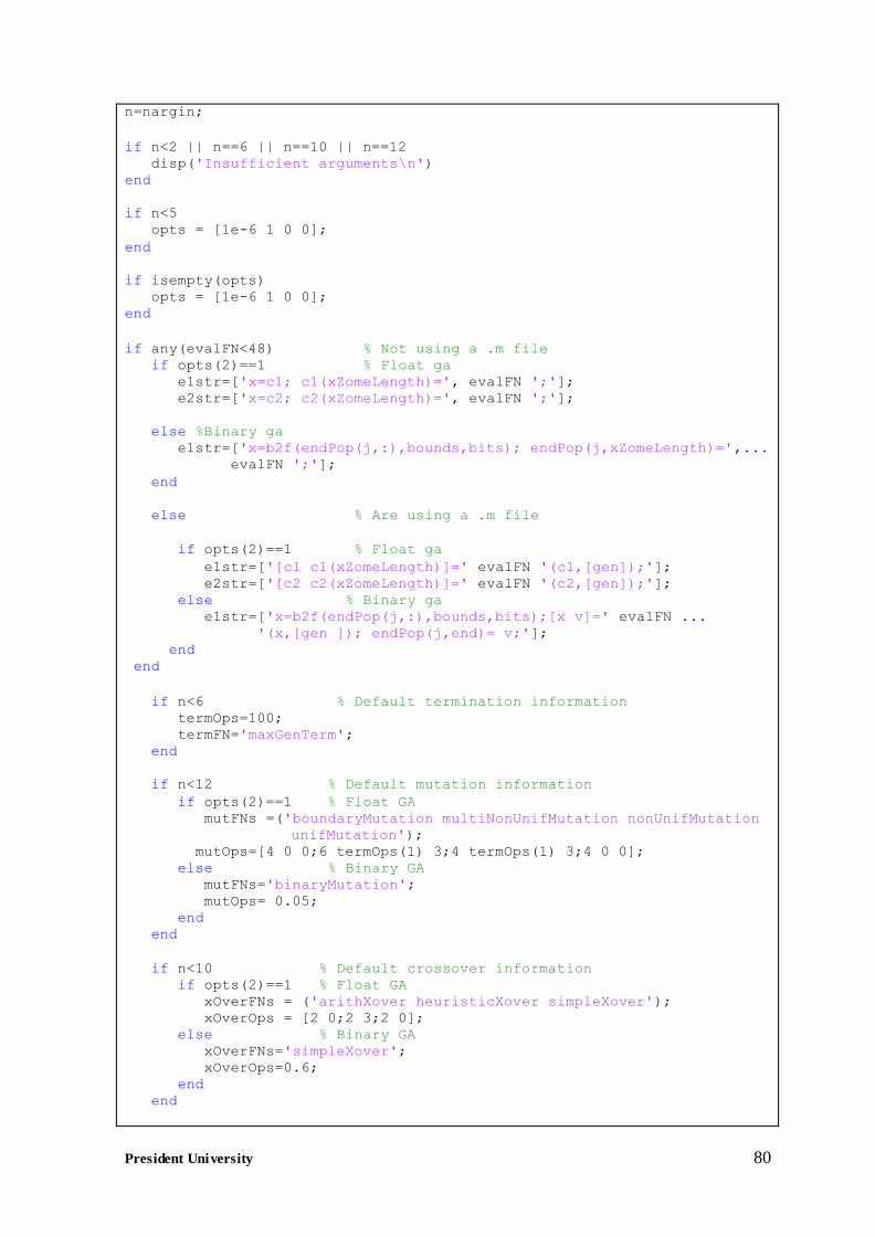
President University 80 President University
n=nargin;
if n<2 || n==6 || n==10 || n==12 disp('Insufficient arguments\n') end
if n<5
opts = [1e-6 1 0 0];
end
if isempty(opts) opts = [1e-6 1 0 0];
end
if any(evalFN<48) % Not using a .m file if opts(2)==1 % Float ga e1str=['x=c1; c1(xZomeLength)=', evalFN ';'];
e2str=['x=c2; c2(xZomeLength)=', evalFN ';'];
else %Binary ga e1str=['x=b2f(endPop(j,:),bounds,bits); endPop(j,xZomeLength)=',... evalFN ';'];
end
else % Are using a .m file
if opts(2)==1 % Float ga
e1str=['[c1 c1(xZomeLength)]=' evalFN '(c1,[gen]);']; e2str=['[c2 c2(xZomeLength)]=' evalFN '(c2,[gen]);'];
else % Binary ga e1str=['x=b2f(endPop(j,:),bounds,bits);[x v]=' evalFN ... '(x,[gen ]); endPop(j,end)= v;'];
end end
if n<6 % Default termination information
termOps=100; termFN='maxGenTerm'; end
if n<12 % Default mutation information
if opts(2)==1 % Float GA mutFNs =('boundaryMutation multiNonUnifMutation nonUnifMutation
unifMutation');
mutOps=[4 0 0;6 termOps(1) 3;4 termOps(1) 3;4 0 0]; else % Binary GA
mutFNs='binaryMutation'; mutOps= 0.05; end
end
if n<10 % Default crossover information if opts(2)==1 % Float GA xOverFNs = ('arithXover heuristicXover simpleXover');
xOverOps = [2 0;2 3;2 0]; else % Binary GA
xOverFNs='simpleXover'; xOverOps=0.6; end
end
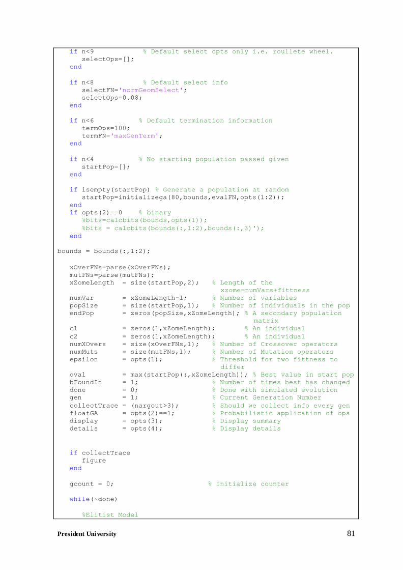
President University 81 President University
if n<9 % Default select opts only i.e. roullete wheel. selectOps=[];
end
if n<8 % Default select info
selectFN='normGeomSelect'; selectOps=0.08;
end
if n<6 % Default termination information
termOps=100; termFN='maxGenTerm';
end
if n<4 % No starting population passed given startPop=[]; end
if isempty(startPop) % Generate a population at random
startPop=initializega(80,bounds,evalFN,opts(1:2)); end if opts(2)==0 % binary
%bits=calcbits(bounds,opts(1));
%bits = calcbits(bounds(:,1:2),bounds(:,3)');
end
bounds = bounds(:,1:2);
xOverFNs=parse(xOverFNs);
mutFNs=parse(mutFNs); xZomeLength = size(startPop,2); % Length of the
xzome=numVars+fittness
numVar = xZomeLength-1; % Number of variables popSize = size(startPop,1); % Number of individuals in the pop
endPop = zeros(popSize,xZomeLength); % A secondary population
matrix c1 = zeros(1,xZomeLength); % An individual
c2 = zeros(1,xZomeLength); % An individual numXOvers = size(xOverFNs,1); % Number of Crossover operators
numMuts = size(mutFNs,1); % Number of Mutation operators epsilon = opts(1); % Threshold for two fittness to
differ
oval = max(startPop(:,xZomeLength)); % Best value in start pop bFoundIn = 1; % Number of times best has changed
done = 0; % Done with simulated evolution gen = 1; % Current Generation Number
collectTrace = (nargout>3); % Should we collect info every gen
floatGA = opts(2)==1; % Probabilistic application of ops display = opts(3); % Display summary
details = opts(4); % Display details
if collectTrace figure
end
gcount = 0; % Initialize counter
while(~done)
%Elitist Model
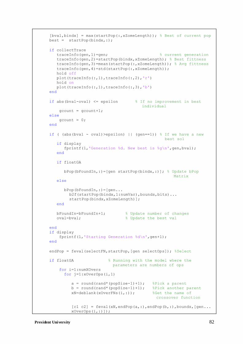
President University 82 President University
[bval,bindx] = max(startPop(:,xZomeLength)); % Best of current pop
best = startPop(bindx,:);
if collectTrace
traceInfo(gen,1)=gen; % current generation traceInfo(gen,2)=startPop(bindx,xZomeLength); % Best fittness
traceInfo(gen,3)=mean(startPop(:,xZomeLength)); % Avg fittness
traceInfo(gen,4)=std(startPop(:,xZomeLength));
hold off plot(traceInfo(:,1),traceInfo(:,2),'r') hold on
plot(traceInfo(:,1),traceInfo(:,3),'b') end
if abs(bval-oval) <= epsilon % If no improvement in best
individual
gcount = gcount+1; else
gcount = 0; end
if ( (abs(bval - oval)>epsilon) || (gen==1)) % If we have a new
best sol
if display
fprintf(1,'Generation %d. New best is %g\n',gen,bval); end
if floatGA
bPop(bFoundIn,:)=[gen startPop(bindx,:)]; % Update bPop
Matrix
else
bPop(bFoundIn,:)=[gen...
b2f(startPop(bindx,1:numVar),bounds,bits)...
startPop(bindx,xZomeLength)];
end
bFoundIn=bFoundIn+1; % Update number of changes
oval=bval; % Update the best val
end if display
fprintf(1,'Starting Generation %d\n',gen+1); end
endPop = feval(selectFN,startPop,[gen selectOps]); %Select
if floatGA % Running with the model where the
parameters are numbers of ops
for i=1:numXOvers for j=1:xOverOps(i,1)
a = round(rand*(popSize-1)+1); %Pick a parent b = round(rand*(popSize-1)+1); %Pick another parent
xN=deblank(xOverFNs(i,:)); %Get the name of
crossover function
[c1 c2] = feval(xN,endPop(a,:),endPop(b,:),bounds,[gen...
xOverOps(i,:)]);
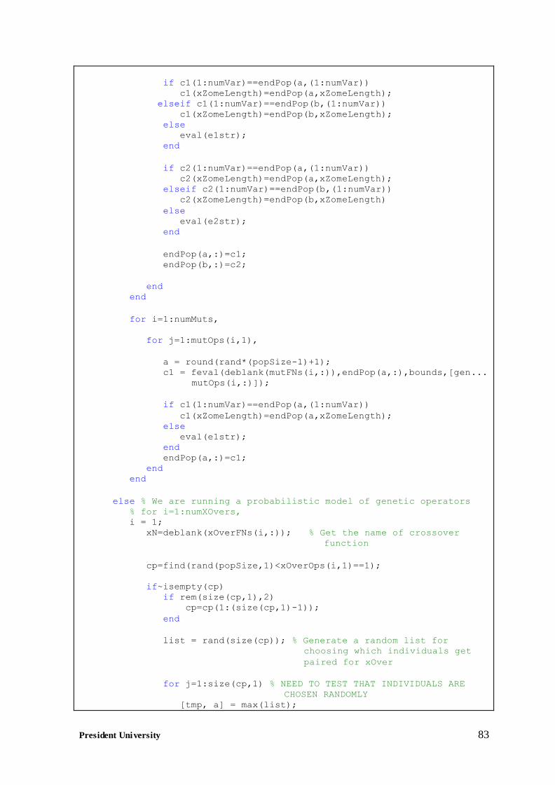
President University 83 President University
if c1(1:numVar)==endPop(a,(1:numVar))
c1(xZomeLength)=endPop(a,xZomeLength);
elseif c1(1:numVar)==endPop(b,(1:numVar))
c1(xZomeLength)=endPop(b,xZomeLength);
else eval(e1str);
end
if c2(1:numVar)==endPop(a,(1:numVar)) c2(xZomeLength)=endPop(a,xZomeLength); elseif c2(1:numVar)==endPop(b,(1:numVar))
c2(xZomeLength)=endPop(b,xZomeLength)
else
eval(e2str); end
endPop(a,:)=c1; endPop(b,:)=c2;
end end
for i=1:numMuts,
for j=1:mutOps(i,1),
a = round(rand*(popSize-1)+1); c1 = feval(deblank(mutFNs(i,:)),endPop(a,:),bounds,[gen...
mutOps(i,:)]);
if c1(1:numVar)==endPop(a,(1:numVar))
c1(xZomeLength)=endPop(a,xZomeLength); else
eval(e1str); end
endPop(a,:)=c1; end end
else % We are running a probabilistic model of genetic operators
% for i=1:numXOvers, i = 1; xN=deblank(xOverFNs(i,:)); % Get the name of crossover
function
cp=find(rand(popSize,1)<xOverOps(i,1)==1);
if~isempty(cp) if rem(size(cp,1),2) cp=cp(1:(size(cp,1)-1));
end
list = rand(size(cp)); % Generate a random list for
choosing which individuals get
paired for xOver
for j=1:size(cp,1) % NEED TO TEST THAT INDIVIDUALS ARE
CHOSEN RANDOMLY [tmp, a] = max(list);
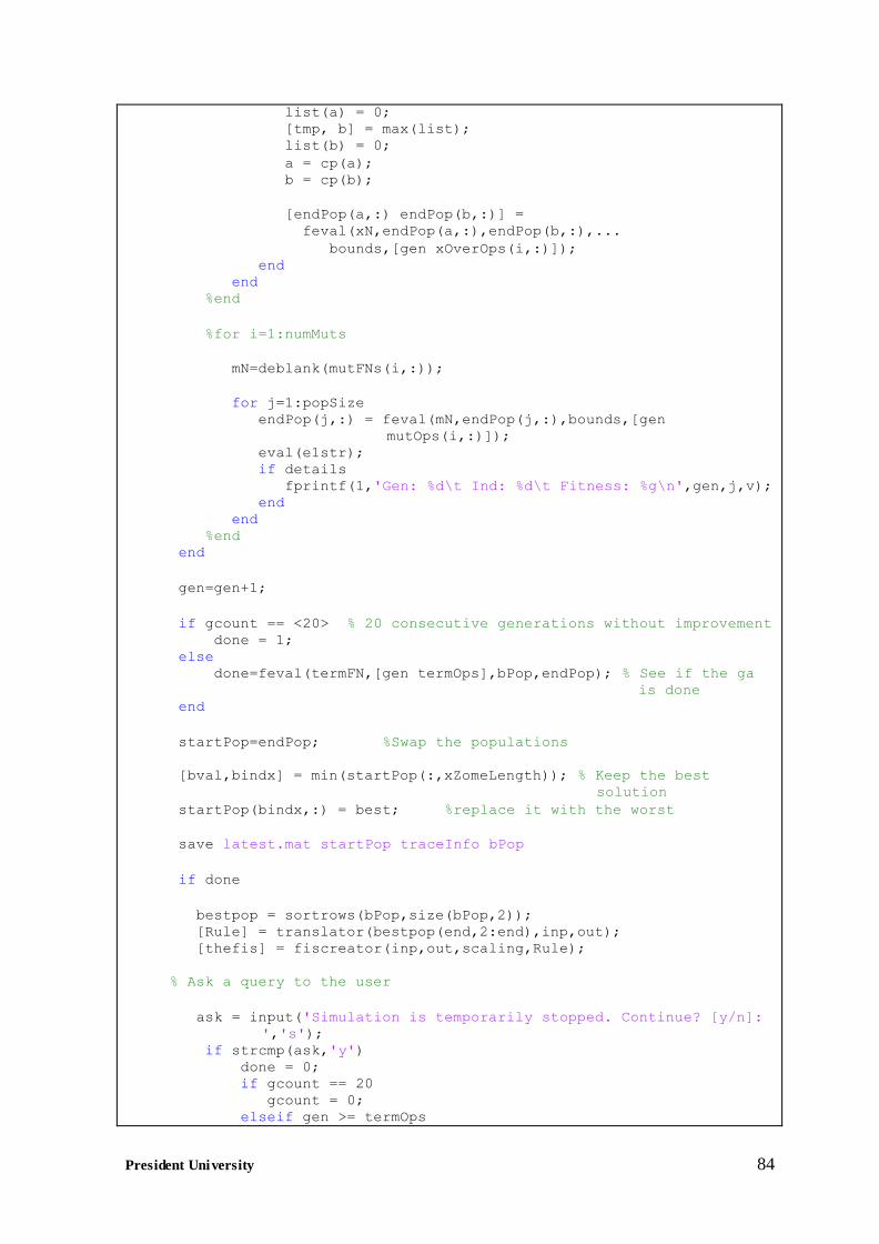
President University 84 President University
list(a) = 0; [tmp, b] = max(list);
list(b) = 0;
a = cp(a); b = cp(b);
[endPop(a,:) endPop(b,:)] =
feval(xN,endPop(a,:),endPop(b,:),...
bounds,[gen xOverOps(i,:)]);
end end %end
%for i=1:numMuts
mN=deblank(mutFNs(i,:));
for j=1:popSize endPop(j,:) = feval(mN,endPop(j,:),bounds,[gen
mutOps(i,:)]); eval(e1str); if details
fprintf(1,'Gen: %d\t Ind: %d\t Fitness: %g\n',gen,j,v); end
end %end end
gen=gen+1;
if gcount == <20> % 20 consecutive generations without improvement
done = 1; else done=feval(termFN,[gen termOps],bPop,endPop); % See if the ga
is done end
startPop=endPop; %Swap the populations
[bval,bindx] = min(startPop(:,xZomeLength)); % Keep the best
solution
startPop(bindx,:) = best; %replace it with the worst
save latest.mat startPop traceInfo bPop
if done
bestpop = sortrows(bPop,size(bPop,2));
[Rule] = translator(bestpop(end,2:end),inp,out); [thefis] = fiscreator(inp,out,scaling,Rule);
% Ask a query to the user
ask = input('Simulation is temporarily stopped. Continue? [y/n]:
','s'); if strcmp(ask,'y')
done = 0; if gcount == 20
gcount = 0; elseif gen >= termOps
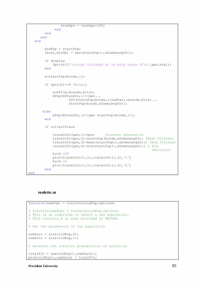
President University 85 President University
termOps = termOps+100; end
end
end end
endPop = startPop;
[bval,bindx] = max(startPop(:,xZomeLength));
if display fprintf('\ntrial finished at %d with score %f\n',gen,bval); end
x=startPop(bindx,:);
if opts(2)==0 %binary
x=b2f(x,bounds,bits); bPop(bFoundIn,:)=[gen...
b2f(startPop(bindx,1:numVar),bounds,bits)...
startPop(bindx,xZomeLength)];
else bPop(bFoundIn,:)=[gen startPop(bindx,:)];
end
if collectTrace
traceInfo(gen,1)=gen; %current generation
traceInfo(gen,2)=startPop(bindx,xZomeLength); %Best fittness traceInfo(gen,3)=mean(startPop(:,xZomeLength)); %Avg fittness
traceInfo(gen,4)=std(startPop(:,xZomeLength)); % Std.
Deviation hold off
plot(traceInfo(:,1),traceInfo(:,2),'r') hold on
plot(traceInfo(:,1),traceInfo(:,3),'b') end end
roulette.m
function[newPop] = roulette(oldPop,options)
% function[newPop] = roulette(oldPop,options)
% This is an algorithm to select a new population.
% This roulette.m is also provided by MATLAB.
% Get the parameters of the population
numVars = size(oldPop,2); numSols = size(oldPop,1);
% Generate the relative probabilites of selection
totalFit = sum(oldPop(:,numVars)); prob=oldPop(:,numVars) / totalFit;
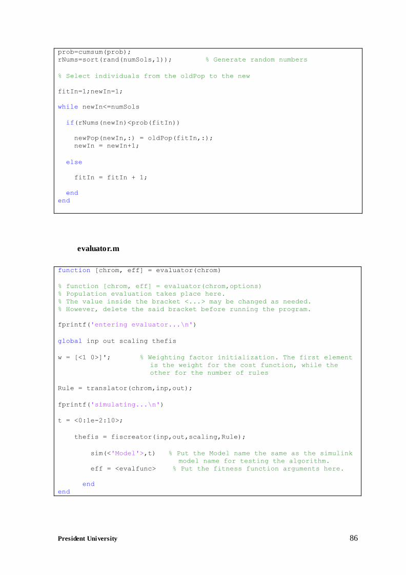
President University 86 President University
prob=cumsum(prob); rNums=sort(rand(numSols,1)); % Generate random numbers
% Select individuals from the oldPop to the new
fitIn=1;newIn=1;
while newIn<=numSols
if(rNums(newIn)<prob(fitIn))
newPop(newIn,:) = oldPop(fitIn,:);
newIn = newIn+1;
else
fitIn = fitIn + 1;
end
end
evaluator.m
function [chrom, eff] = evaluator(chrom)
% function [chrom, eff] = evaluator(chrom,options)
% Population evaluation takes place here.
% The value inside the bracket <...> may be changed as needed.
% However, delete the said bracket before running the program.
fprintf('entering evaluator...\n')
global inp out scaling thefis
w = [<1 0>]'; % Weighting factor initialization. The first element
is the weight for the cost function, while the
other for the number of rules
Rule = translator(chrom,inp,out);
fprintf('simulating...\n')
t = <0:1e-2:10>;
thefis = fiscreator(inp,out,scaling,Rule);
sim(<'Model'>,t) % Put the Model name the same as the simulink
model name for testing the algorithm.
eff = <evalfunc> % Put the fitness function arguments here.
end
end
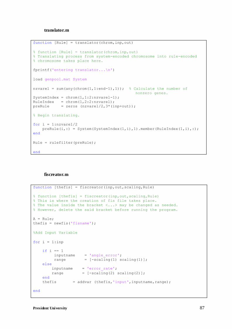
President University 87 President University
translator.m
function [Rule] = translator(chrom,inp,out)
% function [Rule] = translator(chrom,inp,out)
% Translating process from system-encoded chromosome into rule-encoded
% chromosome takes place here.
fprintf('entering translator...\n')
load genpool.mat System
nzvarel = sum(any(chrom(1,1:end-1),1)); % Calculate the number of
nonzero genes. SystemIndex = chrom(1,1:2:nzvarel-1); RuleIndex = chrom(1,2:2:nzvarel);
preRule = zeros (nzvarel/2,3*(inp+out));
% Begin translating.
for i = 1:nzvarel/2
preRule(i,:) = System(SystemIndex(1,i),1).member(RuleIndex(1,i),:); end
Rule = rulefilter(preRule);
end
fiscreator.m
function [thefis] = fiscreator(inp,out,scaling,Rule)
% function [thefis] = fiscreator(inp,out,scaling,Rule)
% This is where the creation of fis file takes place.
% The value inside the bracket <...> may be changed as needed.
% However, delete the said bracket before running the program.
A = Rule; thefis = newfis('fisname');
%Add Input Variable
for i = 1:inp
if i == 1 inputname = 'angle_error';
range = [-scaling(1) scaling(1)]; else
inputname = 'error_rate';
range = [-scaling(2) scaling(2)]; end
thefis = addvar (thefis,'input',inputname,range);
end
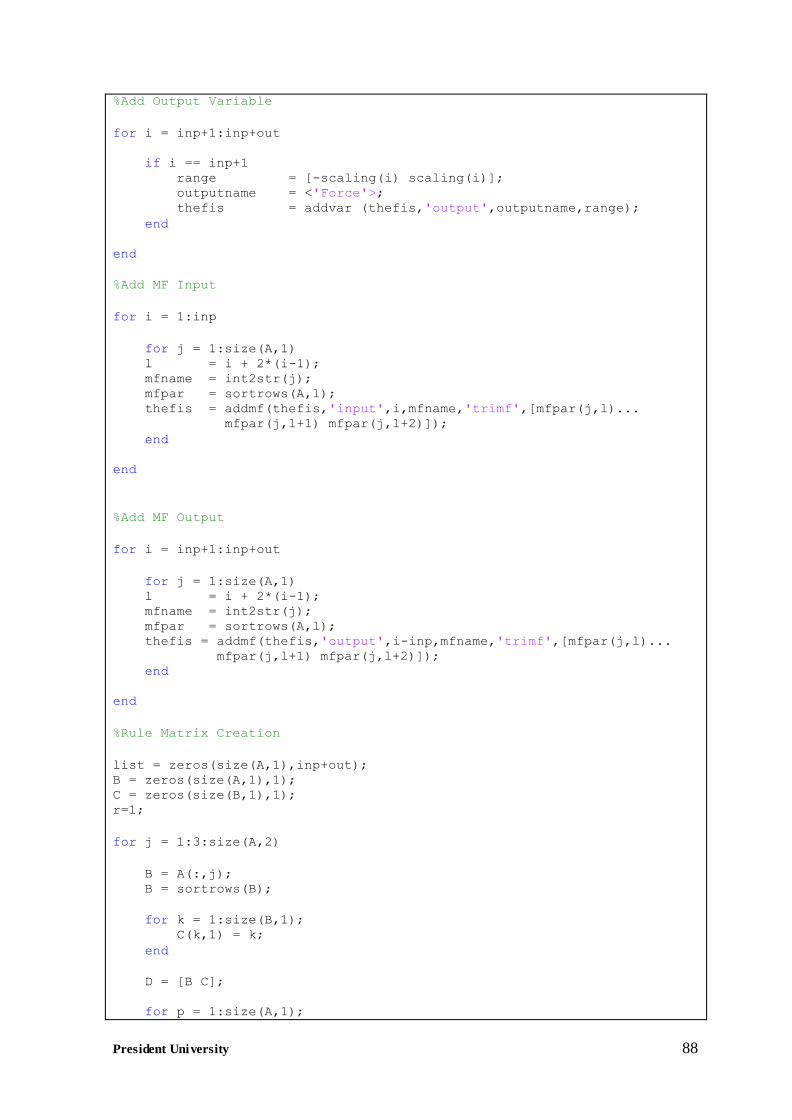
President University 88 President University
%Add Output Variable
for i = inp+1:inp+out
if i == inp+1
range = [-scaling(i) scaling(i)]; outputname = <'Force'>;
thefis = addvar (thefis,'output',outputname,range);
end
end
%Add MF Input
for i = 1:inp
for j = 1:size(A,1)
l = i + 2*(i-1); mfname = int2str(j);
mfpar = sortrows(A,l); thefis = addmf(thefis,'input',i,mfname,'trimf',[mfpar(j,l)...
mfpar(j,l+1) mfpar(j,l+2)]);
end
end
%Add MF Output
for i = inp+1:inp+out
for j = 1:size(A,1) l = i + 2*(i-1); mfname = int2str(j);
mfpar = sortrows(A,l); thefis = addmf(thefis,'output',i-inp,mfname,'trimf',[mfpar(j,l)...
mfpar(j,l+1) mfpar(j,l+2)]); end
end
%Rule Matrix Creation
list = zeros(size(A,1),inp+out); B = zeros(size(A,1),1); C = zeros(size(B,1),1);
r=1;
for j = 1:3:size(A,2)
B = A(:,j); B = sortrows(B);
for k = 1:size(B,1); C(k,1) = k;
end
D = [B C];
for p = 1:size(A,1);
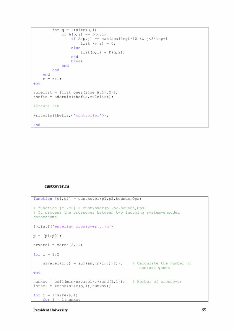
President University 89 President University
for q = 1:size(D,1) if A(p,j) == D(q,1)
if A(p,j) == max(scaling)*10 && j<3*inp+1
list (p,r) = 0; else
list(p,r) = D(q,2); end
break end end
end r = r+1;
end
rulelist = [list ones(size(A,1),2)]; thefis = addrule(thefis,rulelist);
%Create FIS
writefis(thefis,<'controller'>);
end
custxover.m
function [c1,c2] = custxover(p1,p2,bounds,Ops)
% function [c1,c2] = custxover(p1,p2,bounds,Ops)
% It process the crossover between two incoming system-encoded
chromosome.
fprintf('entering crossover...\n')
p = [p1;p2];
nzvarel = zeros(2,1);
for i = 1:2
nzvarel(i,:) = sum(any(p(i,:),1)); % Calculate the number of
nonzero genes
end
numxov = ceil(min(nzvarel).*rand(1,1)); % Number of crossover intsel = zeros(size(p,1),numxov);
for i = 1:size(p,1) for j = 1:numxov
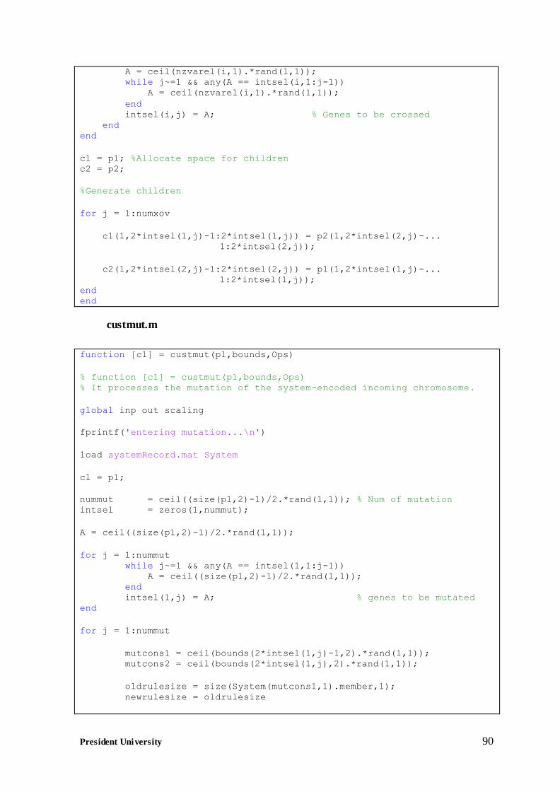
President University 90 President University
A = ceil(nzvarel(i,1).*rand(1,1)); while j~=1 && any(A == intsel(i,1:j-1))
A = ceil(nzvarel(i,1).*rand(1,1));
end intsel(i,j) = A; % Genes to be crossed
end end
c1 = p1; %Allocate space for children
c2 = p2;
%Generate children
for j = 1:numxov
c1(1,2*intsel(1,j)-1:2*intsel(1,j)) = p2(1,2*intsel(2,j)-...
1:2*intsel(2,j));
c2(1,2*intsel(2,j)-1:2*intsel(2,j)) = p1(1,2*intsel(1,j)-...
1:2*intsel(1,j)); end
end
custmut.m
function [c1] = custmut(p1,bounds,Ops)
% function [c1] = custmut(p1,bounds,Ops)
% It processes the mutation of the system-encoded incoming chromosome.
global inp out scaling
fprintf('entering mutation...\n')
load systemRecord.mat System
c1 = p1;
nummut = ceil((size(p1,2)-1)/2.*rand(1,1)); % Num of mutation intsel = zeros(1,nummut);
A = ceil((size(p1,2)-1)/2.*rand(1,1));
for j = 1:nummut
while j~=1 && any(A == intsel(1,1:j-1)) A = ceil((size(p1,2)-1)/2.*rand(1,1)); end
intsel(1,j) = A; % genes to be mutated end
for j = 1:nummut
mutcons1 = ceil(bounds(2*intsel(1,j)-1,2).*rand(1,1)); mutcons2 = ceil(bounds(2*intsel(1,j),2).*rand(1,1));
oldrulesize = size(System(mutcons1,1).member,1);
newrulesize = oldrulesize
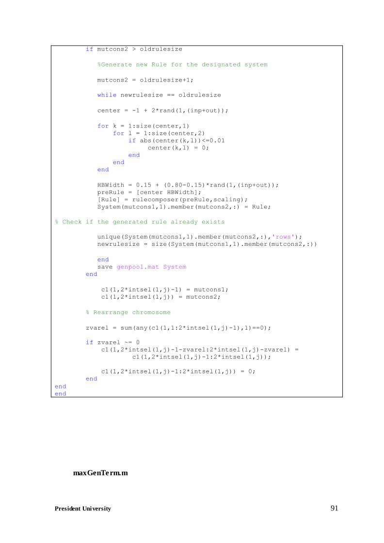
President University 91 President University
if mutcons2 > oldrulesize
%Generate new Rule for the designated system
mutcons2 = oldrulesize+1;
while newrulesize == oldrulesize
center = -1 + 2*rand(1,(inp+out));
for k = 1:size(center,1) for l = 1:size(center,2)
if abs(center(k,l))<=0.01 center(k,l) = 0;
end end end
HBWidth = 0.15 + (0.80-0.15)*rand(1,(inp+out));
preRule = [center HBWidth]; [Rule] = rulecomposer(preRule,scaling);
System(mutcons1,1).member(mutcons2,:) = Rule;
% Check if the generated rule already exists
unique(System(mutcons1,1).member(mutcons2,:),'rows');
newrulesize = size(System(mutcons1,1).member(mutcons2,:))
end
save genpool.mat System end
c1(1,2*intsel(1,j)-1) = mutcons1;
c1(1,2*intsel(1,j)) = mutcons2;
% Rearrange chromosome
zvarel = sum(any(c1(1,1:2*intsel(1,j)-1),1)==0);
if zvarel ~= 0 c1(1,2*intsel(1,j)-1-zvarel:2*intsel(1,j)-zvarel) =
c1(1,2*intsel(1,j)-1:2*intsel(1,j));
c1(1,2*intsel(1,j)-1:2*intsel(1,j)) = 0; end
end
end
maxGenTerm.m
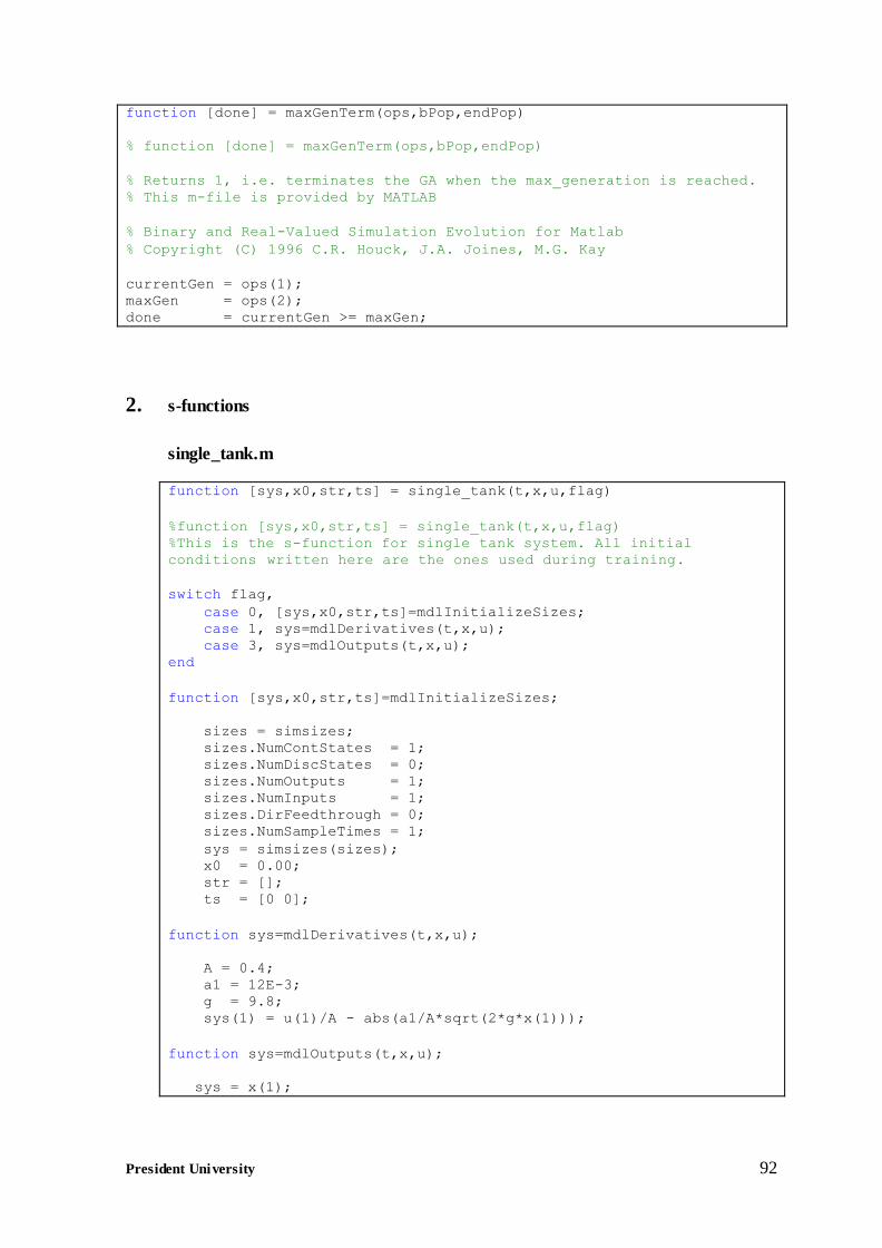
President University 92 President University
function [done] = maxGenTerm(ops,bPop,endPop)
% function [done] = maxGenTerm(ops,bPop,endPop)
% Returns 1, i.e. terminates the GA when the max_generation is reached.
% This m-file is provided by MATLAB
% Binary and Real-Valued Simulation Evolution for Matlab
% Copyright (C) 1996 C.R. Houck, J.A. Joines, M.G. Kay
currentGen = ops(1); maxGen = ops(2);
done = currentGen >= maxGen;
2. s-functions
single_tank.m
function [sys,x0,str,ts] = single_tank(t,x,u,flag)
%function [sys,x0,str,ts] = single_tank(t,x,u,flag) %This is the s-function for single tank system. All initial
conditions written here are the ones used during training.
switch flag,
case 0, [sys,x0,str,ts]=mdlInitializeSizes; case 1, sys=mdlDerivatives(t,x,u);
case 3, sys=mdlOutputs(t,x,u);
end
function [sys,x0,str,ts]=mdlInitializeSizes;
sizes = simsizes; sizes.NumContStates = 1;
sizes.NumDiscStates = 0; sizes.NumOutputs = 1; sizes.NumInputs = 1;
sizes.DirFeedthrough = 0; sizes.NumSampleTimes = 1;
sys = simsizes(sizes); x0 = 0.00;
str = [];
ts = [0 0];
function sys=mdlDerivatives(t,x,u);
A = 0.4;
a1 = 12E-3; g = 9.8;
sys(1) = u(1)/A - abs(a1/A*sqrt(2*g*x(1)));
function sys=mdlOutputs(t,x,u);
sys = x(1);
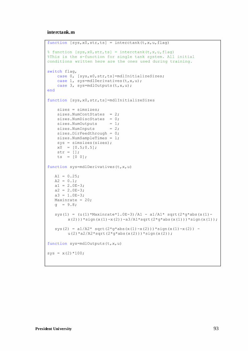
President University 93 President University
interctank.m
function [sys,x0,str,ts] = interctank(t,x,u,flag)
% function [sys,x0,str,ts] = interctank(t,x,u,flag)
%This is the s-function for single tank system. All initial
conditions written here are the ones used during training.
switch flag,
case 0, [sys,x0,str,ts]=mdlInitializeSizes;
case 1, sys=mdlDerivatives(t,x,u);
case 3, sys=mdlOutputs(t,x,u);
end
function [sys,x0,str,ts]=mdlInitializeSizes
sizes = simsizes;
sizes.NumContStates = 2; sizes.NumDiscStates = 0;
sizes.NumOutputs = 1;
sizes.NumInputs = 2;
sizes.DirFeedthrough = 0; sizes.NumSampleTimes = 1; sys = simsizes(sizes);
x0 = [0.5;0.5];
str = [];
ts = [0 0];
function sys=mdlDerivatives(t,x,u)
A1 = 0.25;
A2 = 0.1; a1 = 2.0E-3; a2 = 2.0E-3;
a3 = 1.0E-3; Maxinrate = 20;
g = 9.8;
sys(1) = (u(1)*Maxinrate*1.0E-3)/A1 - a1/A1* sqrt(2*g*abs(x(1)-
x(2)))*sign(x(1)-x(2))-a3/A1*sqrt(2*g*abs(x(1)))*sign(x(1));
sys(2) = a1/A2* sqrt(2*g*abs(x(1)-x(2)))*sign(x(1)-x(2)) -
u(2)*a2/A2*sqrt(2*g*abs(x(2)))*sign(x(2));
function sys=mdlOutputs(t,x,u)
sys = x(2)*100;
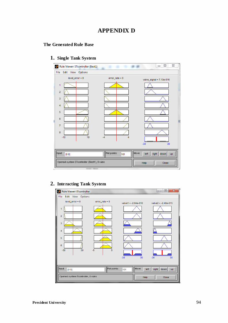
President University 94 President University
APPENDIX D
The Generated Rule Base
1. Single Tank System
2. Interacting Tank System
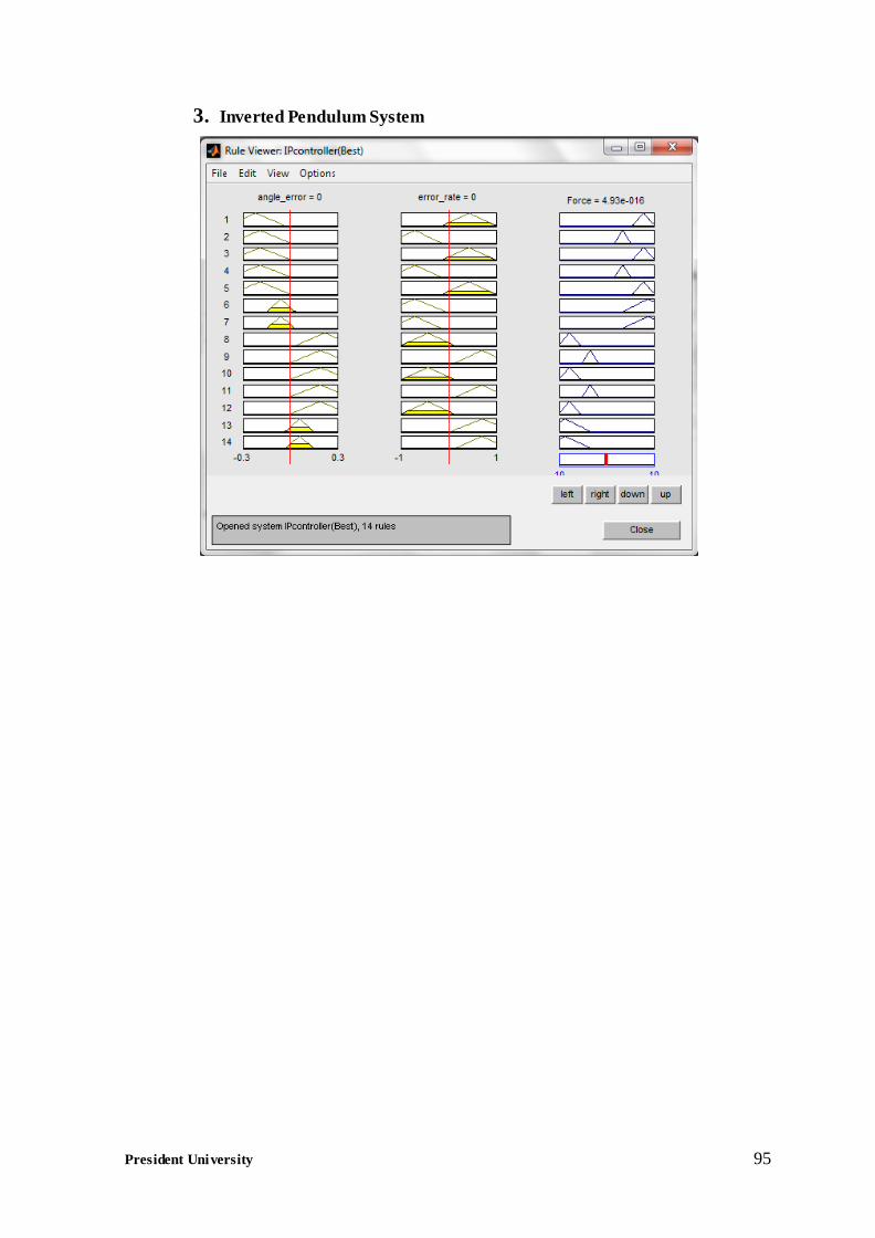
President University 95 President University
3. Inverted Pendulum System