
Final Report - The Crown Estate€¦ · An Investigation of EMF Generated by Subsea Windfarm Power...
71
CMACS/University of Liverpool & Econnect/J2733/Final_v1/07-2003 1 COWRIE-EMF-01-2002 A BASELINE ASSESSMENT OF ELECTROMAGNETIC FIELDS GENERATED BY OFFSHORE WINDFARM CABLES FINAL REPORT PREPARED BY: CENTRE FOR MARINE AND COASTAL STUDIES CENTRE FOR INTELLIGENT MONITORING SYSTEMS APPLIED ECOLOGY RESEARCH GROUP (All University of Liverpool) & ECONNECT LTD JULY 2003 J2733/V1/07-03 This report has been commissioned by COWRIE Centre for Marine and Coastal Studies University of Liverpool Vanguard Way Birkenhead CH41 9HX Tel: 0151 650 2275 Fax: 0151 650 2274 E-mail: [email protected]
Transcript of Final Report - The Crown Estate€¦ · An Investigation of EMF Generated by Subsea Windfarm Power...

An Investigation of EMF Generated by Subsea Windfarm Power Cables
CMACS/University of Liverpool & Econnect/J2733/Final_v1/07-2003 1
COWRIE-EMF-01-2002
A BASELINE ASSESSMENT OF ELECTROMAGNETIC FIELDS GENERATED BY OFFSHORE WINDFARM CABLES
FINAL REPORT
PREPARED BY:
CENTRE FOR MARINE AND COASTAL STUDIES
CENTRE FOR INTELLIGENT MONITORING SYSTEMS
APPLIED ECOLOGY RESEARCH GROUP
(All University of Liverpool)
&
ECONNECT LTD
JULY 2003 J2733/V1/07-03
This report has been commissioned by COWRIE
Centre for Marine and Coastal Studies University of Liverpool Vanguard Way Birkenhead CH41 9HX Tel: 0151 650 2275 Fax: 0151 650 2274 E-mail: [email protected]

An Investigation of EMF Generated by Subsea Windfarm Power Cables
CMACS/University of Liverpool & Econnect/J2733/Final_v1/07-2003 2
This report has been prepared by CMACS for COWRIE as part of the generic research programme
identified to benefit the offshore windfarm industry. The views and recommendations presented in this
report are not necessarily those of COWRIE, its individual members, or the organisations they
represent, who accordingly have no legal liability for its contents. Any reproduction in full or in part of this report must fully acknowledge COWRIE using the following
reference:
CMACS (2003) A baseline assessment of electromagnetic fields generated by offshore windfarm cables. COWRIE Report EMF - 01-2002 66.

An Investigation of EMF Generated by Subsea Windfarm Power Cables
CMACS/University of Liverpool & Econnect/J2733/Final_v1/07-2003 3
EXECUTIVE SUMMARY
COWRIE identified as priority research the issue of electromagnetic fields (EMF) generated by
offshore windfarm power cables and their possible effect on organisms that are sensitive to these
fields. A consortium, lead by CMACS, was contracted to carry out a Stage 1 investigation to
investigate the following:
• The likely EMF emitted from a subsea power cable.
• A suggested method to measure EMF in the field, which could be applied by windfarm developers
or in future projects.
• Guidance on mitigation measures to reduce EMF.
• Consideration of the results for the next stage of investigation into the effects of EMF on electro-
sensitive species.
An assessment of existing publications (both hard and electronic) and direct communications
regarding EMF emitted by undersea power cables suggested that the current state of knowledge is too
variable and inconclusive to make an informed assessment of any possible environmental impact of
EMF in the range of values likely to be detected by organisms sensitive to electric and magnetic fields.
Therefore modelling and direct measurement of the electric and magnetic field components of EMF
was undertaken.
An Alternating Current (AC) Conduction Field Solver model and Eddy Current Field Solver model
were used within the 'Maxwell 2D' software program which allows the simulation of electromagnetic
and electrostatic fields in structures with uniform cross-sections by solving Maxwell’s equations using
the finite-element method. The modelling was based on EMF generated by a 132kV XLPE three-
phase submarine cable designed by Pirelli with an AC current of 350 amps buried at a depth of 1m.
The results of the model simulations showed that a cable with perfect shielding i.e. where conductor
sheathes are grounded, does not generate an electric field (E-field) directly. However, a magnetic field
(B-field) is generated in the local environment by the alternating current in the cable. This in turn,
generates an induced E-field close to the cable within the range detectable by electro-sensitive fish
species. Simulations with non-perfect shielding, i.e. where there is poor grounding of sheathes,
showed that there is a leakage E-field, but it is smaller than the induced E-fields and unlikely to be
additive.

An Investigation of EMF Generated by Subsea Windfarm Power Cables
CMACS/University of Liverpool & Econnect/J2733/Final_v1/07-2003 4
A method is provided for calculating the induced E-field around a low frequency AC power cable due
to the emanating B-field. This method requires in situ measurement of the B-field generated by an
operational cable.
To consider mitigation, the models simulated changes in permeability of the power cable armour and
conductivity of the cable sheath and armour. The model predicted that as the permeability of the
armour increased the resultant EMF strength outside the cable decreased. The model also showed that
a non-linear relationship exists between electromagnetic field strength adjacent to the cable and
permeability of the armouring material. This indicated that using materials with very high permeability
values for armouring of submarine power cables could help to reduce the EMF generated to below the
lowest known level that electroreceptive elasmobranchs can detect. As the conductivity of the armour
was increased the model showed that the resultant EMF strength outside the cable decreased. A linear
relationship was found between electromagnetic field strength and the conductivity of the materials
used in the cable. These results indicate that a reduction in the strength of the electromagnetic fields
induced by a three-phase 132kV XLPE submarine cable can be achieved through the application of
materials with high conductivity and high permeability. These results provide useful information for
consideration during the design and manufacture of submarine cables with reduced EMF emissions.
Burial was shown to be ineffective in ‘dampening’ the B-field, however cable burial to a depth of at
least 1m is likely to provide some mitigation for the possible impacts of the strongest B-field and
induced E-fields (that exist within millimetres of the cable) on sensitive fish species, owing to the
physical barrier of the substratum.
An additional mitigation consideration is the use of substations to convert the voltage from 33kV to
132kV would reduce the current carried by a cable and would therefore reduce the induced E-fields by
a factor of four. This could be used to add to mitigation of the EMF effects of sending power to the
shore but probably has practical and economic limitations.
In terms of the potential significance of the modelled results to electrosensitive fish the following
conclusions were made:
• EMF emitted by an industry standard three-core power cable will induce E-fields.
• In the case modelled, this resulted in a predicted E-field of approximately 91μV/m (=0.9 μV/cm)
in seawater above a cable buried to 1m. This level of E-field is on the boundary of E-field
emissions that are expected to attract and those that repel elasmobranchs (the most widespread
electrosensitive fish group of UK coastal waters).
• In addition, the induced E-fields calculated from the B-fields measured in situ were also within
the lower range of detection by elasmobranchs.

An Investigation of EMF Generated by Subsea Windfarm Power Cables
CMACS/University of Liverpool & Econnect/J2733/Final_v1/07-2003 5
• The options for mitigation using either changes in permeability or conductivity indicate that the
induced E-field can be effectively reduced. However, unless highly specialised materials and
manufacturing process are used with high permeability values, the E-field will still remain within
the lower range of detection of elasmobranchs. Hence any reduction in E-field emission using
existing materials could minimise the potential for an avoidance reaction by a fish if it
encountered the field but may still result in an attraction response.
• Another important consideration is the relationship between the amount of cable, either buried or
unburied, producing induced E-fields and the available habitat of an electrosensitive species.
• There is also a need to determine if the power cable operating frequency (50Hz) and associated
sub-harmonic frequencies have any effect on the EMFs that are detectable by UK electrosensitive
fishes.
Finally, a number of further studies are recommended to direct future research to fully understand the
interaction of the induced E-fields from subsea power cables with electrosensitive fish and any
implications of the B-fields for organisms that rely on a magnetic sense.

An Investigation of EMF Generated by Subsea Windfarm Power Cables
CMACS/University of Liverpool & Econnect/J2733/Final_v1/07-2003 6
CONTENTS This report has been commissioned by COWRIE.................................................................... 1
1. INTRODUCTION........................................................................................................................ 10 1.1 Project Background ................................................................................................................ 10
2. REVIEW OF EXISTING INFORMATION ................................................................................. 12 2.1 UK Offshore Windfarm Cabling Strategies ............................................................................. 12
2.1.1 Factors affecting cabling strategies................................................................................... 12 2.1.2 Inter-turbine cables .......................................................................................................... 13 2.1.3 Array-to-shore cables....................................................................................................... 13
2.2 CURRENT UNDERSTANDING OF THE EMF generated by subsea power cables ............... 15 3. MODELLING EMF..................................................................................................................... 18
3.1 Introduction to the simulation software ................................................................................... 18 3.1.1 AC conduction field solver model .................................................................................... 19 3.1.2 Eddy current field solver model ....................................................................................... 20
3.2 Modelling of the cable ............................................................................................................ 21 3.2.1 Geometrical modelling of the problem ............................................................................. 21 3.2.2 Electromagnetic properties of the materials ...................................................................... 22
3.3 Simulation results and discussion............................................................................................ 24 3.3.1 EMF generated by a cable with perfect shielding.............................................................. 24
3.3.1.1 AC Conduction field solver model ............................................................................ 24 3.3.1.2 Eddy current field solver model................................................................................. 26
3.3.2 EMF generated by cables with non-perfect shielding........................................................ 31 3.4 Conclusions from modelling EMF with and without perfect cable shielding............................ 33
4. MEASURING EMF IN THE ENVIRONMENT........................................................................... 34 4.1 Introduction............................................................................................................................ 34 4.2 Designing the magnetic and electric field sensors.................................................................... 34
4.2.1 The Magnetic field sensor ................................................................................................ 34 4.2.2 The Electric field sensor................................................................................................... 34
4.2.2.1. The High input impedance electric field sensor......................................................... 35 4.2.2.2. The Low input impedance electric field sensor ......................................................... 35
4.3 Laboratory testing................................................................................................................... 37 4.4 Field testing............................................................................................................................ 40
4.4.1 Introduction ..................................................................................................................... 40 4.4.2 Methodology ................................................................................................................... 40
4.5 Results ................................................................................................................................... 42 4.5.1 Magnetic field sensor ....................................................................................................... 42

An Investigation of EMF Generated by Subsea Windfarm Power Cables
CMACS/University of Liverpool & Econnect/J2733/Final_v1/07-2003 7
4.5.2 Electric field sensor ......................................................................................................... 43 4.6 Methodology for calculation of EMF...................................................................................... 44 4.7 Conclusions drawn from measuring EMF ............................................................................... 45
5. MITIGATION FOR EMF ............................................................................................................ 47 5.1 Effects of permeability of the cable armour............................................................................. 47 5.2. Effects of conductivity of the cable sheath and armour........................................................... 50 5.3 Effects of cable burial............................................................................................................. 53 5.4 Conclusions CONCERNING MITIGATION.......................................................................... 55
6. CONSIDERATION OF THE RESULTS WITH RESPECT TO FISH SENSITIVE TO
ELECTROMAGNETIC FIELDS..................................................................................................... 56 6.1. Response to electric fields...................................................................................................... 56 6.2. Response to magnetic fields................................................................................................... 58
7. RECOMMENDATIONS FOR FURTHER STUDIES .................................................................. 59 7.1. Electrical Engineering studies ................................................................................................ 59 7.2. Biological studies .................................................................................................................. 59
8. OVERALL CONCLUSIONS....................................................................................................... 61 Species....................................................................................................................................... 70
10. APPENDICES……………………………………………………………………………………..66

An Investigation of EMF Generated by Subsea Windfarm Power Cables
CMACS/University of Liverpool & Econnect/J2733/Final_v1/07-2003 8
GLOSSARY OF TERMS
RMS The ‘square root of the mean squared’ used by engineers to describe levels of alternating signals. ie.
Current flow in power cables goes first in one direction then reverses. RMS is the equivalent current flowing in one direction continuously that would supply the same amount of electrical power.
Note: The peak of the alternating signal is typically 1.4 times larger than its RMS value
Voltage
Voltage (V) is a measurement of the electrical potential difference that exists between two points. 1,000,000 μV = 1,000 mV = 1 V
μV micro-volts mV milli-volts
Electric field (E) Electric field (V/m) is a measure of how the voltage changes when a measurement point is moved in
a given direction. If no direction is stated then the direction can be assumed to be the one that produces the largest change. 1 μV/cm = 100 μV/m 1,000,000 μV/m = 1000 mV/m = 1 V/m
Current (A) An electric charge in motion (amps) AC Alternating current (or voltage) i.e. flows forward then backwards at 50 times per second (Hz) DC Direct current i.e. flows in the same direction all the time. ( 0 Hz) Current density Current density (A/m²) is analogous to water flow. It is a measure of how much electrical current in
amps (A) is flowing through a given area.
Magnetic field (H) Magnetic field (A/m) is analogous to water flow. It is directly linked to the magnetic flux density (B) that is flowing in a given direction. If no direction is stated then it can be assumed to be the direction that produces the largest the magnetic field. B = µ H, where µ is the permeability of the material. The SI unit for magnetic flux density B is tesla (T) 1 T = 1 Wb/m² 1,000,000,000 nT = 1,000,000 μT = 1,000 mT = 1 T
nT Nano-tesla μT Micro-tesla mT Milli-tesla
The Relationship between of various units at 50 Hz (in air or seawater ) nT (B) μT (B) Gauss (B) A/m (H) Applied Induced
E field (μV/m)
1 0.001 0.00001 0.000796 0.31 100 0.1 0.001 0.07958 31
125.7 0.1257 0.001257 0.1 39 1000 1 0.01 0.795798 314 1257 1.257 0.01257 1 395
10,000 10 0.1 8.0 3,142 100,000 100 1 79.6 31,416
3,000,000 3000 30 2,387.4 942,478

An Investigation of EMF Generated by Subsea Windfarm Power Cables
CMACS/University of Liverpool & Econnect/J2733/Final_v1/07-2003 9
REPORT STRUCTURE • Section 1 sets the context of the project.
• Section 2 describes cabling strategies for UK offshore windfarms, existing information on EMF
generated by subsea power cables and projects that have been carried out in Europe to date.
• Section 3 describes the modelling of EMF generated by subsea power cables for a typical UK
offshore windfarm power-cabling scenario.
• Section 4 describes the development and construction of electric and magnetic field sensors
constructed for a preliminary investigation into in-situ EMF generated by subsea power cables and
gives a method by which EMF can be calculated by windfarm developers.
• Section 5 considers possible areas of mitigation for the reduction of EMF.
• Section 6 discusses the results of the studies in the context of electro-sensitive fish species.
• Section 7 makes recommendations for future studies.
• Section 8 gives overall conclusions of the investigation.
• Section 9 provides the cited references in numerical order of use in the text.
• Section 10 has the appendices with details of the people and organisations contacted; electrical
circuits for the sensors; and a list of electrosensitive fish species of UK coastal waters.
An Investigation of EMF Generated by Subsea Windfarm Power Cables
CMACS/University of Liverpool & Econnect/J2733/Final_v1/07-2003 10
1. INTRODUCTION
In April 2001, eighteen companies successfully pre-qualified for an option to lease areas of the seabed
in UK territorial waters from the Crown Estate for the development of offshore windfarms, the first of
their kind in the UK coastal zone.
The financial pre-qualification requirements for these eighteen sites initiated the establishment of a
trust fund for the purposes of short to medium term, generic environmental studies to benefit the early
stages of the offshore windfarm industry as a whole and provide guidance for future developments.
The fund is administered by the COWRIE (Collaborative Offshore Wind Research into the
Environment) steering group, which represents the offshore windfarm industry, NGO’s, GO's, DTI
and statutory conservation agencies.
COWRIE has identified a number of priority areas for generic research. One of these areas is the issue
of electromagnetic fields (EMF) generated by offshore windfarm power cables and their possible
effect on organisms that are sensitive to these fields.
A consortium of departments of the University of Liverpool and Econnect Ltd., lead by the Centre for
Marine and Coastal Studies (CMACS) was contracted by COWRIE to attempt to specifically identify
and quantify electromagnetic fields (EMF) generated by offshore windfarm subsea power cables. This
research was required as the first stage of studies that aim to provide a more informed and objective
assessment of the potential effects of EMF on organisms sensitive to both electric and magnetic fields.
1.1 PROJECT BACKGROUND
A preliminary investigation of the potential impacts of offshore windfarm power cables on electro-
sensitive fish was carried out at the University of Liverpool during 2001 for the Countryside Council
of Wales1. In this investigation, Gill & Taylor1 investigated the potential effect of EMF predicted to be
generated by subsea power cabling upon elasmobranch fishes (sharks, skates and rays). Owing to a
paucity of information in the literature they undertook a basic laboratory-based experiment to
investigate the response of the dogfish, Scyliorhinus canicula, to electric fields (E-fields) generated by
a direct current (DC) electrode placed in a seawater tank. Although their investigation was only a pilot
study the results were notable in that the dogfish avoided constant E-fields at 1000 micro-volts per
metre (µV/m), which were simulating the size of the EMF emission predicted from 150kVcables with
a current of 600A. The avoidance response by the dogfish was, however, variable amongst individuals
and had a relatively low probability of occurring in the conditions presented in Gill & Taylor's

An Investigation of EMF Generated by Subsea Windfarm Power Cables
CMACS/University of Liverpool & Econnect/J2733/Final_v1/07-2003 11
experiment. Importantly individuals of the same species were attracted to an E-field of 10µV/m at
0.1m from the source which is similar to the bioelectric fields emitted by dogfish prey.
Gill & Taylor made a number of recommendations based on the findings of their preliminary research.
These recommendations included the following:
• Electric field research, in particular the quantification of fields within different substrata and
in situ measurement.
• Further directed biological research, especially focussing on species that use inshore habitats
and behavioural responses to E-fields.
• GIS mapping and interrogation, to provide a database that can guide decisions on the location
of offshore windpower sites taking into account, amongst other factors the potential conflicts
with elasmobranchs and their resource requirements.
The COWRIE steering group recommended a two-stage approach to further research into EMF and its
possible ecological impact. Stage 1 required calculation of the EMF generated by power cables at the
seabed, an assessment of the effects of burial and/or shielding and some preliminary in-situ
measurements of EMF generated by an existing subsea power cable. The consortium, lead by
CMACS, was contracted to carry out the Stage 1 investigation to meet the following deliverables
under this contract:
• The likely EMF emitted from a subsea power cable.
• A suggested method to measure EMF in the field that could be applied by windfarm developers or
in future projects.
• Guidance on mitigation measures to reduce EMF.
• Consideration of the results for the next stage of investigation into the effects of EMF on electro-
sensitive species.
Due to time limitations, it was agreed with COWRIE at the start-up meeting that CMACS would
prioritise the modelling of EMF to a 132 kilo-volt (kV) Pirelli cable with an AC current of 350 amps
in the marine environment and cable burial at a depth of 1m, as this was the most common cabling
scenario. COWRIE also asked for consideration of EMF in brackish water environments, should
further windfarm proposals consider routing power cables in estuaries.

An Investigation of EMF Generated by Subsea Windfarm Power Cables
CMACS/University of Liverpool & Econnect/J2733/Final_v1/07-2003 12
2. REVIEW OF EXISTING INFORMATION
There is very little information available in the published literature or industry reports concerning
either measured EMF generated by subsea power cables or actual investigation of the impact of EMF
on species sensitive to these fields. This section of the report considers the available information that
was gathered from published papers, reports and through consultation with a number of organisations
and individuals (see Appendix I) and is broken down into two parts. Section 2.1 discusses UK offshore
windfarm cabling strategies in the context of the first phase of developments in the UK. Section 2.2
describes the existing information regarding EMF generated by subsea cables and the work that has
been carried out and/or planned for the future, in Europe.
2.1 UK OFFSHORE WINDFARM CABLING STRATEGIES
2.1.1 Factors affecting cabling strategies
The design of sub-sea cable systems for electricity produced by offshore windfarms will be influenced
by several factors. Some of the factors are generic, while others are project-specific:
• Utility connection voltage – The vast majority of the current windfarm projects will be connected
to regional distribution networks, rather than to the national transmission system. In England and
Wales, these distribution networks currently cover 132kV and 33kV systems, as well as local
11kV distribution networks. Some of the phase 1 projects have secured connections at 33kV;
others have secured connections at 132kV.
• Sub-sea cable technology – Three-core sub-sea cables using solid insulation (EPR or XLPE) are
available for operation at voltages up to 132kV. Higher voltage cables that use oil as an insulating
medium are not deemed to be environmentally acceptable owing to the potential risks associated
with oil leakage. Cables with conductor sizes from 50mm2 up to 630mm2 are generally available,
giving current carrying capacities up to approximately 700A. This equates to a power
transmission capacity of up to 40MW for a single 33kV cable, or 160MW for a 132kV cable.
• Turbine electrical design – Most of the developers of the phase 1 windfarm projects are planning
to use turbines rated at 2.75MW or more. These turbines are normally supplied with step-up
transformers, with various options of HV voltage. These options typically include 20kV, 33kV
and 36kV. Some HV switchgear is needed at the turbine, to protect the step-up transformer. This
limits the HV voltage at the turbines to 36kV, as switchgear for higher voltage levels is either
very large or very costly.
• Distance from shore – For large windfarm projects, the use of a single 132kV cable to shore can
be a cost-effective alternative to the use of three or four 33kV cables. The installed cost (per
kilometre) of a single 132kV cable is considerably lower than the installed cost of three 33kV

An Investigation of EMF Generated by Subsea Windfarm Power Cables
CMACS/University of Liverpool & Econnect/J2733/Final_v1/07-2003 13
cables, but this solution requires an offshore substation in order to step up to 132kV from the
windfarm collection voltage (usually 33kV). If the cable route to shore is short, the cost of the
substation outweighs the saving on the cable. However, the offshore substation can often be
justified if the cable route is much more than 10km. In addition, substations reduce the number of
cables required and therefore the area affected.
2.1.2 Inter-turbine cables
The function of the inter-turbine cables is to collect the power from all of the turbines and bring it to
one or more ‘collection points’ within the windfarm, from where it can be transmitted to shore. It is
normal practice to cable several turbines together in a ‘daisy chain’, with each cable providing a link
between two adjacent turbines. Each end of the cable is terminated onto the HV switchgear located
within the turbine tower. A number of features associated with these cables are:
• Cable voltage – Because they connect to the HV switchgear at the turbines, the operating voltage
for the inter-turbine cables is limited to 36kV. A nominal system voltage of 33kV is often
planned for use in the UK, as this facilitates connection to the 33kV distribution system on-shore.
• Cable sizing – The sizing of the inter-turbine cables depends on the design approach used for the
cable system. Some ‘tree-like’ designs involve the use of different cable sizes, with heavy cable
being used for the main branches in the tree, and lighter cable being used for minor branches
carrying the output from just one or two turbines. In ‘looped’ designs, the same cable size is often
used for all of the inter-turbine cables.
• Cable armour – Single-wire armouring (SWA) is normally specified for inter-turbine cables. This
level of armouring provides adequate protection against the kind of activities that are likely to
occur within the wind turbine array (e.g. small boat anchors, marker buoy moorings etc). Double
wire armoured (DWA) can be used but is heavy and inflexible cable such making it more difficult
and expensive to produce and lay. The specific armouring required will however depend on the
substratum type.
• Cable burial – Surface laying of the inter-turbine cables is normally deemed to be acceptable.
Burial of the cables is sometimes specified if there are specific risks to exposed cables. Examples
of such risks include sun damage to cables on sandbanks that are exposed at low tide, or cables
becoming ‘suspended’ across deep troughs or ripples in the seabed. The type of substratum that
the cable crosses will also determine whether cable burial is feasible (eg. sand versus rock).
2.1.3 Array-to-shore cables
The function of the array-to-shore cables is to transmit the power from the collection point (or points)
within the windfarm to an appropriate cable connection facility at the shoreline. The electrical
parameters of these cables will depend on the choice made between two options:

An Investigation of EMF Generated by Subsea Windfarm Power Cables
CMACS/University of Liverpool & Econnect/J2733/Final_v1/07-2003 14
Option A: No voltage step-up offshore – The power produced by the windfarm is transmitted to shore
at the collection system voltage. There is no need for an offshore substation. A few ‘root turbines’ act
as the collection points within the windfarm. Each array-to-shore cable runs from a ‘root turbine’ to
shore.
Option B: With voltage step-up offshore – The power produced by the windfarm is transmitted to
shore at a different voltage level, greater than the collection voltage. An offshore substation is
required, containing one or more step-up transformers. The offshore substation acts as the collection
point within the windfarm. Each array-to-shore cable runs from the offshore substation to shore.
A third option, high voltage direct current (HVDC) is not economically viable at present due to the
high cost of HVDC converters, however it may be used for sites situated further offshore in the future.
The design parameters of the array-to-shore cables can be discussed with reference to options A and
B.
• Cable voltage – Given option A, the operating voltage for the array-to-shore cables is limited to
36kV because of the HV switchgear in the turbines. Under option B, the limiting factor is the
availability of environmentally acceptable cable technology. At present, the limit is 132kV as
cables rated to operate above 132kV require the use of oil insulation.
• Cable sizing – Given option A, the array-to-shore cables will normally be sized to minimise the
number of cables required. This results in the use of very heavy cable (630mm2 or greater). For
option B, the size of the windfarm may not require the use of the heaviest cable. For example, a
100MW windfarm could be connected to shore using a single 300mm2 cable rated at 132kV.
• Cable armour – Either single- (SWA) or double-wire armouring (DWA) may be specified for
array-to-shore cables. Notwithstanding the costs and practical constraints of DWA, they tend to
be used if the cable route crosses hard ground (ie. rock) and there is a risk of crush damage.
Single-wire is often deemed to be adequate if the sea-bed is soft (sand or silt) and the cable is to
be buried.
• Cable burial – Burial of array-to-shore cables is usually regarded as prudent, due to the risk posed
by large vessels operating outside the windfarm boundary. Target depths of up to one metre are
usually as depths greater than this are difficult to achieve in anything harder than sand or silt.
Cable burial is costly, and this has to be weighed against the risks to the cable and the
consequences of major damage.

An Investigation of EMF Generated by Subsea Windfarm Power Cables
CMACS/University of Liverpool & Econnect/J2733/Final_v1/07-2003 15
2.2 CURRENT UNDERSTANDING OF THE EMF GENERATED BY SUBSEA
POWER CABLES
A number of contacts (see Appendix I) provided information, via websites, email or documentation,
for an assessment of current knowledge on the EMF generation of subsea power cables. The cables
considered were mainly three-phase which have three separate cores/conductors, each of which is
shielded by an 'earthed' insulation screen. This earthing effectively confines the E-field to within the
cable and reduces the hazard of shock2. However, whilst it is possible to shield the E-field, the B-field
cannot be effectively shielded in this way and as a result, there exists an electromagnetic field outside
the cable and in the surrounding medium adjacent to the cable. During the assessment it became clear
that opinions differed with respect to the magnitude of the B-field and its properties. Below is a
summary of current understanding of EMF’s generated by subsea power cables.
Pirelli provided information on EMF generated by the cables3 that they manufacture. They stated that
no electrical field is generated as the electrical field is confined to the metallic screen or shield of the
insulation and that in most cases, this would be solidly bonded at both termination points.
Furthermore, Pirelli reported that 3-core cables are manufactured with metallic shields with the laid up
bundle protected by armour wires. They stated that the close proximity of the core shields (i.e.
touching in trefoil formation) and the overall armour, which is earthed at each end, would minimise
the magnitude of the generated B-field. Their conclusion was that as the three cores are laid together in
trefoil during manufacture and as the phase currents are balanced, the B-fields of the three conductors
tends to be zero. As a result of this, the magnitude of the B-field in the proximity of the cable is
regarded by Pirelli to be null and its presence in the sea bottom inert.
AEI Cables Ltd.4 was able to calculate the reportedly small B-fields for a 33kV XLPE cable carrying
AC currents of 359A and 641A. They give B-fields at 0m and 2.5m from a 33kV XLPE cable with a
359A current of 1.45 and 0.24µT respectively. When the current flow in the cable was increased to
641A, B-field strength at 0m and 2.5m increased to 1.7 and 0.61µT respectively. For reference, the
Earth's geomagnetic field strength is approximately 50µT and thus, the reported B-fields at 2.5m from
a cable, are less than 1/50th of the Earth's geomagnetic field. However, it should also be noted that
these small B-fields generated by power cables are 50Hz (UK mains power frequency) varying fields
that marine organisms will perceive differently to the static geomagnetic field generated by the Earth.
AEI stated that there was no E-field leaked by the cable as a result of cable shielding.
Dr. R. Bochert, Institut für Ostseeforschung Warnemünde,5 Germany reported that cable technology is
able to minimise E-fields by isolation. However, whilst there is no electrical field leakage, there is a

An Investigation of EMF Generated by Subsea Windfarm Power Cables
CMACS/University of Liverpool & Econnect/J2733/Final_v1/07-2003 16
secondary electrical field induced by the B-field in the environment. The movement of water and
marine organisms, such as a fish, through a B-field generates this ‘induced’ E-field. Dr. Bochert
further reported that it is not possible to minimise the B-field and that neither sediment type nor
salinity influences this B-field. (This finding holds true within 10m of the cable).
Eltra of Denmark modelled potential EMF generated by subsea power cables in relation to the Horns
Rev offshore windfarm6,7. 33 and 150kV cables were modelled carrying 400 and 600A currents
respectively. The modelling predicted that the 150kV cable carrying a current of 600A generated an
induced electrical field of greater than 1000 µV/m to a distance of 4m from the cable. Additionally,
the field extended for approximately 100m before dissipating. A 33kV cable carrying a current of
400A was predicted to generate a lower induced E-field of 1000 µV/m at the cable. The influence of
the field was similar to the 150kV cable, extending some 100m, however, the strength of the field
dissipated more quickly; at 4m from the cable, the E-field strength had reduced by more than 50%.
Single-phase conductors were probably used; which would explain why the induced E-field observed
for this model is relatively high.
From a biological perspective very little is known about the effects of EMFs associated with subsea
power cables on organisms in the local environment1. Westerberg & Begout-Anras (1999)8
investigated the orientation of silver eels (Anguilla anguilla) in a disturbed geomagnetic field created
by the presence of a submarine high voltage direct current (HVDC) power cable. HVDC power cables
pass a current in a single-conductor cable with the return current via the water. It should be noted that
this type of cable is not characteristic of the AC cables currently proposed by UK offshore windfarms.
In the Westerberg & Begout-Anras study, the B-field generated by the cable was of the same order of
magnitude as the Earth's geomagnetic field at a distance of 10m. Of twenty-five female eels tracked,
approximately 60% crossed the cable. Westerberg & Begout-Anras conclude that the cable did not act
as a barrier to the eel's migration path in any major way, but concede that further investigation is
required. In a more recent publication, Westerberg (2000)9 reported similar results after investigating
elver (a young stage in the eel life cycle) movement under laboratory conditions.
In 2001, an investigation of the effect of noise, vibration and electromagnetic fields on fisheries
related species was carried out at the Vindeby wind farm, Denmark10. The aim of this investigation
was to determine whether noise and vibration and/or EMF have affected fisheries species in the area of
the windfarm and cable route. Poor weather conditions however, prevented survey work and so, the
question at Vindeby remains unanswered. SEAS, Denmark intend to repeat this investigation at the
Rødsand wind farm site. To date, baseline data have been collected on migratory and electro-sensitive
fish species in the general area of the cable route. Monitoring of fish migration over the cable and any
changes in electro-sensitive species number and abundance will be carried out between 2003 and
An Investigation of EMF Generated by Subsea Windfarm Power Cables
CMACS/University of Liverpool & Econnect/J2733/Final_v1/07-2003 17
200511. Similar investigations focusing on electro-sensitive fish species and their distributions along
cable routes are planned at most offshore windfarms including several in the UK such as North Hoyle.
For submarine cables, the influence of electromagnetic fields on marine organisms must be closely
examined as EMFs outside the cables may have positive or negative implications for the organisms.
Some literature shows that the sensitivity threshold of electrosensitive fish species could be much
lower than the electromagnetic field level in close proximity to a cable12. Existing studies show that
elasmobranchs can detect artificial bioelectric fields down to 0.5µV/m (=5nV/cm) and avoid fields of
1000µV/m (=10µV/cm) or greater1. Gill & Taylor1 demonstrated that the dogfish, a species of
elasmobranch, was sensitive to E-fields equivalent to those estimated to be emitted by power cables.
Furthermore, the B-field generated by a subsea power cable may be of sufficient intensity to affect
other species that have been shown to use geomagnetic fields generated by the Earth to orientate
themselves in their environment. For example, cetaceans are thought to be sensitive to changes in the
geomagnetic field of 30 ~ 60 nano-tesla (nT), and probably employ much finer levels of
discrimination13.
Therefore the current state of knowledge regarding the EMF emitted by undersea power cables is too
variable and inconclusive to make an informed assessment of any possible environmental impact of
EMF in the range of values likely to be detected by organisms sensitive to electric and magnetic fields.
The remainder of the report sets out to determine the extent of the EMF, if any, by investigating both
the electric and magnetic components of an EMF and considering the results in the context of EMF
sensitive species.

An Investigation of EMF Generated by Subsea Windfarm Power Cables
CMACS/University of Liverpool & Econnect/J2733/Final_v1/07-2003 18
3. MODELLING EMF
This section considers the modelling of electromagnetic fields generated by a 132kV XLPE three-
phase submarine cable designed by Pirelli14. There are two components to the electromagnetic fields
(EMFs) generated by such a cable, an Electric Field (E-field) and a Magnetic Field (B-field).
The E-field is produced because a voltage is applied to the cable. For a given set of cable properties
the E-field is proportional to the applied voltage. Therefore, simulation results at 132kV may be
scaled to different voltage levels through suitable scaling factors. For example, if the same cable was
used at 33kV the simulation results for the E-field should be scaled by 0.25 (i.e. 33,000 / 132,000). As
noted in section 2.2 modern, subsea cable design is expected to effectively contain the E-field within
the cable if perfect shielding is assumed. Note, if the cable was not shielded the E-field would be
expected to decrease with increasing distance from the cable.
The B-field is produced by current flowing through the cable. The magnitude of the B-field is
proportional to the magnitude of the current for a given type of cable. Again the B-field scales with
current (i.e. double the current and the B-field doubles). The strength of the B-field is also expected to
reduce with increasing distance from the cable.
It should be noted that in AC cables the voltage and current alternate sinusoidally at a frequency of
50Hz. Therefore the E-field and B-field are also time varying and this time variation is expected to
give rise to other voltages and currents being induced.
To ensure clarity, this section gives a description of the modelling software, cable geometry and
common environment in which offshore windfarm cables are likely to be laid. The EMF generated is
considered for cables with 'perfect' shielding and 'non-perfect' shielding.
3.1 INTRODUCTION TO THE SIMULATION SOFTWARE
For simulations of the EMF patterns of a device, geometrical modelling is necessary. The cross-
section of a three-phase cable is uniform along the axis of the cable; therefore the field patterns in an
entire cable can be modelled by simulating the fields in its cross-section (ie. 2-D). The 'Maxwell 2D'
software program allows the simulation of electromagnetic and electrostatic fields in structures with
uniform cross-sections15 by solving Maxwell’s equations using the finite-element method. The
program divides the modelled structure into many smaller regions, which are represented as multiple
triangles. The collection of triangles is referred to as the finite element mesh. The program computes

An Investigation of EMF Generated by Subsea Windfarm Power Cables
CMACS/University of Liverpool & Econnect/J2733/Final_v1/07-2003 19
the electric and magnetic fields at the nodes (vertices) of triangles. The solved fields at each node are
then represented as a separate polynomial and fields at points inside the triangles are interpolated from
these nodal values.
Users of Maxwell 2D draw the structure and specify relevant material characteristics, boundary
conditions describing field behaviours, sources of current or voltage, and the quantities required to
compute. The simulator generates field solutions and computes the requested quantities. There are
different field solvers for calculation of different alternating current (AC), direct current (DC) or static
fields. Two field solvers (models) have been used in this project.
3.1.1 AC conduction field solver model
The AC conduction field solver model simulates and analyses conduction currents due to time-varying
E-fields in conductors and lossy dielectrics. It can be used to model current distributions, E-field
distributions and potential differences. In addition, any quantity that can be derived from the basic
electromagnetic quantities can be analysed. The AC conduction field solver computes the electric
potential, from which the E-field ( )E t , the electric flux density ( )D t and the current density ( )J t
can be derived. Note, the “t” in brackets indicates that these quantities are time varying.
Maxwell’s equations are the basic for computing electromagnetic field components16. The AC
conduction field simulator solves for the electric potential in the following equation:
[ ] 0E j∇ ⋅ + ∇ =σ ωε φ (1)
where φ is the electric scalar potential, ω is the angular frequency at which the potential is
oscillating, σ is the conductivity and ε is the permittivity. All object interfaces are defined as natural
boundaries, which simply mean that E and J are continuous across the object surface, according to
the following relationships:
1 2E Et t= (2)
1 2J Jn n= (3)
where tE is the E-field strength tangential to the interface, and nJ is the conduction current density
normal to the interface. 1 and 2 signify two different media types.
An Investigation of EMF Generated by Subsea Windfarm Power Cables
CMACS/University of Liverpool & Econnect/J2733/Final_v1/07-2003 20
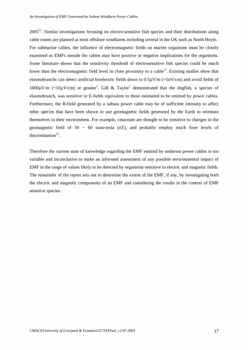
3.1.2 Eddy current field solver model
The eddy current field solver model simulates the effects of time-varying currents in parallel-
conductor structures. It can be used to model eddy currents, skin effects and magnetic flux. In
addition, any quantity that can be derived from the basic B-field quantities can be analysed. The eddy
current field solver computes the magnetic vector potential, from which the B-field ( )H t , the
magnetic flux density ( )B t and the current density ( )J t can be derived.
The eddy current field solver calculates the eddy currents by solving the magnetic and electric
potentials in the following equation:
( ) ( )( )1 A Aj j∇× ∇× = + − − ∇σ ωε ω φµ
(4)
where A is the magnetic vector potential and µ is the permeability. All object interfaces are defined
as natural boundaries, i.e., the tangential component of H and the normal component of B are
continuous across the object surface, according to the following relationships:
1 2H H Jt t s= + (5)
1 2B Bn n= (6)
where H t is the B-field strength tangential to the interface, B n is the magnetic flux density normal to
the interface, and J s is the surface current density.
An Investigation of EMF Generated by Subsea Windfarm Power Cables
CMACS/University of Liverpool & Econnect/J2733/Final_v1/07-2003 21
3.2 MODELLING OF THE CABLE
3.2.1 Geometrical modelling of the problem
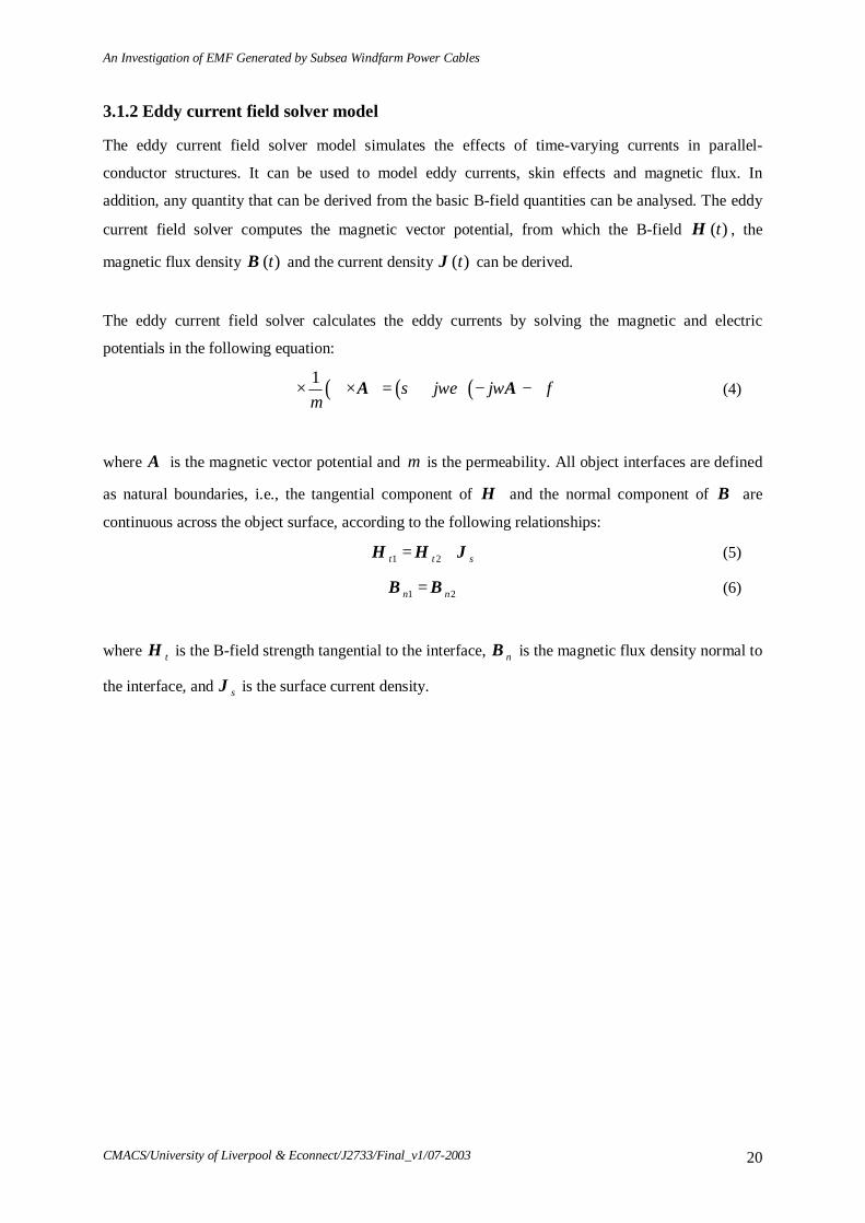
Figure 3.1 shows the constructional geometry of the Pirelli 132kV XLPE submarine cable (ie. the
cable components and positional relationships between them) given in its specification whilst Figure
3.2 shows the simplified geometry of the cable that was simulated in the Maxwell 2D software
package. Dimensions of each section in the simulated cable model were identical to those of the real
cable. The diameter of the cable is 18cm and consists of a triangular symmetrical arrangement of three
single-core sub-cables, where the sub-cables are laid as at the corners of an equilateral triangle. Every
core in the three-phase cable, comprising phases 1, 2 and 3 with 120° phase shift from each other, can
be regarded as a return line of the two others. In each core, the lead sheath serves as a conducting
screen to confine the E-field radial inside each sub-cable. Outer steel armouring provides stronger
mechanical strength and added protection to the cable. Inside each core is filled with polyethylene
XLPE, which has good electrical and thermal performance.
For the simulation of the submarine cable working in a real environment, we set up the simulation
scenario where the submarine cable was buried in the seabed to a depth of 1 m beneath the seabed
surface. Figure 3.3 shows the simulation scenario, with the cable laid perpendicular to the plane of the
paper and its cross-section modelled as shown in Figure 3.2.
Figure 3.1: Constructional geometry of the Pirelli 132kV XLPE submarine cable
An Investigation of EMF Generated by Subsea Windfarm Power Cables
CMACS/University of Liverpool & Econnect/J2733/Final_v1/07-2003 22
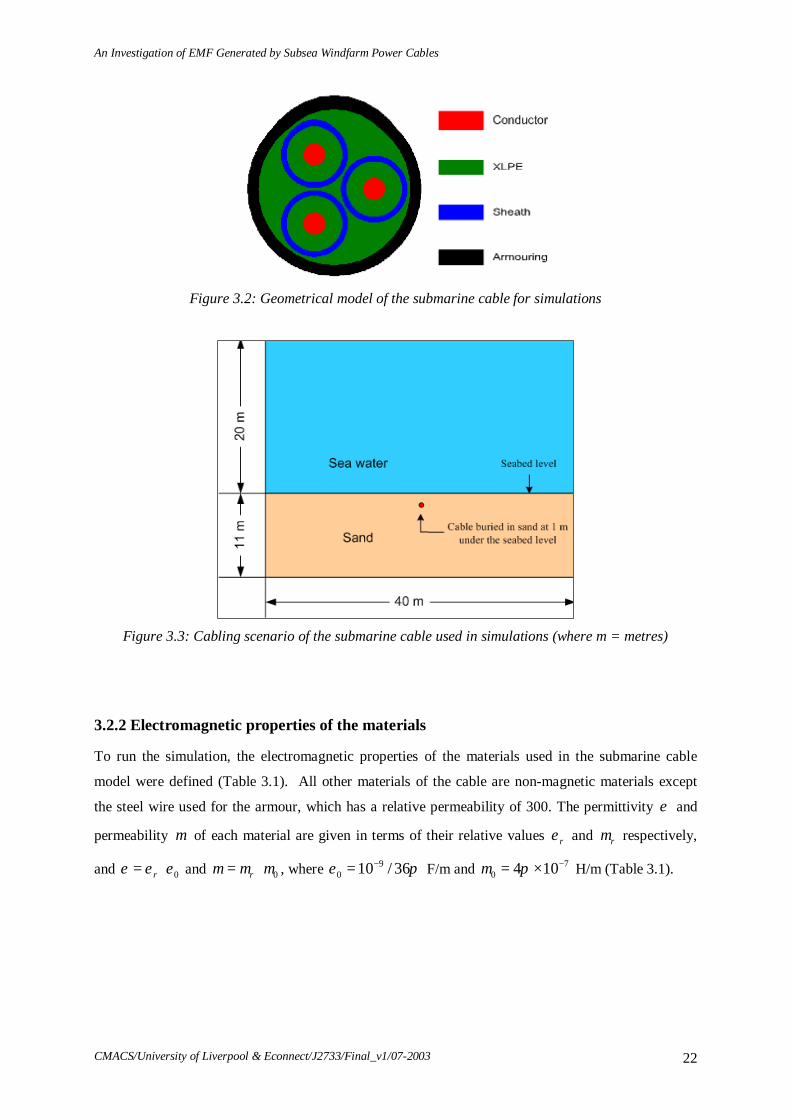
Figure 3.2: Geometrical model of the submarine cable for simulations
Figure 3.3: Cabling scenario of the submarine cable used in simulations (where m = metres)
3.2.2 Electromagnetic properties of the materials
To run the simulation, the electromagnetic properties of the materials used in the submarine cable
model were defined (Table 3.1). All other materials of the cable are non-magnetic materials except
the steel wire used for the armour, which has a relative permeability of 300. The permittivity ε and
permeability µ of each material are given in terms of their relative values rε and rµ respectively,
and 0r= ⋅ε ε ε and 0r= ⋅µ µ µ , where 90 10 / 36−=ε π F/m and 7
0 4 10−= ×µ π H/m (Table 3.1).

An Investigation of EMF Generated by Subsea Windfarm Power Cables
CMACS/University of Liverpool & Econnect/J2733/Final_v1/07-2003 23
Table 3.1 Electromagnetic properties of the materials of the submarine cable.
Permittivity
er
Conductivity
σ (s/m)
Permeability
rµ
Conductor (Copper) 1.0 58, 000, 000 1.0
XLPE 2.5 0.0 1.0
Sheath (Lead) 1.0 5, 000, 000 1.0
Armour (Steel wire) 1.0 1,100, 000 300
Seawater 81 5.0 1.0
Sea sand 25 1.0 1.0
In the model the cable operated at 50 Hz (UK mains power frequency) with AC voltage of 132 kV
between phases and AC current of 350A flowing in each conductor. With information on the
geometry, electromagnetic properties of the cable and the excitation sources, the Maxwell 2D software
computed the electromagnetic fields in the model.

An Investigation of EMF Generated by Subsea Windfarm Power Cables
CMACS/University of Liverpool & Econnect/J2733/Final_v1/07-2003 24
3.3 SIMULATION RESULTS AND DISCUSSION
3.3.1 EMF generated by a cable with perfect shielding
3.3.1.1 AC Conduction field solver model
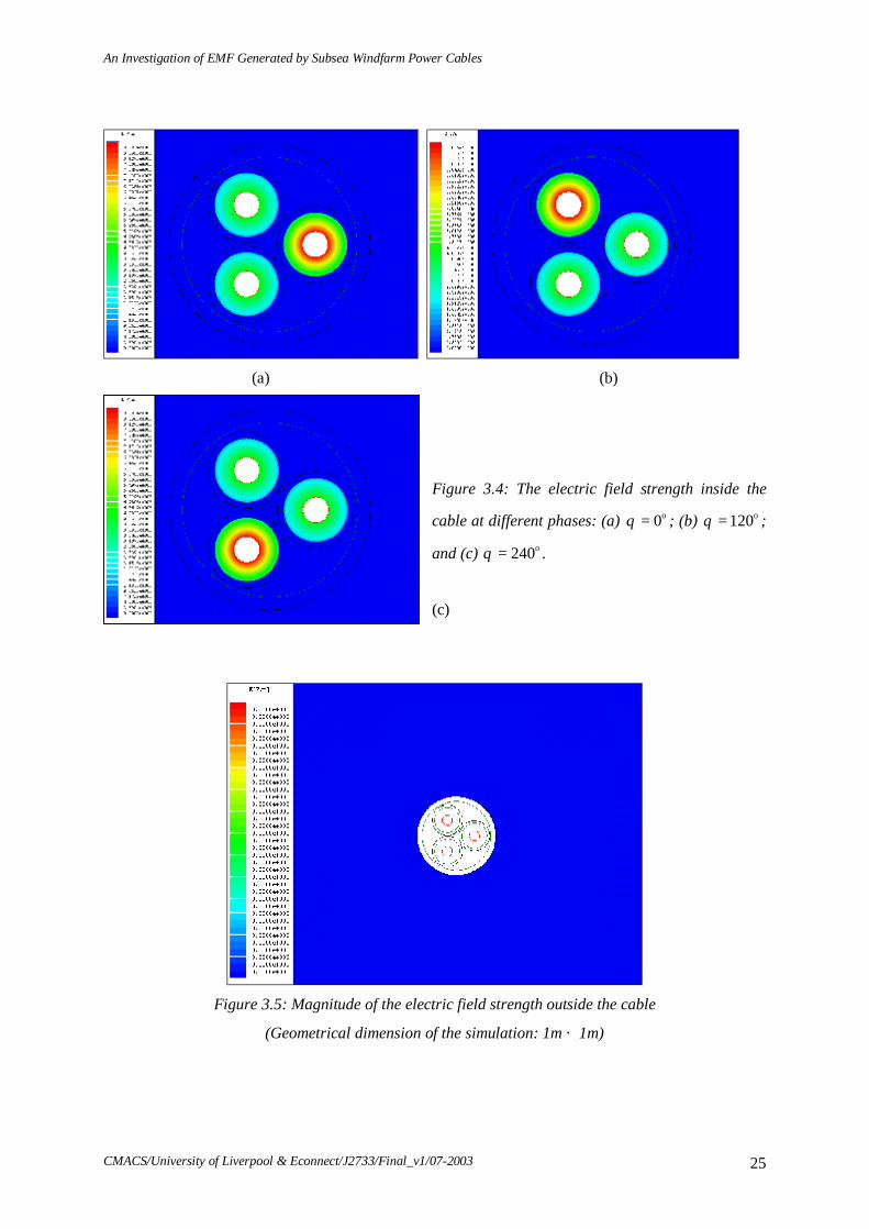
By assigning the time-varying voltage source to each conductor of the three-core cable, the E-field
distributions were obtained using the AC Conduction Field Solver model. Figure 3.4 shows the
simulated E-field strength inside all cores of the cable at different phases. Owing to the alternating
voltage sources with a 120° phase shift at each core, the E-field inside each core alternately attains the
maximum value (Figure 3.4). Metallic sheaths in the cable create earthed shields for all cores, so the
E-fields are seento be strictly confined in each core (Figure 3.4) and have a radially symmetric
distribution within the dielectric XLPE. Consequently, no E-field is leaked from each core, giving rise
to no E-field outside the submarine cable, as shown in Figure 3.5.
The simulation results shown in Figures 3.4 and 3.5 are for ideal cases where the sheaths of the cable
are 'perfectly' earthed.
Whilst the simulation shows that a perfectly shielded cable would effectively confine E-fields within
each core, induced E-fields outside of the submarine cable may still be generated. Maxwell’s
equations tell us that alternating E-fields generate B-fields, which in turn generate induced E-fields.
This is a result of the fact that AC currents flowing in each conductor of the cable generates changing
B-fields around the conductor. This changing B-field 'induces' an E-field in the surrounding medium
and eddy currents in the three conductors. These effects cannot be simulated with the AC Conduction
Field Solver, but are considered in the next section.
Summary
The following points can be drawn in summary:
• Maxwell's AC Conduction Field Solver Model was used to investigate whether a 132kV
XLPE submarine cable generates E-fields. This model assumed that the cable was perfectly
shielded.
• The E-field results are scalable to other voltages. For example, the scaling factor for applying
33kV to the cable is 0.25 (i.e. 33,000/132,000).
• The model showed that the cable did not directly generate an E-field outside the cable.
• B-fields generated by the cable (modelled in Section 3.3.1.2), will however generate 'induced'
E-fields outside the cable.
• This model could not quantify induced E-fields.
An Investigation of EMF Generated by Subsea Windfarm Power Cables
CMACS/University of Liverpool & Econnect/J2733/Final_v1/07-2003 25
(a) (b)
Figure 3.4: The electric field strength inside the
cable at different phases: (a) 0= oθ ; (b) 120= oθ ;
and (c) 240= oθ .
(c)
Figure 3.5: Magnitude of the electric field strength outside the cable
(Geometrical dimension of the simulation: 1m × 1m)

An Investigation of EMF Generated by Subsea Windfarm Power Cables
CMACS/University of Liverpool & Econnect/J2733/Final_v1/07-2003 26
3.3.1.2 Eddy current field solver model
An operational submarine cable will have alternating currents flowing in each conductor with a 120°
phase shift at each core. This will generate changing B-fields around each conductor. Figure 3.6 shows
the simulated B-fields inside the cable at different phases. It can be seen that the B-fields have a
temporal rotation along the axis of the cable (Fig 3.6).
The sheaths of the cable can provide good shielding of the E-field, as discussed in Section 3.3.1.1 and
shown in Figure 3.4, however, the sheaths cannot shield B-fields due to AC flowing in the cable. As a
result of this, B-fields are expected to exist outside the cable.
(a) (b)
(c)
Figure 3.6: The magnetic field strength inside the
cable at different phases: (a) o0=θ ; (b) o120=θ ;
and (c) o240=θ
Figure 3.7 shows the simulated magnitude of magnetic flux density outside the cable with the cable
buried 1m below the seabed. The dimensions of the problem simulated are given in Figure 3.3.
It is clearly seen that strong magnetic fields are present in close proximity to the cable and that these
fields dissipate along the radial direction of the cross-section of the cable (Figure 3.7). It is worth
noting that the B-fields at the same distance to the cable are identical, whether the observation point is
in the seawater or in the sea sand. Continuous B-fields are present across the boundary between the

An Investigation of EMF Generated by Subsea Windfarm Power Cables
CMACS/University of Liverpool & Econnect/J2733/Final_v1/07-2003 27
seawater and the sea sand as neither seawater or sea sand have magnetic properties i.e. the sediment
type in which a cable is buried has no effect on the magnitude of B-field generated.
The magnitude of the B-field on the ‘skin’ of the cable (i.e. within millimetres) is approximately
1.6μT. As a result of using 50Hz AC, this B-field will vary predictably with time and will be
superimposed onto any existing B-field (eg. the Earth's geomagnetic field which has a strength of
approximately 50µT). The strength of the B-field associated with the cable diminishes rapidly and in a
non-linear manner with distance and background levels are reached within 20m (Figure 3.7). The
maximum B-field strength of 1.6μT corresponds well with the B-field strength calculated by AEI
Cables Ltd4 of 1.45μT for a power cable carrying a similar current.
Figure 3.7: Magnitude of the magnetic flux density outside the cable
(Geometrical dimension of the simulation is as given in Figure 3.3)
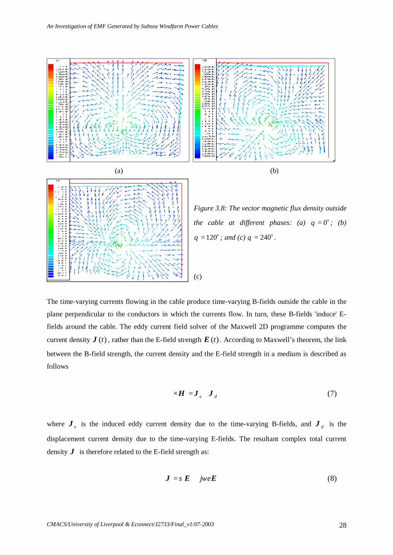
Figure 3.8 shows the vector view of the magnetic flux density outside the cable at different phases. In
contrast to the case of a cable with a single-core, the B-fields around the three-phase cable are no
longer concentric to the axis of the cable and are not uniformly circular. This is a result of a specific
phase of the current flowing in each conductor is different from that in the two others.
An Investigation of EMF Generated by Subsea Windfarm Power Cables
CMACS/University of Liverpool & Econnect/J2733/Final_v1/07-2003 28
(a) (b)
Figure 3.8: The vector magnetic flux density outside
the cable at different phases: (a) 0= oθ ; (b)
120= oθ ; and (c) 240= oθ .
(c)
The time-varying currents flowing in the cable produce time-varying B-fields outside the cable in the
plane perpendicular to the conductors in which the currents flow. In turn, these B-fields 'induce' E-
fields around the cable. The eddy current field solver of the Maxwell 2D programme computes the
current density ( )J t , rather than the E-field strength ( )E t . According to Maxwell’s theorem, the link
between the B-field strength, the current density and the E-field strength in a medium is described as
follows
H J Je d∇× = + (7)
where J e is the induced eddy current density due to the time-varying B-fields, and J d is the
displacement current density due to the time-varying E-fields. The resultant complex total current
density J is therefore related to the E-field strength as:
J E Ej= +σ ωε (8)

An Investigation of EMF Generated by Subsea Windfarm Power Cables
CMACS/University of Liverpool & Econnect/J2733/Final_v1/07-2003 29
Figure 3.9 shows the simulated current density in both the seawater and the sea sand. Since the
seawater and the sea sand have different electrical properties (see Table 3.1) with different
conductivity values, the simulated current density is discontinuous across the boundary between the
seawater and the sea sand. Due to the higher conductivity and permittivity of seawater, the current
density at an observation point in the seawater is higher than that in the sea sand, both at the same
distance to the cable.
Figure 3.9: Magnitude of the current density outside the cable
(Geometrical dimension of the simulation is as given in Figure 3.3)
The magnitude of the current density on the ‘skin’ of the cable (i.e. within millimetres) and on the
seabed directly above the cable is 0.000365A/m2. Using Equation (8), this can be approximated to E-
field strength of 91.25μV/m (assuming a seawater conductivity of 4 Siemens per metre [S/m] ie. fully
marine). The E-field in the seabed dissipates rapidly to only 1 or 2 μV/m within a distance of
approximately 8m from the cable. At the same distance in the seawater however, the E-field strength is
approximately 10μV/m (=0.1 μV/cm).
Hence, the induced current densities are effectively the same on the “skin” of the cable and on the
seabed, therefore the mitigation effects of burying the cable one metre into the seabed are negligible
from an electromagnetic view. The induced current density in the seawater decreases with distance
from the cable and there is a more rapid reduction within the sediment (see Figure 3.9). The linkage
between the induced current and E-field is defined by Equation (8).
Gill and Taylor1 determined through a literature review and experimentation that dogfish were
attracted to E-fields ranging from 0.5μV/m - 10μV/m, whereas they avoided fields of 1000μV/m.

An Investigation of EMF Generated by Subsea Windfarm Power Cables
CMACS/University of Liverpool & Econnect/J2733/Final_v1/07-2003 30
Therefore, a dogfish (or another species with similar sensitivity) may be able to detect a buried cable
within a number of metres of the cable (horizontally along the seabed or vertically in the water
column).
The simulation has been conducted using a three-phase cable, characteristic of UK windfarm cabling
proposals, and is different from a single-core cable modelled at Horns Rev. As such, direct comparison
of the results presented above with the results of modelling for Horns Rev is not possible at this stage.
Summary
The following points can be made in summary:
• Maxwell's Eddy Current Field Solver model was used to investigate B-field generated by a
132kV XLPE submarine cable. This model assumed that the cable was perfectly shielded.
• The results of the simulation showed that B-fields are present in close proximity to the cable and
that any non-magnetic sediment type in which a cable is buried has no effect on the magnitude of
B-field generated.
• The magnitude of the B-field on the ‘skin’ of the cable (i.e. within millimetres) is approximately
1.6μT which will be superimposed on any other B-fields (eg. earth’s geomagnetic field).
• The magnitude of the B-field associated with the cable falls to background levels within 20m.
• An induced E-field is generated by the B-field, irrespective of shielding.
• The induced E-field in the seawater decreases with distance from the cable and there is a
more rapid reduction within the sediment
• The strength of the induced E-field is within the sensitivity range of dogfish.
An Investigation of EMF Generated by Subsea Windfarm Power Cables
CMACS/University of Liverpool & Econnect/J2733/Final_v1/07-2003 31
3.3.2 EMF generated by cables with non-perfect shielding
In section 3.3.1, it is shown that the E-field would be strictly confined within each core of the cable
due to the perfect shielding of the conductor screen, i.e., the sheath of each core is well earthed and the
potential of the sheath is zero.
In this section, the model simulates the situation where the conductor-shielding screen is not well
earthed and thus, the potential of the cable sheath is not zero. A reference circular boundary with zero
potential at 10m away from the axis of the cable was defined. Seawater was modelled as the medium
between the cable and the reference boundary. Due to the precision limitation of the software,
Maxwell 2D's AC conduction field solver model could only simulate the model with the conductivity
of the sheath of up to 3000 S/m.
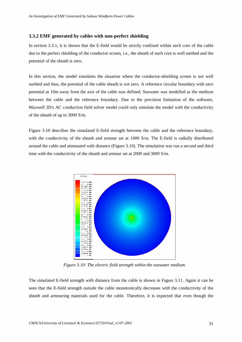
Figure 3.10 describes the simulated E-field strength between the cable and the reference boundary,
with the conductivity of the sheath and armour set at 1000 S/m. The E-field is radially distributed
around the cable and attenuated with distance (Figure 3.10). The simulation was run a second and third
time with the conductivity of the sheath and armour set at 2000 and 3000 S/m.
Figure 3.10: The electric field strength within the seawater medium.
The simulated E-field strength with distance from the cable is shown in Figure 3.11. Again it can be
seen that the E-field strength outside the cable monotonically decreases with the conductivity of the
sheath and armouring materials used for the cable. Therefore, it is expected that even though the

An Investigation of EMF Generated by Subsea Windfarm Power Cables
CMACS/University of Liverpool & Econnect/J2733/Final_v1/07-2003 32
sheath and armour are not well earthed, the E-field strength at or above 1m distance from the cable is
very small for high conductive sheath and armouring materials.
Figure 3.11: The electric field strength outside the cable for different conductivity values
Summary
The following points can be made in summary:
• An E-field would be generated outside a cable owing to non-perfect shielding/earth.
• This additional E-field is smaller than the normal induced E-field and decreases with the
distance from the cable. It is not considered additive to any existing E-field.
• Burying the cable one metre deep would reduce the emitted E-field at the seabed.
An Investigation of EMF Generated by Subsea Windfarm Power Cables
CMACS/University of Liverpool & Econnect/J2733/Final_v1/07-2003 33
3.4 CONCLUSIONS FROM MODELLING EMF WITH AND WITHOUT PERFECT
CABLE SHIELDING
The Maxwell 2D programme was used to investigate EMF generated by 132kV XLPE three-phase
submarine cable with an AC current of 350A through the application of two models; the AC
Conduction Field Solver and the Eddie Current Field Solver.
The results of simulations showed that a cable with perfect shielding i.e. where conductor sheathes are
grounded, does not generate an E-field directly. However, a B-field is generated in the local
environment by the alternating current in the cable. This in turn, generates an induced E-field close to
the cable within the range detectable by electro-sensitive fish species. The induced E-field is related to
the current in the cable. A smaller current would proportionally produce a lower induced E-field, i.e. a
cable current of 175A will give rise to half the induced current density at 350A and therefore half the
induced E-field.
Simulations of a 132kV XLPE three-phase submarine cable with non-perfect shielding, i.e. where
there is poor grounding of sheathes showed that there is a leakage E-field (not induced), but it is
smaller than the induced E-fields. Again if the cable were operated at a lower voltage the electrical
field results would need to be scaled. e.g. for a 33kV cable the scaling factor is 0.25.

An Investigation of EMF Generated by Subsea Windfarm Power Cables
CMACS/University of Liverpool & Econnect/J2733/Final_v1/07-2003 34
4. MEASURING EMF IN THE ENVIRONMENT
4.1 INTRODUCTION
To directly measure the electromagnetic emission from undersea cables two sensors were developed,
one able to detect B-fields and the other E-fields when placed near to a three-phase AC power cable in
seawater. These sensors are briefly described in this section and circuits included in Appendix II.
The sensors were tested and calibrated in the laboratory, first at the bench and then in a seawater tank.
In situ site trials were then undertaken at Rhyl in the Clwyd Estuary.
4.2 DESIGNING THE MAGNETIC AND ELECTRIC FIELD SENSORS
4.2.1 The Magnetic field sensor
Hall effect and the Fluxgate sensors are commonly used to measure magnetic fields of around 100 μT
and 14 nT respectively. They are capable of measuring fields over a wide range of frequencies from 0
Hz (DC) to several 1000 Hz. Both are able to measure non-varying signals which means that they are
used to detect the earth’s B-field (≈50 μT), or the field from high voltage direct current links (HVDC)
Since the primary interest was in the mains power frequency (50 Hz) an alternative design based on a
search coil was used. In a search coil varying B-fields produce a voltage that is proportional to the B-
field. A differential electronic amplifier provided gain thereby increasing the B-field sensitivity of the
sensor, while also reducing its sensitivity to E-fields.
The system was calibrated using a 70 nT RMS field generated from a 600 mm diameter coil.
Experiments performed on site indicated that the unit had a minimum sensitivity of 0.5 nT RMS.
The sensor proved reliable but needed to be held stationary to prevent pick-up from the earth’s B-field,
which can interfere with readings. This pick-up could be reduced and the sensitivity increased further
by the addition of a band-pass filter.
4.2.2 The Electric field sensor
Detecting very low electric fields within the range that electro-receptive fish are sensitive to required a
sensing system able to detect fields of around 1 to 10 μV/m. Two E-field sensors were developed:
• A high input impedance electric field sensor
• A low input impedance electric field sensor

An Investigation of EMF Generated by Subsea Windfarm Power Cables
CMACS/University of Liverpool & Econnect/J2733/Final_v1/07-2003 35
4.2.2.1. The High input impedance electric field sensor
Electrodes in contact with water generate a relatively large electrode voltage of approximately 200
mV. This varies by a few 1000 μV with the salinity and also with temperature (approximately 1000
μV/˚C). Electrode voltage variations that occur at the mains power frequency may be perceived as
being due to effects from the mains power-line. In order to prevent this an E-field sensor with a high
input impedance was developed.
To separate the electrode from the seawater a 1-mm thick epoxy layer was used which acted as a
capacitor coupling the signals from the seawater to the 4-cm² electrode without producing an electrode
voltage. The epoxy layer used had a capacitance of approximately 12 pF which was smaller than that
of other sensors that have been developed. One problem that resulted was this produced a large
amplifier input current noise which limited the sensitivity of the sensor system. Therefore, the
resulting noise limited the minimum detectable E-field from a 100 mm long sensor to 155 μV/m.
Furthermore, the sensor was sensitive to vibration and also needed time to recover following exposure
to voltages exceeding a few millivolts.
4.2.2.2. The Low input impedance electric field sensor
A low impedance sensor was then developed that works in a similar way to a fish ampullary electro-
receptor system.
The low impedance E-field sensor used 3 cm² lead electrodes 10-cm apart. Lead has a very low
electrode-to-electrode voltage and so minimised any electrode noise. The electrodes were polarisable
meaning they did not react chemically with the water, instead charge would have built up on the
surface of these electrodes, thereby acting like a capacitor (with a capacitance of around 100 μF per
cm²). The DC current flowing through the electrodes had to be low (around 1 μA), hence low leakage
capacitors were used to connect the electrodes to the rest of the circuit.
The sensor head (Figure 4.1), was made symmetrical to minimise the cross-sensitivity to B-fields
when immersed in water. The head (enclosed in thin foil) and sensor electronics were tested and found
to have a negligible B-field sensitivity (less than 10 μV/m in a 5000 nT field).

An Investigation of EMF Generated by Subsea Windfarm Power Cables
CMACS/University of Liverpool & Econnect/J2733/Final_v1/07-2003 36
Figure 4.1: Low input impedance electric field sensor system
The sensor head was connected to the electronics by a short-shielded lead (Figure 4.1). The sensor
electronics amplified the voltage before it was transmitted to the measurement equipment using a fibre
optic cable. This arrangement ensured that the B-fields and ground loops did not interfere with the
measurement process. The electronics of the systems would only sense signals as low as 0.42 μV RMS
at 50 Hz. This gave the 100 mm long sensor a minimum detectable E-field of 4.2 μV/m RMS.
To calibrate the sensor it was placed in an aluminium enclosure then connected to a signal generator
via a 100 dB attenuator.

An Investigation of EMF Generated by Subsea Windfarm Power Cables
CMACS/University of Liverpool & Econnect/J2733/Final_v1/07-2003 37
4.3 LABORATORY TESTING
Prior to site trials at Rhyl a number or experiments were performed in a 46 cm wide x 26 cm deep x 90
cm long tank.
Initially the tank was filled with tap water (with a conductivity of 0.17 milli-siemens/cm) and a
standard household 3-core mains electricity cable (with no screen or armour) placed in it. With the
cable connected to a 120 VRMS voltage, and with no current flowing, the high-impedance E-field sensor
was able to detect a field of 2200 μV/m RMS close to the cable but was unable to detect low E-fields of
a few hundred µV/m RMS .
The low impedance sensor was then tested in the water filled tank with added sea salt to a
concentration of 33 g/Litre (conductivity 45 milli-siemens/cm). With the cable connected a 240 V RMS
voltage, and with no current flowing, the E-field 100 mm from the cable was 25 μV/m RMS.
A mock cable was then constructed to mimic some of the characteristics of an undersea power-line. Its
cross-section is shown in Figure 4.2.
Figure 4.2 Cross section of the mock cable
The mock cable was connected to a 240 V RMS voltage with no current flowing and the E-field was
measured parallel to the conductor in the surrounding seawater at three set distances (Figure 4.3).
These levels were probably higher than would occur with a real cable as the thin foil shield used
would not be as effective at reducing E-field emission as the sheath and armour on a real cable.
However this higher than expect field could be compensated by the lower voltage used for the test
(200 V RMS rather than 11/33 kV RMS).

An Investigation of EMF Generated by Subsea Windfarm Power Cables
CMACS/University of Liverpool & Econnect/J2733/Final_v1/07-2003 38
Figure 4.3 Electric field near the mock cable carrying a voltage
The connections were altered to carry a 50 Hz current of just 0.5 ARMS; this was approximately 0.2%
of the current likely to be carried by a real cable. The voltage difference between the send and the
return ends of the conductors was negligible (0.5 VRMS). The B-field measured around the mock cable
was large (shown in Figure 4.4). The B-field was higher than would occur with a real cable carrying
0.5 ARMS since the mock cable had no outer armour to reduce B-field emission, however a real cable
would carry a far higher current.
Figure 4.4 Magnetic field near the mock cable carrying a current
The low-impedance E-field sensor was then used to detect the E-field that was induced in the seawater
tank by the time varying B-field produced by electric current flowing in the cable. The induced E-field
measured is shown in Figure 4.5.

An Investigation of EMF Generated by Subsea Windfarm Power Cables
CMACS/University of Liverpool & Econnect/J2733/Final_v1/07-2003 39
Figure 4.5 Induced electric field the near mock cable carrying a current
Unlike the high impedance E-field sensor, the low impedance sensor recovered immediately from
exposure to large E-fields.
The laboratory measurements of electric and B-fields agreed with the values expected from
calculations.

An Investigation of EMF Generated by Subsea Windfarm Power Cables
CMACS/University of Liverpool & Econnect/J2733/Final_v1/07-2003 40
4.4 FIELD TESTING
4.4.1 Introduction
Site trials were undertaken to test the magnetic and E-field sensors and evaluate the levels of magnetic
and E-field emission from a real cable in situ. The aim of this investigation was to determine the
following:
• Whether the sensors built could measure and detect electric and magnetic fields in a marine
environment, and
• How these fields compared with the predictions of the modelling (Section 3).
Measurements were taken in the vicinity of power cables crossing the Clwyd Estuary at Rhyl, North
Wales. This site was selected for the following reasons:
• The presence of a 33kV and an 11kV underwater cables
• Proximity to Liverpool if repeat measurements were required due to complications
• Site access and personal knowledge of the environment.
Figure 4.6 shows the location of the two cables running across the estuary upstream of the nearby
Foryd Bridge (A494). Both cables lie approximately 1m below the surface of marine muddy sand.
The 33 kV three-phase cable carried 50ARMS per phase. The cable has a metalised foil sheath
surrounding each conductor. An outer lead sheath enclosed all three phases separated from the foil
screens by paper insulation and the armour was provided as steel wire. The cable conforms to the
British Standard BS-6480.
The 11 kV three-phase cable carried 60 ARMS per phase. Each of the three phases was sheathed. An
outer corrugated aluminium sheath enclosed all three phases and the cable conforms to the Electricity
Association Technical Specification EATS 09-12.
4.4.2 Methodology
The electric and magnetic fields were measured with the sensors at the following radial distances
upstream from each cable: 0m (i.e. directly above the cable), 1m, 2m, 5m, 10m, 20m and 400m. Note:
the low impedance E-field sensor was adjusted to cover the range 6 to 100 μV/m RMS.
The average of the sensor readings taken over a 10 second interval was recorded with the sensors
submerged to a depth of approximately 1.5m below the surface of the water on an incoming tide.
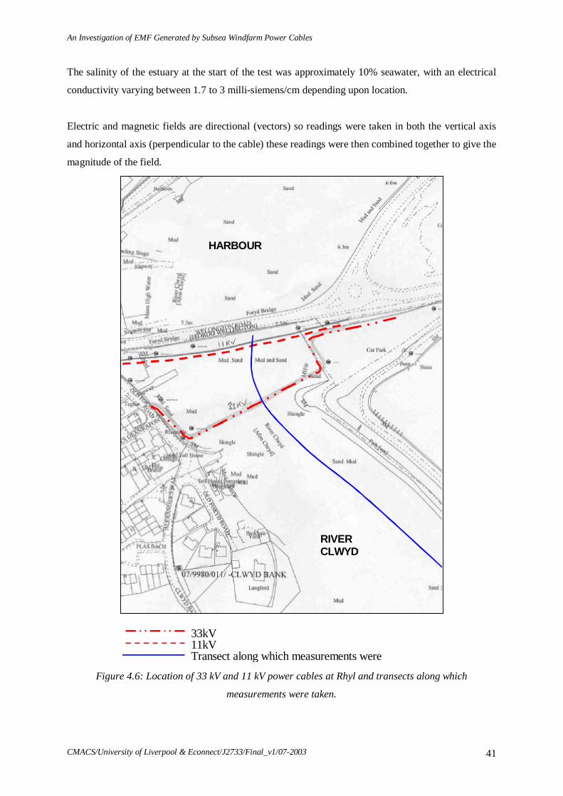
An Investigation of EMF Generated by Subsea Windfarm Power Cables
CMACS/University of Liverpool & Econnect/J2733/Final_v1/07-2003 41
The salinity of the estuary at the start of the test was approximately 10% seawater, with an electrical
conductivity varying between 1.7 to 3 milli-siemens/cm depending upon location.
Electric and magnetic fields are directional (vectors) so readings were taken in both the vertical axis
and horizontal axis (perpendicular to the cable) these readings were then combined together to give the
magnitude of the field.
33kV 11kV Transect along which measurements were
RIVER CLWYD
HARBOUR
Figure 4.6: Location of 33 kV and 11 kV power cables at Rhyl and transects along which
measurements were taken.

An Investigation of EMF Generated by Subsea Windfarm Power Cables
CMACS/University of Liverpool & Econnect/J2733/Final_v1/07-2003 42
4.5 RESULTS
4.5.1 Magnetic field sensor
Near the 33 kV cable the magnetic field was measured as 50 nT RMS orientated 56˚ from vertical. The
field decreased with distance from the cable axis (Figure 4.7). The orientation of the field beyond 5m
was approximately 0˚ from vertical and at 400 metres from the cable the sensor picked up only noise
(0.5 nT RMS)
Magnetic field near the 33 kV cable
0
10
20
30
40
50
60
0 5 10 15 20Distance / metres
Fie
ld /n
T R
MS
Figure 4.7 Magnetic field near the 33 kV cable
The position of the 11 kV cable was not precisely known, due to lack of markers, however it was
located using the B-field sensor. Figure 4.8 shows the measured B-field; the negative distance readings
were limited by the A494 Bridge and movement further than 15m in the positive direction would have
led to interference from the 33 kV cable. The field from the 11 kV cable appeared to be more widely
distributed than the 33 kV cable which may have been a consequence of the individually sheathed
conductors.
Magnetic field near the 11 kV cable
0
102030
405060
-10 -5 0 5 10 15Distance / metres
Fiel
d / n
T R
MS
Figure 4.8 Magnetic field near the 11 kV cable
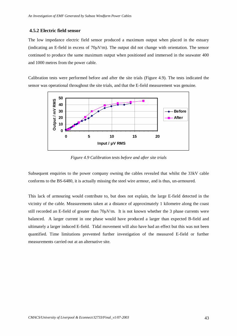
An Investigation of EMF Generated by Subsea Windfarm Power Cables
CMACS/University of Liverpool & Econnect/J2733/Final_v1/07-2003 43
4.5.2 Electric field sensor
The low impedance electric field sensor produced a maximum output when placed in the estuary
(indicating an E-field in excess of 70μV/m). The output did not change with orientation. The sensor
continued to produce the same maximum output when positioned and immersed in the seawater 400
and 1000 metres from the power cable.
Calibration tests were performed before and after the site trials (Figure 4.9). The tests indicated the
sensor was operational throughout the site trials, and that the E-field measurement was genuine.
01020304050
0 5 10 15 20Input / µV RMS
Out
put /
mV
RMS
BeforeAfter
Figure 4.9 Calibration tests before and after site trials
Subsequent enquiries to the power company owning the cables revealed that whilst the 33kV cable
conforms to the BS-6480, it is actually missing the steel wire armour, and is thus, un-armoured.
This lack of armouring would contribute to, but does not explain, the large E-field detected in the
vicinity of the cable. Measurements taken at a distance of approximately 1 kilometre along the coast
still recorded an E-field of greater than 70μV/m. It is not known whether the 3 phase currents were
balanced. A larger current in one phase would have produced a larger than expected B-field and
ultimately a larger induced E-field. Tidal movement will also have had an effect but this was not been
quantified. Time limitations prevented further investigation of the measured E-field or further
measurements carried out at an alternative site.

An Investigation of EMF Generated by Subsea Windfarm Power Cables
CMACS/University of Liverpool & Econnect/J2733/Final_v1/07-2003 44
4.6 METHODOLOGY FOR CALCULATION OF EMF
A method is given below for calculating the induced E-field around a low frequency (such as 50 Hz)
AC power cable due to the emanating B-field. This method does not consider E-fields generated as a
result of non-perfect shielding or induced E-fields generated by movement of water through the B-
field generated. Furthermore, this method requires in situ measurement of the B-field generated by an
operational cable.
A number of factors can influence the measured B-field; therefore the field should be measured at
various distances using apparatus such as that developed and reported in section 4, or by using a
commercial magnetometer with sufficient sensitivity. Tests need to be performed several hundred
metres from other cables or electrical equipment and care taken to ensure the B-field recorded is not
emanating from the current supply apparatus or load at either end of the cable. The magnetometer
should be orientated to give a maximum reading. Furthermore, measurements should be taken with the
magnetometer at a depth of 0.5 to 1m of seawater directly over the cable.
The B-field measurable near a power-line (carrying an electric current) can be approximately related
to an induced E-field in the surrounding medium (eg. the seawater) by the following equations:
Electric Field (V/m) ≈ 2 * π * Power frequency (Hz) * Magnetic Flex Density (T) Or Electric Field (μV/m) ≈ 2,000 * π * Power frequency (Hz) * Magnetic Flex
Density (nT) Where The power frequency used in the UK is 50 Hz.
This can also be related to the electric current density in water using the equation: Current Density (A/m²) = Electric Field (V/m) * Conductivity (S/m) Or Current Density (A/m²) = Electric Field (μV/m) * Conductivity (mS/cm)/10,000,000 Where: Conductivity of Freshwater ≈ 0.025 Siemens/m (S/m) = 0.25 milli-Siemens/cm (mS/cm) Conductivity of Sea water ≈ 4 Siemens/m (S/m) = 40 milli-Siemens/cm (mS/cm)

An Investigation of EMF Generated by Subsea Windfarm Power Cables
CMACS/University of Liverpool & Econnect/J2733/Final_v1/07-2003 45
4.7 CONCLUSIONS DRAWN FROM MEASURING EMF
The following points can be drawn in conclusions:
• Both magnetic and electric fields were detected.
• The B-field sensor developed performed well in the laboratory and site trials. It was able to detect
B-fields down to 0.5 nT RMS.
• The B-field level measured during site trials (56 nT RMS ) closely matched levels predicted by
modelling (Section 3). This validates the model used for B-field calculations.
• Tests in the seawater tank in the laboratory showed that the E-field measured does not vary
significantly with the shape of the sensor. This result implies the E-field in the water can be
calculated from the current density using the following equation:
Electric field (μV/m) = 1000000 • Current density (A/m²)
Conductivity (siemens/m)
= 10000 • Current density (mA/m²)
Conductivity (milli-siemens/cm)
(For seawater the salinity/conductivity is approximately 4 S/m or 40 mS/cm)
• The modelling (Section 3) predicted that the B-field observed during field trials would induce an
electric current density in the seawater of 0.1 mA/m² with a cable buried to a depth of 1m. It
therefore follows from the above conclusion that the induced E-field in the water would be around
25 μV/m.
• Tests performed on a mock power cable indicated that with no armour or shield the B-field outside
the cable is very high at approximately 1000 μT RMS. This is a similar level to that predicted for
single-phase power cables12.
• A low input impedance E-field sensor was developed that had sensitivity comparable to that of
electro-sensitive fish. During site trials this sensor detected a large E-field (above 70 μV/m)
sufficient to overdrive the sensor.
• A contributory factor to this field may have been the lack of steel armour in the 33kV cable at
Rhyl. However, this fact does not completely account for the large E-field detected at a distance of
approximately 1 kilometre from the cable. Time limitations did not allow further investigation of
the detected field.

An Investigation of EMF Generated by Subsea Windfarm Power Cables
CMACS/University of Liverpool & Econnect/J2733/Final_v1/07-2003 46
• High input impedance E-field sensors tend to be sensitive to sound; therefore producing a sensor
with sufficient sensitivity for this application (i.e. low output noise) would be difficult and would
require further work.

An Investigation of EMF Generated by Subsea Windfarm Power Cables
CMACS/University of Liverpool & Econnect/J2733/Final_v1/07-2003 47
5. MITIGATION FOR EMF
This section considers mitigation for EMF generated by the present industry standard sub-sea power
cables. Three areas are considered:
• Effects of permeability of the power cable armour
• Effects of conductivity of the cable sheath and armour
• Effects of cable burial to a depth of 1m below the seabed
5.1 EFFECTS OF PERMEABILITY OF THE CABLE ARMOUR
In the manufacturing process of the submarine cable, armouring is usually provided in the form of
steel wires or tapes around the cable2. The purpose of armouring is to enhance the mechanical strength
of the cable. In the simulations carried out in Section 3, steel wires were assumed as the material for
armouring. However, steel tape can also be used as an armouring material, but its permeability is very
different from that of a steel wire. The relative permeability of steel wire is about 300, but that of a
steel tape is about 30002. The strength of B-fields produced by the cable are dependent not only on the
amplitude of current sources, but also on the electromagnetic properties of the materials used for the
cable and thus it is expected that the armouring material will also have effects on the surrounding
electromagnetic field strength.
In this section, the electromagnetic fields outside the cable with different armouring materials have
been simulated. Without changing the conductivity values of the armour and the electromagnetic
parameters of other materials of the cable (see Table 3.1), the model uses different permeability values
for the armour, i.e., 1.0r =µ , 300r =µ , 1000r =µ and 3000r =µ . Figure 5.1 shows the simulated
magnetic flux density in these cases (the field strength scales for each sub-figures (a)-(d) are identical).
The following relationship is apparent; as the permeability of the armour increases the resultant
electromagnetic field strength outside the cable decreases. This can be explained by the fact that with
higher permeability values, the eddy currents induced in the armour and sheaths due to the changing
B-fields become higher and, in turn, give rise to stronger back EMF in the cable. Consequently, the
resultant B-fields in the medium embedding the cable are decreased and so are the E-fields.
The simulation results indicate that using armour materials with higher permeability values can help to
reduce the electromagnetic fields outside the submarine cable (Figure 5.1).

An Investigation of EMF Generated by Subsea Windfarm Power Cables
CMACS/University of Liverpool & Econnect/J2733/Final_v1/07-2003 48
(a) (b)
(c) (d)
Figure 5.1: Magnitudes of the magnetic flux density outside the cable using armouring with different permeability values: (a) 1.0r =µ ; (b) 300r =µ ; (c) 1000r =µ and (d) 3000r =µ
(Geometrical dimension of the simulation is as given in Figure 3.3
Figure 5.2 shows the relationships between simulated magnetic flux density and current density in the
seawater with distance from the cable for armour with the four different permeability values. The
distance is measured as the spatial separation between the observation point and a point at the seabed
level, both being above the cable. One indication given by Figure 5.2 is that the effects of the
armouring material on the magnetic and induced E-fields in the seawater are non-linear. To illustrate
this further, the magnetic flux density and current density measured at 1 m above the seabed level with
respect to the permeability of the armour are shown in Figure 5.3. From the equations given in section
4.7 the induced E-field decreases from approximately 1000μV/m for permeability value 1.0r =µ , to
0.021μV/m for permeability value 3000r =µ .
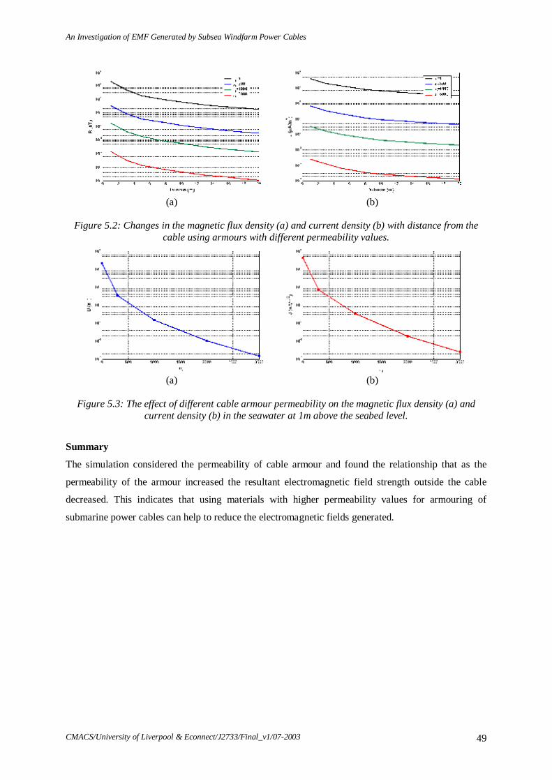
An Investigation of EMF Generated by Subsea Windfarm Power Cables
CMACS/University of Liverpool & Econnect/J2733/Final_v1/07-2003 49
(a) (b)
Figure 5.2: Changes in the magnetic flux density (a) and current density (b) with distance from the
cable using armours with different permeability values.
(a) (b)
Figure 5.3: The effect of different cable armour permeability on the magnetic flux density (a) and
current density (b) in the seawater at 1m above the seabed level. Summary
The simulation considered the permeability of cable armour and found the relationship that as the
permeability of the armour increased the resultant electromagnetic field strength outside the cable
decreased. This indicates that using materials with higher permeability values for armouring of
submarine power cables can help to reduce the electromagnetic fields generated.

An Investigation of EMF Generated by Subsea Windfarm Power Cables
CMACS/University of Liverpool & Econnect/J2733/Final_v1/07-2003 50
5.2. EFFECTS OF CONDUCTIVITY OF THE CABLE SHEATH AND ARMOUR
By analogy to the effects of permeability of the armour on the electromagnetic fields outside the cable,
it is expected that changes in the conductivity values of the sheath and armour will also have an effect.
In this section, the effects of different conductivity values for the sheath and armour on the
surrounding electromagnetic fields have been simulated.
Without changing the permeability values of the armour and sheath and the electromagnetic
parameters of other materials (see Table 3.1), the model uses conductivity values of both the sheath
and armour at 50%, 10% and 1% of the original values listed in Table 3.1. These original values were
referred to reference data and denoted as refσ . Figure 5.4 shows the simulated magnetic flux density
and current density in the seawater in these cases. As the conductivity decreases, the resultant
electromagnetic field strength in the seawater increases (Figure 5.4). This can also be explained by the
fact that with higher conductivity value, stronger back EMF will exist in the cable, consequently the
resultant B-fields are decreased in the seawater and so are the E-fields. The simulation results also
indicate that using materials with higher conductivity values as the sheath and armouring of the cable
can help to reduce the electromagnetic fields outside the submarine cable.
Figure 5.5 shows the simulated magnetic flux density and current density in the seawater for different
electrical sheath and armouring materials at 1m above the seabed level. A clear decreasing, linear
relationship exists between the field strength and the conductivity of the sheath and armour. This is
consistent with the analysis of Voitovich & Kadomskaya 12, who showed that for a close-laid three-
phase cable the longitudinal current density and B-field intensity near the cable are decreased with the
overall conductivity of the shield and armour.
From the equations in section 4.6, the calculated induced E-field decreases from approximately
60μV/m for 1% of refσ , to 17.5μV/m for the reference conductivity ( refσ ).

An Investigation of EMF Generated by Subsea Windfarm Power Cables
CMACS/University of Liverpool & Econnect/J2733/Final_v1/07-2003 51
(a) (b)
(c) (d)
Figure 5.4: Magnitudes of the magnetic flux density outside the cable using the sheath and armour
with different conductivity values (compared to the reference values in Table 3.1): (a) 1%=σ ; (b)
10%=σ ; (c) 50%=σ and (d) 100%=σ .(Geometrical dimension of the simulation is as given in
Figure 3.3)
(a) (b)
Figure 5.5: The changes in magnetic flux density (a) and current density (b) with distance from
the cable using sheaths and armours with different conductivity values.
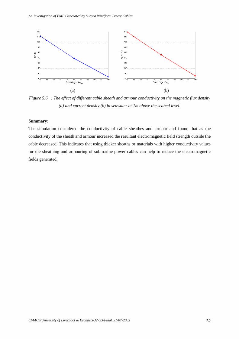
An Investigation of EMF Generated by Subsea Windfarm Power Cables
CMACS/University of Liverpool & Econnect/J2733/Final_v1/07-2003 52
(a) (b)
Figure 5.6. : The effect of different cable sheath and armour conductivity on the magnetic flux density
(a) and current density (b) in seawater at 1m above the seabed level.
Summary:
The simulation considered the conductivity of cable sheathes and armour and found that as the
conductivity of the sheath and armour increased the resultant electromagnetic field strength outside the
cable decreased. This indicates that using thicker sheaths or materials with higher conductivity values
for the sheathing and armouring of submarine power cables can help to reduce the electromagnetic
fields generated.

An Investigation of EMF Generated by Subsea Windfarm Power Cables
CMACS/University of Liverpool & Econnect/J2733/Final_v1/07-2003 53
5.3 EFFECTS OF CABLE BURIAL
The modelling carried out in Section 3, described how a perfectly shielded cable can still generate a B-
field in the local environment and that the B-fields at the same distance to the cable are similar,
whether the observation point is in the seawater or in a non-magnetic seabed. Continuous B-fields are
present across the boundary between the seawater and the sea sand as neither seawater or sea sand
have magnetic properties (see Fig 3.7), i.e. within the parameters of the model the sediment type in
which the cable is buried has no effect on the magnitude of B-field generated as long as the sediment
has non-magnetic properties.
The modelling carried out in Section 3 also identified induced E-fields generated by the B-fields. The
effect of cable burial to 1m on these induced E-fields is apparent in Figure 5.7.
Figure 5.7: Magnitude of the current density outside the cable
(Geometrical dimension of the simulation is as given in Figure 3.3)
As the B-fields are unaffected by burial, they will induce E-fields both in the sediment and in the sea
water. However, as sea water has a higher conductivity than the sediment the induced E-fields will be
higher in the sea water than in the surface sediment as shown in Figure 5.7. For cables buried in
sediments with lower conductivity the induced E-field will be lower than shown in Figure 5.7 but only
in the sediment, this will not apply to the sea water. However, if the sea water changes in conductivity
(eg. in an estuary) then the induced E-fields in the water would be expected to changes. This scenario
needs further investigation to fully understand the consequences of salinity changes and the associated

An Investigation of EMF Generated by Subsea Windfarm Power Cables
CMACS/University of Liverpool & Econnect/J2733/Final_v1/07-2003 54
tidal and current effects on the resultant EMFs. Although the burial of a cable will not effectively
mitigate against B-fields and induced E-fields if it is buried to the suggested 1m depth then it is likely
to reduce exposure of electromagnetically sensitive species to the strongest EMFs that exist at the
‘skin’of the cable owing to the physical barrier of the substratum.

An Investigation of EMF Generated by Subsea Windfarm Power Cables
CMACS/University of Liverpool & Econnect/J2733/Final_v1/07-2003 55
5.4 CONCLUSIONS CONCERNING MITIGATION
There is a decreasing, non-linear relationship between electromagnetic field strength and permeability
of the armouring material used in the cable. Additionally, a decreasing, linear relationship exists
between electromagnetic field strength and the conductivity of the materials. This indicates that a
reduction in the strength of the electromagnetic fields induced by a three-phase 132kV XLPE
submarine cable can be achieved through the application of materials with high conductivity and high
permeability. In fact at very high permeability values the induced E-fields are less than the lowest
known electrical emission that elasmobranchs are sensitive to1 (see Section 6.0). According to existing
knowledge producing cables with these high permeability values would require more specialised
materials and manufacturing process and would also require an understanding of their other electrical
properties (e.g. conductivity). These results provide useful information for optimising the future
design and manufacture of submarine cables, to reduce electromagnetic field emissions.
Whilst burial in any non-magnetic sediment is ineffective in ‘dampening’ a B-field, cable burial to a
depth of at least 1m is likely to provide some mitigation for the possible impacts of the strongest B-
fields and induced E-fields that exist within millimetres of the cable, on electrosensitive species,
owing to the physical barrier of the substratum. Burial to greater depths will have a negligible effect
on the B-field emitted.
On the assumption that the same power (= voltage x current) is transmitted at a higher voltage, e.g.
132kV instead of 33kV (a factor of 4 increase), then the current in the cable could be reduced by a
factor of 4. As a consequence the induced E-field would decrease also by a factor of 4. Therefore,
another option is to use a substation to convert the voltage from 33kV to 132kV could be used to
reduce the current carried by a cable and the induced E-fields. In theory, this would add to mitigation
of the EMF effects of sending power to the shore but practical and economic considerations would
also need to be taken into account.

An Investigation of EMF Generated by Subsea Windfarm Power Cables
CMACS/University of Liverpool & Econnect/J2733/Final_v1/07-2003 56
6. CONSIDERATION OF THE RESULTS WITH RESPECT TO FISH
SENSITIVE TO ELECTROMAGNETIC FIELDS
In the CCW commissioned report, Gill & Taylor1 highlighted through a review of the literature and
subsequent experimentation that elasmobranchs were sensitive to E-fields ranging from 5nV/cm -
10μV/cm (0.5 - 1000 μV/m), with species specific ranges likely to occur within this full range.
Throughout most of the range of E-fields the elasmobranchs would be expected to be attracted to the
source. At the higher field levels of 1μV/cm or greater the fish would be expected to avoid the source
of the emission. In this context the results of the modelling and in situ measurement of EMF from
subsea power cables can be assessed.
6.1. RESPONSE TO ELECTRIC FIELDS
The most important result is that the magnetic field emitted by an industry standard, three-core power
cable will induce electric fields. In the case modelled this resulted in a predicted E-field of
approximately 91μV/m (=0.91μV/cm) on the seabed adjacent to a cable buried to 1m. This level of E-
field is on the boundary of emissions that are expected to attract and those that repel elasmobranchs. In
addition, the induced E-fields calculated from the B-fields measured in-situ were also within the lower
range of detection by an elasmobranch.
The model of induced E-fields from a buried cable showed that the field would dissipate relatively
rapidly with distance away from the longitudinal axis of the cable. However, even at 20m from the
cable (horizontally along the seabed or vertically in the water column) the E-field would remain within
the range of sensitivity of an elasmobranch; therefore a dogfish (or another species with similar
sensitivity) may be able to detect a buried cable within a number metres of the cable. Further studies
are therefore required to specifically address the question of whether the elasmobranchs can detect
these E-fields.
An important aspect of cable burial is that the exposure of electro-sensitive species to the strongest
induced E-fields generated by the B-field surrounding the cable would be limited by the physical
barrier of the substratum. Although some elasmobranchs use digging activity to uncover prey this
occurs in the surface layers of the substratum. Hence burial should reduce the exposure of
electrosensitive fish to the largest induced E-fields thereby reducing the potential for an avoidance
response.

An Investigation of EMF Generated by Subsea Windfarm Power Cables
CMACS/University of Liverpool & Econnect/J2733/Final_v1/07-2003 57
The model of cables with non-perfect shielding showed that although leakage E-fields would occur
their intensity would be less than the induced field. As the induced fields would predominate we
would not predict any further effect on the fish.
The options for mitigation using either change in permeability or conductivity indicate that the
induced E-field can be effectively reduced. In the case of increased permeability the higher values
reduced the E-field to less than the lowest detectable emission currently known. For increased
conductivity the E-field emission although reduced still remains within the lower range of detection of
elasmobranchs. Hence increased permeability and conductivity of the cable would minimise the
potential for an avoidance reaction by a fish if it encountered the E-field, but unless permeability is
very high there may still be an attraction response.
Another important consideration is the relationship between the amount of cable, either buried or on
the seabed surface, producing induced E-fields and the available habitat of an electrosensitive species.
Inter-turbine cabling, which connects all the turbines together, may be laid on the seabed. If this is the
case then the number of turbines and their proximity to each other will define the size of the area
within which the cabling will be on the substratum. The type of substratum that the turbines are
constructed on represents a marine habitat that will have particular species associated with it even if
only at some stage of their life history. Therefore the extent of the habitat and the amount taken up by
the cabling emitting induced E-fields may have important consequences for any electrosensitive
species. In addition, as the number of turbines increases (either through more individual windfarms or
larger developments) there may be implications for these species.
Just as human hearing distinguishes many sound sources, fish must discriminate between prey and the
E-fields induced by water currents in the earth’s B-field. A small number of studies indicate that the
discriminatory ability of electrosensitive fish is not only a function of the size of the E-field emitted
but is also linked to the frequency of the emission. Furthermore, it has been shown in laboratory
studies that in a few species of fish (mainly species of passively electroreceptive elasmobranchs) the
sensitivity to E-fields reduces at frequencies approaching 10 Hz17 whereas other fish (particularly
actively electroreceptive fish) can detect and also generate high frequency pulses18. According to
current understanding, the majority of the electrosensitive species in UK coastal waters are
elasmobranchs1 (see Appendix III), and most of the species use passive electro-detection. There are
only two species (Torpedo sp.) that can actively generate E-fields as well as detect them1. No
information exists on the range of frequencies of E-fields that UK species can detect. It is therefore
important to determine if the power cable operating frequency (50Hz) and associated sub-harmonic
frequencies have any effect on the EMFs that are detectable by UK electrosensitive fishes.
An Investigation of EMF Generated by Subsea Windfarm Power Cables
CMACS/University of Liverpool & Econnect/J2733/Final_v1/07-2003 58
6.2. RESPONSE TO MAGNETIC FIELDS
The magnetic fields, both modelled and measured, from sub-sea power cables were well below the
earth’s background geomagnetic field. However, it should be noted that the small, time varying B-
field emitted given by the model may be perceived differently by sensitive marine organisms
compared to the persistent, static geomagnetic field generated by the Earth. The few studies that have
looked at the potential effects of the emitted B-fields suggest that migratory fish do not deviate from
their normal migration path8,9. However, these experiments considered a B-field generated by a high-
voltage direct current subsea cable. The response of fish to a small B-field generated by an alternating
current is unknown. Some elasmobranchs are able to directly sense changing B-fields (around 2000
μT/sec) 17. Such fish may therefore be able to detect B-fields at a power frequency (50 Hz) of around 6
μT RMS (or 5 A/m). If this hypothesis were correct then these fish would be able to detect the B-fields
around non-armoured power cables and possibly armoured power cables.

An Investigation of EMF Generated by Subsea Windfarm Power Cables
CMACS/University of Liverpool & Econnect/J2733/Final_v1/07-2003 59
7. RECOMMENDATIONS FOR FURTHER STUDIES
As the measurements at Rhyl clearly indicate, the in-situ EMF generated by subsea power cables is far
more complex than either a simple model or laboratory test can predict. However, the approach of
modelling and parallel studies of EMF in situ demonstrates that our knowledge can be significantly
improved through combining studies. In addition, by considering specific biological implications of
the results we have been able to put the results into greater environmental context. We advocate that
the same approach should be applied to the following future studies:
7.1. ELECTRICAL ENGINEERING STUDIES
• A clearer understanding of the mechanisms leading to the induction of E-fields in seawater and
estuaries and possible solutions for reducing the effect.
• Quantify sub-harmonic frequencies and amplitudes of the induced emissions.
• Monitoring of EMF from phase 1 offshore windfarm subsea power cables in situ using suitable
magnetic and E-field sensors.
• Mapping of EMF in real case scenarios to determine temporal variability in emissions.
• A more advanced model to describe the interactions of EMF, direct or induced, from power cables
in the marine environment.
• Modelling of real cable situations and verification of the predicted results by site tests.
• Development and testing of new specification sub-sea cables (e.g. using materials with different
permeability and conductivity values).
• Cost-benefit analyses of using different cabling configurations, cable burial and sub-stations.
• Laboratory measurements of E- and B-fields in fish populated tanks.
7.2. BIOLOGICAL STUDIES
Clearly, the interaction of the induced E-fields with electrosensitive fish needs to be investigated.
More specifically:
• Behavioural studies of whether there is a response (attraction or avoidance) particularly by
benthic electrosensitive fish to encounter with induced E-fields from buried and unburied cables.
These studies need to consider these responses in relation to specific life history stages (eg.
juveniles), sex related and individual variability and whether there are any implications at the
population level (eg. use of habitat or food finding ability by species groups).

An Investigation of EMF Generated by Subsea Windfarm Power Cables
CMACS/University of Liverpool & Econnect/J2733/Final_v1/07-2003 60
• Species-specific studies to determine the potential degree of response of different UK species to
EMF from subsea power cables. Again the focus should be on the implications at population
level.
• Consideration of variability in B-fields and their potential impact on magneto-sensitive species
(specifically cetaceans, migratory teleost fishes and elasmobranchs).
• Analysis of the extent of coastal marine habitat used by UK electrosensitive species, particularly
those of fisheries concern, in relation to the area of seabed allocated to windfarm developments.
• A scientifically rigorous survey program for new windfarm developments, which consider the
species number, abundance and distribution in relation to habitat availability. Surveys should
focus on mortality, immigration/emigration and recruitment rates and also consider philopatry
(the tendency of organisms to remain in or migrate between home areas).
Important note: laboratory behaviour studies will require UK Home Office licensing according to
the Animals (Scientific Procedures) Act 1984.

An Investigation of EMF Generated by Subsea Windfarm Power Cables
CMACS/University of Liverpool & Econnect/J2733/Final_v1/07-2003 61
8. OVERALL CONCLUSIONS
A review of present offshore windfarm cabling strategies highlighted a number of factors need to be
taken into consideration such as utility connection voltage, sub-sea cable technology, turbine electrical
design and distance from shore. In addition, the function of inter-turbine cables is also affected by a
number of factors namely cable voltage, sizing, armour and burial. However, the current state of
knowledge regarding the EMF emitted by the power cables, based on an assessment of existing
publications and personal communications, is too variable and inconclusive to make an informed
assessment of any possible environmental impact of EMF in the range of values likely to be detected
by organisms sensitive to electric and magnetic fields. Therefore, modelling and direct measurement
of the electric and magnetic field components of EMF was undertaken.
An Alternating Current (AC) Conduction Field Solver model and Eddy Current Field Solver model
were used within the 'Maxwell 2D' software program which allows the simulation of electromagnetic
and electrostatic fields in structures with uniform cross-sections by solving Maxwell’s equations using
the finite-element method. The modelling was based on EMF generated by a 132kV XLPE three-
phase submarine cable designed by Pirelli. For a cable modelled with perfect shielding:
• The model showed that the cable did not directly generate an E-field outside the cable.
• However, B-fields generated by the cable created 'induced' E-fields outside the cable, irrespective
of shielding.
• Maxwell's Eddy Current Field Solver model showed that B-fields are present in close proximity
to the cable and that the sediment type in which a cable is buried has no effect on the magnitude
of B-field generated.
• The magnitude of the B-field on the ‘skin’ of the cable (i.e. within millimetres) is approximately
1.6μT which will be superimposed on any other B-fields (eg. earth’s geomagnetic field).
• The magnitude of the B-field associated with the cable falls to background levels within 20m.
For a cable modelled with non-perfect shielding/earthing
• An E-field is generated outside the cable.
• This additional E-field is smaller than the normal induced E-field and decreases with the distance
from the cable.
To directly measure the electromagnetic emissions from undersea cables two sensors were developed
to detect electric and magnetic fields. The sensors were calibrated and tested in the laboratory and then
tested in situ near to a three-phase AC power cable in seawater.

An Investigation of EMF Generated by Subsea Windfarm Power Cables
CMACS/University of Liverpool & Econnect/J2733/Final_v1/07-2003 62
• Both magnetic and electric fields were detected.
• The B-field sensor developed performed well in the laboratory and site trials. It was able to detect
B-fields down to 0.5 nT RMS.
• The B-field level measured during site trials (56 nT RMS ) closely matched levels predicted by
modelling. This validated the model used for B-field calculations.
• Tests in the seawater tank in the laboratory showed that the E-field measured does not vary
significantly with the shape of the sensor. This result implies the E-field in the water can be
calculated from the current density using the following equation:
Electric field (μV/m) = 1000000 • Current density (A/m²)
Conductivity (siemens/m)
= 10000 • Current density (mA/m²)
Conductivity (milli-siemens/cm)
(For seawater the salinity/conductivity is approximately 4 S/m or 40 mS/cm)
• Modelling predicted that the B-field observed during field trials would induce an electric current
density in the seawater of 0.1 mA/m² when the cable is buried at a depth of 1m. It therefore
follows that the induced E-field in the water would be around 25 μV/m.
• Tests performed on a mock power cable indicated that with no armour or shield the B-field outside
the cable was very high at approximately 1000 μT RMS. This was a similar level to that predicted
for single-phase power cables.
• The low input impedance E-field sensor developed had sensitivity comparable to that of electro-
sensitive fish. During site trials this sensor detected a large E-field (above 70 μV/m) sufficient to
overdrive the sensor.
• A contributory factor to this field may have been the lack of steel armour in the 33kV cable at
Rhyl. However, this fact does not completely account for the large E-field detected at a distance of
approximately one kilometre from the cable. Time limitations did not allow further investigation
of the detected field.
• High input impedance E-field sensors tend to be sensitive to sound; therefore producing a sensor
with sufficient sensitivity for this application (i.e. low output noise) would be difficult and
requires further work.
• A method is given for calculating the induced E-field around a low frequency (such as 50 Hz) AC
power cable due to the emanating B-field. This method requires in situ measurement of the B-
field generated by an operational cable.

An Investigation of EMF Generated by Subsea Windfarm Power Cables
CMACS/University of Liverpool & Econnect/J2733/Final_v1/07-2003 63
To consider mitigation, the models simulated changes in permeability of the power cable armour and
conductivity of the cable sheath and armour.
• A negative, linear relationship was found between electromagnetic field strength and the
conductivity of the materials used in the cable. Additionally, a negative, non-linear relationship
was found between electromagnetic field strength and permeability of the armouring material.
This indicates that a reduction in the strength of the electromagnetic fields induced by a three-
phase 132kV XLPE submarine cable can be achieved through the application of materials with
high conductivity and high permeability
• These results provide useful information for the design and manufacture of submarine cables with
reduced EMF emissions
• Burial was shown to be ineffective in ‘dampening’ a B-field, however cable burial to a depth of at
least 1m is likely to provide some mitigation for the possible impacts of the strongest magnetic
and induced electrical fields that exist within millimetres of the cable owing to the physical
barrier of the substratum to electro-sensitive species. Burial to greater depths will have a
negligible effect on the B-field emitted.
• Using the assumption that delivery of electric power remains the same, an increase in voltage
from 33kV to 132kV, for example, would mean a reduction in current by a factor of four. As the
induced E-field is related to the cable current this means that the induced E-field would also be
four times less given the same environmental conditions and cable. Transmitting power at a
higher voltage and lower current could be used to add to mitigation of the EMF effects of sending
power to the shore
In terms of the potential significance of the modelled results to electrosensitive fish the following
conclusions were made:
• EMF emitted by an industry standard three-core power cable will induce E-fields.
• In the case modelled this resulted in a predicted E-field of approximately 91μV/m (=0.9 μV/cm)
at the seabed adjacent to a cable buried to 1m. This level of E-field is on the boundary of E-field
emissions that are expected to attract and those that repel elasmobranchs.
• In addition, the induced E-fields calculated from the B-fields measured in-situ were also within
the lower range of detection by an elasmobranch.
• The options for mitigation using either changes in permeability or conductivity indicate that the
induced E-fields can be effectively reduced, however, unless very high permeability materials are
used in the cable these E-fields are still within the lower range of detection of elasmobranchs.
Hence any reduction in E-field emission would minimise the potential for an avoidance reaction
by a fish if it encountered the field but may still result in an attraction response

An Investigation of EMF Generated by Subsea Windfarm Power Cables
CMACS/University of Liverpool & Econnect/J2733/Final_v1/07-2003 64
• Another important consideration is the relationship between the amount of cable, either buried or
on the seabed surface, producing induced E-fields and the available habitat of electrosensitive
species.
• The is also a need to determine if the power cable operating frequency (50Hz) and associated sub-
harmonic frequencies have any effect on the EMFs that are detectable by UK elasmobranchs.
A number of further studies are identified, which are required to fully understand the interaction of the
B-fields and induced E-fields with electrosensitive fish.
An Investigation of EMF Generated by Subsea Windfarm Power Cables
CMACS/University of Liverpool & Econnect/J2733/Final_v1/07-2003 65
9. REFERENCES 1. Gill, A.B. & Taylor, H. (2002) The potential effects of electromagnetic fields generated by
cabling between offshore wind turbines upon elasmobranch fishes. Report to the Countryside Council for Wales (CCW Contract Science Report No 488) 60 pages.
2. King, S. Y. & Halfter, N. A. (1982). Underground Power Cables, New York: LongMan Inc.
3. King, P. Personal communication regarding electromagnetic fields generated by windfarm
cabling. (Pirelli Cables).
4. Smith, A. Personal communication regarding electromagnetic fields generated by windfarm cabling (AEI Cables Ltd.).
5. Bochert, R. Personal communication regarding electromagnetic fields generated by windfarm
cabling (Institut für Ostseeforschung Warnemünde, Germany).
6. Mikkelson, S.D. Personal communication regarding electromagnetic fields generated by windfarm cabling (Eltra, Denmark).
7. Danish Institute for Fisheries Research (2002). Effects of marine windfarms on the
distribution of fish, shellfish and marine mammals in the Horn's Rev area. Report to Elsamprojekt A/S, (Background Report No 24) 42 pages.
8. Westerberg, H & Begout-Anras, M.L. (2000) Orientation of silver eel (Anguilla anguilla) in a
disturbed geomagnetic field. Advances in Fish Telemetry. Proceedings of the Third Conference on Fish Telemetry in Europe, Norwich, England, June 1999. Eds. Moore, A. & Russel, I. CEFAS Lowestoft.
9. Westerberg, H. (2000) Effect of HVDC cables on eel orientation. In Merck, T & von
Nordheim, H (eds). Technishe Eingriffe in marine Lebensraume. Published by Bundesamt fur Naturschutz.
10. Bio/consult AS. (2002) Possible effects of the offshore windfarm at Vindeby on the outcome
of fishing. Report to SEAS, Denmark. 23 pages.
11. Holm Skyt, P. Personal communication regarding EMF generated by offshore windfarm cabling (SEAS, Denmark).
12. Voitovich, R. A. & Kadomskaya, K. P. (1997). Influence of the Design Parameters of High-
Voltage Underwater Power Cables on the Electromagnetic Field Intensity in an Aqueous Medium. Electrical Technology, No. 2, PP. 11-21, 1997
13. May, A. (2002). Submission on the' Response by Basslink Pty Ltd to the Draft Report on the
Basslink Joint Advisory Panel (submission 2 of 3), Proposed Metallic Return.
14. http://www.pirelli.com/en_42/cables_systems/energy/product_families/pdf/leaflet_subsea.pdf
15. The Ansoft Designer Ltd. Website (http://www.ansoft.com) 16. Karus, J. D. (1991). Electromagnetics, New York: McGraw-Hill.
17. Brown, H.R., Andrianov, G.N. & Ilyinsky, O.B. (1974). Magnetic Field perception by
electroreceptors in Black Sea skates. Nature, Vol. 249, No 5453, pp 178-179.

An Investigation of EMF Generated by Subsea Windfarm Power Cables
CMACS/University of Liverpool & Econnect/J2733/Final_v1/07-2003 66
APPENDIX 1: CONSULTATION
Organisation Contact
DMU/NERI, Denmark Oluf Henriksen
Fiskeriverket (Dept Fisheries), Sweden Dr. Hakan Westerberg
Deutsche Energie Agentur, Germany Mr. Tiedemann
Institut für Ostseeforschung Warnemünde, Germany Dr. M. Zettler
Institut für Ostseeforschung Warnemünde, Germany Dr. Ralf Bochert
SEAS Wind Energy Centre, Denmark Pernille Holm Skyt
Vindkompaniet Öland, Sweden Staffan Niklasson
Scottish & Southern (S+S) Dave Telford
Pirelli Cables Phil King
AEI Cables Ltd. Max Livigni
AEI Cables Ltd. Alan Smith
ABB Power Technology Products Ove Tollerz
Seascape Energy Adrian Maddocks
National Wind Power David Bean
Offshore Energy Resources Ltd Dan Badger
Norfolk Offshore Wind David Linley
NEG Micon Peter Clibbon
Eltra Dr Soren Damsgaard Mikkelsen
University of the Witwatersrand Prof George J Gibbon
KEMA R. Smeets
Shell J. Bannell
NGC I. Glover
P B Power G. Ali
Doble A.Wilson
NGC (CIGRE) M. Waldron
Consultant D. Proctor
Northwest Utilities J. Walker
ETSU/EA Technology H. Tonge
Power Systems Shaun Preston
Hydrocables Systems Ltd Rick Gill
SPOK Aps, Denmark Dr Hans Christian Sorensen
ERA Technology Mark Cotes
EA Technology Stephanie Holmes

An Investigation of EMF Generated by Subsea Windfarm Power Cables
CMACS/University of Liverpool & Econnect/J2733/Final_v1/07-2003 67
APPENDIX II: CIRCUIT DIAGRAMS
1. MAGNETIC FIELD SENSOR

An Investigation of EMF Generated by Subsea Windfarm Power Cables
CMACS/University of Liverpool & Econnect/J2733/Final_v1/07-2003 68
2. HIGH IMPEDANCE ELECTRIC FIELD SENSOR
Rb = parasitic resistance between the electric field guard ring and the 4mm² Electrode (Around 18000
MΩ)

An Investigation of EMF Generated by Subsea Windfarm Power Cables
CMACS/University of Liverpool & Econnect/J2733/Final_v1/07-2003 69
3. LOW IMPEDANCE ELECTRIC FIELD SENSOR
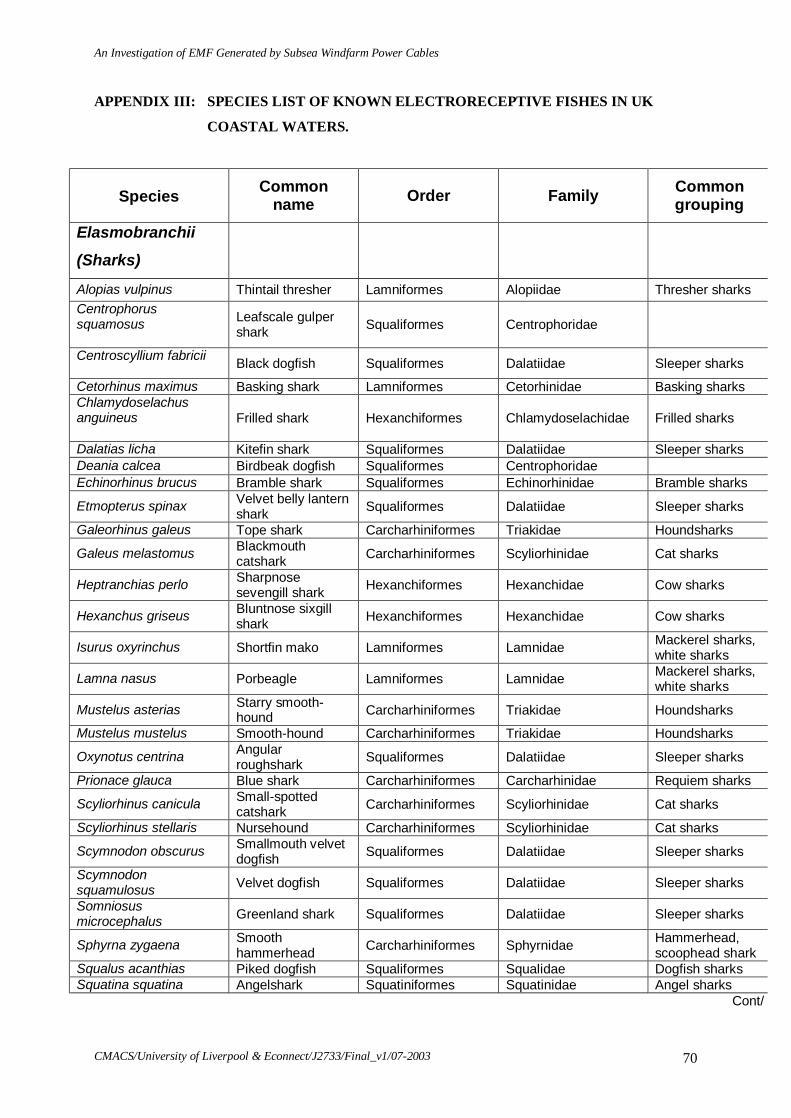
An Investigation of EMF Generated by Subsea Windfarm Power Cables
CMACS/University of Liverpool & Econnect/J2733/Final_v1/07-2003 70
APPENDIX III: SPECIES LIST OF KNOWN ELECTRORECEPTIVE FISHES IN UK
COASTAL WATERS.
Species
Common name Order Family Common
grouping Elasmobranchii (Sharks)
Alopias vulpinus Thintail thresher Lamniformes Alopiidae Thresher sharks Centrophorus squamosus
Leafscale gulper shark Squaliformes Centrophoridae
Centroscyllium fabricii Black dogfish Squaliformes Dalatiidae Sleeper sharks
Cetorhinus maximus Basking shark Lamniformes Cetorhinidae Basking sharks Chlamydoselachus anguineus
Frilled shark Hexanchiformes Chlamydoselachidae Frilled sharks
Dalatias licha Kitefin shark Squaliformes Dalatiidae Sleeper sharks Deania calcea Birdbeak dogfish Squaliformes Centrophoridae Echinorhinus brucus Bramble shark Squaliformes Echinorhinidae Bramble sharks
Etmopterus spinax Velvet belly lantern shark Squaliformes Dalatiidae Sleeper sharks
Galeorhinus galeus Tope shark Carcharhiniformes Triakidae Houndsharks
Galeus melastomus Blackmouth catshark Carcharhiniformes Scyliorhinidae Cat sharks
Heptranchias perlo Sharpnose sevengill shark Hexanchiformes Hexanchidae Cow sharks
Hexanchus griseus Bluntnose sixgill shark Hexanchiformes Hexanchidae Cow sharks
Isurus oxyrinchus Shortfin mako Lamniformes Lamnidae Mackerel sharks, white sharks
Lamna nasus Porbeagle Lamniformes Lamnidae Mackerel sharks, white sharks
Mustelus asterias Starry smooth-hound Carcharhiniformes Triakidae Houndsharks
Mustelus mustelus Smooth-hound Carcharhiniformes Triakidae Houndsharks
Oxynotus centrina Angular roughshark Squaliformes Dalatiidae Sleeper sharks
Prionace glauca Blue shark Carcharhiniformes Carcharhinidae Requiem sharks
Scyliorhinus canicula Small-spotted catshark Carcharhiniformes Scyliorhinidae Cat sharks
Scyliorhinus stellaris Nursehound Carcharhiniformes Scyliorhinidae Cat sharks
Scymnodon obscurus Smallmouth velvet dogfish Squaliformes Dalatiidae Sleeper sharks
Scymnodon squamulosus Velvet dogfish Squaliformes Dalatiidae Sleeper sharks
Somniosus microcephalus Greenland shark Squaliformes Dalatiidae Sleeper sharks
Sphyrna zygaena Smooth hammerhead Carcharhiniformes Sphyrnidae Hammerhead,
scoophead shark Squalus acanthias Piked dogfish Squaliformes Squalidae Dogfish sharks Squatina squatina Angelshark Squatiniformes Squatinidae Angel sharks Cont/

An Investigation of EMF Generated by Subsea Windfarm Power Cables
CMACS/University of Liverpool & Econnect/J2733/Final_v1/07-2003 71
Elasmobranchii (Skates & Rays)
Amblyraja hyperborea Arctic skate Rajiformes Rajidae Skates Amblyraja radiata Thorny skate Rajiformes Rajidae Skates Bathyraja spinicauda Spinetail ray Rajiformes Rajidae Skates Dasyatis pastinaca Common stingray Rajiformes Dasyatidae Stingrays
Dipturus batis Blue skate/common skate
Rajiformes Rajidae Skates
Dipturus oxyrinchus Longnosed skate Rajiformes Rajidae Skates Leucoraja circularis Sandy ray Rajiformes Rajidae Skates Leucoraja fullonica Shagreen ray Rajiformes Rajidae Skates Leucoraja naevus Cuckoo ray Rajiformes Rajidae Skates
Mobula mobular Devil fish Rajiformes Myliobatidae Eagle and manta rays
Myliobatis aquila Common eagle ray Rajiformes Myliobatidae Eagle and manta rays
Raja brachyura Blonde ray Rajiformes Rajidae Skates Raja clavata Thornback ray Rajiformes Rajidae Skates Raja microocellata Small-eyed ray Rajiformes Rajidae Skates Raja montagui Spotted ray Rajiformes Rajidae Skates Raja undulata Undulate ray Rajiformes Rajidae Skates Rajella fyllae Round ray Rajiformes Rajidae Skates Rostroraja alba Bottlenosed skate Rajiformes Rajidae Skates Torpedo marmorata Spotted torpedo Torpediniformes Torpedinidae Electric rays Torpedo nobiliana Atlantic torpedo Torpediniformes Torpedinidae Electric rays Holocephali (Chimaeras)
Chimaera monstrosa Rabbit fish Chimaeriformes Chimaeridae Shortnose chimaeras or ratfishes
Agnatha (Jawless fish)
Lampetra fluviatilis European river lamprey Petromyzontiformes Petromyzontidae Lampreys
Petromyzon marinus Sea lamprey Petromyzontiformes Petromyzontidae Lampreys
Note: All species shown have been recorded in UK coastal waters at depths less than 200m.
Data sources:
Froese, R. and D. Pauly. eds. (2003). FishBase. World Wide Web electronic publication.
www.fishbase.org, version 04 June 2003.
Vas, P. (1991). A field guide to the sharks of British coastal waters. Field Studies Council
AIDGAP Publication No. 205.