Final report on New Zealand sea lion pupping rate

Final report on New Zealand sea lion pupping rate

NIWA Client Report: WLG2008-77 November 2008 NIWA Project: DOC08302

Final report on New Zealand sea lion pupping rate Authors D.J. Gilbert B.L. Chilvers Prepared for

Department of Conservation Project

POP2006-01 Objective 3. Analysis from sea lion database to estimate pupping rate and associated parameters

NIWA Client Report: WLG2008 -77 November 2008 NIWA Project: DOC08302 National Institute of Water & Atmospheric Research Ltd 301 Evans Bay Parade, Greta Point, Wellington Private Bag 14901, Kilbirnie, Wellington, New Zealand Phone +64-4-386 0300, Fax +64-4-386 0574 www.niwa.co.nz

Contents 1. Introduction 1 2. Model 1 3. Data 2 4. Preliminary analyses 3 5. Estimable parameters 5 6. Pupping rate and survival 6 7. Likelihoods 6 8. Results 10 9. Discussion 11 References 15

Reviewed and Approved for release by:

Dr Don Robertson

Chief Scientist Biodiversity and Biosecurity

Executive summary We have used data from 11 cohorts of female New Zealand sea lions on the Enderby Island rookery, tagged between 1987 and 2003 and observed between 1999-2000 and 2006-07, to estimate pupping rate. In our previous criterion-based model it was assumed that all breeding animals are seen and positively identified as breeders during a season. However because most individuals’ breeding states cannot be categorically determined we developed a mixture model in which probabilities of breeding or not breeding are assigned and corresponding likelihoods are added. Pupping rate was estimated as a domed function of age determined by five parameters. The maximum rate was reduced by a factor of 0.33 if a cow had not bred in the previous season. The population mean reached its maximum of 0.49 y-1 at age 12 years. Without the model our preliminary pupping rate calculation under-estimated breeders because not all of them produce breeder observations but also under-estimated live animals because some animals survive beyond their last sighting. The model estimate shows that the preliminary calculations tend to slightly over-estimate pupping rate. First year survival varied considerably amongst cohorts. That for the 1998 cohort, which was affected by an epizootic, was estimated to be only 0.24 y-1, implying that considerable mortality occurred after the first two months, for which Chilvers et al. (2007) estimated survival of 0.58 y-1. The breeding rate of this cohort was also shown to be considerably lower than the estimated population mean. Our pupping rate estimate suggests that sea lions may be less productive than previously thought and implies a lower maximum population growth rate. If our pupping rate estimate is used in a population model it should be done so that other parameters, especially population size, are estimated consistently with it. This is the final report for this project.

Final report on New Zealand sea lion pupping rate iv

1. Introduction Our initial report under Department of Conservation, Project POP2006-01, Objective 3 (Gilbert 2007) discussed the viability of estimating pupping rate for New Zealand sea lions from the tag-resighting data collected during the summer breeding season on Enderby Island between 1999–2000 and 2006–07. Hereafter we refer to these seasons as 2000 and 2007, etc. Our second report described a mixture model in which observations were made up of mixtures of breeders and non-breeders, high and low fecundity cows, and high and low visibility cows. We use the term breeder to refer to a cow that has a pup in a particular season, including a stillbirth or pup that dies. This mixture model failed to satisfactorily fit the data. A criterion-based model in which it is assumed that all breeding animals are seen and are positively identified as breeders during a season was then developed for our third report. Estimation by maximum likelihood involves simpler formulae than for the mixture model and gave plausible estimates of pupping rate and mortality (including tag loss). In this final report we describe another mixture model. Preliminary analyses showed that when a breeder is observed, breeder observations, i.e. observations that identify a breeder, are only made with probability of about 0.35. Therefore some breeders will be seen but not identified as such. These analyses also showed that the probability of breeding depends strongly on whether a cow has bred in the previous season. We therefore developed another mixture model in which every possible scenario of breeder/non-breeder state between 2000 and 2007 was included with an associated probability dependent on age, and the likelihood of the set of observations for each animal was calculated. This model estimated the pupping rate function and other parameters without identifying animals each season as breeders or non-breeders.

2. Model To estimate pupping rate, we have developed a statistical model to explain the annual behavioural observation frequencies of the tagged sea lion cows. It is governed by a set of parameters, which are estimated by maximum likelihood. It is desirable to reduce the number of estimable parameters by expressing relationships as algebraic functions. Over-parameterisation leads to estimates that lack robustness and tend to reflect random variations in the data rather than underlying relationships. The preliminary estimate of pupping rate in Gilbert (2007) has implausible spikes at ages 9, 12, 16 and 19 years. Here we express both mortality and pupping rate as domed functions of age, parameterised so that the parameters are meaningful. For example, β1 is a maximum pupping rate and that occurs for cows aged between ages β2 and β2 + β5 years. The model developed by Gilbert & Chilvers (2008) used a criterion based on the observations to determine whether a cow had pupped in a given season. The experience of the field teams is that because of the necessity of a cow to return regularly to her pup, she will almost always be observed. Non-breeders are not necessarily seen and the proportion observed must be estimated. The problem with the criterion-based approach is that not all observations of breeders are breeder observations, i.e. observations that identify a breeder. If there is a probability less than one that when a breeder is seen a breeder observation will be made, then there is a finite probability that a breeder will not be identified as such. The criterion-based approach will under-estimate breeders.

Final report on New Zealand sea lion pupping rate 1

We have therefore developed a mixture model in which an individual’s behavioural observations are modelled as a probabilistic mixture of breeder and non-breeder observations. Only individuals that produce a birth or dead pup observation are categorically identified as breeders. Only juveniles are categorically identified as non-breeders. The mixture model calculates the probability that an individual will breed in a season and multiplies this by the probability that the actual observations would be made if it did. Likewise it calculates the probability that an individual will not breed and multiplies this by the probability that the observations would be made if it did not. These products are added. The calculation is complicated by the fact that breeding appears to be serially correlated (Gilbert 2008). A cow that has bred in one season is more likely to breed in the next than a cow that has not. Therefore the model uses scenarios of breeder/non-breeder sequences between 2000 and 2007. For each cow the probability of each scenario depends on the age of the cow via the pupping rate function, and on the serial correlation parameter, which modifies the pupping rate according to whether a season follows previous breeding or non-breeding. Each scenario therefore has a probability and a likelihood that it would produce the actual sequence of observations. Some probabilities are zero; for example when the scenario includes an immature cow breeding. The products of the scenario probabilities and the likelihoods are added.

3. Data 2274 female pups were tagged during summer field trips in 1987, 1990–93 and 1998–2003 and 1345 of these were observed in the 2000 – 2007 seasons (Table 1). Because adequate behavioural observations commenced in 2000, the only data used prior to that season are the seasons of tagging. Most of the 1987 and 1990 cohorts had died, lost their tags or ceased breeding by 2000. Observations of the 2000–2003 cohorts include the tagging event. During 2000 some animals were branded. Cows were observed intensively until it could be established that they had pupped and these were branded. Some of these already had tags. Those that did not were of unknown age and were therefore not included in this analysis. Some pups were also branded and are included. The data are stored in a master spreadsheet. They were read into the R package for checking and preliminary analysis. Consistency checks were made on variables for “season” (e.g. December 2005 – February 2006 is defined as the 2006 season), “age” and “tag season” and a small number of errors and omissions were corrected. Unique tag identifiers were generated. The numerical tag numbers are not unique because in a few cases the same numbers had been used with different tag types and colours. Unique identifiers were generated by concatenating “colour”, “shape” and “tag number”. The unique tag identifier associated with the first tag applied to an animal was assigned to all records of that animal. The key information required to estimate pupping rate is the observed behaviour, which is contained in a free format “behaviour comments” field. To allow analysis each comment was converted to a code corresponding to one of the following: “pregnant”, “giving birth”, “with stillbirth”, “with dead pup”, “nursing pup”, “nursing yearling”, “with pup”, “calling”, “nothing relevant”, “suckling from cow” and “dead”. The conversion of each comment to a code was achieved by searching for key words in the “behaviour comments” field and examining each distinct comment. Determining the correct codes was straightforward if somewhat time-consuming. Examination of the data in this form indicated that a further reduction to just three behaviour categories would facilitate estimation of pupping rate. The “pregnant”


behaviour was not a direct observation but rather an interpretation based on subsequent observations. It was therefore treated as equivalent to “nothing relevant”. The three categories used were: “total”, “breeder observation” and “birth observation”. The “birth observation” behaviour grouping refers to the behaviours: “giving birth”, “with stillbirth”, “with dead pup” and “branding”. This last category was derived from another field in the spreadsheet and was based on the fact that the only cows branded in 2000 were those that had been positively identified as breeders. Obviously the branding of a pup was not coded as a “birth observation”. The “breeder observation” behaviour grouping refers to: “nursing pup”, “with pup” or “calling”. These three behaviours almost always indicate breeding but are occasionally recorded for non-breeders. We now describe the data. Let n¸ a, i, and y denote tag identifier, age, behaviour category and season. The data was arranged in the following format:

1. The number of tagged cows, N 2. An N × 4 matrix, each row containing: tag identifier n, tag season yT, the last

resight season yL, and whether the cow was branded in 2000, B (value 1 if branded and 0 otherwise). In season y the age of a particular cow would be

. yTy y− L is required because in the seasons following yL the possibilities of both death and survival without sighting must be included in the likelihood formulae. For cows where there have been no observations during 2000 – 2007, yL is null.

3. An array of N matrices, each with three rows and 8 columns. There is one

matrix for each tagged cow and a column for each of the seasons, 2000 – 2007. The rows contain the frequency of each behaviour grouping: “total”, “breeder observation” and “birth observation”. If at least one “birth observation” is observed, the row will contain a one and otherwise a zero. The other groupings contain counts of observations. For a given tag identifier in season y, the data in the corresponding row of the array is denoted by yx

%=

(xy0, xy1, xy2).

4. Preliminary analyses It is likely that the criterion-based approach developed Gilbert & Chilvers (2008) under-estimated breeders. Figure 1 shows the distribution of observation frequencies for cows with birth observations and the contrasting frequencies for juveniles, too young to breed. Although the majority of known breeders have at least one breeder observations, some have none. The probability that an observation of a breeder will record a “breeder observation” is about one third (Figure 1: sloping line). Therefore there is a finite probability that we will have no breeder observation of a particular breeding cow, especially if it is one that is seen only a few times in the season. Figure 1 does show some definite breeders for which no breeder observation was made. Some of these are where a stillbirth has occurred. The distribution of total observations for branded definite breeders suggests that the proportion with zero total observations is negligible, but for tagged, definite breeders a small proportion of zeros is indicated by the existence of some low counts. The difference is caused by the more easily discerned branded cows compared to those with tags alone. The distributions of juveniles and apparent non-breeders in Figure 1 have modes near 1, which suggests that a considerable proportion of non-breeders are not observed at all. A model to estimate pupping rate must therefore


estimate and account for the proportion of both breeders and non-breeders that are alive but not observed and of breeders that are observed but for which no breeder observation is made. The histograms of total observation frequencies suggest overdispersion for both breeders and non-breeders (Figure 2). This means that the Poisson distribution, commonly used to model this kind of data would not adequately capture its variability. Instead the negative binomial distribution was used to model total observations. Branded cows are seen about twice as often as those with tags alone. The brands are large and being on the animals’ torsos, are less likely to be hidden than the tags, which are attached to the flippers. A parameter that scaled up the mean frequency of tagged animals to give that of branded animals was applied. Cows that have at least one breeder observation display very similar frequency distributions to definite breeders. They are therefore probably almost all breeders. Field workers occasionally make breeder observations of non-breeders. We therefore include a parameter for the probability of this, but these plots suggest that its value will be small. If a breeder has no breeder observation it cannot be identified as such and is therefore not included in these histograms of probable breeders. Such animals would on average have lower total observation frequencies than those plotted. The frequency histograms of 3-year-olds have substantially smaller means than the probable breeders and their shape suggests many are not seen at all (many zeros). Histograms of total observations for cows with no breeder observations (not shown) are similar to those of 3-year-olds. We therefore model the non-breeders and the juveniles with negative binomial distributions, but the parameters for the means will take substantially smaller values than those for breeders. We calculated preliminary estimates of the pupping rate function based on the ratio of breeders to total cows known to be alive by age. For this purpose we identify breeders as those that had at least one breeder observation in a season (Figure 3). The population mean line has a plausible domed shape with maximum values between 9 and 13 years. There are two problems with this approach. The first is that breeders that did not have breeder observations will be counted as non-breeders and the second is that some live animals (mostly non-breeders) are not seen and will not be included in the denominator of the ratio. The difference in pupping rate between those cows that pupped the previous season and those that did not is considerable (Figure 3). Amongst the latter there is also a considerable difference between those that were seen and those that were not (but were seen in a subsequent season). This second difference suggests that some cows either do not return to the rookery at all or do so fleetingly. A cow that spends little or no time on the rookery is obviously unlikely to copulate. Our model contains a parameter that expresses the pupping rate of previous non-breeders as a fraction of that of breeders but does not separate non-breeders into those that do and do not return to the rookery. Preliminary estimates of survival rate show a low survival of pups, a high maximum survival at 2 years and a gradual decline thereafter (Figure 4). The estimate for each cohort is the ratio of cows known to be alive in one season to those in the previous season. There are two problems with this approach. The first is that this definition of survival necessarily includes the retention and readability of at least one tag or brand. Tag loss may vary between individuals because different tags were used, some animals received only one tag, some animals were branded and some had microchip transponders implanted. The survival estimated here therefore under-estimates true survival. The second problem is that some live animals are not seen each season. This omission of animals will bias the ratios downwards and will have the greatest effect in


the final season (2007). The most recent survival for each cohort (2006 to 2007) will be the most negatively biased. This partly explains the apparent step at age 7 years between the early 1990s cohorts and the more recent ones. The preliminary estimates indicate that an asymmetrically domed function should be used to model survival.

5. Estimable parameters The estimable parameters are given here. We define pupping rate as a domed function of age with a plateau, which gives the

probability that a cow will bear a pup in a given season. The function is determined by a vector of parameters, β

%, where β1 is the maximum value of the

function, the plateau over which the maximum occurs lies between ages β2 and β2 + β5 years, and β3 and β4 are the ages at which the left and right-hand limbs of the function fall to half the maximum. All the elements of β

% may take non-

integer values, let α be the factor by which the pupping rate function is reduced if a cow did not breed

in the previous season, 0 < α < 1, we obtain survival via mortality, which is defined as a U-shaped function of age

determined by a vector of parameters, μ%

that gives the probability that a cow will die or lose its second tag in the season after achieving a given age, where μ1 is the minimum function value (mortality rate), μ2 is the age in years at which the minimum is achieved, μ3 is the function value at age 0 years, μ4 is the function value at age 20 years, and μ5 determines the curvature of the function,

let be a vector that determines the mortality (and tag loss) of each tagged cohort in its first season. Hence, for example, 1 – M

Μ%

1987 is the proportion of the tagged female pups that survive to age 1 year,

let θ03, θ20 and θ2 be the mean frequency of total observations of a 3-year-old (non-breeder), of a 20-year-old non-breeder, and of a 1- or 2-year-old in a season under the negative binomial distribution, θ03, θ20 and θ2 > 0. Non-breeders between 3 and 20 years old have total observation frequencies linearly interpolated between θ03 and θ20,

let θ1 be the mean frequency of total observations of a breeder in a season, θ1 > 0, let φ be the factor that multiplies the mean frequency of observations for branded cows

(does not apply to season 2000 because brands were applied late January). The probability of positively identifying a breeder is increased by the same factor, φ > 1,

let χ be the factor by which the frequency of zeros (not observed) for a non-breeder (including 1- to 3-year-old cows) is reduced ,

let ρ%

be a vector of multipliers that scale the mean frequencies of total observations,

the θ’s, for the seasons, 2000-2007. These multipliers apply to breeders and non-breeders. ρ2007 is fixed at 1 to avoid over-parameterisation,

let γ0 and γ1 be the variance to mean ratio of total observation frequencies of non-breeders and of breeders,

let π0 and π1 be the mean proportion of breeder observations for a given total frequency of observations for a non-breeder (sic) and a breeder, 0 < π0 < 1 and 0 < π1 < 1,

let κ be the parameter that determines the variance of breeder observation frequencies for a given total number of observations in a season under the beta-binomial distribution (as κ tends to ∞ the beta-binomial tends to the binomial, κ > 0 ,

let ϕ%

be a vector of season probabilities of making a birth observation.


6. Pupping rate and survival The pupping rate function expresses the probability that a cow of a given age will bear a pup in a given season, and therefore implicitly includes maturation of cows. We therefore expect it to have a rising left hand limb, to reach a maximum between 8 and 14 years and then to decline gradually with age. This is the empirical shape found by Chilvers (2006) and Gilbert (2007). The probability of breeding depends on whether a cow has bred in the previous season. The function we define depends on parameter vector β

% and gives the mean rate for cows that have bred in the previous season,

22

3 2

22 5

4 2 5

1 2

1 2 2

1 2

0 3

2 b( | )

2

a

a

a

aa

a

a

ββ β

β ββ β β

5

5

β ββ

β β β β

β β β

⎛ ⎞−−⎜ ⎟

−⎝ ⎠

⎛ ⎞− −−⎜ ⎟

− −⎝ ⎠

≤⎧⎪⎪⎪ ≤⎪= ⎨ < ≤ +⎪⎪⎪

> +⎪⎩

%

The function has a maximum value of β1 for a between β2 and β2 + β5 and takes the value 0.5β1 at a = β3 on the left of the maximum and at a = β4 on the right. The pupping rate for cows that have not bred in the previous season is reduced to

b( | )aα β×%

. The mean pupping rate for the population is given iteratively by,

b( | ) if 4b ( | )

b( | ) (1 )b ( 1| ) if 4

a aa

a a

α ββ

β α α β

=⎧⎪′ = ⎨ ⎡ ⎤′ a+ − − >⎪ ⎣ ⎦⎩%

%

% %We require a survival rate for each age class to determine how many cows were still alive in each season. We define this by defining mortality at age a as the probability that a cow of age a on 1 January dies between the preceding 1 December and the following 30 November. Survival is expected to be an asymmetrically domed function, typical of vertebrates, with low survival for the youngest animals, increasing steeply to a maximum and then declining gradually (Begon et al. 2006, Goodman 1981). Mortality includes incidental bycatches in fisheries (largely squid trawling) but also second tag loss and loss of tag readability. Tag loss could be estimated more satisfactorily separately by using the numbers of animals that have retained one and two tags but tag loss was outside the scope of this project and its precise estimation was not essential to estimating pupping rate. The mortality function depends on parameter vector μ

%,

522

522

03

1 21

204

1 21

m( | )

a

a

aa

a

μ

μ

μμ

μμ

μμ μ

μμ

μμ μμ

⎛ ⎞−⎜ ⎟−⎝ ⎠

⎛ ⎞−⎜ ⎟

−⎝ ⎠

⎧⎪ ⎛ ⎞

≤⎪ ⎜ ⎟⎪ ⎝ ⎠= ⎨⎪

⎛ ⎞⎪ >⎜ ⎟⎪⎝ ⎠⎩

%

The function has a minimum value of μ1 at age a = μ2, takes the value μ3 at a = 0 and μ4 at a = 20. Estimating μ

% therefore gives the mean mortality plus tag loss rates for

the population. We present estimates as survival rates, i.e. 1 m( | )a μ−%

.

7. Likelihoods The method of maximum likelihood obtains parameter estimates by finding the set of values that make the whole set of observations the most likely. To achieve this, the likelihood must be expressed as an algebraic function of the parameters. It is built up by multiplying together the probabilities of the independent subsets of observations.


The time series of observations of each cow makes up each subset. There is dependence between successive seasons because breeding is less likely for a cow that did not breed the previous season and because the likelihood of mortality in a season is zero if any subsequent observations were made. The mixture model described by Gilbert (2008) failed to produce meaningful estimates. Gilbert & Chilvers (2008) used a criterion-based model where it was assumed that the observations showed categorically all cows that had pupped in a given season. More careful examination of the data suggested that a small proportion of breeders would, by chance, produce no breeder observation. The frequency of total observations in a season was clearly a function of whether the cow had pupped or not (Figures 1 and 2). By examining the frequencies of total observations (xy0’s) of those cows that had birth observations and 3-year-olds that cannot have pupped it was possible to infer that the mean frequency of total observations of breeders was about 13 and of non-breeders about 3 (where zeros are included in the distribution). It could also be ascertained that branded cows were about twice as likely to be observed as those that were merely tagged. These frequency distributions were over-dispersed relative to the Poisson distribution. Total observation frequencies were assumed to be distributed negative binomially. For a given frequency of total observations in a season the proportion of breeder observations appeared to be constant (about 0.35, Figure 1). The frequencies of breeder observations were over-dispersed relative to the binomial distribution. They were assumed to be distributed beta-binomially, conditional on total observations. Because we no longer assume that we can categorically identify breeders and non-breeders and the observations of each cow are not independent, it is necessary to calculate the likelihood for each possible breeding scenario and add them. Let Zys be an element of the matrix that denotes whether a cow has bred in season y under scenario s, where 1 denotes breeding and 0 non-breeding. There are 256 possible sequences of 1’s and 0’s. We use .sZ

% to denote the time series for scenario s.

For a particular cow we can obtain an expression for the probability of a particular scenario. In what follows we omit the parameters from the pupping rate and mortality functions for clarity. The probability of the breeding state specified by Z.s in season 2000 can be conveniently specified by,

[ ] ( )( )2000 T 2000 T 2000P b (2000 ) 1 b (2000 ) 1s s sZ y Z y′ ′= − + − − − Z Because we have no data to indicate breeding prior to 2000 the unconditional pupping rate function, b ()′ , must be used (actually a very few observations were made in 1998 and 1999 but have not been used). After 2000 we must account for both the current and the previous breeding state specified by the scenario and use the conditional pupping rate function,

[ ]( )( ){ }

( )( )( ) ( )( )( )

.

T 2000 T 2000

2007 T 1 T 1

2001 T 1 T

P

b (2000 ) 1 b (2000 ) 1

b( ) 1 b( ) 1

b( ) 1 1 b( ) 1 1

s

s s

ys y s ys y s

y ys y s ys y s

Z

y Z y Z

y y Z Z y y Z Z

y y Z Z y y Z Zα α

− −

= − −

=

′ ′− + − − −

⎡ ⎤− + − − −⎢ ⎥×⎢ ⎥+ − − + − − − −⎣ ⎦

∏

%

1

If age, then exactly one term inside the square brackets is non-zero. If then

T 3y y− >

T 3y y− ≤ Tb( )y y− = 0 , so if Zys = 1 the scenario is impossible and its probability is zero.


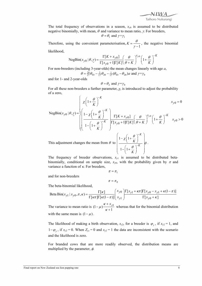
The total frequency of observations in a season, xy0 is assumed to be distributed negative binomially, with mean, θ and variance to mean ratio, γ. For breeders,

1 1and =θ θ γ γ=

Therefore, using the convenient parameterisation,1

K θγ

=−

, the negative binomial

likelihood, 00

00

[ ]NegBin( | , ) 1

[ 1] [ ]

yx Ky

yy

K xx

x K K Kθ θθ γ

θ

−Γ + ⎛ ⎞ ⎛ ⎞= +⎜ ⎟ ⎜ ⎟Γ + Γ +⎝ ⎠ ⎝ ⎠%

For non-breeders (including 3-year-olds) the mean changes linearly with age a, 20 3 1

03 20 03 20 017 17 17 ( ) and a =θ θ θ θ θ γ= − − − γ and for 1- and 2-year-olds

2 0and =θ θ γ γ= For all these non-breeders a further parameter, χ, is introduced to adjust the probability of a zero,

0

0

00

0

1 0

NegBin( | , ) 1 1 [ ]1

[ 1] [ ]1 1

y

K

y

Ky x K

yK y

xK

xK xK x

x K K K

K

θχ

θθ γ χθ θ

θθ

−

−

−

−

⎛ ⎞+ =⎜ ⎟⎝ ⎠

⎛ ⎞⎛ ⎞= ⎜ ⎟− +⎜ ⎟ Γ + ⎛ ⎞ ⎛ ⎞⎜ ⎝ ⎠ ⎟ +⎜ ⎟ ⎜ ⎟⎜ ⎟ Γ + Γ +⎝ ⎠ ⎝ ⎠⎛ ⎞⎜ ⎟− +⎜ ⎟⎜ ⎟⎝ ⎠⎝ ⎠

%0 0y

⎧⎪⎪⎪⎪⎨⎪ >⎪⎪⎪⎩

This adjustment changes the mean from θ to 1 1

1 1

K

KK

K

θχθ

θ

−

−

⎛ ⎞⎛ ⎞⎜ ⎟− +⎜ ⎟⎜ ⎝ ⎠ ⎟⎜ ⎟

⎛ ⎞⎜ ⎟− +⎜ ⎟⎜ ⎟⎝ ⎠⎝ ⎠

.

The frequency of breeder observations, xy1 is assumed to be distributed beta-binomially, conditional on sample size, xy0, with the probability given by π and variance a function of κ. For breeders,

1π π= and for non-breeders

0π π= The beta-binomial likelihood,

0 1 0 11 0

1 0

[ ] [ (1[ ]Beta Bin( | , , )[ ] [ (1 )] [ ]

y y y yy y

y y

x x x xx x

x x)]κπ κκπ κ

κπ κ π κ

⎛ ⎞ Γ + Γ − + −Γ= ⎜ ⎟⎜ ⎟Γ Γ − Γ +⎝ ⎠

π

The variance to mean ratio is 0(1 )1yxκ

μκ+

−+

whereas that for the binomial distribution

with the same mean is (1 )μ− . The likelihood of making a birth observation, xy2, for a breeder is yϕ , if xy2 = 1, and 1 yϕ− , if xy2 = 0. When Zys = 0 and xy2 = 1 the data are inconsistent with the scenario and the likelihood is zero. For branded cows that are more readily observed, the distribution means are multiplied by the parameter, φ.


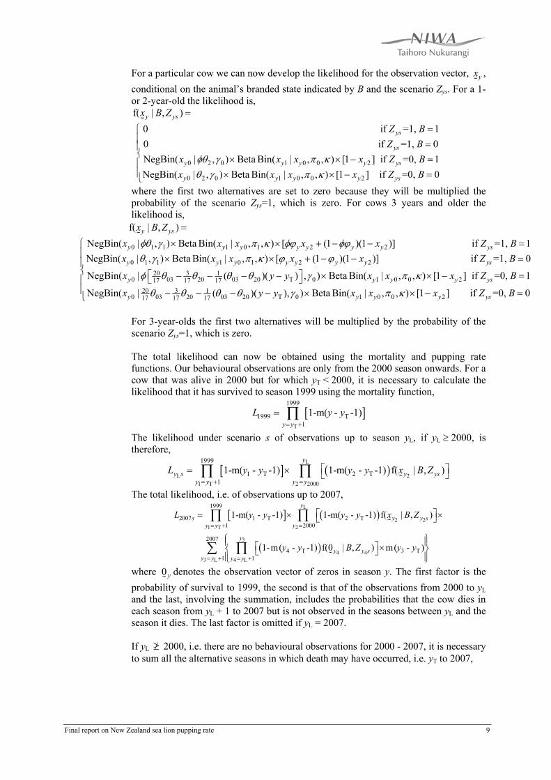
For a particular cow we can now develop the likelihood for the observation vector, yx%

, conditional on the animal’s branded state indicated by B and the scenario Zys. For a 1- or 2-year-old the likelihood is, f( | , )

0 y ysx B Z =%

0 2 0 1 0 0 2

0 2 0

if =1, 10 if =1, 0NegBin( | , ) Beta Bin( | , , ) [1 ] if =0, 1NegBin( | , )

ys

ys

y y y y ys

y

Z BZ B

x x x x Zx

φθ γ π κθ γ

==

B× × − =

1 0 0 2Beta Bin( | , , ) [1 ] if =0, 0y y y ysx x x Z Bπ κ

⎧⎪⎪⎨⎪⎪ × × −⎩ =

where the first two alternatives are set to zero because they will be multiplied the probability of the scenario Zys=1, which is zero. For cows 3 years and older the likelihood is,

0 1 1 1 0 1 2 2

f( | , ) NegBin( | , ) Beta Bin( | , , ) [ (1 )(1 )]

y ys

y y y y y y y

x B Zx x x x xφθ γ π κ φϕ φϕ

=

× × + − −%

0 1 1 1 0 1 2 220 3 1

0 03 20 03 20 T 017 17 17

if =1, 1NegBin( | , ) Beta Bin( | , , ) [ (1 )(1 )] if =1, 0

NegBin( | ( )( ) , ) B

ys

y y y y y y y ys

y

Z Bx x x x x Z

x y y

θ γ π κ ϕ ϕ

φ θ θ θ θ γ

B=

× × + − −

⎡ ⎤− − − − ×⎣ ⎦

=

1 0 0 2

20 3 10 03 20 03 20 T 0 1 0 0 217 17 17

eta Bin( | , , ) [1 ] if =0, 1

NegBin( | ( )( ), ) Beta Bin( | , , ) [1 ] if =0, 0y y y ys

y y y y ys

x x x Z B

x y y x x x

π κ

θ θ θ θ γ π κ

⎧⎪⎪⎨ × − =⎪⎪ Z B− − − − × × − =⎩

For 3-year-olds the first two alternatives will be multiplied by the probability of the scenario Zys=1, which is zero. The total likelihood can now be obtained using the mortality and pupping rate functions. Our behavioural observations are only from the 2000 season onwards. For a cow that was alive in 2000 but for which yT < 2000, it is necessary to calculate the likelihood that it has survived to season 1999 using the mortality function,

[ ]T

1999

1999 T1

1-m( - -1)y y

L y= +

= ∏ y

B Z

The likelihood under scenario s of observations up to season yL, if yL ≥ 2000, is therefore,

[ ] ( )L

L 21 T 2 2000

1999

1 T 2 T1

1-m( - -1) 1-m( - -1) f( | , )y

y s y ysy y y y

L y y y y x= + =

⎡ ⎤= × ⎣ ⎦∏ ∏%

The total likelihood, i.e. of observations up to 2007,

[ ] ( )

( )

L

2 21 T 2

3

4 43 L 4 L

1999

2007 1 T 2 T1 2000

2007

4 T 3 T1 1

1-m( - -1) 1-m( - -1) f( | , )

1-m( - -1) f(0 | , ) m( - )

y

s y y sy y y

y

y y sy y y y

L y y y y x B

y y B Z y y

= + =

= + = +

Z⎡ ⎤= × ×⎣ ⎦

⎧ ⎫⎪ ⎪⎡ ⎤ ×⎨ ⎬⎣ ⎦⎪ ⎪⎩ ⎭

∏ ∏

∑ ∏

%

%

where %

denotes the observation vector of zeros in season y. The first factor is the probability of survival to 1999, the second is that of the observations from 2000 to y

0 y

L and the last, involving the summation, includes the probabilities that the cow dies in each season from yL + 1 to 2007 but is not observed in the seasons between yL and the season it dies. The last factor is omitted if yL = 2007. If yL 2000, i.e. there are no behavioural observations for 2000 - 2007, it is necessary to sum all the alternative seasons in which death may have occurred, i.e. y

≥/T to 2007,


( )

1

T1 T2

T2

3

4 43 4

1999

T T2007 2 11 1

1999

T21

2007

T T4 32000 2000

m(0)+ 1-m( - -1) m( - ) +

1-m( - -1)

1-m( - -1) f(0 | , ) m( - )

y

sy y y y

y y

y

y y sy y

L y y y

y y

y y B Z y y

= + = +

= +

= =

⎧ ⎫⎪ ⎪⎡ ⎤⎨ ⎬⎣ ⎦⎪ ⎪⎩ ⎭

⎡ ⎤⎣ ⎦

⎧ ⎫⎪ ⎪⎡ ⎤⎨ ⎬⎣ ⎦⎪ ⎪⎩ ⎭

= ×

×

×

∑ ∏

∏

∑ ∏%

y

If yT ≥ 2000 and yL ≥ 2000,

( )

( )

L

1 11 T

2

3 32 L 3 L

2007 1 T1

2007

3 T 2 T1 1

1-m( - -1) f( | , )

1-m( - -1) f(0 | , ) m( - )

y

s y y sy y

y

y y sy y y y

L y y x B Z

y y B Z y y

= +

= + = +

⎡ ⎤= ×⎣ ⎦

⎧ ⎫⎪ ⎪⎡ ⎤ ×⎨ ⎬⎣ ⎦⎪ ⎪⎩ ⎭

∏

∑ ∏

%

%

Where observations of the pup, which provides no relevant information, are not included. The expression for L2007s when yT 2000 is obtained similarly. ≥/ To obtain the unconditional likelihood of the observations it is necessary to obtain the sum of the scenario likelihoods weighted by the scenario probabilities,

[ ]2007. . 2007P s ss y

L Z L⎡ ⎤

= ⎢ ⎥⎢ ⎥⎣ ⎦

∑ ∏%

Estimation involves summing the negative logarithms of these likelihoods over the tags denoted by the pre-subscript, n,

( )2007.1ln

N

nn

L=

Λ = −∑

and minimising Λ with respect to the estimable parameters. Estimation was carried out by coding the above functions using AD Model Builder© (Otter Research Ltd, Nanaimo, Canada). This software minimises Λ by analytically calculating its derivatives with respect to the estimable parameters at each trial set of values and then using these derivatives to step in the direction in parameter space that reduces Λ. Starting values for the parameters were based on Gilbert & Chilvers (2008) and the preliminary analysis. Because of problems with the minimisation we were only able to find an approximate confidence interval for β1, the maximum pupping rate, based on Chi-squared type I error in its likelihood profile.

8. Results Minimisation of the negative log-likelihood, Λ, presented considerable problems. Λ contains 256 scenarios for each of 2274 tagged cows, each scenario involving the calculation of multiple terms. While some scenarios for some cows are automatically set to zero because they are inconsistent with the data, the total number of calculations is large. While we are confident that AD Model Builder calculated Λ correctly, it was apparent that it did not calculate its derivatives correctly. Changing the order of the tags gave the same value for Λ but a different value for the derivatives. It appears that there was insufficient available memory to store all the intermediate derivative calculations. Therefore we had to search for the minimum using a partial trial and error process. We supplied a range of starting values for the parameters and examined patterns in the residuals to find improvement in the likelihood. We therefore cannot be certain that our final values are exact maximum likelihood estimates, but they appear to be close. Calculating the likelihood was also too slow to allow the estimation of a


Bayesian posterior distribution and credibility intervals for the parameters. For these reasons our only estimate of precision was an approximate confidence interval for β1. The parameter estimates (Tables 2 and 3) are plausible and give satisfactory diagnostics. The nature of a mixture model means that diagnostics based on individuals would not be informative. Instead we obtained diagnostics by aggregating the observations and predictions for cohorts and for observation seasons. For each animal the parameters give an estimated probability density function for the frequency of total observation counts and of breeder observation counts. These are summed density functions, weighted by the probabilities that the animal is alive and a breeder or a non-breeder each season. They were plotted against the aggregated observations. These fit the data satisfactorily (Figures 5 - 8). The model tends to slightly under-estimate the frequency of single observations. The numbers known to be alive (from the data) are necessarily under-estimates and are typically less than the fitted numbers alive, especially for the 2007 season Our estimate of mean pupping rate has a maximum of 0.52 y–1 at age 11 years and lies above half this maximum between ages 6 and 16 years (Figure 9). This is a population mean for all cows and is obtained iteratively. A cow that bred in the previous season has a maximum breeding probability, β1 = 0.78 y–1 at ages 9 and 10 years whereas that of a previous non-breeder is just 0.26 y–1. The 95% confidence intervals for β1 given in Table 2 translate to the range (0.50, 0.54) for the population mean. The estimated survival rate function (Figure 4) has a maximum at age 2 years (96.6%). As discussed above, estimated survival includes tag retention and therefore under-estimates true survival. Early model fits showed systematic under- and over-estimation of individual cohorts across seasons and systematic under- and over-estimation of seasonal observations across cohorts. The simplest explanation for the first problem was that there was a variation in first year survival (including tag loss) amongst cohorts. Thus, 11 first-year mortality parameters, vector Μ

%, were added to the model and these reduced the

negative log-likelihood by 15.1 and therefore significantly improved the fit. Survival estimates were plausible and ranged from 0.20 (1987 cohort) to 0.82 (2003 cohort). To explain under-estimation of total observations in some seasons and over-estimation in others we hypothesised that there was a variation in observational intensity amongst seasons. Thus, 7 seasonal mean frequency scalars, vector ρ

%, were added to the model

and these reduced the negative log-likelihood by 154.2 and therefore significantly improved the fit. Estimates ranged from 0.50 (2000) to 1.16 (2003). This range is quite plausible. There were differences in the size of field teams, the lengths of trips and in the ancillary tasks that were carried out amongst seasons. Again, the pupping rate function is affected very little by whether or not ρ

% is included in the model.

Seven similar parameters were added to the model to explain the variability in the number of birth observations amongst seasons.

9. Discussion Our data contains tagged and branded females from Enderby Island; the cohorts 1987, 1990–1993, 1998, 1999, 2000–2003; and observation for the seasons 2000–2007. A model was used to estimate a pupping rate function that assigned probabilities of breeding and of dying each season as a function of age. Estimation was by way of a


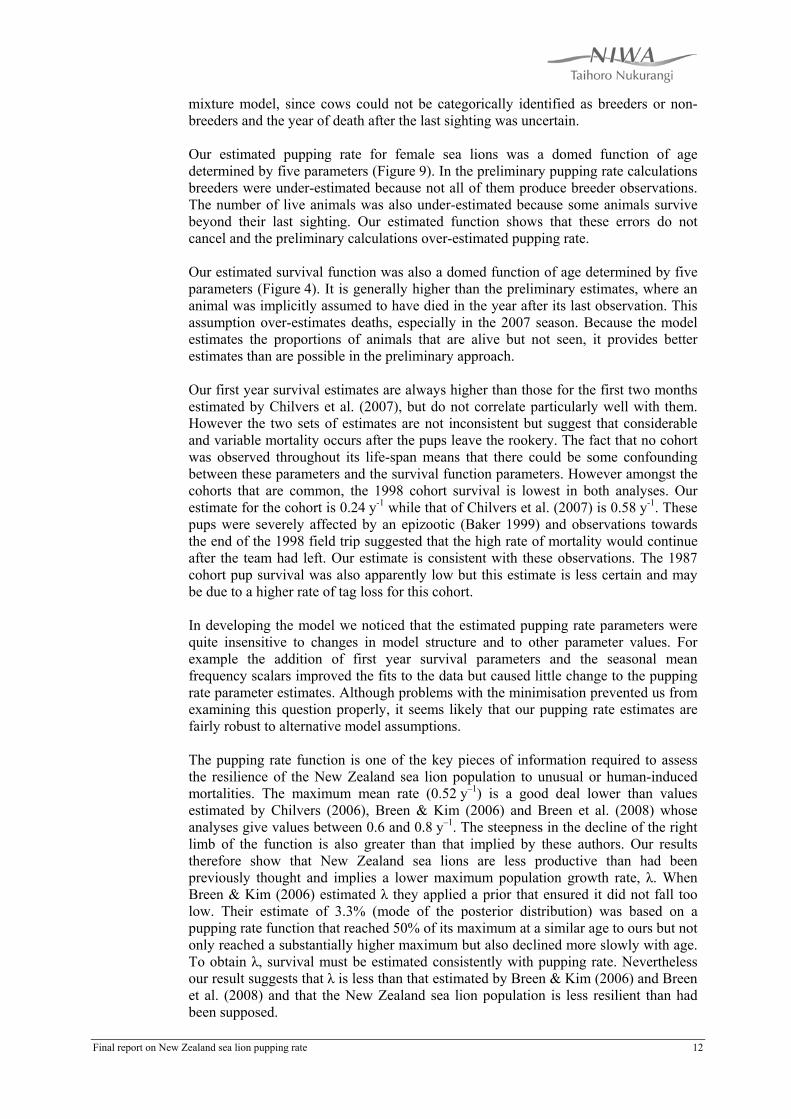
mixture model, since cows could not be categorically identified as breeders or non-breeders and the year of death after the last sighting was uncertain. Our estimated pupping rate for female sea lions was a domed function of age determined by five parameters (Figure 9). In the preliminary pupping rate calculations breeders were under-estimated because not all of them produce breeder observations. The number of live animals was also under-estimated because some animals survive beyond their last sighting. Our estimated function shows that these errors do not cancel and the preliminary calculations over-estimated pupping rate. Our estimated survival function was also a domed function of age determined by five parameters (Figure 4). It is generally higher than the preliminary estimates, where an animal was implicitly assumed to have died in the year after its last observation. This assumption over-estimates deaths, especially in the 2007 season. Because the model estimates the proportions of animals that are alive but not seen, it provides better estimates than are possible in the preliminary approach. Our first year survival estimates are always higher than those for the first two months estimated by Chilvers et al. (2007), but do not correlate particularly well with them. However the two sets of estimates are not inconsistent but suggest that considerable and variable mortality occurs after the pups leave the rookery. The fact that no cohort was observed throughout its life-span means that there could be some confounding between these parameters and the survival function parameters. However amongst the cohorts that are common, the 1998 cohort survival is lowest in both analyses. Our estimate for the cohort is 0.24 y-1 while that of Chilvers et al. (2007) is 0.58 y-1. These pups were severely affected by an epizootic (Baker 1999) and observations towards the end of the 1998 field trip suggested that the high rate of mortality would continue after the team had left. Our estimate is consistent with these observations. The 1987 cohort pup survival was also apparently low but this estimate is less certain and may be due to a higher rate of tag loss for this cohort. In developing the model we noticed that the estimated pupping rate parameters were quite insensitive to changes in model structure and to other parameter values. For example the addition of first year survival parameters and the seasonal mean frequency scalars improved the fits to the data but caused little change to the pupping rate parameter estimates. Although problems with the minimisation prevented us from examining this question properly, it seems likely that our pupping rate estimates are fairly robust to alternative model assumptions. The pupping rate function is one of the key pieces of information required to assess the resilience of the New Zealand sea lion population to unusual or human-induced mortalities. The maximum mean rate (0.52 y–1) is a good deal lower than values estimated by Chilvers (2006), Breen & Kim (2006) and Breen et al. (2008) whose analyses give values between 0.6 and 0.8 y–1. The steepness in the decline of the right limb of the function is also greater than that implied by these authors. Our results therefore show that New Zealand sea lions are less productive than had been previously thought and implies a lower maximum population growth rate, λ. When Breen & Kim (2006) estimated λ they applied a prior that ensured it did not fall too low. Their estimate of 3.3% (mode of the posterior distribution) was based on a pupping rate function that reached 50% of its maximum at a similar age to ours but not only reached a substantially higher maximum but also declined more slowly with age. To obtain λ, survival must be estimated consistently with pupping rate. Nevertheless our result suggests that λ is less than that estimated by Breen & Kim (2006) and Breen et al. (2008) and that the New Zealand sea lion population is less resilient than had been supposed.


If a population assessment were carried out using our estimate of pupping rate it would be important that other model parameters were estimated consistently with it. A probable consequence of a lower estimated pupping rate would be a higher estimated population size. Under a low pupping rate the number of mature adults per pup would be higher so that rookery pup counts would translate into larger population totals. Although the population would be less resilient it would also be larger, so that the mortality rate incurred by a particular number of fishery by-catch deaths may be lower than previously estimated. We do not wish to speculate what the net effect of a lower pupping rate would be but stress the importance of estimating population model parameters in a consistent manner. Gilbert & Chilvers (2008) reported that breeders from the 1998 cohort were systematically fewer than predicted and hypothesized that the epizootic had impaired fertility when these animals reached maturity. The mixture model supports this result. The observed mean for the 1998 cohort breeder observations is substantially lower than the fitted value (Figure 7). Every season fewer of the 1998 cohort are breeding than the model predicts. Fewer breeders also results in the aggregate mean for total observations to be substantially lower than the fitted value (Figure 5) because non-breeders are seen less often than breeders. The population of cows appears to be quite heterogeneous, with some cows breeding almost every season from 6 to 15 years of age and others breeding only occasionally. The model has a cow’s probability of breeding dependent on what she did in the previous season. This might be naively explained by the fact that breeders spend more time on the rookery than non-breeders and therefore have more opportunities to successfully copulate. An alternative could be that each cow has a different inherent fecundity. This could be modelled with a random effects model. Our serial correlation model explained the data well but we did not fit a random effects model to determine whether it would have fitted better. Most breeders were seen frequently and had many breeder observations (Figure 1). However a small proportion of breeders will not be seen at all and for some that are seen there will be no breeder observation. The model estimates that the mean frequency of observation of a tagged (not branded) breeder in a given season between 2000 and 2007 was 12.4. The probability of not observing such an animal is only 0.007 so very few will be missed. The probability of observing such a breeder but making no breeder observation is 0.081. The probability of making a ‘false positive’ breeder observation when a non-breeder is seen, is 0.003. These estimates seem plausible and show that some error will be made under a criterion approach that assumes that all breeders will be seen and identified. Our minimisation problems appear to be caused by insufficient memory to store the full chain of calculations that generate the derivatives of the likelihood function. It is probable that making the calculation more efficient could solve this. We think that it is possible to write a likelihood that is algebraically equivalent but simpler. Because we cannot positively identify all observed animals as breeders or non-breeders, estimation of pupping rate depends on our assumptions. Our mixture model fits negative binomial distributions to total observations of breeders and of non-breeders, so that the proportions that overlap can be estimated. It makes the assumption that the negative binomial distributions describe the mixture accurately in the overlap and therefore apportion the animals correctly. This assumption is less arbitrary than the criterion-based approach, which will misclassify a proportion of breeders. Further work could examine its consistency with the data.


Although further work could be carried out to refine our pupping rate function estimate, we believe the relatively low rates it predicts even at its maximum are well founded and that the function is a sound basis for assessing the New Zealand sea lion population.


References

Baker, A. 1999: Unusual mortality of the New Zealand sea lion, Phocarctos hookeri, Auckland Islands, January - February 1998. Department of Conservation, Wellington. 84 p.

Begon, M., Townsend, C.R., & Harper, J.L. 2006: Ecology - from individuals to ecosystems. 4th edition. Blackwell Publishing, Oxford. 738 p.

Goodman, I. 1981: Life history analysis for large mammals. Dynamics of large mammal populations. (eds. Fowler, C.W. & Smith, T.D.) pp. 415-436. Wiley & Sons, New Jersey.

Breen, P.A., D. Fu & D.J. Gilbert. 2008: Sea lion population model projections and rule evaluations for Project IPA2006/09, Objective 4, Revision 1. Final Research Report for Ministry of Fisheries, 24 July 2008. 37 p.

Breen, P.A. & Kim, S.W. 2006: An integrated Bayesian evaluation of Hooker's sea lion bycatch limits p. 471-494 in Sea Lions of the World: Proceedings of the 22nd Lowell Wakefield Fisheries Symposium, Anchorage, Alaska, September 30-October 3, 2006. 653 p. Eds: Trites, A.W., Atkinson, S.K. & DeMaster, D.P.

Chilvers, B.L. 2006: NZ sea lion research trip, Auckland Islands, November 20th 2005 to February 20th 2006. Department of Conservation Internal Report. May 2006. 19 p.

Chilvers, B.L., Wilkinson, I.S., & Childerhouse, S. 2007: New Zealand sea lion, Phocarctos hookeri, pup production - 1995 to 2005. New Zealand Journal of Marine and Freshwater Research 41, pp. 205-213.

Gilbert, D.J. 2007: Report on the viability of pupping rate estimation for New Zealand sea lions. Report for Department of Conservation Project POP2006-01 Objective 3. NIWA Client Report: WLG2007-83, November 2007. 12 p.

Gilbert, D.J. 2008: Report on an estimation model for the pupping rate of New Zealand sea lions. Report for Department of Conservation Project POP2006-01 Objective 3. NIWA Client Report: WLG2008-03, January 2008. 13 p.

Gilbert, D.J. & Chilvers, B.L. 2008: Pupping rate estimates for New Zealand sea lions. Report for Department of Conservation Project POP2006-01 Objective 3. NIWA Client Report: WLG2008-35, May 2008. 22 p.


http://www-md3.csa.com/ids70/view_record.php?id=2&recnum=0&log=from_res&SID=46014efc2819d19a521e27dd29ff820c

http://www-md3.csa.com/ids70/view_record.php?id=2&recnum=0&log=from_res&SID=46014efc2819d19a521e27dd29ff820c

http://www-md3.csa.com/ids70/p_search_form.php?field=au&query=trites+aw&log=literal&SID=46014efc2819d19a521e27dd29ff820c

http://www-md3.csa.com/ids70/p_search_form.php?field=au&query=atkinson+sk&log=literal&SID=46014efc2819d19a521e27dd29ff820c

http://www-md3.csa.com/ids70/p_search_form.php?field=au&query=demaster+dp&log=literal&SID=46014efc2819d19a521e27dd29ff820c

Table 1. Female sea lion tagged as pups.

Season of tagging

1987 1990 1991 1992 1993 1998 1999 2000 2001 2002 2003

Total tagged 99 154 192 233 195 261 218 248 285 174 215 Observed 2000 – 2007

5 31 62 88 78 66 95 248 285 174 215

Table 2. Pupping rate parameter estimates (see text for full description of parameters). The negative log-likelihood for these estimates was 14963.67.

Parameter Parameter name

Estimated value

95% confidence interval

Maximum (plateau) rate (y–1) β1 0.78 0.75, 0.81 Age maximum reached (y) β2 8.24 - Age at half maximum (left limb) (y) β3 5.39 - Age at half maximum (right limb) (y) β4 17.29 - Width of plateau (y) β5 2.12 - Reduction factor for previous non-breeder α 0.33 -


Table 3. Parameter estimates (see text for full description of parameters). The negative log-likelihood for these estimates was 14963.67.

Process Parameter Parameter name

Estimated value

Maximum rate (y–1) μ1 0.97 Age at maximum (y) μ2 2.00 Rate at age 0 years (y–1) μ3 0.80 Rate at age 20 years (y–1) μ4 0.66

Survival rate

Function curvature μ5 0.88 1987 cohort M1987 0.20 1990 cohort M1990 0.40 1991 cohort M1991 0.52 1992 cohort M1992 0.65 1993 cohort M1993 0.66 1998 cohort M1998 0.24 1999 cohort M1999 0.48 2000 cohort M2000 0.37 2001 cohort M2001 0.51 2002 cohort M2002 0.47

First year survival

2003 cohort M2003 0.82 Mean for breeder θ1 14.19 Mean for 1- and 2-year-old θ2 0.38 Mean for 3-year-old non-breeder θ03 2.36 Mean for 20-year-old non-breeder θ20 1.36 Mean frequency scalar for branded cows φ 1.99 Zeros reduction factor for non-breeders† χ 0.86 Mean frequency scalar for 2000 season ρ2000 0.50 Mean frequency scalar for 2001 season ρ2001 0.68 Mean frequency scalar for 2002 season ρ2002 0.90 Mean frequency scalar for 2003 season ρ2003 1.16 Mean frequency scalar for 2004 season ρ2004 1.13 Mean frequency scalar for 2005 season ρ2005 0.82 Mean frequency scalar for 2006 season ρ2006 0.78 Mean frequency scalar for 2007 season ρ2007 1 (fixed) Variance to mean ratio for non-breeders γ0 14.65

Total observation frequency

Variance to mean ratio for breeders γ1 5.09 Mean proportion for breeders π1 0.003 Mean proportion for non-breeders π0 0.37

Breeder observation frequency Beta-binomial shape parameter κ 10.24

2000 season ϕ2000 0.44 2001 season ϕ2001 0.10 2002 season ϕ2002 0.17 2003 season ϕ2003 0.09 2004 season ϕ2004 0.25 2005 season ϕ2005 0.28 2006 season ϕ2006 0.27

Birth observation probability

2007 season ϕ2007 0.45 † This parameter increases the means for non-breeders, see above.


05

1015

2025

30

Observation frequencies (branded)

05

1015

2025

30 BirthStillbirth or dead pup1- to 3-year-old (offset down)Other

05

1015

2025

30

Observation frequencies (tagged)

0 5 10 15 20 25 30 35 40 45 50 55

05

1015

2025

30

Total number of observations in a season

Num

ber o

f bre

eder

obs

erva

tions

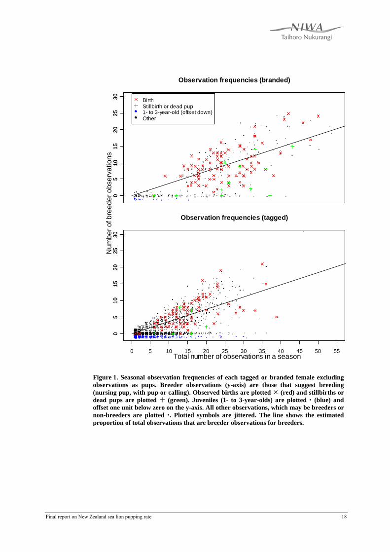
Figure 1. Seasonal observation frequencies of each tagged or branded female excluding observations as pups. Breeder observations (y-axis) are those that suggest breeding (nursing pup, with pup or calling). Observed births are plotted (red) and stillbirths or dead pups are plotted (green). Juveniles (1- to 3-year-olds) are plotted (blue) and offset one unit below zero on the y-axis. All other observations, which may be breeders or non-breeders are plotted . Plotted symbols are jittered. The line shows the estimated proportion of total observations that are breeder observations for breeders.


Births incl dead(branded)

05

1015 N = 97

Mean = 25.82CV = 0.32

Breeder obs >0(branded)

05

1015

2025

30

N = 216Mean = 25.76

CV = 0.38

3-year-old(branded)

01

23

45

6

N = 13Mean = 5.85

CV = 0.96

0 10 20 30 40 50 60

Births & brandings(tagged)

05

1015

N = 138Mean = 13.13

CV = 0.56

Breeder obs >0

05

1015

20 N = 727Mean = 11.7

CV = 0.65

3-year-old(tagged)

020

4060

80 N = 213Mean = 4.94

CV = 0.97

0 10 20 30 40 50 60Total number of observations in a season

Freq

uenc

y of

obs

erva

tions

Figure 2. Observation frequencies of tagged or branded females. Top row are definite breeders; second row are cows that have at least one breeder observation and are therefore almost all breeders; bottom row are 3-year-olds that are too young to breed but at least some of whom are receptive to males. The dashed vertical line is the mean.


5 10 15 20

0.0

0.2

0.4

0.6

0.8

1.0

( )

Age

Pro

porti

on o

f obs

erva

tions

that

sat

isfy

crit

erio

nPREVIOUS SEASONAll (N=2568)Pupped (N=703)Seen, no pup (N=789)Not seen (N=813)

Figure 3. Pupping rates estimated not using the model as the ratio of breeders to total cows known to be alive by age. Breeders are defined here as those cows that had at least one breeder observation. The solid line is the population mean. The dashed line is of those cows that bred in the previous season; the dotted line is of those that were seen the previous season but not identified as breeders; and the dot-dash line is of those that were not seen the previous season.


0 5 10 15 20

0.0

0.2

0.4

0.6

0.8

1.0

Age

Sur

viva

l

Model19871990199119921993199819992000200120022003

Figure 4. Survival rates (including retention of at least one tag or brand) by age for each cohort and as a population mean. The estimate for each cohort is made not using the model, as the ratio of cows known to be alive in one season to those in the previous season. The population estimate is from the model. Survival of pups is plotted as the mean of the cohort survivals.


02

46

1987N=18

Nf it=17.6Known N0=10

N0f it=14.3Mean obs=9.9

Mean f it=8.9

05

1020

1990N=114


N0f it=62.5Mean obs=12Mean f it=10.2

010

30

1991N=222



Mean f it=10.70

2040

1992N=380



Mean f it=10.8

010

30

1993N=352



Mean f it=10.9

020

60

1998N=182



Mean f it=8.8

020

4060

1999N=270



Mean f it=8.4

010

2030

40

2000N=199



Mean f it=8.3

020

4060

2001N=241

Nf it=233Known N0=115


Mean f it=7.4

0 20 40 60

05

1525

2002N=97



Mean f it=6.9

0 20 40 60

010

2030

2003N=138

Nf it=135Known N0=23


Mean f it=6.6

0 20 40 60Count

Freq

uenc

y of

tota

l obs

erva

tions

Figure 5. Total frequency counts by tagged cohort, observed (points) and predicted (lines). ‘N’ and ‘Nfit’ denote the observed and fitted number of observations; ‘Known N0’ and ‘N0fit’ denote the known number of live but unobserved animals (zeros) and the fitted number; ‘Mean obs’ and ‘Mean fit’ denote the observed and fitted distribution means. We expect ‘N0fit’ to exceed ‘Known N0’ because not all live animals are subsequently resighted. The difference is greater for the most recent cohorts.


05

1020

30

2000N=202



Mean f it=6.9

010

2030

40

2001N=199



Mean f it=8.7

010

2030

2002N=223



Mean f it=100

2040

6080

2003N=285



Mean f it=11.2

020

4060

80

2004N=320



Mean f it=10.3

010

2030

4050

2005N=293



Mean f it=8.5

0 20 40 60

020

4060

80

2006N=338



Mean f it=8.1

0 20 40 60

020

4060

2007N=353

Nf it=349.2Known N0=0N0f it=261.1

Mean obs=9.5Mean f it=9.7

0 20 40 60Count

Freq

uenc

y of

tota

l obs

erva

tions

Figure 6. Total frequency counts by observation season, observed (points) and predicted (lines). ‘N’ and ‘Nfit’ denote the observed and fitted number of observations; ‘Known N0’ and ‘N0fit’ denote the known number of live but unobserved animals (zeros) and the fitted number; ‘Mean obs’ and ‘Mean fit’ denote the observed and fitted distribution means. We expect ‘N0fit’ to exceed ‘Known N0’ because not all live animals are subsequently resighted. The difference is greater for the 2007 season.


02

46

8

1987N=18

Nf it=17.6Mean obs=3.7

Mean f it=2.4

010

30

1990N=114


Mean f it=3.1

020

4060

80

1991N=222

Nf it=212.1Mean obs=4Mean f it=3.3

040

8012

0

1992N=380


Mean f it=3.3

040

8012

0

1993N=352


Mean f it=3.3

040

8012

0

1998N=182


Mean f it=1.9

050

150

1999N=270


Mean f it=1.6

050

100

150 2000

N=199Nf it=197.2


050

150

2001N=241

Nf it=233Mean obs=1.4

Mean f it=0.9

0 5 15 25

020

60

2002N=97


Mean f it=0.6

0 5 15 25

040

8012

0

2003N=138

Nf it=135Mean obs=0.3

Mean f it=0.3

0 5 15 25Count

Freq

uenc

y of

bre

eder

obs

erva

tions

Figure 7. Breeder frequency counts by tagged cohort, observed (points) and predicted (lines). ‘N’ and ‘Nfit’ denote the observed and fitted number of observations; ‘Mean obs’ and ‘Mean fit’ denote the observed and fitted distribution means. The plots include a mixture of breeders and non-breeders.


020

4060

2000

N=202Nf it=165.8


020

4060

80

2001

N=199Nf it=194.5


020

6010

0

2002

N=223Nf it=233.3


050

100

150

2003

N=285Nf it=272.4


050

100

150

200

2004

N=320Nf it=312.3


050

100

150

200 2005

N=293Nf it=293.4


0 5 15 25

050

100

200

2006N=338


Mean f it=1.6

0 5 15 25

050

100

150

200

2007N=353


Mean f it=2.3

0 5 15 25Count

Freq

uenc

y of

bre

eder

obs

erva

tions

Figure 8. Breeder frequency counts by observation season, observed (points) and predicted (lines). ‘N’ and ‘Nfit’ denote the observed and fitted number of observations; ‘Mean obs’ and ‘Mean fit’ denote the observed and fitted distribution means. The plots include a mixture of breeders and non-breeders.


0 2 4 6 8 10 12 14 16 18 20

0.0

0.1

0.2

0.3

0.4

0.5

0.6

0.7

0.8

0.9

1.0

Age

Pro

babi

lity

Population meanPup previous yearNo pup previous yearPreliminary population mean

Figure 9. Pupping rate (probability of giving birth) by age. The estimated rate for cows that did not breed in the previous season (dashed line) is a constant proportion (33%) of that of those that did (thin solid line). The population mean (heavy line) is obtained iteratively from the other two functions. The preliminary population estimate from Figure 3 is repeated (dot-dashed line).


Final report on New Zealand sea lion pupping rate

Documents

Transcript of Final report on New Zealand sea lion pupping rate