FINAL REPORT Key comparison...

1

FINAL REPORT

Key comparison EUROMET.M.P-K1.a

Euromet project 442 A

Pressure range: 0.1 Pa – 1000 Pa Anita Calcatelli1, Fredrik Arrhen2, Mercede Bergoglio1, John Greenwood3, Rifat Kangi4, Karl Jousten5, Jean Claude Legras6, Markuu Rantanen7, Jos Verbeek8, Carmen Matilla Vicente9, Denes Szaulich10

December 2004

1 IMGC-CNR, Istituto di Metrologia G. Colonnetti, strada delle Cacce 73, 10135 Torino, Italy 2 SP, Swedish National Testing and Research Institute, Box 857, SE- 50115, Boras, Sweden 3 NPL, National Physical Laboratory, Hampton Road, Teddington, Middlesex, TW11 0LW, United Kingdom 4 UME, TUBITAK - Ulusal Metroloji Enstitusu (UME), Gebze, 41470, Kocaeli, Turkey; 5 PTB, Physikalisch-Technische Bundesanstalt (PTB), Abbestr. 2-12, 10587 Berlin, Germany 6 BNM-LNE, Bureau National de Metrologie-Laboratoire national d’Essais, 1 rue Gastone Boissier, 75724 Paris Cedex 75, france 7 MIKES, Centre for Metrology and Accreditation, P.O. Box 239, Lönnrotinkatu 37, FI-00181 Helsinki, Finland 8 NMi, NMi Van Swinden Laboratorium BV., Schoemakerstraat 97, P.O. Box 54, NL – 2600 AR Delft, The Netherlands 9 CEM, Centro Espanol de Metrologia, Calle de Alfar n. 2, 28760 Tres Cantos, Madrid, Spain 10 OMH, Országos Mérésügyi Hivatal (National Office of Measures), Németvölgyi út 37-39, H-1124 Budapest, Hungary

2

Content 1. Introduction 3 2. Participating laboratories and their standard systems 3 2.1 Independent standards 3 2.1.1 IMGC-CNR system 3 2.1.2 BNM-LNE 3 2.1.3 PTB system 4 2.1.4 NPL-UK system 4 2.1.5 UME system 5 2.1.6 OMH system B (from 10 Pa to 100 Pa) 5 2.2 Secondary systems equipped with transfer gauges 5 2.2.1 Mikes system 5 2.2.2 SP system 5 2.2.3 CEM system 5 2.2.4 OMH system A 6 2.2.5 NMi system 6 3. Transfer standards 6 4. Oganization of the EUROMET.M.P-K1.a comparison 7 4.1 Chronology of the measurements 7 4.2 General calibration procedure 7 4.3 Data presentation by the participating laboratories 8 5. Problems 8 6. Data handling at the pilot laboratory 8 6.1 Correction for the readings at base pressure 9 6.2 Correction for temperature 9 6.3 Calibration ratios 9 6.4 Uncertainty of the calibration ratios 10 6.5 Results- calibration ratios and their uncertainties 12 7. Evaluation of the comparison results 14 7.1 Predicted gauge readings and common reference values 14 7.2 Differences of pi,j from pri 15 7.3 Calculation of the uncertainty of the involved quantities 15 7.4 Degree of equivalence 16 7.5 Tables of the comparison results 17 8. Link with CCM.P-K4 comparison 20 9. References 25

3

1. Introduction

At a workshop held at NPL (UK) on 8th October 1997 it was decided that there should be a Europewide comparison in the absolute pressure range (0.1 – 1000) Pa with the main objective of having a set of laboratories, at regional level, connected to each other by a wide comparison in the most commonly required range for calibration in low pressure applications; in that comparison each participating laboratory could perform the calibrations by using its own reference system even if it was of a secondary type, provided it was traceable to known primary devices The transfer standards were commercially available capacitance diaphragm gauges (CDGs), prepared for the comparison by BNM-LNE (Fr) and IMGC-CNR (It) that was the pilot laboratory and the comparison was made under the EUROMET project 442 A coordinated by J.C. Legras of BNM-LNE. 2. Participating laboratories and their standard systems Twelve laboratories participated in the comparison and received the transfer gauges. Of these one laboratory, SMU did not return any results and another, CMI, informed the pilot laboratory before data circulation that its results had to be withdrawn; so that ten NMIs11 were included in the final evaluation. Tables 1 shows the list of the laboratories that participated in the comparison and kept the two packages for the agreed time interval (six weeks plus fifteen days for data preparation and checking). The following standards were used by the various participating laboratories:

- Six independent systems; four systems of the static expansion type and one based on pressure balances, one ultrasound manometer [for the (30-1000) Pa range only];

- Six systems equipped with gauges traceable to another primary laboratory [one laboratory only in the (0.1-30) Pa range]..

2.1 Independent standards 2.1.1 IMGC-CNR system The system consists of three volumes, nominally 10 mL, 500 mL and 50 L, the largest volume being the calibration chamber. The different expansion ratios are measured, and are periodically determined, by application of the multiple expansion method. The initial pressures between 1 kPa and 100 kPa are measured by secondary transfer standards directly traced to the HG5 mercury manometer. The base pressure, obtained by a turbo pump, is in the 10-6 Pa range /1/. 2.1.2 BNM-LNE system The BNM-LNE standard /2/ consists of a combination of three differential capacitance diaphragm gauges, respectively spanning the ranges 0.1 Pa to 100 Pa, 10 Pa to 1000 Pa and 1 kPa to 10 kPa. All the instruments to be compared are connected symmetrically to a vacuum chamber. The CDGs were initially calibrated at a line pressure near 50 kPa by comparison with two primary pressure balances, with nominal effective area of 20 cm2. Their reference chambers were then evacuated using a turbomolecular pump. The thermal transpiration effect is corrected by using the Takaishi and Sensui /3/ formulae with the experimentally determined sensor temperature.

11 NMI= National Metrology Institute

4

Table 1. Laboratories that received and kept the transfer standards for the time scheduled for the comparison NMI

Country

Reference system

Notes /CMC presence

IMGC-CNR Italy Static expansion system Independent - participated in the CCM.P-K 4/yes BNM-LNE France Pressure balance and transfer gauges (CDGs)

Independent/yes

MIKES

Finnland Transfer gauges Traced to PTB through a German accredited laboratory/yes

SP

Sweden

Transfer gauges

Traced to BNM-LNE/yes

PTB

Germany

Static expansion system

Independent- participated in the CCM.P-K 4/yes

CEM

Spain

Transfer gauges (CDGs)

Traced to NPL/yes

NPL

United Kingdom


Independent- participated in the CCM.P-K 4/yes

OMH

Hungary

System A: transfer gauges (0,1Pa-10 Pa); System B: ultrasound manometer (30 Pa-1000Pa)

(0,1 – 10) Pa traced to PTB; (30 – 1000) Pa independent/yes

UME

Turkey


Independent /yes

NMi

The Netherlands

Transfer gauges

Traced to PTB/ no

The calibration of the CDGs is performed for their analogue output signal, with a resolution of 0.01 mV. The modelling of the pressure versus the output signal, and the estimation of the stability of the instruments is based on a historical record spanning 10 years. The consistency between the 3 CDG was checked in their common ranges. The validity of the method at low pressure was demonstrated in the range 1x10-3 Pa to 100 Pa using the static expansion method: the consistency of a quartz gauge, a CDG and two spinning rotor gauges was inside 0.2 %. 2.1.3 PTB system The PTB primary standard is a static expansion system, called SE2, in which pressures are generated by expanding gas of known pressure from two alternative small volumes of nominally 0.1 L and 1 L directly into a volume of 100 L. It is also possible to carry out two expansions in series with intermediate nominal volumes of 100 L and 1 L. The regular operational range of SE2 is 0,1 Pa up to 1 kPa. The system is described in detail in references /4,5/. 2.1.4 NPL system The medium vacuum standard (SEA III) at the NPL is a three-stage non bakeable static expansion system with a 50 L calibration chamber. By varying the initial pressure and the number of stages of expansion, calculable pressures between 1.5×10-2 Pa and 2×103 Pa may be generated. There is a choice of two small vessels from which gas may be expanded into the calibration chamber and this enables a greater range of pressures to be generated from a given range of initial pressures. The

5

pressure of the initial gas sample is measured using a quartz Bourdon tube gauge. The pressure generated is calculated from knowledge of the initial pressure, the ratio of the volumes and the gas temperatures. The ratios of the volumes are determined using Elliott’s /6/ experimental procedure of repeated expansions and are calculated using the iterative method described by Redgrave et al /7/. 2.1.5 UME system A newly constructed multi-stage static expansion system has been used to generate calibration pressures in the range from 1×10-1 Pa up to 1×102 Pa. The apparatus consists of 6 vessels that provide a pressure reduction by a factor of about 10-6 in the main calibration vessel after three-step expansion. 17 platinum resistance thermometers that are mounted on the vessels are used for temperature corrections. The initial pressure before the first expansion is measured by an absolute quartz Bourdon helical gauge (Ruska DPG 7000) having 172 kPa full scale. The whole apparatus is built using UHV techniques and can be baked up to 400° C. 2.1.6 OMH system B (from 30 Pa to 100Pa) For the (30 –100) Pa pressure range the reference system (named B) is a modified ultrasonic mercury barometer. The original system, built by Dr Alfred Müller, was called EB3, (0…1150) mbar. The tubes were changed in 1993 from 14 mm inner diameter to 27 mm (to reduce uncertainty caused by variations in capillary depression). The height of mercury column is measured by the original ultrasonic system, but the velocity of sound in mercury is calculated using an equation published by NIST. The densities of mercury and air are calculated by formulae published in Metrologia /8/. 2.2 Secondary systems equipped with transfer gauges 2.2.1 MIKES system Two CGDs: 1 torr and 10 torr full scale MKS type 690 Baratrons were used in the comparison. They were calibrated in the accredited laboratory of MKS Munich in May 1999. The next calibration in April 2000 in the same laboratory showed that there were no problems with stability. Since 2002 the MIKES standards for this pressure range are a spinning rotor gauge, traced to NPL, and a force balanced piston gauge (model FPG8601 by DH Instruments) whose effective area is traced to BNM-LNE. 2.2.2 SP system The standards used were two CDGs, 1 torr and 100 torr full scale MKS type 390A Baratrons. They were calibrated at SP against two differential CDGs, 1 torr and 100 torr full scale MKS type 398 HD Baratrons that, in turn, were calibrated (at SP) against two RUSKA 2465 piston gauge standards calibrated at BNM- LNE. The reference side pressure, for the calibration of the absolute CDGs was measured with a MKS SRG-2, calibrated at NPL. The CDGs have been in use since 1992 and have shown good stability. 2.2.3 CEM System The CEM’s laboratory pressure standard is based on the dynamic expansion method, although during this intercomparison the set of calibrations were performed by direct comparison to MKS Baratron capacitance diaphragm gauges traceable to NPL, which were used as CEM’s standards. Their indications, the temperature of the calibration system and the indication of the transfer standard used in this comparison were recorded. An ionisation gauge and a spinning rotor gauge, checking the agreement of both readings within the uncertainties interval, determined the base pressure. An auxiliary turbo pump was used for the calibration of the 100 Pa differential CDG (Sensor 1, Table 2).

6

2.2.4. OMH system A For the (0,1 … 10) Pa pressure range a reference system named A is used in which a spinning rotor gauge (Leybold Vakuum GmbH/Viscovac VM211) calibrated by PTB is used to measure the generated pressure. Vacuum conditions are produced by a TRIVAC D1, 6B type two stage rotary pump and a type TURBOVAC 50 turbomolecular pump. A unique chamber is used for this standard and that described in 2.1.6. The volume of the chamber together with connecting pipes and valves used in normal intercomparisons is about 3 L, the typical rate of change in pressure is about Q = (2…6)×10-6 mbar L s-1.The zero base pressure was measured by a spinning rotor gauge. 2.2.5 NMi system The vacuum calibration facility of the NMi VSL consists of a non-bakeable vacuum chamber developed according to the DIN 28418 standard and a set of capacitance diaphragm gauges. For the lowest part of the calibration range a spinning rotor gauge is used. To reach an appropriate base vacuum pressure a turbo-molecular pump in combination with a two-stage oil rotary vacuum pump is used. The range of the calibration facility is from 1×10-6 hPa to 1000 hPa and is mainly used for the calibration of thermal conductivity gauges and diaphragm gauges. The claimed best measurement capability of the NMi VSL vacuum calibration facility in the range of the transfer standards is 0.04 + 0.002×p/Pa. The vacuum reference standards are traceable to PTB. 3. Transfer standards The transfer standards; consisting of three MKS Baratron sensors, two MKS Signal Conditioners and three cables, were operated in the configuration shown in Table 2. The absolute sensors (s2, s3) were provided with their own isolation valve; the differential sensor (s1) to be used in absolute mode was connected to two valves (v1 for pumping the reference side, v2 being a valve isolating the two sides of the sensor). The three sensors were not connected to each other because it was decided to let each participating laboratory be free to mount the gauges according to their usual practice. Table 2: Configuration details of the transfer standards Sensor Type Serial n FS range Controller, type, s/n Package 1 (s1) 698A01TRA 1060661140A 1 torr, differential 1; 670AD21,s/n 95170207A Provided by IMGC-CNR

2 (s2) 690A01TRB 24853 1 torr, absolute 2; 270DD-5, s/n 24851 SPF Provided by BNM-LNE

3 (s3) 690A11TRB 000188946 10 torr, absolute 1; 670D21,s/n 95170207A Provided by IMGC-CNR

The transfer gauges were circulated in two packages: One package provided by BNM-LNE contained a sensor head marked ‘Sensor 2’ (with a valve) and its own control unit marked ‘Control 2’, cable marked ‘Cable 2’ and shipping documents (ATA carnet for non EU countries). The second package provided by IMGC-CNR contained: a sensor head marked ‘Sensor 1’connected to an ion pump through valves and related pipes; a sensor head marked ‘Sensor 3’ with valve, control unit marked ‘Control 1’, cables marked ‘Cable 1’ and ‘Cable 3’,control unit for the ion pump and connecting cable, shipping documents (ATA carnet for non EU countries), instruction manual for sensor heads, instruction manual for the control unit, instruction manual for ion pump and control unit and a copy of the agreed protocol. All the CDGs were equipped with built-in heaters.

7

4. Organization of the EUROMET.M.P-K1.a comparison 4.1 Chronology of the measurements Table 3 shows the chronology of the measurements performed at the various participating laboratories. At the beginning twelve laboratories were scheduled for the comparison and they kept the packages for the planned period. At the end of the comparison data were made available by ten NMIs for the final evaluation. Table 3: Dates of the three calibrations performed at each NMI and at IMGC-CNR Laboratory Sensor 1 Sensor 2 Sensor 3 IMGC-CNR (IMGC1) 1998/09/29-30;1999/02/04 1998/11/25-27;1999/02/02 1998/12/12-14;1999/02/05 BNM-LNE 1999/03/09-10-11 1999/03/09-10-11 1999/03/16-17-18 MIKES 1999/08/26;1999/09/08-09 1999/08/26;1999/08-09 1999/08/20-23-24 IMGC-CNR (IMGC2) 1999/11/17-18-19 1999/11/01-05-08 1999/12/11-14-15 SP 2000/01/24-25-26 1999/12/22-29;2000/01-11 2000/01/18-19-20 PTB 2000/02/14-15-16 2000/02/14-15-16 2000/02/18-21-22 IMGC-CNR (IMGC3) 2000/04/11-12-13 2000/03/29-30-31 2000/04/04-05-06-10 CEM 2000/06/05-06-07 2000/05/19-23-29 2000/06/09-12-13

Repair and controls on all the sensors IMGC-CNR (IMGC4) 2000/10/27-30-31 2000/12/04-05-06 2000/11/14-15-20 NPL 2001/01/22-23-24 2001/01/25-26-27 2001/01/17-18-19 IMGC-CNR (IMGC5) 2001/07/26-27-28 2001/07/20-23-24 No longer available OMH 2001/03/14-19-20 2001/04/09-11-12 No longer available UME 2001/10/31;2001/11/01-02 2001/11/08-09-11-12 NMi 2002/02/07 2002/02/05 IMGC-CNR (IMGC6) 2002/05/06-07-08 2002/04/19-22-23 4.2 General calibration procedure Sensors had to be connected by means of suitable pipes to the reference system of the participating laboratory and mounted with the base plate as horizontal as possible. The valves had to be operated following the technical protocol of the comparison. All the participating laboratories had a good knowledge of the CDG sensors and control units, so that no special instructions were given. The control unit and the heating had to be switched on at least 48 hours before starting the calibrations. Both the control units had to be operated with the range selection in the position ×1 except for the lowest pressure range (0.1 Pa and 0.3 Pa) where the range selector had to be in the ×0.1 position. All the sensors were calibrated using the display of the signal conditioners. The calibration runs were performed in nitrogen. Before starting the calibration, NULL and FS indications had to be adjusted; at the lowest pressure, the gauges had to be checked for zero reading, but not adjusted, following the specific conditions given in the technical protocol. Following the protocol, the zero reading of the transfer gauges had to be measured before and after each calibration run and at each pressure level when possible. The calibrations were performed in the range from 0.1 Pa to 1000 Pa at the following pressure values:

8

0.1 Pa, 0.3 Pa, 1 Pa, 3 Pa, 10 Pa, 30 Pa, 100 Pa for s1 and s2 (1 torr full scale). 0.1 Pa, 0.3 Pa, 1 Pa, 3 Pa, 10 Pa, 30 Pa, 100 Pa, 300 Pa, 1000 Pa for s3 (10 torr full scale). The generated pressure values had to be as close as possible to indicated target pressure (at least within 2%). At each pressure value the participating NMIs had to provide three sets of: generated pressures of the reference standard and their standard uncertainties, the readings of the gauges, the values of the calibration vessel temperature. Three complete calibration runs were performed, preferably on three different days. Due to the problems described in Sec. 5, six complete sets of calibrations were performed at IMGC-CNR for the sensors s1 and s2 while for the sensor s3 there were four. 4.3.Data presentation by the participating laboratories

The generated pressure values with their standard uncertainties corresponding to the nominal values (pt), the gauges readings (at the base and at generated pressures) and the temperature of the calibration vessel were recorded on Excel sheets and sent to the pilot laboratory. 5. Problems Initially it was intended that the sensor s1 could be operated with its reference side pumped by the ion pump included in package 1, while each participating laboratory should provide a roughing pump. However, in the middle of the comparison, the ion pump was left exposed to the atmosphere for a long time and became heavily contaminated. Consequently it was decided to proceed without the ion pump and each NMI had then to provide a pumping system for the reference side of that sensor (beginning at CEM). On the way from CEM to NPL all the sensors suffered serious damage. One package was sent back to BNM-LNE and the second one to IMGC-CNR for inspection and repair. Evidently the bodies of the gauges were twisted and the pipes disconnected from the heads. All the gauges were welded at IMGC-CNR (s1 and s3) and at BNM-LNE (s2) and kept under control to check their operational behavior; finally all the three transfer gauges were calibrated again at IMGC-CNR. After several calibration cycles it was decided to proceed with the comparison because the characteristics of the sensors were comparable with those shown before they were damaged, although the range of sensor s3 had to be reduced to 3 Pa at its lower limit. The two packages were sent again to NPL and the transfer gauges were calibrated there; after that the two packages were sent to OMH. On arrival at OMH s3 was found to be damaged again. Considering that the comparison time schedule was already increased, IMGC-CNR decided to continue the comparison at the other laboratories with only the remaining transfer gauges, s1 and s2, which were shipped by OMH to SMU, then to IMGC-CNR, UME and NMi. The damage to the transfer standards caused a shift in the time schedule and consequently the ATA carnets expired and had to be renewed twice. 6. Data handling at the pilot laboratory

All the data from the various NMIs were checked and evaluated at the pilot laboratory in terms of calibration ratios, given by the ratio of the gauge readings to the generated/measured pressure appropriately corrected as regards zero reading and temperature.

9

6.1 Correction for the readings at base pressure The NMIs equipped with primary systems provided the generated pressures without the need for any correction for the base pressure which was negligible low; so that only the readings of the transfer gauges had to be corrected for the zero readings. For those NMIs the mean zero reading was subtracted from the gauge readings at the target. For the data provided by NMIs equipped with secondary reference gauges both the generated/measured pressures and transfer gauge readings were corrected for their own average zero readings. 6.2 Correction for temperature Following the protocol all the transfer gauges were operated with their heaters switched on, so that their operation temperature was always close to 45 °C, while the temperature of the standards to which the gauges were connected ranged from 19 °C to 23 °C. To determine the temperature of the heads several tests were performed at IMGC-CNR to find the most probable temperature of the sensors when in operation. In particular, sensor s2 was calibrated with its heater first switched on then off but with the head located in a climatic cell in which the temperature could be changed, controlled (at ± 7× 10-2 °C) and measured. Comparing the curves of the calibration ratio versus the pressure it was decided that, in general, 45 °C could be considered as the real average working temperature. Although several fitting curves have been reported /9,10/ that take into account the different temperatures of the calibration systems and “linearize” the curve of the calibration ratio as a function of the pressure, it was decided to apply the fitting formula presented first in /3,11/ as it was applied to the data of the CCM comparison CCM.P-K4 /12/. The effect of the different operating temperatures was minimized by determining the pressure that a primary or reference standard would generate/measure if it was operating at the same temperature as the transfer standard gauges by the following relationship:

ps,h,l,i,j = (ps,h,l,i,j)listed . [aY2 + bY+cY0.5 + 1]/[aY2 + bY + cY 0.5 + (Ts,h,,l,i,j/Tg,h,,l,i,j)0.5] [1] where s stands for standard and g for gauge; i for pressure level and j for the considered laboratory, h for repeated measurements (9) and l for the considered gauges (1,2, 3, corresponding to s1, s2 and s3). Y is given by:Y=2ps,h,l,i,jd/[133(Ts,h,l,i,j+Tg,h,l,i,j)], where Ts,h,l,i,j and Tg,h,l,i,j are the absolute temperatures respectively of the standard and of the gauge to be calibrated; (ps,h,l,i,j)listed is the generated pressure in the reference system as determined by each participating NMI. The remaining quantities are: internal diameter of the gauge inlet tube d= 4.6 mm and, for nitrogen: a = 1.2 × 106 K2 torr-2 mm-2, b = 1.0 × 103 K torr-1mm-1, c = 14 K0.5 torr-0.5mm-0.5/3,10/. As the empirical formula [1] was applied for the nominal 45 °C gauge temperature it should be noted that the precise uncertainty of the method is not known. However, since the correction is applied to all the data from all the involved laboratories at each pressure level and for repeated measurements, the contribution of the fitting curve to the uncertainty is disregarded (see also ref./12/). 6.3 Calibration ratios The calibration ratios (Fc) have been evaluated by the ratio of the transfer gauge readings (pg,h,l,i,j) to the standard pressures (ps,h,l,i,j) as corrected by [1]. When necessary, both pg,h,l,i,j and ps h,l,i,j have been corrected for zero readings. At each target pressure pti and for each transfer gauge the mean values of the nine Fch,l,i,j has been calculated as:

10

( )( )

9 9 9g ,h,l ,i, j g ,h,l ,i, j zero g ,h,l ,i, jlistedl ,i, j h,l ,i, j

h 1 h 1 h 1 s,h,l ,i, js,h,l ,i, j s,h,l ,i, j zero corr

p ( p ) p1 1 1Fc Fc9 9 9 pp ( p )= = =

−= = =∑ ∑ ∑

− [2]

So that for each participating laboratory seven values of Fcl,i,j and its relative standard deviation are derived for s1 and s2 transfer gauges and, in general and when possible, nine values for s3 transfer gauge. To have, at each pressure level, only one set of gauge factors for IMGC-CNR the average of the mean values of the six calibration sets for s1 and s2 and of four calibration sets for s3 has been evaluated:

6l ,i,IMGC CNR l ,i,IMGC CNR,k

k 1

1Fc Fc6− −

== ∑

[3] 4

3,i,IMGC CNR 3,i,IMGC CNR,kk 1

1Fc Fc4− −

== ∑

6.4 Uncertainty of the calibration ratios

The relative combined variance of each calibration ratio is given by:

( ) ( ) ( )2 2 22 2r l ,i , j rst l ,i , j rlts l ,i , j rstr l ,i , j rresol l ,i , ju ( Fc ) u ( Fc ) u Fc u Fc u Fc = + + + +

( ) ( )2 2r ,zero l ,i , j r ,T l ,i , ju Fc u Fc + + [4]

Where: urst is the relative uncertainty quoted by each NMI for its standard, as indicated in Table 4. The uncertainty of the standard reading at the base pressure is taken into account when necessary. urlts is the relative uncertainty due to long term instability. Since there is no evidence of continuous systematic shift of the gauge factors in the various calibrations performed at IMGC-CNR over the long calibration period, the relative uncertainty component due to long term instability of gauge factors (as determined by [2]) is evaluated for the s1 and s2 sensors by the six sets of calibrations performed at IMGC-CNR for the whole comparison period and is given, for s3, by the four sets of calibration results. It is calculated by the half difference between the maximum and the minimum values of the Fci,l,IMGC-CNR as follows urlts = (1/2) [(Fcl,i,IMGC-CNR)max– (Fcl,i,IMGC-CNR )min] [5] where i is associated with the two highest pressure levels. The values obtained at 30 Pa and 100 Pa for s1 and s2 sensors, 300 Pa and 1000 Pa for s3 sensor are averaged. Those average values are considered as type B components and are applied to all the NMIs including the pilot laboratory at each pressure level. urstr is the relative uncertainty component due to short term repeatability of the calibration ratio in three runs performed at each NMI (i.e. for the nine values for each level of pressure). Even if there are some systematic effects evident for day-to-day calibration at the same laboratory it was decided to represent the repeatability by the standard deviation of the mean, since any other choice may be equally arbitrary.

11

Table 4: relative standard uncertainty values as quoted by each NMI for its reference standard

For the pilot laboratory, where Fc is evaluated from [3], the short-term repeatability is evaluated as follows:

( )− −=

= ∑

2 62 2rstr l ,i ,IMGC CNR rstr l ,i ,k ,IMGC CNR

k 1

1[ u ( Fc )] u Fc6

[6a] for sensors s1 and s2, and

( )− −=

= ∑

2 42 2rstr l ,i,IMGC CNR rstr l ,i,k ,IMGC CNR

k 1

1[u ( Fc )] u Fc4

[6b]

for the sensor s3. Since there are only nine values available for each laboratory at each pressure level the standard deviation of the mean is multiplied by the factor )3/()1( −− nn , that is by a factor 1.155 as suggested in /13/. urresol is the relative uncertainty component due to the resolution of the Signal Conditioners used with the sensors; the resolution of the zero readings at base pressure is also included; this component has been included for reason of completeness. ur,zero is the component due to the fluctuations and drift of the zero readings of the transfer gauges. For the majority of the NMIs the resolution covers the possible fluctuations of the zero readings. When the fluctuations are outside of the resolution a component of the uncertainty has been considered by taking the rectangular distribution and averaging among the various runs at each pressure level.12 This component is then considered as type B and added arithmetically to the resolution. ur,T is the component of the uncertainty due to the temperature of the primary or reference standards. The uncertainty with which the temperature of the standards is measured is not taken into account; however, applying equations [1] and [2] and assuming a reasonable value of 0.2°C, the relative contribution is less than 3x10-4 for pressures below 1 Pa and is in the region of 10-5 Pa for higher pressures.

12 Two NMIs (BNM-LNE and CEM) show a considerable fluctuation of the zero readings. For BNM-LNE the zero readings for all the transfer gauges show variations considerably outside of the resolutions while CEM has similar variations only for sensor 1.

NMI PTB BNM-LNEBNM-LNE MIKES SP IMGC-CNR CEM CEM NPL OMH OMH UME NMi

p t(Pa) (s1,s2) (s3) (s1,s2) (s3) (s1) (s2)

0.1 1.4E-03 6.0E-03 6.0E-03 1.9E-01 4.0E-02 2.1E-03 5.5E-03 9.4E-03 4.1E-03 5.7E-02 8.2E-02 5.2E-03 2.5E-01

0.3 1.2E-03 2.7E-03 3.0E-03 6.8E-02 2.4E-02 2.0E-03 4.4E-03 8.4E-03 4.0E-03 2.7E-02 3.3E-02 3.8E-03 8.4E-02

1 1.1E-03 1.8E-03 2.0E-03 2.2E-02 1.9E-02 1.9E-03 3.2E-03 6.2E-03 3.0E-03 4.0E-02 4.1E-02 3.8E-03 2.6E-02

3 1.0E-03 1.3E-03 1.5E-03 8.2E-03 1.1E-02 1.1E-03 3.1E-03 6.1E-03 3.0E-03 4.0E-02 4.0E-02 3.8E-03 9.3E-03

10 9.0E-04 5.7E-04 8.8E-04 3.4E-03 6.1E-03 8.2E-04 3.1E-03 6.1E-03 3.0E-03 5.0E-02 4.0E-02 3.8E-03 3.5E-03

30 7.0E-04 2.3E-04 7.0E-04 2.4E-03 4.7E-03 8.5E-04 2.5E-03 2.0E-03 1.8E-03 5.0E-02 5.0E-02 2.6E-03 1.8E-03

100 7.0E-04 2.0E-04 7.0E-04 2.1E-03 4.2E-03 8.4E-04 2.2E-03 1.9E-03 1.8E-03 1.5E-02 1.5E-02 2.6E-03 1.3E-03

300 7.5E-04 7.0E-04 2.0E-03 1.9E-03 8.3E-04 1.9E-03 1.8E-03

1000 8.0E-04 7.0E-04 2.0E-03 6.9E-04 8.3E-04 1.9E-03 1.8E-03

12

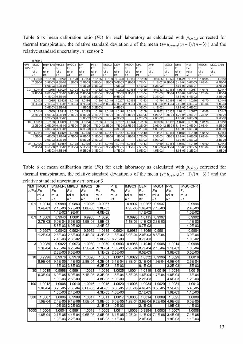
6.5 Results –calibration ratios and their uncertainties In the following tables more digits than are significant are given for the calibration ratios to facilitate the computation checks. Table 6 summarizes the results in terms of the average of the gauge factors for the various transfer gauges and for each NMI as calculated by the relationship [2] with ps,h,l,i,j corrected for thermal transpiration as described in Sec. 6.2 equation [1] and for the zero readings when necessary; the relative standard deviations s of the means and the relative combined standard uncertainty ur are also given. The IMGC-CNR data are average values, as for the other NMIs, and are related to six sets of calibrations for the sensors s1 and s2 and to four sets of calibrations for sensor s3. The last column of tables 6 are related to the average values for IMGC-CNR as calculated from equation [3] and the uncertainty values evaluated from the various components described in Sec. 6.4. Table 6 a: mean calibration ratio (Fc) for each laboratory as calculated with ps,h,l,i,j corrected for thermal transpiration, the relative standard deviation s of the mean (s= )3/()1( −− nnurstr ) and the relative standard uncertainty ur: sensor 1

sensor 1NMI IMGC1 BNM-LNEMIKES IMGC2 SP PTB IMGC3 CEM IMGC4 NPL OMH IMGC5 UME NMi IMGC6 IMGC-CNR pt/Pa F c Fc Fc Fc Fc Fc Fc Fc Fc Fc Fc Fc Fc Fc Fc Fc

rel s rel s rel s rel s rel s rel s rel s rel s rel s rel s rel s rel s rel s rel s rel s rel su r u r u r u r u r u r u r u r u r u r u r u r u r u r u r u r

0.1 0.9955 0.9872 1.0130 0.9967 0.9995 0.9986 0.9970 0.6794 0.9939 1.0010 0.5886 1.0016 1.0022 0.9449 1.0004 0.99751.4E-03 6.5E-03 3.0E-02 2.0E-03 1.6E-03 7.4E-04 1.2E-03 6.2E-02 1.7E-03 5.5E-04 3.2E-02 3.2E-04 4.7E-03 5.2E-03 7.1E-04 5.5E-04

1.1E-02 2.0E-01 4.0E-02 3.2E-03 6.2E-02 5.0E-03 6.5E-02 7.6E-03 2.5E-01 3.6E-030.3 0.9966 0.9927 1.0071 0.9946 0.9992 0.9995 0.9947 0.8949 0.9994 1.0000 1.0223 1.0006 1.0009 0.9783 0.9992 0.9975

1.1E-03 8.9E-04 7.1E-03 1.9E-04 8.5E-04 5.1E-04 2.4E-04 1.6E-02 2.0E-04 1.6E-04 8.0E-03 2.9E-04 5.0E-04 1.6E-03 2.4E-04 2.0E-044.3E-03 6.9E-02 2.4E-02 3.0E-03 1.7E-02 4.8E-03 2.8E-02 4.7E-03 8.4E-02 3.3E-03

1 0.9978 0.9932 1.0020 0.9955 1.0001 0.9999 0.9964 0.9984 0.9995 0.9999 0.9967 1.0006 1.0040 0.9976 0.9996 0.99834.5E-04 3.9E-04 3.5E-03 2.5E-04 2.6E-04 2.9E-04 1.4E-04 4.0E-03 7.1E-05 4.2E-04 3.3E-03 2.5E-04 4.9E-04 5.4E-04 1.0E-04 1.0E-04

3.4E-03 2.2E-02 1.9E-02 2.9E-03 5.8E-03 4.1E-03 4.1E-02 4.7E-03 2.6E-02 3.4E-033 0.9977 0.9953 0.9986 1.0001 1.0012 0.9997 0.9962 0.9997 1.0005 1.0007 0.9648 1.0009 1.0061 0.9856 1.0000 0.9992



2.7E-03 4.3E-03 6.7E-03 2.8E-03 4.1E-03 4.0E-03 5.0E-02 4.6E-03 4.4E-03 2.8E-0330 0.9986 1.0003 0.9999 1.0009 0.9998 1.0013 0.9995 1.0001 1.0037 1.0020 1.0364 1.0037 1.0058 1.0038 1.0022 1.0014



2.6E-03 4.1E-03 5.0E-03 2.7E-03 3.4E-03 3.2E-03 1.5E-02 3.7E-03 2.9E-03 2.8E-03

13

Table 6 b: mean calibration ratio (Fc) for each laboratory as calculated with ps,h,l,i,j corrected for thermal transpiration, the relative standard deviation s of the mean (s= )3/()1( −− nnurstr ) and the relative standard uncertainty ur: sensor 2

Table 6 c: mean calibration ratio (Fc) for each laboratory as calculated with ps,h,l,i,j corrected for thermal transpiration, the relative standard deviation s of the mean (s= )3/()1( −− nnurstr ) and the relative standard uncertainty ur: sensor 3

sensor 2NMI IMGC1 BNM-LNEMIKES IMGC2 SP PTB IMGC3 CEM IMGC4 NPL OMH IMGC5 UME NMi IMGC6 IMGC-CNR pt/Pa F c Fc Fc Fc Fc Fc Fc Fc Fc Fc Fc Fc Fc Fc Fc Fc

rel s rel s rel s rel s rel s rel s rel s rel s rel s rel s rel s rel s rel s rel s rel s rel su r u r u r u r u r u r u r u r u r u r u r u r u r u r u r u r

0.1 1.0103 1.0160 0.9733 1.0128 1.0114 1.0165 1.0199 1.0420 1.0155 1.0168 0.9625 1.0175 1.0224 1.0151 1.0185 1.01587.0E-04 3.9E-03 6.3E-03 1.8E-03 2.4E-03 5.8E-04 1.3E-03 3.0E-03 7.9E-04 1.7E-04 1.1E-02 8.8E-04 6.4E-04 3.6E-03 4.0E-04 4.4E-04

8.0E-03 1.9E-01 4.0E-02 3.4E-03 7.0E-03 5.1E-03 8.2E-02 6.0E-03 2.5E-01 3.7E-030.3 1.0113 1.0075 1.0027 1.0124 1.0164 1.0162 1.0145 1.0292 1.0163 1.0159 0.9783 1.0163 1.0218 1.0087 1.0175 1.0147



3.6E-03 2.2E-02 1.9E-02 3.2E-03 4.4E-03 4.3E-03 4.1E-02 4.9E-03 2.6E-02 3.6E-033 1.0114 1.0089 1.0114 1.0163 1.0179 1.0146 1.0140 1.0170 1.0147 1.0159 0.9882 1.0152 1.0210 1.0077 1.0168 1.0147



3.0E-03 4.5E-03 6.8E-03 3.1E-03 4.3E-03 4.2E-03 4.0E-02 4.8E-03 4.6E-03 3.1E-0330 1.0111 1.0118 1.0127 1.0149 1.0139 1.0150 1.0147 1.0147 1.0164 1.0149 1.1121 1.0163 1.0186 1.0179 1.0172 1.0151



2.9E-03 4.3E-03 5.2E-03 3.1E-03 3.7E-03 3.5E-03 1.5E-02 3.9E-03 3.2E-03 3.1E-03

NMI IMGC1 BNM-LNEMIKES IMGC2 SP PTB IMGC3 CEM IMGC4 NPL IMGC-CNR pt/Pa F c F c F c F c F c F c F c F c F c F c Fc

rel s rel s rel s rel s rel s rel s rel s rel s rel s rel s rel su r u r u r u r u r u r u r u r u r u r u r

0.1 1.0014 0.9989 0.9863 1.0026 0.9967 0.9997 1.0257 0.9937 0.99943.4E-03 2.1E-03 5.7E-03 1.8E-03 3.8E-03 4.9E-03 1.6E-03 7.1E-03 2.4E-03

1.4E-02 1.9E-01 4.0E-02 1.1E-02 1.0E-020.3 1.0009 0.9943 1.0001 0.9963 1.0026 0.9998 1.0115 0.9997 0.9992

2.7E-03 6.0E-04 6.6E-03 1.9E-03 1.9E-03 1.1E-03 1.1E-03 2.8E-03 1.1E-035.5E-03 6.9E-02 2.4E-02 8.7E-03 4.0E-03

1 0.9997 0.9842 0.9924 0.9972 1.0185 0.9924 0.9986 1.3069 0.9981 0.99841.2E-03 2.6E-03 2.5E-03 3.4E-04 4.2E-03 1.8E-03 3.0E-04 2.0E-03 8.8E-04 3.9E-04

7.4E-03 2.3E-02 2.0E-02 6.2E-03 8.7E-03 1.0E-023 0.9989 0.9922 0.9973 1.0030 1.0079 0.9993 0.9988 1.1040 0.9986 1.0014 0.9998

1.3E-04 4.2E-04 6.2E-04 1.5E-04 9.3E-04 1.0E-03 2.9E-04 8.7E-04 2.1E-04 1.1E-03 1.0E-042.8E-03 8.5E-03 1.1E-02 2.5E-03 6.5E-03 3.8E-03 3.5E-03

10 0.9996 0.9970 0.9979 1.0028 1.0031 1.0011 1.0022 1.0332 0.9996 1.0029 1.00108.9E-04 9.1E-05 1.1E-03 2.8E-04 4.2E-04 3.1E-04 3.8E-04 3.1E-04 1.9E-04 4.0E-04 2.6E-04

1.3E-03 3.6E-03 6.2E-03 1.3E-03 6.1E-03 3.2E-03 1.5E-0330 1.0015 0.9998 0.9991 1.0021 1.0016 1.0025 1.0004 1.0119 1.0019 1.0034 1.0015


100 1.0012 1.0008 1.0010 1.0016 1.0015 1.0020 1.0005 1.0034 1.0020 1.0031 1.00131.8E-04 3.2E-05 7.6E-04 6.6E-05 4.4E-05 3.8E-05 9.3E-05 4.6E-05 3.5E-05 3.5E-05 5.4E-05

1.0E-03 2.4E-03 4.3E-03 1.0E-03 2.1E-03 1.9E-03 1.1E-03300 1.0007 1.0006 0.9989 1.0017 1.0011 1.0017 1.0003 1.0014 1.0009 1.0025 1.0009


1000 1.0004 1.0004 0.9991 1.0018 1.0009 1.0011 1.0006 0.9994 1.0003 1.0007 1.00081.6E-04 2.7E-05 4.4E-04 9.6E-05 2.6E-05 6.1E-05 2.2E-04 1.1E-04 7.1E-06 3.4E-05 7.1E-05

1.0E-03 2.2E-03 1.0E-03 1.1E-03 2.0E-03 1.9E-03 1.1E-03

14

7. Evaluation of the comparison results

To evaluate the results of the comparison it is necessary to generate common reference values of the pressure at the various considered levels; then the differences of the pressures generated by each NMI with respect to the reference values can be evaluated with their uncertainties. Consequently, the following quantities must be defined and calculated so that the degree of equivalence can be evaluated for each NMI. 7.1 Predicted gauge readings and common reference values The calibration ratios (Fc), as calculated from [2] and [3] for all the NMIs, are used to calculate the values of the gauge readings that would have been measured if the reference standards had generated exactly the common hypothetical target pressures, that is pti /12/. Those gauge readings are evaluated by multiplying the calibration ratios Fcl,i,j by the target pressures as follows: pl,i,j = Fc l,i,j × pti [7] In the (0.1-100) Pa pressure range all the laboratories have calibrated two gauges (s1 and s2), while for the higher-pressure range not all the laboratories could perform the calibrations Sec. 5.) of gauge s3. Consequently up to 100 Pa there are two values of pressure gauge readings as calculated by [7] so that mean gauge readings are evaluated by simple arithmetic means /12/: [pi,j]1+2= (p1,i,j+p2,i,j)/2 [8a ] while for s3 pressure gauge readings are simply given by: [pi,j]3= Fc 3,i,j × pti [8b] For the pilot laboratory the mean values are evaluated from the three average values of all the loops as given by [3]. Common EUROMET comparison reference values pri at the target pressures pti, may be obtained by simple arithmetic means13 of the pi,j as deduced from the data of the five independent NMIs (IMGC-CNR, BNM-LNE, PTB, NPL, UME):

∑==

5

1,5

1j

jii ppr [9]

To have pri=pti, correction factors are required that are given by [fni]1+2 =pti/[pri]1+2, for sensors s1+s2 and [fni]3 =pti/[pri]3 for the gauge s3. To subsequently derive pi,j that would have been read at each NMI if the generated/measured pressure was exactly equal to the target pressure each [pi,j]1+2 and [pi,j]3 have to be multiplied by the fni factors: p1+2,i,j =[fni]1+2 . [pi,j]1+2 [10a] p3,i,j = [fni]3 . [pi,j]3 [10b] 13 From consistency checks (based on χ2) at 95% probability, the weighted and arithmetic means may be considered equivalent for sensors s1 and s2 while for sensor s3, in general, it seems better to avoid the weighted mean. The arithmetic mean has been adopted over the whole pressure range for reasons of harmonization with the treatment of the data in the CCM.P-K4 comparison to which the present comparison data is to be linked.

15

for the two sets of data regarding s1 and s2 together and s3. The same procedure is applied when the data for s1 and s2 gauges are treated separately. 7.2 Difference between pi,j and pri To compare the data, every mean pi,j value obtained for each laboratory and at each pressure is compared with pri through the difference given by /14,15/ ∆pi,j = pi,j - pri [11] 7.3 Calculation of the uncertainty of the involved quantities

Variances from the following sources have been considered /16/: predicted gauge reading (pl,i,j): the relative combined variance given by [4] is also the relative variance of pl,i,j as defined by [7]; so that the variance of the predicted gauge readings is obtained by multiplying the relative combined variance of Fcl,i,j by the target pressure pti. Using the relationship in [10], that variance is given by: u2(pl,i,j) = [pti fni ur( Fcl,i,j)]2 Since the terms fni may be considered as factors with zero uncertainty and values very near to one, the variance of pl,i.j is given by: u2(pl,i,j) = [pti ur( Fcl,i,j)]2 [12] mean values of pl,i,j: for the mean values of the sensors s1 and s2 as given by [8a] and [10a] correlations must be considered due to the fact that at each NMI the two sensors have been calibrated with the same standard system. They therefore have in common the component of the variance due to the standards. For the mean values of the two gauges s1 and s2 we have:

( ) ( )[ ] ),(21

212

41)

2()( ,,2,,1,,2

2,,1

2,,2,,12,

2jijijiji

jijiji ppupupu

ppupu

⋅

⋅++=

+= [13]

The correlation through the standard (Sec. F.1.2 ref. /16/, particularly Sec. F.1.2.3), is given by:

)()(),( ,,2,,1,,2,,1 jistjistjiji pupuppu ⋅=

hence

( ) ( )[ ] )()(21

41)(

,,2,,1,,2,,1

22,

2jijijiji

pupupupupu ststji ⋅

++= [14]

The two values ust(p1,i,j) and ust(p2,i,j) are considered separately because the pressure values may be different. If the relative uncertainty for the standard is considered the two values are equal. reference value pri: being pri calculated as the arithmetic mean of the five independent NMIs (IMGC-CNR, BNM-LNE, PTB, NPL and UME). Its variance is given by the average of the variance of the pi,j calculated for those laboratories:

16

( )∑=

=5

1,

22

251)(

jjii pupru [15]

difference ∆pi,j: from the definition given in [11], )( , jipu ∆2 is given by

)()( ,

2,

2ijiji prpupu −=∆

at each pressure level. For the correlation between pi,j and pri the following groups of NMIs must be considered differently: 1. IMGC-CNR, PTB, NPL, BNM- LNE, UME: pi,j and pri are correlated because pri is evaluated from

their data; 2. NMIs whose standards are traceable to another primary laboratory, as is the case for:

MIKES traced to PTB SP traced to BNM-LNE CEM traced to NPL OMH traced to PTB through an accredited German laboratory for the (0.1 – 10) Pa range and it is independent from the other NMIs for the (30 –100) Pa range NMi traced to PTB

For all the NMIs in 1. the correlation has been estimated as follows:

( ) ( ) ( )ijiijiijiji prpuprupuprpupu ,2)()]([ ,2

,2

,2

,2 −+=−=∆

( )[ ]

)(53)()]([

)(52)()(

,22

,2

,22

,2

,2

jiiji

jiijiji

puprupu

puprupupu

+=∆

−+=∆ [16]

Equation [16] has been obtained by considering, for the specific NMI, the correlation between pi,j and pri through the component of u(pri) due to that laboratory [u(pi,j)]. For the laboratories traced to one of five NMIs in group 1, the correlation is through their reference standards and that of the laboratory to which they are traceable. The variance of ∆pi,j (see Sec. F 1.2 of ref /15/) of the NMIs in group 2 is therefore estimated by:

),(252)(2),(2),(),(

52)(2),(2),((2

jipstuipruimpujipstujipstuipruimpuimpu −+=−+=∆ [17]

where m indicates one of the NMIs in group2 while j stands for PTB or BNM-LNE or NPL depending on the specific case. The term due to the correlation in [17] is considerably smaller than the other two components and it may be disregarded. The expanded uncertainty is then given by

( )[ ] ( )[ ]jiji pupU ,2

, 2 ∆⋅=∆ [18] for all the laboratories 7.4 Degree of equivalence

The degree of equivalence can be evaluated by considering of the differences ∆pi,j as given by [11], together with their expanded uncertainties U(∆(pi,j) as given by [18] since for equivalence the following conditions must be fulfilled

17

( )

1)(

)(,

,, ≤

∆

∆=∆

ji

jiji pU

pABSpE [19]

where E, as is usual, stands for normalized error. 7.5 Tables of the comparison results

The results of the comparison calculations are presented in tables 7 and 8. Each table shows, for each NMI, the gauge reading as evaluated by multiplying the calibration ratio by the target pressure (by applying the equations [7], [8], [9] and [10]); the related combined uncertainty values (as calculated by the equations [13] and [14]); the differences ∆pi,j (as calculated by using the relationships [11] with their expanded uncertainties as given by the equation [18] through [16] and [17]). The normalized errors as given by [19] are also listed to facilitate the analysis of the data. Table 7 relates to the combination of sensors s1 and s2 while table 8 is related to sensor s3.

Table 7: Laboratory values (pi,j) with their standard uncertainty u(pi,j), differences (∆pi,j) from pri with their expanded uncertainty U(∆(pi,j)) (k=2) and the normalized error values: combination of sensor s1 and s2.

NMI p t p i, j u (p i, j) ∆(p i, j) U (∆(p i, j)) Ei,j

Pa Pa Pa Pa Pa

IMGC-CNR 0.1 0.0999 3.0E-04 -7.4E-05 6.4E-04 1.1E-010.3 0.2998 8.5E-04 -1.7E-04 1.6E-03 1.1E-01

1 0.9992 2.9E-03 -7.7E-04 5.2E-03 1.5E-013 2.9981 7.0E-03 -1.9E-03 1.3E-02 1.4E-01

10 9.9928 2.2E-02 -7.2E-03 4.2E-02 1.7E-0130 29.9893 6.6E-02 -1.1E-02 1.2E-01 8.9E-02

100 99.9152 2.2E-01 -8.5E-02 4.0E-01 2.1E-01BNM-LNE 0.1 0.0994 8.0E-04 -5.8E-04 1.3E-03 4.4E-01

0.3 0.2980 1.1E-03 -2.0E-03 1.9E-03 1.0E+001 0.9937 2.8E-03 -6.3E-03 5.1E-03 1.2E+003 2.9835 7.2E-03 -1.6E-02 1.3E-02 1.2E+00

10 9.9605 2.1E-02 -3.9E-02 4.1E-02 9.7E-0130 29.9233 6.0E-02 -7.7E-02 1.1E-01 6.8E-01

100 99.8351 2.0E-01 -1.6E-01 3.8E-01 4.4E-01MIKES 0.1 0.0986 1.9E-02 -1.4E-03 3.9E-02 3.7E-02

0.3 0.2995 2.1E-02 -5.2E-04 4.1E-02 1.3E-021 1.0000 2.2E-02 -1.2E-05 4.4E-02 2.6E-043 2.9922 2.6E-02 -7.8E-03 5.2E-02 1.5E-01

10 9.9696 3.9E-02 -3.0E-02 8.2E-02 3.7E-0130 29.9311 9.5E-02 -6.9E-02 2.0E-01 3.4E-01

100 100.0842 3.4E-01 8.4E-02 7.0E-01 1.2E-01SP 0.1 0.0998 4.0E-03 -1.9E-04 8.1E-03 2.4E-02

0.3 0.3003 7.4E-03 3.3E-04 1.5E-02 2.2E-021 1.0021 1.9E-02 2.1E-03 3.8E-02 5.5E-023 3.0057 3.4E-02 5.7E-03 6.8E-02 8.4E-02

10 9.9927 6.5E-02 -7.3E-03 1.3E-01 5.6E-0230 29.9467 1.5E-01 -5.3E-02 3.2E-01 1.7E-01

100 99.8536 4.7E-01 -1.5E-01 9.6E-01 1.5E-01

18

Table 7: ……………………continued

NMI p t p i, j u (p i, j) ∆(p i, j) U (∆(p i, j)) Ei,j

Pa Pa Pa Pa PaPTB 0.1 0.1000 2.55E-04 1.9E-05 6.0E-04 3.2E-02

0.3 0.3004 7.15E-04 3.6E-04 1.4E-03 2.5E-011 1.0008 2.34E-03 7.5E-04 4.5E-03 1.7E-013 2.9986 6.78E-03 -1.4E-03 1.3E-02 1.1E-01

10 9.9954 2.21E-02 -4.6E-03 4.2E-02 1.1E-0130 29.9861 6.42E-02 -1.4E-02 1.2E-01 1.2E-01

100 99.9896 2.13E-01 -1.0E-02 3.9E-01 2.6E-02CEM 0.1 0.0854 2.2E-03 -1.5E-02 4.4E-03 3.3E+00

0.3 0.2867 2.6E-03 -1.3E-02 5.3E-03 2.5E+001 1.0023 4.3E-03 2.3E-03 9.0E-03 2.6E-013 3.0022 1.1E-02 2.2E-03 2.4E-02 9.0E-02

10 9.9935 3.7E-02 -6.5E-03 7.9E-02 8.2E-0230 29.9640 9.6E-02 -3.6E-02 2.0E-01 1.8E-01

100 99.8530 3.0E-01 -1.5E-01 6.3E-01 2.3E-01NPL 0.1 0.1001 4.6E-04 1.5E-04 8.4E-04 1.8E-01

0.3 0.3004 1.4E-03 3.8E-04 2.3E-03 1.7E-011 1.0009 3.7E-03 8.5E-04 6.3E-03 1.3E-013 3.0020 1.1E-02 2.0E-03 1.9E-02 1.1E-01

10 10.0001 3.6E-02 7.8E-05 6.2E-02 1.3E-0330 29.9945 8.2E-02 -5.5E-03 1.4E-01 3.9E-02

100 99.9376 2.7E-01 -6.2E-02 4.7E-01 1.3E-01OMH 0.1 0.0770 5.7E-03 -2.3E-02 1.1E-02 2.0E+00

0.3 0.2981 8.6E-03 -1.9E-03 1.7E-02 1.1E-011 1.0001 4.1E-02 9.1E-05 8.2E-02 1.1E-033 2.9073 1.2E-01 -9.3E-02 2.3E-01 3.9E-01

10 9.6006 4.6E-01 -4.0E-01 9.2E-01 4.3E-0130 31.9529 1.6E+00 2.0E+00 3.2E+00 6.0E-01

100 102.4624 1.6E+00 2.5E+00 3.1E+00 7.8E-01UME 0.1 0.1005 4.9E-04 4.8E-04 8.8E-04 5.5E-01

0.3 0.3014 1.0E-03 1.4E-03 1.8E-03 7.6E-011 1.0054 3.4E-03 5.4E-03 6.0E-03 9.1E-013 3.0177 1.0E-02 1.8E-02 1.8E-02 1.0E+00

10 10.0512 3.4E-02 5.1E-02 5.8E-02 8.8E-0130 30.1068 8.3E-02 1.1E-01 1.4E-01 7.5E-01

100 100.3225 2.7E-01 3.2E-01 4.7E-01 6.8E-01NMi 0.1 0.0973 1.8E-02 -2.7E-03 3.5E-02 7.7E-02

0.3 0.2961 1.8E-02 -3.9E-03 3.6E-02 1.1E-011 1.0029 1.9E-02 2.9E-03 3.7E-02 7.7E-023 2.9673 2.1E-02 -3.3E-02 4.2E-02 7.8E-01

10 10.0065 3.2E-02 6.5E-03 6.9E-02 9.4E-0230 30.0655 7.2E-02 6.5E-02 1.6E-01 4.2E-01

100 100.1013 2.2E-01 1.0E-01 4.9E-01 2.1E-01

19

Table 8: Laboratory values (pi,j) with their standard uncertainty u(pi,j), differences (∆pi,j) from pri with their expanded uncertainty U(∆(pi,j)) (k=2) and the normalized error values: sensor s3

NMI p t p i, j u (p i, j) ∆(p i, j) U( ∆(p i, j)) Ei,j

Pa Pa Pa Pa Pa

IMGC-CNR 3 3.005 1.1E-02 5.0E-03 1.8E-02 2.8E-0110 10.005 1.5E-02 5.3E-03 2.8E-02 1.9E-0130 29.990 3.5E-02 -9.7E-03 8.1E-02 1.2E-01

100 99.951 1.1E-01 -4.9E-02 2.0E-01 2.4E-01300 299.828 3.3E-01 -1.7E-01 6.1E-01 2.8E-01

1000 999.998 1.1E+00 -1.7E-03 2.0E+00 8.4E-04BNM-LNE 3 2.982 8.2E-03 -1.8E-02 1.5E-02 1.2E+00

10 9.965 1.3E-02 -3.5E-02 2.6E-02 1.4E+0030 29.940 3.1E-02 -6.0E-02 7.7E-02 7.8E-01

100 99.896 1.0E-01 -1.0E-01 1.9E-01 5.5E-01300 299.758 3.1E-01 -2.4E-01 5.7E-01 4.2E-01

1000 999.661 1.0E+00 -3.4E-01 1.9E+00 1.8E-01MIKES 3 2.998 2.5E-02 -2.4E-03 5.1E-02 4.8E-02

10 9.974 3.6E-02 -2.6E-02 7.4E-02 3.5E-0130 29.918 7.9E-02 -8.2E-02 1.7E-01 4.8E-01

100 99.921 2.4E-01 -7.9E-02 4.9E-01 1.6E-01300 299.244 6.5E-01 -7.6E-01 1.3E+00 5.7E-01

1000 998.327 2.2E+00 -1.7E+00 4.5E+00 3.7E-01SP 3 3.029 3.4E-02 2.9E-02 6.9E-02 4.3E-01

10 10.026 6.2E-02 2.6E-02 1.3E-01 2.1E-0130 29.993 1.4E-01 -6.8E-03 2.9E-01 2.3E-02

100 99.966 4.3E-01 -3.4E-02 8.6E-01 3.9E-02300 299.904 6.3E-01 -9.6E-02 1.3E+00 7.4E-02

1000 1000.126 1.0E+00 1.3E-01 2.3E+00 5.5E-02PTB 3 3.003 7.5E-03 3.3E-03 1.4E-02 2.4E-01

10 10.006 1.3E-02 6.2E-03 2.6E-02 2.4E-0130 30.022 3.1E-02 2.2E-02 7.7E-02 2.8E-01

100 100.019 1.0E-01 1.9E-02 1.9E-01 1.0E-01300 300.089 3.2E-01 8.9E-02 5.8E-01 1.5E-01

1000 1000.375 1.1E+00 3.7E-01 2.0E+00 1.9E-01CEM 3 3.318 2.2E-02 3.2E-01 4.4E-02 7.3E+00

10 10.327 6.4E-02 3.3E-01 1.3E-01 2.6E+0030 30.304 6.5E-02 3.0E-01 1.4E-01 2.1E+00

100 100.164 2.1E-01 1.6E-01 4.3E-01 3.8E-01300 299.988 6.3E-01 -1.2E-02 1.3E+00 9.1E-03

1000 998.664 2.0E+00 -1.3E+00 4.2E+00 3.2E-01NPL 3 3.010 1.1E-02 9.7E-03 1.9E-02 5.0E-01

10 10.024 3.2E-02 2.4E-02 5.2E-02 4.6E-0130 30.048 1.4E-01 4.8E-02 2.2E-01 2.2E-01

100 100.134 1.9E-01 1.3E-01 3.2E-01 4.2E-01300 300.325 5.7E-01 3.2E-01 9.4E-01 3.4E-01

1000 999.966 1.9E+00 -3.4E-02 3.1E+00 1.1E-02

20

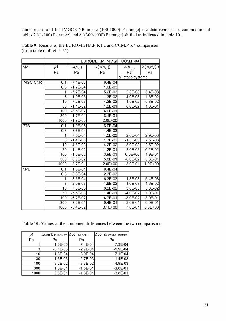
8. Link with CCM.P-K4 comparison The present results of the EUROMET.M.P-K1.a comparison can be linked to the results obtained in the CCM.P-K4 comparison /12/. Eight primary laboratories took part in the CCM.P-K4 comparison: four participants used static expansion systems and the other four used different types of column manometers in which the liquid levels were measured by laser or ultrasound interferometry. For the evaluation of the reference pressure values for EUROMET.M.P-K1a, the data from the five completely independent NMIs (IMGC-CNR, BNM-LNE, PTB, NPL, UME) have been considered three of which (IMGC-CNR, PTB, NPL) participated in both comparisons. IMGC-CNR participated in the CCM key comparison with two systems (static expansion system and interferometric manobarometer) while in the present comparison the static system was used for the full pressure range; so, for this laboratory, only the data in the (1-30) Pa range from the CCM comparison are considered in the linking procedure. The other two laboratories used the same system in both comparisons. In the present EUROMET comparison the calibrations were performed in the (0.1 – 1000) Pa pressure range while in the CCM.P-K4 comparison the range considered was from 1 Pa to 1000 Pa. To link the results of the two comparisons the common (1 - 1000) Pa range has been considered. Table 95shows a summary of the results for the three NMIs that participated in both the comparisons. As the transfer standards were not the same (even though they were based on the same principle) in the two comparisons, the reference values can be considered as not being related to the same quantity; consequently, a method of shifting one to the other must be applied. As suggested in /17/, the reference values of the EUROMET.M.P-K1a comparison should be shifted to the reference values of the CCM.P-K4 comparison. The size of the shift can be evaluated by considering the combined differences ∆combi /17/ of the three (or two) NMIs, calculated for each comparison, by the weighted mean of the respective differences ∆pi,j as follows:

( )( )

( )( )

( )( )

)(1

)(1

)(1

)()()(

,2

,2

,2

,2

,

,2

,

,2

,

PTBiNPLiIMGCi

PTBpi

PTBi

NPLi

NPLi

iMGCi

IMGCi

i

pUpUpU

pUp

pUp

pUp

comb

∆+

∆+

∆

∆∆

+∆

∆+

∆∆

=∆ [20]

So that it is possible to calculate the differences ∆combCCM and ∆combEUROMET for the CCM.P-K4 and EUROMET.M.P.-K1a comparisons respectively (table 10) and, consequently, the shift between the references values of EUROMET from CCM reference values as given by ∆combi,CCM –EUROMET

= ∆combi,CCM - ∆combi, EUROMET

Finally, the differences ∆pi,j of those NMIs that participated only in EUROMET comparison [and of IMGC-CNR for the (100-1000) Pa range] are shifted to the CCM reference values by using the combined differences ∆combi,CCM-EUROMET: ∆(pi,j)CCM = ∆(pi,j) + ∆combi,CCM-EUROMET For linking purposes, for the NMIs that participated in both comparisons data from CCM comparison are considered; for IMGC-CNR this only applies for the pressure interval (1-30) Pa. If the standards of the NMIs that participated in both comparison are stable it is suggested /17/ there should not be any additional uncertainty to consider when shifting the reference values. The linkage of the comparison results to CCM.P-K4 is summarized in table 11 (and in figure 1) in which the data for IMGC-CNR [(1-30)Pa range], PTB and NPL come from table 9 and originate from the CCM.P-K4 comparison and for the other NMIs that took part only in the EUROMET M.P-K1

21

comparison [and for IMGC-CNR in the (100-1000) Pa range] the data represent a combination of tables 7 [(1-100) Pa range] and 8 [(300-1000) Pa range] shifted as indicated in table 10. Table 9: Results of the EUROMETM.P-K1.a and CCM.P-K4 comparison (from table 6 of ref /12/ )

Table 10: Values of the combined differences between the two comparisons

EUROMET.M.P-K1.a CCM.P-K4NMI p t ∆(p i,j ) U (∆(p i,j )) ∆(p i,j ) U (∆(pi,j ) )

Pa Pa Pa Pa Paall static systems

IMGC-CNR 0.1 -7.4E-05 6.4E-040.3 -1.7E-04 1.6E-03

1 -7.7E-04 5.2E-03 2.3E-03 5.4E-033 -1.9E-03 1.3E-02 4.0E-03 1.6E-02

10 -7.2E-03 4.2E-02 1.5E-02 5.3E-0230 -1.1E-02 1.2E-01 6.0E-02 1.6E-01

100 -8.5E-02 4.0E-01300 -1.7E-01 6.1E-01

1000 -1.7E-03 2.0E+00PTB 0.1 1.9E-05 6.0E-04

0.3 3.6E-04 1.4E-031 7.5E-04 4.5E-03 2.0E-04 2.9E-033 -1.4E-03 1.3E-02 -1.3E-03 7.5E-03

10 -4.6E-03 4.2E-02 -5.0E-03 2.5E-0230 -1.4E-02 1.2E-01 2.0E-03 6.2E-02

100 -1.0E-02 3.9E-01 0.0E+00 1.9E-01300 8.9E-02 5.8E-01 -8.0E-02 5.6E-01

1000 3.7E-01 2.0E+00 -3.0E-01 1.9E+00NPL 0.1 1.5E-04 8.4E-04

0.3 3.8E-04 2.3E-031 8.5E-04 6.3E-03 1.3E-03 5.4E-033 2.0E-03 1.9E-02 1.0E-03 1.6E-02

10 7.8E-05 6.2E-02 3.0E-03 5.3E-0230 -5.5E-03 1.4E-01 -4.0E-02 1.0E-01

100 -6.2E-02 4.7E-01 -8.0E-02 3.0E-01300 3.2E-01 9.4E-01 -2.0E-01 9.0E-01

1000 -3.4E-02 3.1E+00 7.0E-01 3.0E+00

pt ∆comb EUROMET ∆comb CCM ∆comb CCM-EUROMET

Pa Pa Pa Pa1 1.6E-05 7.4E-04 7.3E-043 -8.1E-05 -2.7E-04 -1.9E-04

10 -1.8E-04 -8.9E-04 -7.1E-0430 -1.3E-03 -2.7E-03 -1.4E-03

100 -3.2E-02 -3.7E-02 -4.9E-03300 1.5E-01 -1.5E-01 -3.0E-01

1000 2.6E-01 -1.3E-01 -3.8E-01

22

Table 11: Comparison results as evaluated by ∆pi,j shifted for the NMIs participating only in the EUROMET.M.P-k1.a comparison and the expanded uncertainty from tables 7, 8 and 9.

NMI p t ∆p i,j U (∆p i,j) NMI p t ∆p i,j U (∆p i,j)

n.of NMI Pa Pa Pa n.of NMI Pa Pa PaIMGC-CNR 1 2.3E-03 5.4E-03 CEM 1 3.1E-03 9.0E-03

1 3 4.0E-03 1.6E-02 6 3 2.0E-03 2.4E-02 10 1.5E-02 5.3E-02 10 -7.2E-03 7.9E-02

30 6.0E-02 1.6E-01 30 -3.7E-02 2.0E-01100 -8.0E-02 4.0E-01 100 -1.5E-01 6.3E-01300 1.3E-01 6.1E-01 300 -3.0E-01 1.3E+00

1000 3.8E-01 2.0E+00 1000 -3.8E-01 4.2E+00BNM.LNE 1 -5.6E-03 5.1E-03 NPL 1 1.3E-03 5.4E-03

2 3 -1.7E-02 1.3E-02 7 3 1.0E-03 1.6E-0210 -4.0E-02 4.1E-02 10 3.0E-03 5.3E-0230 -7.8E-02 1.1E-01 30 -4.0E-02 1.0E-01

100 -1.7E-01 3.8E-01 100 -8.0E-02 3.0E-01300 -3.0E-01 5.7E-01 300 -2.0E-01 9.0E-01

1000 -3.8E-01 1.9E+00 1000 7.0E-01 3.0E+00MIKES 1 3.9E-02 4.4E-02 OMH 1 8.2E-04 8.2E-02

3 3 4.1E-02 5.2E-02 8 3 -9.3E-02 2.3E-0110 4.3E-02 8.2E-02 10 -4.0E-01 9.2E-0130 5.0E-02 2.0E-01 30 2.0E+00 3.2E+00

100 7.7E-02 7.0E-01 100 2.5E+00 3.1E+00300 -1.0E-01 1.3E+00 UME 1 6.2E-03 6.0E-03

1000 3.2E-01 4.5E+00 9 3 1.8E-02 1.8E-02SP 1 2.8E-03 3.8E-02 10 5.1E-02 5.8E-02

4 3 5.6E-03 6.8E-02 30 1.1E-01 1.4E-0110 -8.0E-03 1.3E-01 100 3.2E-01 4.7E-0130 -5.5E-02 3.2E-01 NMi 1 3.6E-03 3.5E-02

100 -1.5E-01 9.6E-01 10 3 -3.3E-02 3.6E-02300 -3.0E-01 1.3E+00 10 5.8E-03 3.7E-02

1000 5.1E-01 2.3E+00 30 6.4E-02 4.2E-02PTB 1 2.0E-04 2.9E-03 100 9.6E-02 6.9E-02

5 3 -1.3E-03 7.5E-0310 -5.0E-03 2.5E-0230 2.0E-03 6.2E-02

100 0.0E+00 1.9E-01300 -8.0E-02 5.6E-01

1000 -3.0E-01 1.9E+00

23

Figure 1 a: Comparison results: the differences ∆pi,j with their expanded uncertainty, for each participating NMI at the pressure level from 1 Pa to 30 Pa.

1Pa

-1E-01

-8E-02

-6E-02

-4E-02

-2E-02

0E+00

2E-02

4E-02

6E-02

8E-02

1E-01

0 1 2 3 4 5 6 7 8 9 10 11

∆pij

3 Pa

-4.0E-01

-3.0E-01

-2.0E-01

-1.0E-01

0.0E+00

1.0E-01

2.0E-01

0 1 2 3 4 5 6 7 8 9 10 11

∆pij

10 Pa

-2E+00

-1E+00

-5E-01

0E+00

5E-01

1E+00

0 1 2 3 4 5 6 7 8 9 10 11

∆pij

30 Pa

-2E+00

-1E+00

0E+00

1E+00

2E+00

3E+00

4E+00

5E+00

6E+00

0 1 2 3 4 5 6 7 8 9 10 11

∆pij

24

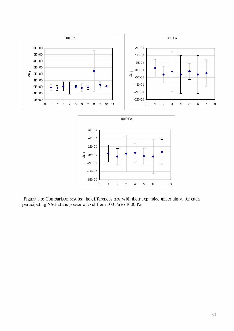
Figure 1 b: Comparison results: the differences ∆pi,j with their expanded uncertainty, for each participating NMI at the pressure level from 100 Pa to 1000 Pa

100 Pa

-2E+00

-1E+00

0E+00

1E+00

2E+00

3E+00

4E+00

5E+00

6E+00

0 1 2 3 4 5 6 7 8 9 10 11

∆pij

300 Pa

-2E+00

-2E+00

-1E+00

-5E-01

0E+00

5E-01

1E+00

2E+00

0 1 2 3 4 5 6 7 8

∆pij

1000 Pa

-6E+00

-4E+00

-2E+00

0E+00

2E+00

4E+00

6E+00

0 1 2 3 4 5 6 7 8

∆pij

25

9. References /1/ Bergoglio M., Calcatelli A., Vacuum measurement and traceability in Italy, Proc. XIV IMEKO World Congress, Tampere, June 1997 /2/ Legras J.C., Le Guinio J. and Baron F., Calibration chain of BNM-LNE from 10-4 Pa to 10 kPa, Metrologia, 36, 1999, 631-635 /3/ Takaishi T., Sensui Y., Thermal transipiration effect of hydrogen, rare gases and methane, Trans. Faraday Soc., 1963, 59,2503-2514 /4/ Jitschin W., Migwi J.K., Grosse G., Pressures in the high and medium vacuum range generated by a series expansion standard, Vacuum, 1990, 40, 293-304 /5/ Jousten K., Rohl P., Contreras V. A., Volume ratio determination in the static expansion system by means of a spinning rotor gauge, Vacuum, 1999, 52, 491-499 /6/ Elliott K. W. T., Clapham P. B., The accurate measurement of the volume ratios in vacuum vessel, NPL Report MOM 28, January 1978 /7/ Redgrave F. J., Forbes A. B., Harris P. M., A discussion of methods for estimation of volumetric ratios determination by multiple expansion, Vacuum, 1999, 53, 159-162 /8/ Sommer K. D. and J. Poziemski, Expansion and Compressibility of Mercury, Metrologia 30, 1993/94, 665-668 /9/ Bergoglio M., Calcatelli A, Some considerations on handling the calibration results of capacitance membrane gauges, Vacuum, 60, 2001, 153,159 /10/ Bergoglio M.,Considerations on fitting models applied to capacitance membrane diaphragms, IMGC-CNR Technical report n. 92, January 2003 /11/ Miiller A.P., Measurement performance of high-accuracy low-pressure transducers, Metrologia, 36, 1999, 617-621 /12/ Miiller A. P. et al, Final report on key comparison CCM.P-K4 of absolute pressure from 1 Pa to 1000 Pa, Metrologia Suppl. 07001, 2002 and final report available on web BIPM database, (http:kcdb.www.bipm.org) /13/ Kacker R. and Jones A., On use of Bayesian statistics to make the Guide to the expression of the uncertainty in measurement consistent, Metrologia,40,2003, 235-248 /14/ Guideline for CIPM comparison, Appendix F to MRA, March 1999 , (http:www.bipm.org) /15/ Cox M. G., The evaluation of key comparison data, Metrologia, 39, 2002, 589-595 /16/ Guide to expression of uncertainty in measurement, BIPM-ISO, 1993, ISBN 92-96-10088-9 /17/ Legras, J.C., How to link regional comparisons to a CIPM key comparison, document presented at the meeting of the group chairmen held in Dubrovnik in June 2003

FINAL REPORT Key comparison...

Documents

Transcript of FINAL REPORT Key comparison...