1

Final Report Aerial thermal imaging applied to Wisconsin’s groundwater,

springs, thin soils, and slopes.

Principal Investigator: David J. Hart, Wisconsin Geological and Natural History Survey Co-Investigator: Susan K. Swanson, Beloit College

Co-Investigator: J. Elmo Rawling III, Wisconsin Geological and Natural History Survey

DATCP 2020-3

2

TABLE OF CONTENTS

LIST OF FIGURES AND TABLES ............................................................................................................. 3

PROJECT SUMMARY ................................................................................................................................ 4

INTRODUCTION ........................................................................................................................................ 6

PROCEDURES AND METHODS ............................................................................................................... 6

RESULTS AND DISCUSSION ................................................................................................................... 8

CONCLUSIONS AND RECOMMENDATIONS ..................................................................................... 13

REFERENCES ........................................................................................................................................... 14

APPENDIX A: ............................................................................................................................................ 16

APPENDIX B: ............................................................................................................................................ 17

3

LIST OF FIGURES AND TABLES

Figure 1. Locations of the study sites in Wisconsin.

Figure 2. sUAS aerial photograph of the field showing locations of exposed bedrock and sinkholes, push probe depths, EM31 ground conductivity, and soil temperatures from the UAV infrared camera.

Figure 3. Best fit line and R2 values for the EM 31 and push probe data and for the UAV soil temperatures and the push probe data.

Figure 4. Temperature propagation depth with time using the soil temperature measurements.

Figure 5. Paired aerial optical and thermal images for limocrenes in Dane County (A. and B.) and Waukesha County (C. and D.).

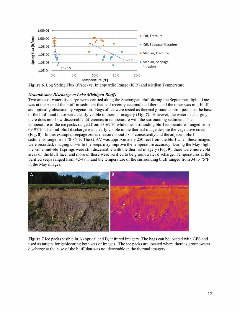
Figure 6. Log Spring Flux (ft/sec) vs. Interquartile Range (IQR) and Median Temperature.

Figure 7 Ice packs visible in A) optical and B) infrared imagery.

Figure 8. Thermal image overlaid on optical image showing discrete areas of groundwater discharge.

Figure 9. Thermal image of bluff in May.

Table 1. Dimensional analysis of thermal propagation depths with time.

4

PROJECT SUMMARY

Title: Aerial thermal imaging applied to Wisconsin’s groundwater, springs, thin soils, and slopes.

Project I.D.: DATCP2020-3

Investigators: David J. Hart, Professor, Wisconsin Geological and Natural History Survey, UW-Madison; J. Elmo Rawling III, Professor, Wisconsin Geological and Natural History Survey, UW-Madison; Susan K. Swanson, Professor of Geology, Beloit College

Period of Contract: July 1, 2019 - June 30, 2020

Objectives: Apply aerial thermal imaging to three groundwater issues in Wisconsin using a small unmanned aerial vehicle (sUAV) and a thermal camera. These include: 1) Determine depth to shallow bedrock over the Silurian dolomite in eastern Wisconsin at the field scale quickly, accurately and cost effectively, 2) Locate springs discharging to lakes and characterize temperature conditions in springs discharging to streams, and 3) Identify areas on Lake Michigan bluffs where groundwater discharge might lead to slope failure.

Methods: A FLIR Vue Pro R thermal camera collected thermal images (model 336x256, 25°x19° for shallow bedrock and bluffs and model 640x 45°x35° for limnocrene and rheocrene springs). For aerial applications, the thermal camera was mounted to a DJI Phantom 4 Advanced sUAV using a sUAS gimble. Both optical and thermal images were collected simultaneously, though controlled separately, and correlated afterward based on their timestamps. Camera radiometry settings were set in the field for surface emissivity, air temperature, cloud cover, humidity, and shooting distance, with the FLIR UAV mobile app. FLIR Tools + and ArcMap software aided processing of thermal images.

Results and Discussion: The sUAV mounted thermal camera soil temperatures showed some correlation to depth to bedrock. Shallow bedrock was warmer and deeper bedrock was cooler. Bedrock fractures were also identified in the soil temperatures. The resulting image covered much of the field and was collected in about an hour.

The sUAV mounted thermal camera did not detect substantial temperature differences due to the existence of limnocrenes because colder, denser spring water was not present at the water surface. The spatial distribution of water surface temperature within 1 meter of rheocrenes is more consistent and the median temperature tends to be colder for fracture springs than for seepage-filtration springs.

The sUAV mounted thermal camera detected temperature differences where groundwater discharges mid-bluff. The sUAV

5

mounted thermal camera did not detect temperature where water seeps from the base of the bluff.

Conclusions/Implications/ Recommendations: Although the soil temperature measurements alone will not

accurately predict bedrock depth, they do provide a screening tool that can guide other measurements that together can provide accurate bedrock depths. The sUAV mounted thermal camera will likely have other uses for agriculture such as irrigation scheduling and determining best planting times. The camera, gimbal, and sUAV used in this study are readily available at a cost of less than $10,000.

The sUAV mounted optical camera may be a simpler and more effective way to identify limoncrenes where the springs displace organic matter and as long as water clarity is high. This work shows that the ground based thermal camera can be used to characterize temperature conditions in rheocrenes. Inverse relationships between log spring flux and water temperature summary statistics suggest that spring flux, which is more easily measured, may also be a useful predictor of the spatial distribution of temperature in fracture and seepage filtration springs in Wisconsin.

The sUAV mounted camera is a relatively inexpensive option to further investigate how spatial and temporal variation of groundwater discharge influence bluff failure in the Great Lakes.

Related Publications: N/A

Key Words: unmanned aerial vehicles, thermal imaging, Silurian bedrock, depth to bedrock, springs, Lake Michigan, bluffs

Funding: Wisconsin Department of Agriculture, Trade and Consumer Protection (DATCP) and the University of Wisconsin Water Resources Institute (WRI) (WR19R003)

6

INTRODUCTION

In recent years, thermal imaging and small unmanned aerial vehicle (sUAV) technology has matured, become more accessible, and has been applied to hydrogeologic problems including stream/groundwater interactions (Briggs and others, 2014; Loheide and Gorelick, 2006), seepage faces (Deitchman and Loheide, 2009), and coastal discharge (Lee and others, 2016). Given the general usefulness of heat as a groundwater tracer (Anderson, 2005), development of more applications and instrumentation is likely. This project tested thermal imagery for three ground and surface water management issues of concern across Wisconsin (Fig. 1). These include: 1) Determine depth to shallow bedrock over the Silurian dolomite in eastern Wisconsin at the field scale quickly, accurately and cost effectively, 2) Locate springs discharging to lakes and characterize temperature conditions in springs discharging to streams, and 3) Identify areas on Lake Michigan bluffs where groundwater discharge might lead to slope failure.

Recent changes to the Wisconsin Department the Natural Resource’s (WNDR) rules governing land spreading of manure (Wisconsin Administrative Code Chapter NR151 Runoff Management) have increased the need for accurate, high resolution, low cost estimations of the depth to bedrock. The rules restrict spreading of manure on any fields where the depth to bedrock is less than 2 feet, and application

rates are restricted where the depth to bedrock is between 2 and 3 feet, in areas where the Silurian dolomite is the uppermost bedrock.

Wisconsin’s statewide inventory of springs characterized 415 large (0.25 cfs or more) springs (Swanson and others, 2019). While the inventory was successful in locating rheocrenes (springs discharging to streams), it was less successful in locating limnocrenes (springs discharging to lakes), due to their lack of visibility from the shoreline. Yet limnocrenes with discharges of 1ft3/sec or more are important in Wisconsin because they may still meet the

requirements for evaluation of significance of impacts under the groundwater withdrawals section of the Wisconsin Statutes (Wis. Stat. § 281.34). Thermal imaging also holds potential for characterizing the spatial distribution of temperatures in springs. Cold and stable temperatures are often cited as important ecological conditions in springs (Gaffield and others, 2005; Knight and Notestein, 2008), but there is currently a lack of information on the spatial distribution of temperatures in springs and how distributions vary among springs of differing types.

High lake levels (Smith and others, 2016) are reducing beach area along the Lake Michigan coastline and allowing wave action to erode the bases of coastal bluffs at the highest rate of the past 30 years. Water table elevation and perched flow systems associated with seepage faces are dominant factors in bluff stability. Mapping of the distribution of seepage faces along the bluffs also informs our understanding of the hydrogeology of the sediments that form the bluffs, allowing a two-dimensional view of these layered sediments

PROCEDURES AND METHODS

A FLIR Vue Pro R thermal camera collected thermal images (model 336x256, 25°x19° for shallow bedrock and bluffs and model 640x 45°x35° for limnocrene and rheocrene springs). For aerial

Figure 1. Locations of the study sites in Wisconsin.

7

applications, the thermal camera was mounted to a DJI Phantom 4 Advanced sUAV using a sUAS gimble. Both optical and thermal images were collected simultaneously, though controlled separately, and correlated afterward based on their timestamps. Camera radiometry settings were set in the field for surface emissivity, air temperature, cloud cover, humidity, and shooting distance, with the FLIR UAV mobile app. FLIR Tools + and ArcMap software aided processing of thermal images.

The camera shooting distance, field of view, and pixel resolution were important considerations for flight planning and image processing. The shooting distance, or altitude, of the thermal camera influences the spatial coverage and resolution of the images. Flights were conducted from different altitudes for the three aerial applications. The shallow bedrock and bluff sites both involved creating thermal mosaics from multiple images. At these sites, a longer shooting distance increased the ability to cover areas efficiently. When constructing thermal mosaics, automating the flight improved altitude control, which in turn resulted in a more consistent field of view and pixel size. Thus, automating the flight improved the clarity and spatial accuracy of the image merging. We programmed the sUAS to hover and collect images at positions spaced along a grid to produce 35-40% image overlap. Flight paths were created in ArcMap and imported to an autopilot mobile app (DJI GS Pro) for flight configuration. Thermal images were collected on a 1-3 second time interval, which was at least half the length of the aircraft hover time, to ensure a choice of thermal images from each location for the mosaics.

Depth to Bedrock Flights for the depth to bedrock study were conducted over an agricultural field in Kewaunee County with shallow Silurian bedrock (Fig. 1). Depths to bedrock in the field range from 0 ft where it outcrops to more than 3ft (0.9 m) based on soil probe data. Aerial thermal images were collected from altitudes of 250-300 ft (76-91 m) in November and March, after harvest and before spring planting, using the methods described above. Push probe measurements and geophysical surveys (EM-31, Dual EM, Electrical resisitivity) were also collected in overlapping areas for comparison. Thermal mosaics generated with FLIR Tools + were converted to rasters and imported to ArcMap for statistical analysis. The rasters were georeferenced based on the positions of ice packs, people, vehicles, and other thermal/visual targets located in the field with GPS. We attempted to collect thermal images at a second field but encountered winds greater than 10 miles per hour that caused the drone to crash.

Soil and air temperature measurements with depth were also collected at two locations at the agricultural field. This was done to provide an understanding of how quickly temperature variations propagate through the soils. Seven DS18b20 temperature sensors and an Arduino data logging system measured temperatures just above the ground surface and at six depths down to the bedrock surface at a depth of 1.3 feet at the first location and to a depth of 3 ft without contacting bedrock at the second location. These data were recorded at 5-minute intervals from November 21st to December 1st.

Groundwater Discharge to Surface Waters The two springs selected for evaluation of the ability to discriminate limnocrenes from the lakes to which they discharge are near the headwaters of the Mukwanago River and along Nine Springs Creek in Waukesha and Dane Counties, respectively (Fig. 1). The springs have seepage/filtration morphologies with boiling sands extending at least two meters from one or more central orifices. They have discharge rates of 1ft3/sec or more, and the water depth at both sites is approximately 3.3 feet (1 m) (Swanson et al., 2019). The sUAV mounted thermal and optical cameras took multiple paired images from heights of approximately 30 to 50 feet (9 to 15 m) above the water surface using the procedures described above. The flights were conducted on June 16 and 18, 2020.

Ten fracture springs and ten seepage-filtration springs comprise the twenty rheocrenes selected to characterize the spatial distribution of spring surface temperatures and to evaluate how the distributions vary among springs of differing types (Fig. 1). Measured water depths at the time of data collection

8

ranged from 3 to 44 cm, with an average of 20 cm. A range pole, tripod, and overhead camera boom positioned the thermal camera 90° from and 4 feet (1.2 m) above the water surface. Because the FLIR Vue Pro 640 camera has a 45° FOV, this results in a lateral distance across the bottom of the thermal images of about 1 m. Water depth was measured within the imaged area at each spring. The images are composed of 640 x 512 pixels, so the effective pixel size of each image is 2.4 mm2. A 60 ft2 (6.6 m2) umbrella shaded the spring pool to minimize reflected radiation from clouds and tree canopy. The FLIR UAS app (version 2.2.4) recorded field measurements of air temperature, distance to water surface, humidity, and cloud cover at the time of data collection. Emissivity was set at 0.98 because fresh water approximates a black body (Torgersen et al., 2001). At least four thermal images were captured within 1 m of a spring orifice at each site in June 2020. A digital camera captured optical images at the same position and height as the thermal camera. Spring flow, for use in spring flux calculations, was measured using a wading rod and acoustic Doppler velocity meter or an 8-inch cutthroat flume. Spring area was measured in the field or estimated from existing site maps (Swanson et al., 2019).

Temperature arrays were extracted from the thermal images using the FLIR Tools+ software and then imported to ArcMap (version 10.7.1, ESRI), where optical images could be displayed and georeferenced to thermal rasters. Prior to summarizing the spatial distribution of water surface temperatures, all images were corrected by performing off-axis vignetting compensation using the process described by Pour et al. (2019). If necessary, images were clipped to avoid terrestrial objects or areas of high reflectivity due to rough water surfaces. Histograms of number of pixels and summary statistics (median, interquartile range) provide information on the distribution of surface temperature near each spring orifice.

Groundwater Discharge to Lake Michigan Bluffs Flights over Lake Michigan bluffs were conducted in September and May, when air temperatures were 60°F and 70°F (21°C), respectively. The site selected for the study, located north of Sheboygan, Wisconsin (Fig. 1), had areas of groundwater seepage known from previous work (Krueger et al., in review; Rolland et al., in review; Volpano et al., 2020). In September 2019, oblique images were collected along the length of the bluff property. Seepage areas suggested from this preliminary imaging were visually confirmed by walking the shore and they were geolocated with GPS. The site was returned to in May 2020 for automated flights designed using the methods described above. An automated flight collected oblique images from 250 feet distance parallel to the shoreline. This distance ensured the full height of the bluff fit in the camera’s vertical field of view. Automated flights were also programmed to collect nadir images from 150, 200, and 250 feet altitudes over the identified groundwater seeps. Representative images were selected from each flight and merged together using the FLIR Tools + Panorama tool.

RESULTS AND DISCUSSION

Depth to Bedrock We sought to use a UAV mounted infrared camera to identify areas of shallow bedrock in agricultural fields. If successful, this would allow farmers and their consultants to quickly map their fields and more readily comply with land spreading regulations, Wisconsin’s NR151 runoff management code. Many agricultural consultants own and operate UAVs and so have the expertise to apply this method.

We compared the UAV infrared temperatures and geophysical measurements with depths to bedrock measured from hand push probes. An aerial photograph of the field showing locations of exposed bedrock and sinkholes, push probe depths, EM31 ground conductivity, and soil temperatures from the UAV infrared camera are shown in Figure 2. The depths to bedrock are most shallow at the west and east. In those areas the push probe depth to bedrock is less than 24 inches as shown by the red and yellow circles and squares and the numerous bedrock exposures. The EM 31 ground conductivity is lowest in these same regions shown as the red and yellow dots along the EM 31 survey lines. The soil temperatures

9

are highest in these areas of shallow bedrock as shown by the reddish shading. The areas of deeper bedrock in the push probe data in the middle of the image correspond to higher ground conductivities (green and blue along the EM 31survey line) and lower soil temperatures (green and yellow shading). The UAV soil temperatures also showed bedrock fractures. Figure 2 shows fractures in the field to the west of the study field. The fractures can be seen in the air photo continuing on the other side of the road as cooler yellow lines inset in the warmer reddish unfractured bedrock.

Figure 2. sUAS aerial photograph of the field showing locations of exposed bedrock and sinkholes, push probe depths, EM31 ground conductivity, and soil temperatures from the UAV infrared camera. Note fractures evident in vegetation to the west of the study field and as cooler yellow lines in thermal image.

A more quantitative analysis of correlations between the EM 31, UAV soil temperatures and the push probe depths was conducted. We used ArcGIS to select the nearest EM 31 and UAV soil temperatures the push probe data points located nearest and less than 20 feet from the push probe data points. These data pairs were plotted and a linear regression analysis was conducted. Figures 3a and 3b show the best fit line and R2 values for the EM 31 and push probe data and for the UAV soil temperatures and the push probe data. While there are definite observable trends in the data, the R2 values are low. This means that neither the EM 31 or the soil temperature should be used alone to predict actual depths. It is more appropriate to use them in conjunction with push probe data and to establish ranges rather than exact values of bedrock depth.

This method depends on shallow bedrock with thin soils providing a different temperature signature than deeper bedrock with thick soils. A dimensional analysis of propagation depth using a representative thermal diffusivity (α=1x10-6 m2/s) and time is provided in Table 1. This analysis suggests that propagation times longer than one day are needed for this method to be successful.

10

Figure 3. Best fit line and R2 values for the EM 31 and push probe data and for the UAV soil temperatures and the push probe data.

Table 1. Dimensional analysis of thermal propagation depths with time.

Time (days | seconds) Propagation Depth (m | ft)

0.5 days | 43,200 seconds 0.21 m | 0.7 ft

2.0 days | 172,800 seconds 0.41 m | 1.4 ft

11.6 days | 1,000,000 seconds 1.00 m | 3.3 ft

𝑑𝑑𝑑𝑑𝑑𝑑𝑑𝑑ℎ = �𝑑𝑑𝑡𝑡𝑡𝑡𝑑𝑑 × 𝑑𝑑ℎ𝑑𝑑𝑒𝑒𝑡𝑡𝑒𝑒𝑒𝑒 𝑑𝑑𝑡𝑡𝑑𝑑𝑑𝑑𝑑𝑑𝑑𝑑𝑡𝑡𝑑𝑑𝑡𝑡𝑑𝑑𝑑𝑑

We checked the temperature propagation depth with time using the soil temperature measurements. These measurements are plotted in Figure 4. From that plot, the coldest air temperature was observed in the very early morning of November 23rd. The shallowest buried sensor T2 records its coldest temperature several hours later and the deepest sensor T7 located across depths of 1.04 -1.33 feet records its lowest temperature more than 24 hours later. The rapid daily temperature swings seen in the air temperature sensor are attenuated and delayed with greater depths and are not observed in the deepest sensor.

Groundwater Discharge to Surface Waters The thermal images of the surface waters to which the limnocrenes discharge do not show discernable differences in temperature in the vicinity of the springs (Fig. 5). Although the water surface temperature above the Nine Springs limnocrene is slightly cooler, visible contrasts in temperature are due mostly to adjacent vegetation or floating organic matter. Because the thermal camera detects thermal radiation

Figure 4. Temperature propagation depth with time using the soil temperature measurements.

11

emitted from the upper 0.1 mm of the water surface and the images were captured in late June when surface water temperatures are higher than groundwater temperatures, it is likely that cooler and denser groundwater remained below the water surface, preventing detection of the limnocrenes with airborne thermal imaging (Torgersen et al., 2001; Hare et al., 2015). However, the sandy substrate in the vicinity of the limnocrenes is clearly visible in the optical images. Therefore, as long as the discharge is high enough to displace organic matter on the lake bed and water clarity is high, optical images alone are likely to be sufficient to identify and map limnocrenes that are otherwise inaccessible.

Figure 5. Paired aerial optical and thermal images for limocrenes in Dane County (A. and B.) and Waukesha County (C. and D.). Sandy spring boils in A. and C. are 2-4 meters in diameter.

The ground-based thermal images and associated histograms show that few of the temperature distributions exhibit normality. As a result, the interquartile range (IQR) and median temperature are used as measures of spread and central tendency (Appendix B). The spatial distribution of water surface temperature within 1 meter of a spring orifice is more consistent for fracture springs than for seepage-filtration springs. The interquartile ranges (IQR) for fracture springs range from 0.18 to 0.49℃, whereas the IQRs for seepage-filtration springs range from 0.51 to 1.50℃. Fracture springs also generally have colder surface water temperatures within 1 meter of the spring orifice. Median temperatures for the fracture springs range from 8.56 to 12.01℃, except for DN6FR (14.47℃). DN6SP, a seepage-filtration spring at the same site, has a very similar median temperature (14.39℃). Median water surface temperatures for the seepage-filtration springs range from 11.87 to 16.38℃, except for WK2 (10.35℃). Overall, the seepage-filtration springs exhibit more complex distributions; eight of the seepage-filtration springs, as opposed to just two of the fracture springs, exhibit two or three density peaks.

Spring flux (ft/sec), defined as spring flow (ft3/sec) divided by the area of discharge (ft2), is thought to provide a meaningful way to distinguish between features dominated by discrete versus diffuse groundwater flow, with higher spring flux values being representative of more discrete discharge (Swanson et al., 2019). For the springs investigated in this work, spring flux ranges from 4.8E-04 to 2.2E-02 ft/sec for the seepage-filtration springs and 2.3E-02 to 1.4E+00 ft/sec for the fracture springs (Appendix B). A goal of this study was to determine if relationships exist between spring flux and temperature summary statistics, which would allow the use of spring flux as a predictor of the spatial distribution of water surface temperature in springs of differing types. Figure 6 shows a moderate inverse relationship between log spring flux and IQR (R2 = 0.5) and a weak inverse relationship between log spring flux and median surface water temperature (R2 = 0.3).

12

Figure 6. Log Spring Flux (ft/sec) vs. Interquartile Range (IQR) and Median Temperature.

Groundwater Discharge to Lake Michigan Bluffs Two areas of water discharge were verified along the Sheboygan bluff during the September flight. One was at the base of the bluff in sediment that had recently accumulated there, and the other was mid-bluff and optically obscured by vegetation. Bags of ice were tested as thermal ground control points at the base of the bluff, and these were clearly visible in thermal imagery (Fig. 7). However, the water discharging there does not show discernable differences in temperature with the surrounding sediment. The temperature of the ice packs ranged from 53-69°F, while the surrounding bluff temperatures ranged from 69-97°F. The mid-bluff discharge was clearly visible in the thermal image despite the vegetative cover (Fig. 8). In this example, seepage zones measure about 58°F consistently and the adjacent bluff sediments range from 70-85°F. The sUAV was approximately 250 feet from the bluff when these images were recorded; imaging closer to the seeps may improve the temperature accuracy. During the May flight the same mid-bluff springs were still discernable with the thermal imagery (Fig. 9), there were more cold areas on the bluff face, and more of these were verified to be groundwater discharge. Temperatures at the verified seeps ranged from 42-48°F and the temperature of the surrounding bluff ranged from 34 to 75°F in the May images.

Figure 7 Ice packs visible in A) optical and B) infrared imagery. The bags can be located with GPS and used as targets for geolocating both sets of images. The ice packs are located where there is groundwater discharge at the base of the bluff that was not detectable in the thermal imagery.

13

Figure 8. Thermal image overlaid on optical image showing discrete areas of groundwater discharge. These seeps (shown as dark blue) are 12-23°F colder than the surrounding bluffs but were not visible in the optical imagery due to obscuration by vegetation.

Figure 9. Thermal image of bluff in May: A = dead vegetation, B = Lake Michigan, C = stream discharging from gully, D = bluff crest, E = conifer vegetation, F = sUAS pilot. Mid-bluff groundwater discharge is shown with circles, many of these were not active during an April visit when the weather prevented a flight.

CONCLUSIONS AND RECOMMENDATIONS

Depth to Bedrock Soil surface temperatures measured by the sUAV mounted thermal camera appear correlated with shallow bedrock depths measured with a hand probe. The correlation between the soil surface temperature and bedrock depth was similar to ground conductivity measurements from an EM31 and bedrock depth. However, the degrees of correlation is not sufficient for soil surface temperatures or the EM31 alone to provide accurate bedrock depths. These measurements require additional data to provide more reliable depth to bedrock estimates. Hand probes or additional frequency and coil orientation ground conductivity measurements would provide that data. The cost of the sUAV thermal mounted camera and gimbal was less than $5000, making it a less expensive option than ground conductivity meters such as the EM31. Soil surface temperatures might also be used to guide other agricultural decisions such as irrigation schedules or planting. One unknown is the importance of antecedent temperatures. It may be that large temperature changes are needed a week prior to the measurements so that the temperatures can propagate to the depths of interest.

14

Groundwater Discharge to Surface Waters The sUAV mounted thermal camera did not detect substantial temperature differences due to the existence of limnocrenes. Because the thermal camera only detects radiation emitted from the upper water surface and the water depth is at least 1 m at both sites, it is likely that groundwater does not reach the surface of the water body at either site. This condition is more likely during summer months when groundwater is often colder and denser than surface water. As a result, remote thermal imaging is unlikely to be an effective way to locate limnocrenes in Wisconsin, even in late fall or winter when temperature and density conditions are reversed, because hunting and inclement winter weather may limit opportunities to fly a sUAV. Instead, the sUAV mounted optical camera may be a simpler and more effective way to identify limoncrenes where the springs displace organic matter and as long as water clarity is high.

The spatial distribution of water surface temperature within 1 meter of springs discharging to streams is more consistent and the median temperature tends to be colder for fracture springs than for seepage-filtration springs. These results align with observations of focused groundwater discharge from exposed fractures versus heterogeneous, distributed discharge from seepage-filtration springs and suggest that orifice geometry can influence the spatial distribution of surface water temperature in springs. Because shallow water depths and high water velocities near the spring orifices likely promoted mixing, surface distributions may also be representative of temperature distributions within the water column. While this work shows that the ground based thermal camera can be used to characterize temperature conditions in rheocrenes, inverse relationships between log spring flux and water temperature summary statistics suggest that spring flux, which is more easily measured, may also be a useful predictor of the spatial distribution of temperature in fracture and seepage filtration springs in Wisconsin.

Groundwater Discharge to Lake Michigan Bluffs The sUAV mounted thermal camera detected spring discharge along the study reach of Lake Michigan bluffs in the spring and fall. Groundwater discharging from mid-bluff seeps are clearly discernible in the thermal imagery (Fig. 10), even in areas of light vegetation that obscures the optical images. However, other vegetated and shaded areas of the bluff are also “cold” and therefore the thermal imagery should be used to target areas for field verification. Any areas of water discharge are weaker and more susceptible to erosion, however, not all of these are detectible with thermal imagery. For example, water percolating through colluvium at the base of the bluff is likely able to come into thermal equilibrium with sediment and was not detectable with the thermal camera. More springs were detected in May, likely due to increased seasonal precipitation and snowmelt. Finally, a seasonal increase in discharge in May is consistent with Volpano et al., (2020) and Rolland et al., (in review) observation of more erosion then, contrary to previous studies that suggested large summer storms dominated seasonal erosion (Castedo et al., 2013). These observations demonstrate the feasibility of mounting a relatively inexpensive thermal camera to a common sUAS platform to further investigate how spatial and temporal variation of groundwater discharge influence bluff failure in the Great Lakes.

REFERENCES

Anderson, M.P. (2005) Heat as a Groundwater Tracer. Groundwater, Vol. 43, 951-968. http://dx.doi.org/10.1111/j.1745-6584.2005.00052.x

Briggs, M.A., Lautz, L.K., Buckley, S.F., Lane, J.W. (2014) Practical limitations on the use of diurnal temperature signals to quantify groundwater upwelling: Journal of Hydrology, vol. 519, pp. 1739-1751. http://dx.doi.org/10.1016/j.jhydrol.2014.09.03

Castedo, R., Fernández, M., Trenhaile, A.S., and Paredes, C. (2013). Modeling cyclic recession of cohesive clay coasts: Effects of wave erosion and bluff stability. Marine Geology, 335, p. 162–176. https://doi.org/10.1016/j.margeo.2012.11.001.3

15

Deitchman, R.S., and Loheide II, S.P. (2009) Ground-based thermal imaging of groundwater flow processes at the seepage face, Geophysical Research Letters, Vol. 36, doi: 10.1029/2009GL038103.

Gaffield, S.J., Potter, K.W., and Wang, L. (2005) Predicting the summer temperature of small streams in southwestern Wisconsin: Journal of the American Water Resources Union, Vol. 41, doi: 10.1111/j.1752-1688.2005.tb03714.x.

Hare, D.K., Briggs, M.A., Rosenberry, D.O., Boutt, D.F., Lane, J.W., 2015, A comparison of thermal infrared to fiber-optic distributed temperature sensing for evaluation of groundwater discharge to surface water: Journal of Hydrology 530: 153-166.

Knight, R.L., Notestein, S.K. (2008) Springs as Ecosystems, in Summary and Synthesis of the Available Literature on the Effects of Nutrients on Spring Organisms and Systems: University of Florida Water Institute, p.1-46.

Krueger, R., Zoet L.K., and Rawling III, J.E., (in review) Coastal bluff evolution in response to a rapid rise in surface water level, Journal of Geophysical Research-Earth Surface.

Lee, E., Kang, K., Hyun, S., Lee, K., Yoon, H., Kim, S., Kim, ., Xu,Z., Kim, D., Koh, D., and Ha, K. (2016) Submarine groundwater discharge revealed by aerial thermal infrared imagery: a case study on Jeju Island, Korea. Hydrological Processes Vol. 30, No. 19, https://doi.org/10.1002/hyp.10868

Loheide, S.P., II and Gorelick, S.M. (2006) Quantifying stream-aquifer interactions through analysis of remotely sensed thermographic profiles and in-situ temperature histories: Environmental Science and Technology, Vol. 40, No. 10, p. 3336–3341.

Pour, T., Mirijovsky, J., Purket, T., 2019, Airborne thermal remote sensing: the case of the city of Olomouc, Czech Republic. European Journal of Remote Sensing 52 (S1): 209-218.

Rolland, C., Zoet, L.K, Rawling III, J.E., and Cardiff, M., (in review) Seasonality in cold coast bluff erosion processes, Quaternary Research.

Smith, J.P., Hunter,T.S., Clites, A.H., Stow, C.A., Slawecki, T., Muhr, G.C. & Gronwold, A.D., (2016). An expandable web-based platform for visually analyzing basin-scale hydro-climate time series data. Environmental Modelling & Software 78, 97-105.

Swanson, S. K., Graham, G. E., and Hart, D. J., 2019, An Inventory of Springs in Wisconsin: Wisconsin Geological and Natural History Survey Bulletin 113, 24 p.

Torgersen, C.E., Faux, R.N., McIntosh, B.A., Poage, N.J., Norton, D.J., 2001, Airborne thermal remote sensing for water temperature assessment in rivers and streams. Remote Sensing of Environment 76: 386–398.

Volpano, C, Zoet, L.K. Rawling III, J.E, and Thauerkauff, E. (2020). Three-Dimensional Bluff Evolution in Response to Seasonal Fluctuations in Great Lakes Water Levels. Journal of Great Lakes Research v 46(6).

16

APPENDIX A: Awards, Publications, Reports, Patents, Presentations, Students, Impact Impact of the work.

● sUAV (drone) mounted thermal cameras show ground and vegetation temperatures for large areas. We showed these temperature “maps” can be related to depth to bedrock in farm fields and seepage on bluffs. The depth to bedrock temperature map could be used to locate shallow bedrock on farm fields so that manure spreading can be avoided and so help prevent contamination of wells by manure. The drones and thermal cameras are relatively inexpensive to purchase and operate but do require some training before providing consistent high-quality data.

● We used geophysical data gathered for this project to inform the Wisconsin Department of Agriculture, Trade, and Consumer Protection’s Technical Standard-Verification of Depth to Bedrock. We have received an invitation from an agricultural crop consultant to demonstrate the sUAV mounted thermal camera to the Peninsula Pride Farmers group.

● Limnocrenes with discharges of 1ft3/sec or more are important in Wisconsin because they may still meet the requirements for evaluation of significance of impacts under the groundwater withdrawals section of the Wisconsin Statutes (Wis. Stat. § 281.34). A sUAV mounted optical camera may be an effective way to identify limoncrenes where the springs displace organic matter and as long as water clarity is high.

● Evaluation of significance of impacts to springs under the groundwater withdrawals section of the Wisconsin Statutes (Wis. Stat. § 281.34) may be informed by use of temperature distribution data collected by thermal imaging.

● Thermal mapping of seepage areas on bluffs can be combined with repeat, high-resolution, digital elevation models to further document the relationship between seasonal bluff erosion and groundwater discharge.

17

APPENDIX B:

Temperature Conditions and Spring Flux for Fracture and Seepage-filtration Springs

Spring Orifice Geometry Water Depth (cm)

Median Temperature (℃)

IQR* (℃)

Spring Flux (ft/s)

DN9 seepage-filtration 16 14.32 1.11 4.81E-04

DN10 seepage-filtration 30 11.87 0.93 2.22E-03

DN1 seepage-filtration 36 13.70 0.89 2.70E-03

DN20 seepage-filtration 27 13.76 0.99 4.49E-03

DN24 seepage-filtration 29 12.14 0.65 4.79E-03

DN7 seepage-filtration 44 14.00 0.57 5.28E-03

GR6 seepage-filtration 23 12.24 0.66 6.35E-03

WK2 seepage-filtration 15 10.35 0.51 9.92E-03

DN6SP seepage-filtration 22 14.39 1.50 1.08E-02

DNSYRD seepage-filtration 17 16.38 0.51 2.24E-02

GL5 fracture 3 8.56 0.34 2.25E-02

GT10 fracture 10 12.01 0.44 1.44E-01

DN6FR fracture 14 14.47 0.42 2.30E-01

GL12 fracture 28 8.82 0.23 2.33E-01

CR7 fracture 15 10.10 0.34 3.71E-01

LF1 fracture 7 11.87 0.24 4.85E-01

GT19 fracture 9 10.40 0.49 5.93E-01

IA1 fracture 11 11.49 0.19 6.35E-01

GL11 fracture 15 9.75 0.46 1.26E+00

GT15 fracture 23 10.06 0.36 1.37E+00

Notes: *IQR = Interquartile range; Springs are ordered from smallest to largest spring flux.