Final Project Presentation Schedule

Presentation days:April 22, 24, and 29

A single presentation is required for a team

Each presentation has 12 + 3 minutes Q&A

Send me an email (tongy@cse.sc.edu) that includes:• Your name and ranking of the dates starting from the

most preferred

• Earlier email has higher priority in choosing the date

Materials covered in the presentation

For a hands-on project

• An introduction of the background

• A brief literature review

• Methodology of your proposed method

• Experimental results if any

For a survey project

• An introduction of the background

• A discussion on the papers you reviewed

• Comparison of the methods/groups you reviewed

Motion Analysis by Optical Flow

Motion field:

• Measured on 2D images

• The projection of 3D velocity field on the image plane

Optical flow: the apparent motion of brightness patterns

• Optical flow ≠ Motion field

• Important assumptions/constraints

• Brightness constancy

• Small motion

• Constant motion in a neighborhood

Dense – estimating motion for every pixel!

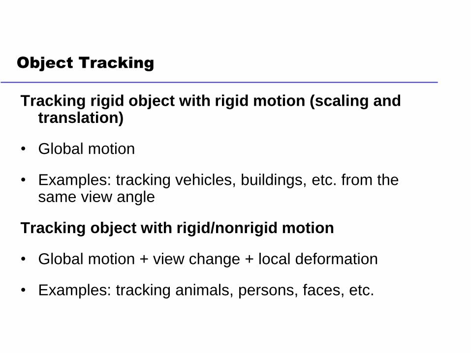
Object Tracking

Tracking rigid object with rigid motion (scaling and translation)

• Global motion

• Examples: tracking vehicles, buildings, etc. from the same view angle

Tracking object with rigid/nonrigid motion

• Global motion + view change + local deformation

• Examples: tracking animals, persons, faces, etc.

Object Tracking – Motion Analysis from Multiple

Frames

Tracking vs optical flow:

• Tracking is often applied for a few specified targets in the video

• Optical flow is applied for any points on the image –dense optical flow

• Both of them need to compute the correspondence between images

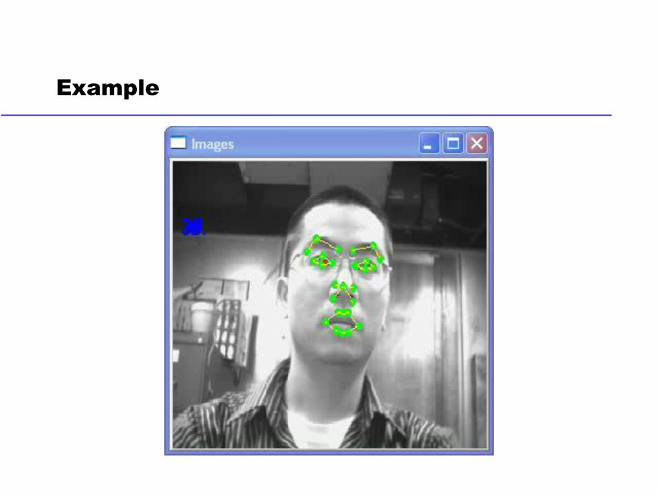
Example

Object Tracking – Motion Analysis from Multiple

Frames

tth frame t+1th frame

(𝑥𝑡 , 𝑦𝑡) (𝑥𝑡+1, 𝑦𝑡+1)

𝒔𝒕

𝒐𝒕

𝒔𝒕+𝟏

𝒐𝒕+𝟏

Question:

Given 𝐬𝒕 and 𝐨𝒕+𝟏 = 𝑥𝑡+1, 𝑦𝑡+1 , how to

estimate 𝐬𝒕+𝟏?

For a point 𝑝 = (𝑥𝑡 , 𝑦𝑡) at the 𝑡𝑡ℎ time frame with a velocity of 𝑣𝑡 =

(𝑣𝑥𝑡 , 𝑣𝑦𝑡), we define a state vector 𝐬𝒕 = 𝑥𝑡 , 𝑦𝑡 , 𝑣𝑥𝑡, 𝑣𝑦𝑡𝑻

𝑣𝑡 = (𝑣𝑥𝑡 , 𝑣𝑦𝑡)p

General Strategy for Object Tracking

Predict position for next frame

Initialization Object Detection

Local search Template matching

Finalize the position

A well-known algorithm following the strategy -- Kalman filter

Tracking – General Probabilistic Formulation

Given

•𝑃(𝐬𝑡|𝐨0, ⋯ , 𝐨𝑡) - “Prior”

We should like to know

•𝑃(𝐬𝑡+1|𝐨0, ⋯ , 𝐨𝑡)- “Predictive distribution”

•𝑃(𝐬𝑡+1|𝐨0, ⋯ , 𝐨𝑡, 𝐨𝑡+1)– “Posterior”

How to compute them?

𝒔𝟎

𝒐𝟎

𝒔𝟏

𝒐𝟏

… 𝒔𝒕

𝒐𝒕

𝒔𝒕+𝟏

𝒐𝒕+𝟏

𝑃 𝐬𝑡+1 𝐨0, ⋯ , 𝐨𝑡 =

𝐬𝑡

𝑃 𝐬𝑡+1, 𝐬𝑡 𝐨0, ⋯ , 𝐨𝑡

=

𝐬𝑡

𝑃 𝐬𝑡+1 𝐬𝑡 , 𝐨0, ⋯ , 𝐨𝑡 ∗ 𝑃(𝐬𝑡|𝐨0, ⋯ , 𝐨𝑡)

Tracking – General Probabilistic Formulation

Given

•𝑃(𝐬𝑡|𝐨0, ⋯ , 𝐨𝑡) - “Prior”

We should like to know

•𝑃(𝐬𝑡+1|𝐨0, ⋯ , 𝐨𝑡)- “Predictive distribution”

•𝑃(𝐬𝑡+1|𝐨0, ⋯ , 𝐨𝑡, 𝐨𝑡+1)– “Posterior”

How to compute them?

𝒔𝟎

𝒐𝟎

𝒔𝟏

𝒐𝟏

… 𝒔𝒕

𝒐𝒕

𝒔𝒕+𝟏

𝒐𝒕+𝟏

𝑃 𝐬𝑡+1 𝐨0, ⋯ , 𝐨𝑡, 𝐨𝑡+1

=𝑃 𝐨𝑡+1 𝐬𝑡+1, 𝐨0 , ⋯ , 𝐨𝑡 ∗𝑃 𝐬𝑡+1 𝐨0, ⋯ , 𝐨𝑡

σ𝐬𝑡+1 𝑃 𝐨𝑡+1 𝐬𝑡+1, 𝐨0 , ⋯ , 𝐨𝑡 ∗𝑃 𝐬𝑡+1 𝐨0, ⋯ , 𝐨𝑡

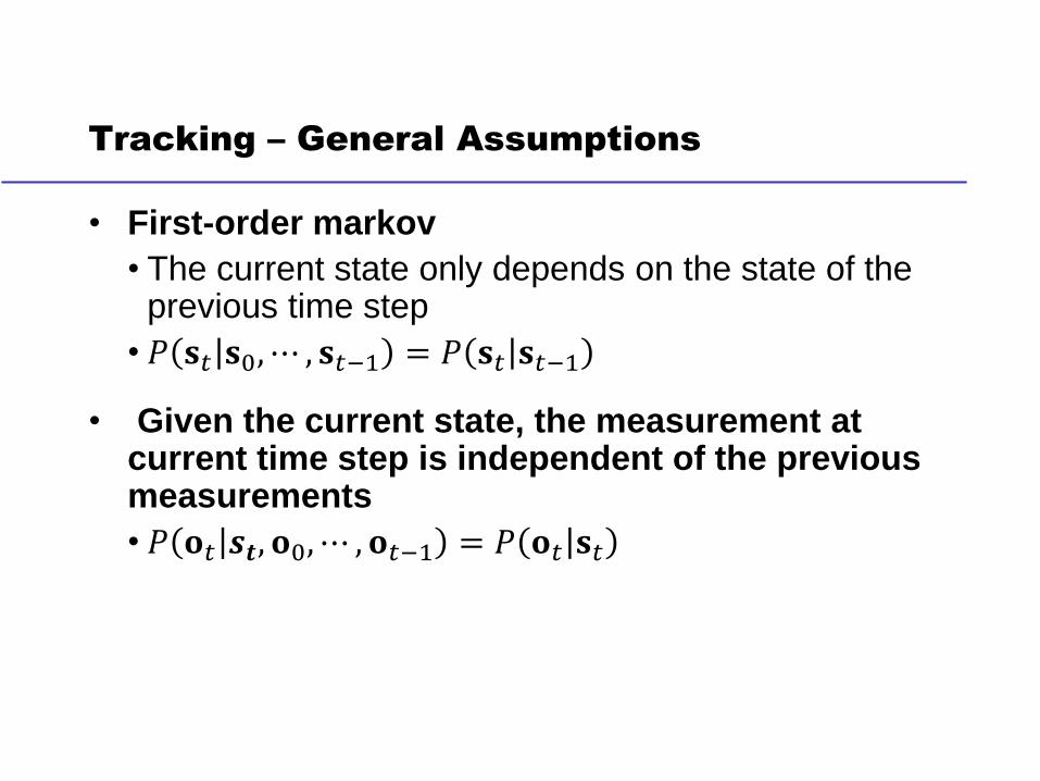
Tracking – General Assumptions

• First-order markov

• The current state only depends on the state of the previous time step

• 𝑃 𝐬𝑡 𝐬0, ⋯ , 𝐬𝑡−1 = 𝑃 𝐬𝑡 𝐬𝑡−1

• Given the current state, the measurement at current time step is independent of the previous measurements

• 𝑃 𝐨𝑡 𝒔𝒕, 𝐨0, ⋯ , 𝐨𝑡−1 = 𝑃 𝐨𝑡 𝐬𝑡

Tracking – General Probabilistic Formulation

𝑃 𝐬𝑡+1 𝐨0, ⋯ , 𝐨𝑡 =

𝐬𝑡

𝑃 𝐬𝑡+1 𝐬𝑡 , 𝐨0, ⋯ , 𝐨𝑡 ∗ 𝑃(𝐬𝑡|𝐨0, ⋯ , 𝐨𝑡)

=

𝐬𝑡

𝑃 𝐬𝑡+1 𝐬𝑡 ∗ 𝑃(𝐬𝑡|𝐨0, ⋯ , 𝐨𝑡)

𝑃 𝐬𝑡+1 𝐨0, ⋯ , 𝐨𝑡, 𝐨𝑡+1 =𝑃 𝐨𝑡+1 𝐬𝑡+1, 𝐨0 , ⋯ , 𝐨𝑡 ∗ 𝑃 𝐬𝑡+1 𝐨0, ⋯ , 𝐨𝑡

σ𝐬𝑡+1 𝑃 𝐨𝑡+1 𝐬𝑡+1, 𝐨0 , ⋯ , 𝐨𝑡 ∗ 𝑃 𝐬𝑡+1 𝐨0, ⋯ , 𝐨𝑡

=𝑃 𝐨𝑡+1 𝐬𝑡+1 ∗ 𝑃 𝐬𝑡+1 𝐨0, ⋯ , 𝐨𝑡

σ𝐬𝑡+1 𝑃 𝐨𝑡+1 𝐬𝑡+1 ∗ 𝑃 𝐬𝑡+1 𝐨0, ⋯ , 𝐨𝑡

Prediction:

Update:

System model

Measurement model

Kalman Filtering

Assumptions

• Linear state model

• The next state 𝐬𝒕+𝟏 is linearly related to the current state 𝐬𝒕

• Uncertainty satisfy a Gaussian

Linear State Model

s𝑡+1 = Φs𝑡 +w𝑡

Φ: state transition matrix

w𝑡: system perturbation satisfying a Gaussian distribution w𝑡~𝑁(0,𝑾)

If motion between two frames is small,

Φ =

1 0 1 00 1 0 10 0 1 00 0 0 1

𝒔𝒕

𝒐𝒕

𝒔𝒕+𝟏

𝒐𝒕+𝟏

Temporal transition

Measurement Model

o𝑡 = Hs𝑡 + r𝑡

• H describes how the measurement relates to the state vector

• For example, 𝐨𝒕 = 𝑥𝑡 , 𝑦𝑡 is the measured feature position

• r𝑡 is the measurement uncertainty satisfying a Gaussian

distribution r𝑡~𝑁(0,𝑹)

𝒔𝒕

𝒐𝒕

𝒔𝒕+𝟏

𝒐𝒕+𝟏

𝐻 =1 0 0 00 1 0 0

The simplest case

Kalman Filtering

Time update:• predict new position

• Predict searching area

Initialization

Local search

Measurement update:• Refine the localization results

• Refine the error

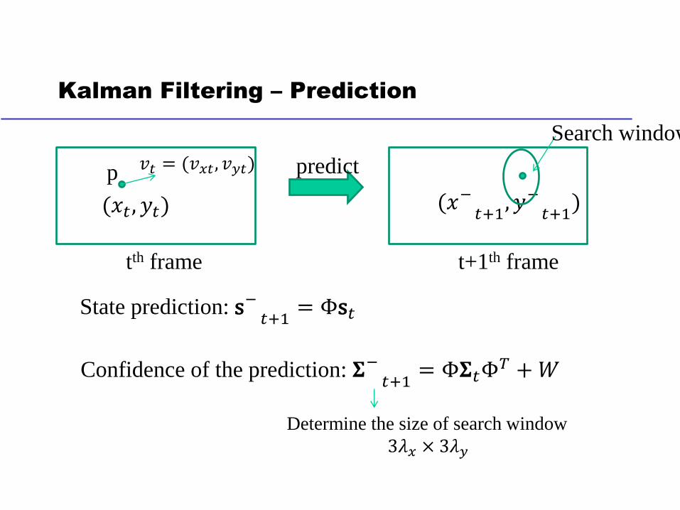
Kalman Filtering – Prediction

tth frame t+1th frame

(𝑥𝑡 , 𝑦𝑡) (𝑥−𝑡+1

, 𝑦−𝑡+1

)

𝑣𝑡 = (𝑣𝑥𝑡 , 𝑣𝑦𝑡)p predict

Search window

State prediction: s−𝑡+1

= Φs𝑡

Confidence of the prediction: 𝚺−𝑡+1

= Φ𝚺𝑡Φ𝑇 +𝑊

Determine the size of search window

3𝜆𝑥 × 3𝜆𝑦

Kalman Filtering – Updating

t+1th frame

(𝑥−𝑡+1

, 𝑦−𝑡+1

)

Searching result

(ො𝑥𝑡+1, ො𝑦𝑡+1)

Kalman gain: 𝐾𝑡+1 = σ𝑡+1− 𝐻𝑇 𝐻σ𝑡+1

− 𝐻𝑇 + 𝑅 −1

t+1th frame

Updating(𝑥𝑡+1, 𝑦𝑡+1)

A weighting factor determines

• the contribution of the measurement and the prediction in

the final estimation -- which one is more reliable

Kalman Filtering – Updating

t+1th frame

(𝑥−𝑡+1

, 𝑦−𝑡+1

)

Searching result

(ො𝑥𝑡+1, ො𝑦𝑡+1)

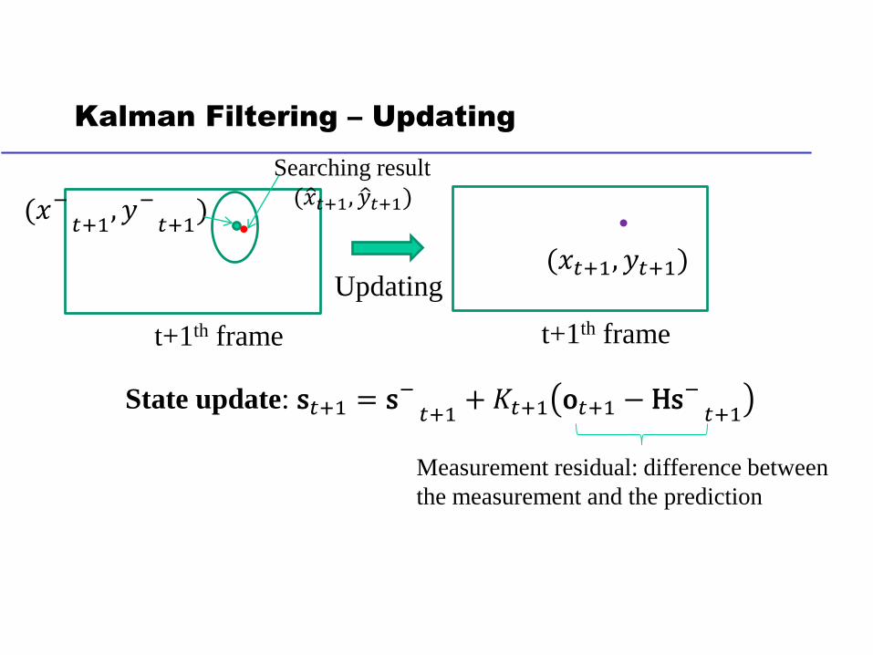
State update: s𝑡+1 = s−𝑡+1

+ 𝐾𝑡+1 o𝑡+1 − Hs−𝑡+1

t+1th frame

Updating(𝑥𝑡+1, 𝑦𝑡+1)

Measurement residual: difference between

the measurement and the prediction

Kalman Filtering – Updating

t+1th frame

(𝑥−𝑡+1

, 𝑦−𝑡+1

)

Searching result

(ො𝑥𝑡+1, ො𝑦𝑡+1)

State update: s𝑡+1 = s−𝑡+1

+ 𝐾𝑡+1 o𝑡+1 − Hs−𝑡+1

t+1th frame

Updating(𝑥𝑡+1, 𝑦𝑡+1)

Error covariance update: Σ𝑡+1 = (𝐼 − 𝐾𝑡+1𝐻)σ𝑡+1−

Kalman Filtering

Time update:• predict new position

• Predict searching area

Initialization

Local search

Measurement update:• Refine the localization results

• Refine the error

𝑅 =4 00 4

𝑊 =

9 0 0 00 9 0 00 0 4 00 0 0 4

s0

Σ0 =

100 0 0 00 100 0 00 0 36 00 0 0 36

Limitation of Kalman Filtering

Failed cases:

• State transition is not linear

• Sudden motion direction/velocity changes

• Uncertainty is not Gaussian

• State vector is not unimodal

• Multiple targets

A new method Particle Filtering

Extended Kalman filtering

Unscented Kalman filtering

Reading Assignments

An Introduction to the Kalman Filter by Welch and Bishop

http://www.cs.unc.edu/~welch/media/pdf/kalman_intro.pdf