Final Plan Attachment 7 - Australian Energy Regulator · ACIL Allen Consulting (ACIL Allen) has...
38
Final Plan Attachment 7.3 Opex Partial Productivity Analysis A Report by ACIL Allen Consulting 20 December 2016
Transcript of Final Plan Attachment 7 - Australian Energy Regulator · ACIL Allen Consulting (ACIL Allen) has...

Final Plan Attachment 7.3 Opex Partial Productivity Analysis
A Report by ACIL Allen Consulting 20 December 2016

Victoria and Albury Final Plan Attachment 7.3 December 2016

REPORT TO
AUSTRALIAN GAS NETWORKS LIMITED
20 DECEMBER 2016
OPEX PARTIAL PRODUCTIVITY ANALYSIS
AUSTRALIAN GAS NETWORKS LIMITED
C O N T E N T S
EXECUTIVE SUMMARY I
1
Introduction 5 1.1 Report structure 5
2
Cost function analysis 6 2.1 Overview of cost function analysis 6 2.2 Model functional form 6 2.3 Econometric approach 9 2.4 Estimation techniques 10
3
Productivity analysis data 14 3.1 Sample of gas distribution businesses 14 3.2 Data limitations and issues 15 3.3 Data definitions 17
4
Estimated costs functions 18 4.1 Cost functions estimated 18 4.2 Model validation and testing 18 4.3 Two output specification: Energy and Customer numbers 20 4.4 Single output specification 22
5
Opex partial productivity growth forecast-single output model 24 5.1 Inputs to calculating opex partial productivity 24 5.2 Calculating opex partial productivity 25 5.3 Opex partial productivity forecasts 25 5.4 Output growth 27
6
Opex partial productivity growth forecasts-two output model 29 6.1 Inputs to calculating opex partial productivity 29 6.2 Calculating opex partial productivity 30 6.3 Opex partial productivity forecasts 31 6.4 Output growth 32
A
References 33
FIGURES FIGURE 5.1 PROJECTED OUTPUT GROWTH RATE, CUSTOMER NUMBERS 27

C O N T E N T S
FIGURE 6.1 PROJECTED OUTPUT GROWTH RATES UNDER FGLS AND SFA MODELS 32
TABLES TABLE ES 1 ANNUAL OPEX PARTIAL PRODUCTIVITY FORECASTS, RANDOM EFFECTS MODEL III TABLE ES 2 ANNUAL OPEX PARTIAL PRODUCTIVITY FORECASTS, FGLS MODEL IV TABLE ES 3 ANNUAL OPEX PARTIAL PRODUCTIVITY FORECASTS, SFA MODEL IV TABLE 4.1 ESTIMATED COBB-DOUGLAS FUNCTION: TWO OUTPUTS 21 TABLE 4.2 SUMMARY OF MODEL VALIDATION PROCESS 21 TABLE 4.3 ESTIMATED COBB-DOUGLAS FUNCTION: SINGLE OUTPUT 22 TABLE 4.4 SUMMARY OF MODEL VALIDATION PROCESS 23 TABLE 5.1 SINGLE OUTPUT OPEX COST FUNCTION REGRESSION ESTIMATE 24 TABLE 5.2 FORECAST CHANGES IN GROWTH DRIVERS 24 TABLE 5.3 ANNUAL OPEX PARTIAL PRODUCTIVITY FORECASTS, RANDOM EFFECTS MODEL 26 TABLE 5.4 ANNUAL OPEX PARTIAL PRODUCTIVITY FORECASTS, FGLS MODEL 26 TABLE 5.5 ANNUAL OPEX PARTIAL PRODUCTIVITY FORECASTS, SFA MODEL 26 TABLE 6.1 TWO OUTPUT OPEX COST FUNCTION REGRESSION ESTIMATE 29 TABLE 6.2 FORECAST CHANGES IN GROWTH DRIVERS 30 TABLE 6.3 ANNUAL OPEX PARTIAL PRODUCTIVITY FORECASTS, FGLS MODEL 31 TABLE 6.4 ANNUAL OPEX PARTIAL PRODUCTIVITY FORECASTS, SFA MODEL 31
OPEX PARTIAL PRODUCTIVITY ANALYSIS AUSTRALIAN GAS NETWORKS LIMITED i
E X E C U T I V E S U M M A R Y
Terms of reference
ACIL Allen Consulting (ACIL Allen) has been engaged by Australian Gas Networks Limited (AGN) to provide productivity analysis in support of the preparation of AGN’s Access Arrangement (AA) proposal for Victoria and Albury for the period 1 January 2018 to 31 December 2022.
This expert report has been prepared to assist AGN to develop expenditure forecasts to be included in the AA proposal. Under the Terms of Reference for the study, ACIL Allen has been asked to provide a forecast of the operating expenditure (opex) partial productivity growth rate that applies to AGN’s Victoria and Albury networks for the period 1 January 2018 to 31 December 2022.
Cost function analysis
In production economics, econometric cost functions provide a useful tool for estimating the least cost means of production and can be used to explore efficient costs for energy networks. A cost function is a function that measures the minimum cost of producing a given set of outputs in a given production environment in a given time period.
By modelling the output quantities, the input prices, and the operating conditions in which the business operates, a minimum-cost function (a theoretical concept), yields an estimate of the periodic costs incurred by an efficient business to deliver those services in that environment.
To facilitate the estimation of econometric cost functions it is necessary to assume a functional or algebraic form that can approximate the unknown, theoretical cost function. The functional form imposes certain assumptions, which may be more or less strict, about the relationships between model variables (outputs, input prices and costs) including relating to economies of scale and elasticities of substitution and hence the shape of the underlying cost function.
The functional forms applied most commonly in the econometric cost benchmarking literature are:
— Cobb-Douglas: a linear in logs functional form that makes relatively stricter assumptions about the functional form
— Translog: a flexible functional form that allows for linear, quadratic and interaction terms in the logarithms of the output quantity and input price variables.
As part of this study we considered both the Cobb Douglas and Translog functional forms as potential options. While the Translog offers extra flexibility, one of the requirements of the specification is a large sample size.
OPEX PARTIAL PRODUCTIVITY ANALYSIS AUSTRALIAN GAS NETWORKS LIMITED ii
Given the small sample size available for this study, we have limited the analysis to the simpler but more restrictive Cobb-Douglas form, where the parameter estimates can be readily interpreted and are reasonably robust to changes in the estimation technique applied.
Sample of gas distribution businesses
The cost function analysis presented in this study uses data from nine Australian gas distribution businesses serving urban populations and that are subject to economic regulation, namely:
— ATCO Gas Australia (WA)
— Australian Gas Networks South Australia (SA) (previously Envestra)
— Australian Gas Networks Victoria (VIC) (previously Envestra)
— Multinet Gas (VIC)
— AusNet Services (VIC)
— Jemena Gas Networks (NSW)
— Australian Gas Networks Queensland (QLD) (previously Envestra)
— Allgas Energy (QLD)
— ActewAGL
ACIL Allen has compiled a dataset for the nine Australian gas distribution businesses. The data were largely sourced from AGN itself and public reports including:
— gas distribution business Access Arrangement Information statements
— regulatory determinations by the AER and jurisdictional regulators
— AER performance reports
— annual and other reports published by the businesses
— consultant reports prepared as part of access arrangement review processes
— Australian Gas Networks who provided an updated set of data for their Victorian and Albury, South Australian and Queensland networks
Data comparability and suitability for the productivity analysis
To a large extent, this study relies on data that were reported publicly by the gas distribution businesses and, in most cases, verified by the relevant economic regulator. Where data has been provided to ACIL Allen directly, the data are reported on a basis that is consistent with the regulatory data in the Access Arrangement Information statements. In particular, the study uses the expenditure categories reported within the gas distribution businesses’ Access Arrangements, including the operating expenditure and capital expenditure categories.
It is our opinion that the data used in the study is robust and appropriate for indicative productivity analysis, particularly as the majority of the data has been subject to scrutiny by the relevant economic regulator and in many cases also by expert consultants engaged by the economic regulators1. There remains, however, some uncertainty about data comparability that cannot be resolved. Possible differences in the comparability of cost categories and other inevitable shortcomings in the analysis mean that the productivity forecasts produced should be treated as indicative, not exact.
By ‘indicative’ we mean that the results of the analysis should be used cautiously, giving careful consideration to the limitations of the dataset and modelling described further below in this section. These limitations suggest that the models parameter estimates will be subject to a degree of uncertainty and that model results should not be regarded as being particularly precise.
Other shortcomings that limit the ability of the models in this study to represent the gas distribution businesses’ true cost functions include:
1 We do however note that the AER in relation to electricity distribution and transmission businesses, require data used for benchmarking purposes to be audited.
OPEX PARTIAL PRODUCTIVITY ANALYSIS AUSTRALIAN GAS NETWORKS LIMITED iii
— the limited data available for this study e.g. a richer data set with a broader range of cost inputs, outputs and operating environment factors could be used to create model specifications that better account for the variation between the gas distribution businesses
— potential data errors that have not been identified
— the limitations of the modelling techniques in terms of their ability to accurately estimate the true opex cost parameters.
Opex partial productivity growth forecasts
Cobb-Douglas cost functions were estimated using two alternative specifications, one with two outputs (energy throughput and customer numbers) and one with a single output (customer numbers) only. The model validation and testing process applied favoured the single output model over the two output model.
Five separate estimation methods were used to estimate the model parameters. These are:
— Pooled ordinary least squares (OLS)
— Fixed effects
— Random effects
— Feasible Generalised Least Squares (FGLS)
— Stochastic frontier analysis (SFA)
The model validation and testing process favoured the FGLS model over the pooled OLS, and the random effects model over the fixed effects model. We therefore excluded the OLS and fixed effects models, and instead focussed on the random effects, FGLS and SFA models in the analysis.
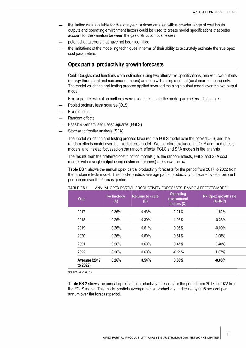
The results from the preferred cost function models (i.e. the random effects, FGLS and SFA cost models with a single output using customer numbers) are shown below.
Table ES 1 shows the annual opex partial productivity forecasts for the period from 2017 to 2022 from the random effects model. This model predicts average partial productivity to decline by 0.08 per cent per annum over the forecast period.
TABLE ES 1 ANNUAL OPEX PARTIAL PRODUCTIVITY FORECASTS, RANDOM EFFECTS MODEL
Year Technology
(A)
Returns to scale
(B)
Operating
environment
factors (C)
PP Opex growth rate
(A+B-C)
2017 0.26% 0.43% 2.21% -1.52%
2018 0.26% 0.39% 1.03% -0.38%
2019 0.26% 0.61% 0.96% -0.09%
2020 0.26% 0.60% 0.81% 0.06%
2021 0.26% 0.60% 0.47% 0.40%
2022 0.26% 0.60% -0.21% 1.07%
Average (2017
to 2022)
0.26% 0.54% 0.88% -0.08%
SOURCE: ACIL ALLEN
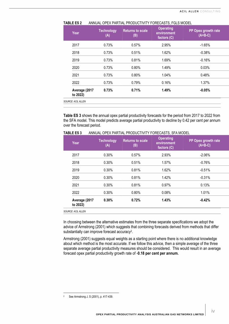
Table ES 2 shows the annual opex partial productivity forecasts for the period from 2017 to 2022 from the FGLS model. This model predicts average partial productivity to decline by 0.05 per cent per annum over the forecast period.
OPEX PARTIAL PRODUCTIVITY ANALYSIS AUSTRALIAN GAS NETWORKS LIMITED iv
TABLE ES 2 ANNUAL OPEX PARTIAL PRODUCTIVITY FORECASTS, FGLS MODEL
Year Technology
(A)
Returns to scale
(B)
Operating
environment
factors (C)
PP Opex growth rate
(A+B-C)
2017 0.73% 0.57% 2.95% -1.65%
2018 0.73% 0.51% 1.62% -0.38%
2019 0.73% 0.81% 1.69% -0.16%
2020 0.73% 0.80% 1.49% 0.03%
2021 0.73% 0.80% 1.04% 0.48%
2022 0.73% 0.79% 0.16% 1.37%
Average (2017
to 2022)
0.73% 0.71% 1.49% -0.05%
SOURCE: ACIL ALLEN
Table ES 3 shows the annual opex partial productivity forecasts for the period from 2017 to 2022 from the SFA model. This model predicts average partial productivity to decline by 0.42 per cent per annum over the forecast period.
TABLE ES 3 ANNUAL OPEX PARTIAL PRODUCTIVITY FORECASTS, SFA MODEL
Year Technology
(A)
Returns to scale
(B)
Operating
environment
factors (C)
PP Opex growth rate
(A+B-C)
2017 0.30% 0.57% 2.93% -2.06%
2018 0.30% 0.51% 1.57% -0.76%
2019 0.30% 0.81% 1.62% -0.51%
2020 0.30% 0.81% 1.42% -0.31%
2021 0.30% 0.81% 0.97% 0.13%
2022 0.30% 0.80% 0.08% 1.01%
Average (2017
to 2022)
0.30% 0.72% 1.43% -0.42%
SOURCE: ACIL ALLEN
In choosing between the alternative estimates from the three separate specifications we adopt the advice of Armstrong (2001) which suggests that combining forecasts derived from methods that differ substantially can improve forecast accuracy2.
Armstrong (2001) suggests equal weights as a starting point where there is no additional knowledge about which method is the most accurate. If we follow this advice, then a simple average of the three separate average partial productivity measures should be considered. This would result in an average forecast opex partial productivity growth rate of -0.18 per cent per annum.
2 See Armstrong J. S (2001), p. 417-439.
OPEX PARTIAL PRODUCTIVITY ANALYSIS AUSTRALIAN GAS NETWORKS LIMITED 5
1 I N T R O D U C T I O N
1 Introduction
ACIL Allen Consulting (ACIL Allen) has been engaged by Australian Gas Networks Limited (AGN) to provide productivity analysis in support of the preparation of AGN’s Access Arrangement (AA) proposal for Victoria and Albury for the period 1 January 2018 to 31 December 2022.
This expert report has been prepared to assist AGN to develop expenditure forecasts to be included in the AA proposal. Under the Terms of Reference for the study, ACIL Allen has been asked to provide a forecast of the operating expenditure (opex) partial productivity growth rate that applies to AGN’s Victoria and Albury networks for the period 1 January 2018 to 31 December 2022.
In ACIL Allen’s view, this involves estimating an opex cost function which is used to calculate an opex partial productivity growth rate forecast split into three components: technology, returns to scale and operating environment.
In conducting the analysis ACIL Allen has had regard to:
— historical and forecast cost, input and output data provided by AGN
— confidential information provided by several Australian gas distribution businesses
— publically available information from other gas distribution businesses, such as regulatory submissions, regulators’ final decisions, and annual reports
1.1 Report structure
The report is structured as follows:
— section 2 provides an overview of cost function analysis including a description of the possible functional forms and estimation techniques used to estimate cost functions
— section 3 describes the data used in the partial productivity analysis including their limitations and deficiencies
— section 4 presents the set of estimated opex cost functions and describes the model selection and validation process
— section 5 calculates the opex partial productivity forecasts based on the most appropriate estimated opex cost functions
— section 6 calculates the opex partial productivity forecasts based on the estimated two output opex cost functions

OPEX PARTIAL PRODUCTIVITY ANALYSIS AUSTRALIAN GAS NETWORKS LIMITED 6
section 3 presents the estimates of AGN’s opex productivity growth rate for the forecast period
2 C O S T F U N C T I O N A N A L Y S I S
2 Cost function analysis
2.1 Overview of cost function analysis
In production economics, econometric cost functions provide a useful tool for estimating the least cost means of production and can be used to explore efficient costs for energy networks. A cost function is a function that measures the minimum cost of producing a given set of outputs in a given production environment in a given time period.
By modelling the output quantities, the input prices, and the operating conditions in which the business operates, a minimum-cost function (a theoretical concept), yields an estimate of the periodic costs incurred by an efficient business to deliver those services in that environment.
Let 𝑥 = (𝑥1, … … , 𝑥𝑀)′, 𝑤 = (𝑤1, … … , 𝑤𝑀)′, 𝑞 = (𝑞1, … … , 𝑞𝑁)′ and 𝑧 = (𝑧1, … … , 𝑧𝐽)′ denote
vectors of input quantities, input prices, output quantities and environmental variables respectively. Mathematically, the cost function is defined as:
𝑐(𝑤, 𝑞, 𝑧, 𝑡)
= 𝑚𝑖𝑛
𝑥 ≥ 0 {𝑤′𝑥: 𝑥 𝑐𝑎𝑛 𝑝𝑟𝑜𝑑𝑢𝑐𝑒 𝑞 𝑖𝑛 𝑎𝑛 𝑒𝑛𝑣𝑖𝑟𝑜𝑛𝑚𝑒𝑛𝑡 𝑐ℎ𝑎𝑟𝑎𝑐𝑡𝑒𝑟𝑖𝑠𝑒𝑑 𝑏𝑦 𝑧 𝑖𝑛 𝑝𝑒𝑟𝑖𝑜𝑑 𝑡}
2.2 Model functional form
To facilitate the estimation of econometric cost functions it is necessary to assume a functional or algebraic form that can approximate the unknown, theoretical cost function. The functional form imposes certain assumptions, which may be more or less strict, about the relationships between model variables (outputs, input prices and costs) including relating to economies of scale and elasticities of substitution and hence the shape of the underlying cost function.
The desirable features of a functional form are as follows:
— it captures the underlying technology of an industry adequately
— it is non-decreasing in prices
― i.e. if prices increase then costs increase
— it is non-decreasing in outputs
― i.e. if outputs increase then costs increase
— homogeneity in prices
― i.e. if you double prices, you double costs
— it has a smooth function
— linearity in its parameters.

OPEX PARTIAL PRODUCTIVITY ANALYSIS AUSTRALIAN GAS NETWORKS LIMITED 7
The functional forms applied most commonly in the econometric cost benchmarking literature are:
— Cobb-Douglas: a linear in logs functional form that makes relatively stricter assumptions about the functional form
— Translog: a flexible functional form that allows for linear, quadratic and interaction terms in the logarithms of the output quantity and input price variables.
In general, increased flexibility in the functional form may be desirable in terms of more closely reflecting reality and allowing for a greater range of possible estimated outcomes. However, the more flexible forms such as a Translog cost function require estimation of a large number of parameters which may introduce econometric problems (e.g. multicollinearity).
A range of practical criteria are typically used to determine the functional form used including reducing estimation problems (including multicollinearity and loss of degrees of freedom when sample size is small), ease of interpretation (some functional forms have an intrinsic and intuitive economic interpretation and in which the functional structure is clear) and computational ease.3
The choice of an appropriate functional form is of vital importance in the estimation of an econometric cost function. If the functional form applied is not appropriate, then the estimated cost function will be mis-specified and any associated opex productivity forecasts will be unreliable.
Cobb-Douglas function
The Cobb-Douglas function assumes a log-linear functional form where the natural logarithm of opex is linear in the logarithm of the output quantities and the input price.
For a Cobb-Douglas function with:
— two output variables:
― energy throughput (E) ― customer numbers (C)
— two input variables:
― capital services proxied by the constant price RAB (R) ― opex price (P)
— a single operating environment variable, customer density (CD)
— a time trend capturing technological changes
the function takes the form:
ln(𝑂𝑝𝑒𝑥) = 𝑎 + 𝑏1𝑇𝑖𝑚𝑒 + 𝑏2 ln(𝐸) + 𝑏3 ln(𝐶) + 𝑏4 ln(𝑃) + 𝑏5 ln(𝑅) + 𝑏6 ln(𝐶𝐷)
To ensure homogeneity in prices, the coefficient on the opex price variable (P), b4 is restricted to equal 1. This is dealt with in the estimation process by subtracting ln(P) from both sides of the equation so that the dependent variable in the regression becomes ln(Opex) minus ln(P) and the price variable disappears from the right hand side of the equation.
The Cobb-Douglas function imposes a constant elasticity of opex to each of the outputs regardless of the scale of the business. From the above specification, this implies that a 1 per cent increase in customer numbers (C) will result in a b3 per cent increase in opex, regardless of whether the firm is large or small.
The sum of the coefficients of the output variables gives an indication of the type of returns to scale present in the sample. If the coefficients b2 and b3 sum to less than 1, operating costs increase at a slower rate than the outputs, implying increasing returns to scale. We would expect this to be the case for gas distribution businesses. This is because gas distribution businesses benefit from increasing efficiency resulting from economies of scale as they move from smaller to larger scale production.
The Cobb-Douglas functional form is useful to the extent that it reflects the underlying production technology of gas distribution businesses which are subject to increasing returns to scale. This functional form has been applied in a number of previous studies of gas distribution businesses.
3 Fuss, M, McFadden D. and Mundlak, Y,”A Survey of Functional Forms in the Economic Analysis of Production” in Fuss, M and McFadden D. (Eds) (1978), Production Economics: A Dual Approach to Theory and Applications.

OPEX PARTIAL PRODUCTIVITY ANALYSIS AUSTRALIAN GAS NETWORKS LIMITED 8
Translog functional form
The Translog functional form allows for linear, quadratic and interaction terms between the output and input variables.
The Translog is an example of a flexible functional form which is considerably less restrictive than the Cobb-Douglas. It allows for linear, quadratic and interaction terms in the natural logarithms of output and input prices. Its main advantage over the Cobb-Douglas is that it allows the degree of returns to scale to vary with firm size, something that the Cobb-Douglas does not allow.
Extending the two output, two input and single environmental variable Cobb-Douglas function above to the more flexible Translog function, we get:
ln(𝑂𝑝𝑒𝑥) = 𝑎 + 𝑏1𝑇𝑖𝑚𝑒 + 𝑏2 ln(𝐸) + 𝑏3 ln(𝐶) + 𝑏4 ln(𝑃) + 𝑏5 ln(𝑅) + 𝑏6 ln(𝐶𝐷) + 0.5𝑏22 ln(𝐸)2 +
𝑏23 ln(𝐸) ln(𝐶) + 0.5𝑏33 ln(𝐶)2 + 0.5𝑏44 ln(𝑃)2 + 0.5𝑏55 ln(𝑅)2 +0.5𝑏66 ln(𝐶𝐷)2 + 𝑏24 ln(𝐸) ln(𝑃) +
𝑏25 ln(𝐸) ln(𝑅) + 𝑏26 ln(𝐸) ln(𝐶𝐷) + 𝑏34 ln(𝐶) ln(𝑃) + 𝑏35 ln(𝐶) ln(𝑅) + 𝑏36 ln(𝐶) ln(𝐶𝐷) +
𝑏45 ln(𝑃) ln(𝑅) + 𝑏46 ln(𝑃) ln(𝐶𝐷) + 𝑏56 ln(𝑅) ln(𝐶𝐷)
In this instance the Translog function requires twenty-one explanatory variables, compared to six for the Cobb-Douglas.
Under certain restrictions, the Translog function reduces to a Cobb Douglas function. This will be the case when the coefficients on all the quadratic and interaction terms are zero.
While the Translog is more suitable due to its flexible form, it becomes unsuitable in the face of a limited sample size. Small samples will have insufficient degrees of freedom to reliably estimate the parameters of the model. Furthermore, there is likely to be strong multicollinearity between the explanatory variables due to numerous terms involving transformations of the same variables and interaction among variables. This problem is exacerbated when the sample size is small.
In the absence of a limited sample size, the translog function’s main advantage is its flexibility. By being less restrictive than the Cobb-Douglas function, its use reduces the risk of model mis-specification that could arise from imposing restrictions on the functional form that are not valid.
Choice of functional form
As part of this study we initially considered both the Cobb Douglas and Translog functional forms as potential options.
While the Translog offers extra flexibility, this is achieved at additional cost. One of the requirements of the Translog specification is a sample size that is large enough to provide sufficient degrees of freedom to reliably estimate the cost function and also to overcome the problem of multicollinearity between the explanatory variables.
For the sample of 90 observations available for this study, which includes a combination of actual information and other estimated/forecast information, the addition of quadratic and interaction terms into a translog specification resulted in significant instability in the parameter estimates.
It is our view that the analysis is limited in this respect and that it should remain focussed on the simpler but more restrictive Cobb-Douglas form, where the parameter estimates can be readily interpreted and are reasonably robust to changes in the estimation technique applied.
As mentioned previously, the main disadvantage of the Cobb-Douglas functional form is the degree of its restrictiveness, for example by imposing the restriction that the percentage response of opex to a given 1% change in an output, is the same whether the firm is large or small. If the restrictions imposed by the Cobb-Douglas are not valid, then the estimated model is mis-specified and the opex productivity forecasts obtained from the model are subject to error.
If the sample size was considerably larger, a less restrictive translog function could be a better choice. Particularly as the Cobb-Douglas function is a special case of the translog, so that if the Cobb-Douglas is the true functional form, the estimated parameters of a translog function should reflect this.

OPEX PARTIAL PRODUCTIVITY ANALYSIS AUSTRALIAN GAS NETWORKS LIMITED 9
2.3 Econometric approach
Different cost function estimation approaches may be applied. This study adopts an econometric approach estimating the opex cost functions. The econometric approach is a parametric approach that aims to establish a statistical relationship between operating costs and the individual cost drivers.
The main advantages of the econometric approach are that it allows for:
— statistical testing to choose between competing models
— differences in operating environment such as scale and density to be controlled for across firms, something which is not possible within many non-parametric methods.
The main disadvantages are:
— the conventional econometric method does not separate statistical noise from inefficiency
― this is where Stochastic Frontier Analysis (SFA) deviates from the conventional econometric approach by attempting to split one from the other through the introduction of a composite error term
— the econometric method is reliant on the functional form of the model to be chosen so as to reflect the appropriate production technology of the firms in question
— it is subject to a number of data limitations and statistical problems which may bias the results.
A large range of possible estimation techniques is possible. In this study we consider pooled OLS, Fixed and random effects models, Feasible GLS and SFA. These are discussed in greater detail in section 2.4.
2.3.1 Choice of variables
The possible output, input and operating environment variables that may be specified from the data available are shown below.
Outputs
— energy throughput (TJ)
— customer numbers
In 2013 Economic Insights4 was commissioned by the AER to provide advice on economic benchmarking of electricity Network Service Providers (NSPs), including the appropriate choice of outputs, inputs and operating environment variables.
The report recommended that any chosen output should reflect services provided to customers and that the output itself should be significant. The report makes a distinction between billed outputs, which are used as the basis for billing customers, such as energy throughput and customers, who pay fixed charges and functional outputs such as system capacity, system reliability and system security.
The report also recommends the use of customer numbers as an output, given that customers pay fixed charges on their bills and that these charges reflect activities that the NSP must undertake regardless of the amount of energy delivered. Economic Insights also recommend the use of energy delivered as an output as it is the service that is directly consumed by the customers. They do note however, that the inclusion of energy delivered is ‘more arguable’ because provided there is sufficient capacity, changes in energy throughput will have only a marginal impact on operating costs.
Economic Insights recommended the use of system capacity as an output variable in the cost function. While we considered mains line length as a possible inclusion, we found the combination of a small sample size and multicollinearity between the three output variables made it impossible to estimate a plausible model with all three outputs.
Finally, we are not in a position to consider the possibility of system reliability or system security related output variables as these data are absent from our dataset. In any case, system reliability and system security are issues that are of greater relevance to electricity rather than gas networks.
4 Economic Insights (2013), Economic Benchmarking of Electricity Network Service Providers, Report prepared for the AER, 25 June 2013.
OPEX PARTIAL PRODUCTIVITY ANALYSIS AUSTRALIAN GAS NETWORKS LIMITED 10
Inputs
— capital services (constant price Regulatory Asset Base (RAB))
— opex price index (weighted price index described below)
While Economic Insights recommended that use of physical measure of input capital services, constant price RAB is used as a proxy for capital instead of mains length mainly to avoid significant multicollinearity issues that arise from the presence of mains length in the denominator of the network density variable.
The opex price index is the index recommended by the AER for network service providers.5 This is a weighted opex price index formed using the following Australian Bureau of Statistics (ABS) indexes and weights:
— electricity, gas, water and waste services (EGWWS) wage price index (WPI) —62 per cent
— intermediate inputs: domestic producer price index (PPI) —19.5 per cent
— data processing, web hosting and electronic information storage PPI —8.2 per cent
— other administrative services PPI —6.3 per cent
— legal and accounting PPI —3 per cent
— market research and statistical services PPI —1 per cent.
ACIL Allen sourced these indexes from the ABS and calculated the weighted index.
Environmental variables
— network density (customers per km of network length)
According to the AER6, the main criteria for selecting an environmental variable should be that it has a material impact, it is exogenous and outside the control of the NSP and that it is a primary driver of costs. Based on these criteria, Economic Insights (2013) states that density variables are likely to be the most important operating environment factors that will affect efficiency comparisons between NSPs. Customer density is therefore an appropriate choice for an environmental variable.
Other possible environmental variables listed by Economic Insights include energy density, weather factors and terrain factors, although the last two are more relevant to electricity than gas. This is because power lines are mainly above ground while gas pipelines are primarily below ground. Energy density was considered as an alternative to customer density in the modelling but found to be inferior in terms of its explanatory power. This means that more of the variability in the opex data could be explained using customer density as an explanatory variable rather than energy density. Multicollinearity issues precluded the use of both in the specified cost functions.
Since the data set used has only one environmental control variable, the likelihood of correct model specification is limited. However, while this does not invalidate the results, it suggests that the results may not be robust enough to rely on deterministically, are subject to a degree of error and need to be interpreted cautiously.
2.4 Estimation techniques
The study tested the following cost function estimation techniques:
— Pooled OLS
— Fixed and random effects models
— Feasible Generalised Least Squares (FGLS)
— Stochastic Frontier Analysis (SFA)
Each of the techniques is discussed below.
5 See AER, 2013, p. 154-155. 6 See AER, 2013, p. 158

OPEX PARTIAL PRODUCTIVITY ANALYSIS AUSTRALIAN GAS NETWORKS LIMITED 11
2.4.1 Pooled OLS
The standard econometric technique to estimate a cost function is ordinary least squares (OLS). OLS fits a linear relationship between the dependent variable and a set of explanatory variables, in our case a set of outputs, inputs and operating environment variables. The line of best fit is chosen so as to minimise the sum of squared errors of the model.
The OLS estimator is considered BLUE (the best linear unbiased estimator) under a set of restrictive assumptions:
— the dependent variable is a linear function of a set of independent variables plus a disturbance term
— the expected value of the disturbance term is zero (unbiasedness)
— disturbances have uniform variance and are uncorrelated (homoscedastic, no serial correlation)
— observations on the independent variables are fixed in repeated samples
— there are no exact linear relationships between independent variables (no perfect multicollinearity).
Pooled OLS treats the entire sample as if it is a single cross section. It does not recognise that the data has two dimensions, both across time and firms. This approach therefore does not recognise the panel structure of the data. This is not an issue if there is no heterogeneity across firms or if the heterogeneity can be captured entirely by existing explanatory variables in the model. However, in this and similar analyses, this is difficult due to the lack of environmental variables and the uncertainty about the comparability of the data. The inability to capture all environmental variables in the model will disadvantage the firm that has higher opex costs that arise due to environmental factors. Such are firm will appear to be inefficient relative to its peers in any productivity benchmarking exercise.
2.4.2 Fixed and random effects models
The panel nature of our dataset has a number of attractive features which can be captured through the application of fixed or random effects models. These are:
— panel data can be used to deal with heterogeneity across firms. There are a large number of unmeasured explanatory variables that will affect the behaviour of each firm. Failure to account for these can lead to bias in estimation.
— by combining both cross section and time series, panel data provides more variation in data which can help to alleviate multicollinearity problems and lead to more efficient estimates.
In the standard fixed effects specification, the unobserved variables that drive the heterogeneity across firms is accounted for by different intercepts for each firm in the estimation. The main drawback of the fixed effects model is the loss of significant degrees of freedom through the implicit inclusion of dummy variables to account for the different intercepts across firms. This leads to less efficient estimates of the common slopes.
The random effects model adopts an alternative way of allowing for different intercepts across firms, which aims to overcome the loss of efficiency that arises in the fixed effect specification.
The random effects model views the different intercepts across firms as having been drawn from a random pool of possible intercepts. The random effects model therefore has a single overall intercept, a set of explanatory variables and a composite error term. The composite error term has two components:
— the random intercept term which measures the extent to which the individual firms intercept differs from the overall intercept
— the conventional error term, which indicates the random disturbance for a given firm in each time period.
The random intercept term is the same for each firm across all time periods.
The random effects estimator saves on degrees of freedom and consequently produces more efficient estimates of the slope coefficients than the fixed effects model. This suggests that the random effects estimator is superior to the fixed effects model. Unfortunately, this is only true if the individual firms’ intercepts are not correlated with any of the explanatory variables. If they are, then the estimated slope coefficients will be biased. While it is not clear how this bias will affect the model parameters, its
OPEX PARTIAL PRODUCTIVITY ANALYSIS AUSTRALIAN GAS NETWORKS LIMITED 12
presence will lead to errors in the estimated coefficients and consequently in the opex productivity forecasts. This is not a problem with the fixed effects estimator because the different intercepts are recognised explicitly.
2.4.3 Feasible GLS (FGLS)
An alternative estimation method to that of OLS is Feasible Generalised Least Squares (FGLS).
OLS estimates are only efficient under the assumption of homoscedasticity and no serial correlation in the residuals. When these assumptions are violated, the OLS estimates are inefficient, although they remain unbiased. By inefficient we mean that the estimator no longer has the minimum variance among the class of linear unbiased estimators.
In this circumstance, the usual formula of the variance-covariance matrix is incorrect and the estimated variance-covariance matrix will be biased. In this context, interval estimation and hypothesis testing can no longer be trusted.
To address these problems, two solutions have been developed.
The first is a set of heteroscedasticity and autocorrelation consistent variance-covariance matrix estimators for the OLS estimator, which eliminate the bias in the variance-covariance matrix (albeit only asymptotically). These then allow OLS and other estimators to be employed with more confidence.
These heteroscedasticity and autocorrelation consistent variance-covariance estimators are sometimes referred to as robust variance estimates. Wherever possible in this study, we present t statistics based on heteroscedasticity and autocorrelation consistent variance-covariance estimators.
Alternatively, another estimator which explicitly recognises the heteroscedasticity and autocorrelation of the disturbances is FGLS, which can produce a linear unbiased estimator with smaller variances than OLS. This is done by using additional information such as that large disturbances are likely to be large because their variances are larger, or that large and positive error values in one period are likely to be followed by large and positive error values in the following period.
While OLS estimation minimises the sum of squared residuals, FGLS minimises an appropriately weighted sum of squared residuals, which gives lower weights to those residuals that are expected to be large because their variance is large or those residuals that are expected to be large because other residuals are large.
This approach results in a more efficient estimator than that obtained through OLS regression under heteroscedasticity or serial correlation. Under the classical OLS assumptions of spherical disturbances, the OLS estimator is the most efficient.
2.4.4 Stochastic Frontier Analysis (SFA)
The standard econometric approach is typically interpreted as all deviations from the predicted values of the model are due to inefficiency. This interpretation is an assumption, whereas in truth, the error term (i.e. ‘deviation’) is due to three causes: measurement error and other statistical noise, firm heterogeneity outside of management control, and managerial inefficiency.
Just like the standard econometric approach, SFA aims to model the relationship between operating costs, outputs and environmental variables. However, SFA separates the error term into two components:
— an inefficiency term, and
— a random error component.
This split attempts to remove the influence of random noise from the estimate of firm inefficiency. However, these two terms can only be interpreted as such if all firm heterogeneity outside of management control is accounted for within the model. If such factors are not taken into account within the model, then this firm heterogeneity will enter, most likely, both terms as well as affect estimates of the other parameters. This will result in errors in the estimated model parameters which will then feed through into the opex productivity growth forecasts.
OPEX PARTIAL PRODUCTIVITY ANALYSIS AUSTRALIAN GAS NETWORKS LIMITED 13
SFA uses maximum likelihood estimation to model the relationship between opex and its drivers. The model takes the form:
where, in the ideal case:
is the opex for firm i at time t
refers to all output and environmental drivers of opex j for firm i at time t
captures the effect of random factors such as unusual weather conditions for firm i at time t
captures the inefficiency for firm i at time t.
The statistical noise term is assumed to follow a normal distribution with mean zero and variance σ2:
𝑣𝑖𝑡~𝑁(0, 𝜎𝑣2)
The inefficiency term is assumed to follow a one-sided non-negative truncated normal distribution with mean μ and variance equal to σ2:
𝑢𝑖𝑡 = 𝑁+(𝜇, 𝜎𝑢2)
It is logical for the inefficiency term to remain positive because a business cannot reduce costs below the minimum possible level for a given set of outputs at a given set of input prices.
Just as in the standard econometric approach, SFA requires additional assumptions about the functional form of the cost function. If the underlying production technology of the industry is not reflected in the choice of cost function, there is a risk that this mis-specification could lead to biased estimates which will introduce errors into the productivity growth forecasts.
Because of the separation of the error term into two separate components, estimation of SFA cost models are more computationally demanding than conventional econometric methods. Moreover, separating the random and inefficiency components of the error term requires a large number of data points. This is a significant drawback in our case, where we have data on only nine firms and a limited number of observations.
𝑥𝑗𝑖𝑡
𝑢𝑖𝑡
𝑣𝑖𝑡
𝐶𝑖𝑡
OPEX PARTIAL PRODUCTIVITY ANALYSIS AUSTRALIAN GAS NETWORKS LIMITED 14
3 P R O D U C T I V I T Y A N A L Y S I S D A T A
3 Productiv ity analys is data
This section describes the sample of Australian gas distribution firms used in the opex productivity analysis. Information is also provided on:
— the sources of the data used in the study
— limitations to data that are available publicly
— qualifications regarding the extent to which ACIL Allen has been able to verify the accuracy and comparability of the data.
3.1 Sample of gas distribution businesses
The cost function analysis presented in this study uses data from nine Australian gas distribution businesses serving urban populations and that are subject to economic regulation, namely:
— ATCO Gas Australia (WA)
— Australian Gas Networks South Australia (SA) (previously Envestra)
— Australian Gas Networks Victoria (VIC) (previously Envestra)
— Multinet Gas (VIC)
— AusNet Services (VIC)
— Jemena Gas Networks (NSW)
— Australian Gas Networks Queensland (QLD) (previously Envestra)
— Allgas Energy (QLD)
— ActewAGL
ACIL Allen has compiled a dataset for the nine Australian gas distribution businesses. The data were largely sourced from AGN itself and public reports including:
— gas distribution business Access Arrangement Information statements
— regulatory determinations by the AER and jurisdictional regulators
— AER performance reports
— annual and other reports published by the businesses
— consultant reports prepared as part of access arrangement review processes
— Australian Gas Networks who provided an updated set of data for their Victorian and Albury, South Australian and Queensland networks
ACIL Allen’s database also contains confidential data from several other Australian gas distribution businesses. Confidential data are not revealed within this report.
OPEX PARTIAL PRODUCTIVITY ANALYSIS AUSTRALIAN GAS NETWORKS LIMITED 15
ACIL Allen has sourced data for the historical period from 2003-04 to 2014-15. Data for all gas distribution businesses is available from 2004-05. Data is available for a subset of the businesses in 2003-04. Over the historical period the study relies to the greatest extent possible on data from reported actual costs and outputs, rather than on forecasts.
The key data items used in the econometric analysis are:
— Customer numbers
— Energy throughput (TJ)
— Mains line length (km)
— Operating expenditures ($m)
— Regulatory Asset Base (RAB)
3.2 Data limitations and issues
3.2.1 Data comparability and suitability for the productivity analysis
To a large extent, this study relies on data that were reported publicly by the gas distribution businesses and, in most cases, verified by the relevant economic regulator. Where data has been provided to ACIL Allen directly, the data are reported on a basis that is consistent with the regulatory data in the Access Arrangement Information statements. In particular, the study uses the expenditure categories reported within the gas distribution businesses’ Access Arrangements, including the operating expenditure and capital expenditure categories.
It is our opinion that the data used in the study is robust and appropriate for indicative productivity analysis, particularly as the majority of the data has been subject to scrutiny by the relevant economic regulator and in many cases also by expert consultants engaged by the economic regulators7. There remains, however, some uncertainty about data comparability that cannot be resolved. Possible differences in the comparability of cost categories and other inevitable shortcomings in the analysis mean that the productivity forecasts produced should be treated as indicative, not exact.
By ‘indicative’ we mean that the results of the analysis should be used cautiously, giving careful consideration to the limitations of the dataset and modelling described further below in this section. These limitations suggest that the models parameter estimates will be subject to a degree of uncertainty and that model results should not be regarded as being particularly precise.
Other shortcomings that limit the ability of the models in this study to represent the gas distribution businesses’ true cost functions include:
— the limited data available for this study e.g. a richer data set with a broader range of cost inputs, outputs and operating environment factors could be used to create model specifications that better account for the variation between the gas distribution businesses
— potential data errors that have not been identified
— the limitations of the modelling techniques in terms of their ability to accurately estimate the true opex cost parameters.
3.2.2 Small number of firms
A key limitation of this study is that the sample includes only nine firms. While other studies have tried to rectify this situation by significantly expanding the sample size to include firms from international jurisdictions, this is likely to exacerbate other problems such as the failure to account for operating differences between jurisdictions.
A larger sample size will help to improve the accuracy of the model parameter estimates. This will be beneficial if the additional businesses are subject to the same regulatory requirements and business conditions to those already in the sample. This is unlikely to be the case if the businesses are from different international jurisdictions. For example, if there is different accounting treatment of operating expenses across jurisdictions, those businesses in jurisdictions where costs are likely to be capitalised
7 We do however note that the AER in relation to electricity distribution and transmission businesses, require data used for benchmarking purposes to be audited.

OPEX PARTIAL PRODUCTIVITY ANALYSIS AUSTRALIAN GAS NETWORKS LIMITED 16
rather than expensed could be advantaged over those businesses in jurisdictions where this is not the case.
3.2.3 Multicollinearity between explanatory variables
An issue arises in the specification of econometric models when there is a high degree of multicollinearity between the explanatory variables in a regression. Multicollinearity is a phenomenon in which the predictor variables in a regression are highly correlated with each other. When this happens, it becomes difficult to measure the impact of any specific variable in the model, despite the model performing reasonably well as a whole.
A model with collinear explanatory variables will tend to be characterised by:
— imprecise coefficient estimates leading to high standard errors and statistical insignificance
— erratic shifts in the coefficients in response to small changes in the model
— the presence of theoretically inconsistent coefficients.
The presence of multicollinearity is problematic because we are attempting to estimate separate elasticities for each variable within a cost function. If these variables do not exhibit sufficient independent variation then it will not be possible to reliably disentangle the separate effects of each variable. The variables in our data set displaying the highest levels of collinearity are customers and mains line length and the regulatory asset base (RAB) and mains line length.
The multicollinearity problems expands exponentially when estimating the Translog cost function, which contains quadratic and interaction terms for each output, input and operating environment term.
For this reason, it is our opinion that the high degree of multicollinearity between explanatory variables and the small sample size make it impossible to reliably estimate a Translog cost function in this instance. We have therefore limited ourselves to the Cobb-Douglas specification, despite its more restrictive functional form.
3.2.4 Different accounting treatment of opex
When modelling opex, different accounting practices for capitalising costs can potentially disadvantage those businesses that capitalise a smaller percentage of their expenditure. These businesses will show higher levels of opex compared to those businesses that capitalise a larger percentage of their expenditure onto their balance sheets.
3.2.5 Missing environmental variables and model mis-specification
Data limitations are such that we are only able to control for a small number of operating environment variables. Failure to control for important environmental or operational differences can potentially lead to biased results. The key operating environment variable specified in the cost functions is customer density. In previous benchmarking studies of gas distribution businesses this has been shown to be a significant explanator of differences in operating and capital costs8.
Economic Insights (2014) included additional operating environment variables related to network age (proxied by the proportion of mains length not made of cast iron or unprotected steel) and service area dispersion (proxied by the number of city gates). ACIL Allen do not have the data necessary to include these additional operating environment variables. The exclusion of these environmental variables, and potentially other significant operating environment variables could reduce the accuracy of the inefficiency measure that can be attributed to actions of the gas distribution businesses. However, this is not in itself a reason to discount the cost function analysis in this report, but suggests that some care be exercised in the degree of precision that is attached to the model estimates.
8 See for example Economic Insights (2012), “Econometric Estimates of the Victorian Gas Distribution Businesses’ Efficiency and Future Productivity Growth’, Report Prepared for SP Ausnet, 28 March 2012 and Economic Insights (2015), Relative Opex Efficiency and Forecast Opex Productivity Growth of Jemena Gas Networks, Report Prepared for Jemana Gas Networks, 25 February 2015.
OPEX PARTIAL PRODUCTIVITY ANALYSIS AUSTRALIAN GAS NETWORKS LIMITED 17
3.3 Data definitions
The following describes the data items used in the analysis.
Operating expenditure
The operating expenditure amounts used in this benchmarking study reflect the costs classified as operating expenditure within each businesses’ Access Arrangement. This typically includes a range of operating costs (including network operations, regulatory costs and billing cost), maintenance costs (including for pipelines, meters and network control) and other management and administration costs.
As had been identified in previous benchmarking reports, unaccounted for gas (UAFG) is treated differently between the jurisdictions. As a result, it has been excluded from operating costs for this study. Debt raising costs have also been removed where included in reported operating expenditure. This has also been done to account for differences in the treatment of these costs over time and between the businesses. Other operating expenditure items removed to aid comparability and to remove costs that are outside the control of the gas distribution businesses are carbon costs and government levies.
The operating expenditure data sourced for the study were reported in a range of nominal and constant dollar values within the source documents. All dollar amounts have been placed on a common basis using the Australian Bureau of Statistics All Groups, Weighted average of eight capital cities, CPI (Series ID: A2325846C).
Regulatory asset base (RAB)
The measure of RAB is the closing value for each year.
Network length
The network length for the gas distribution businesses includes the mains that the businesses classify as low, medium and high pressure distribution mains and transmission pressure mains operated above 1,050kPa.
Customers
The customer number measure is the total number of customers including residential and non-residential volume customers and contract customers.
Gas delivered
The gas delivered measure is the total gas delivered to the above customers measured in Terajoules (TJ).
Further data requirements associated with the individual modelling approaches are discussed within the relevant sections of the report.
OPEX PARTIAL PRODUCTIVITY ANALYSIS AUSTRALIAN GAS NETWORKS LIMITED 18
4 E S T I M A T E D C O S T S F U N C T I O N S
4 Estimated costs function s
4.1 Cost functions estimated
Five separate estimation methods were applied to our Cobb-Douglas operating cost function. These are:
— pooled ordinary least squares (OLS)
— fixed effects
— random effects
— feasible GLS (FGLS) (with heteroscedastic panels)
— Stochastic Frontier Analysis (SFA) (with time invariant inefficiency).
The results of all five methods are presented in section 4.3 and 4.4. The results presented in section 4.3 are for a model specification including two outputs (energy, which is measured as TJ of gas throughput and customers) and in section 4.4 for a model specification with a single output (customers).
Before presenting the estimated regression models themselves, we describe the model validation and testing process undertaken to choose the most appropriate models for the purpose of forecasting opex partial productivity.
4.2 Model validation and testing
In order to assess the suitability of the various estimated opex cost functions a number of assessment criteria are applied. These are:
1. theoretical coherence- Estimated coefficient signs make economic sense
2. statistical testing and performance- Estimated coefficients are statistically significant and the model fit is good
3. robustness to changes in estimation technique- Estimated coefficients are stable across estimation techniques
The above steps can be considered part of a validation process where each step should be satisfied before a model specification is accepted. Each of the steps are described in more detail below.
4.2.1 Theoretical coherence
In assessing the suitability of any model, it is important that the selected model is consistent with economic theory. This means that the model should contain the theoretical drivers of operating costs as well as variables that control for operating conditions between firms.
OPEX PARTIAL PRODUCTIVITY ANALYSIS AUSTRALIAN GAS NETWORKS LIMITED 19
The estimated coefficients on each of the explanatory variables must have a theoretically correct sign. That is, increases in drivers such as energy throughput or customers must lead to increases in predicted operating costs from the model. If they do not, then the model is not consistent with economic theory and can be considered suspect.
Similarly, the customer density of the gas network is expected to have a negative relationship to operating expenses. As the network grows denser, a given level of outputs is able to be produced at a lower cost compared to a network with lower customer density. Evidence confirming this relationship has been observed in a number of econometric studies9.
The magnitude of the coefficients should also be consistent with our expectations of the production technology of the industry. We would expect there to be economies of scale with regard to opex in the gas distribution business. This is both logical and supported by a significant number of empirical studies of both gas and electricity distribution businesses.
Increasing returns to scale with respect to opex implies that the sum of output coefficients is less than one.
4.2.2 Statistical testing
Statistical significance of estimated coefficients
An important step in assessing the suitability of any explanatory variable is its statistical significance. Not only should the variable be of a sign and magnitude that is consistent with economic theory, but standard hypothesis testing should indicate that the variable is statistically significant either at the 1% or 5% significance levels, though it is preferable to achieve statistical significance at the 1% significance level. The significance level can be interpreted as the probability of rejecting the null hypothesis that no relationship exists between the explanatory and dependent variable when it is actually true. This means that under the 1% level of statistical significance there is only a 1% probability of concluding that a relationship exists when it does not, while the probability of incorrectly concluding that a relationship exists is five times as large at the 5% level of statistical significance. The 1% level of statistical significance therefore provides a considerably higher degree of confidence that our conclusions are actually true. While the 1% level of statistical significance provides a higher level of confidence, both the 1% and 5% levels of statistical significance are used in common practice.
A statistically significant result is one which is unlikely to have occurred by chance. Each estimated coefficient in the regression models has an associated t-statistic or p value. If the estimated p value is less than 0.01 then that coefficient is statistically significant at the 1 per cent significance level. A p-value that is less than 0.05 is significant at the 5 per cent level of significance. The lower the observed p value on a coefficient the greater the probability that a statistically significant relationship exists between the dependent variable and the explanatory variable concerned.
In this study we consider the statistical significance of each variable at both the 1% and 5% levels of statistical significance as a guide to whether a particular variable should be included in a given model. However, it is important to note that in small samples, which we are limited by in this study, it may be difficult to achieve statistical significance for a variable even though the variable is economically significant. This means that some professional judgement needs to be applied where a variable is failing to achieve the desired level of statistical significance but the coefficient estimate is still consistent with economic theory and with other empirical studies. In this instance we may choose to retain the variable in the model even if it fails to satisfy statistical significance.
Goodness of fit
The most commonly used measure of the goodness of fit of a linear regression model to the observed data is the coefficient of determination, also known as R2. It represents the proportion of the variation
9 See for example Economic Insights (2012), “Econometric Estimates of the Victorian Gas Distribution Businesses’ Efficiency and Future Productivity Growth’, Report Prepared for SP Ausnet, 28 March 2012 and Economic Insights (2015), Relative Opex Efficiency and Forecast Opex Productivity Growth of Jemena Gas Networks, Report Prepared for Jemana Gas Networks, 25 February 2015.
OPEX PARTIAL PRODUCTIVITY ANALYSIS AUSTRALIAN GAS NETWORKS LIMITED 20
in the dependent variable that is explained by variation in the independent variables. In assessing a model’s suitability and fitness for purpose, we would prefer the within sample fit to be strong.
However, in the model validation process, the R2 is just one of a wide suite of tools available. While it is important to emphasize that goodness of fit is a desirable feature of any model, there are factors other than in sample fit that need to be taken into account. For example, a high R2 is no guarantee that a model will have any predictive ability.
Testing for fixed and random effects
To choose between pooled OLS, random and fixed effects a number of statistical tests are available.
To test between OLS and a random effects model, we apply the Breusch-Pagan10 Lagrange multiplier test. This tests the null hypothesis that variance across firms is zero and that there is no significant difference across firms. In other words, there is no panel effect. Failure to reject the null hypothesis results in the conclusion that there are no significant differences across firms and that pooled OLS can be justified.
If the null hypothesis is rejected, then the random effects model is preferred to simple OLS.
The Hausman test11 is applied to test if the random effects estimator is unbiased. The Hausman test allows you to decide between a fixed or random effects model, where the null hypothesis supports the random effects model. The test works by testing whether the error terms are correlated with the explanatory variables, a key requirement under the random effects model. If the null hypothesis is not rejected then the random effects model is preferred over the fixed effects model.
Tests for heterogeneity and serial correlation
Additional statistical tests are carried out to assess the presence of heteroscedasticity and autocorrelation in the model residuals. To test for heteroscedasticity, we apply a Modified Wald test for groupwise heteroscedasticity12. Serial correlation is tested for via the Wooldridge Lagrange Multiplier (LM)13 test for autocorrelation in panel data.
4.2.3 Robustness to changes in estimation method
The estimated coefficients should be reasonably stable across a range of estimation techniques. Very large deviations in the coefficients across different models, particularly where the coefficients become theoretically implausible is a sign that the model may not be correctly specified or that the technique is not the most appropriate to use.
4.3 Two output specification: Energy and Customer numbers
Table 4.1 shows the results of the estimated Cobb-Douglas cost functions with two outputs, energy (TJ of gas throughput) and customer numbers. The table shows the estimated coefficients for each of the estimation techniques in column 2 to column 6. Column 1 shows the relevant variable that the coefficient applies to. The numbers in parentheses under each coefficient estimate are the standard errors that apply to each estimate.
A key characteristic of these models is that the energy throughput variable has a negative coefficient under the fixed and random effects models. This is inconsistent with economic theory. Moreover, the coefficient on the energy throughput variable is not statistically significant at the 1% or 5% per cent level of statistical significance in any of the five models. In the cases where the energy throughput coefficient is positive, it remains very small relative to the customer numbers coefficient so that the output weights between customers and energy would be almost entirely skewed towards customers and away from energy. In the pooled OLS model the output weight for customers is 99.6%. In the case of the FGLS and SFA models, the customer numbers output weights would be 93.1% and 98.1% respectively.
10 Breusch, T and A. Pagan (1980) 11 Hausman, J. A. (1978) 12 See Greene (2000) 13 Wooldridge, J.M (2002)

OPEX PARTIAL PRODUCTIVITY ANALYSIS AUSTRALIAN GAS NETWORKS LIMITED 21
These results mean that the two output Cobb-Douglas specification is almost identical to the single output model with customer numbers as the output and would produce very similar opex partial productivity forecasts to the single output model.
These results suggest that energy (gas throughput) is not a key driver of increasing operating expenses for the nine gas distribution businesses under consideration. As a result, an additional model specification is estimated excluding energy throughput.
TABLE 4.1 ESTIMATED COBB-DOUGLAS FUNCTION: TWO OUTPUTS
Variables Pooled OLS Fixed Effects Random effects FGLS SFA
Time -0.0052413 -0.0172452 -0.0047792 -0.0061516 -0.0026175
(0.0047879) (0.0164914) (0.0052286) (0.0038965) (0.0039132)
Customers 0.5673089*** 1.668821*** 0.7620549*** 0.5628946*** 0.5741936***
(0.0602933) (0.4906491) (0.2249678) (0.0545376) (0.06687)
Energy 0.0025814 -0.2530541 -0.0741655 0.0416569 0.0113698
(0.0553899) (0.2197008) (0.137213) (0.049655) (0.073544)
RAB 0.417243*** -0.0069068 0.3162894* 0.3911824*** 0.4068752***
(0.0680399) (0.2369968) (0.1790108) (0.0618976) (0.1128186)
Density -0.4892936*** -1.251097*** -0.6515275*** -0.4987829*** -0.5398125***
(0.0729667) (0.2640096) (0.1922273) (0.068174) (0.1575708)
Constant 1.42338 19.90151 0.0943736 3.138341 -3.890091
(9.654658) (26.67963) (10.26842) (7.782321) (7.80986)
Observations 90 90 90 90 90
R-squared 97.39 93.64 96.95
Number of firms 9 9 9 9 9
Note: Robust standard errors in parentheses,
*** p<0.01, ** p<0.05, * p<0.1
Table 4.2 below summarises the results of the model validation process. The table shows that the two output model including both the energy throughput and customer numbers variables fails to satisfy all three validation tests.
TABLE 4.2 SUMMARY OF MODEL VALIDATION PROCESS
Validation test Result Comment
Theoretical coherence Fail Energy throughput variable has negative coefficient under the fixed and random effects models. This is inconsistent with economic theory.
Statistical testing and performance
Fail The coefficient on the energy throughput variable is not statistically significant at the 1% or 5% level of statistical significance. Statistical testing favours random effects model over fixed effects model. Statistical testing favours FGLS over pooled OLS model. Customer numbers and customer density are both statistically significant at the 1 % level of significance in all models. The time trend representing technical change does not satisfy statistical significance in any of the estimated models. RAB is statistically significant at the 1% significance level in the FGLS and SFA models, but not in the random effects model.
OPEX PARTIAL PRODUCTIVITY ANALYSIS AUSTRALIAN GAS NETWORKS LIMITED 22
Validation test Result Comment
Robustness to changes in estimation technique
Fail Energy throughput variable flips from positive to negative between models
SOURCE: ACIL ALLEN
4.4 Single output specification
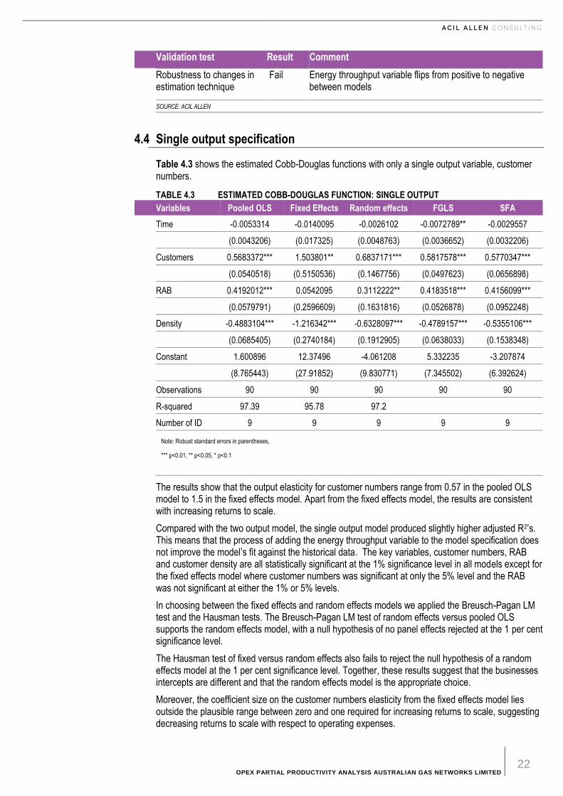
Table 4.3 shows the estimated Cobb-Douglas functions with only a single output variable, customer numbers.
TABLE 4.3 ESTIMATED COBB-DOUGLAS FUNCTION: SINGLE OUTPUT
Variables Pooled OLS Fixed Effects Random effects FGLS SFA
Time -0.0053314 -0.0140095 -0.0026102 -0.0072789** -0.0029557
(0.0043206) (0.017325) (0.0048763) (0.0036652) (0.0032206)
Customers 0.5683372*** 1.503801** 0.6837171*** 0.5817578*** 0.5770347***
(0.0540518) (0.5150536) (0.1467756) (0.0497623) (0.0656898)
RAB 0.4192012*** 0.0542095 0.3112222** 0.4183518*** 0.4156099***
(0.0579791) (0.2596609) (0.1631816) (0.0526878) (0.0952248)
Density -0.4883104*** -1.216342*** -0.6328097*** -0.4789157*** -0.5355106***
(0.0685405) (0.2740184) (0.1912905) (0.0638033) (0.1538348)
Constant 1.600896 12.37496 -4.061208 5.332235 -3.207874
(8.765443) (27.91852) (9.830771) (7.345502) (6.392624)
Observations 90 90 90 90 90
R-squared 97.39 95.78 97.2
Number of ID 9 9 9 9 9
Note: Robust standard errors in parentheses,
*** p<0.01, ** p<0.05, * p<0.1
The results show that the output elasticity for customer numbers range from 0.57 in the pooled OLS model to 1.5 in the fixed effects model. Apart from the fixed effects model, the results are consistent with increasing returns to scale.
Compared with the two output model, the single output model produced slightly higher adjusted R2’s. This means that the process of adding the energy throughput variable to the model specification does not improve the model’s fit against the historical data. The key variables, customer numbers, RAB and customer density are all statistically significant at the 1% significance level in all models except for the fixed effects model where customer numbers was significant at only the 5% level and the RAB was not significant at either the 1% or 5% levels.
In choosing between the fixed effects and random effects models we applied the Breusch-Pagan LM test and the Hausman tests. The Breusch-Pagan LM test of random effects versus pooled OLS supports the random effects model, with a null hypothesis of no panel effects rejected at the 1 per cent significance level.
The Hausman test of fixed versus random effects also fails to reject the null hypothesis of a random effects model at the 1 per cent significance level. Together, these results suggest that the businesses intercepts are different and that the random effects model is the appropriate choice.
Moreover, the coefficient size on the customer numbers elasticity from the fixed effects model lies outside the plausible range between zero and one required for increasing returns to scale, suggesting decreasing returns to scale with respect to operating expenses.

OPEX PARTIAL PRODUCTIVITY ANALYSIS AUSTRALIAN GAS NETWORKS LIMITED 23
Testing for group-wise heteroscedasticity rejected the null hypothesis of no heteroscedasticity at the 1 per cent significance level. The Wooldridge test of serial autocorrelation in panel data failed to reject the null hypothesis of no autocorrelation. These results provide evidence in support of group wise heteroscedasticity in the panel, but not of autocorrelation.
For this reason, we prefer the FGLS model which accounts for heteroscedasticity in the panel over the pooled OLS model which imposes an assumption of homoscedasticity on the disturbances.
In the subsequent section of this report, we do not use the results for the pooled OLS model or the fixed effects models to generate the opex partial productivity forecasts, instead focussing on the random effects, FGLS and SFA models.
Table 4.4 below summarises the results of the model validation process. The table shows that single output model with customer numbers only is better able to withstand the model validation process than the two output model. Although Table 4.4 shows that the single output model does not pass all the validation process steps for all estimation techniques, once the fixed effects and pooled OLS estimation techniques are invalidated by statistical testing, the results strongly favour the single output model over the two output model (which includes throughput as an output variable).
TABLE 4.4 SUMMARY OF MODEL VALIDATION PROCESS
Validation test Result Comment
Theoretical coherence Pass All variables produced signs consistent with economic theory except for customer numbers in the fixed effects model whose value of 1.5 (>1) suggests decreasing rather than increasing returns to scale.
Statistical testing and performance
Pass Statistical testing favours random effects model over fixed effects model. Statistical testing favours FGLS over OLS. Customer numbers and customer density variables are statistically significant at the 1% significance level in each of the random effects, FGLS and SFA models. RAB is statistically significant at the 1% significance level in the FGLS and SFA models and at the 5% significance level in the random effects model. The time variable representing productivity growth arising from technical change is found to be statistically significant at the 5% significance level in the FGLS model only. However, we choose to retain this variable in the model as its inclusion is consistent with economic theory and other empirical studies.
Robustness to changes in estimation technique
Pass Apart from the fixed effects model (which is rejected in favour of the random effects model), the parameter estimates display a reasonable degree of stability.
SOURCE: ACIL ALLEN
OPEX PARTIAL PRODUCTIVITY ANALYSIS AUSTRALIAN GAS NETWORKS LIMITED 24
5 O P E X P A R T I A L P R O D U C T I V I T Y G R O W T H F O R E C A S T -S I N G L E O U T P U T M O D E L
5 Opex partial productiv ity growth forecast-single output model
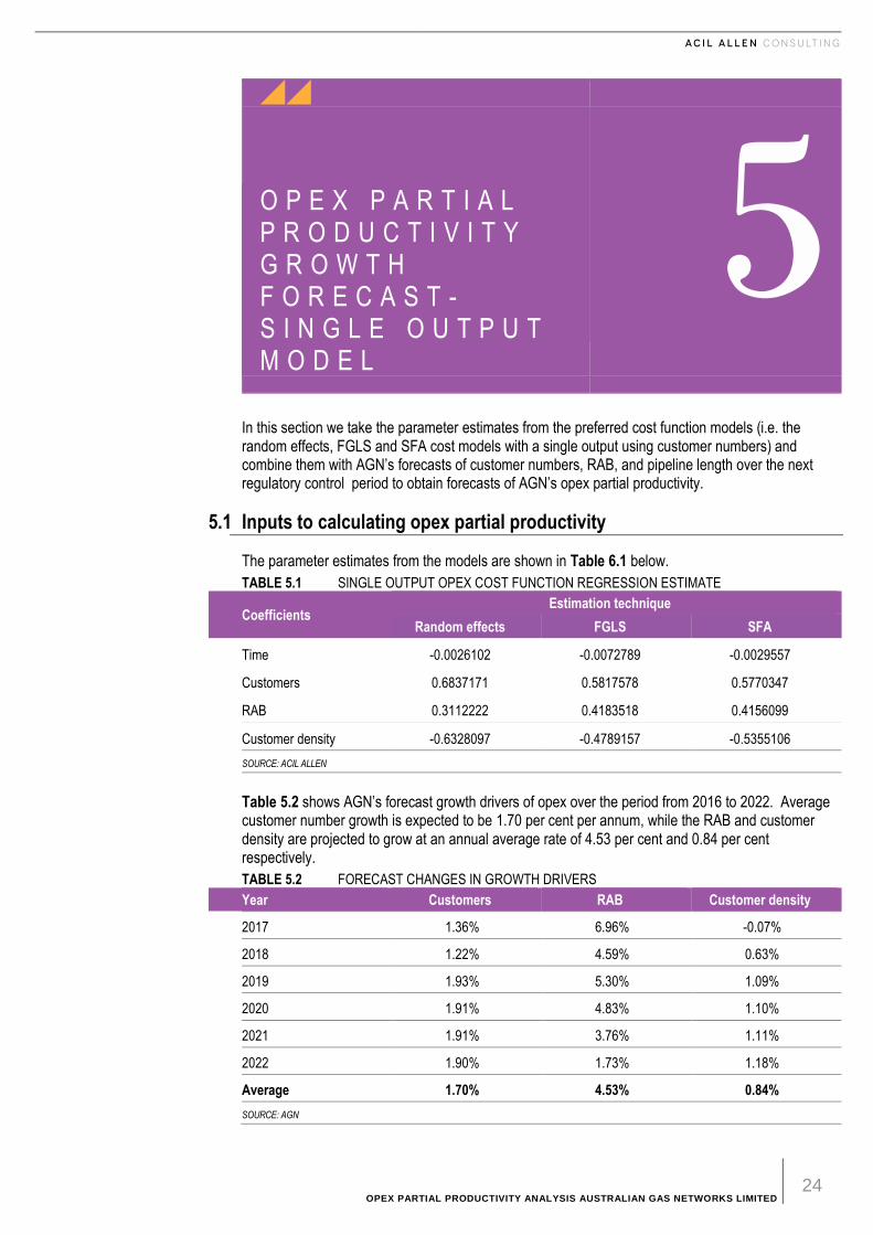
In this section we take the parameter estimates from the preferred cost function models (i.e. the random effects, FGLS and SFA cost models with a single output using customer numbers) and combine them with AGN’s forecasts of customer numbers, RAB, and pipeline length over the next regulatory control period to obtain forecasts of AGN’s opex partial productivity.
5.1 Inputs to calculating opex partial productivity
The parameter estimates from the models are shown in Table 6.1 below.
TABLE 5.1 SINGLE OUTPUT OPEX COST FUNCTION REGRESSION ESTIMATE
Coefficients Estimation technique
Random effects FGLS SFA
Time -0.0026102 -0.0072789 -0.0029557
Customers 0.6837171 0.5817578 0.5770347
RAB 0.3112222 0.4183518 0.4156099
Customer density -0.6328097 -0.4789157 -0.5355106
SOURCE: ACIL ALLEN
Table 5.2 shows AGN’s forecast growth drivers of opex over the period from 2016 to 2022. Average customer number growth is expected to be 1.70 per cent per annum, while the RAB and customer density are projected to grow at an annual average rate of 4.53 per cent and 0.84 per cent respectively.
TABLE 5.2 FORECAST CHANGES IN GROWTH DRIVERS
Year Customers RAB Customer density
2017 1.36% 6.96% -0.07%
2018 1.22% 4.59% 0.63%
2019 1.93% 5.30% 1.09%
2020 1.91% 4.83% 1.10%
2021 1.91% 3.76% 1.11%
2022 1.90% 1.73% 1.18%
Average 1.70% 4.53% 0.84%
SOURCE: AGN
OPEX PARTIAL PRODUCTIVITY ANALYSIS AUSTRALIAN GAS NETWORKS LIMITED 25
The growth in customer density is derived from forecast customer numbers and line length.
5.2 Calculating opex partial productivity
Following Economic Insights (2014), ACIL Allen calculate the partial opex partial productivity growth rate and its three components, namely:
— technical change
— returns to scale
— changes in operating environment.
Technical change is represented by the time trend in the regression. It has a negative coefficient and represents the percentage decrease in opex every year as a result of technological change. This may be due to actual technology, but also encompasses improvements in work practices and methods that lead to lower opex over time.
The productivity gains associated with technical change (A) is estimated as:
𝑇𝑒𝑐ℎ𝑛𝑜𝑙𝑜𝑔𝑦 (𝐴) = −𝑇𝑖𝑚𝑒 𝑐𝑜𝑒𝑓𝑓𝑐𝑖𝑒𝑛𝑡
Returns to scale are productivity gains that arise as a result of increasing business size over time. The productivity gains from returns to scale (B) are calculated as:
For example, if the customer elasticity is 0.5, then a 1% increase in customer numbers would mean that operating expenses would increase by only 0.5%, so that the productivity increase attributable to economies of scale is 0.5%. If the customer elasticity is 1.0, the business has constant returns to scale and the impact of a 1% change in customer numbers on productivity derived from returns to scale would be zero.
Operating environment partial productivity is calculated as the RAB and customer density coefficients multiplied by each of their respective changes in each year. The total operating environment contribution to opex partial productivity is the negative of the sum of the RAB and customer density contributions.
𝑂𝑝𝑒𝑟𝑎𝑡𝑖𝑛𝑔 𝑒𝑛𝑣𝑖𝑟𝑜𝑛𝑚𝑒𝑛𝑡 𝑓𝑎𝑐𝑡𝑜𝑟𝑠 (𝐶) = (𝑅𝐴𝐵 𝑒𝑙𝑎𝑠𝑡𝑖𝑐𝑖𝑡𝑦 × %∆ 𝑖𝑛 𝑅𝐴𝐵) +
(𝐶𝑢𝑠𝑡𝑜𝑚𝑒𝑟 𝑑𝑒𝑛𝑠𝑖𝑡𝑦 𝑒𝑙𝑎𝑠𝑡𝑖𝑐𝑖𝑡𝑦 × %∆ 𝑖𝑛 𝐶𝑢𝑠𝑡𝑜𝑚𝑒𝑟 𝑑𝑒𝑛𝑠𝑖𝑡𝑦)
The opex partial factor productivity growth rate is estimated from these three elements, using the formula:
Opex partial productivity growth rate = A (Technology) + B (Returns to scale) –
C (Operating environment factors)
The operating environment factors are deducted in the above formula because we need to compensate the distribution business that requires higher capital inputs or has a lower customer density than the average firm. For example, a reduction in customer density will have a positive impact on the operating environment factor (C). This is because the customer density elasticity has a negative coefficient. The larger operating environment factor (C) is then deducted from the opex partial productivity growth rate, resulting in a lower opex productivity growth rate.
5.3 Opex partial productivity forecasts
In this section we calculate opex partial productivity forecasts using AGN’s projected growth drivers.
Table 5.3 shows the annual opex partial productivity forecasts for the period from 2017 to 2022 from the random effects model. This model predicts average partial productivity to decrease by 0.08 per cent per annum over the forecast period.
𝑅𝑒𝑡𝑢𝑟𝑛𝑠 𝑡𝑜 𝑠𝑐𝑎𝑙𝑒 (𝐵) = (1 − 𝐶𝑢𝑠𝑡𝑜𝑚𝑒𝑟 𝑒𝑙𝑎𝑠𝑡𝑖𝑐𝑖𝑡𝑦) × (𝑃𝑒𝑟𝑐𝑒𝑛𝑡𝑎𝑔𝑒 𝑐ℎ𝑎𝑛𝑔𝑒 𝑖𝑛 𝑐𝑢𝑠𝑡𝑜𝑚𝑒𝑟𝑠)
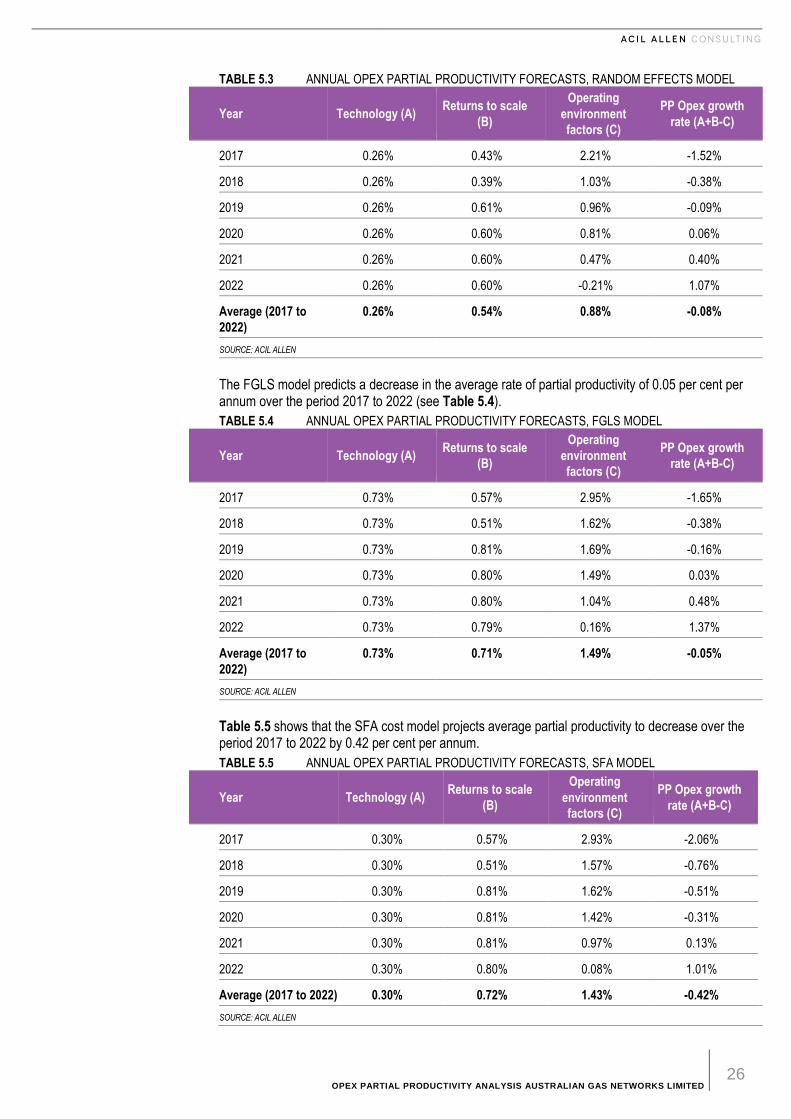
OPEX PARTIAL PRODUCTIVITY ANALYSIS AUSTRALIAN GAS NETWORKS LIMITED 26
TABLE 5.3 ANNUAL OPEX PARTIAL PRODUCTIVITY FORECASTS, RANDOM EFFECTS MODEL
Year Technology (A) Returns to scale
(B)
Operating
environment
factors (C)
PP Opex growth
rate (A+B-C)
2017 0.26% 0.43% 2.21% -1.52%
2018 0.26% 0.39% 1.03% -0.38%
2019 0.26% 0.61% 0.96% -0.09%
2020 0.26% 0.60% 0.81% 0.06%
2021 0.26% 0.60% 0.47% 0.40%
2022 0.26% 0.60% -0.21% 1.07%
Average (2017 to
2022)
0.26% 0.54% 0.88% -0.08%
SOURCE: ACIL ALLEN
The FGLS model predicts a decrease in the average rate of partial productivity of 0.05 per cent per annum over the period 2017 to 2022 (see Table 5.4).
TABLE 5.4 ANNUAL OPEX PARTIAL PRODUCTIVITY FORECASTS, FGLS MODEL
Year Technology (A) Returns to scale
(B)
Operating
environment
factors (C)
PP Opex growth
rate (A+B-C)
2017 0.73% 0.57% 2.95% -1.65%
2018 0.73% 0.51% 1.62% -0.38%
2019 0.73% 0.81% 1.69% -0.16%
2020 0.73% 0.80% 1.49% 0.03%
2021 0.73% 0.80% 1.04% 0.48%
2022 0.73% 0.79% 0.16% 1.37%
Average (2017 to
2022)
0.73% 0.71% 1.49% -0.05%
SOURCE: ACIL ALLEN
Table 5.5 shows that the SFA cost model projects average partial productivity to decrease over the period 2017 to 2022 by 0.42 per cent per annum.
TABLE 5.5 ANNUAL OPEX PARTIAL PRODUCTIVITY FORECASTS, SFA MODEL
Year Technology (A) Returns to scale
(B)
Operating
environment
factors (C)
PP Opex growth
rate (A+B-C)
2017 0.30% 0.57% 2.93% -2.06%
2018 0.30% 0.51% 1.57% -0.76%
2019 0.30% 0.81% 1.62% -0.51%
2020 0.30% 0.81% 1.42% -0.31%
2021 0.30% 0.81% 0.97% 0.13%
2022 0.30% 0.80% 0.08% 1.01%
Average (2017 to 2022) 0.30% 0.72% 1.43% -0.42%
SOURCE: ACIL ALLEN
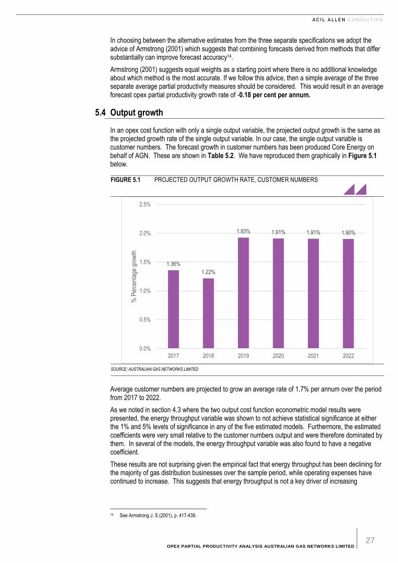
OPEX PARTIAL PRODUCTIVITY ANALYSIS AUSTRALIAN GAS NETWORKS LIMITED 27
In choosing between the alternative estimates from the three separate specifications we adopt the advice of Armstrong (2001) which suggests that combining forecasts derived from methods that differ substantially can improve forecast accuracy14.
Armstrong (2001) suggests equal weights as a starting point where there is no additional knowledge about which method is the most accurate. If we follow this advice, then a simple average of the three separate average partial productivity measures should be considered. This would result in an average forecast opex partial productivity growth rate of -0.18 per cent per annum.
5.4 Output growth
In an opex cost function with only a single output variable, the projected output growth is the same as the projected growth rate of the single output variable. In our case, the single output variable is customer numbers. The forecast growth in customer numbers has been produced Core Energy on behalf of AGN. These are shown in Table 5.2. We have reproduced them graphically in Figure 5.1 below.
FIGURE 5.1 PROJECTED OUTPUT GROWTH RATE, CUSTOMER NUMBERS
SOURCE: AUSTRALIAN GAS NETWORKS LIMITED
Average customer numbers are projected to grow an average rate of 1.7% per annum over the period from 2017 to 2022.
As we noted in section 4.3 where the two output cost function econometric model results were presented, the energy throughput variable was shown to not achieve statistical significance at either the 1% and 5% levels of significance in any of the five estimated models. Furthermore, the estimated coefficients were very small relative to the customer numbers output and were therefore dominated by them. In several of the models, the energy throughput variable was also found to have a negative coefficient.
These results are not surprising given the empirical fact that energy throughput has been declining for the majority of gas distribution businesses over the sample period, while operating expenses have continued to increase. This suggests that energy throughput is not a key driver of increasing
14 See Armstrong J. S (2001), p. 417-439.
1.36%
1.22%
1.93% 1.91% 1.91% 1.90%
0.0%
0.5%
1.0%
1.5%
2.0%
2.5%
2017 2018 2019 2020 2021 2022
% P
erce
ntag
e gr
owth

OPEX PARTIAL PRODUCTIVITY ANALYSIS AUSTRALIAN GAS NETWORKS LIMITED 28
operating expenses for the nine gas distribution businesses under consideration and is therefore excluded as an output from the econometric specification and any subsequent calculations.
OPEX PARTIAL PRODUCTIVITY ANALYSIS AUSTRALIAN GAS NETWORKS LIMITED 29
6 O P E X P A R T I A L P R O D U C T I V I T Y G R O W T H F O R E C A S T S - T W O O U T P U T M O D E L
6 Opex partial productiv ity growth forecasts -two output model
While our preferred model in this study is the single output model using customer numbers, for the sake of completeness, in this section we also present the opex partial productivity growth forecasts based on the two output model using both customer numbers and energy throughput as outputs.
We do this by taking the parameter estimates from the two output cost function models (i.e. the FGLS and SFA cost models) and combine them with AGN’s forecasts of customer numbers, energy throughput, RAB, and pipeline length over the next regulatory control period to obtain forecasts of AGN’s opex partial productivity.
6.1 Inputs to calculating opex partial productivity
The parameter estimates from the models are shown in Table 6.1 below. Please note that the random effects model is excluded from the suite of estimation techniques because it produced a negative coefficient for the energy throughput variable.
Table 6.1 also shows the output weights implied by the regression estimates. In the case of the FGLS model, customer numbers receive an output weight of 93.1% while energy throughput has a weight of 6.9%. In the case of the SFA model, customer numbers receive an output weight of 98.1%, with energy throughput receiving an output weight of only 1.9%.
TABLE 6.1 TWO OUTPUT OPEX COST FUNCTION REGRESSION ESTIMATE
Estimation technique
Coefficients FGLS SFA
Time -0.0061516 -0.0026175
Customers 0.5628946 0.5741936
Energy 0.0416569 0.0113698
RAB 0.3911824 0.4068752
Customer density -0.4987829 -0.5398125
Output weights
Customers 93.11% 98.06%
Energy 6.89% 1.94%
Table 6.2 shows AGN’s forecast growth drivers of opex over the period from 2017 to 2022. Average customer number and growth is expected to be 1.70 per cent per annum, while energy throughput is expected to decline by 0.06% per annum. Applying the output weights from the estimated regressions, the average weighted output growth from the FGLS model is expected to be 1.58% per
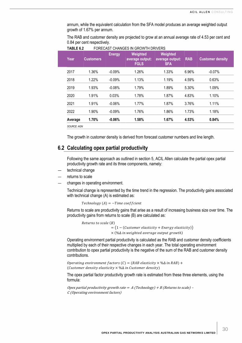
OPEX PARTIAL PRODUCTIVITY ANALYSIS AUSTRALIAN GAS NETWORKS LIMITED 30
annum, while the equivalent calculation from the SFA model produces an average weighted output growth of 1.67% per annum.
The RAB and customer density are projected to grow at an annual average rate of 4.53 per cent and 0.84 per cent respectively.
TABLE 6.2 FORECAST CHANGES IN GROWTH DRIVERS
Year Customers
Energy Weighted
average output:
FGLS
Weighted
average output:
SFA
RAB Customer density
2017 1.36% -0.09% 1.26% 1.33% 6.96% -0.07%
2018 1.22% -0.09% 1.13% 1.19% 4.59% 0.63%
2019 1.93% -0.08% 1.79% 1.89% 5.30% 1.09%
2020 1.91% 0.03% 1.78% 1.87% 4.83% 1.10%
2021 1.91% -0.06% 1.77% 1.87% 3.76% 1.11%
2022 1.90% -0.09% 1.76% 1.86% 1.73% 1.18%
Average 1.70% -0.06% 1.58% 1.67% 4.53% 0.84%
SOURCE: AGN
The growth in customer density is derived from forecast customer numbers and line length.
6.2 Calculating opex partial productivity
Following the same approach as outlined in section 5, ACIL Allen calculate the partial opex partial productivity growth rate and its three components, namely:
— technical change
— returns to scale
— changes in operating environment.
Technical change is represented by the time trend in the regression. The productivity gains associated with technical change (A) is estimated as:
𝑇𝑒𝑐ℎ𝑛𝑜𝑙𝑜𝑔𝑦 (𝐴) = −𝑇𝑖𝑚𝑒 𝑐𝑜𝑒𝑓𝑓𝑐𝑖𝑒𝑛𝑡
Returns to scale are productivity gains that arise as a result of increasing business size over time. The productivity gains from returns to scale (B) are calculated as:
𝑅𝑒𝑡𝑢𝑟𝑛𝑠 𝑡𝑜 𝑠𝑐𝑎𝑙𝑒 (𝐵)
= (1 − (𝐶𝑢𝑠𝑡𝑜𝑚𝑒𝑟 𝑒𝑙𝑎𝑠𝑡𝑖𝑐𝑖𝑡𝑦 + 𝐸𝑛𝑒𝑟𝑔𝑦 𝑒𝑙𝑎𝑠𝑡𝑖𝑐𝑖𝑡𝑦))
× (%∆ 𝑖𝑛 𝑤𝑒𝑖𝑔ℎ𝑡𝑒𝑑 𝑎𝑣𝑒𝑟𝑎𝑔𝑒 𝑜𝑢𝑡𝑝𝑢𝑡 𝑔𝑟𝑜𝑤𝑡ℎ)
Operating environment partial productivity is calculated as the RAB and customer density coefficients multiplied by each of their respective changes in each year. The total operating environment contribution to opex partial productivity is the negative of the sum of the RAB and customer density contributions.
𝑂𝑝𝑒𝑟𝑎𝑡𝑖𝑛𝑔 𝑒𝑛𝑣𝑖𝑟𝑜𝑛𝑚𝑒𝑛𝑡 𝑓𝑎𝑐𝑡𝑜𝑟𝑠 (𝐶) = (𝑅𝐴𝐵 𝑒𝑙𝑎𝑠𝑡𝑖𝑐𝑖𝑡𝑦 × %∆ 𝑖𝑛 𝑅𝐴𝐵) +
(𝐶𝑢𝑠𝑡𝑜𝑚𝑒𝑟 𝑑𝑒𝑛𝑠𝑖𝑡𝑦 𝑒𝑙𝑎𝑠𝑡𝑖𝑐𝑖𝑡𝑦 × %∆ 𝑖𝑛 𝐶𝑢𝑠𝑡𝑜𝑚𝑒𝑟 𝑑𝑒𝑛𝑠𝑖𝑡𝑦)
The opex partial factor productivity growth rate is estimated from these three elements, using the formula:
Opex partial productivity growth rate = A (Technology) + B (Returns to scale) –
C (Operating environment factors)
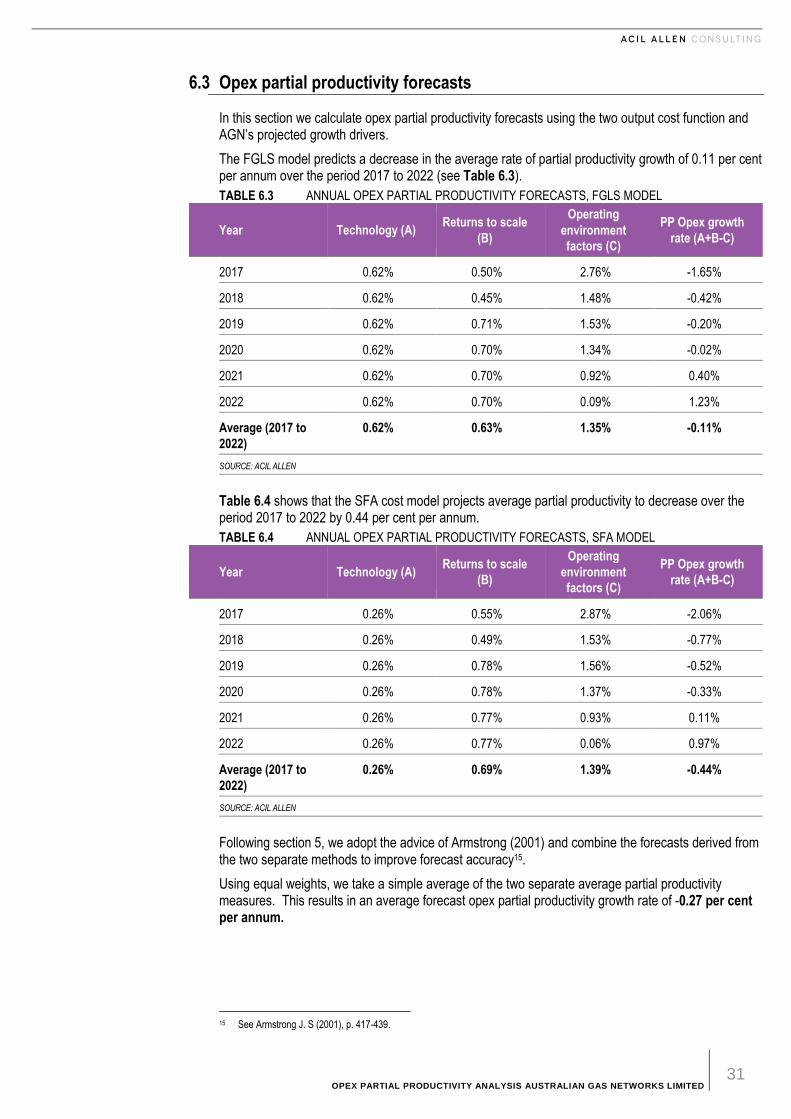
OPEX PARTIAL PRODUCTIVITY ANALYSIS AUSTRALIAN GAS NETWORKS LIMITED 31
6.3 Opex partial productivity forecasts
In this section we calculate opex partial productivity forecasts using the two output cost function and AGN’s projected growth drivers.
The FGLS model predicts a decrease in the average rate of partial productivity growth of 0.11 per cent per annum over the period 2017 to 2022 (see Table 6.3).
TABLE 6.3 ANNUAL OPEX PARTIAL PRODUCTIVITY FORECASTS, FGLS MODEL
Year Technology (A) Returns to scale
(B)
Operating
environment
factors (C)
PP Opex growth
rate (A+B-C)
2017 0.62% 0.50% 2.76% -1.65%
2018 0.62% 0.45% 1.48% -0.42%
2019 0.62% 0.71% 1.53% -0.20%
2020 0.62% 0.70% 1.34% -0.02%
2021 0.62% 0.70% 0.92% 0.40%
2022 0.62% 0.70% 0.09% 1.23%
Average (2017 to
2022)
0.62% 0.63% 1.35% -0.11%
SOURCE: ACIL ALLEN
Table 6.4 shows that the SFA cost model projects average partial productivity to decrease over the period 2017 to 2022 by 0.44 per cent per annum.
TABLE 6.4 ANNUAL OPEX PARTIAL PRODUCTIVITY FORECASTS, SFA MODEL
Year Technology (A) Returns to scale
(B)
Operating
environment
factors (C)
PP Opex growth
rate (A+B-C)
2017 0.26% 0.55% 2.87% -2.06%
2018 0.26% 0.49% 1.53% -0.77%
2019 0.26% 0.78% 1.56% -0.52%
2020 0.26% 0.78% 1.37% -0.33%
2021 0.26% 0.77% 0.93% 0.11%
2022 0.26% 0.77% 0.06% 0.97%
Average (2017 to
2022)
0.26% 0.69% 1.39% -0.44%
SOURCE: ACIL ALLEN
Following section 5, we adopt the advice of Armstrong (2001) and combine the forecasts derived from the two separate methods to improve forecast accuracy15.
Using equal weights, we take a simple average of the two separate average partial productivity measures. This results in an average forecast opex partial productivity growth rate of -0.27 per cent per annum.
15 See Armstrong J. S (2001), p. 417-439.

OPEX PARTIAL PRODUCTIVITY ANALYSIS AUSTRALIAN GAS NETWORKS LIMITED 32
6.4 Output growth
In a two output cost function model the output growth is calculated as the weighted average of the two individual output growth rates, in this case customer numbers and energy throughput.
The customer numbers and energy throughput growth forecasts were developed by Core Energy on behalf of AGN. These are shown in Table 6.2. The weighted average output growth rate is then calculated using the relative coefficient sizes from the econometric models as the output weights. In the FGLS model, customer numbers receive an output weight of 93.1%. This is calculated by taking the coefficient for customers (0.5629) and dividing it by the sum of the energy and customer coefficients (0.60455). The output weight for energy from the FGLS model is 6.9%, and is simply equal to 1 minus the customer numbers output weight.
In the SFA model, a similar process results in an output weight for customer numbers of 98.1% and 1.9% for energy throughput.
The projected output growth rates using the output weights from the FGLS and SFA regression models are shown in Figure 6.1. Over the period from 2017 to 2022, the average rate of output growth from the FGLS and SFA models is expected to be 1.58% and 1.67% respectively.
FIGURE 6.1 PROJECTED OUTPUT GROWTH RATES UNDER FGLS AND SFA MODELS
SOURCE: ACIL ALLEN
1.26%1.13%
1.79% 1.78% 1.77% 1.76%
1.33%1.19%
1.89% 1.87% 1.87% 1.86%
0.00%
0.20%
0.40%
0.60%
0.80%
1.00%
1.20%
1.40%
1.60%
1.80%
2.00%
2017 2018 2019 2020 2021 2022
Weighted average output growth: FGLS Weighted average output growth: SFA
OPEX PARTIAL PRODUCTIVITY ANALYSIS AUSTRALIAN GAS NETWORKS LIMITED 33
A . R E F E R E N C E S
A References
ACIL Allen (2015), Productivity Study: ActewAGL Distribution Gas Network, 29 April 2015.
AER, 2013, Better Regulation, Expenditure Forecast Assessment Guideline for Electricity Distribution, November
Armstrong J. S, (2001), Principals of forecasting: A Handbook for Researchers and Practitioners, Kluver Academic Publishing
Breusch, T and A. Pagan, (1980), The LM Test and Its Application to Model specification in Econometrics, Review of Economic Studies, 47 p 239-254
Economic Insights (2012), “Econometric Estimates of the Victorian Gas Distribution Businesses’ Efficiency and Future Productivity Growth’, Report Prepared for SP Ausnet, 28 March 2012
Economic Insights (2013), Economic Benchmarking of Electricity Network Service Providers, Report prepared for the AER, 25 June 2013
Economic Insights (2014), Relative Opex Efficiency and Forecast Opex Productivity Growth of Jemena Gas Networks, Report prepared for Jemena Gas Networks, 14 April
Economic Insights (2015), Relative Opex Efficiency and Forecast Opex Productivity Growth of Jemena Gas Networks, Report Prepared for Jemana Gas Networks, 25 February 2015.
Fuss, M, McFadden D. and Mundlak, Y,”A Survey of Functional Forms in the Economic Analysis of Production” in Fuss, M and McFadden D. (Eds) (1978), Production Economics: A Dual Approach to Theory and Applications
Greene, (2000), Econometric Analysis, Upper Saddle River, NJ: Prentice-Hall
Hausman, J. A., (1978), Specification tests in econometrics, Econometrics 46: 1251-1271
Wooldridge, J.M, (2002), Econometric Analysis of Cross Section and Panel Data. Cambridge, MA: MIT Press