Final Hall

7/24/2019 Final Hall

http://slidepdf.com/reader/full/final-hall 1/29

The transport of charges investigated by Hall

Effect

Simon Lacoste-Julien

Mathieu Plamondon

Lab Report

Department of Physics

McGill University

April 15th, 2002

Abstract

Voltages across a germanium crystal are recorded on a range of tem-peratures going from 150 to 383 K. Impurities, temperature and the pres-ence of a magnetic field (causing the Hall effect and magnetoresistance)modify the mechanism of conduction. Measurements of the temperaturedependence of the resistivity ρ together with the Hall coefficient RH giveinformation on several properties of the semiconductor. The n-type natureof the dopant has been successfully established and its concentration, ap-

proached by a factor of two. The bandgap energy E g measured was foundin the right range of expected values. Finally, two types of charge carriers’mobilities were discriminated and the power law of ρ(T ) in the intrinsicregion was verified, as well as the power law for ρ(B) (magnetoresistance).

1



1 Introduction

The 20th century has been the theater of deep transformations all domains:politics, arts, science,... The revolution in the communications and computerswill surely become its principal legacy. This was initiated by the discovery of the transistor and its technologic development since 1947. These devices arebased on junctions of semiconductors into which a current can flow in a uniquedirection. The physics behind such peculiarity is a direct consequence of theQuantum Mechanics. The properties of the semiconductors revealing a wealthof possibilities, a new branch was born: the Solid State Physics.

However, the first insights on the theory of conduction into materials camefrom Edwin Hall who found in 1879 an effect which has his name. He remarkedthat a voltage appears across crystal’s sides when it is inserted into a magneticfield and a current passes through it. A successful explanation was given by con-sidering the deflection of the charge carriers due to the magnetic force. Today,

the Hall Effect combined with the knowledge of the resistivity of a semiconduc-tor can be used to deduce many of its properties: the process of intrinsic andextrinsic conduction, the nature of the dopant, the concentration of impuritycarriers, the conduction mechanism, the bandgap and the mobility of the carri-ers. Using a germanium crystal, the aim of this experiment is to illustrate howsuch measurements yield to all this information.

2 Theory

2.1 Band structure in crystals

The first property describing a material is its ability to transport charges under

the influence of an applied electric field E . This situation is governed by Ohm’sLaw (see [1]): J = σ E (1)

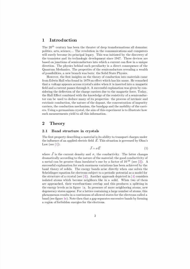
where J is the current density and σ, the conductivity. The latter changesdramatically according to the nature of the material: the good conductivity of a metal can be greater than insulator’s one by a factor of 10 24 (see [2]). Asuccessful explanation for such enormous variations has been achieved by theband theory of solids. The energy bands arise directly when one solves theSchrodinger equation for electrons subject to a periodic potential as a model forthe structure of a crystal (see [3]). Another approach depicted in [4] considersisolated atoms which become neighbors like in a solid. When two of themare approached, their wavefunctions overlap and this produces a splitting in

the energy levels as in figure 1a. In presence of more neighboring atoms, newdegeneracy states appear. For a lattice containing a large number of atoms, thisphenomenon results in a continuum of allowed states for the electrons called aband (see figure 1c). Note then that a gap separates successive bands by forminga region of forbidden energies for the electrons.

2



Figure 1: Splitting of the energy levels due to atomic lattice. [2, p.435]

We shall see that the occupation and the position of the two highest bandscompletely determines the conductivity of a solid. The valence band is theoutermost containing electrons while the lowest one which possesses availablestates is called the conduction band. The separation between the two corre-sponds to the energy gap E g of the material. As shown in figure 2, this valueindicates the nature of conduction. In metals, no gap exists and electrons canmove freely because the unoccupied states just above are attained with a smallamount of additional energy. On the other hand, insulators possess large en-

ergy gaps (∼ 10 eV) compared to kBT at room temperature (0.025 eV), wherekB is the Boltzmann constant. The Fermi-Dirac distribution predicts that atnormal temperatures very few electrons can be thermally excited to the upperband, resulting in a low conductivity. The semi-conductors lie between thosetwo extremes and thus have very interesting properties.

2.2 Semiconductors and impurities

The energy gap for semiconductors is of the order of 1 eV. At low temperatures,they remain poor conductors as no electrons populates the conduction band.However, as the temperature increases, the thermal excitation through the nar-row gap becomes more probable. The conductivity is thus expected to increaseat sufficiently hight temperature.

A particularity for semiconductors is that both positive and negative chargecarriers are present. When an electron is promoted from the valence band to theconduction band (see figure 3), it leaves behind a vacant crystal site, so-calledhole. This electron-deficient site in the otherwise filled valence band acts like apositive charge: a nearby valence electron transfers to this empty site, leavinga hole behind, at its original place. This process is repeated and the hole

3



Figure 2: Energy band diagrams for different kinds of solids. [2, p.437-438] a) conductor (metal) b) insulator c) semi-conductor

Figure 3: Flow of charge carriers in a pure semi-conductor excited by

an electric field. [2, p.439]

4



Figure 4: Energy band diagrams for two kinds of doping of a semi-

conductor. [2, p.443-444] a) p-typed doping b) n-typed doping

migrates through the valence band. In pure crystals, the number n of negativecharge carriers has to equal p, the number of positive ones. The transport of this pair of charges created by thermal excitation in a semiconductors has aname: intrinsic conduction . With a high energy approximation (i.e. E kBT )(see [5]), n is described by a Boltzmann distribution:

n 2πmekBT

h2

3

2

exp−E g/2kBT (2)

All important semiconductors are tailored to the needs of a particular deviceby a process called doping. It consists of an addition of specific impurities tothe structure of the crystal. According to their effect, we subdivide them intwo categories. A donor is an impurity lying at an energy E d just below theconduction band and capable of donating electrons to it (see figure 4a). Sincethe charge carriers are negative electrons, the semiconductor is known as ann-type. Alternatively, we can insert acceptor atoms as in figure 4 which acceptelectrons from the valence band just below. Now the charge is carried by positiveholes, giving a p-type crystal. The conduction due to any of these impuritiesis called extrinsic and as a first consequence, the symmetry in the number of charge carriers is lost. i.e. n = p. Making a low temperature approximation,the number of electrons in the conduction band is given by

n = N d

2πmekBT

h2

3

2

exp−E d/2kBT (3)

where N d corresponds to the number of donors. In the case of the germanium,

5



a separation E d of 0.01eV has a relatively small kBT energy associated with itin comparison to an E g of 0.67eV [5, p.82]. Hence, for temperatures T 120 K ,

the number of impurity carriers in the conduction band becomes saturated ( n N d). As the temperature increases, these act like a constant number of freeelectrons and there is a gradual increase of the density of intrinsic carriers [ 5,p.82-83].

2.3 Resistivity

The types of the charge carriers and conduction have been exposed. The nextstep considers the quantitative temperature dependence of the transport of charges. For this purpose, we rather use the dual quantity ρ, the resistivityof the material, which is defined as the inverse of the conductivity. This macro-scopic property is linked to the motion of the charges in the crystal. When nofield is applied, an electron executes a free path between collisions, moving in arandom fashion as a molecule in a gas. Under the influence of a field E , it driftsin the direction given by the field. The drift velocity vd is related to the field’sstrength by:

vd = µ E (4)

where the proportionality constant µ is called the mobility. The current densityrestricted to one dimension can be expressed as a function of the velocity of thecharges by:

J = envd (5)

e being the fundamental charge. Combining Equations 1 to 4, we obtain thisrelation for the resistivity if one type of carriers is present in the semi-conductor:

ρ(T ) =

1

σ ∝

1

µ T

−3

2

exp

E g

2kBT (6)

In the extrinsic region, the density of carriers remains almost constant and apower law is expected [5, p.92]:

ρext(T ) ∝ T β (7)

where β is a constant. Combining (4), (5) and (7), the behaviour of the driftmobility µd linked to the drift velocity and the resistivity goes like:

µd ∝ 1

ρext∝ T −β (8)

Furthermore, considering some approximations about the thermal velocity of

the charge carriers and their mean free path, we can derive as in [ 5] a simpleapproximation for the temperature dependence of the resistivity and we getβ = 3/2 for the region of constant n:

µd ∝ T −3

2 (9)

6



For larger T, in the intrinsic dominated region, the behaviour of (6) becomesdominated by the exponential:

ρint(T ) ∝ exp E g2kBT

(10)

On the other hand, the resistivity can also be measured directly in terms of the resistance R of the whole sample and its geometry:

R = ρ

A (11)

where A is the cross-section area and , the length of the sample parallel to thecurrent. Applying again Ohm’s Law for an entering current I and a potentialdifference V produced in the longitudinal direction, we get

R = V I

(12)

and finally ρ as a function of measurable parameters:

ρ = AV

I (13)

2.4 Hall Effect

If the resistivity yields information about the bandgap, the mobility of the carri-ers and the conduction’s behaviour, other basic properties of the semiconductorscan be investigated using the Hall Effect. The measurement of the Hall coef-ficient RH will reveal the nature of the dopant, the concentration of impurity

carriers, the conduction mechanisms and the distinction between the two typesof carriers. This effect can be depicted as on figure 5: a current I flows in the xdirection through a crystal placed into a constant magnetic field B parallel tothe z axis. Under the influence of the latter, the moving charges deflect on oneside, creating a lateral difference of potential V H . Assuming that all carriersshare the same drift velocity, we provide two derivations of RH , according tothe number of carriers.

2.4.1 One type of carrier

This section describes the Hall Effect when the carriers share the same charge, asin an n-type semiconductor. At equilibrium, the magnetic force is compensatedby the repulsion of the accumulated charges, i.e. by the Hall field E H along the

y dimension:F m = e(vx B) = evdB = F H = eE H (14)

noting that the nature of the charge carrier doesn’t alter this result which isinvariant of a simultaneous sign reversal of both the velocity and the charge.

7



Figure 5: Hall effect

8



We can now define the Hall coefficient (see [6]) as the ratio and find this simpleresult:

|RH | ≡ E H

J xB = vd

J x= µE x

J x= µ

σ = 1

ne (15)

using equations (14), (4) and (5) in the intermediary steps. The RH ’s signdepends directly on the sign of the charges and becomes negative when electronsare considered. Also, this quantity is inversely proportional to the number of charges carriers n, allowing an estimate of the concentration of impurity carriersin the extrinsic region. From (15), we define the mobility found in terms of RH ,namely the Hall mobility µH :

µH ≡ RH σ = RH

ρ (16)

where A is the cross-sectional area of the crystal’s face where a constant current

I enters, flowing in the direction. Also, the Hall angle φ gives an idea of theeffect’s strength by a ratio of V H and the voltage V x producing the current. Itcan be related experimentally to µH :

φ = V yV x

= tE H

E x=

µH Bw

(17)

and then to RH by (16).

2.4.2 Two types of carriers

In this case, we generalize part 2.4.1 by taking into account the p carriers of opposite charge which have a Hall coefficient with a different sign for the sameelectric field E x. The full derivation proposed in [5, pp.86,87] gives a generalformula for RH :

RH = µ2

h p − µ2en

e(µh p + µen)2 (18)

where µe and µh are the mobilities of the electrons and the holes respectively.Since µe > µh in general, the RH which still depends on T can see its signchange provided that p > n. In other words, the “Hall coefficient inversion” istypical of p-types semiconductors.

2.5 Magnetoresistance

The presence of a magnetic field as in the Hall Effect will also affect the re-sistivity of the sample. The phenomenon is known as magnetoresistance and

is caused by the curved trajectory that the moving charges follow according tothe Lorentz force. By assuming that the modulus of the speed of the chargesis kept to vd, the additional travelling distance relative to the straight line iscalculated. This deviation reduces the effective x-component of the current and

9



hence increases the resistance. Keeping the first terms in a perturbation expan-sion leads to a quadratic correction of the resistivity by the magnetic field B :

ρ(B) = ρ(0) + (const.)B2 (19)

which agrees with [6, p.25].

3 Experimental Procedure

3.1 Setup and Apparatus

As suggested by the theory, the analysis of the properties of a semiconductorrequired a temperature control of the sample, a voltage measurement deviceand an efficient data acquisition system.

The first task was achieved by a thermal container where we slid a protect-

ing copper cylinder, closed at the bottom and sealed at the top (see figure 6).The latter contained the Germanium sample in its superior part which was sur-rounded by an electric heater receiving DC current from a voltage controlledpower supply. The lower part of the so-called Hall probe could be cooled by fill-ing the thermos with liquid nitrogen. Since the temperature was not distributeduniformly among the components, the thermocouple was directly connected tothe germanium crystal.

A closer look at the sample as in the block diagram of figure 6 reveals six con-tacts measuring potentials. The voltage at point 1 is directed to a cold junctioncompensator which references this reading to 0◦C. This forms a thermocoupleand the resulting voltage can be converted into temperature according to tablesgiven in the lab manual. This signal and the other sites are all connected toa digital multimeter (Keithley DMM). In a cycle of 20 seconds, it read thesevoltages and recorded seven potential differences (V 1 to V 7) and V 8, the poten-tial representing temperature. The later acquisition process was started by thehall program on the computer. The data was sent to it via a GPIB card andstored in files of 9 columns: the eight voltages and a computer’s time recordingin the ninth column. At the end of each cycle, the new values were exposed onthe screen as in figure 7. Voltages V 5 and V 6 were meaningful for the resistivitypart of the experiment while V 1 and V 2 were two equivalent readings of the Hallvoltage used in 3.4. Other voltages were there for diagnostic purposes. In orderto create the effects that we wanted to observe, a current source (referring backto figure 6) provided a constant1 current of 1 mA passing through the far endsof the crystal. Also, for the measurement of the Hall coefficient, the Hall probewas introduced inside a uniform2 magnetic field. An Alpha Scientific electro-

magnet, powered by its own DC power supply, produced the magnetic field in aconfined region of space and had to be water cooled to prevent overheating. ALakeshore 412 Gaussmeter was used to determine the magnetic field’s intensity.

1The current was confirmed to be constant as the reading V 4 remained the same duringthe whole run (±0.001mV ).

2Was found to be uniform at ±0.007 T during the experiment.

10



Figure 6: Experimental Setup.

11



R E D

B L U E

O R A N

G E

G R E E N

Y E L L

O W

B R

O W

N

+ +

+

+

+

+

+

C H

J

F D

B

V 4

V 3

V V 7

V 1

V

V 6

2

5

Figure 7: Voltage measurements. This image was taken from the lab manual.The same figure was shown on the computer screen, with the measured values inthe corresponding circles. The grey rectangle represents the Germanium sample.V5 and V6 were used for the resistivity measurements; V1 and V2 were used

for the hall voltage measurements. There was also a V8 output taken from thethermocouple for temperature measurement (not shown on figure).

12



t

l5 l6

w2

w1

A

B

C

D

E

F

Figure 8: Crystal dimensions. This image was taken from the lab manual.The dimensions w1, w2, L5 and L6 are associated with the voltages V1, V2, V5and V6 respectively.

Finally, the useful dimensions of our Germanium sample are given in table 1.The lengths were measured with a travelling microscope.

length, L5 4.9 ± 0.4 mmlength, L6 4.9 ± 0.4 mm

width, w1 1.97± 0.05 mmwidth, w2 1.91± 0.05 mm

thickness, t 1.05 ± 0.02 mm

Table 1: Dimensions of Germanium crystal. The meaning of the letters isgiven in figure 8. The high incertitude on the measured values with the travellingmicroscope comes from the difficulty to maintain sample setup in place for themeasurement (the sample would move between two endpoint measures).

3.2 Measurement of the resistivity as a function of tem-

perature

Having information about the properties of the germanium [5], the tempera-ture’s range was maximized in order to cover well both regions of conduction(in the limits of our setup). At the beginning, the sample was cooled as much aspossible: 150 K was the minimum which has been attained. We started the hall

program when the temperature started increasing (since it usually decreased too

13



Figure 9: Temperature Evolution This shows how the temperature variedduring the resistivity part of the experiment. When a line stops, it meansthe program had crashed. The circled region corresponds to a quick increase of temperature that we never succeeded to avoid, due to the end of the evaporationof the liquid Nitrogen. The runs for the Hall effect part of the experiment aresimilar.

fast too take meaningful results). Ideally, all the measures should be done ina thermal equilibrium. From the minimum to about 0◦C, this objective wasapproached by keeping the uncontrolled rate of increase as low as possible (butkeeping in consideration the finite amount of time which was available for thisexperiment). Referring to the time evolution graph of our run (see figure 9),we can notice that in this range, the heating rate didn’t exceed 0.3 K per cycleof 20 seconds, except in a region of sudden acceleration (shown in a circle infigure 9). This will be explained in the data analysis part, section 4.1.1. Wetried to attenuate this effect by adding some insulation. For temperatures aboveroom temperature, the same low rate (0.3 K/cycle) was targeted by adjustingcarefully the voltage of the heater. We terminated the run at a maximum of 383 K, since for higher temperatures, there was a significant danger that the

solders on the sample would meld. One can also notice on figre 9 that the timewas reset often to 0. This indicates that the acquisition program had crashed,due to some bug in the configuration of the input device on DOS. This hap-pened regularly and rendered the data acquisition tricky. When those crasheshappened, we simply restarted the program with a different output file name.

14



3.3 Measurement of the Hall Effect as a function of tem-

perature

Essentially, the same strategy than the previous one was used to control thetemperature. The only difference concerns the maximum attained, lowered to375 K in reason of the water cooling of the magnet. The magnetic field wasinitially set to 4.98 kG. A measure at the end indicated a small decrease of 0.05 kG. The measurement had to be done twice. The first time, the samplewas placed perpendicular to the constant magnetic field. This was determinedby maximizing the Hall voltage V 1, given directly by the digital multimeter.The second run was taken with the probe turned by an angle of 180 degrees.The pairs of contacts being not exactly face to face, this procedure allowed usto eliminate the offset voltage created by misalignment of the solders and thelongitudinal current.

3.4 Measurement the magnetoresistance as a function of

the magnetic field intensity

The Lakeshore’s sensor and the probe fixed in the electromagnet, we have stud-ied the influence (at fixed temperature) of the magnetic field’s strength on theresistivity. In order to reduce the variations of the magnetic field due to theheating of the magnet, the readings were executed on a short period of time.For example, in less than three minutes, the voltage governing the magneticfield had been increased 22 times and the range covered went from 0.51 kG,the residual field, to 7.88 kG, the maximum allowed by the source. A readingoutside the magnetic field was also done in order to determine the resistivitywithout magnetoresistance. At each step, the intensity on the gaussmeter andthe corresponding stabilized voltage V 5 were recorded.

4 Data and Analysis

4.1 Resistivity

4.1.1 Processing the data

All the graphs and data analysis were done using Micro$oft Excel, for its easinessof data manipulation.

The raw data recorded by the hall program on the DOS workstation gavethe seven voltages shown on figure 7, and the voltage of the thermocouple.To translate the thermocouple voltage automatically to temperature, we usedthe hall process program3. This program created eight files: one for eachvoltage recorded on the computer. One file gave the temperature in functionof time (figure 9 was created using this file). The other ones gave the voltagein function of temperature bins of a certain size (1K by default). The averagevoltage per bin, its standard deviation and the number of points falling in the

3Programmed in C by Mark Orchard-Webb.

15



bin were recorded in different columns in those files, in a format easily analyzablewith other programs such as gnuplot. The program excluded by default the

temperature bins which had less than two points (one or zero). This resulted ingaps in the voltage vs. T curves where the rate of change of temperature wastoo fast (more than 2 degree/minute). As we can see in figure 9, this happenedfor the resistance part of the experiment in the temperature region between165 K and 195 K (the circled region). The same sharp increase behaviour alsooccurred for the Hall effect part. This could be explained by a phase transitionbehaviour: the slow increase of temperature around 150 K could be due bythe evaporation of the Nitrogen, which would use the ambient thermal energy,preventing a too quick increase of the temperature of the sample. Once all theNitrogen is evaporated (which seemed to happen when the sample was around165 K), this heat sink would no more be present to temperate the heat flowbetween the outside world and the sample in the “isolated” chamber. Sinceheat flow is proportional to the gradient of temperature, the rate of heating washigher at first, as we can see in figure 9.

In order to prevent data gaps in this region, we used a bin size of 3 K insteadof 1 K. Figure 10 shows the temperature dependance of V5 and V6, as givenby the program hall process. First, we can see on this graph the differencebetween a 1 K binning (shown in red) and a 3 K binning for V5 (shown inblue diamonds). The arrow points to the data gap for the 1 K bin V5 curve,caused, as explained earlier, by a too fast increase of temperature. The 3 Kbinning V5 curve is seen to fill this gap. The other gaps which we can see onthis graph (around 208 K and 236 K, for example) weren’t caused by the rateof change of temperature (since the gap is still present for higher bin size), butis due to the crash of the Hall program while taking measurements. Indeed, bylooking at the temperature evolution graph in figure 9, we can see that those

temperatures correspond exactly to the temperatures where the program hadcrashed (inferred by the end of a temperature curve). We’ll come back to thesetwo aspects when explaining the results in the intrinsic and extrinsic conductionregions.

4.1.2 Resistivity calculations

V5 and V6 give the voltage in the direction of the current in the sample, so wecan use them to compute the resistivity with equation (13), given in section 2.3.The area A was computed using the average of the widths w1 and w2 shown infigure 8

A = (w1 + w2)t

2 (20)

where we use the same symbols as in figure 8 and table 1. We always used acurrent of 1.00±0.01 mA in this experiment, so for the remaining of the analysis,we can write:

ρ = kV (21)

where k is a constant given in table 2.

16



Figure 10: V5-V6 voltage, B = 0. The points in red represent the V5 voltagein function of temperature with bin size of 1 K, whereas the blue diamonds arewith bin size of 3 K. We can notice the data gap in the 165 K to 195 K region inthe 1 K case, which is filled in the 3 K case. The points in green represent theV6 voltage. The errors (given by the standard deviation in the bins) are plottedonly for the V6, for clarity of the graph, and also because the errors are verysimilar for the two other curves. The errors for V6 varied between 0.1% and0.8%, with the maximum error reached in the 360 K region (where the rate of change of V6 vs. T is high), and in the 180 K region (where the rate of changeof temperature vs. time was high).

17



k = A/Il = 0.040± 0.004 cm/A

Table 2: Proportionality constant for ρ

Figure 11: Resistivity in function of temperature when B = 0. Theerrors bar on ρ computed with V5 include the 10% systematic error arising

from k of table 2, and the random error arising when measuring V5 (around0.5%).

The V in equation (21) can be either V5 or V6 since we measured the same valueof L5 and L6 on our sample. The 10% error on k will contribute a systematicerror throughout this analysis, but doesn’t affect the behaviour of the resistivitycurve as the random error on V will. The resulting resistivity curves in functionof temperature is shown in figure 11. The (total) error for the resistivity usingV5 is also plotted, and we can thus see that the points computed with V6 arereachable within the errors bars of ρ computed with V5, giving a sanity checkfor our measurements.

The table 3 give a comparison of our measured resistivity at 300 K and the

one given in the specification of the samples. We can see that we are roughlyin a factor of two of the specifications. As we were told by the lab guru FritzBuchinger, this is usual in this kind of experiment.

Several interesting properties can be inferred from figure 11. First of all, wecan see that the resistivity reaches a maximum around 310 K. In this region,there is a transition between the dominance of the extrinsic charge carriers and

18



measured resistivity at 300 K 9.1 ± 0.1 ohm*cmresistivity given in specifications of the sample 3.8 ohm*cm

Table 3: Measured resistivity at 300 K.

the dominance of the intrinsic charge carriers.The increase of the resistivity in the 150 K to 300 K region can be explained

as follows. The density of extrinsic charge carriers was already saturated after120 K, as mentioned in the theory, section 2.2. On the other hand, the thermalenergy in this region is not enough to obtain a significant number of intrinsiccharge carriers. The thermal energy given when increasing the temperature inthis region then only increases the number of collisions of the electrons in thecrystal. In consequence, the drift velocity of the charge carriers decreases, and

thus the resistivity increases.After the 310 K turning point, the thermal energy is starting to be sufficientto excite a considerable amount of intrinsic charge carriers. By witnessing adecrease of resistivity in this region, we conclude that the increase of the numberof intrinsic charge carriers available dominate the effect of the diminution of theirmobility (due to thermal energy increase). It thus seems logical to analyze thetwo regions separately.

4.1.3 Intrinsic conduction region

From our previous analysis of the figure 11, we expect the intrinsic conductioneffect to becomes significant when the resistivity is decreasing, i.e. after 320 K.Taking the natural logarithm of both sides of equation (10), we have

ln ρint = E g2kBT

+ ln C (22)

where C was the proportionality constant. A plot of ln ρ vs. 1/T in the intrinsicregion is shown in figure 12. A linear relationship is found roughly after 350 K,indicating that equation (22) is a valid approximation only after 350 K. A linearfit of the points with a red box is shown on the graph. The other points areseen to depart from the line, so were excluded. From the slope of the line, wecould deduce the energy gap E g , and compare it with the expected value. Theresults are shown in table 4. As we found in [7], E g for the germanium dependsin reality with temperature with the relationship:

E g = 0.742 − 4.8 × 10

−4

·

T 2

T + 235 (eV) (23)

But still, we see from table 4 that the approximations made in deriving (22) yieldan E g which is in the right energy range. We can also mention that consideringV5 or V6 separately didn’t change the results.

19



Figure 12: Resistivity in intrinsic conduction region. The resistivity usedfor this plot was the average one computed from V5 and V6. The x-axis wasinverted so that temperature increases to the right, for correspondence withfigure 11. No errors are shown on the plot since the systematic error is irrelevantfor the relationship studied (it is absorbed in the C of equation (22)), and therandom error is too small to be shown. A linear fit was done using Excel for thepoints marked in a red box. The temperature range was from 320 K to 380 K,with the fit done for points above 350 K.

20



measured E g (with ρ from 350 K to 380 K) 0.648± 0.006 eVusing V5 only 0.649± 0.006 eV

using V6 only 0.648± 0.006 eVexpected E g for Ge at 300 K 0.661 eV

at 350 K 0.641 eVat 380 K 0.629 eV

Table 4: E g found from resistivity behaviour in intrinsic conduction

region. The error on E g comes from the statistical error on the slope of thelinear fit in figure 12. The results using V5 or V6 separately are shown forcomparison. The expected values where computed using equation (23).

4.1.4 Extrinsic conduction region

Again, from figure 11, we expect the extrinsic conduction to be dominant untilthe resistivity stop increasing, i.e., before 300 K. In this region, the relevantrelationship is expected to be a power law, as explained in the theory, section 2.3,equation (7). A log-log plot of the resistivity in function of temperature inthe extrinsic region gives us the exponent, and is shown in figure 13. Theresulting exponent is given in table 5. The small statistical error on the slopeclearly indicates that the log-log relationship was linear. We find our exponent(1.715 ± 0.005) to be closer to the simple approximation given in equation ( 7)(3/2) than the one measured for a Ge sample in Melissinos [5] (2.0 ± 0.1). Inany case, from this relationship, we can deduce the temperature dependance of the drift mobility, using (8):

µd ∝ T −1.715±0.005 (24)

according to our measurements. We can compare this result with the expectedexponent given in [8] for weakly doped germanium, which is -1.66 for the driftmobility of the electrons.

measured β d (with ρ from 150 K to 285 K) 1.715± 0.005using V5 only 1.717 ± 0.005using V6 only 1.713 ± 0.005

expected exponent from the simple approx. in theory 1.5expected exponent given by [8] 1.66

measured exponent in Melissinos [5] 2.0 ± 0.1

Table 5: β d found from resistivity behaviour in extrinsic conductionregion. The error on β d comes from the statistical error on the slope of thelinear fit in figure 13. The results using V5 or V6 separately are shown forcomparison. The ’d’ in β d is for ’drift’, and is used to distinguish it from β H ,computed using the Hall effect.

21



Figure 13: Resistivity in extrinsic conduction region. The comments forthe error and the methodology for the plot are similar to the ones for figure 12.A linear fit was done through the blue points (region from 150 K to 285 K) andthe red points were excluded (285 K to 320 K). The points in red boxes areexplained in the text.

22



Using the temperature evolution given in figure 9 and the resistivity curve infigure 11, we can explain several characteristics of figure 13. First of all, the two

points marked in a red box on figure 13 correspond to the temperature 209 Kand 236 K, which are seen on figure 11 and figure 9 to correspond when theprogram had stopped (bugged), explaining why they are a bit off of the line onfigure 13. Secondly, the first few points in figure 13 are also seen to be a bitmore off of the line fit than the others. This can be explained by the fact thatthe temperature was increasing more rapidly in this region, yielding thus lessstable result.

4.2 Hall Effect

4.2.1 Hall voltage

For the Hall voltage, we needed V1 and V2. As explained in section 4.1.1, we

used the hall process program to obtain the data in function of temperature.For the same reasons as in the last section, we had a data gap in the region of 165 K to 195 K, so we used a bin size of 3 K. We did two runs with a magneticfield of 0.449 ± 0.007 Tesla, one for each side. The raw data with bin size of 3 K is shown in figure 14. We see on this graph (especially for V2) that thevoltage due to the magnetic field is not exactly reversed when the magnetic fieldchanges sign. An offset voltage of the order of 10 mV can be computed usingthe average of the voltages on both side. This justifies very well why we neededto make this extra run.

The Hall voltage can be obtained by subtracting V1 (or V2) obtained withside 1 of V1 (or V2) obtained with a reversed field (side 2), as explained insection3.4:

V H = V 1side 1 − V 2side 2

2

(25)

The Hall voltage obtained in function of temperature is shown in figure 15.We can notice on this graph a pronounced change in the behaviour around310 K, which was said to separate the extrinsic conduction region to the intrinsicconduction region in our previous analysis of the resistivity. Also, we see thatthe V1 and V2 curves are within two standard deviations of each other, givingagain a sanity check for our setup.

4.2.2 Hall mobility

Using the Hall voltage and the resistivity voltage (V5 or V6), we can computethe Hall mobility with equation 17 (a bit modified):

µH = V H V R

lwB (26)

where l and w are the same as in figure 8, V R is V5 or V6 (longitudinal volt-age) and B is the strength of the exterior magnetic field. The ratio V H /V R isrecognized to be the Hall angle, but is not used by itself. The V H we used to

23



Figure 14: V1 and V2 with B = 0.493 T. The random error was smallerthan 1% and is not shown. The bin size used was 3 K.

Figure 15: Hall voltage in function of temperature.

24



Figure 16: Log-log plot of Hall mobility in function of temperature.

The random errors were too small to be plotted here; the systematic error onlyaffects the y-intercept, so is not included neither. A linear fit was done throughthe blue points (same region from 150 K to 285 K as in the resistivity case) andthe red points were excluded.

compute the Hall mobility was the average of the ones obtained by V1 and V2.The V R used was the average of V5 and V6 on both sides of the magnetic field(so 4 values). l and w were obtained by taking the average of L5, L6 and w1,w2 respectively. As in the resistivity section, we expect the mobility to havea power law dependance on temperature in the extrinsic conduction region. Alog-log plot of the Hall mobility computed from equation (26) in function of temperature is plotted given in figure 16. The obtained exponent is given in ta-ble 6. It is called β H since it was obtained with the Hall effect. We see that it issignificantly different (by 0.333) than β d (table 5), obtained from the resistivitymeasurements. This justifies well why we distinguish µd of µH . The differencebetween the two exponents is of the same order than the one obtained by otherexperimenters (for example, Melissinos had obtained 2.0 and 1.5 for β d and β H

respectively). We can also compare our value of µH at 323 K with the one given

in Melissinos [5, p.97]. Those are also shown in table 6. They are of the sameorder.

25



measured β H (in extrinsic region from 150 K to 285 K) 1.382 ± 0.006measured µH at 323 K 0.20 ± 0.02 Tesla−1

µH at 323 K obtained in Melissinos 0.27 Tesla−1

Table 6: Results derived from Hall mobility. The error on β H comes fromthe statistical error on the slope of the linear fit in figure 16. The error onµH comes mainly from the systematic error arising on the measurements of thecrystal dimension.

4.2.3 Hall coefficient

From equation (15) and (16), we had the following relationship for the Hallcoefficient RH :

RH = µH ρ = 1

ne (27)

where n was the density of negative charge carriers. We can witness the be-haviour of RH directly on figure 15, since by combining equation (13) and (26),we obtain

RH = V H

A

wI B ∝ V H (28)

since the other parameters are constant during the run. We see on this graphthat RH is approximately constant (increasing slightly) in the extrinsic conduc-tion region. As explained in the theory, n was expected to be constant for theextrinsic region above 120 K, so RH too should be constant there. But in ourresults, β d is bigger than β H , so RH increases as T βd−βH , implying that thesimple models considered in the theory need some adjustments.

RH and next computed at 300 K (for comparison with the specifications) are

given in table 7. Both values are within a factor of two from the specifications,as usual.

measured RH at 300 K (2.4 ± 0.1) × 104 cm3/CRH given in specifications 1.47 × 104 cm3/C

measured charge carrier concentration at 300 K (2.6 ± 0.1) × 1014 atoms/cm3

concentration from specifications 5 × 1014 atoms/cm3

Table 7: Results from Hall coefficient at 300 K.

Finally, since RH doesn’t go to 0 (see figure 15), we conclude that we havea n-type crystal. (see section 2.4.2)

4.3 Magnetoresistance

By measuring V5 for different magnetic fields, we can infer the resistance dueto the magnetic field. According to equation (19), we expect

ρ(B) − ρ0 ∝ B2 (29)

26



Figure 17: Variation of V5 in function of magnetic field. A power lawwas fitted using Excel (this gives the same result as a linear fit of the log-logrelationship).

orV 5 − V 50 ∝ B2 (30)

since the resistivity is directly proportional to V5 (with fixed current in thesample). We thus subtracted the value of V5 when B = 0 (215.27 ± 0.01 mV)to the voltages we had measured. The differences obtained are plotted on log-log scale in figure 17. The exponent obtained by a linear fit of the log-logrelationship is 1.78 ± 0.01. This is “close”4 to the value of 2 expected by aquick approximation of the effect and given in [6]. The fact that we have takenthe data very rapidly (to avoid effects of heating of the magnet) instead of taking it very very slowly (so to have a real equilibrium measurement) could bea source of error. We can also mention that the maximum magnetoresistancevoltage measured indicates that roughly 5% of the resistivity was caused bythe magnetic field. For a more precise analysis, this effect should be taken inconsideration in the models used in the theory for this lab.

4In the scale of the exponents we have seen in this experiment...

27



5 Conclusion

This experiment showed how impurities, temperature and the presence of amagnetic field alter the mechanism of conduction. Measurements of the tem-perature dependence of its resistivity ρ together with the Hall effect revealedcrucial properties of our sample. Our method allowed to discover the n-typenature of the dopant. Also, it provided an easy estimate of its concentration.Initially, the bandgap energy was not assumed to be temperature dependent. Anundervalued E g like ours was predicted from more advanced conduction theory.As in [5], two types of charge carriers’ mobilities were observed. With a deeperunderstanding of collisions and interactions inside a material, the concepts of µd

and µH should eventually make the correspondence between microscopic andmeasurable effects. Several power laws were found with a small statistical erroron the exponent. The discrepancy with the theoretical models indicates thatthe phenomena under study are quite complex, and that Solid State Physics is

first of all an experimental field.Though this experiment represents a general qualitative success, it could

be greatly improved on two fronts. First of all, the theoretical results coulduse less assumptions and take into account more parameters. This explainspartially why for ρ(T ) and the quadratic dependence of magnetoresistance, wewere only able to show a general behavior and infirm no quantitative values.On the other hand, some modifications would reduce evident sources of errors;for example, data taken over shorter cycles, a clean cut sample, longer runswith quasi thermal equilibrium, greater range of temperature allowed by thesoldering, etc.

6 Acknowledgments

We would like to thank Michel Beauchamp and Saverio Biunno for their constanttechnical support, Mark Sutton for his expertise in electromagnetic theory, FritzBuchinger for his constant help during the lab and Mark Orchard-Webb for theexplanations about its programs (and opening some doors after-hours...).

28



References

[1] Smith, R.A., Semiconductors , Cambridge University Press, 2nd edition,Cambridge, 1978 2.1

[2] Serway, Raymond A., Modern Physics , Saunders College Publishing, 2nd

edition, New York, 1997 2.1, 1, 2, 3, 4

[3] Liboff, Richard L., Introductory Quantum Mechanics , Addison-WesleyPublishing Company, 3rd edition, New York, 1998 2.1

[4] Benson, Harris, University Physics , John Wiley and Sons, 2nd edition, NewYork, 1996 2.1

[5] Melissinos, Adrian C., Experinents in Modern Physics , Academic Press,New York, 1966 2.2, 2.2, 2.3, 2.3, 2.4.2, 3.2, 4.1.4, 4.1.4, 4.2.2, 5

[6] Putley, E.H., The Hall Effect and Related Phenomena , Butterworth andCo., London, 1960 2.4.1, 2.5, 4

[7] http://www.ioffe.rssi.ru/SVA/NSM/Semicond/Ge/bandstr.html#Temperature4.1.3

[8] http://www.ioffe.rssi.ru/SVA/NSM/Semicond/Ge/electric.html#Hall4.1.4

29

Final Hall

Documents

Transcript of Final Hall