FILM FORMING AND FRICTION PROPERTIES OF … · An EHD test rig was modified to measure film...

1

FILM FORMING AND FRICTION PROPERTIES OF SINGLE PHASE AND TWO PHASE

LUBRICANTS IN HIGH-SPEED ROLLING/SLIDING CONTACT

by

Joslyn HILI

A thesis submitted to Imperial College London for the degree of Doctor of Philosophy and

Diploma of Imperial College London D.I.C.

April 2011

Tribology Section

Department of Mechanical Engineering

Imperial College London, UK

2

PREFACE

This thesis is a description of work carried out in the Department of Mechanical Engineering,

Imperial College of Science, Technology and Medicine, London, under the supervision of

Professor Andy Olver. Except where acknowledged, the material presented is the original

work of the author and no part has been submitted for a degree at this or any other university.

3

ACKNOWLEDGEMENTS

I would like to thank my supervisor Professor Andy Olver for his guidance, inspiration and

support throughout the course of this work.

Many thanks to my co-supervisor Professor Hugh Spikes for his stimulating discussions on

many aspects of the work carried out in this study.

I am grateful to Dr Tom Reddyhoff for his help in implementing some of the techniques used

in this work and to PCS member Dr Clive Hamer for his technical support in the construction

of the EHL rig.

I am obliged to all the other academics, Dr Philippa Cann, Dr Daniele Dini, Dr Janet Wong

and Dr Richie Sayles, and to Chrissy Stevens for all their help and support. My appreciation

goes to all ex and present students and postdocs in the Tribology section, particularly Jess,

Simon, Mark, Robbie, Angelos, Tom, Sophie, Ingrid, Ales, Amir, Tina, Manu, Connor,

Richard, Soo-il, Jennifer, Marc, Savi, Koji, Juliane, Agnieszka, Dani and Yewande, for

making the past few years so enjoyable.

The author is indebted to Tata Steel Research, Development and Technology, IJmuiden, for

funding this project.

Finally, I would like to thank my parents, Margaret and John, and my sister, Steph, and

brother, Ken, for their constant support and encouragement.

4

ABSTRACT

Single-phase (neat oil) and two-phase (oil-in-water emulsions) lubricants are widely used in

metal forming processes, where speeds as high as 20 m s-1 are reached.

Most of the previous work done on both neat oil and on oil-in-water emulsions has focused

on low speed behaviour (below 5 m s-1) and, as a result, the low speed behaviour of oil-in-

water emulsions is well understood. Under these conditions, the lubricating oil film is

composed predominantly of oil and the thickness of the film is similar to that for neat oil.

However, the behaviour at high speed is entirely different.

No experimental film thickness and friction results at speeds above 5 m s-1 are available for

neat oil and only one study (Zhu et al., 1994) has reported the film thickness behaviour of oil-

in-water emulsions above this speed whereas no friction measurements at speeds above

3.5 m s-1 have been carried out using oil-in-water emulsions. Consequently, to date, the

behaviour of neat oil and the relation of emulsion composition to film forming ability at high

rolling speeds could not be described.

This project is aimed at investigating the mechanism of film formation and the film forming

and friction properties of single-phase and two-phase lubricants in high speed rolling/sliding

contacts. An EHD test rig was modified to measure film thickness and friction of oil-in-

water emulsions in very high speed, rolling/sliding conditions (up to a mean rolling speed of

20 m s-1). Ultrathin film interferometry was used to investigate film thickness while infrared

temperature mapping of the contact was used to obtain maps showing the rate of heat input

into the surface, from which shear stresses and friction could be calculated. Light induced

fluorescence was also employed using a water-soluble and an oil-soluble dye to allow

visualization of the contact (at low speeds) and help in investigating the composition of the

entrained lubricant at these high speeds.

Results showed that, for neat oils, the major factor affecting the film formed at high speed is

shear heating. For dilute emulsions at the highest speeds, the film thickness and friction are

close to those obtained with pure water. More concentrated emulsions give slightly higher

film thicknesses. A comparison of the results with earlier theoretical predictions was carried

out. Together with the fluorescence results, this suggested that high speed leads to the

entrainment of a micro-emulsion.

5

TABLE OF CONTENTS

PREFACE _________________________________________________________________ 2

ACKNOWLEDGEMENTS ___________________________________________________ 3

ABSTRACT _______________________________________________________________ 4

TABLE OF CONTENTS _____________________________________________________ 5

LIST OF FIGURES ________________________________________________________ 13

LIST OF TABLES _________________________________________________________ 21

LIST OF EQUATIONS _____________________________________________________ 22

NOMENCLATURE ________________________________________________________ 24

CHAPTER 1 INTRODUCTION ___________________________________________ 28

1.1 Aims and objectives ___________________________________________ 29

1.2 Application of the study to the cold rolling process ___________________ 30

1.3 Overview of thesis ____________________________________________ 31

CHAPTER 2 BACKGROUND _____________________________________________ 32

2.1 The cold rolling process _______________________________________ 32

2.1.1 Description of the process and the importance of lubrication _________ 32

2.1.2 Regime in which cold rolling operates ___________________________ 33

2.1.2.1 EHD regime _______________________________________________ 34

2.1.2.2 Micro-elastohydrodynamic lubrication (micro-EHL) regime _________ 34

2.1.2.3 Mixed regime ______________________________________________ 34

2.1.2.4 EHD vs mixed regime _______________________________________ 35

2.1.3 Cold rolling lubricants _______________________________________ 35

6

2.2 Elastohydrodynamic lubrication 37

2.2.1 Introduction ______________________________________________ 37

2.2.1.1 Regimes in fluid film lubrication _______________________________ 39

2.2.1.2 Effect of pressure and temperature on viscosity ___________________ 41

2.2.2 EHD film forming and friction properties of lubrica nts __________ 43

2.2.2.1 Single-phase lubrication ____________________________________ 43

2.2.2.1.1 EHD film forming and friction properties of neat oil _______________ 43

2.2.2.1.1.1 EHD film formation _________________________________________ 43

2.2.2.1.1.1.1 Factors affecting film thickness at high speeds ____________________ 44

Starvation _______________________________________________ 44

Shear thinning ____________________________________________ 45

Thermal effects ___________________________________________ 46

2.2.2.1.1.2 EHD friction _______________________________________________ 48

Rolling friction ___________________________________________ 48

Sliding friction ____________________________________________ 48

2.2.2.1.1.2.3 Factors affecting friction at high speed __________________________ 50

Shear heating _____________________________________________ 51

Viscoelastic response ______________________________________ 51

2.2.2.1.2 Film formation and friction properties of water ____________________ 52

2.2.2.1.2.1 Film thickness _____________________________________________ 52

2.2.2.1.2.2 Friction ___________________________________________________ 53

2.2.2.2 Two-phase lubrication ______________________________________ 54

2.2.2.2.1 Introduction _______________________________________________ 54

2.2.2.2.2 Film forming and friction properties for oil-in-water emulsions _______ 56

2.2.2.2.2.1 Mechanisms of film formation of oil-in-water emulsions ____________ 56

2.2.2.2.2.1.1 Behaviour of oil-in-water emulsions at low speed __________________ 58

Stage I __________________________________________________ 58

7

Stage II _________________________________________________ 62

2.2.2.2.2.1.2 Behaviour of oil-in-water emulsions at high speed: Stage III _________ 63

Micro-emulsion theory _____________________________________ 64

Dynamic concentration theory _______________________________ 64

2.2.2.2.2.2 Friction properties of oil-in-water emulsions ______________________ 66

2.3 Summary ___________________________________________________ 67

CHAPTER 3 TEST RIG, TECHNIQUES AND PARAMETERS _________________ 68

3.1 Development of test rig ________________________________________ 68

3.1.1 Introduction _______________________________________________ 68

3.1.2 First stage modification of rig: set up of rig to enable it to run in its

original conditions __________________________________________ 69

3.1.3 Second stage modification of rig: modify rig to cater for requirements

of project _________________________________________________ 71

3.1.3.1 Operation at high rolling speeds _______________________________ 72

3.1.3.2 Allowance of control of slide-roll ratio during testing _______________ 73

Upgrade of control units to enable control of sliding/rolling

conditions ______________________________________________ 73

3.1.3.3 Catering for emulsions _______________________________________ 74

3.1.3.4 Enabling the investigation and visualization of lubricant composition

at contact and friction measurement ____________________________ 75

3.2 Experimental techniques ______________________________________ 77

3.2.1 Main Techniques __________________________________________ 77

3.2.1.1 EHD film thickness measurement ____________________________ 77

3.2.1.1.1 Introduction _______________________________________________ 77

3.2.1.1.2 Ultra-thin film interferometry _________________________________ 77

3.2.1.1.2.1 Calibration of spectrometer ___________________________________ 80

8

3.2.1.2 Visualization of contact region and investigation of oil

composition using Light Induced Fluorescence _________________ 82

3.2.1.2.1 Introduction _______________________________________________ 82

3.2.1.2.2 Applications of Light Induced Fluorescence ______________________ 84

3.2.1.2.3 Application of LIF for oil-in-water emulsions in high speed EHD

contacts ___________________________________________________ 85

3.2.1.2.3.1 LIF as a visualization tool ____________________________________ 88

3.2.1.2.3.2 LIF intensity measurements ___________________________________ 89

3.2.1.3 Friction measurement ______________________________________ 90

3.2.1.3.1 Infrared Temperature mapping ________________________________ 91

3.2.1.3.1.1 Introduction _______________________________________________ 91

3.2.1.3.1.1.1 Measuring IR emission ______________________________________ 91

3.2.1.3.1.1.2 Conversion of IR emission to temperature maps ___________________ 93

3.2.1.3.1.1.3 Determination of shear stress maps and friction from surface

temperature maps using moving heat source theory ________________ 94

3.2.1.3.1.2 Main assumptions in IR surface mapping technique ________________ 96

3.2.1.3.1.3 Validation of technique ______________________________________ 97

3.2.1.3.1.4 Adaptation of IR technique to measure neat oil and oil-in-water

emulsions at high speeds _____________________________________ 99

3.2.1.3.1.4.1 High sliding and entrainment speeds ____________________________ 99

3.2.1.3.1.4.2 Possible water content in entrained lubricant _____________________ 102

3.2.2 Secondary techniques ______________________________________ 104

3.2.2.1 Viscosity measurement _____________________________________ 104

3.2.2.2 Measurement of speed of ball ________________________________ 106

3.2.2.3 Measurement of emulsion droplet size _________________________ 107

3.3 Test conditions and lubricant characteristics_____________________ 108

3.3.1 Test conditions ___________________________________________ 108

3.3.1.1 Contact geometry __________________________________________ 108

9

3.3.1.2 Temperature ______________________________________________ 109

3.3.1.3 Load ____________________________________________________ 109

3.3.1.4 Slide-roll ratio ____________________________________________ 109

3.3.1.5 Lubricant Composition ______________________________________ 109

3.3.1.6 Entrainment speed _________________________________________ 109

3.3.1.7 Other test parameters _______________________________________ 110

Characteristics of fluorescent dyes used in LIF technique _________ 110

3.3.2 Lubricant characteristics and preparation ____________________ 112

3.3.2.1 Neat oil __________________________________________________ 112

3.3.2.1.1 Viscometric properties ______________________________________ 112

3.3.2.2 Oil-in-water emulsions ______________________________________ 113

3.3.2.2.1 Viscometric properties ______________________________________ 113

3.3.2.2.2 Preparation of emulsion _____________________________________ 114

3.3.2.2.3 Particle size and stability ____________________________________ 114

CHAPTER 4 EXPERIMENTAL RESULTS _________________________________ 117

4.1 Film thickness results ________________________________________ 118

4.1.1 Neat oil __________________________________________________ 118

4.1.2 Oil-in-water emulsions ______________________________________ 128

4.2 Light Induced Fluorescence ___________________________________ 134

4.2.1 Visualization of oil-in-water emulsions in EHD contacts ___________ 134

4.2.2 Mean intensity measurements ________________________________ 144

4.3 Infrared temperature and friction measurements _________________ 152

4.3.1 Neat oil __________________________________________________ 152

4.3.2 Oil-in-water emulsions ______________________________________ 158

10

CHAPTER 5 DISCUSSION ______________________________________________ 162

5.1 Behaviour of single-phase lubricants at high speed ________________ 162

5.1.1 Introduction ______________________________________________ 162

5.1.2 Film thickness ____________________________________________ 162

5.1.2.1 Introduction ______________________________________________ 162

5.1.2.2 Preliminary Testing ________________________________________ 163

5.1.2.2.1 Film thickness results and observations _________________________ 163

5.1.2.2.2 Identifying the dominant factor affecting film thickness behaviour at

high speeds _______________________________________________ 163

5.1.2.2.2.1 Starvation ________________________________________________ 163

5.1.2.2.2.2 Shear Thinning ____________________________________________ 164

5.1.2.2.2.3 Inlet Shear Heating _________________________________________ 164

5.1.2.2.2.4 Sliding __________________________________________________ 165

5.1.2.2.3 Predicted film thickness taking in account sliding and inlet shear heating 166

5.1.2.3 Further testing to assess shear heating theory ____________________ 166

5.1.2.3.1 Tests run at controlled sliding conditions _______________________ 166

5.1.2.3.2 Tests run using different types of oil ___________________________ 168

5.1.2.3.3 Improving correction factor __________________________________ 168

5.1.2.4 Summary of achievements ___________________________________ 169

5.1.3 Friction _________________________________________________ 170

5.1.3.1 Introduction ______________________________________________ 170

5.1.3.2 Effect of convection on shear stress distribution and friction ________ 170

5.1.3.3 Temperature maps and friction results __________________________ 172

5.1.3.3.1 Temperature maps _________________________________________ 172

5.1.3.3.2 Average traction coefficient __________________________________ 175


11

5.2 Behaviour of two-phase lubricants _____________________________ 179

5.2.1 Mechanism of film formation of oil-in-water emulsions _________ 179

5.2.1.1 Film thickness ____________________________________________ 179

5.2.1.1.1 Film thickness results _______________________________________ 179

5.2.1.1.2 Comparison of film thickness measurements to theoretical models ___ 180

Theory 1: Micro-emulsion theory ____________________________ 180

Theory 2: The dynamic concentration theory ___________________ 182

5.2.1.1.3 Film thickness – essential but not enough _______________________ 183

5.2.1.2 Visual observations and mean intensity measurements using LIF ____ 184

5.2.1.2.1 Visualization of oil-in-water emulsions in EHD contacts ___________ 184

5.2.1.2.1.1 Introduction ______________________________________________ 184

5.2.1.2.1.2 Visualization of the contact region of dilute emulsions at low speed __ 184

5.2.1.2.1.2.1 Effect of speed on inlet region ________________________________ 185

Circular point contact _____________________________________ 185

Elliptical contact _________________________________________ 186

5.2.1.2.1.2.2 Visualization of the emulsion flow at the inlet ___________________ 187

5.2.1.2.1.3 Visualization of the contact region of concentrated emulsions at low

speeds ___________________________________________________ 187

5.2.1.2.2 Investigating the composition of the film formed by oil-in-water

emulsions in EHD contacts using mean intensity measurements _____ 188

5.2.1.2.2.1 Introduction ______________________________________________ 188

5.2.1.2.2.2 Characterization of fluorescent dyes ___________________________ 188

Effect of film thickness on intensity __________________________ 188

Effect of emulsion composition on intensity ____________________ 188

5.2.1.2.2.3 Investigating film composition using mean intensity measurements __ 190

5.2.1.2.2.3.1 Circular point contact _______________________________________ 190

Dilute emulsion (3% oil) ___________________________________ 190

12

Concentrated emulsion (40% oil) ____________________________ 191

5.2.1.2.2.3.2 Elliptical contact ___________________________________________ 191

5.2.1.2.3 LIF – achievements ________________________________________ 192

5.2.1.3 Friction measurements ______________________________________ 193

5.2.1.3.1 Dilute emulsion (3% oil) ____________________________________ 193

5.2.1.3.2 Concentrated emulsions (40 % oil) ____________________________ 194

5.2.1.3.3 Friction measurements - achievements _________________________ 195

5.2.1.4 Combining all experimental evidence – final discussion ____________ 196

5.2.1.4.1 Dilute emulsions ___________________________________________ 196

5.2.1.4.2 Concentrated emulsions _____________________________________ 199

5.2.2 Investigation of properties affecting behaviour of oil-in-water

emulsions ________________________________________________ 200

5.2.2.1 Introduction ______________________________________________ 200

5.2.2.2 Test Parameter 1: Oil content _________________________________ 200

Stage I – oil dominated region ______________________________ 200

Stage II – transition region _________________________________ 201

Stage III – two-phase region ________________________________ 202

5.2.2.3 Test Parameter 2: Slide-roll ratio ______________________________ 203

5.2.2.4 Test Parameter 3: Base oil viscosity ___________________________ 205


CHAPTER 6 CONCLUSIONS ____________________________________________ 207

6.1 Single-phase lubricants _______________________________________ 207

6.2 Two-phase lubricants ________________________________________ 208

CHAPTER 7 SUGGESTED FUTURE WORK ______________________________ 211

REFERENCES __________________________________________________________ 213

13

LIST OF FIGURES

Figure 2.1 - Schematic diagram of the rolling process _____________________________ 33

Figure 2.2 - Mixed lubrication ________________________________________________ 34

Figure 2.3 - The use of oil-in-water emulsions in cold rolling [4] _____________________ 36

Figure 2.4 - EHD pressure and film profile of a point contact (adapted from [8]) _________ 37

Figure 2.5 - Interference map of an EHD point contact _____________________________ 38

Figure 2.6 - Chart showing the four possible types of operating conditions for circular

contacts [10] _____________________________________________________ 39

Figure 2.7 - Typical EHL film thickness against speed curves for the fully flooded and

starved regimes [16] _______________________________________________ 45

Figure 2.8 - Variation of coefficient of friction with speed and viscosity [26] ___________ 50

Figure 2.9 - Behaviour of oil-in-water emulsions with speed (adapted from [48]) ________ 56

Figure 2.10 - Picture illustrating phase inversion which occurs at the inlet of the contact

in Stage I [48] ____________________________________________________ 57

Figure 2.11- Plots showing (a) the variation of oil/solid and water/solid contact angles

and (b) the variation of the two liquid/air surface tension with emulsifier

concentration (from [50]). __________________________________________ 59

Figure 2.12- Comparison of Chiu’s replenishment model with selected point contacts by

Zhu et al. [48] ____________________________________________________ 62

Figure 2.13 Experimental film thickness results for (a) point and (b) line contacts by Zhu

et al. [48] _______________________________________________________ 63

Figure 2.14- Picture illustrating micro-emulsion theory ____________________________ 64

Figure 2.15 Picture illustrating dynamic concentration theory (adapted from [53]) _______ 65

14

Figure 2.16 - Results reported by Schmid et al. [51] on the behaviour of friction for

speeds below the first critical speed (0.75 m s-1) and above the second critical

speed (3.5 m s-1) __________________________________________________ 66

Figure 3.1 - EHL rig at start of project __________________________________________ 68

Figure 3.2 - Schematic showing setup of EHL rig in original test conditions ____________ 69

Figure 3.3 - EHD rig after first stage of modification of rig was completed _____________ 70

Figure 3.4 - Film thickness measurements obtained using the EHL rig after the first stage

of modification ___________________________________________________ 71

Figure 3.5 - Schematic showing setup of modified EHL rig (after second stage of

modification) ____________________________________________________ 72

Figure 3.6 - Picture showing ball motor fitted on the EHL rig ________________________ 73

Figure 3.7 - Film thickness measurements obtained using the modified high speed EHL

rig _____________________________________________________________ 74

Figure 3.8 - Setup of test rig when using LIF to visualize contact region and investigate

film composition _________________________________________________ 76

Figure 3.9 - Setup of test rig when using IR temperature mapping to investigate friction ___ 76

Figure 3.10 - Schematic illustrating ultra-thin interferometry ________________________ 78

Figure 3.11 - Setup for ultra-thin film interferometry ______________________________ 80

Figure 3.12 - Spectrometer calibration (a) Plot of wavelength versus micrometer reading

(b) Plot of micrometer reading versus cursor position on screen ____________ 81

Figure 3.13 – Diagram illustrating fluorescence phenomenon [68] ____________________ 82

Figure 3.14 - Diagram illustrating Stokes shift ____________________________________ 84

Figure 3.15 - Image of an oil-in-water emulsion obtained using LIF ___________________ 85

Figure 3.16 - Schematic diagram of the experimental setup used when using LIF ________ 87

Figure 3.17 - Typical image obtained when using LIF to visualize the inlet region _______ 88

15

Figure 3.18 - Images obtained using the same test conditions using (a) an oil-soluble dye

and (b) a water-soluble dye _________________________________________ 89

Figure 3.19 - Sapphire disc used during testing ___________________________________ 91

Figure 3.20 - Plot of temperature against IR emission detected by the IR camera obtained

for the uncoated and the chromium coated segment of the sapphire disc ______ 93

Figure 3.21 - Heat generated in a fluid element ___________________________________ 94

Figure 3.22 - Plot showing traction coefficient for neat oil obtained using the infrared

temperature technique compared to direct friction measurements obtained on

the EHL rig using a strain measurement technique _______________________ 98

Figure 3.23 - Heat generated by fluid element taking into account heat transfer by

convection to and from neighbouring elements in the rolling/sliding direction 101

Figure 3.24 - Plot showing calculated traction coefficient calculated for neat oil obtained

using measured IR emissions of the disc surface compared to the traction

coefficient calculated using the IR emissions of both the ball and the disc

surface ________________________________________________________ 103

Figure 3.25 - Schematic of (a) Stabinger (from [89]) (b) cone-on-plane configuration (c)

ultra shear viscometer (from [91]) ___________________________________ 105

Figure 3.26 - Setup of rig when measuring speed of idle ball _______________________ 106

Figure 3.27 - Schematic of optical system of Malvern instrument (from [92]) __________ 107

Figure 3.28 - Absorption and emission spectra of Nile Red _________________________ 111

Figure 3.29 - Absorption and emission spectra of Sulforhodamine G _________________ 111

Figure 3.30 - Plot showing particle size distribution of a 3% oil-in-water emulsion ______ 115

Figure 3.31 - Plot showing particle size distribution of a 40% oil-in-water emulsion _____ 115

Figure 4.1 - Plot showing film thickness measurement against speed for mineral oil at 14

°C, 40 °C and 100 °C _____________________________________________ 118

16

Figure 4.2 - Optical interference maps taken at (a) 0 m s-1 (b) 8 m s-1 (c) 10 m s-1 while a

test was run_____________________________________________________ 119

Figure 4.3 - Viscosity plot showing variation of viscosity with temperature ____________ 120

Figure 4.4 - Plot showing experimental results compared to predicted plots for a range of

slide-roll ratios using isothermal equation hiso and thermally corrected

isothermal equation (hiso.CT) _______________________________________ 121

Figure 4.5 - Graph showing measured ball speed for each disc speed for which film

thickness measurements had previously been taken _____________________ 122

Figure 4.6 - Graph showing experimental data and predicted values (hiso and hiso.CT)

taking into account the measured speed of the ball ______________________ 123

Figure 4.7 - Graph showing experimental data obtained using group I mineral oil for a

range of slide-roll ratios compared to the corresponding predicted values

obtained using the thermal correction factor proposed by Gupta et al. [22] ___ 124

Figure 4.8 - Graph showing experimental data obtained using (a) group III mineral oil (b)

ester oil (c) PAO for a range of slide-roll ratios compared to the

corresponding predicted values obtained using the thermal correction factor

proposed by Gupta et al. [22] _______________________________________ 125

Figure 4.9 - Graph showing experimental data obtained using group I mineral oil for a

range of slide-roll ratios compared to the corresponding predicted values

obtained using the improved thermal correction factor ___________________ 126

Figure 4.10 - Graph showing experimental data obtained using (a) group III mineral oil

(b) ester oil (c) PAO for a range of slide-roll ratios compared to the

corresponding predicted values obtained using the improved thermal

correction factor _________________________________________________ 127

Figure 4.11 - Plot showing film thickness measurements obtained using a point contact

for a 3% and a 40% oil-in-water emulsion compared to film thickness

measurements obtained for neat oil and the predicted film thickness for water 128

17

Figure 4.12 - Plot showing film thickness measurements using a 3% oil-in-water

emulsion. During the test, film thickness measurements were taken as the

speed was (a) increased to 20 m s-1 then (b) subsequently decreased to

0.02 m s-1 and then (c) increased to 20 m s-1.___________________________ 129

Figure 4.13 - Plot showing film thickness measurements obtained using an elliptical point

contact for a 3% oil and a 40% oil-in-water emulsion compared to film

thickness measurements obtained for neat oil and the predicted film thickness

for water. ______________________________________________________ 130

Figure 4.14 - Plot showing film thickness measurements and trend lines obtained using a

number of oil-in-water emulsions with different oil content (0.5% oil, 3%, oil

20% oil and 40% oil) compared to film thickness measurements obtained for

neat oil and the predicted film thickness for water. (Stage IIb is not shown in

the trend lines) __________________________________________________ 131


3% oil-in-water emulsion for a range of slide-roll ratios compared to film

thickness measurements obtained for neat oil and the predicted film thickness

for water. (Trend lines highlight duration of Stage II rather than initiation of

Stages IIa and IIb) _______________________________________________ 132

Figure 4.16 - Plot showing film thickness measurements obtained using two 3% oil-in-

water emulsions having a different oil viscosity compared to film thickness

measurements obtained using the corresponding neat oils and the predicted

film thickness for water ___________________________________________ 133

Figure 4.17 - Snapshots of contact region in a point contact obtained using LIF at 0.03 m

s-1 (Stage I) (camera gain is varied as one goes along the contact to account

for variations in intensity along the contact) (lens objective: x10) __________ 134

Figure 4.18 - Snapshots of contact region in an elliptical contact obtained using LIF at

0.03 m s-1 (Stage I) (camera gain is varied as one goes along the contact to

account for variations in intensity along the contact) (lens objective: x10) ___ 135

Figure 4.19 - Snapshots of whole contact region in a (a) point and (b) elliptical contact

obtained using LIF at 0.03 m s-1 (Stage I) (lens objective: x3) _____________ 136

18

Figure 4.20 - Plot showing measured pool size together with the corresponding calculated

critical inlet meniscus (obtained using classic EHL theory for neat oil) against

speed__________________________________________________________ 137

Figure 4.21 - Snapshots of the inlet region of the point contact at a number of speeds in

all the three stages of behaviour of the 3% oil-in-water emulsion. (The images

in Stage III were taken using a higher gain camera setting) (lens objective:

x10) __________________________________________________________ 138

Figure 4.22 - Snapshots of the inlet region of the elliptical contact at a number of speeds

in all the three stages of behaviour of the 3% oil-in-water emulsion (lens

objective: x10) __________________________________________________ 139

Figure 4.23 - Plot showing measured pool size of the elliptical contact against speed ____ 140

Figure 4.24 - Snapshot of inlet region of elliptical contact at 0.08 m s-1 _______________ 141

Figure 4.25 - Snapshots of point contact region obtained using 40% oil-in-water

emulsions at 0.02 m s-1 (Stage I) (lens objective: x10) ___________________ 142

Figure 4.26 - Snapshots of point contact region obtained using 40% oil-in-water


Figure 4.27 - Snapshots of elliptical contact region obtained using 40% oil-in-water


Figure 4.28 - Plots obtained using (a) oil-soluble dye and (b) the water-soluble dye

showing intensity variation with film thickness ________________________ 144

Figure 4.29 - Plots obtained using (a) the oil-soluble dye and (b) the water-soluble dye

showing intensity variation with emulsion composition __________________ 145

Figure 4.30 - Image showing (a) a dyed oil droplet in water and (b) a water droplet in

dyed oil. _______________________________________________________ 146

Figure 4.31 - Image showing (a) oil droplets in dyed water and (b) dyed water droplets in

oil ____________________________________________________________ 146

Figure 4.32 - Plot showing variation of intensity with oil content for the two dyes used

during testing ___________________________________________________ 147

19

Figure 4.33 - Plot showing the intensity measurements obtained when testing 3% oil-in-

water emulsion using an oil-soluble and water-soluble dye, together with

intensity benchmarks for neat oil and pure water _______________________ 148










Figure 4.37 - Maps for contact lubricated with mineral oil _________________________ 152

Figure 4.38 - Plot showing the calculated heat flux along the contact at (a) 0.412 m s-1

and (b) 11.65 m s-1 obtained using the original equation (Equation 3.5) and

the corrected equation (Equation 3.12) which takes into account convection __ 153

Figure 4.39 - Friction plot obtained using shear stress values obtained from the original

and corrected heat flux maps _______________________________________ 154

Figure 4.40 - Plots showing the maximum temperature rise for the (a) disc and (b) ball

against entrainment speed obtained using mineral oil at three slide-roll ratios 155

Figure 4.41 - Plots showing the maximum temperature rise for the (a) disc and (b) ball

against entrainment speed obtained using ester oil at three slide-roll ratios ___ 156

Figure 4.42 - Plots showing average traction coefficient against entrainment speed

obtained using mineral oil at three slide-roll ratios ______________________ 157

Figure 4.43 - Plots showing average traction coefficient against entrainment speed

obtained using ester oil at three slide-roll ratios ________________________ 157

Figure 4.44 - Plot showing the measured maximum temperature rise for 3% oil-in-water

emulsion and neat oil for speeds of up to 20 m s-1 _______________________ 158

20

Figure 4.45 - Plot showing the mean traction coefficient (calculated from measured

temperature rise) for 3% oil-in-water emulsion and neat oil for speeds of up to

20 m s-1 ________________________________________________________ 159


emulsion and neat oil for speeds of up to 20 m s-1 _______________________ 160

Figure 4.47 - Plot showing the mean traction coefficient (calculated from measured

temperature rise) for 40% oil-in-water emulsion and neat oil for speeds of up

to 20 m s-1 ______________________________________________________ 161

Figure 5.1 - Plot showing the percentage temperature difference between the two surfaces

against Fourier number for each speed investigated using the ester oil at a

slide-roll ratio of 0.8______________________________________________ 174

Figure 5.2 - Plot showing the calculated film temperature of the ester oil with speed for a

range of slide-roll ratios __________________________________________ 177

Figure 5.3 - Plots showing experimental values for (a) 3% and (b) 40% oil-in-water

emulsions compared to predicted film thickness values obtained using a

number of effective viscosity relationships ____________________________ 181

Figure 5.4 - Plot showing experimental values for 3% and 40% oil-in-water emulsions

compared to predicted film thickness values obtained using the dynamic

concentration theory (various C) ____________________________________ 182

Figure 5.5 - Lubrication regimes for 3% oil-in-water emulsion ______________________ 197

Figure 5.6 - Plots showing variation in (a) film thickness and (b) friction with entrainment

speed for a polymer solution compared to the corresponding base oil [97] ___ 198

Figure 5.7 - Flow pattern of an EHD contact [98] ________________________________ 203

21

LIST OF TABLES

Table 3.1 - Thermal properties of steel ball and sapphire disc .................................................. 95

Table 3.2 - Thermal properties of oil and water ....................................................................... 100

Table 3.3 - Table showing film thickness and calculated conduction to convection ratio for

mineral oil at each corresponding entrainment speed (B=12.6 µm) ..................... 100

Table 3.4 - Viscometric properties of oils under test ............................................................... 112

Table 3.5 - Viscosity of emulsifiable oils under test ................................................................ 113

Table 3.6 - Viscosity of emulsifiable oils in emulsion form under test ................................... 113

Table 3.7 - Measured viscosities for 3% oil and 40% oil-in-water emulsions compared to

calculated values obtained using various viscosity relationships .......................... 114

Table 3.8 - Mean droplet size and volume fraction for a 3% and a 40% oil-in-water emulsions

(ester oil A, same emulsifier and emulsifier concentration) with time ................. 116

Table 5.1 - Coefficients used for each type of oil tested to provide best agreement with

experimental data .................................................................................................. 169

22

LIST OF EQUATIONS

Equation 2.1 38

Equation 2.2 40

Equation 2.3 40

Equation 2.4 41

Equation 2.5 41

Equation 2.6 41

Equation 2.7 43

Equation 2.8 43

Equation 2.9 43

Equation 2.10 43

Equation 2.11 45

Equation 2.12 46

Equation 2.13 46

Equation 2.14 46

Equation 2.15 48

Equation 2.16 48

Equation 2.17 49

Equation 2.18 49

Equation 2.19 51

Equation 2.20 51

Equation 2.21 52

Equation 2.22 52

Equation 2.23 53

Equation 2.24 53

Equation 2.25 55

Equation 2.26 55

Equation 2.27 55

Equation 2.28 65

Equation 3.1 78

Equation 3.2 78

Equation 3.3 85

Equation 3.4 94

Equation 3.5 94

Equation 3.6 95

23

Equation 3.7 95

Equation 3.8 96

Equation 3.9 96

Equation 3.10 97

Equation 3.11 99

Equation 3.12 101

Equation 3.13 101

Equation 3.14 102

Equation 3.15 102

Equation 5.1 168

Equation 5.2 173

24

NOMENCLATURE

A area

B length of film in the convection direction

C entrainment coefficient

Ca emulsifier concentration giving full single monolayer surface adsorption

�� dye concentration

�� Jaeger heat transfer coefficient

� thermal reduction factor

E1, E2 elastic modulus of ball and disc

� Deborah number � ��

E reduced modulus � 2��

��

F friction force

F (Section 3.2.1.2) Fluorescence

Fo Fourier number

G elastic shear modulus of the lubricant

�� material parameter � ! Ge effective elastic shear modulus,

��

� � �� $%

HC,F dimensionless central film thickness for fully flooded conditions

&'()� heat transferred by conduction

&'()* heat transferred by convection

I intensity

25

+� intensity of light source

L length of roller

L (Section 2.2.2.1.1.1.1)loading parameter � ,�-. -/⁄ ��1� 2⁄ �

3 4,3 � reduced radius of contact

S slide-roll ratio � 2 ��5��

S0 ground energy state

S1, S2 excited energy state

T temperature

/6789:�'� mean surface temperature

U1, U2 surface velocities of ball and disc

U lubricant entrainment speed � ��5��

1; speed parameter � 1. ! ⁄ 34

V volume

W total normal load

<; load parameter (elliptical contact) � < ! ⁄ 34 �

<;= load parameter (line contact) � < ! ⁄ 34 >

a,b Hertzian contact half-width

cmc critical micelle concentration

d oil droplet size

gv viscosity parameter

gE elasticity parameter

26

h film thickness

h (Section 3.2.1.2) Planck’s constant

hc iso isothermal central film thickness

hc central film thickness

hi, film thickness at the inlet meniscus position

hmin minimum film thickness

hmin iso isothermal minimum film thickness

i, j subscripts referring to locations of temperatures

k, l subscripts referring to locations of heat inputs

k thermal conductivity

m dimensionless inlet meniscus

m* dimensionless critical inlet meniscus

n refractive index

p pressure

?� mean contact pressure

po Hertz contact pressure

@A heat flux per unit area

pressure-viscosity coefficient

γOA, γWA oil/air surface tension, water/air surface tension

BA mean strain rate

ε (Section 3.2.1.2) dye absorption coefficient

27

ε (Section 3.2.1.3) coefficient of thermal expansivity

η dynamic viscosity

.' dynamic viscosity of the continuous phase

.� dynamic viscosity at atmospheric pressure

θos, θws contact angle of oil phase on solid, contact angle of water phase on solid

λ wavelength

µ friction coefficient

C kinematic viscosity

C�, C� Poisson’s ratio of ball and disc

νEx light wave frequency of excitation

νEm light wave frequency of emission

E density

F specific heat capacity

G shear stress

G� mean shear stress

G� Eyring stress

G= limiting shear stress

H quantum efficiency

I concentration of the discontinuous phase

JK bulk concentration

JL inlet concentration

M thermal diffusivity � 2 EF⁄

28

CHAPTER 1

INTRODUCTION

Single-phase (neat oil) and two-phase (oil-in-water emulsions) lubricants are used in metal

forming processes such as cold rolling, where speeds as high as 20 m s-1 are reached.

Oil-in-water emulsions are the most widely used lubricants in cold rolling, as they provide a

combination of cooling and lubricating properties. These avoid severe metal-to-metal contact

by forming a separating film between the metal strip and the rolls so as to prevent scuffing,

limit wear and control friction. The film formed is generally considered to be an

elastohydrodynamic (EHD) lubricating film, formed by the entrainment of the oil phase or

emulsion at high speed or, alternatively, a mixed EHD/boundary film where the latter is

formed by the reaction of anti-wear and extreme pressure additives in the formulation with

the metal surfaces.

Oil-in-water emulsions show a complex pattern of behaviour which can be described in three

stages. At low speeds, the oil-in-water emulsion forms a small pool of oil phase in the contact

inlet and the EHD film thickness has the same value as that formed by neat oil and increases

with increasing speed (Stage I). At some critical speed (first critical speed), however, the rate

of pool formation becomes insufficient to balance the rate at which it passes through and

around the contact and starvation ensues, causing the film thickness to fall quite sharply with

increasing speed (Stage II). The film thickness, however, does not fall to zero, and at a still

higher rolling speed (second critical speed), it starts to rise again and Stage III behaviour

ensues.

Very little experimental work has been done at speeds above 4 m s-1, where Stage III

behaviour is prevalent, therefore this behaviour is still not well understood. This is

unfortunate for metal rolling lubrication, since the entrainment speeds in metal rolling are

generally greater than 5 m s-1 and it appears that there is a marked change in emulsion

behaviour above this speed.

29

1.1 Aims and objectives

From the point of view of metal rolling it is clearly important to understand the nature and

mechanism of lubrication that occurs at very high speeds with oil-in-water emulsions. The

main aim of this study is therefore to investigate the mechanism of film formation and the

film forming and friction properties of oil-in-water emulsions in high speed rolling/sliding

contacts.

Due to the fact that, to date, experimental work for single-phase lubricants at very high

speeds is also very limited, this study first investigates the behaviour of neat oil at very high

speeds. Once this is understood, experimental values obtained using neat oil are directly

compared to experimental values obtained using oil-in-water emulsions, enabling a better

understanding of emulsions.

The objectives of this study are:

- to construct a test apparatus to measure film thickness and friction in very high speed,

rolling/sliding conditions (up to a mean rolling speed of 20 m s-1)

- to study the film-forming properties of neat oil and oil-in-water emulsions at very

high rolling speeds

- to study the friction properties of neat oil and oil-in-water emulsions at high rolling

speeds

- to investigate the composition of films formed by oil-in-water emulsions at high speed

and relate this to film thickness and friction measurements

- to investigate test conditions and characteristics of oil-in-water emulsions to see how

they affect film formation at very high entrainment speeds

- to use experimental data and observations to compare and verify existing models

which describe the mechanism of film formation of oil-in-water emulsions in high

rolling speed contacts

These objectives are achieved by using a number of experimental techniques. An EHD test

rig was modified to measure film thickness of oil-in-water emulsions in very high speed,

rolling/sliding conditions (up to a mean rolling speed of 20 m s-1) using optical interferometry.

30

Infrared temperature mapping of the contact was used to obtain maps showing the rate of heat

input into the surface, from which shear stresses and friction were calculated. In addition,

light-induced fluorescence was used with a water-soluble and an oil-soluble dye, to allow

visualization of the contact (at low speeds) and to investigate the composition of the entrained

lubricant at these high speeds.

1.2 Application of the study to the cold rolling process

In this study, a ball and disc test rig was used to obtain all the experimental results presented

in this work. The cold rolling process is a complex one therefore it is quite impossible to

replicate effects such as plastic deformation on the test rig. This study was thus focused on

the inlet conditions of the process, where there is no plastic deformation (see Chapter 2.1).

The inlet region is a very important part of the process as it determines the film thickness as

well as what is entrained into the contact. Also, since the principal objective of this project is

to study the lubrication mechanism of oil-in-water emulsions at high speeds, smooth surfaces

rather than rough ones are used in this study.

One must keep in mind that there are many factors in the rolling operation that cannot be

reproduced on an EHL rig. However, one must also appreciate the main advantage of this rig,

which is the ability to visually observe and investigate what occurs inside the contact at very

high speeds, which to date has not been accomplished. This will provide a much needed

insight into the understanding of the lubrication mechanism of oil-in-water emulsions after

the second critical speed, which is the main objective of this project. Thus, although the EHL

rig used in this study does not replicate the cold rolling principle, it is adequate to investigate

the lubrication mechanism of oil-in-water emulsions which are the most widely used

lubricants in cold rolling.

31

1.3 Overview of thesis

In this thesis, Chapter 2 contains a general background on the areas of interest for this study.

This includes a description of the cold rolling process together with a background of the

lubricant characteristics of neat oil, pure water and oil-in-water emulsions. The existing

theories which describe the behaviour of lubricants at high speeds are also described.

Chapter 3 comprises all details related to testing. This includes a description of the

development of the high speed EHL test rig used during testing and all the experimental

techniques employed to investigate the behaviour of single-phase and two-phase lubricants.

The test parameters and characteristics of the test lubricants are also specified.

In Chapter 4, all the results obtained by the author are presented. This chapter is divided into

three sections. All the film thickness results for both neat oil and oil-in-water emulsions are

first presented. These are followed by fluorescence results for oil-in-water emulsions and,

finally, friction results for both neat oil and oil-in-water emulsions are given.

In Chapter 5, all the results presented in Chapter 4 are discussed. This chapter is divided into

two main sections. The film forming and friction properties of neat oil at high speeds are first

discussed. This is followed by the discussion of the mechanism of film formation of oil-in-

water emulsions together with the investigation of the effect of some test parameters on the

film-forming behaviour of emulsions.

Chapter 6 brings together the main achievements and conclusions derived from this study.

Finally, some suggestions for future work are presented in Chapter 7.

32

CHAPTER 2

BACKGROUND

2.1 The cold rolling process

2.1.1 Description of the process and the importance of lubrication

Cold rolling is a metal working process in which metal is deformed by passing it through

rollers at a temperature below its recrystallization temperature. The rolling process usually

involves passing the metal through a series of rolling stands which run at various speeds such

that reductions take place successively. This process is often used to decrease the thickness of

plate and sheet metal with good dimensional accuracy and surface finish. Cold rolling can be

a very fast process, with rolling mills reaching speeds as high as 20 m s-1.

Adequate lubrication is very important for the cold rolling process. Rolling lubricants are

required to:

• facilitate the reduction of the strip by reducing the rolling force required for deformation

• lessen roll wear

• improve surface quality

• reduce roll and strip temperatures

• prevent rusting of the reduced strip

This is achieved by using a lubricant which avoids severe metal to metal contact by forming a

separating film between the metal strip and the rolls so as to prevent scuffing, limit wear and

control friction.

The rolling process may be mainly divided into three zones: the inlet zone, the work zone and

the outlet zone (Figure 2.1).

In the elastic inlet, the lubricant is drawn into the spaces between the workpiece and the rolls.

The strip elastically deforms and the lubricant film pressure rises rapidly until the workpiece

yields at the inlet edge of the work zone. At this point, plastic deformation starts to occur.

Here the rolls’ speed is higher than that of the strip. As the thickness of the strip reduces, at a

certain point, the speed of the strip increases and becomes equal to the speed of the rolls. This

point is known as the neutral point.

Beyond the neutral point, the speed of

retarding drag on the strip is accompanied by a decrease in pressure. When this falls below

the yield pressure, plastic deformation ceases and the strip enters the elastic outlet zone. This

zone starts before the line joining roll centres. The fact that the outlet zone starts before the

line joining the roll centres produces a small reduction in film thickness at the outlet which

allows the lubricant pressure to fall back to atmospheric pressure.

2.1.2 Regime in which cold rolling operates

The separating film formed between the strip and rollers is generally considered to be an

elastohydrodynamic (EHD) lubricating film, formed by the entrainment of the lubricant at

high speed, or, alternatively, a mixed EHD/bou

reaction of anti-wear and extreme pressure additives in the formulation with the metal

surfaces. Whether the rolling process operates in the EHL or mixed regime is determined by

the film thickness of the lubrica

Figure 2.1 - Schematic diagram of the rolling process sho

the outlet zone (adapted from [1])


r than that of the strip. As the thickness of the strip reduces, at a


point is known as the neutral point.

Beyond the neutral point, the speed of the strip is higher than that of the rollers and the



efore the line joining roll centres. The fact that the outlet zone starts before the


allows the lubricant pressure to fall back to atmospheric pressure.

in which cold rolling operates



high speed, or, alternatively, a mixed EHD/boundary film where the latter is formed by the

wear and extreme pressure additives in the formulation with the metal

Whether the rolling process operates in the EHL or mixed regime is determined by

the film thickness of the lubricant and the roughness of the surfaces.

Schematic diagram of the rolling process showing the inlet zone, the work zone and

the outlet zone (adapted from [1])

33


r than that of the strip. As the thickness of the strip reduces, at a


the strip is higher than that of the rollers and the



efore the line joining roll centres. The fact that the outlet zone starts before the




ndary film where the latter is formed by the

wear and extreme pressure additives in the formulation with the metal

Whether the rolling process operates in the EHL or mixed regime is determined by

wing the inlet zone, the work zone and

34

2.1.2.1 EHD regime

If the viscosity and/or the velocity of the lubricant inside the roll gap are sufficiently high, the

fluid film formed in the roll gap will be thicker than the height of the asperities found on the

rough surfaces. This causes a complete separation of the roll and strip surfaces by an EHD

lubricant film, with the load and shear stresses being completely transmitted by this fluid

film. For the process to be considered to be working in EHD regime, the mean lubricant film

thickness must be higher than three times the RMS composite roughness of the surfaces [2].

2.1.2.2 Micro-elastohydrodynamic lubrication (micro-EHL) re gime

In this regime, the film thickness is still thicker than the height of the asperities, however, the

asperities are high enough to affect the pressure and film thickness at the contact. Thus, a

continuous fluid film will be present but the pressure and film thickness will be subject to

local fluctuations arising from the roughness of the surfaces [3].

2.1.2.3 Mixed regime

If the film thickness is comparable to the surface roughness, some asperities will touch and

carry parts of the load and cause additional shear stress. In this case, the process will operate

in the mixed regime.

Mixed lubrication therefore consists of:

- a hydrodynamic part, where a fluid film is separating the strip and roll and the

shear stresses are determined by viscous shear in the lubricant; and

- a boundary part, where shear stresses are determined by the shape of the contact

and the chemical properties of both the lubricant and the running surfaces.

The higher the roughness and the lower the lubricant viscosity and/or speed, the smaller the

hydrodynamic part will be, until eventually the load and shear stresses are completely carried

by the asperities (boundary lubrication).

Figure 2.2 - Mixed lubrication

hydrodynamic parts (fluid pressure build-up present)

boundary parts (shear stresses determined by chemical properties of lubricant and surfaces)

fluid film

35

2.1.2.4 EHD vs mixed regime

The film thickness formed during the cold rolling process must be high enough to avoid

metal to metal contact and consequent galling and scuffing. However, if the film thickness is

too high, poor surface quality may result from unconstrained strain deformation. Also, the

friction between the strip and rolls must be high enough to draw the strip through the roll and

transmit the deformation energy from the work rolls to the strip and yet not so high as to

cause excessive roll forces. These requirements make it more likely that the process operates

in the mixed regime, where some areas of the running surfaces are in (almost) direct contact

and some areas are entirely separated by a lubricant film. Thus, it can be said that, in most

cases, cold rolling operates in the mixed regime, where rolling mills with roughness in the

range of RA= 0.4 - 4 µm being generally used.

2.1.3 Cold rolling lubricants

The lubricants used for metal rolling are usually mineral or ester oils which can be applied in

neat or in emulsion form.

Oil-in-water emulsions are the most widely used lubricants in cold rolling, as they provide a

combination of cooling and lubricating properties. The water phase removes the excess heat

generated during the rolling process while the oil phase provides effective lubrication by

forming a separating film between the metal and rollers. These fluids typically contain 0.5 to

6 wt.% of oil dispersed as tiny droplets in water and, when used for cold rolling, they are

typically applied at an operating temperature of 35 – 45 °C.

36

Figure 2.3 - The use of oil-in-water emulsions in cold rolling. The oil-in-water emulsion is

continuously sprayed onto the steel strip and rolls, providing a combination of lubricating and

cooling properties [4].

Two very important characteristics of a lubricant are its film forming and friction properties.

The film forming properties determine the extent to which the surfaces are fully separated by

a lubricant film, which strongly influences wear and surface quality of the surfaces, while

friction properties establish how much power can be transmitted through the rollers.

As explained in Chapter 1, smooth surfaces are used in this study to investigate the

mechanisms of film formation of lubricants at high speed. All the work done in this study

therefore falls under EHD lubrication. In the following section, the basic principles for EHD

lubrication together with the film-forming and friction properties of single-phase (i.e. neat oil

and pure water) and two-phase (i.e. oil-in-water emulsion) lubricants are described. Main

focus is given to the influence of high speed on these properties, since the latter is the main

area of interest in this study.

37

2.2 Elastohydrodynamic lubrication

2.2.1 Introduction

EHD lubrication occurs in lubricated counter-formal contacts where the two surfaces produce

a localized, very high pressure zone (typically 1 to 3 GPa). This high pressure causes an

elastic flattening of the contact and also raises the viscosity of the lubricant as this approaches

the contact inlet. The combination of these two effects results in the formation of a

hydrodynamic film which is much greater than what would be expected using classical

hydrodynamic analysis for rigid surfaces. Elastohydrodynamic analysis takes into account the

above mentioned two effects and involves a combination of the Reynolds equation, the Hertz

equations derived from the elasticity theory and the pressure-viscosity relationship of the

lubricant used [5 - 7].

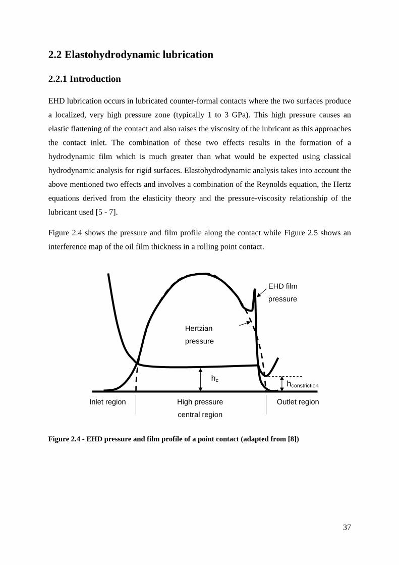
Figure 2.4 shows the pressure and film profile along the contact while Figure 2.5 shows an

interference map of the oil film thickness in a rolling point contact.

Hertzian

pressure

hc

EHD film

pressure

hconstriction

Inlet region High pressure

central region

Outlet region

Figure 2.4 - EHD pressure and film profile of a point contact (adapted from [8])

Figure 2.5 - Interference map of an EHD point contact. The central flat region is of almost

uniform thickness, hc, while the side lobes are arou

At the inlet, the build-up of the fluid pressure occurs and the lubricant is entrained by the

moving surfaces into the central high pressure zone. The pressure distribution and film

profiles in this region are predetermined by the elastic

this region is sometimes referred to as the Hertzian region. The film returns to ambient

pressure in the outlet region.

The profile obtained in an EHD contact can be explained by considering the Reynolds

equation which is obeyed by the lubricant in the contact [

NNO PQR

SNTNO

As the lubricant enters the contact, the pressure

viscosity, ., increases by several orders of magnitude (see Section

finite and decrease towards the centre of the contact, as determined by the Hertz equations

which describe the elliptical pressure distribution within the

from Equation 2.1, as the viscosity of the lubricant increases enormously,

a very low value, hence the film variation becomes

a flat film profile in the central region (see Figure

at the inlet determines the film in the central region,

central region and the viscosity becomes very high, the film thickness

In the exit region, the lubricant must return to ambient pressure. A very rapid drop in the

pressure and, consequently, an even bigger drop in the viscosity occurs, both of which boost

the flow outwards very fast. In order to avoid continuity of flow pr

inlet

of an EHD point contact. The central flat region is of almost

while the side lobes are around 0.75 hc (hmin)

up of the fluid pressure occurs and the lubricant is entrained by the


profiles in this region are predetermined by the elastic deformation of the boundaries. In fact,


he profile obtained in an EHD contact can be explained by considering the Reynolds

hich is obeyed by the lubricant in the contact [7]:

NTNOU � N

NV PQRS

NTNVU � WXY ZQ

ZO

As the lubricant enters the contact, the pressure, p, increases and, as a result of this, the

increases by several orders of magnitude (see Section 2.2.1.


which describe the elliptical pressure distribution within the contact (see Figure 2.4

, as the viscosity of the lubricant increases enormously, ��4

hence the film variation becomes very small in the x-direction, resulting in

the central region (see Figure 2.4). This also means that the film formed

the film in the central region, hc, as, once the pressure increases in the

central region and the viscosity becomes very high, the film thickness does not var



the flow outwards very fast. In order to avoid continuity of flow problems, a constriction

38

of an EHD point contact. The central flat region is of almost

up of the fluid pressure occurs and the lubricant is entrained by the


deformation of the boundaries. In fact,


he profile obtained in an EHD contact can be explained by considering the Reynolds

Equation 2.1

increases and, as a result of this, the

2.2.1.2). [\[4 and

[\[� are


Figure 2.4). As seen

�$�4 must decrease to

direction, resulting in

). This also means that the film formed

as, once the pressure increases in the

oes not vary.



oblems, a constriction

39

occurs at the inlet. The separation decreases at the end of the contact, with the film thickness

reducing by about 25% (hmin) and continuity of flow is maintained. The constriction extends

around the side of the contact, forming a ‘horse-shoe’ shaped constraint [9], as seen in Figure

2.5, with the minimum film thickness, hmin, usually occurring at the ‘side-lobes’. The pressure

spike seen in Figure 2.4 is associated with the constriction formed at the end of the contact.

The pressure spike increases with increasing speed and the constriction occupies a broader

part of the Hertzian contact region [6]. Thus, as the entrainment speed increases, the shape of

the film changes.

2.2.1.1 Regimes in fluid film lubrication

The above description is only valid when the lubricated counter-formal contact operates in

true EHD conditions (i.e. both elastic deformation and an increase in viscosity with pressure

occur at the contact). There are, in fact, four possible types of contact operating conditions as

illustrated by the chart in Figure 2.6.

Figure 2.6 - Chart showing the four possible types of operating conditions for circular contacts

in full fluid film lubrication [10]. Similar charts are available for line and elliptical contacts.

40

• Isoviscous-elastic

This type of lubrication occurs either when one of the containing surfaces has a low

elastic modulus, such as rubber or human tissue, or, in the case of stiffer materials,

when the lubricant has a very low pressure-viscosity coefficient. An example of such

a lubricant is water.

• Piezoviscous-elastic

This type of lubrication occurs in most steel/ceramic counter-formal contacts, where

true EHD behaviour is exhibited.

• Isoviscous-rigid

This operating condition is best described by the classical hydrodynamic lubrication

theory and occurs only at low contact pressures and very low loads.

• Piezoviscous-rigid

This type of lubrication occurs at low loads with oils having a high pressure-viscosity

coefficient, or with normal loads and very inelastic solids.

These charts can be easily constructed for both point and line contacts using a number of

equations (which are a function of the operating conditions) which define the boundaries

between the four operating conditions. All the detailed equations can be found in [8]. The

two dimensionless parameters used in the chart for point contacts, gv and gE, give the

significance of variation in viscosity within the contact and the ratio of the pressure generated

in the film to the pressure in the underlying substrate respectively and are given by:

]^ � _;666RY;X Equation 2.2

]a � 666b R⁄Y;X Equation 2.3

The terms used in Equations 2.2 and 2.3 are defined in Nomenclature. These two parameters

therefore determine the type of operating condition in which a contact operates.

Different regression equations which give the thickness of the film formed are available for

each contact condition. In this work, two of the four types of contact conditions were

covered. The oil-lubricated contacts investigated in this study operate in true EHD conditions

and are piezoviscous-elastic while the water-lubricated contacts are isoviscous-elastic. The

corresponding film thickness equations for each type of contact are given in Sections

2.2.2.1.1.1 and 2.2.2.1.2.1.

41

2.2.1.2 Effect of pressure and temperature on viscosity

Viscosity is a very important rheological property as it plays a major role in determining the

thickness of the film formed in an EHD contact. The lubricant is subjected to high pressures

and different temperatures hence it is essential to understand the effect of both pressure and

temperature on the viscosity of the lubricant.

The viscosity of most lubricants greatly increases when subjected to high pressures. The

Barus equation is usually used to describe this behaviour:

S � ScdeT Equation 2.4

where .( is the viscosity at atmospheric pressure and is the pressure-viscosity coefficient.

For most lubricants (oils), lies between 10 and 25 GPa-1 and decreases with increasing

temperature.

The viscosity of oil decreases rapidly with increasing temperature. Many equations which

describe the behaviour of lubricants with temperature exist. One viscosity-temperature

relationship which is very accurate at low temperature is given by Vogel:

S � fdg �h�i�⁄ Equation 2.5

where A, B and C are constants.

For the range of temperatures used in most engineering applications, the ASTM chart is used

to describe the variation of viscosity of the lubricating oils with temperature.

This chart is the basis of the standard provided by the American Society of Testing Materials

(ASTM D341-722) which describes the variation of kinematic viscosity, C (� . E⁄ , jkl),

with temperature, T (in Kelvin), by the empirical equation:

mn] mn]�o � p. r� � g , i mn] h Equation 2.6

By plotting stu stu�C � 0.7� against stu/, a straight line is obtained. Hence, if the viscosity

of the lubricant at two temperatures is known, constants B and C are found, and the viscosity

at any temperature can then be determined.

42

One other relationship worth mentioning is the effect of shear rate on viscosity. When the

viscosity of the lubricant is independent of the shear rate, the lubricant is referred to as

Newtonian. When the viscosity varies with shear rate, the lubricant is non-Newtonian. In

EHD contacts, the lubricant behaves as a Newtonian fluid at the inlet of the contact, however,

inside the contact, the lubricant is non-Newtonian.

43

2.2.2 EHD film forming and friction properties of lubric ants

EHD film thickness is determined by the quantity of the lubricant entrained into the contact

and is therefore dependent on the rheological properties of the lubricant under the conditions

of the contact inlet, while EHD friction originates within the central region of the contact and

is determined by the rheological response of the lubricant to the very high pressure and shear

rate present [11]. The corresponding properties for single-phase (neat oil and pure water) and

two-phase (oil-in-water emulsion) lubrication are given in this section.

2.2.2.1 Single-phase lubrication

2.2.2.1.1 EHD film forming and friction properties of neat oil

2.2.2.1.1.1 EHD film formation

Over the past 60 years, the thickness of the film of lubricant formed in EHL contacts has been

widely investigated and is now well understood. Regression equations based upon numerical

analysis of fully flooded, isothermal conditions are commonly used to estimate the film

thickness. These equations are generally expressed in terms of three main non-dimensional

groups known as the speed (1;), load (<; ) and material (��) parameters (terms are defined in

Nomenclature).

The most widely used equations to predict isothermal elastohydrodynamic film thickness in

hard EHL elliptical contacts are by Dowson and Hamrock [12,13], where the central, hc , and

minimum, hmin, film thickness for elliptical contacts are given by:

Qx yzn � X. {|Y;p.{r_;p.}R666�p.p{r�W , p. {Wd�p.r}~� V � O⁄ �p.{�� O Equation 2.7

Q�� yzn � R. {RY;p.{b_;p.�|666�p.prR�W , d�p.rp~� V � O⁄ �p.{�� O Equation 2.8

Equations 2.7 and 2.8 apply to elliptical contacts and are used to predict film thickness in this

study (see Chapter 4). The cold rolling process however usually involves line contacts.

Equations 2.9 and 2.10 give film thickness for line contacts.

Qx yzn � R. WWY;p.{|_;p.}{666�,p.W� O Equation 2.9

Q�� yzn � X. {}Y;p.r_;p.}�666��p.WR� O Equation 2.10

44

Equation 2.7 implies that, as long as the contact remains in the piezoviscous-elastic regime, a

plot of the logarithm of the central film thickness against that of speed gives a straight line,

with a slope of 0.67. This equation is used successfully to predict film thickness and has been

validated experimentally up to a speed of around 5 m s-1. Very little experimental data is

available at higher speeds.

2.2.2.1.1.1.1 Factors affecting film thickness at high speeds

The speed parameter plays a major role in determining the film thickness. As the speed is

increased, more lubricant is entrained into the contact and, as a result of this, a thicker film is

formed. At high entrainment speeds (usually above 5 m s-1), other factors start influencing

film thickness behaviour, and film thickness values obtained experimentally start to deviate

from those predicted by Equation 2.7 [14].

Two factors which may contribute to this reduction in film thickness below the values

predicted by the isothermal regression equations are starvation and thermal effects.

Starvation

Starvation occurs when the speed becomes so high that the rate of formation of the pool of

lubricant in the inlet region becomes insufficient to balance the rate at which it passes

through and around the contact. As a result of this, the film thickness falls with a further

increase in speed. The fundamental parameters which influence the rate of replenishment of

the oil pool are surface tension effects in the vicinity of the contact, the base oil viscosity, the

amount of lubricant present on track, the track width and the velocity [15]. Once the contact

is in the starved regime, the film thickness starts decreasing with increasing speed [Figure

2.7].

There is no straightforward way of predicting the onset of starvation, as a description of

factors influencing the rate of supply of the fluid to the inlet region is required and many of

these are not easy to estimate, examples being the surface film thickness or the inlet meniscus

distance. However, if one surface is transparent, optical microscopy of the inlet region

provides a simple and effective way to determine if the contact is starved. For mildly starved

contacts, the inlet meniscus may be observed in front of the contact, while for heavily starved

contacts, the meniscus coincides with the Hertzian contact circle (Figure 2.7) [16].

45

Figure 2.7 - Typical EHL film thickness against speed curves for the fully flooded and starved

regimes. Optical interferometry pictures depicting a fully flooded and starved contact are also

shown (inlet is on the right) [16].

The inlet meniscus distance defines whether a fully flooded or a starved condition exists in

the contact. The critical inlet meniscus, which is defined as the distance below which

starvation occurs, is given by the dimensionless value, m*, where:

�� W � R. p{ ��O� �X ��,��p.}b

Equation 2.11

where HC,F is the dimensionless central film thickness for fully flooded conditions given by

�' �7( 3 4⁄ . A fully flooded condition exists when the inlet meniscus, m > m*, and a starved

condition exists when m < m* [17].

Shear thinning

Shear thinning could also affect film thickness at high speeds. If the lubricant is non-

Newtonian, at high speeds and therefore high shear rates, the viscosity of the lubricant will

drop significantly with increasing speed, resulting in a lower film thickness than that

predicted by classical Newtonian equations such as the Dowson-Hamrock equation. At very

high shear rates, usually greater than 109 s-1, all fluids probably shear thin, however, in most

low pressure, hydrodynamic lubricated contacts, shear rates do not exceed 107 s-1, therefore,

in such conditions, lubricants are unlikely to shear thin.

46

Thermal effects

Thermal effects can also play a major role in determining the film thickness at high speeds

since a rise in temperature in the inlet region reduces the local viscosity and leads to a lower

film thickness. The extent of the temperature rise is determined by the degree of shearing

present and on the temperature-viscosity behaviour of the lubricating fluid. Thermal effects at

high speeds have been reported by several workers [14,18].

Thermal reduction of film thickness in elastohydrodynamic lubrication may arise from inlet

shear heating, even in pure rolling. However, the effect is further exacerbated by the presence

of sliding [9].

Thermal correction factors are commonly used to correct for these effects. The isothermal

film thickness, hiso, is modified by a thermal reduction factor, CT, to estimate the correct

value of film thickness under the prescribed operating conditions. Many thermal correction

factors are available [19-22] however, until now, none of these has been validated

experimentally at very high speeds.

The thermal reduction factor which will be used in this analysis is the one proposed by Gupta

et al. [22] which is given by:

ih � W�WR.XTca �p.�XW5p.XWR~W5X.XR�p.bR��p.{� Equation 2.12

where the loading parameter, L, is defined by:

� � , �NSNh� YX

� Equation 2.13

and the slide-roll ratio, S:

� � X YW�YXYW5YX Equation 2.14

This correction factor is an improved version of that due to Wilson and Sheu [19]. It

combines Wilson and Sheu’s analysis which also incorporated the effect of inlet shear

heating due to sliding with the ‘load effect’ calculated by Cheng [20]. The predicted film

thickness taking into account thermal effects is obtained by multiplying the isothermal film

thickness with the thermal reduction factor (h = hiso × CT).

47

In addition to its effect on the inlet region, sliding also causes frictional dissipation

throughout the contact, which may appreciably increase the bulk temperature of the surfaces

above ambient. This is not accounted for by inlet shear heating corrections but can become

significant if both high loads and sliding speeds are present, an example being in the

lubrication of gear teeth [3].

Both thermal effects and starvation are highly dependent on speed and both can be

experienced at high speeds. Thus, for high speed applications such as metal forming and

high-speed bearings, which may operate at speeds as high as 20 m s-1, these factors must be

taken into account. Very little experimental data is available for film thicknesses at speeds

above 5 m s-1. The only work found was by Dickenson in 1982, when correction factors were

still at their early stages [14].

48

2.2.2.1.1.2 EHD friction

The friction of an EHD contact is the integral of the shear stress, τ, developed in the lubricant

film over the contact area and is determined by the rheological response of the lubricant to

the very high pressure and shear rate present. In the fluid film lubrication regime, traction is

due to shearing of the lubricant in the contact (sliding friction) and shearing of the lubricant

in the inlet and outlet zone (rolling friction).

Rolling friction

In pure rolling, even if there is no nominal fluid shear in the contact, a small retarding action

force is present. This traction originates in the contact inlet, possibly due to the shearing of

the lubricant within this zone [23]. In sliding-rolling contacts, rolling friction is usually

ignored, as its contribution compared to that of sliding friction is found to be slight [9].

Sliding friction

Sliding friction originates within the central region (parallel film high pressure region) of the

contact. Upon entering the conjunction, if there is externally applied sliding or spin between

the surfaces, the resulting friction which opposes this motion is governed by the shear

properties there [9]. Traction therefore depends on the properties of the lubricant in the centre

of the EHD contact, where very high pressures and shear rates are experienced.

When considering sliding contacts, the mean properties of the film across the contact are

usually used to determine friction. The friction coefficient is then given as:

� � �` � � �Zf

� TZf � �6fT;f � �6

T; Equation 2.15

where G� is the mean shear stress and ?� is the mean contact pressure.

Another assumption that is usually made is that all of the friction originates from Couette

flow within this region. The mean strain rate, BA , is then given as:

�A � ∆YQ� Equation 2.16

One important aspect to keep in mind when considering EHD friction is that, whereas the

lubricant behaves as a Newtonian fluid at the inlet of the contact, where the film formed in

the parallel part of the contact is determined (by the entry viscosity), the lubricant inside the

49

contact is non-Newtonian. This is because the shear stress in the contact is very high. Very

high shear rates are required to produce the high strain rates required to slide the layers of

highly viscous lubricant layers of molecules past one another. Once high shear rates are

reached, the lubricant starts to shear thin, and the viscosity decreases with increased shearing.

Rheological models such as those by Johnson et al. [24] which describe the behaviour of

lubricants in EHD contact conditions have been developed. These describe friction as a

function of sliding as follows:

At a very small amount of sliding, the fluid is Newtonian. Friction increases linearly with

increasing sliding and the shear stress is given by:

� � S�A � ScdeT; ��Q� Equation 2.17

At a significant sliding speed and strain rate, the shear stress becomes very high as a result of

the high pressure at the contact which causes the viscosity to rise. This will cause shear

thinning, and the viscosity decreases with increasing shear rate. At this point there are

therefore two effects opposing each other. The increased shearing resulting from increased

strain rate which results from increased sliding and a lower film thickness (film thickness

reduces due to shear thinning) will be opposed by the effect of shear thinning which lowers

the viscosity therefore reducing the shear stress. This behaviour can be described by the

following equation:

�6 � �d ��W �S�A�d � � �d ��W PScdeT;�Y

�x�d U Equation 2.18

where G�, the Eyring stress, is a characteristic stress at which shear thinning starts to occur.

At very high shear rates (or very high pressures), the fluid yields at the limiting shear

stress,G=. EHD friction will then depend on the yield strength of the very high pressure non-

Newtonian film. Once the limiting shear stress is reached, the traction coefficient becomes

the limiting traction coefficient,G � G=, and remains constant with further increase in sliding.

The limiting traction coefficient depends upon the molecular nature of the lubricant and

increases linearly with pressure and also decreases linearly with temperature. For most

mineral oils, the limiting traction coefficient at room temperature is between 0.05-0.07 and

50

decreases to around 0.03 to 0.05 at 100˚C whereas synthetic ester oils have even lower

limiting traction coefficients [25].

In most cases it can be assumed that contact pressure is high enough for thin films to reach

the limiting shear stress and limiting coefficient of friction. Figure 2.8 shows this behaviour

where it can be seen that the limiting shear stress is reached in the EHD regime and the

friction coefficient remains constant with increasing sliding (and entrainment speed) and then

drops slightly due to thermal effects which lower the limiting friction coefficient.

Figure 2.8 - Variation of coefficient of friction with speed and viscosity [26]

2.2.2.1.1.2.1 Factors affecting friction at high speed

Unlike film thickness, which depends on the entrainment speed, sliding friction is dependent

on the amount of sliding, �Δ1�, and to some extent is independent on the entrainment speed.

However, at very high entrainment speeds, factors not present at low speed may occur.

Possible factors include shear heating and viscoelastic response [11], both of which result in a

reduction in friction. To date, no experimental work on friction behaviour of neat oil at very

high entrainment speeds is available.

thermal effect

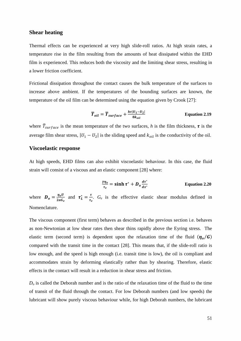
51

Shear heating

Thermal effects can be experienced at very high slide-roll ratios. At high strain rates, a

temperature rise in the film resulting from the amounts of heat dissipated within the EHD

film is experienced. This reduces both the viscosity and the limiting shear stress, resulting in

a lower friction coefficient.

Frictional dissipation throughout the contact causes the bulk temperature of the surfaces to

increase above ambient. If the temperatures of the bounding surfaces are known, the

temperature of the oil film can be determined using the equation given by Crook [27]:

h;nym � h;z�� d � Q�|YW�YX|b�nym Equation 2.19

where /6789:�'� is the mean temperature of the two surfaces, h is the film thickness, � is the

average film shear stress, |1� , 1�| is the sliding speed and 2(�� is the conductivity of the oil.

Viscoelastic response

At high speeds, EHD films can also exhibit viscoelastic behaviour. In this case, the fluid

strain will consist of a viscous and an elastic component [28] where:

�A Sc�d � �� ¢c Z��

ZO� Equation 2.20

where ¢c � ScYX _d and ��

�d. Ge is the effective elastic shear modulus defined in

Nomenclature.

The viscous component (first term) behaves as described in the previous section i.e. behaves

as non-Newtonian at low shear rates then shear thins rapidly above the Eyring stress. The

elastic term (second term) is dependent upon the relaxation time of the fluid �Sc _⁄ �

compared with the transit time in the contact [28]. This means that, if the slide-roll ratio is

low enough, and the speed is high enough (i.e. transit time is low), the oil is compliant and

accommodates strain by deforming elastically rather than by shearing. Therefore, elastic

effects in the contact will result in a reduction in shear stress and friction.

Do is called the Deborah number and is the ratio of the relaxation time of the fluid to the time

of transit of the fluid through the contact. For low Deborah numbers (and low speeds) the

lubricant will show purely viscous behaviour while, for high Deborah numbers, the lubricant

52

will show viscoelastic effects [9]. Do is a function of the entrainment speed, U, therefore, the

higher the entrainment speed, the more likely it is for the lubricant to show viscoelastic

behaviour, with the elastic term becoming more significant with increasing speed.

2.2.2.1.2 Film formation and friction properties of water

2.2.2.1.2.1 Film thickness

Water has a low viscosity (0.00066 Pa s) and, more importantly, a very low pressure-

viscosity coefficient. Whereas typical mineral oils have a pressure-viscosity coefficient in the

range of 10-22 GPa-1, the value of water has been reported to be 0.36 GPa-1 at 50°C [29, 30].

Experimental work has shown that measured film thickness for water is much higher than

that predicted by EHD film thickness equations such as Equation 2.7 [30]. This is because

water has such a low pressure-viscosity coefficient that the contact acts in the isoviscous-

elastic regime rather than in the conventional piezoviscous-elastic regime. EHD film

thickness equations such as those given by Equation 2.7 and Equation 2.8 become applicable

only when there is a significant increase in viscosity at the inlet, which is not the case for

water, therefore other equations must be used. Central film thickness for fluids operating in

the isoviscous-elastic regime can be predicted by the equation given by Hooke [31] for point

contacts:

Q� � �. Wb YSp.{� p.{ra p.�r`p.WR Equation 2.21

This equation has been successfully validated and proved to give very good agreement with

experimental results [30]. When predicting film thickness for elliptical contacts, the equation

given by Dowson and Hamrock [32] for the isoviscous-elastic regime is used in this study,

where:

Q� � r. RXY;p.{�666�p.XX�W , p. rXd�p.X|~�V£ �O£⁄ �p.{��¤O Equation 2.22

53

2.2.2.1.2.2 Friction

In piezoviscous-elastic EHL contacts, very high pressures and shear rates are present in

sliding EHL contacts. However, this is not the case in isoviscous-elastic conditions. This is

because the pressure-viscosity coefficient of water is very low, hence the increase in viscosity

due to pressure is negligible at the contact.

One common approach in predicting friction of water is to assume that only Couette shear

takes place. In this case, Equation 2.17 can be used to determine the shear stress, from which

the traction coefficient can then be deduced:

� � �6T; � ∆�ScdeT;

T;Q� Equation 2.23

Experimental results however have shown that this approximate approach does not accurately

predict traction coefficient and that, for isoviscous-elastic conditions, rolling friction is not

negligible [33]. A fuller approach is required, where the shear stress is defined as:

� � ¥ ��SQx , QNT

X¦O Equation 2.24

where the first term is due to Couette flow (sliding friction) and the second, pressure

gradient-dependent term, results from Poiseuille flow (rolling friction).

Friction increases linearly with increasing sliding and shear stress and, due to the very low

viscosity of water at the contact, is much lower than the values obtained for oil. The

measured friction values for water reported by various researchers are much lower than those

obtained for oil and fall below 0.01[33].

54

2.2.2.2 Two-phase lubrication

2.2.2.2.1 Introduction

An emulsion is a type of colloid which is defined by Becher [34] as ‘a heterogenous system,

consisting of at least one immiscible liquid intimately dispersed in another in the form of

droplets, whose diameters, in general, exceed 0.1 µm’.

Oil-in-water emulsions are two–phase liquid systems which consist of oil uniformly

dispersed in water. To disperse the oil into the water phase, an emulsifier (also referred to as

surfactant) is required. Emulsifiers contain a hydrophilic moiety which attracts water and a

lipophilic moiety which attracts oil, thereby promoting the formation of a stable emulsion of

oil and water by inhibiting the close approach of one droplet to another. The polar

(hydrophilic) part of the molecule can also carry a positive or negative charge and therefore

emulsifiers can be classified into non-ionic, cationic and anionic surfactants. Emulsifiers with

a high Hydrophile-Lipophile Balance (HLB) number, which is a measure of the relative

percentage of hydrophilic to lipophilic groups in the surfactant molecules [35], are used to

stabilize oil-in-water emulsions (number typically ranges from 8 to 18, [36]). The selection of

emulsifiers is still made on empirical basis.

The diameter of the oil droplets in an oil-in-water emulsion typically lies between 0.1 �m and

0.1 mm. A range of droplet sizes is usually present in an emulsion. The particle size

distribution can be broad or wide, with the narrow distribution being described as one where

the ratio between smallest and largest droplet size is 0.1. The droplet size depends on many

factors including the emulsifier type (including the HLB number) and concentration, water

hardness, temperature and mixing time [37]. The droplet size increases with time due to

separation effects, the extent of which is dependent on the stability of the emulsion.

The stability of emulsions depends on many factors such as the emulsifier type and

concentration, droplet size, solubility of the oil in the aqueous phase, oil type and

concentration, pH, the activity present at the surface and interfaces (which affects the

adsorption of the emulsifier) and the temperature at which emulsification is carried out. These

factors all affect the break-down of the emulsion which can occur by various processes such

as sedimentation (or creaming), flocculation and coalescence. Measuring the variation in the

55

mean droplet size as well as the % volume of the separated oil phase with time gives an

indication of the stability of emulsions.

The viscosity of an oil-in-water emulsion depends on the viscosities of the two phases and the

phase volume as well as other properties such as the droplet size and distribution as well as

emulsifier type and concentration.

For dilute emulsions (< 5% oil), the viscosity can be calculated using the equation given by

Einstein [38] where:

S � �W � X. }I�S� (Einstein) Equation 2.25

where .c, is the viscosity of the continuous phase and ¨ is the concentration of the

discontinuous phase.

For more concentrated emulsions, improved relationships which take into account the

presence of neighbouring droplets are given by Sibree [39] and Eilers [40] where:

S � S�W� ©W.RIR (Sibree) Equation 2.26

S � ªW � W5X.}IX�W�W.R}I�«

X S� (Eilers) Equation 2.27

All the above relationships assume that the oil droplets are rigid. This is probably a valid

assumption for oil-in-water emulsions which are entrained within the contact, where the

viscosity of the oil droplets is extremely high. As the emulsion concentration increases

further, oil-in-water emulsions may invert to water-in-oil emulsions.

In this study, a commercial oil which already contains an emulsifier (emulsifiable oil) is used

hence the same emulsifier type and concentration as well as the same method of preparation

were used for all oil-in-water emulsion investigated. The major focus was given to dilute

emulsions since the latter reflect the concentrations used in cold rolling. Dilute oil in-water

emulsions are also widely used as fire resistant hydraulic fluids in high fire risk applications

such as in mining [41,42].

56

2.2.2.2.2 Film forming and friction properties for oil-in-wa ter emulsions

2.2.2.2.2.1 Mechanisms of film formation of oil-in-water emulsions

There has been considerable research carried out to study the elastohydrodynamic film

forming properties of oil-in-water emulsions [42-46]. In recent years most of this has been

based on optical interferometry, (and since 1994 ultra-thin film interferometry), which is able

to measure film thickness directly within the contact formed by a steel ball or roller and a

transparent flat [47-52].

Oil-in-water emulsions show a complex pattern of behaviour, which can be explained in three

stages as illustrated schematically in Figure 2.9.

At slow speeds, (Stage I), a well-designed oil-in-water emulsion forms a small pool of oil

phase in the contact inlet. To do this, the oil phase must preferentially wet the metal surface

and this can be controlled by appropriate choice of emulsion properties such as emulsifier

type, emulsifier concentration, base oil type and pH (which affects the stability of an

emulsion). The existence of this oil pool means that the elastohydrodynamic film thickness

has the same value as that formed by neat oil and increases with increasing speed according

to the classical relationship h ∝ U0.7 where U is the mean rolling speed. The film thickness of

oil-in-water emulsions at slow speeds can therefore be predicted using film thickness

equations such as those given by Dowson and Hamrock (Equation 2.7).

base fluid

oil in water emulsion

log(mean rolling speed)

log(

film

thic

knes

s)

Stage 1 Stage 2 Stage 3

base fluid

oil in water emulsion

log(mean rolling speed)

log(

film

thic

knes

s)

Stage 1 Stage 2 Stage 3

h ∝ U0.7

Stage I Stage II Stage III

oil-in-water

emulsion

Figure 2.9 - Behaviour of oil-in-water emulsions with speed (adapted from [48])

base oil

57

Figure 2.10 - Picture illustrating phase inversion which occurs at the inlet of the contact in Stage

I [48]

At some critical speed however, the rate of pool formation becomes insufficient to balance

the rate at which it passes through and around the contact. At this point, EHD starvation

ensues, and the film thickness falls, often quite sharply, with increase in speed (Stage II) [47].

The speed at which Stage II initiates (first critical speed) depends on the composition and

chemical properties of the emulsion.

Usually the film thickness does not fall to zero, however, and at a still higher rolling speed

(second critical speed), typically between 1 and 4 m s-1, it starts to rise again and Stage III

behaviour ensues [48]. This region has been relatively little studied but it has been suggested

that, under these conditions, a mixture of oil and water [46, 48] or a dynamic concentration of

oil droplets [53] could be entrained into the contact. The second critical speed also depends

on the composition and chemical properties of the emulsion.

One important aspect which has not yet been investigated is what is actually entrained inside

the contact beyond the second critical speed. Knowledge of the composition of the entrained

lubricant would enable a better understanding of the lubrication mechanism occurring at high

speed. Direct observations of the emulsion flow in the inlet region have been done up to a

speed of 1.5 m s-1 [46, 48, 54] however Stage III was not covered. No work has yet been done

to investigate the composition of the entrained lubricant at high speeds.

Recently a model has been developed for EHD emulsions which covers all three stages of

behaviour of emulsions [55]. This model however still does not fully take into account all the

emulsion characteristics (a unique factor is used to take into account the combined effects

from the emulsifier, pH value, droplet size etc) and more experimental results at high speeds

are required to validate it and ensure that the assumption used to describe the emulsions

behaviour in Stage III (a mixture of oil and water is entrained) is mechanistically correct.

58

2.2.2.2.2.1.1 Behaviour of oil-in-water emulsions at low speed

Stage I

Most of the previous work done on oil-in-water emulsions has focused on slow speed

behaviour and thus on Stage I as indicated in Figure 2.9. As a result, the slow speed

behaviour of oil-in-water emulsions is now quite well understood and, based on this

understanding, guidelines for the design of effective oil-in-water emulsions have been

produced.

At low speeds, the main lubricating mechanism is plate-out. The oil droplets are adsorbed

into the metal surface and spread to an angle which is known as the wetting angle. A film of

oil is plated out on the surface, causing a pool of oil to form in the inlet region of the counter-

formal contact. Direct observations by Nakahara et al. [46], Zhu et al. [48] and Yang et al.

[54] confirmed the existence of an oil-rich pool in the inlet region at low speeds (phase

inversion region, Figure 2.10) for both point and line contacts. As long as the emulsion is

able to form a pool of oil at the inlet whose size is greater than the critical inlet meniscus, the

emulsion behaves similarly to neat oil in fully flooded conditions and the film formed is

highly dependent on the viscometric properties of the oil phase [47].

The ability of the emulsion to wet the surface is highly dependent on the emulsifier

concentration. Extensive work has been carried out by various researchers on the effect of

emulsifier concentration on the film forming properties of emulsions in Stage I [43, 44, 46,

49, 50, 52]. Nakahara et al. [46] observed that a high emulsifier concentration prevents the

occurrence of phase inversion in the low rolling speed region and markedly reduces the film

thickness. Using a displacement energy approach which was first suggested by Kimura and

Okada [44], Ratoi-Salagean et al. [50] showed that the wetting properties of emulsions are

well described in terms of the critical micelle concentration, cmc, of the emulsifier, which is

the concentration at which the adsorbed layer of surfactant is thicker than a monolayer (full

monolayer coverage is obtained at a lower concentration, Ca) and the surface tension of the

emulsifier solution in water levels out (see Figure 2.11). When a complete monolayer of

surfactant is present, the surface is highly hydrophobic (due to the orientation of the

surfactant molecules) however, as the emulsifier increases, a second layer of surfactant

forms. The orientation of the polar heads in the second layer is inverted and the surface then

becomes hydrophilic. Thus, when the emulsifier concentration is higher than the critical

59

micelle concentration, the emulsion shows poor wettability whereas, if the emulsion

concentration is lower than the critical micelle concentration, the emulsion shows good

wettability and the film formed is sustained for a relatively wide range of speed (typically up

to about 0.1-0.5 m s-1) and is very close to that obtained by the corresponding neat oil [50].

Figure 2.11- Plots showing (a) the variation of oil/solid, θos, and water/solid θws, contact angles

and (b) the variation of the two liquid/air surface tension, γOA γWA, with emulsifier

concentration. The location of the critical micelle concentration as well as an illustration of the

variation in the adsorbed layer with emulsifier concentration are also displayed (from [50]).

Ratoi-Salagean et al. [50] and Cambiella et al. [52] showed that emulsion concentration is the

key characteristic in determining the film forming properties of emulsion in Stage I and,

although some of them affect interfacial properties such as contact angle and interfacial

tension, other factors, such as droplet size, oil concentration, stability and emulsion viscosity

play a minor role in the film formation of emulsions at low speeds. When the emulsifier

concentration is at a constant concentration at which the emulsion is able to form a pool by

plate-out (as is the case for this study) variations in film thickness are then dependent on the

ability of the emulsion to maintain this pool and factors such as speed, droplet size, stability

and oil concentration play a key role in determining the thickness of the film formed.

The size of the pool of oil is highly influenced by the speed. For emulsions to form films of

similar thickness as their corresponding oil, the rate of oil pool formation at the inlet must be

sufficient to replenish the oil which goes through and around the contact, thereby maintaining

an oil pool bigger than the critical inlet distance. As the speed increases, less time is available

for the pool to form, and, as a result of this, the oil pool decreases with increasing speed. This

behaviour has been confirmed by direct observations of the inlet by various researchers (46-

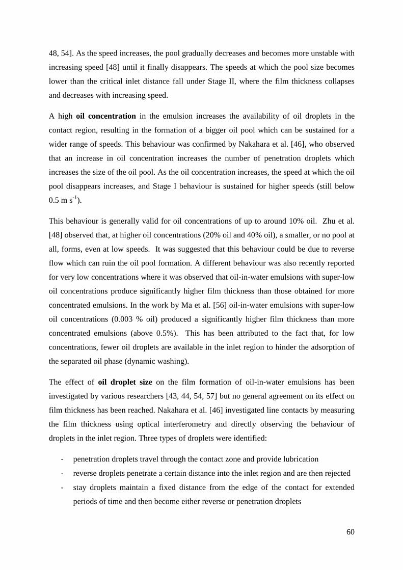
60

48, 54]. As the speed increases, the pool gradually decreases and becomes more unstable with

increasing speed [48] until it finally disappears. The speeds at which the pool size becomes

lower than the critical inlet distance fall under Stage II, where the film thickness collapses

and decreases with increasing speed.

A high oil concentration in the emulsion increases the availability of oil droplets in the

contact region, resulting in the formation of a bigger oil pool which can be sustained for a

wider range of speeds. This behaviour was confirmed by Nakahara et al. [46], who observed

that an increase in oil concentration increases the number of penetration droplets which

increases the size of the oil pool. As the oil concentration increases, the speed at which the oil

pool disappears increases, and Stage I behaviour is sustained for higher speeds (still below

0.5 m s-1).

This behaviour is generally valid for oil concentrations of up to around 10% oil. Zhu et al.

[48] observed that, at higher oil concentrations (20% oil and 40% oil), a smaller, or no pool at

all, forms, even at low speeds. It was suggested that this behaviour could be due to reverse

flow which can ruin the oil pool formation. A different behaviour was also recently reported

for very low concentrations where it was observed that oil-in-water emulsions with super-low

oil concentrations produce significantly higher film thickness than those obtained for more

concentrated emulsions. In the work by Ma et al. [56] oil-in-water emulsions with super-low

oil concentrations (0.003 % oil) produced a significantly higher film thickness than more

concentrated emulsions (above 0.5%). This has been attributed to the fact that, for low

concentrations, fewer oil droplets are available in the inlet region to hinder the adsorption of

the separated oil phase (dynamic washing).

The effect of oil droplet size on the film formation of oil-in-water emulsions has been

investigated by various researchers [43, 44, 54, 57] but no general agreement on its effect on

film thickness has been reached. Nakahara et al. [46] investigated line contacts by measuring

the film thickness using optical interferometry and directly observing the behaviour of

droplets in the inlet region. Three types of droplets were identified:

- penetration droplets travel through the contact zone and provide lubrication

- reverse droplets penetrate a certain distance into the inlet region and are then rejected

- stay droplets maintain a fixed distance from the edge of the contact for extended

periods of time and then become either reverse or penetration droplets

61

The larger droplets in the emulsion are generally penetration droplets while smaller ones are

reverse droplets. They also observed that the large penetration droplets reduce in number as

the speed increases; the stay droplets locate further from the contact at higher speed; and the

small reverse droplets do not vary with speed.

Most of the observations by Nakahara et al. [46] were carried out at very low speeds (0.005-

0.02 m s-1). Direct observations of the inlet region were also carried out by Yang et al. [54]

and Zhu et al. [48] using both point and line (highly elliptical) contacts and covering a wider

range of speeds (up to 1.5 m s-1). Similar oil droplet behaviour was observed by both

researchers. Yang et al. [54] confirmed the three types of oil droplets at the inlet but noted

that, ultimately, the oil droplets that penetrate the contact zone are those primarily attached to

the surfaces or that join the oil pool. Yang et al. also observed that, for both point and line

contacts, the size of oil pool is more sensitive to the droplet size for smaller droplets (below

5�m). When compared to line contacts, more droplets go round point contacts as side flow.

This results in the oil pool at the inlet being much smaller in a point contact than in a line

contact under the same conditions [48, 54].

The effect of the stability of an emulsion on pool formation has been investigated by Zhu et

al. [48]. The stability was varied by varying the pH (HCl was added to the lubricant) of the

emulsion. It was found that a more destabilized emulsion (lower pH) forms significantly

larger and more stable oil pools, resulting in a higher film thickness.

62

Stage II

The plate-out theory also describes Stage II behaviour of emulsions. The decrease in film

thickness with speed which occurs in this stage has been attributed to starvation [47]. As the

speed increases and reaches the first critical speed, the rate of pool formation becomes

insufficient to replenish the oil which goes through and around the contact and the size of the

pool of plated out oil at the inlet becomes smaller than the critical inlet meniscus. Both Zhu et

al. [48] and Yang et al. [54] have reported that no oil pool was clearly visible in this stage.

Baker et al. [47] have shown that, in Stage II, the emulsions show similar behaviour to the

corresponding base oil in starved conditions. Starvation equations such as those given in

Chiu’s analysis on neat oil in starved conditions [58] can then be used to describe the films

formed by emulsions at this stage. Chiu’s replenishment theory has shown good agreement

with selected results of Zhu et al. [48] (Figure 2.12).

Figure 2.12- Comparison of Chiu’s replenishment model with selected point contacts by Zhu et

al. [48] A comparison of the dynamic concentration with the high speed results is also shown.

Zhu et al. [48] also suggested that the decrease in thickness in this stage, which is also

referred to as the transition region, could also be partly due to changes in the oil

concentration at the inlet which decreases with speed. In comparison to Stage I, Stage II

behaviour has been less investigated as, in most cases, the main objective of research was to

optimize emulsion properties by maximizing the wetting ability of the oil droplets so that the

first critical speed is pushed to higher speeds and Stage II is avoided.

2.2.2.2.2.1.2 Behaviour of oil

Only one study [48] has measured the beh

where Stage III behaviour is prevalent. The main reason for this deficiency is almost

certainly that most commercial optical interferometry test equipment is limited to a maximum

speed of around 4 m s-1, simply because this is easier to design for and is representative of

most engineering components. However, in terms of studying oil

metal rolling, this is unfortunate since the entrainment speeds in metal rolling are generally

greater than 5 m s-1 and it appears that there is a marked change in emulsion behaviour above

this speed.

Zhu et al. [48] showed that the film

speed increases with speed and

obtained using pure water (Figure 2.

emulsion composition (oil concentration) and stability

employed conventional rather than ultra

the film thicknesses could only be measured up to 50 nm (

‘estimated’ rather than measured

present, one cannot relate emul

rolling speeds.

(a) Figure 2.13 Experimental film thickness results f

the only work carried out at high speeds wit

obtained using conventional interferometry rather than ultra

Behaviour of oil-in-water emulsions at high speed: Stage III

] has measured the behaviour of oil-in-water emulsions above 4 m s



ply because this is easier to design for and is representative of

most engineering components. However, in terms of studying oil-in-water emu

is unfortunate since the entrainment speeds in metal rolling are generally

and it appears that there is a marked change in emulsion behaviour above

showed that the film formed by oil-in-water emulsions after the second critical

speed increases with speed and is lower than that obtained using neat oil but

obtained using pure water (Figure 2.13). The film thickness was also dependent on the

composition (oil concentration) and stability (pH). Unfortunately

employed conventional rather than ultra-thin film optical interferometry, which means that

could only be measured up to 50 nm (films thinner than 50 nm

measured). Also, the study did not measure friction. Consequently

one cannot relate emulsion composition and properties to film forming ability at high

(b) Experimental film thickness results for (a) point and (b) line contacts obtained from

the only work carried out at high speeds with oil-in-water emulsions. These values were

obtained using conventional interferometry rather than ultra-thin interferome

63

water emulsions at high speed: Stage III

water emulsions above 4 m s-1,



ply because this is easier to design for and is representative of

water emulsions for

is unfortunate since the entrainment speeds in metal rolling are generally

and it appears that there is a marked change in emulsion behaviour above

after the second critical

using neat oil but higher than that

also dependent on the

Unfortunately, this study

lm optical interferometry, which means that

thinner than 50 nm were

. Also, the study did not measure friction. Consequently, at

sion composition and properties to film forming ability at high

or (a) point and (b) line contacts obtained from

water emulsions. These values were

thin interferometry [48]

64

There have been two main suggestions as to how emulsions may be entrained at very high

speed (Stage III).

Micro-emulsion theory

Nakahara et al. [46] were the first to directly observe that, at relatively high speed (around

0.8 m s-1), no phase inversion occurs at the inlet and only fine oil droplets enter the EHL

region, probably without causing phase inversion, suggesting that a fine oil-in-water

emulsion is entrained in the contact. Zhu et al. [48] agreed with this when discussing their

experimental film thickness results which covered speeds of up to 20 m s-1, suggesting that

the concentration at the inlet zone becomes close to that of the bulk emulsions and a mixture

of oil and water, possibly in the form of a micro-emulsion, is entrained in the contact (Figure

2.14).

Figure 2.14- Picture illustrating micro-emulsion theory where, at high speeds, a mixture of oil

and water, possibly in the form of a micro-emulsion, is entrained in the contact

If this were the case, effective viscosity relationships (Equations 2.25, 2.26 and 2.27) could in

principle be used to predict film thickness using the isoviscous-elastic film thickness equation

(Equation 2.21).

Dynamic concentration theory

The second theory which attempts to describe Stage III behaviour of emulsions is given by

Wilson et al. [53]. The dynamic concentration theory suggests that, at high speeds, oil

droplets (which are much bigger than the film thickness) are squashed and preferentially

drawn to the contact due to the high viscosity of the oil while the water is squeezed out of the

contact. Hence, even if no extensive pool of oil is present at the contact inlet, mainly oil is

entrained in the contact.

65

Figure 2.15 Picture illustrating dynamic concentration theory (adapted from [53])

The contact is treated as starved, and the film thickness at the inversion (inlet meniscus

position), hi, is described as a function of the droplet size, d, bulk concentration, JK, inlet

concentration, JL (taken as 0.9068, which corresponds to the concentration of a close-packed

cylinders configuration) and an arbitrary entrainment coefficient, C, which is not defined and

can be varied:

Qy � iZ ¬�¬� Equation 2.28

The degree of starvation is determined by the inlet distance hence, by varying C, the

predicted film thickness obtained with this model can be varied.

This theory was compared to Zhu et al.’s experimental work, [48], where good agreement

was achieved by choosing an entrainment coefficient of C = 0.2.

The theory was also compared with a set of results obtained using a two-disc machine [59] ,

where a different value of C (=1/30) was used so as to obtain good agreement. The fact that

the entrainment coefficient is not unique makes it very difficult to asses the validity and

accuracy of this theory by just comparing the theory to film thickness results.

Although this theory is aimed at line contacts, it has been applied by the authors (Wilson et

al. [53]) to point contact results given by Zhu et al. [48] (Figure 2.12), by assuming that the

entrainment coefficient, C, is the same as that applied to the line contact film thickness values

for the same droplet size and concentration.

66

2.2.2.2.2.2 Friction properties of oil-in-water emulsions

Only one work was found to have measured friction at three speeds which fall under all three

stages of behaviour of emulsions [51].

It has been shown that at low speeds, in Stage I, the friction coefficient obtained with oil-in-

water emulsions in mixed sliding/rolling conditions is the same as that produced by neat oil,

typically ranging from 0.02 to 0.05, depending on base oil type and on temperature.

In stages II and III, EHL friction coefficient is very low, typically less than 0.01, which may

indicate the effect of high water content, which is much less viscous than oil. Friction also

increases with the proportion of oil present in the oil-in-water emulsion. Although speeds at

which Stage III behaviour occurs were reached in this work, the speeds were still relatively

low and did not exceed 3.5 m s-1. To date, no experimental work on friction behaviour of

emulsions at very high entrainment speeds is available.

Figure 2.16 - Results reported by Schmid et al. [51] on the behaviour of friction with sliding

speed for speeds below the first critical speed (0.75 m s-1) and above the second critical speed

(3.5 m s-1)

67

2.3 Summary

In this chapter, a background on the cold rolling process was first given, detailing the

conditions present during the process, in particular the high speeds (up to 20 m s-1) which can

be reached and the type of lubricants used. The importance of the lubricant film-forming and

friction properties to the process was also highlighted.

A background on the fundamentals of elastohydrodynamic lubrication together with a

description of the lubricant characteristics of neat oil, pure water and oil-in-water emulsions

in EHD contacts were then given to enable a better interpretation of the results presented in

Chapter 4. Major emphasis was given on the effect of high speed on the film-forming and

friction properties of single-phase and two-phase lubricants as this reflects the operating

conditions present in cold rolling.

In single-phase lubricants, the behaviour of neat oil at low speeds is very well understood and

all the theories describing the lubricant film-forming and friction properties are supported by

numerous experimental film thickness and friction results. At high speeds, however, factors

such as thermal effects, starvation and viscoelastic behaviour can affect the behaviour of the

lubricant. Very little experimental work is available at speeds above 5 m s-1, making it

difficult to determine the dominant factors which affect the film forming and friction

properties of neat oil at high speeds.

In the case of two-phase lubricants, considerable experimental work which includes film

thickness and friction measurements as wells as direct observations has been carried out at

low speeds, and the mechanism of film formation of oil-in-water emulsions at low speeds is

now well understood. However, from the only available experimental work which reported

film thickness measurements at speeds above 4 m s-1 [48] it seems that the mechanism of film

formation at high speeds (Stage III) is completely different to that present at low speeds

(Stage I). Although theories have been suggested [48], [53], experimental data is very limited

to support their validity. No experimental friction results are available and only one work has

measured film thickness. More experimental results which give more insight on the

behaviour and composition of the lubricant entrained at high speeds are therefore much

needed to verify existing theories and ensure that the assumptions used in models to describe

the behaviour of oil-in-water emulsions at high speeds are mechanistically correct.

68

CHAPTER 3

TEST RIG, TECHNIQUES AND PARAMETERS

This chapter covers all details related to testing. A description of how an EHL test rig was

developed to operate at high speeds and meet the requirements of the project is given first.

All the experimental techniques employed to investigate the behaviour of single-phase and

two-phase lubricants are then described and finally the test parameters and characteristics of

the test lubricants are specified.

3.1 Development of test rig

3.1.1 Introduction

This section describes the development of an EHL rig which enabled the testing of neat oil

and oil-in-water emulsions at high speeds in controlled sliding/rolling conditions.

Figure 3.1 shows a picture of the EHL rig which was available at the start of the project. The

development of the high speed rig was divided into two stages, both of which are described in

the following sections.

Figure 3.1 - EHL rig at start of project

69

3.1.2 First stage modification of rig: set up of rig to enable it to run in its

original conditions

The available rig (Figure 3.1) was not in working condition; therefore, the first thing which

had to be done was to set up the rig to enable it to run correctly.

In the EHL test rig available, a 19 mm diameter steel ball, which is supported on rollers, is

loaded hydraulically against a 100 mm diameter glass disc, creating an EHD point contact.

The disc is driven by a DC servo motor which in turn drives the idle ball in nominal pure

rolling. The ball and carriage (which provides the supporting rollers) are located in a stainless

steel bath, which is where the test lubricant is poured during testing. The stainless steel bath

surrounding the lubricant is fitted with heaters which allow the control of temperature within

± 0.5˚C (Figure 3.2). During testing, the temperatures of both the pot itself and the liquid

close to the ball surface are measured using two platinum RTD probes. The main use of a

standard EHL rig is to measure film thickness using ultra-thin interferometry (Section

3.2.1.1) up to a maximum speed of 5 m s-1.

Figure 3.2 - Schematic showing setup of EHL rig in original test conditions (after first stage of

modification was completed)

(stand-alone

control unit)

(stand-alone

control unit)

(stand-alone control unit)

70

All the missing or unserviceable parts were identified and replaced, while all available parts

were tested and calibrated to ensure they were functioning correctly. All the electronics of the

rig (load, speed and temperature controls) were revised and calibrated such that the rig could

run at low speeds (Figure 3.3).

Figure 3.3 - EHD rig after first stage of modification of rig was completed

Benchmark testing (i.e. film thickness measurements) using a reference mineral oil was

carried out to make sure the EHL rig was giving consistent and reliable film thickness

measurements throughout the whole range of speeds investigated (Figure 3.4).

Many faults (such as software not triggering, alignment problems with spectrometer etc.)

were diagnosed and corrected so that, at the end of this first stage of modification of the rig,

the available EHL rig was capable of measuring film thickness using optical ultra-thin film

interferometry consistently and reliably up to a speed of 5 m s-1 . Results are shown in

Figure 3.4. The measured film thickness agreed with the reference values provided by the

manufacturer to within 5%.

71

Figure 3.4 - Plot showing film thickness measurements obtained using the EHL rig after the

first stage of modification was completed compared to benchmark film thickness results

provided by manufacturer (PCS Instruments) and measured film thickness obtained using

another EHL rig in fully working conditions.

3.1.3 Second stage modification of rig: modify rig to cater for requirements

of project

The second stage of modification of the rig involved the development of the rig to cater for

the requirements of the project. These requirements included:

• Measurement of very thin films (achieved in stage one of the modification)

• Operation at high rolling speed (up to 20 m s -1)

• Allowance of control of slide-roll ratio during testing

• Catering for emulsions

• Investigation of lubricant composition

• Measurement of friction

The following sections describe how these modifications were carried out, detailing how all

the requirements were catered for.

1

10

100

1000

0.01 0.1 1 10

Film

thic

knes

s n

m

Entrainment speed m s -1

benchmark data (provided by PCS)

other EHL rig in full working conditions

EHL rig used in this study (after first stage of modification)

72

3.1.3.1 Operation at high rolling speeds

The electronics of the motor controller were revised and the gear ratio of the gears connecting

the motor to the shaft to which the glass disc is fitted was slightly increased to 1:1.25. With

these modifications, a maximum disc speed of 21 m s -1 was achieved.

When tests were run at very high speeds (above 9 m s-1), the sealed lid available for EHL rigs

to avoid splashing of lubricants during testing at moderate speeds was ineffective and

considerable splashing of the lubricant from the pot occurred. This depleted the lubricant

supply inside the pot and interfered with testing when the lubricant splashed on top of the

disc or on testing equipment (especially when splashing on the objectives of cameras and

microscopes used in the various experimental techniques employed). To prevent splashing

from obstructing testing, a ‘catcher’ ring was manufactured and fitted around the pot such

that it was in very close proximity to the glass disc. The centrifugal force created by the

rotating disc in the small gap keeps the lubricant from flowing onto the glass disc, while the

ring which seals around the pot contains the splashing inside the pot (see Figure 3.5).

Safety issues have also been taken into consideration. A steel cover was screwed on the front

and back side of the rig. The pot was also firmly covered in case any fracture of the glass disc

occurred.

Figure 3.5 - Schematic showing setup of modified EHL rig (after second stage of modification

was completed)

unique control system

73

3.1.3.2 Allowance of control of slide-roll ratio during testing

Originally the EHD rig was equipped with a single motor which drove the disc shaft. In turn,

the disc drove the freely supported ball.

When run at high speeds, it was found (Section 5.1.2.2.2.4) that the idling ball starts slipping

and, as a result of this, an increasing degree of sliding is experienced as the disc speed is

increased. A second motor which drives the ball was therefore required to ensure the ball runs

at the required speed, enabling the rig to run in controlled rolling/sliding conditions.

A small high speed motor which is able to achieve a speed of 20,000 rpm (which corresponds

to a ball speed of around 20 m s -1) was fitted on the rig. This was directly coupled to the ball

shaft (no intermediate gearing etc.). The motor was mounted by means of an adaptor which

screws on to the pot, thereby avoiding any major modifications (Figure 3.6).

Figure 3.6 - Picture showing ball motor fitted on the EHL rig

Upgrade of control units to enable control of sliding/rolling conditions

Originally, the operation of the rig was controlled by a number of separate systems; these

were replaced by a single integrated program allowing simultaneous control of all the

relevant parameters.

74

When the second motor was added to the rig, this required an interface with the motor driving

the disc so that a constant slide-roll ratio could be maintained throughout a test. The original

setup of the rig did not provide for this.

The control units were therefore upgraded such that they could interface with each other and

allow better control of all parameters.

Figure 3.7 - Plot showing film thickness measurements obtained using the modified high speed

EHL rig compared to benchmark film thickness results provided by PCS Instruments and

measured film thickness obtained using another EHL in fully working conditions

3.1.3.3 Catering for emulsions

It was considered important when testing oil-in-water emulsions to circulate the emulsion

during testing. Circulation serves to agitate the emulsion, thus limiting the tendency for it to

separate and preventing the build up of an oil rich phase at the top of the chamber, which

could result in the fluid in contact with the disc not being representative of the bulk fluid.

Circulation was achieved by using a peristaltic pump which had a maximum flow rate of

2.3 l/min. This pumps the emulsion (which comes out of the outlet port located at the bottom

of the pot by the influence of gravity) back through the entry port (Figure 3.5). A peristaltic

pump was chosen because, with this type of pump, the fluid remains inside the tubing at all

times and never comes in contact with any pump gears, seals, diaphragms, or other moving

parts, thereby keeping the fluid uncontaminated at all times. The temperature of the emulsion

was kept constant within ± 1°C.

1

10

100

1000

0.01 0.1 1 10

Film

thic

knes

s n

m


benchmark data (provided by PCS)

other EHL rig in full working conditions

EHL rig used in this study (after second stage of modification)

75

3.1.3.4 Enabling the investigation and visualization of lubricant

composition at contact and friction measurement

The rig described above was primarily used to measure film thickness by optical

interferometry. In this work, however, two other techniques which enabled the investigation

and visualization of the lubricant composition at the contact (laser induced fluorescence

(LIF), see Section 3.2.1.2) as well as friction measurement (infrared (IR) temperature

mapping, see Section 3.2.1.3) were employed on the rig.

Carrying out all three experimental techniques on the same modified high speed EHL test rig

ensures that all the film thickness, lubricant composition and friction results presented in

Chapter 4 were obtained under the same test conditions. In order to implement these

techniques on the EHL rig, some modifications were made to accommodate the additional

testing equipment required for each technique. These included the addition of an adaptor to

account for variation in thickness of the discs used (sapphire discs used in the IR temperature

mapping technique are considerably thinner then the glass discs used for interferometry), the

addition of an XY stage to enable the observation of the whole area of contact (which is

bigger than the field of view provided by the camera) when using LIF to visualize the contact

regions, and the use of stages to mount various equipment required for each technique used

(for example high speed camera, lenses and filters for LIF, IR camera for temperature

mapping technique). Figures 3.8 and 3.9 show how the test rig was set up when employing

LIF and IR temperature mapping. Both techniques (and ultra-thin film interferometry) are

described in detail in Section 3.2.

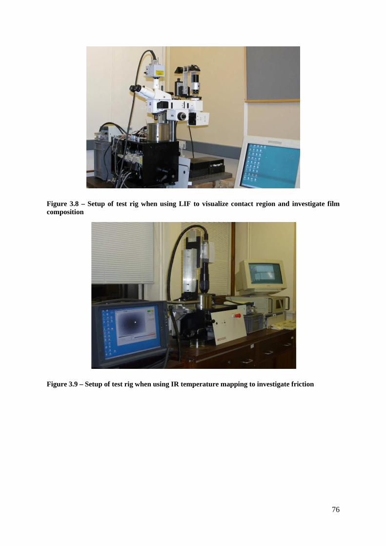
76

Figure 3.8 – Setup of test rig when using LIF to visualize contact region and investigate film composition

Figure 3.9 – Setup of test rig when using IR temperature mapping to investigate friction

77

3.2 Experimental techniques

In this section, all the experimental techniques employed in this work are described. The

three main techniques used in this study to investigate film thickness, film composition and

friction are first described. All three techniques were carried out using the modified EHL rig

described in Section 3.1.

A set of secondary techniques which aid in the analysis and characterization of the lubricants

investigated are then described. These include measurement of viscosity using various

techniques, measurement of idle ball speed as well as measurement of the oil droplet size of

the oil-in-water emulsions used.

3.2.1 Main Techniques

3.2.1.1 EHD film thickness measurement


Three methods are mainly used to measure the thickness of films formed in EHD contacts.

These are optical techniques, electrical techniques and X-ray techniques [60].

When measuring film thickness of emulsions, two techniques have been used in the past.

Optical interferometry was used when investigating point and line contacts [46-52] while an

X-ray transmission technique was used when using two or four disc machines [44, 59].

Electrical techniques such as capacitance and resistance measurements are not used when

investigating emulsions as these can be highly conducting.

3.2.1.1.2 Ultra-thin film interferometry

The technique used to measure single-phase and two-phase lubricants in this work is ultra-

thin film interferometry. This technique, which was developed in the late 1980’s at Imperial

College [61], is an improved variant of the conventional optical interferometry technique

which was first introduced in the 1960’s by Gohar and Cameron [62-64]. Ultra-thin film

interferometry is the most widely used method of measuring lubricant film thickness in EHD

lubrication as it enables the measurement of films down to 1 nm thick. [65].

78

Figure 3.10 illustrates schematically the principle of this technique. A contact is formed

between a flat rotating transparent glass disc and a steel ball. The glass disc is coated with a

semi-reflective layer of chromium and a silica layer. White light is shone into the contact

through the glass disc. Some of the light reflects off from the chromium layer while some

passes through the spacer layer and the lubricant film and is reflected from the steel ball. Due

to a path difference (which depends on the thickness of the oil film), the two reflected beams

acquire a phase difference and, when recombined, they optically interfere, causing destructive

and constructive interference.

In Figure 3.10, the angle of incidence has been exaggerated for clarity, however, in the thin

film measuring setup, the angle of incidence is zero. This, together with the fact that the

refractive index of oil and glass is very similar, ensures that the angles of incidence and

reflection are the same.

For constructive interference (angle of incidence = 0):

XnymQnym � XzT �d�QzT �d� � ®¯ � °¯, N = 1,2,3,... Equation 3.1

For destructive interference (angle of incidence = 0):

XnymQnym � XzT �d�QzT �d� � ®¯ � �° , ½�¯, N = 1,2,3,... Equation 3.2

The path difference is given by �2²(��(�� 2²7\�'�9�7\�'�9�, where ²(�� and ²7\�'�9 are the

refractive index of the oil film and spacer layer while �(�� and �7\�'�9 are the film thickness

of the oil film and the spacer layer. ³´ is the interfacial phase shift between the two beams

which occurs due to a change of refractive index of the mediums at either or both of the

Figure 3.10 - Schematic illustrating ultra-thin interferometry

glass

semi – reflective

chromium layer silica layer

h

spectrometer

reflective metal ball

79

reflecting surfaces. The oil/steel interface produces a phase shift very close to π while for the

semi-reflecting solid/oil interface, the value of the correction factor, ω, is typically between 0

and 0.2 [65].

The spacer layer, which is not utilized in conventional interferometry, ensures that

interference occurs even if no oil film is present (N > 1 even when hoil = 0) and is necessary

in order to measure fluid films that are thinner than ¼ of wavelength of the incident light.

The thickness of the spacer layer is measured prior to testing, when no oil film is present.

Each fluid film thickness is obtained by measuring the combined thickness of the spacer layer

and lubricant film, then subtracting the known spacer layer thickness. The spacer layer can

vary in thickness over the disc surface thus film thickness measurements should be taken at

the same exact position on the disc where the spacer layer thickness has been determined

(using a stationary loaded contact at the start of each test). This is achieved by triggering

measurements so that all film thickness measurements are taken from the same position on

the rotating disc circumference. The thickness of the semi-reflective chromium layer (which

is around 10 nm) is chosen so that the reflected and transmitted parts of the beam are of

approximately equal intensity on recombination.

The interfered white light is then passed into a spectrometer where its constituent

wavelengths are dispersed and detected by a camera. The spectrometer replaces the human

eye which was formerly used in conventional interferometry to identify and distinguish

colours which were then related to an approximate corresponding wavelength, thereby

allowing the wavelength of constructive interference to be precisely determined.

The light entering the spectrometer is restricted to a thin rectangular strip of the central fringe

image aligned at 90˚ to the direction of rolling by using a narrow grating (250 µm) which is

mounted on the spectrometer. The light coming from this strip is then dispersed by the

spectrometer and observed as the output from a black and white camera (see Figure 3.11).

The lighter regions correspond to constructive interference at a particular wavelength while

the darker regions correspond to destructive interference.

The wavelength-dispersed image is then captured by a frame grabber and a computer

programme averages the values within the centre of this image to produce an intensity profile

of the spectrum as a function of the wavelength. The screen position at which maximum

intensity occurs is recorded, from which, using a calibration technique, the wavelength which

80

gives maximum constructive interference at the central region of the contact can be obtained.

This wavelength is then used to calculate the mean film thickness of the central oil film.

Figure 3.11 - Setup for ultra-thin film interferometry

3.2.1.1.2.1 Calibration of spectrometer

In order to be able to convert the screen position at which maximum intensity occurs into a

wavelength which gives maximum constructive interference, the screen position indicated by

the spectrometer must be related to a calibrated wavelength.

The calibrations are carried out using a mercury lamp which provides light of a known

wavelength emission. During calibration, the whole spectrum can be scanned on the screen

by rotating the spectrometer grating using a micrometer (only a portion of the spectrum fits in

the screen as this is magnified to improve resolution).

To calibrate the spectrometer against wavelength, the micrometer was adjusted such that a

discrete waveband of the mercury lamp was placed at the same screen position (screen is

divided into a 640 value array). The micrometer reading was recorded for each waveband and

a graph of wavelength against micrometer reading was obtained (Figure 3.12 (a)), from

which calibration constants A (slope) and B (y-intercept) were derived.

When calibrating the spectrometer against screen position, a single spectral line (obtained

using the mercury lamp) was used, and the variation in screen position is noted as the

camera microscope

glass disc

steel ball load

spectrometer

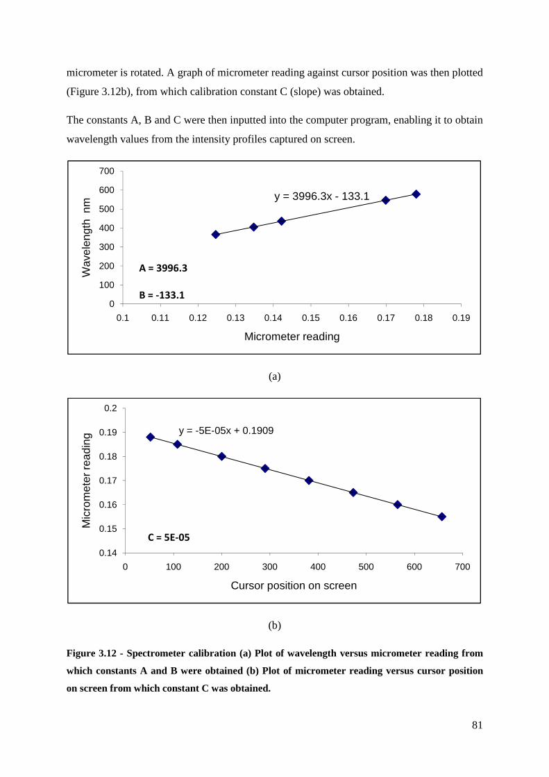
81

micrometer is rotated. A graph of micrometer reading against cursor position was then plotted

(Figure 3.12b), from which calibration constant C (slope) was obtained.

The constants A, B and C were then inputted into the computer program, enabling it to obtain

wavelength values from the intensity profiles captured on screen.

(a)

(b)

Figure 3.12 - Spectrometer calibration (a) Plot of wavelength versus micrometer reading from

which constants A and B were obtained (b) Plot of micrometer reading versus cursor position

on screen from which constant C was obtained.

y = 3996.3x - 133.1

0

100

200

300

400

500

600

700

0.1 0.11 0.12 0.13 0.14 0.15 0.16 0.17 0.18 0.19

Wav

elen

gth

nm

Micrometer reading

A = 3996.3

B = -133.1

y = -5E-05x + 0.1909

0.14

0.15

0.16

0.17

0.18

0.19

0.2

0 100 200 300 400 500 600 700

Mic

rom

eter

rea

ding

Cursor position on screen

C = 5E-05

82

3.2.1.2 Visualization of contact region and investigation of oil composition

using Light Induced Fluorescence

In this study, a fluorescence technique was used to investigate the three stages of behaviour

of oil-in-water emulsions. This was done by visually observing what phases are present at the

inlet in Stage I and II and establishing the composition of the entrained lubricant in Stages I,

II and III at the contact using intensity measurements.


Fluorescence is a phenomenon which occurs in certain molecules known as fluorophores or

fluorescent dyes. The fluorophore is excited from the ground state to a higher energy singlet

state, which then rapidly returns to the ground state by emission of a photon [66]. This

phenomenon is illustrated in Figure 3.13 and can be explained in three stages [67].

Figure 3.13 – Diagram illustrating fluorescence phenomenon [68]

Stage 1: Excitation

When a photon of energy hνEx which is supplied by an external source such as a laser is

absorbed by the fluorophore, it is excited from the ground state, S0, to a higher vibrational

energy of S1 or S2.

83

Stage 2: Excited-state lifetime

The excited state exists for a short period of time, typically 10-8s. During this time, the

fluorophore undergoes various changes, and a number of interactions with its molecular

environment occur as these excited molecules emit photons and fall back into lower energy

states.

The molecules at a high vibrational energy S2 rapidly relax to the lowest vibrational energy

level S1, which is the thermally equilibrated singlet state from which fluorescence originates.

Vibrational relaxation, or internal conversion, generally occurs in 10-12 s, and is complete

prior to fluorescence emission.

Not all the molecules initially excited by absorption return to the ground state, S0, by

fluorescent emission. Other emissions and energy transfers resulting from processes such as

intersystem crossing and quenching occur [66]. Intersystem crossing happens when the

electron undergoes a spin conversion into a triplet state instead of the lowest singlet excited

state, and emission from the triplet state occurs with lower energy relative to fluorescence.

This type of emission is also known as phosphorescence (Figure 3.13). Fluorescence

quenching refers to any process which decreases the fluorescence intensity of a given

substance. Quenching processes include excited state reactions, molecular rearrangements,

ground state complex formation and energy transfer.

The relative extent to which these processes occur is given by the fluorescence quantum

yield, which is the ratio of the number of fluorescence photons emitted to the number of

photons absorbed.

Stage 3: Fluorescence Emission

After around 10 ns, a photon of energy hνEm is emitted, returning the fluorophore to the

ground state S0. Due to energy dissipation from processes such as relaxation and excited state

reactions during the excited-state lifetime, the energy of emission is less than that of

absorption, hence fluorescence occurs at longer wavelengths. The difference in energy or

wavelength represented by (hνEx − hνEm) is known as the Stokes shift. This phenomenon is

essential to fluorescence techniques as, by using cut-off filters, one is able to distinguish

emission photons from excitation photons (Figure 3.14).

84

Figure 3.14 - Diagram illustrating Stokes shift. Due to energy dissipation during the excited

state lifetime, the wavelength of the emitted photon is higher, therefore, using a cut-off filter,

one is able to isolate the emitted energy from the excitation light (shaded region on diagram)

3.2.1.2.2 Applications of Light Induced Fluorescence

LIF is a technique which is widely used as a visualization and quantitative tool in various

fields. Fluorescent dyes are extensively used as tracers in the biochemical, medical and

chemical fields [69] to detect and observe molecules and in fluid dynamics to measure

velocity and related properties in fluids [70].

LIF has also been used in the tribology field as a visual tool to investigate particles and

lubricant flow [71] and as a quantitative tool to measure film thickness. Most of the films

measured fall in the micron range [72, 73] as, for thinner films, sensitivity issues arise [74],

making it difficult to accurately measure the thickness of films in the nanometre range, which

is the range in which EHL films fall. Very recently, measurement of film thickness in the

nanometre range was reported by Reddyhoff et al. [71] using Eosin as the fluorescent dye.

emission

cut-off filter

inte

nsi

ty

wavelength

Stokes shift

absorption

85

The total fluorescence, F, emitted by a volume of fluid, V, is given by:

µ � +�¯m zd�iZVd¶·¸ Equation 3.3

where Ie is the intensity of the light source used, λlaser is the laser wavelength, ε is the dye

absorption coefficient, Cdye is the dye concentration and φ is the quantum efficiency.

Fluorescence is therefore a function of the dye characteristics, the dye concentration, the

exciting light intensity, and the parameter being measured. Once a particular dye and

concentration are selected, the fluorescence dependence on these factors becomes constant

and the fluorescence emitted by a system can be used to characterize any other test variable

which is affected by fluorescence. A typical parameter in tribology which can be

characterized by fluorescence is film thickness of neat oil. The test lubricant is dyed and any

change in intensity during testing can be related to a change in film thickness.

3.2.1.2.3 Application of LIF for oil-in-water emulsions in high speed EHD

contacts

LIF is a very powerful visualization tool for two-phase lubricants as, by dissolving a

fluorescent dye in just one of the phases, one is able to distinguish between the two and

visually investigate the behaviour of each (Figure 3.15).

Figure 3.15 - Image of an oil-in-water emulsion obtained using LIF. The fluorophore was

dissolved in the oil phase hence bright regions denote oil droplets while dark regions denote

water.

The intensity of the fluorescent oil lubricant film can also be used as a quantitative tool to

investigate emulsion composition as, for a given volume, any change in intensity can be

related to a change in composition. Intensity measurements are particularly useful at high

speeds, since image capture is only possible at low speeds due to the limitations of cameras

86

(frame rates of sufficiently sensitive CCD cameras rarely exceed 2000 frames per second).

Thus, characterization by LIF of oil-in-water emulsions at high speeds is restricted to

measurements of the average intensity and mainly relies on the use of LIF to obtain intensity

measurements.

When using LIF to obtain intensity measurements, various experimental factors have to be

taken into account. First of all, not all the intensity emitted is captured by the camera, as is

assumed in Equation 3.3 hence, this equation cannot be directly used to obtain information

about the parameter being investigated. Another issue is that the intensity of the exciting light

can vary with time. The latter effect is commonly experienced when using lasers. The

conditions at the contact could also cause effects such as reflection from the ball metal

surface, reabsorption and scattering, all of which affect the measured intensity. Variations in

intensity could also arise from a slight misalignment or change in focus of the system being

used. Moreover, the intensity values obtained are dependent on the properties of the camera

used to capture the emission. Therefore, if some settings such as gain, aperture speed, size of

images etc, need to be modified during testing, the intensity measurements will be

compromised. Thus, although one aims to keep every factor constant throughout testing, this

may be quite difficult to achieve. In order to use intensity values and correlate them to actual

composition, strict calibration, ratiometric and normalizing techniques are essential [73]. One

simple approach to avoid these issues is to use the trend of the intensity measurement

obtained during testing rather than the absolute measured values to investigate the behaviour

of the emulsion. Once the test has started, the environment does not change so any variation

in intensity obtained during testing can be correlated to changes happening at the contact.

87

Figure 3.16 shows a schematic diagram of the experimental setup used in this study to

investigate the behaviour of oil-in-water emulsions.

Figure 3.16 - Schematic diagram of the experimental setup used when using LIF

The exciting light (coming from a class 3B 532 nm continuous laser) is focused on the

contact using a series of lenses. When the laser light reaches the fluorophores dissolved in the

lubricant at the contact, fluorescent light is emitted. This is captured by a high-speed camera

(which can reach 2000 fps), from which images and intensity values of the area being

observed can be obtained. No exciting light, which has a lower wavelength, reaches the

camera as this is filtered out by using a dichroic which cuts off any wavelengths lower than

the wavelength at which maximum emission occurs (see Figure 3.14).

All the lenses and filters were mounted on a single stage so as to keep misalignment to a

minimum. Once the laser was aligned and focused, all the tests were run without changing

any of the settings. (Note: One change that could happen in between tests is due to the

refocusing on the contact whenever test specimens are changed. The objective lens must be

raised up to allow for test specimens and test lubricant to be replaced.)

Excitation

Fluorescence

high speed camera

dichroic

mirror

excitation filter

stops

lenses

collimator

objective

532 nm continuous laser

88

3.2.1.2.3.1 LIF as a visualization tool

When using LIF as a visualization tool, tests were run for a range of speeds (0.02 - 0.8 m s-1)

using the dyed test lubricant and videos of the contact region (which included the whole area

from outside the inlet to the outlet) were taken. Videos were used to investigate the behaviour

of the oil droplets in the emulsion and their direction of flow as they approached the contact

region (Figure 3.17).

Figure 3.17 - Typical image obtained when using LIF to visualize the inlet region. The dye was

dissolved in the oil, enabling the visualization of the oil being entrained in the contact and the

water (dark area) being squeezed away from the contact.

When performing visual observations, particular attention was paid to the inlet region, as this

is the region from which lubricant is entrained in the contact. When observing the inlet

region, the camera was kept on a fixed area to enable an assessment of the variation of the

pool inlet distance without the risk of varying the area being examined.

All of the imaging was performed using an oil-soluble dye. This was preferred to a water-

soluble dye since it allowed the oil droplets to be identified without being obscured by

emission from the continuous aqueous phase. The area of contact appears dark in the image

because the thickness of the lubricant film here is very low, so little light is emitted

irrespective of the composition.

The speed up to which visual observations could be carried out was limited by the frame rate

of the camera being used (2000 fps), making imaging of the contact region achievable for

speeds of up to around 0.8 m s-1.

89

3.2.1.2.3.2 LIF intensity measurements

To investigate the behaviour of emulsions at high speeds, where Stage III behaviour is

predominant, the mean intensity of emission from the area of contact was measured. This was

used to provide an indication of the variation in composition with speed.

The contact area was located at low speeds and, once the camera was focused on the contact

region, it was not moved as the speed was increased. A series of images were then taken for

each speed, from which the average intensity at the contact was obtained. Tests were run up

to speeds of 20 m s-1 using neat oil, a dilute 3% oil-in-water emulsion and a 40% oil-in-water

emulsion. The neat oil test was done so as to have a reference intensity value for neat oil

whereas a static image of the contact fully immersed in dyed water was used to obtain a

benchmark intensity value for pure water. All the tests were done consecutively, without

changing any camera or laser settings so as to try and reduce discrepancies in intensity

measurements due to change in the alignment of setup etc. as much as possible. The set of

tests were carried out twice; once using an oil-soluble dye and a second time using a water-

soluble dye. This was done to enable a better interpretation of how the oil content and water

content vary in the contact as the speed is increased.

(a) (b)

Figure 3.18 - Images obtained using the same test conditions (speed = 0.03 m s-1) using (a) an oil-

soluble dye and (b) a water-soluble dye.

90

3.2.1.3 Friction measurement

The most widely used way of measuring friction in EHD contacts at low speeds is to measure

the tractive force at the contact using displacement/force or torque transducers, from which

the traction coefficient is obtained. Initially, strain gauges were fitted to the rig to measure the

tractive force at high speeds. With this technique, however, some difficulties were

encountered in transmitting the signal at high rotational speeds hence a convenient alternative

approach to mechanical traction measurement was used in this study.

An infrared temperature mapping technique was used to measure the surface temperature,

from which friction can then be determined. This is possible since almost all of the energy

dissipation (and hence temperature rise) within a rolling-sliding contact results directly from

the shear (and thus the friction) of the fluid film, therefore, if the surface temperature is

known, local shear stresses and friction values can be determined. In addition to determining

the average friction, this technique also provides the temperature conditions in the contact

region which are also of considerable importance to the traction behaviour of the lubricant.

None of the other direct friction measurement techniques provide such information of the

contact.

Infrared temperature mapping was first used in the 1970’s by Sanborn and Winer [75-77] and

was further developed in the 1990’s [78-81] by Spikes and co-workers to enable the

determination of EHD traction with an accuracy that is comparable to that obtained with

direct traction measurement techniques [82].

In this section, the infrared temperature mapping technique is described, detailing all the

issues which had to be addressed when applying this technique to investigate neat oil and oil-

in-water emulsions at high speeds.

91

3.2.1.3.1 Infrared Temperature mapping

3.2.1.3.1.1 Introduction

The procedure carried out to obtain temperature maps and friction consists of three main

steps. The first step is to measure infrared emission while a test is being run. The

measurements are then converted into temperature rise and finally the temperature rise is

used to calculate local shear stresses and friction. These steps are described in some detail in

the following sections.

3.2.1.3.1.1.1 Measuring IR emission

An infrared (IR) camera is used to measure and map thermal emission from the steel and

sapphire surfaces in a sliding EHD contact between a steel ball and a sapphire disc.

The camera used for this work is sensitive to IR of wavelength from 3 to 5µm (and is

therefore sensitive to emission from both oil and steel components) and, with the setup used

during testing (320 × 256 focal plane array combined with the ×5 objective lens), provides a

resolution of 6.3µm/pixel. The Hertz contact diameter during all testing was around 256µm

(point contact, 20N); hence 32 × 32 temperature readings were taken within the contact.

In recent studies carried out [82, 83], the sapphire disc used during testing consisted of three

segments, each having a different coating (see Figure 3.19). One sector was uncoated, the

second sector was coated with a thick layer (120 nm) of chromium and the remaining sector

was coated with a layer of aluminium.

Three IR emission readings were thus obtained for each test carried out. With the uncoated

sector of the sapphire disc, most of the IR emission detected by the camera originates from

Al coating

Uncoated

Cr coating

Figure 3.19 - Sapphire disc used during testing

sapphire disc

92

the steel ball and can thus be used to determine the temperature of the steel ball surface.

When the chromium-coated sector is in the contact, the emission measured originates from

the sapphire disc surface and thus gives a measure of the temperature of the disc surface.

Although most of the detected radiation originates from the steel ball or chromium-coated

sapphire surfaces, some is emitted from the bulk of the sapphire disc. Aluminium has a very

low emissivity, thus, the aluminium-coated sector will only allow radiation from the bulk

sapphire disc to reach the camera and is therefore used to determine the radiation emitted

from the bulk of the sapphire disc itself.

The IR emission from the bulk of the sapphire disc is taken as the IR measurement obtained

with the aluminium coating minus one tenth of that measured with the chromium coated

sector so as to take into account the low emissivity of aluminium. This is then deducted from

the measured IR emission from the chromium and steel surfaces for temperature calculation

so that the bulk temperature effect is eliminated and more accurate values for the

temperatures of the ball and disc surfaces can be obtained.

In addition to the three emissions described in this section, a small amount of radiation

coming from the lubricant film is also detected by the IR camera. This was removed by using

a transmission filter which cuts off any radiation of wavelength below 3.75µm. The choice of

filter was based on previous work which showed that the narrow bandwidth of wavelength at

which IR is emitted by the lubricant is below 3.75µm [77, 81, 84].

93

3.2.1.3.1.1.2 Conversion of IR emission to temperature maps

The emission measurements are converted to temperatures using a calibration technique.

A set of tests are run (using neat oil) in pure rolling at a series of controlled lubricant

temperatures (20-85˚C). Since, in pure rolling, frictional heating is negligible, the in-contact

surface temperature is the same as the controlled oil temperature. Surface temperature can

therefore be directly related to surface radiation for both the steel ball and the chromium

coating. A graph of IR emission (camera counts) detected by the IR camera (corrected using

aluminium coating) against temperature is obtained for the uncoated (measuring steel ball

surface temperature) and the chromium coated segment of the sapphire disc, from which two

calibration equations are obtained (Figure 3.20).

Figure 3.20 - Plot of temperature against IR emission (camera counts) detected by the IR

camera (corrected using aluminium coating) obtained for the uncoated (measuring steel ball

surface temperature) and the chromium coated segment of the sapphire disc. The two

calibration equations used to convert the IR emission from the two disc segments to

temperature are displayed on the graph.

The calibration equations are used throughout all testing to convert all measured IR emissions

into ball and disc surface temperatures.

T Uncoated = 41.387ln(Un-Al) - 262.39

T Chromium = 51.25ln(Cr-Al) - 315.9

0

10

20

30

40

50

60

70

80

90

0 1000 2000 3000 4000 5000

Tem

pera

ture

of o

il at

inle

t ºC

No of counts from camera (Al coating subtracted)

Uncoated disc

Chromium coated disc

94

3.2.1.3.1.1.3 Determination of shear stress maps and friction from surface

temperature maps using moving heat source theory

The shear stress calculation technique was first described in detail in [78, 79] for 1D analysis

and in [80] for 2D analysis and is based on the principle that, in fluid shear, the local rate of

heat generation in a columnar volume of fluid of unit area within the contact, @A , is given by:

¹A � �∆Y Equation 3.4

where τ is the mean shear stress through the film and ∆1 is the sliding speed.

This technique assumes that this heat passes rapidly into the two bounding surfaces (Figure

3.21) by conduction such that:

¹A �nZ zºddm � mm � ¹A �nZ z TTQy�d Zyz� � �∆Y Equation 3.5

where @A'()� 7»�� ¼�� and @A'()� 7�\\$�9� ��7' are the rates of heat input into the steel ball and

sapphire disc surfaces respectively.

This assumption is valid if the ratio of heat conducted to heat convected from the lubricant is

high and is further discussed in Section 3.2.1.3.1.4.1. If the rates of heat input are known, the

shear stress can then be calculated.

The calculation of @A steel ball and @A sapphire disc is based on the work of Jaeger [85], which gives

equations for the temperature rise of the surface of a body due to a moving uniform heat

input.

disc surface @A��7'

ball surface

@A¼��

Figure 3.21 - Heat generated in a fluid element

95

The contact is treated as an array of many separate, rectangular heat sources, collectively

forming the overall heat input to the moving surfaces. This is done to take into account the

fact that heat input into the solid surfaces varies across the contact (Jaeger’s equations apply

for a uniform heat source). In this analysis, each element consists of two temperature rise

measurements. This was necessary as otherwise, if each measurement on the temperature

map is taken to be at the centre of a separate heat source, the processing time would have

been excessively long.

Jaeger provides a means of calculating the influence of heat input to the moving surface at

one location qkl on the temperature rise at any other point on the surface, Tij:

½hy¾ � iy¾�m¹A �m Equation 3.6

where �� is the influence coefficient of heat input into an area on the surface on temperature

at any other point on the surface and is given by:

iy¾�m � WX¿�z À dOTª� YzXÁzÂ�OÃy�O��5Ã�Ä«

� ZO�′ ZVm′ Equation 3.7

where A is the area of the element, (xi , yj) is the location of the temperature rise, (xk, yl) is the

location of the heat input, R is the distance between the point of heat input and the point of

temperature rise and is given by: ((xk − xi)2 + (yl − yj)

2)1/2. Us is the speed of the surface

relative to the heat source, ks is the thermal conductivity of the surface material, and χs is the

thermal diffusivity of the surface material which is given by 27 E7F7⁄ . The thermal properties

of both the steel ball and sapphire disc are given in Table 3.1.

Thermal properties Steel ball Sapphire disc

Ås J/kg K 420 753

ks W/mK 30 24

Æs kg/m3 7860 3985

Table 3.1- Thermal properties of steel ball and sapphire disc

96

The overall (measured) temperature rise at one point is given by the sum of the influence of

all the heat inputs within the contact:

∆hy¾ � ∑ iy¾�m¹A �m�m Equation 3.8

Thus, once a matrix of calculated influence coefficients is obtained, Equation 3.8 can be used

to convert temperature maps, which give the overall temperature rise at each point on the

contact, into maps of heat input.

Before applying Jaeger’s equations, the temperature rise maps were smoothed three

successive times using a weighing approach to each element (i,j).

hy¾ � ��hy¾ 5hyÈW,¾5hyÉW,¾5hy,¾ÈW5hy,¾ÉW�b Equation 3.9

where the four terms refer to neighbouring elements.

This was done to filter any local fluctuations in the measured temperature caused by the

slight variation between sensors within the camera’s focal plane array.

Once the rate of heat input for each point within the contact is known, shear stress maps are

easily determined using Equation 3.5. Shear stress maps can then be used to obtain the

overall friction. This is determined by integrating the shear stress, τ, developed in the

lubricant film over the contact area and then dividing by the applied load.

The code utilized to convert the IR emissions into shear stress maps and friction was already

available [82] and was only slightly modified to take into account convection losses where

necessary (see Section 3.2.1.3.1.4.1).

3.2.1.3.1.2 Main assumptions in IR surface mapping technique

This technique makes two main assumptions:

1. all heat generated passes rapidly by conduction into the bounding surfaces; and

2. all heat is generated by fluid shear (none by compression)

The first assumption was mentioned earlier and is discussed in section 3.2.1.3.1.4.1. As

regards the second assumption, the contribution to heating and friction of fluid compression

97

is generally negligible for sliding contacts. The heat generated by compression in a column of

fluid is given by [83, 86]:

¹A � ÊhQnymY ZTZO Equation 3.10

where ε is the coefficient of thermal expansivity of the oil, T the absolute temperature

(degrees Kelvin), hoil the oil film thickness, U the mean rolling speed, and dp/dx is the

pressure gradient in the rolling/sliding direction.

If one examines the energy equation [7], it can be shown that the magnitude of the

compression term is much smaller than the shear term. This has also been demonstrated

experimentally using infrared measurements taken under nearly identical conditions as the

ones used in this study [87]. The above reasons justify why compressive heating was not

taken into account in this thesis.

3.2.1.3.1.3 Validation of technique

Since infrared temperature mapping determines friction in an indirect way, it was felt

important to validate this method. This was done by comparing the calculated friction

obtained using the infrared temperature mapping technique to friction measurements obtained

using a more established method which measures friction directly by using strain gauge

systems and a torque transducer .

Figure 3.22 shows the traction values obtained using the infrared temperature technique

compared to direct friction measurements. Both tests were carried out on the EHL rig (using

ball and disc setup) under the same test conditions. Direct friction measurements were

obtained by using a strain gauge system to measure the frictional torque on the ball shaft of

the EHL rig. The traction software logs data from the ball torque and load transducers and

calculates the resulting traction coefficient. Friction values obtained with the infrared

mapping technique are only shown for speeds of 0.21 m s-1 and above as, below this speed,

the calculated friction values are noisy due to the low temperature rises involved. The strain

gauge system used in the direct friction measurement method was limited to speeds of up to

1.5 m s -1, hence, comparison of the results obtained using both methods is available for

speeds between 0.21 m s -1 and 1.5 m s -1.

98

Figure 3.22 - Plot showing traction coefficient for neat oil obtained using the infrared

temperature technique compared to direct friction measurements obtained on the EHL rig

using a strain measurement technique

(Test parameters: contact: point, load: 20N, temperature: 40˚C, slide-roll ratio: 0.5, oil: mineral, group I)

The calculated friction results obtained using the infrared measurement technique are very

similar to those obtained with the direct friction measurement technique, showing that the

technique used in this work gives friction values which are comparable to those obtained with

established direct friction measurement methods.

0

0.05

0.1

0.01 0.1 1 10

Trac

tion

coef

ficie

nt


strain gauge measurement technique

IR surface temperature mapping technique

99

3.2.1.3.1.4 Adaptation of IR technique to measure neat oil and oil-in-water

emulsions at high speeds

In order to be able to use the IR temperature mapping technique for this study, a number of

issues related to the severe test parameters (high sliding and entrainment speeds) and the

composition of the lubricant tested (oil and water content) had to be addressed. These issues

are described and discussed in the following section.

3.2.1.3.1.4.1 High sliding and entrainment speeds

Due to the high speeds being investigated, the use of a disc with three differently coated

segments was not possible since the exposure time of the IR camera was not high enough to

record emission from all three sections successively as the disc rotated. Three separate

sapphire discs were used instead, one uncoated, one chromium coated and one aluminium

coated. Each test was repeated three times so that IR emissions from the disc surface, ball

surface and bulk sapphire disc were obtained for each test condition investigated.

As the aluminium coating peels off very easily, this becomes severely damaged with the test

parameters used (high speeds and sliding), making it impossible to obtain IR measurements

in the contact area. The emission readings from the aluminium coated sapphire disc are

therefore taken at one half Hertz diameter to the side of the contact. In this region, the coating

remains intact, allowing IR measurements to be taken for the whole range of speeds

investigated.

As mentioned in Section 3.2.1.3.1.1.3, the IR temperature mapping technique assumes that all

the heat generated passes rapidly by conduction into the bounding surfaces. For this

assumption to hold, the main mode of heat transfer within the contact must be conduction.

Cameron [88] showed that the ratio of heat conducted to heat convected from a thin film of

lubricant is given approximately by:

��nZ��n^ � �m�� g

Æm��Åm��YQX Equation 3.11

where klub, Elub and Flub are the thermal conductivity, density and specific heat capacity of the

lubricant respectively, U is the entrainment speed, h is the film thickness and B is the length

of film in the convection direction. When calculating shear stresses, B is taken as 12.6 µm,

which is the size of each fluid element in the contact area.

100

Table 3.2 shows the corresponding values for oil and water for the thermal properties used in

Equation 3.11.

When running tests using oil-in-water emulsions, the conduction to convection ratio is greater

than 50 for all the range of speeds investigated, hence Equation 3.5 can be used to calculate

local shear stresses. However, when running tests at high speeds using neat oil, thick films

(which can reach up to 1µm) are formed within the contact. As can be seen from Equation

3.11, the higher the film thickness, h, the lower the conduction to convection ratio. Table 3.3

shows the conduction to convection ratio for a mineral oil as the entrainment speed is

increased.

h nm U m s-1 Hcond/Hconv

364 2.2 22.0

428 3.1 11.4

515 4.3 5.67

597 6.0 3.04

677 8.4 1.70

757 11.8 0.98

824 16.5 0.59

Table 3.3 - Table showing film thickness and calculated conduction to convection ratio for

mineral oil at each corresponding entrainment speed (B = 12.6 µm)

Thermal Properties oil water

Ålub J/kg K 1867 4187

klub W/m K 0.104 0.58

Ælub kg/m3 900 1000

Table 3.2 - Thermal properties of oil and water

101

The conduction to convection ratio is very low at speeds above 4 m s -1. This means that a

considerable amount of heat generated in the fluid element is convected to the surrounding

area in the direction of rolling/sliding rather than being mostly conducted to the surfaces. The

measured IR emission is therefore just a fraction of the heat developed in the contact. To take

this condition into account, two terms, @A'()* ��,� and @A'()* �5�,� are added to Equation 3.5

such that:

¹A ºnº m y¾ � ¹A �nZ Zyz� y¾ � ¹A �nZ � mm y¾ , ¹A �n^ y�W,¾ � ¹A �n^ y5W,¾ Equation 3.12

These additional terms represent the heat entering and exiting the fluid element by convection

in the rolling/sliding direction (Figure 3.23).

The convection terms are taken as a function of the conduction terms which are obtained

using the measured emissions of the ball and disc and, using Equation 3.11, can be defined

as:

¹A �n^ � ¹A �nZ Ænym Ånym� g �nym Equation 3.13

@A'()� ¼��

@A '()� ��7'

@A'()* �5�,�

disc surface

ball surface

@A'()* ��,�

Figure 3.23 - Heat generated by fluid element taking into account heat transfer by

convection to and from neighbouring elements in the rolling/sliding direction

102

Hence the two convection terms in Equation 3.12 can be defined as:

¹A �n^ y�W,¾ � ¹A �nZ � mm yÉW,¾ Ænym Ånym� g �nym � ¹A �nZ Zyz� yÉW,¾ Ænym Ånym

� g �nym Equation 3.14

¹A �n^ y5W,¾ � ¹A �nZ � mm yÈW.¾ Ænym Ånym� g �nym � ¹A �nZ Zyz� yÈW,¾ Ænym Ånym

� g �nym Equation 3.15

Thus, when converting temperature maps obtained using neat oil, Equation 3.12 rather than

Equation 3.5 is used to calculate local shear stresses.

It was found that convection losses affect the shape of the calculated shear stress distribution,

however, the integral of the shear stress is largely unaffected (see Section 5.1.3.2). Since the

overall friction is found from the integral of the shear stress, it is independent of whether

convection has been taken into account. Another way of looking at this is that, when

obtaining the overall friction, the contact is treated as a whole. The ratio of convection to

conduction is then calculated using a value of B that is equal to the diameter of the contact

(256 µm) rather than using the size of the fluid elements (12.6 µm), as is done for shear stress

calculations. This gives a ratio of conduction to convection that is greater than 10 throughout

the whole range of speed investigated.

3.2.1.3.1.4.2 Possible water content in entrained lubricant

When running tests with oil-in-water emulsions, it is possible that water is entrained into the

contact. This is highly likely at high speeds, where it is believed that the entrained film

consists mainly of water (Section 5.2). Water, however, does not transmit infrared radiation

therefore, if it is present at the contact, any radiation coming from surfaces below the

lubricant film may not be captured by the IR camera.

As a result of this, the IR emission from the ball surface cannot be measured by the IR

camera which is positioned above the disc. When investigating oil-in-water emulsions it will

therefore be assumed that the temperature of the ball is equal to that of the measured disc

surface. This is a reasonable assumption to make for thin films and has been made in

previous work [81], where only the temperature of the ball was measured. Both disc and ball

surface temperatures will therefore be determined from the IR emissions obtained using the

chromium and aluminium coated discs.

103

In previous works where both the ball and disc surface temperatures were measured, it was

shown that the surface temperatures differed slightly from each other, with the faster surface

usually being hotter than the slower surface [82]. This implies that, if only the disc surface

temperature is measured when calculating the coefficient of friction of oil-in-water

emulsions, the level of accuracy will be reduced. It was therefore felt important to see to what

degree the use of two IR measurements (IR emissions using aluminium and chromium coated

discs) rather than three measurements (IR emissions using aluminium coated, chromium

coated and uncoated discs) would affect the calculated overall friction coefficient.

Figure 3.24 shows the calculated friction for neat (mineral) oil obtained using measured IR

emissions of the disc surface compared to the friction values calculated using the IR

emissions of both the ball and the disc surface.

Figure 3.24 - Plot showing calculated traction coefficient calculated for neat oil obtained using

measured IR emissions of the disc surface compared to the traction coefficient calculated using

the IR emissions of both the ball and the disc surface.

(Test parameters: contact: point, load: 20N, temperature: 40˚C, slide-roll ratio: 0.5, oil: ester A)

The calculated friction values obtained using two surfaces (chromium, aluminium) are very

close to those obtained using three surfaces (chromium, aluminium, steel), suggesting that the

ball and disc surfaces are at a similar temperature. This shows that, even when measuring just

the disc surface friction, the accuracy of the calculated friction is still considerably high and

valid friction values are obtained.

0

0.005

0.01

0.015

0.02

0.025

0.03

0.035

0.1 1 10 100

Trac

tion

coef

ficie

nt


Using disc and ball temperatures

Using disc temperature only

104

3.2.2 Secondary techniques

3.2.2.1 Viscosity measurement

Viscosity can be measured using a number of techniques which are based on different

principles. Two of the most typical types are capillary viscometers and rotational

viscometers.

In this study, three commercial rotational viscometers were used. The Stabinger viscometer

(Anton Paar, [89]) was used to measure the viscosity of neat oil at various temperatures, a

rheometer with a cone and plate configuration (TA Instruments, [90]) was used to measure

the viscosity of oil-in-water emulsions while an ultra high shear viscometer (PCS

Instruments, [91]) was used to measure the viscosity of neat oils at high shear to investigate

whether they shear thin at high shear rates.

The principle of viscosity measurements of all three viscometers used in this work is based

on the measurement of the torque produced by the lubricant. Two surfaces (two coaxial

cylinders in the case of the Stabinger viscometer and the ultra shear viscometer, a cone and

plate for the cone-on-plate viscometer) are separated by the fluid under test. The two surfaces

rotate at a different speed such that the fluid creates viscous drag on the slower moving

surface. A brake torque system is present in all three viscometers. This balances the torque

applied by the moving fluid. The torque is measured by the system and is used together with

the geometry of the two surfaces to obtain the viscosity of the liquid under test.

A schematic of each viscometer is shown in Figures 3.25 (a), (b) and (c). The Stabinger

viscometer is commonly used to measure viscosity of oils as it enables quick measurement of

viscosity at a wide range of temperatures and its setup allows the measurement of the density,

hence, the kinematic viscosity together with the viscosity index can also be obtained. The

maximum shear rate reached by this viscometer is in the 106 s-1 range. The cone-on-plane

viscometer gives constant shear rate in the whole sample and was chosen when testing

emulsions as its setup allows the visual inspection of the lubricant between the cone and

plate, therefore, the test emulsion could be observed before and after testing to ensure it was

not separating during testing. The ultra shear viscometer is equipped with a high speed motor

which can reach up to 20,000 rpm and an electromagnetic clutch which engages the rotor for

only a very short period of time (typically 30 ms). The very brief shearing interval minimizes

the shear heating in the lubricant, enabling viscosity measurements to be obtained at very

105

high shear rates (up to 107 s-1). Full details of the three commercial viscometers can be found

in [89] [90] [91].

(a)

(b)

(c)

Figure 3.25 - Schematic of (a) Stabinger (from [89]) (b) cone-on-plane configuration (c) ultra

shear viscometer (from [91])

outer tube

(rotated at constant speed)

copper housing

test fluid magnet

freely floating rotor (measured speed)

rotation

drive shaft

torque spring

cone angle

(exaggerated)

cone

plate

test fluid

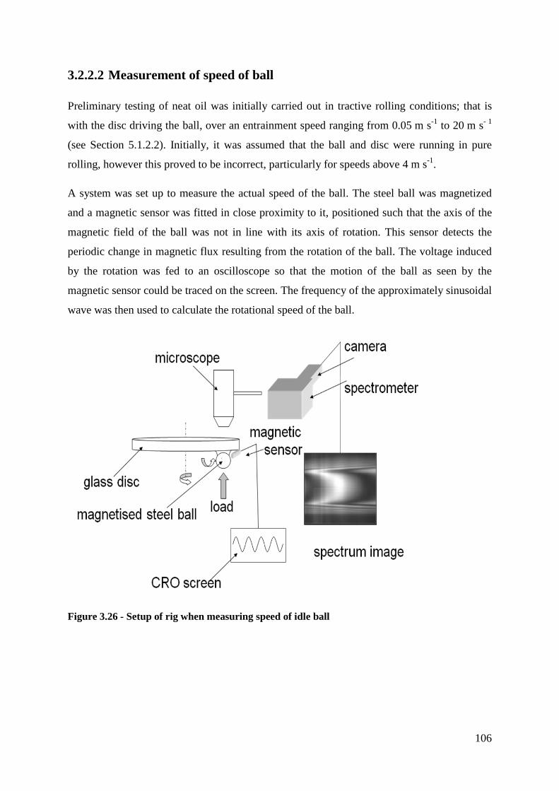
106

3.2.2.2 Measurement of speed of ball

Preliminary testing of neat oil was initially carried out in tractive rolling conditions; that is

with the disc driving the ball, over an entrainment speed ranging from 0.05 m s-1 to 20 m s- 1

(see Section 5.1.2.2). Initially, it was assumed that the ball and disc were running in pure

rolling, however this proved to be incorrect, particularly for speeds above 4 m s-1.

A system was set up to measure the actual speed of the ball. The steel ball was magnetized

and a magnetic sensor was fitted in close proximity to it, positioned such that the axis of the

magnetic field of the ball was not in line with its axis of rotation. This sensor detects the

periodic change in magnetic flux resulting from the rotation of the ball. The voltage induced

by the rotation was fed to an oscilloscope so that the motion of the ball as seen by the

magnetic sensor could be traced on the screen. The frequency of the approximately sinusoidal

wave was then used to calculate the rotational speed of the ball.

Figure 3.26 - Setup of rig when measuring speed of idle ball

107

3.2.2.3 Measurement of emulsion droplet size

The size and size distribution of the oil droplets in an emulsion are important characteristics.

Droplet size is used to assess the stability of the emulsion and is a required parameter in one

of the theories suggested for Stage III behaviour (dynamic concentration theory, [53]).

In this study, droplet size and size distribution were measured using a laser diffraction

technique. This method is based on the fact that, when particles pass through a laser beam,

these scatter light at an angle that is inversely proportional to their size. Small particles

diffract light through wide angles while larger particles scatter light at narrow angles. The

equipment used in this study was a Malvern Mastersizer 2000 Particle Size Analyzer with a

data handling package. Figure 3.27 shows a schematic of the optical system used in the

Malvern instrument [92].

Figure 3.27 - Schematic of optical system of Malvern instrument (from [92])

Particles which are located in a sample dispersion unit are passed through a focused laser

beam. This illuminates the particles which in turn scatter light at an angle that is dependent

on their size. The angular intensity of the diffracted light is then measured using a number of

photosensitive silicon detectors which are positioned in a logarithmic sequence and cover an

angular range of 0.02 degrees - 135 degrees. The map of scattering intensity against angle is

then processed by the data handling software which, using a scattering model to predict the

scattering of particles, calculates the particle size distribution. This technique allows accurate

measurement of particle size over a wide size range, namely between 0.02 -2000 µm with an

accuracy of ± 1%.

focal plane

detector

back scatter detectors

red light

source

large angle

detectors blue light

source

108

3.3 Test conditions and lubricant characteristics

3.3.1 Test conditions

In this section, all the conditions used during testing are described. A number of test

parameters have been investigated in this study hence test conditions vary during testing. In

this chapter, the range covered for each test parameter is given. The specific test conditions

used for each test carried out are then given with each plot presented in the Results chapter

(Chapter 4).

3.3.1.1 Contact geometry

Although metal rolling is best represented by a line contact, one must keep in mind the

limitation of the test rig. To be able to use line contacts on an EHL rig, the width (in the

rolling direction) of the contact cannot be low compared to the pixel size, otherwise

visualization (and therefore measurement) of the region of contact would not be possible.

However, if the width is increased so as to allow film thickness, friction and intensity

measurements, higher loads are required. In turn, these might either exceed the capability of

the loading system or lead to excessive bending in the disc/shaft assembly. In contrast, a

circular point contact is the most convenient type of contact to use on the EHL rig since

lower loads need to be applied to produce the pressures required and no alignment problems

will be encountered. Elliptical contacts, which can be obtained by using a crowned roller, are

a compromise between line and circular contacts. Whereas an elliptical contact represents a

line contact better, lower loads, which are within the equipment’s limits, would be required.

Moreover, an elliptical contact avoids the difficulties associated with the ends of line contacts

where conditions are difficult to predict and are dependent on the degree of alignment

between the disc and roller. It was therefore decided that a circular point contact and an

elliptical contact would be used in this study.

A 19 mm diameter steel ball of RMS surface roughness 11 nm was loaded against the disc to

create a circular contact while a tapered roller having an ellipticity ratio of 3.6 and RMS

surface roughness of 19 nm was loaded against the disc to create an elliptical contact. A new

steel ball or roller was used for each test carried out.

109

3.3.1.2 Temperature

Three test temperatures were used when investigating neat oil: room temperature (14˚ C),

40˚C and 100˚C. When investigating oil-in-water emulsions, the test temperature was

maintained at 40˚C throughout all tests carried out.

3.3.1.3 Load

A load of 20N was applied to each test carried out in this study. This corresponds to a

maximum contact pressure of 0.52 GPa when using the circular contact and 0.22 GPa when

using the elliptical contact.

3.3.1.4 Slide-roll ratio

A range of slide-roll ratios was investigated in this study. When measuring friction, slide-roll

ratio ranged from 0.3 to 0.8 when investigating neat oil and was kept constant at 0.8 when

investigating oil-in-water emulsions. This ensured that the temperature rise in the contact due

to shearing of the lubricant was high enough to be detected by the IR camera. All LIF work

was carried out in pure rolling conditions whereas, when measuring film thickness, slide-roll

ratio ranged from 0 to 1.9 when testing neat oils and from 0 to 1.2 when investigating oil-in-

water emulsions.

3.3.1.5 Lubricant Composition

Five oils were investigated in this study (see Section 3.3.2). The synthetic poly-alfa-olefin

(PAO) oil, group I and group III mineral oils were only tested in neat form. The two

emulsifiable ester oils were tested in both neat and emulsion form. Various oil concentrations

were used when testing the emulsifiable ester oil in emulsion form, namely: 0.5% oil, 3% oil,

20% oil and 40% oil. Most of the investigations with emulsions were carried out using 3% oil

and 40% oil as this provided a clearer contrast of any differences in behaviour.

3.3.1.6 Entrainment speed

The EHL rig used in this study enabled the ball (or roller) and disc to be run at entrainment

speeds in the range of 0.05 m s-1 to 20 m s-1. However, due to the various limitations

associated with the three main techniques used in this study, different ranges of speed were

covered during testing.

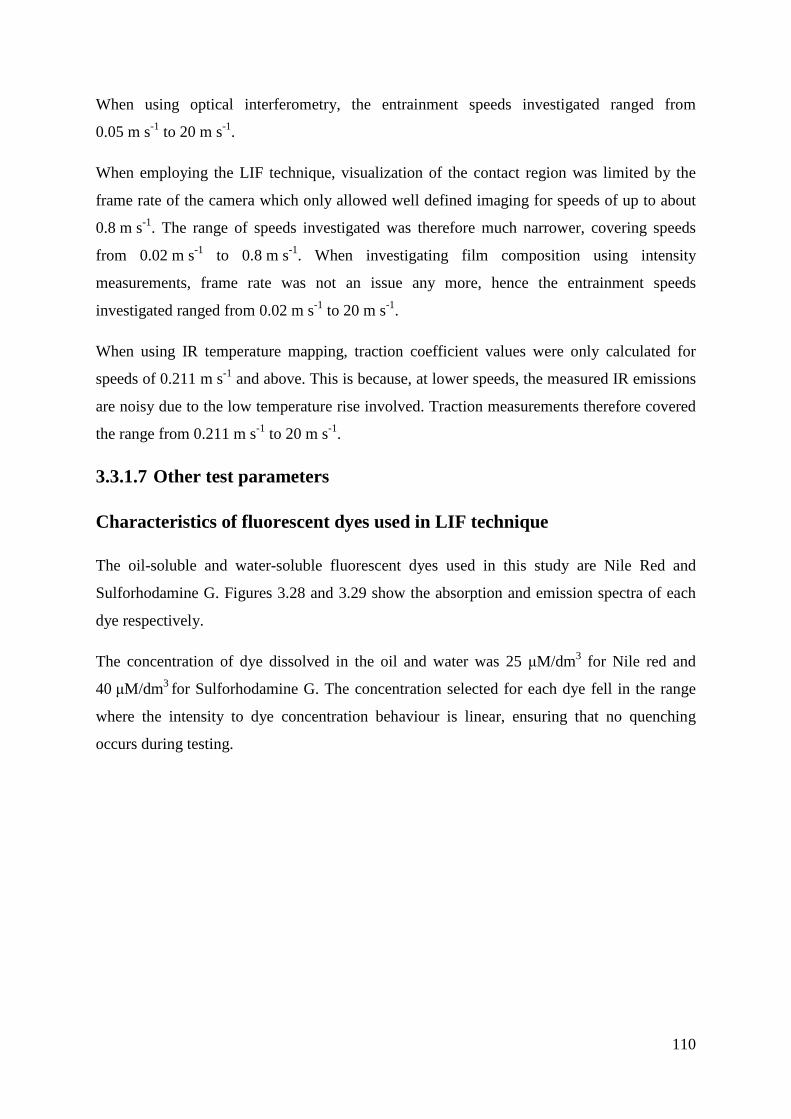
110

When using optical interferometry, the entrainment speeds investigated ranged from

0.05 m s-1 to 20 m s-1.

When employing the LIF technique, visualization of the contact region was limited by the

frame rate of the camera which only allowed well defined imaging for speeds of up to about

0.8 m s-1. The range of speeds investigated was therefore much narrower, covering speeds

from 0.02 m s-1 to 0.8 m s-1. When investigating film composition using intensity

measurements, frame rate was not an issue any more, hence the entrainment speeds

investigated ranged from 0.02 m s-1 to 20 m s-1.

When using IR temperature mapping, traction coefficient values were only calculated for

speeds of 0.211 m s-1 and above. This is because, at lower speeds, the measured IR emissions

are noisy due to the low temperature rise involved. Traction measurements therefore covered

the range from 0.211 m s-1 to 20 m s-1.

3.3.1.7 Other test parameters

Characteristics of fluorescent dyes used in LIF technique

The oil-soluble and water-soluble fluorescent dyes used in this study are Nile Red and

Sulforhodamine G. Figures 3.28 and 3.29 show the absorption and emission spectra of each

dye respectively.

The concentration of dye dissolved in the oil and water was 25 µM/dm3 for Nile red and

40 µM/dm3 for Sulforhodamine G. The concentration selected for each dye fell in the range

where the intensity to dye concentration behaviour is linear, ensuring that no quenching

occurs during testing.

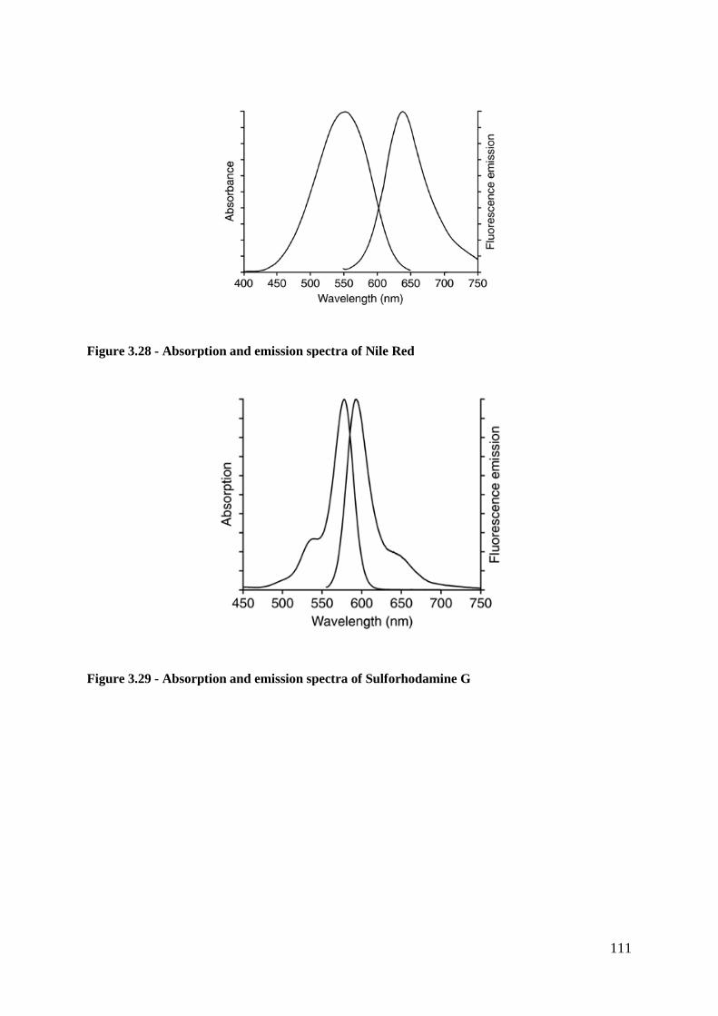
Figure 3.28 - Absorption and emission spectra of Nile Red

Figure 3.29 - Absorption and emission spectra of Sulforhodamine G

Absorption and emission spectra of Nile Red

Absorption and emission spectra of Sulforhodamine G

111

112

3.3.2 Lubricant characteristics and preparation

Two main types of lubricants were investigated in this work: single-phase (neat oil) and two-

phase (oil-in-water emulsions). This section presents all the relevant characteristics and

method of preparation for each type.

3.3.2.1 Neat oil

3.3.2.1.1 Viscometric properties

Four commercial oils representing different groups of oil were investigated in neat form,

namely an emulsifiable commercial ester oil A (i.e. a commercial ester oil containing an

emulsifier) which was also tested in emulsion form, a Group I mineral oil (which was also

used for calibration and validation of film thickness and friction measurement techniques), a

Group III mineral oil and a synthetic poly-alpha-olefin (PAO) oil. The properties of each oil

are listed in Table 3.4.

Type of oil Mineral oil,

Group I

Mineral oil,

Group III

PAO Ester oil A

S 40°C Pa s 0.056900 0.019577 0.024505 0.032495

ÃNSNhË�pÌ Pa s K-1 0.0028 0.0006 0.0010 0.0013

k W/m K 0.1400 0.1400 0.145 0.1325

α GPa-1 22 15 21 16.6

Table 3.4 - Viscometric properties of oils under test

The viscosity for each oil at 40˚C, .40°C, listed in Table 3.4 was obtained using the Stabinger

viscometer. The viscosity-temperature gradient at 40˚C, Ã[ [ËÍÎÌ, was obtained by plotting a

graph of measured viscosity against temperature for each oil tested. An ultra shear viscometer

was also used to measure viscosity at high shear rates (up to 107 s-1). The viscosity of all the

113

oils investigated remained constant with increasing shear rate, confirming that none of them

shear thin.

3.3.2.2 Oil-in-water emulsions

3.3.2.2.1 Viscometric properties

When investigating emulsions, two commercial emulsifiable ester oils were used. The two

oils had a similar formulation (same emulsifier and emulsifier concentration), with the main

difference being the viscosity. The viscosity of both oils is listed in Table 3.5.

Type of oil Emulsifiable ester oil A Emulsifiable ester oil B

S40°C , Pa s 0.032495 0.062451

Table 3.5 - Viscosity of emulsifiable oils under test

The viscosities listed in Table 3.5 were measured using the Stabinger viscometer and

correspond to the properties of the neat oil which during testing is then added to the water to

form the oil phase in the oil-in-water emulsion.

Most of the work on oil-in-water emulsions reported in this study was carried out using

emulsifiable oil A with an oil concentration of 3% and 40%. The viscosity for each oil

content was measured using a cone and plate viscometer and is given in Table 3.6.

Oil concentration

(using emulsifiable oil A)

3 % 40 %

S40°C , Pa s 0.00061 0.00394

Table 3.6 - Viscosity of emulsifiable oils in emulsion form under test

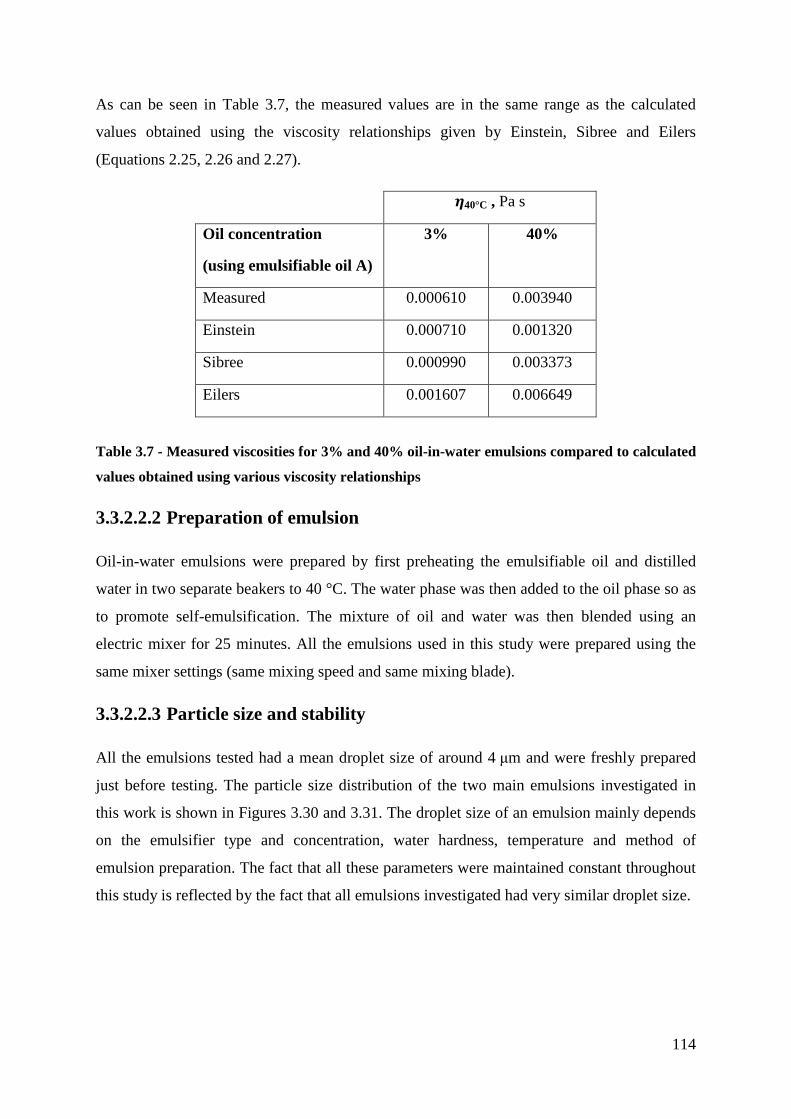
114

As can be seen in Table 3.7, the measured values are in the same range as the calculated

values obtained using the viscosity relationships given by Einstein, Sibree and Eilers

(Equations 2.25, 2.26 and 2.27).

S40°C , Pa s

Oil concentration

(using emulsifiable oil A)

3% 40%

Measured 0.000610 0.003940

Einstein 0.000710 0.001320

Sibree 0.000990 0.003373

Eilers 0.001607 0.006649

Table 3.7 - Measured viscosities for 3% and 40% oil-in-water emulsions compared to calculated

values obtained using various viscosity relationships

3.3.2.2.2 Preparation of emulsion

Oil-in-water emulsions were prepared by first preheating the emulsifiable oil and distilled

water in two separate beakers to 40 °C. The water phase was then added to the oil phase so as

to promote self-emulsification. The mixture of oil and water was then blended using an

electric mixer for 25 minutes. All the emulsions used in this study were prepared using the

same mixer settings (same mixing speed and same mixing blade).

3.3.2.2.3 Particle size and stability

All the emulsions tested had a mean droplet size of around 4 µm and were freshly prepared

just before testing. The particle size distribution of the two main emulsions investigated in

this work is shown in Figures 3.30 and 3.31. The droplet size of an emulsion mainly depends

on the emulsifier type and concentration, water hardness, temperature and method of

emulsion preparation. The fact that all these parameters were maintained constant throughout

this study is reflected by the fact that all emulsions investigated had very similar droplet size.

115

Figure 3.30 - Plot showing particle size distribution of a 3% oil-in-water emulsion, mean

particle size = 4.029µm

Figure 3.31 - Plot showing particle size distribution of a 40% oil-in-water emulsion, mean

particle size = 3.637µm

PSD measurements taken every hour showed that the droplet size of all the emulsions

investigated were stable and remained in the same range for over 2 hours. This confirms that

all the emulsions used in this study remained stable for the duration of the tests.

The stability of each emulsion was also assessed by measuring the % volume of the separated

oil phase with time. Table 3.8 shows the volume fraction of the separated oil phase together

with the mean droplet size with time for two emulsions having an oil concentration of 3% and

40%. The separated oil phase was only visible after 6 hours, whereas the tests run in this

study typically last for 30 minutes. This further confirms that all emulsions used in this study

were stable during testing.

116

Mean particle size, µm % volume of separated oil phase

Time, hrs

3% oil 40% oil 3% oil 40% oil

0 4.029 3.637 0 0

2 4.400 4.318 0 0

6 5.433 6.678 2% 4%

Table 3.8 - Mean droplet size and volume fraction for a 3% and a 40% oil-in-water emulsions

(ester oil A, same emulsifier and emulsifier concentration) with time

117

CHAPTER 4

EXPERIMENTAL RESULTS

In this section, all the experimental results and main observations together with the

corresponding test parameters are presented.

All experimental results were obtained using three main experimental techniques:

• Optical Interferometry , from which film thickness for neat oil and emulsions for

the whole range of speed investigated were obtained.

• Light Induced Fluorescence, from which visualization of the emulsion at low

speeds together with mean intensity measurements for both neat oil and emulsions

throughout the whole range of speed investigated were obtained.

• Infrared Temperature Mapping , from which temperature maps and mean

friction for both neat oil and emulsions for the whole range of speed investigated

were obtained

Results are therefore presented in three sections and then discussed in the Discussion chapter

(Chapter 5).

118

4.1 Film thickness results

4.1.1 Neat oil

Figure 4.1 shows the measured and predicted film thickness versus disc velocity of the

mineral oil under test at three different temperatures: room temperature (14 °C), 40 °C and

100 °C. The measured film thickness agrees closely with the one predicted by the Dowson-

Hamrock regression equation up to a certain speed, after which a reduction in film thickness

compared to that predicted by Equation 2.7 is obtained.

The speed at which film thickness starts to deviate from the predicted thickness varies with

temperature. The higher the viscosity of the oil, the sooner the non-linear behaviour of the oil

is experienced. The deviation in film thickness from that predicted by isothermal film

thickness equations is less pronounced at high temperatures.

Figure 4.1 - Plot showing film thickness measurement against speed for a number of tests

carried out using mineral oil at 14 °C, 40 °C and 100 °C

(Test parameters: contact: point, load: 20N, temperature: 14˚C, 40˚C, 100˚C, slide-roll ratio: idle ball, oil:

mineral, Group I)

10

100

1000

10000

0.01 0.1 1 10

Film

thic

knes

s n

m

Disc speed m s -1

predicted isothermal film thickness

experimental film thickness

14˚C

40˚C

100˚C

119

Figure 4.2 shows optical interferometric pictures of the contact which were taken during

testing to visually investigate whether the contact was starved. No inlet meniscus was visible

at any of the speeds investigated.

Figure 4.2 - Optical interference maps taken at (a) 0 m s-1 (b) 8 m s-1 (c) 10 m s-1 while a test was

run

(Test parameters: contact: point, load: 20N, temperature: 40˚C, slide-roll ratio: idle ball, oil: mineral,

Group I)

(a)

(b) (c)

120

Figure 4.3 shows the variation of viscosity with temperature. The viscosity decreases with

increasing temperature and, at high temperatures, NSNh Ï p.

Figure 4.3 - Viscosity plot showing variation of viscosity with temperature (oil: mineral, Group I)

0

0.1

0.2

0.3

0.4

0.5

0.6

0.7

0.8

0.9

0 20 40 60 80 100

SS SSPa

s

Temperature ˚C

121

Figure 4.4 shows measured film thickness values compared to a set of predicted film

thickness values obtained using the isothermal equation hiso and the thermally corrected

isothermal equation (hiso.CT) for a range of slide-roll ratios. Good agreement of the

experimental data with the thermally corrected predicted film thickness values was obtained.

As the speed increases, the experimental results agree more with the values obtained with a

correction factor for which a higher slide-roll ratio was used.

Figure 4.4 - Plot showing experimental results compared to predicted plots for a range of slide-

roll ratios using isothermal equation hiso and thermally corrected isothermal equation (hiso.CT)


Group I)

0

500

1000

1500

2000

2500

3000

3500

0 5 10 15 20 25

Film

thic

knes

s n

m

Disc speed m s -1

S=0

S=0.4S=0.8

S=1.6

S=0

S=0.4

S=0.8S=1.6

experimentalhiso (S)hiso.CT (S)

122

Figure 4.5 shows speed measurements of the idle ball obtained during testing. At low disc

speeds, the speed of the ball is the same as that of the disc, however, as the disc speed

increases further, the ball speed decreases. The slide-roll ratio is zero up to a speed of around

4.44 m s-1 and then increases as the disc speed increases further.

Figure 4.5 - Graph showing measured ball speed for each disc speed for which film thickness

measurements had previously been taken


Group I)

0.0

0.2

0.4

0.6

0.8

1.0

1.2

1.4

1.6

1.8

0.0

0.5

1.0

1.5

2.0

2.5

3.0

3.5

4.0

4.5

5.0

0 5 10 15 20

Slid

e-ro

ll ra

tio

Bal

l spe

ed m

s-1

Disc speed m s -1

ball speed slide-roll ratio

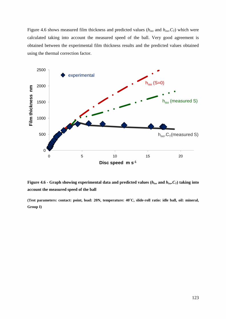
123

Figure 4.6 shows measured film thickness and predicted values (hiso and hiso.CT) which were

calculated taking into account the measured speed of the ball. Very good agreement is

obtained between the experimental film thickness results and the predicted values obtained

using the thermal correction factor.

Figure 4.6 - Graph showing experimental data and predicted values (hiso and hiso.CT) taking into

account the measured speed of the ball


Group I)

0

500

1000

1500

2000

2500

0 5 10 15 20

Film

thic

knes

s n

m

Disc speed m s -1

hiso (S=0)

hiso (measured S)

hiso.CT(measured S)

experimental

124

Figure 4.7 shows film thickness data for a set of tests which were run for a range of slide-roll

ratios, compared to the predicted film thickness values obtained using the thermal correction

factor proposed by Gupta et al. [22]. The correction factor predicts the trend fairly well, with

the extent of agreement between theory and experiment varying for different sliding/rolling

conditions.

Figure 4.7 - Graph showing experimental data obtained using group I mineral oil for a range of

slide-roll ratios compared to the corresponding predicted values obtained using the thermal

correction factor proposed by Gupta et al. [22]

(Test parameters: contact: point, load: 20N, temperature: 40˚C, slide-roll ratio: 0 – 1.9, base oil: mineral,

Group I)

0

200

400

600

800

1000

1200

1400

1600

1800

0 5 10 15 20 25

Film

thic

knes

s n

m


S=0

S=1.2

S=0.4

S=0.8

S=1.4

S=1.9

S=1.6

experimental

theoretical (Gupta et al.)

125

Figure 4.8 shows film thickness measurements obtained using different types of oil for a

range of slide-roll ratios compared to the corresponding predicted values obtained using the

thermal correction factor proposed by Gupta et al. [22]. The same trend was observed for

each type of oil, with the extent of agreement between theory and experiment varying in

accuracy for different sliding/rolling conditions.

(a)

(b)

(c)

Figure 4.8 - Graph showing experimental data obtained using (a) group III mineral oil (b) ester

oil (c) PAO for a range of slide-roll ratios compared to the corresponding predicted values

obtained using the thermal correction factor proposed by Gupta et al. [22]

(Test parameters: contact: point, load: 20N, temperature: 40˚C, slide-roll ratio: 0 – 1.9)

0

100

200

300

400

500

600

700

800

900

0 5 10 15 20 25

Film

thic

knes

s n

m


experimental


S=1.6S=1.9

S=1.2S=0.8

S=0.4

S=0

0

200

400

600

800

1000

1200

0 5 10 15 20 25

Film

thic

knes

s n

m


experimental


S=1.6

S=0.8

S=1.9

S=1.2

S=0.4

S=0

0

100

200

300

400

500

600

700

800

900

1000

0 5 10 15 20 25

Film

thic

knes

s n

m


experimental


S=0

S=0.8

S=1.6

126

Figure 4.9 shows film thickness data using group I mineral oil for a set of tests which were

run at different slide-roll ratios, compared to the predicted film thickness values obtained

using the improved thermal correction factor. Close agreement between the experimental and

predicted values is obtained throughout the whole range of slide-roll ratios.

Figure 4.9 - Graph showing experimental data obtained using group I mineral oil for a range of

slide-roll ratios compared to the corresponding predicted values obtained using the improved

thermal correction factor

(Test parameters: contact: point, load: 20N, temperature: 40˚C, slide-roll ratio: 0 – 1.9, base oil: mineral,

Group I)

0

200

400

600

800

1000

1200

1400

1600

1800

0 5 10 15 20 25

Film

thic

knes

s n

m


S=0

S=1.6S=1.9

S=1.4

S=1.2

S=0.4

S=0.8

experimental

theoretical (improved)

127

Figure 4.10 shows film thickness measurements obtained using different types of oil for a

range of slide-roll ratios compared to the corresponding predicted values obtained using the

improved thermal correction factor. Close agreement between the experimental and predicted

values is obtained throughout the whole range of slide-roll ratios.

(a)

(b)

(c)

Figure 4.10 - Graph showing experimental data obtained using (a) group III mineral oil (b)

ester oil (c) PAO for a range of slide-roll ratios compared to the corresponding predicted values

obtained using the improved thermal correction factor

(Test parameters: contact: point, load: 20N, temperature: 40˚C, slide-roll ratio: 0 – 1.9)

0

100

200

300

400

500

600

700

800

900

0 5 10 15 20 25

Film

thic

knes

s n

m


S=1.6S=1.9

S=1.2

S=0.8

S=0.4

S=0experimental


0

200

400

600

800

1000

1200

0 5 10 15 20 25

Film

thic

knes

s n

m


S=1.6

S=0.8

S=1.9

S=1.2

S=0.4

S=0experimental


0

100

200

300

400

500

600

700

800

900

1000

0 5 10 15 20 25

Film

thic

knes

s n

m


experimental

theoretical (improved)S=0

S=0.8

S=1.6

128

4.1.2 Oil-in-water emulsions

Figure 4.11 shows the film thickness measurements for a point contact obtained using a 3%

and a 40% oil-in-water emulsion compared to those obtained for neat oil and the predicted

film thickness for water. The film thickness values obtained for both emulsions at low speeds

are very similar to those obtained for neat oil (Stage I), with the film thickness measurements

obtained with the 40% oil-in-water emulsion being slightly lower than those obtained with

the 3% oil-in-water emulsion. In Stage II, both emulsions become starved, with the 3% oil-in-

water emulsion becoming more heavily starved than the 40% oil-in-water emulsion, and the

film thickness starts decreasing with increasing speed. At around 1 m s-1, the film thickness

for both emulsions starts to rise again with increasing speed. In Stage III, the film thickness

obtained for the 3% oil-in-water emulsion is very similar to that predicted for pure water

while the film thickness obtained for the 40% oil-in-water emulsion is higher than that

predicted for water but is still much lower than that measured for neat oil.

Figure 4.11 - Plot showing film thickness measurements obtained using a point contact for a 3%

and a 40% oil-in-water emulsion compared to film thickness measurements obtained for neat oil

and the predicted film thickness for water

(Test parameters: contact: point, load: 20N, temperature: 40˚C, slide-roll ratio: 0, base oil: ester A)

1

10

100

1000

10000

0.01 0.1 1 10

Film

thic

knes

s n

m


Stage I

Stage II

Stage III

neat oil

3% oil

40% oil

water (predicted)

129

Figure 4.12 shows film thickness measurements against entrainment speed obtained using a

3% oil-in-water emulsion. During the test, film thickness measurements were taken as the

speed was increased to 20 m s-1 (a), then subsequently decreased to 0.02 m s-1 (b) and then

increased again to 20 m s-1 (c). The film thickness measurements are very close in Stage I and

Stage III, however, Stage II is very unstable and seems to be dependent on whether the speed

was decreasing or increasing with time.

Figure 4.12 - Plot showing film thickness measurements using a 3% oil-in-water emulsion.

During the test, film thickness measurements were taken as the speed was (a) increased to

20 m s-1 then (b) subsequently decreased to 0.02 m s-1 and then (c) increased to 20 m s-1.


1

10

100

1000

0.01 0.1 1 10

Film

thic

knes

s nm


(b)

(a)

(c)

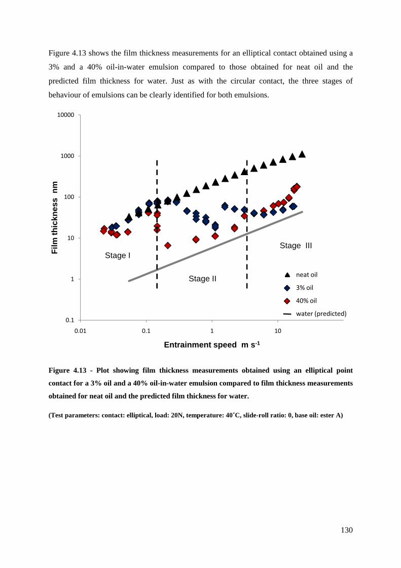
130

Figure 4.13 shows the film thickness measurements for an elliptical contact obtained using a

3% and a 40% oil-in-water emulsion compared to those obtained for neat oil and the

predicted film thickness for water. Just as with the circular contact, the three stages of

behaviour of emulsions can be clearly identified for both emulsions.

Figure 4.13 - Plot showing film thickness measurements obtained using an elliptical point

contact for a 3% oil and a 40% oil-in-water emulsion compared to film thickness measurements

obtained for neat oil and the predicted film thickness for water.

(Test parameters: contact: elliptical, load: 20N, temperature: 40˚C, slide-roll ratio: 0, base oil: ester A)

0.1

1

10

100

1000

10000

0.01 0.1 1 10

Film

thic

knes

s n

m


Stage I

Stage II

Stage III

neat oil

3% oil

40% oil

water (predicted)

131

Figure 4.14 shows the effect of oil content on film thickness. At low speeds (Stage I), the film

thickness values obtained with all emulsions are very similar to each other and to those

obtained with neat oil. The first critical speed varies for the four emulsions tested, with the

most dilute emulsion having the lowest first critical speed.

In Stage II, all the emulsions tested exhibit an unstable behaviour. Two drops in film

thickness were observed in Stage II, with the second drop being more pronounced for the

0.5% and 20% oil-in-water emulsions.

In Stage III, the film thickness increases with increasing speed. For a given entrainment

speed, a higher film thickness is obtained with the emulsion having the highest oil content.


number of oil-in-water emulsions with different oil content (0.5% oil, 3%, oil 20% oil and 40%

oil) compared to film thickness measurements obtained for neat oil and the predicted film

thickness for water. (Stage IIb is not shown in the trend lines)


1

10

100

1000

0.01 0.1 1 10

Film

thic

knes

s n

m


0.5% oil

20% oil

40% oil

3% oil

neat oil

water (predicted)

oil-in-water emulsion (different oil concentrations)

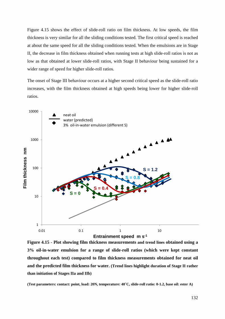
132

Figure 4.15 shows the effect of slide-roll ratio on film thickness. At low speeds, the film

thickness is very similar for all the sliding conditions tested. The first critical speed is reached

at about the same speed for all the sliding conditions tested. When the emulsions are in Stage

II, the decrease in film thickness obtained when running tests at high slide-roll ratios is not as

low as that obtained at lower slide-roll ratios, with Stage II behaviour being sustained for a

wider range of speed for higher slide-roll ratios.

The onset of Stage III behaviour occurs at a higher second critical speed as the slide-roll ratio

increases, with the film thickness obtained at high speeds being lower for higher slide-roll

ratios.


3% oil-in-water emulsion for a range of slide-roll ratios (which were kept constant

throughout each test) compared to film thickness measurements obtained for neat oil

and the predicted film thickness for water. (Trend lines highlight duration of Stage II rather

than initiation of Stages IIa and IIb)

(Test parameters: contact: point, load: 20N, temperature: 40˚C, slide-roll ratio: 0-1.2, base oil: ester A)

1

10

100

1000

10000

0.01 0.1 1 10

Film

thic

knes

s n

m


S = 0S = 0.4

S = 0.8

S = 1.2

neat oil

water (predicted)

3% oil-in-water emulsion (different S)

133

Figure 4.16 shows the effect of oil viscosity on film thickness. At low speeds, the films

formed by both emulsions are very close to those formed by the corresponding neat oils. In

Stage II, the films formed with the two emulsions are markedly different and, in Stage IIb,

the film thickness of the two emulsions start to converge, with the film thickness of the

emulsion with the more viscous oil phase decreasing with increasing speed, while the other

emulsion continues increasing.

As the emulsions enter Stage III behaviour, the film thickness obtained by both emulsions is

very similar and close to that predicted for water.

Figure 4.16 - Plot showing film thickness measurements obtained using two 3% oil-in-water

emulsions having a different oil viscosity (0.032 Pa s, 0.062 Pa s), compared to film thickness

measurements obtained using the corresponding neat oils and the predicted film thickness for

water

(Test parameters: contact: point, load: 20N, temperature: 40˚C, slide-roll ratio: 0, base oil: ester A, B)

1

10

100

1000

10000

0.01 0.1 1 10

Film

thic

knes

s n

m


S oil = 0.062 Pa s

S oil = 0.032 Pa s

neat oil

water (predicted)

3% oil-in-water emulsion (different oil phase viscosity)

134

4.2 Light Induced Fluorescence

4.2.1 Visualization of oil-in-water emulsions in EHD contacts

Figures 4.17 and 4.18 show a series of video images of the contact area in a point and

elliptical contact obtained using LIF at low speed (0.03 m s-1).

As the 3% oil-in-water emulsion approaches the inlet (right hand side), the oil droplets are

preferentially drawn into the conjunction while most of the water is squeezed out, creating a

pool, mainly of oil, at the inlet. The region of contact appears to be less intense than the inlet

region while the outlet region appears to be dark, with some oil droplets flowing in reverse

direction.

Figure 4.17 - Snapshots of contact region in a point contact obtained using LIF at 0.03 m s-1

(Stage I) (camera gain is varied when moving along the contact to account for variations in

intensity along the contact) (lens objective: x10)


cavitated region contact phase inversion at

inlet

reverse flow oil droplets

135

Figure 4.18 - Snapshots of contact region in an elliptical contact obtained using LIF at 0.03 m s-1

(Stage I) (camera gain is varied when moving along the contact to account for variations in

intensity along the contact) (lens objective: x10)


phase inversion cavitated region

oil droplets contact

136

Figure 4.19 shows video images of the whole contact region in a (a) point and (b) elliptical

contact at 0.03 m s-1 (Stage I). For both contacts, not all the oil at the inlet is drawn into the

contact; a considerable amount of it just goes around the contact and eventually rejoins the

emulsion as oil droplets.

(a)

(b)

Figure 4.19 - Snapshots of whole contact region in a (a) point and (b) elliptical contact obtained

using LIF at 0.03 m s-1 (Stage I) (lens objective: x3) – Side flow can be clearly observed in the

point contact. The elliptical contact was bigger than the field of view of the camera, however,

when looking through the microscope, the presence of side flow was verified.

(Test parameters: contact: point, elliptical, load: 20N, temperature: 40˚C, slide-roll ratio: 0, base oil:

ester A)

137

Figure 4.20 shows the measured pool distance together with the corresponding calculated

critical inlet meniscus distance (obtained using starved EHL theory for neat oil, Equation

2.11) for each of the speeds investigated. In Stage I, the oil dominated pool is quite stable and

greater than the critical inlet meniscus and decreases roughly linearly with increasing speed.

As the emulsion enters Stage II, the pool becomes smaller than the critical inlet meniscus and

much more unstable and continues to decrease until it completely disappears.

Figure 4.20 - Plot showing measured pool size together with the corresponding calculated

critical inlet meniscus (obtained using classic EHL theory for neat oil) against speed.


0

50

100

150

200

250

300

350

400

450

500

0.01 0.1 1

Poo

l dis

tanc

e

�� m


Stage I

Stage II

critical inlet distance(Hamrock and Dowson)

measured inlet distance

138

Figures 4.21 and 4.22 show video images of the inlet region of the point and elliptical contact

respectively at a number of speeds in all the three stages of behaviour of the 3% oil-in-water

emulsion. The oil pool in the inlet region (right hand side) decreases with increasing speed

until, in Stage II, it disappears. Once the pool disappears, very little is seen in the inlet region.

When the gain of the camera was considerably increased, small droplets of approximately the

same size as that of the bulk emulsion were observed in the contact region, with the

occasional droplet going in the contact.

Figure 4.21 - Snapshots of the inlet region of the point contact at a number of speeds in all the

three stages of behaviour of the 3% oil-in-water emulsion. (The images in Stage III were taken

using a higher gain camera setting.) (lens objective: x10)


139

Figure 4.22 - Snapshots of the inlet region of the elliptical contact at a number of speeds in all

the three stages of behaviour of the 3% oil-in-water emulsion. (The images in Stage III were

taken using a higher gain camera setting.) (lens objective: x10)


140

Figure 4.23 shows the measured pool size of the elliptical contact against speed. In Stage I,

the oil dominated pool is quite stable and decreases roughly linearly with increasing speed.

As the emulsion enters Stage II, the pool continues to decrease until it completely disappears.

Figure 4.23 - Plot showing measured pool size of the elliptical contact against speed


0

100

200

300

400

500

600

700

0.01 0.1 1

Poo

l dis

tanc

e

�� m


Stage I(h emulsion ≈ h neat oil)

Stage II(h emulsion< h neat oil)

141

Figure 4.24 shows a video image of the inlet region of an elliptical contact at 0.08 m s-1.

Three types of droplet behaviour were identified. Penetration droplets join the oil pool,

reverse droplets follow the water flow and are rejected (reverse droplets) while stay droplets

remain in the same place without moving.

Figure 4.24 - Snapshot of inlet region of elliptical contact at 0.08 m s-1. Three types of droplets

can be clearly identified.


reverse droplets

penetration droplets

stay droplets

142

Figure 4.25 shows video images of the point contact region obtained using a 40% oil-in-water

emulsion at 0.02 m s-1. An unstable pool can be identified, with water being squeezed out of

the contact.

Figure 4.25 - Snapshots of point contact region obtained using 40% oil-in-water emulsions at

0.02 m s-1 (Stage I) (camera gain is varied when moving along the contact to account for

variations in intensity along the contact) (lens objective: x10)


Figure 4.26 shows video images of the point contact region obtained using a 40% oil-in-water

emulsion at 0.08 m s-1. The oil dominated pool is not visible any more. No water can be seen

being squeezed out of the contact and no real distinction between the bulk emulsion and inlet

region could be seen.

Figure 4.26 - Snapshots of point contact region obtained using a 40% oil-in-water emulsion at

0.08 m s-1 (Stage I) (camera gain is varied when moving along the contact to account for



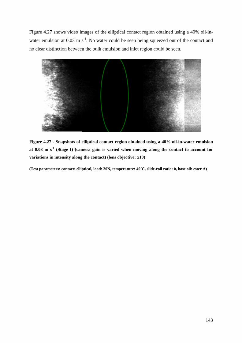
143

Figure 4.27 shows video images of the elliptical contact region obtained using a 40% oil-in-

water emulsion at 0.03 m s-1. No water could be seen being squeezed out of the contact and

no clear distinction between the bulk emulsion and inlet region could be seen.

Figure 4.27 - Snapshots of elliptical contact region obtained using a 40% oil-in-water emulsion

at 0.03 m s-1 (Stage I) (camera gain is varied when moving along the contact to account for



144

4.2.2 Mean intensity measurements

Figures 4.28 (a) and (b) show the variation in intensity with film thickness using the oil-

soluble dye (dissolved in neat oil) and the water-soluble dye (dissolved in pure water). The

intensity variation is negligible up to a film thickness of about 500 nm for both dyes used.

(a)

(b)

Figure 4.28 - Plots obtained using (a) oil-soluble dye and (b) the water-soluble dye showing

intensity variation with film thickness (Note: The scale on the two graphs is very different due to the

fact that two cameras with different resolution (8-bit, 16-bit) were used.)

(Test parameters: contact: point, (a) moving (b) static, load: 20N, temperature: 40˚C, slide-roll ratio: 0)

0

50

100

150

200

250

300

0 200 400 600 800 1000 1200

Inte

nsity

gray

scal

e le

vel

Film thickness nm

0

500

1000

1500

2000

2500

3000

0 100 200 300 400 500

Inte

nsity

gray

scal

e le

vel

Film thickness nm

145

Figures 4.29 (a) and (b) show the variation in intensity with oil concentration using the oil-

soluble and the water-soluble dye. Oil concentration was varied by using a number of oil-in-

water emulsions with different oil content. The intensity is sensitive, but not uniquely related

to composition. This non-linear behaviour was only experienced when the oil was tested in

emulsion form. When neat oil or pure water was used and the dye content was varied by

varying the dye concentration rather than the oil or water content in the emulsion, a linear

relationship was obtained (dotted line).

(a)

(b)

Figure 4.29 - Plots obtained using (a) the oil-soluble dye (dissolved in the oil phase of the

emulsion) and (b) the water-soluble dye (dissolved in the water phase of the emulsion) showing

intensity variation with emulsion composition (Intensity values were obtained using 16-bit resolution

camera.)

(Test parameters: contact: point (static) load: 20N, temperature: 40˚C, slide-roll ratio: 0)

0

500

1000

1500

2000

2500

3000

0 20 40 60 80 100

Inte

nsity

gray

scal

e le

vel

oil content, %

0

1000

2000

3000

4000

5000

0 20 40 60 80 100

Inte

nsity

gray

scal

e va

lue

water content, %

146

Figure 4.30 shows images of a dyed oil droplet in water and a water droplet in dyed oil. A

ring of very high intensity can clearly be seen around the oil droplet. This effect is not

experienced when the dyed oil is the continuous phase rather than in droplet form.

(a) (b)

Figure 4.30 - Image captured by camera showing (a) a dyed oil droplet in water and (b) a water

droplet in dyed oil.

Figure 4.31 shows images of oil droplets in dyed water and dyed water droplets in oil. A very

high intensity can clearly be seen around the oil droplet (Figure 4.31 (a)). This effect is not

experienced when the dyed oil is the continuous phase (Figure 4.31 (b)) rather than in droplet

form and is less pronounced than when the dyed oil is in droplet form (Figure 4.30 (a)).

(a) (b)

Figure 4.31 - Image captured by camera showing (a) oil droplets in dyed water and (b) dyed

water droplets in oil.

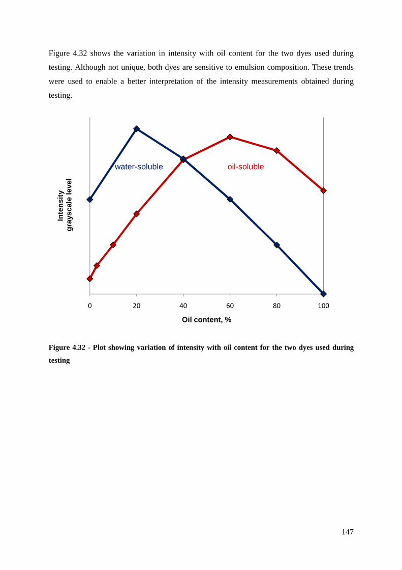
147

Figure 4.32 shows the variation in intensity with oil content for the two dyes used during

testing. Although not unique, both dyes are sensitive to emulsion composition. These trends

were used to enable a better interpretation of the intensity measurements obtained during

testing.

Figure 4.32 - Plot showing variation of intensity with oil content for the two dyes used during

testing

0

500

1000

1500

2000

2500

3000

3500

4000

4500

5000

0

10

20

30

40

50

60

70

80

0 20 40 60 80 100

Inte

nsity

gray

scal

e le

vel

Oil content, %

oil-solublewater-soluble

148

Figures 4.33 and 4.34 show the intensity measurements for a circular point contact, obtained

using a 3% and a 40% oil-in-water emulsion using an oil-soluble and water-soluble dye,

together with the intensity benchmark values for neat oil and pure water. For all the tests

carried out, a marked variation in the intensity of both dyes is obtained as the speed is

increased and transition from Stage I to Stage III occurs.

At low speeds, the intensity values obtained for the dilute emulsion with both the oil-soluble

and water-soluble dye remain relatively constant and the intensity values obtained from the

oil-soluble dye are very close to those obtained with neat oil. As the speed starts to increase,

the intensity measurements start to vary. The intensity of the oil-soluble dye decreases greatly

whereas the intensity of the water-soluble dye increases and is slightly higher than that

obtained with pure water.

Figure 4.33 - Plot showing the intensity measurements obtained when testing a 3% oil-in-water

emulsion using an oil-soluble and water-soluble dye, together with intensity benchmarks for

neat oil and pure water. (Intensity values were obtained using 16-bit resolution camera.)


0

1000

2000

3000

4000

5000

6000

1

10

100

1000

10000

0.01 0.1 1 10

Inte

nsity

gra

ysca

le

leve

l

Film

thic

knes

s n

m

Entrainment speed m s-1

film thickness, neat oil Intensity measurement, water soluble dye, 3% oil

film thickness, 3% oil Intensity measurement, oil soluble dye, 3% oil

Ipure water

Ineat oil

(h<500nm)

Stage II Stage IIIStage I

149

The intensity values obtained with the concentrated emulsion at low speeds are relatively

constant and the values obtained with the oil-soluble dye are very close to the intensity

benchmark for neat oil. The water intensity values were higher than the benchmark intensity

value for water throughout the whole range of speeds investigated.

Figure 4.34 - Plot showing the intensity measurements obtained when testing a 40% oil-in-water


neat oil and pure water. (Intensity values were obtained using 16-bit resolution camera.)


0

1000

2000

3000

4000

5000

6000

7000

8000

1

10

100

1000

10000

0.01 0.1 1 10

Inte

nsi

ty g

ray

sca

le l

ev

el

Film

thic

knes

s n

m

Entrainment speed ms -1

film thickness, neat oil intensity measurement, water soluble dye, 40% oil

film thickness, 40% oil intensity measurement, oil soluble dye, 40% oil

I pure water

I neat oil

(h<500nm)


150

Figures 4.35 and 4.36 show the intensity measurements for an elliptical contact obtained

using a 3% and a 40% oil-in-water emulsion using an oil-soluble and water-soluble dye. The

trends look similar to those obtained with point contacts. For all the tests carried out, a

marked variation in the intensity of both water-soluble and oil-soluble dye is obtained as the

speed is increased and transition from Stage I to Stage III occurs.

Figure 4.35 - Plot showing the intensity measurements obtained when testing 3% oil-in-water


neat oil and pure water (Intensity values were obtained using 16-bit resolution camera.)


1000

1200

1400

1600

1800

2000

2200

2400

2600

2800

3000

1

10

100

1000

10000

0.01 0.1 1 10In

tens

ity g

rays

cale

leve

l

Film

thic

knes

s n

m





151

Figure 4.36 - Plot showing the intensity measurements obtained when testing 40% oil-in-water


neat oil and pure water (Intensity values were obtained using 16-bit resolution camera.)


0

1000

2000

3000

4000

5000

6000

0.1

1

10

100

1000

10000

0.01 0.1 1 10

Inte

nsity

gra

ysca

le le

vel

Film

thic

knes

s n

m





152

4.3 Infrared temperature and friction measurements

4.3.1 Neat oil

Figures 4.37 (a), (b), (c) and (d) show an example of all the maps obtained with the infrared

temperature mapping technique. The inlet is at the front right of the maps and sliding is in the

direction of −y.

a) Temperature rise map of disc surface (ºC)

b) Temperature rise map of ball surface (ºC)

c) Total heat flux map (W/m2) d) Shear stress map (Pa)

Figure 4.37 - Maps for contact lubricated with mineral oil

(Test parameters: contact: point, load: 20N, temperature: 40˚C, slide-roll ratio: 0.8, base oil: mineral,

Group I, entrainment speed: 4.34 m s-1)

0

500

0

500

0

5

10

15

20

x (µm)y (µm) 0

5

10

15

20

0

500

0

500

-10

0

10

20

x (µm)y (µm) 0

5

10

15

20

25

0

500200

400600

0

2

4

6

x 107

x (µm)y (µm) 0

1

2

3

4

5

6

7

x 107

0

500200

400600

0

5

10

15

20

x 106

x (µm)y (µm) 0

0.5

1

1.5

2

x 107

153

Figures 4.38 (a) and (b) show the heat flux along the contact for a low speed (0.412 m s-1)

and a high speed (11.65 m s-1) calculated using the original approach (i.e. assuming all heat

generated within the contact is conducted to the bounding surfaces) and the modified

approach which takes convection into account.

At low speed, the calculated heat flux profiles obtained using both approaches are identical.

At high speed, the shape of the profile differs mostly in the central part of the contact, where

the highest temperatures are experienced. As the exit region is approached, the heat flux

drops below zero.

(a)

(b)

Figure 4.38 - Plot showing the calculated heat flux along the contact at (a) 0.412 m s-1 and (b)

11.65 m s-1 obtained using the original equation (Equation 3.5) and the corrected equation

(Equation 3.12) which takes into account convection

(Test parameters: contact: point, load: 20N, temperature: 40˚C, slide-roll ratio: 0.8, base oil: ester A)

-2.0E+06

0.0E+00

2.0E+06

4.0E+06

6.0E+06

8.0E+06

1.0E+07

1.2E+07

1.4E+07

0 200 400 600

Hea

t flu

x W

/m2

Distance µm

not corrected

corrected (for convection)

-2.00E+07

0.00E+00

2.00E+07

4.00E+07

6.00E+07

8.00E+07

1.00E+08

1.20E+08

0 200 400 600 800

Hea

t flu

x W

/m2

Distance ��m

not corrected


154

Figure 4.39 shows the overall friction plot obtained using shear stress values obtained from

the original and corrected heat flux maps for the same load and sliding conditions used to

obtain Figures 4.38 (a) and (b). The friction values are very similar to each other throughout

the whole range of speed investigated.

Figure 4.39 - Friction plot obtained using shear stress values obtained from the original and

corrected heat flux maps


0

0.005

0.01

0.015

0.02

0.025

0.1 1 10 100

Fric

tion

coef

ficie

nt


not corrected


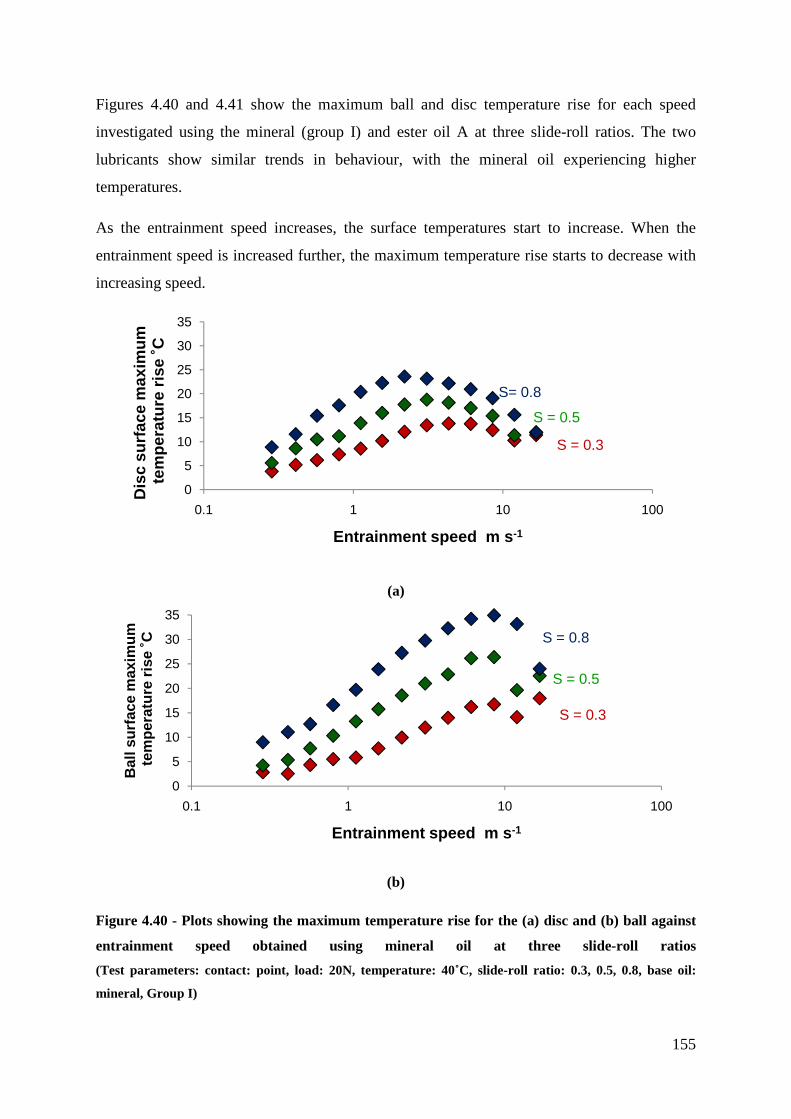
155

Figures 4.40 and 4.41 show the maximum ball and disc temperature rise for each speed

investigated using the mineral (group I) and ester oil A at three slide-roll ratios. The two

lubricants show similar trends in behaviour, with the mineral oil experiencing higher

temperatures.

As the entrainment speed increases, the surface temperatures start to increase. When the

entrainment speed is increased further, the maximum temperature rise starts to decrease with

increasing speed.

(a)

(b)

Figure 4.40 - Plots showing the maximum temperature rise for the (a) disc and (b) ball against

entrainment speed obtained using mineral oil at three slide-roll ratios

(Test parameters: contact: point, load: 20N, temperature: 40˚C, slide-roll ratio: 0.3, 0.5, 0.8, base oil:

mineral, Group I)

0

5

10

15

20

25

30

35

0.1 1 10 100

Dis

c su

rfac

e m

axim

umte

mpe

ratu

re r

ise

˚C


S= 0.8

S = 0.5

S = 0.3

0

5

10

15

20

25

30

35

0.1 1 10 100

Bal

l sur

face

max

imum

tem

pera

ture

ris

e ˚C


S = 0.8

S = 0.5

S = 0.3

156

At low entrainment speeds, the surface temperatures of the ball and disc are reasonably close

to each other, with the disc surface being slightly hotter than the ball surface. As the speed

increases, the surface temperatures start to diverge, with the ball surface becoming

considerably hotter than the disc surface, particularly for the higher slide-roll ratios.

(a)

(b)

Figure 4.41 - Plots showing the maximum temperature rise for the (a) disc and (b) ball against

entrainment speed obtained using ester oil at three slide-roll ratios


ester A)

0

5

10

15

20

25

0.1 1 10 100

Dis

c su

rfac

e m

axim

umte

mpe

ratu

re r

ise

˚C


S = 0.8

S= 0.5

S = 0.3

0

5

10

15

20

25

0.1 1 10 100

Bal

l sur

face

max

imum

tepm

pera

ture

ris

e ˚C


S = 0.8

S = 0.5

S = 0.3

157

Figures 4.42 and 4.43 show the traction coefficient for mineral oil and ester oil respectively,

using three slide-roll ratios. Both oils exhibit similar trends in behaviour.

At low entrainment speeds, the traction coefficient remains constant for all slide-roll ratios

tested. As the speed is further increased, the traction coefficient starts to decrease with

increasing speed. The reduction in friction initiates at lower entrainment speeds and is more

pronounced for higher slide-roll ratios.

Figure 4.42 - Plots showing average traction coefficient against entrainment speed obtained

using mineral oil at three slide-roll ratios


mineral, Group I)

Figure 4.43 - Plots showing average traction coefficient against entrainment speed obtained

using ester oil at three slide-roll ratios


ester A)

0

0.01

0.02

0.03

0.04

0.05

0.06

0.1 1 10 100

Trac

tion

coef

ficie

nt


S = 0.8S = 0.5

S = 0.3

0

0.01

0.02

0.03

0.04

0.1 1 10 100

Trac

tion

coef

ficie

nt


S = 0.8

S = 0.5

S = 0.3

158

4.3.2 Oil-in-water emulsions

Figure 4.44 shows the measured maximum surface temperature rise for the 3% oil-in-water

emulsion and neat oil as the speed is increased up to 20 m s-1. The temperature rise obtained

with the dilute emulsion is significantly lower than that obtained with neat oil.


emulsion and neat oil for speeds of up to 20 m s-1


0

5

10

15

20

0.1 1 10 100

Dis

c su

rfac

e m

axim

umte

mpe

ratu

re r

ise

˚C


neat oil

3% oil

159

Figure 4.45 shows the calculated friction for 3% oil-in-water emulsion and neat oil (at a slide-

roll ratio of 0.8) as the speed is increased up to 20 m s-1.

In Stage II, the friction value obtained for the 3% oil-in-water emulsion is initially very close

to that obtained with neat oil. As the speed is further increased (but still in Stage II), the

friction coefficient starts to decrease, despite the decrease in film thickness. In Stage III, the

friction coefficient obtained with the 3% oil-in-water emulsion is reasonably stable and much

lower than that obtained with neat oil, even though the films formed by the emulsions are

much thinner than those formed by neat oil.

Figure 4.45 - Plot showing the mean traction coefficient (calculated from measured temperature

rise) for 3% oil-in-water emulsion and neat oil for speeds of up to 20 m s-1.


0.01

0.1

1

10

100

0.001

0.01

0.1

1

0.01 0.1 1 10

Film

thic

knes

s n

m

Trac

tion

coef

ficie

nt


neat oil (�) 3% oil (�)

3% oil (h) neat oil (h)

Stage I

Stage II

Stage III

160

Figure 4.46 shows the measured maximum surface temperature rise for the 40% oil-in-water

emulsion and neat oil (at a slide-roll ratio of 0.8) as the speed is increased up to 20 m s-1. The

temperature rise obtained with the concentrated emulsion is significantly lower than that

obtained with neat oil.


emulsion and neat oil for speeds of up to 20 m s-1


0

5

10

15

20

0.1 1 10 100

Dis

c su

rfac

e m

axim

umte

mpe

ratu

re r

ise

˚C


neat oil

40% oil

161

Figure 4.47 shows the calculated friction for 40% oil-in-water emulsion and neat oil as the

speed is increased up to 20 m s-1.

Friction values are lower than those obtained with neat oil from the very start of Stage II and

continue decreasing gradually with increasing speed. In Stage III, the friction coefficient

decreases further and is significantly lower than that obtained with neat oil.

Figure 4.47 - Plot showing the mean traction coefficient (calculated from measured temperature

rise) for 40% oil-in-water emulsion and neat oil for speeds of up to 20 m s-1.


0.01

0.1

1

10

100

0.001

0.01

0.1

1

0.01 0.1 1 10

Film

thic

knes

s n

m

Trac

tion

coef

ficie

nt


Stage I

Stage II

Stage III

neat oil (µ) 40% oil (µ)

40% oil (h) neat oil (h)

162

CHAPTER 5

DISCUSSION

5.1 Behaviour of single-phase lubricants at high speed

5.1.1 Introduction

In this chapter, the behaviour of neat oil at high speeds is investigated. Understanding the

behaviour of the single-phase lubricants at high speeds is essential before proceeding with the

investigation of two-phase lubrication. Not much experimental testing has been done by other

researchers in the range of speed of interest (speeds higher than 5 m s-1) so, in this section,

film thickness measurements, friction and temperature maps obtained using neat oil at high

speeds are discussed.

5.1.2 Film thickness

5.1.2.1 Introduction

When investigating film formation, two sets of tests were carried out. In the preliminary

phase, tests were run in tractive rolling and film thickness measurements and visual

observations were employed to better understand the behaviour of film thickness at high

speeds by identifying which of the factors discussed in Chapter 2 (starvation, inlet shear

heating and/or sliding) are present at high speeds. The second sets of tests were run in

controlled sliding conditions so that the factors which were previously found to be affecting

film thickness at high speeds could be investigated in greater detail.

163

5.1.2.2 Preliminary Testing

5.1.2.2.1 Film thickness results and observations

Figure 4.1 shows (in log vs log form) the measured and predicted film thickness (using

Equation 2.7) versus disc velocity of the mineral oil under test at three different temperatures:

room temperature (14 °C), 40 °C and 100 °C. The measured film thickness agrees closely

with the one predicted by the Dowson-Hamrock regression equation up to a certain speed,

after which a reduction in film thickness compared to that predicted by Equation 2.7 is

obtained.

The speed at which film thickness starts to deviate from the predicted thickness varies with

temperature, suggesting that this behaviour is strongly linked to the viscosity of the oil and

the temperature at which the test is run. The higher the viscosity of the oil, the sooner the

non-linear behaviour of the oil is experienced. Also, it seems that, when testing at high

temperatures, the behaviour of the oil deviates much less even at high speeds.

5.1.2.2.2 Identifying the dominant factor affecting film thi ckness behaviour

at high speeds

As mentioned in Chapter 2, the factors which may contribute to this reduction in film

thickness below the values predicted by the isothermal regression equations are starvation,

shear thinning, sliding and thermal effects. In this section, an attempt will be made to explain

the behaviour of film thickness at high speeds in terms of the factors which could be causing

this reduction in film thickness (i.e. starvation, shear thinning, sliding and/or inlet shear

heating) to try and determine which of these mainly contribute to such behaviour. This

analysis was mainly focused on the results obtained at 40 °C.

5.1.2.2.2.1 Starvation

The results shown in Figure 4.1 could in principle be explained by starvation since the

reduction of the film thickness below the theoretical value occurs at a lower speed for the

higher viscosities. The more viscous the oil is, the more difficult it is for the oil to replenish

the oil pool as the speed increases. The results in Figure 4.1 agree with this. However, when

164

starvation ensues, the fall in film thickness is usually quite sharp. This does not appear to be

the case for the results obtained.

Optical interferometric pictures of the contact which were taken during testing to try and

visually investigate what is actually occurring at the contact showed no clear signs of

starvation (Figure 4.2). A change in film shape was also observed as the speed increased, as

previously observed in [93]. No inlet meniscus was visible; therefore experimental evidence

did not suggest the presence of starvation. Furthermore, an adequate supply of lubricant was

supplied to the contact. All these factors make it highly improbable that starvation is the

dominant factor affecting the behaviour of film thickness at high speeds.

5.1.2.2.2.2 Shear Thinning

Shear thinning could also explain the behaviour of the oil at high speeds. If the oil is non-

Newtonian at the shear rates reached at the contact, the effective viscosity at the inlet of the

contact will drop with increasing speed, resulting in a reduction in film thickness compared to

the ones predicted by the Newtonian Dowson-Hamrock equation. Tests were performed using

an ultra high shear viscometer for a range of temperatures which were calculated to be

reached at the contact inlet during testing (see next section). The lubricant remained

Newtonian throughout; hence the possibility of explaining film thickness behaviour at high

speeds by shear thinning was ruled out.

5.1.2.2.2.3 Inlet Shear Heating

Inlet shear heating could also explain the results shown in Figure 4.1. At high speeds, the

very high lubricant shear rates created at the contact inlet cause the inlet temperature to rise,

causing a drop in inlet viscosity, thereby reducing film thickness. Shear heating would also

explain why the reduction in film thickness compared to the predicted ones was much lower

when the test was run at a temperature of 100°C (see Figure 4.1). As can be seen from Figure

4.3, at high temperatures, [ [ Ï 0. Ð � �

[ [

also declines with increasing temperature, having

the value 5.0 × 10-2 °C-1 at 40 °C but only 2.8 × 10-2 °C-1 at 100 °C. The consequent fractional

reduction in film thickness with temperature will vary as β0.67 and so also declines as the

temperature increases, resulting in a lower effect of inlet shear on film thickness at higher

temperatures even though the temperature rise in the inlet may still be appreciable.

165

The corresponding effective inlet viscosity for each experimental film thickness value was

calculated and, from the viscosity-temperature behaviour of the lubricant, the effective

temperature at the inlet was derived. At a disc speed of 19 m s-1, the effective viscosity

dropped to 0.0125 Pa s, corresponding to an inlet temperature of 84 °C. (Note: The

entrainment speed used to calculate the inlet temperature was obtained using the disc speed

and the measured ball speed (i.e. sliding was taken into account).

The thermal reduction factor proposed by Gupta et al. [22] was applied to the theoretical

isothermal film thickness predicted by Equation 2.7 for the conditions present during testing.

Different values of slide-roll ratios were used to obtain a number of predicted values under

different degrees of sliding (Figure 4.4).

As can be seen in Figure 4.4, there is good agreement of the experimental data with the

theoretical values obtained using the isothermal film thickness calculated by the Dowson-

Hamrock equation (Equation 2.7) multiplied by the correction factor (hiso× CT). As the speed

increases, the experimental results seem to agree more with the values obtained with a

correction factor for which a higher slide-roll ratio was used. The above results therefore

suggest that some sliding is occurring and that this is increasing with increasing speed.

5.1.2.2.2.4 Sliding

If sliding is experienced during testing, the entrainment speed would be lower than that for

pure rolling (which was the assumed condition at the contact) and additional shearing

resulting from sliding of the two surfaces would be experienced at the contact, resulting in a

further reduction in film thickness.

Speed measurements of the idle ball obtained during testing are shown in Figure 4.5. At low

disc speeds, the speed of the ball is the same as that of the disc, confirming that there is pure

rolling motion up to a speed of about 4.4 m s-1. As the disc speed increases further, the ball

speed decreases, and the ball starts to slip. The slide-roll ratio is zero (i.e. no sliding is

occurring) up to a speed of about 4.44 m s-1 and then increases as the disc speed increases

further (Figure 4.5).

166

5.1.2.2.3 Predicted film thickness taking into account sliding and inlet shear

heating

The corresponding ball speeds for each disc speed at which film thickness measurements

were previously taken were used to calculate the respective entrainment speed and slide-roll

ratio. This data was then used to calculate the thermal correction factor and the isothermal

film thickness, from which the predicted film thicknesses were obtained (hiso × CT) (Figure

4.6).

As can be seen in Figure 4.6, when the actual velocity of the ball (and therefore the condition

of sliding) was taken into account and a thermal correction factor was applied, the agreement

of the experimental data with the predicted values obtained using the isothermal film

thickness equation multiplied by the thermal correction factor (hiso × CT (measured S)) is very

close to the experimental results obtained.

Predicted values were in agreement with the experimental values within an error of 8% – this

% error includes the error coming from the values of the speed of the ball which were

calculated from the approximate sine waves obtained on the CRO screen therefore the

agreement of the predicted values with the experimental ones is remarkable. This close

agreement strongly suggests that the behaviour of the single-phase lubricant at high speeds is

best described by the effect of inlet shear heating at the observed sliding speeds.

5.1.2.3 Further testing to assess shear heating theory

In Section 5.1.2.2, it was determined that the behaviour of the single-phase lubricant at high

speeds is best described by the effect of inlet shear heating. In this section, further testing was

done to assess the accuracy of the inlet shear heating theory at different sliding conditions

and for different types of oil.

5.1.2.3.1 Tests run at controlled sliding conditions

In the preliminary phase, tests were run in tractive rolling where it was found that the ball

starts to slip as the speed increases and, as a result of this, the slide-roll ratio varied

throughout the test. When assessing the accuracy of the shear heating theory, it was felt

important that tests were carried out using a fixed slide-roll ratio throughout the test. This was

167

achieved by driving the ball and disc using two separate motors, thereby allowing tests to be

run in pure rolling (disc speed = ball speed) and in sliding conditions (disc speed Ñ ball

speed), with each condition being kept constant throughout the whole test. Having a

controlled slide-roll ratio throughout the test eliminates the source of error coming from the

calculation of the speed of the ball, thereby allowing the accuracy of the correction factor to

be established.

Figure 4.7 shows film thickness data for a set of tests which were run for a range of slide-roll

ratios, which were kept constant throughout each test, compared to the predicted film

thickness values obtained using the thermal correction factor proposed by Gupta et al.[22].

Although the correction factor predicts the trend fairly well, the extent of the agreement

between theory and experiment varies for different sliding/rolling conditions. The correction

factor seems to overestimate the effect of high entrainment speed (experimental film

thickness values higher than the thermally corrected predicted ones at pure rolling) and

underestimates the effect of sliding (experimental film thickness values lower than the

thermally corrected ones predicted at high sliding).

One possible explanation for this discrepancy is that the theory (Wilson et al. [19], Cheng et

al. [20] used to derive the correction factor used two steel surfaces while in these experiments

two different surfaces, one more conductive than the other, were used. Another possible

explanation is that the inlet shear correction factor [22], which was derived semi-empirically

for a specific oil, does not explicitly take into account oil properties such as heat capacity,

thermal expansivity and compressibility of the oil, which can vary for different types of oil.

This is addressed further in the next section.

Although at slide-roll ratios of 0 - 1.2 the difference between the predicted data and the

experimental ones is significant, the agreement of the predicted values with the experimental

ones is very close for slide-roll ratios of 1.4 and 1.6. This explains why, in the preliminary

testing, the film thickess data obtained during a test run in tractive rolling and the predicted

data (which was corrected to account for the speed of the ball which changed during the test)

were in very close agreement since, during the test, at high disc speeds, slide-roll ratios of 1.3

and 1.5 were experienced.

168

5.1.2.3.2 Tests run using different types of oil

The tests run in the preliminary phase were all carried out using mineral oil. Further tests

using different types of oil having different viscometric properties were carried out to see

whether thermal effects are always the dominant factor in high speed conditions. These tests

also establish whether the thermal correction factor used in this work could be used for

different types of oil.

Figures 4.8 (a) (b) and (c) show film thickness measurements for a set of tests which were run

for a range of slide-roll ratios compared to the predicted film thickness values obtained using

the thermal correction factor proposed by Gupta et al. [22]. The same trend was observed for

each type of oil, confirming that thermal effects were the dominant factor affecting film

thickness in high speed conditions.

5.1.2.3.3 Improving correction factor

Now that a whole set of film thickness data for a range of slide-roll ratios are available, an

attempt was made to improve the correction factor in order to improve the agreement of the

predicted values to the experimental ones for each type of oil tested. This was done by

modifiying the coefficients a, b, c and d of the correction factor proposed by Gupta et al. [22]

for each type of oil tested:

ih � W�WR.XTca �p.�XW5 �W5��Z Equation 5.1

Figure 4.9 shows a comparison between the predicted data obtained using the improved

correction factor and the experimental data obtained on the rig using a group I mineral oil at

various degrees of sliding. The improved factor gives a better fit throughout the whole range

of slide-roll ratios, with an error of less than 10 % for entrainment speeds higher than 1 m s-1.

A similar fit was done for each type of oil tested to see whether this improved thermal factor

is as effective for different types of oil tested. The coefficients which give better agreement

with the experimental data (Figures 4.10 (a), (b) and (c)) differ slightly for each type of oil

and are shown in Table 5.1. As suggested earlier, the variations in the coefficients probably

reflect differences in the physical properties of the individual oils.

169

a b c d

Gupta et al. (original coefficients) 0.21 2.2 0.83 0.64

Mineral oil, Group I 0.12 2.8 2.0 0.54

Mineral oil, Group III 0.12 2.5 1.7 0.54

PAO 0.18 2.2 1.8 0.54

Ester Oil 0.18 1.6 2.2 0.44

5.1.2.4 Summary of achievements

This section analysed the major factors which could influence film thickness of

elastohydrodynamic contacts at very high speeds. Preliminary results were used to try and

explain film thickness behaviour in terms of starvation and thermal effects (sliding and inlet

shear heating). After both possible explanations for the reduction in film thickness at high

speeds were compared with experimental data and observations, it was concluded that the

effect which best describes the behaviour of film thickness at very high speeds is inlet shear

heating.

The accuracy of the inlet shear heating theory has also been assessed by running experiments

at controlled sliding conditions and using different types of oil up to entrainment speeds of

20 m s-1. It was found that the thermal correction factor predicts the trend of film thickness

behaviour well for all of the oils tested, and the agreement of the predicted values with the

experimental ones is very close for certain slide-roll ratios. The experimental data were also

used to obtain improved empirical coefficients for the correction factor for different types of

oil.

Table 5.1 - Coefficients used for each type of oil tested to provide best agreement with experimental data

170

5.1.3 Friction


IR temperature mapping was used to obtain surface temperature maps together with shear

stress maps and overall friction at the contact. The main aim of this section was to investigate

the friction properties of neat oil at high speeds which could then be directly compared to

friction results obtained using oil-in-water emulsions in Section 5.2.1 to see how they differ.

Using the IR technique described in Chapter 3.2, temperature maps were obtained for the ball

and disc surface at all the speeds investigated, from which heat flux and shear stress maps

were calculated. An example of all the maps obtained with this technique are shown in

Figures 4.37 (a), (b), (c) and (d). Figures 4.37 (a) and (b) show the disc and ball surface

temperature rise. In both maps, the temperature rise increases rapidly to a maximum within

the contact and then falls slowly in the exit region. The temperature of the sapphire disc

surface falls more slowly than that of the steel ball. This is due to the fact that the thermal

diffusivity of sapphire is lower than that of steel (see Table 3.1).

Weak interference fringes are visible on the temperature map of the ball surface. This weak

interference occurs due to the high refractive index of the sapphire disc (which is uncoated

during the measurement of the ball surface temperature) and can be used to locate the centre

of the contact. Interference fringes are not visible on the temperature maps of the disc as the

chromium coating used when measuring the temperature of the disc is completely reflective.

Using the moving heat source theory (Section 3.2.1.3.1.1.3), the two temperature rise maps

were then converted into maps of heat flux (Figure 4.37 (c)). These were in turn used to

calculate the lubricant film shear stress map (Figure 4.37 (d)), and, by integrating the shear

stress over the area of the contact and dividing by the applied load, the overall friction

coefficient was obtained.

5.1.3.2 Effect of convection on shear stress distribution and friction at high

speeds

In Section 3.2.1.3.1.4.1 it was argued that, at high speeds, a significant part of the heat

generated by shearing could be convected along the film rather than conducted to the ball and

171

disc surfaces, possibly compromising one of the main assumptions of the technique. To take

convection into account, two additional terms which are a function of the measured surface

temperatures and the convection to conduction ratio were added to the equation used to

calculate the heat flux (Equation 3.12).

Figures 4.38 (a) and (b) show the heat flux along the contact for a low speed (0.412 m s-1)

and a high speed (11.65 m s-1) calculated using the original equation (Equation 3.5) and the

modified equation (Equation 3.12) which takes convection into account.

At low speed, the calculated heat flux profiles obtained using the two equations are identical.

This is because, at low speeds, the conduction to convection ratio is high hence the

convection terms added to Equation 3.12 are negligible. At high speed, however, some

differences can be seen. The shape of the profile differs mostly in the central part of the

contact, where the highest temperatures are experienced. As the exit region is approached, the

heat flux drops slightly below zero. This could be due to the fact that, at this position, the

surfaces are colder than the oil, resulting in a negative heat flux.

Since the main use of this technique in this study is to obtain the overall friction, the effect of

convection on the overall friction was assessed. Figure 4.39 shows the overall friction plot

obtained using shear stress values obtained from the original and corrected heat flux maps for

the same load and sliding conditions used to obtain Figures 4.38 (a) and (b).

The friction values are very similar to each other throughout the whole range of speed

investigated. This shows that, although convection losses affect the shape of the calculated

shear stress distribution, the integral of the shear stress is little affected.

This can be explained as, when calculating friction, the contact is treated as a whole rather

than as an array of elements as is done when mapping the shear stress. The ratio of

convection to conduction is calculated using a value of B (defined in Section 3.2) that is equal

to the diameter of the contact (256 µm). This gives a ratio of conduction to convection that is

high throughout the whole range of speed investigated.

Hence, at high speeds, convection losses affect the shape of the calculated shear stress

distribution, however, the overall friction, which is the main characteristic of interest in this

section, is largely unaffected.

172

5.1.3.3 Temperature maps and friction results

5.1.3.3.1 Temperature maps

Temperature maps of the ball and disc surfaces were obtained for a range of speeds and

sliding conditions using a group I mineral oil and an ester oil. The maximum ball and disc

temperature rise for each speed investigated using the mineral and ester oil are shown in

Figures 4.40 and 4.41 respectively. The two lubricants show similar trends in behaviour.

Higher temperatures are experienced with the mineral oil. This is because this oil is more

viscous than the ester oil, resulting in more shearing of the lubricant occurring at the contact.

As the entrainment speed (and sliding speed, ∆U) increases, the surface temperatures start to

increase. This behaviour is expected as, the higher the sliding speed, the more shearing of the

lubricant occurs and more heat is generated within the contact. This also explains why the

surface temperatures for a given speed depends on the slide-roll ratio used during testing

where, the higher the slide-roll ratio, the higher the temperature rise experienced within the

contact.

As the entrainment speed is further increased, the maximum temperature rise starts to

decrease with increasing speed. This could be partly due to the fact that the conduction to

convection ratio is decreasing with increasing speed, thus, a decreasing portion of the heat

generated within the contact reaches the surfaces with increasing speed. Another possible

cause for this drop is the fact that, at high speeds, due to thermal effects, the oil film becomes

hotter and the viscosity drops, resulting in a lower shear stress. The drop in surface

temperature starts to occur at a lower speed when a higher slide-roll ratio is used. This

suggests that this behaviour is more dependent on the conditions at the contact (thermal

effects) rather than on the limitations of the technique.

At low entrainment speeds, where the oil film is thin, the surface temperatures of the ball and

disc are reasonably close to each other, with the disc surface being slightly hotter than the

ball surface. Similar behaviour was reported in previous work [82, 83]. This confirms that the

assumption made when using this technique to investigate oil-in-water emulsions �/¼�� /��7'� is valid since the film formed with emulsions is equally thin (< 100 nm) throughout the

whole range of speed investigated. This is discussed further in the next section.

173

As the speed increases, the surface temperatures start to diverge, with the ball surface

becoming considerably hotter than the disc surface. This could be due to a number of factors.

As the speed increases and the film becomes thicker, the temperatures of the two surfaces

become decoupled and a partition of heat occurs [94]. The temperature of the two surfaces

then depends on a number of factors such as the relative speed of the two surfaces, the

thermal diffusivity of the two surfaces and the temperature distribution within the film. For

both the oils investigated, the temperature of the ball surface is much hotter than that of the

disc surface from the mid-range speeds onwards. This is probably because the disc was the

faster moving surface, and, as a result of this, had less time to heat up. Other factors such as

shearing of the lubricant occurring predominantly at one wall or along some plane within the

now much thicker film could be contributing to this.

In Section 3.2.1.3.1.4.2, it was seen that similar values were obtained when calculating the

overall traction using the disc and ball surface temperature or just the disc surface

temperature (assuming /¼�� /��7'). This suggests that, although the maximum temperature

reached by the ball surface is higher than that of the disc, the overall temperature rise within

the contact is still reasonably close to each other. Thus, a higher maximum surface

temperature does not necessarily imply a higher overall friction.

Validation of the assumption: h� mm � hZyz�

Temperature maps were used to assess the validity of the assumption that: /¼�� /��7'which

was made when investigating the ester oil in emulsion form (Section 3.2.1.3.1.4.1).

The heat transfer from the oil film to the surfaces in an EHD contact is dependent on the

thickness of the film. When the contact is large and the film thin, the heat stored in the film is

negligible and comes to equilibrium rapidly compared to the transit time in the contact.

The Fourier number [95] is a dimensionless number that characterizes heat conduction and is

given by:

�n � Á�X��XY�Q XÒ �X Equation 5.2

where M is the thermal diffusivity of the film and is given by: 2 Ej\⁄ , b is the half contact

width of the contact, U is the entrainment speed and h is the film thickness. k, E and cp are

174

the thermal conductivity, density and specific heat capacity of the film respectively, each of

which is given in Table 3.2 for both oil and water.

When the Fourier number is high, typically greater than 2 for steel-oil contacts [96], the film

is thin enough not to provide a thermal barrier and the temperature of the two surfaces can be

assumed to be very similar such that /¼�� /��7'. This assumption has been widely used

when investigating EHD films [81].

When the film becomes thicker and the Fourier number becomes very low, the film acts as a

‘resistance’/thermal barrier to the heat generated in the film to reach the surfaces. In this case

it is better to assume that the heat generated in the film, which is assumed to shear in the

middle, reaches the two surfaces in equal amounts. Thus, as the film becomes thicker, it is

better to assume that @A¼�� @A��7' rather than /¼�� /��7' .

Figure 5.1 shows the percentage temperature difference between the two surfaces against

Fourier number for each speed investigated using the neat ester oil at a slide-roll ratio of 0.8.

The test conditions are the same as those used when testing the ester oil in emulsion form in

Section 5.2.1.3, where the assumption that /¼�� /��7' is used.

Figure 5.1 - Plot showing the percentage temperature difference between the two surfaces

against Fourier number for each speed investigated using ester oil A at a slide-roll ratio of 0.8

0.2 2 20

-60

-40

-20

0

20

40

60

80

100

110100100010000

Fourier number

% ∆

Max

imum

tem

pera

ture

ris

e


175

As the speed is increased, the film thickness increases and the Fourier number drops

significantly such that, at the highest speed investigated, the Fourier number is lower than 2.

The difference in surface temperature is within 20% for Fourier numbers above 10. Under

these conditions, the surface temperatures are reasonably close to each other hence the

assumption that /¼�� /��7' is acceptable. As the Fourier number decreases further, the

difference in film thickness increases considerably such that, at the highest speed (and lowest

Fourier number) investigated, the temperature difference exceeds 50%, making the

assumption discussed above less satisfactory.

The assumption that /¼�� /��7'was only used in this study when determining the average

friction for oil-in water emulsions at a slide-roll ratio of 0.8. In this case, the film thickness is

much lower than that obtained with oil (< 100 nm throughout the whole range of speed

investigated) and the thermal diffusivity of water, which is what is thought to be entrained at

high speeds, is higher than that of oil (Moil = 6.189 × 10-8 m² s-1, Mwater = 1.385 × 10-7 m² s-1).

Thus, for a given speed, the Fourier number obtained when testing oil-in-water emulsions is

significantly higher than that obtained when testing neat oil. In fact, when testing oil-in-water

emulsions, the Fourier number is above 150 throughout the range of speed investigated,

making the use of the assumption that /¼�� /��7' acceptable.

5.1.3.3.2 Average traction coefficient

The average traction coefficient over the contact was obtained by integrating the shear stress

over the contact area to determine the friction force and then dividing by the applied load.

Figures 4.42 and 4.43 show the traction coefficient for mineral oil and ester oil respectively,

using three slide-roll ratios. Both oils exhibit similar trends in behaviour.

At low entrainment speeds, the traction coefficient remains constant for all slide-roll ratios

tested. This shows that, for a given entrainment speed and film thickness, a higher shear rate

produced by a higher slide-roll ratio does not affect the traction coefficient, hence proving

that the limiting shear stress and limiting traction coefficient were reached. The limiting

traction coefficient of the mineral oil is higher than that of the ester oil. This reflects the

higher viscosity of mineral oil over that of the ester oil.

As the speed is further increased, the friction coefficient starts to decrease with increasing

speed. The reduction in friction initiates at lower entrainment speeds and is more pronounced

176

for higher slide-roll ratios, even if, for a given speed, the oil film is thinner at higher slide-roll

ratios.

The decrease in friction at high speeds can be due to factors such as thermal effects and

viscoelastic response. Thermal effects result from the high strain rates which cause large

amounts of heat to be dissipated within the film, causing the oil film to heat up. As a result of

this, the viscosity of the oil and the limiting shear stress decrease, resulting in a lower limiting

traction coefficient. The higher the slide-roll ratio, the more heat is generated, resulting in

more pronounced thermal effects. Viscoelastic effects are significant when the slide-roll ratio

is low enough, and the speed is high enough to allow the oil to be compliant and

accommodate strain by deforming elastically rather than by shearing. Thus, if viscoelastic

response is the dominant factor, for a given entrainment speed, the lower the slide-roll ratio,

the lower the friction.

From Figures 4.42 and 4.43 it is seen that the test run at the highest slide-roll ratio gives the

lowest traction coefficient. This suggests that the dominant factor affecting traction is thermal

rather than viscoelastic response.

Temperature maps were also used to calculate the temperature of the oil using Equation 2.19.

177

Figure 5.2 - Plot showing the calculated film temperature of ester oil A with speed for a range of

slide-roll ratios (S = 0.3, 0.5, 0.8)

As can be seen from Figure 5.2, the temperature of the oil within the contact increases with

increasing speed and is higher when higher slide-roll ratios are used. The fact that reduction

in friction initiates at lower entrainment speeds for higher slide-roll ratios further proves that

thermal effects are the dominant factor and agrees with what was observed in Section 5.1.2,

where it was seen that the reduction in film thickness from that predicted by the isothermal

equation initiates at a lower entrainment speed when a higher slide-roll ratio is used. Even in

this case, thermal effects (inlet shear heating) successfully described this behaviour.

20

30

40

50

60

70

80

90

100

0.1 1 10 100

Tem

pera

ture

˚C


oil temperature

average surface temperature S= 0.8

S = 0.5

S = 0.3

178


IR temperature mapping was successfully employed to measure friction at speeds of up to

20 m s-1.

When using the IR mapping technique, the effect of convection affects the shape of the

calculated shear stress distribution at high speeds however the overall friction is largely

unaffected.

At low entrainment speeds, where the oil film is thin and the Fourier number high, the surface

temperatures of the ball and disc are reasonably similar, with the faster surface being slightly

hotter than the slower surface. As the film increases in thickness, the temperatures of the two

surfaces become decoupled and the maximum surface temperature of the slower moving

surface becomes hotter.

At low entrainment speeds, friction was constant for all slide-roll ratios tested, showing that

the limiting shear stress was reached.

At high speeds, however, the friction coefficient decreased with increasing entrainment speed

and the reduction in friction initiated at lower speeds and was more pronounced for higher

slide-roll ratios. By calculating the temperature of the oil within the contact and observing the

trends obtained with various slide-roll ratios, it was shown that this behaviour can be

attributed to thermal effects.

179

5.2 Behaviour of two-phase lubricants

5.2.1 Mechanism of film formation of oil-in-water emulsions

In this section, the mechanism of film formation of two-phase lubricants is investigated. Film

thickness measurements, fluorescence imaging and intensity measurements together with

friction values are all discussed in separate sections. In the final section, all the experimental

evidence is combined to determine the composition of the entrained lubricant throughout the

whole range of speeds investigated. A dilute and a concentrated emulsion were tested using a

point and an elliptical contact. The two emulsions exhibit different behaviour and are hence

discussed separately in most of the chapter. Particular emphasis is given to Stage III

behaviour which, to date, is still little understood.

5.2.1.1 Film thickness

5.2.1.1.1 Film thickness results

Figure 4.11 shows the film thickness measurements obtained using a 3% and a 40% oil-in-

water emulsion compared to those obtained for neat oil and the predicted film thickness for

water.

The film thickness values obtained for both emulsions at low speeds are very similar to those

obtained for neat oil (Stage I), with the film thickness measurements obtained with the 40%

oil-in-water emulsion being slightly lower than those obtained with the 3% oil-in-water

emulsion. At a higher speed (Stage II), both emulsions become starved, with the 3% oil-in-

water emulsion becoming more heavily starved than the 40% oil-in-water emulsion, and the

film thickness starts decreasing with increasing speed. At a second critical speed of around

1 m s-1, the film thickness for both emulsions starts to rise again with increasing speed (Stage

III). In Stage III, the film thickness obtained for the 3% oil-in-water emulsion is very similar

to that predicted for pure water. However, the film thickness obtained for the 40% oil-in-

water emulsion is higher than that predicted for water but is still much lower than that

measured for neat oil. This suggests that some oil (maybe in the form of a mixture of oil and

water or just neat oil in starved conditions) is being entrained at high speeds. Similar trends in

film thickness results were obtained by Zhu et al. [48].

180

Tests were repeatable in the speed ranges falling under Stage I and Stage III behaviour. Stage

II was more unstable, with film thickness values varying considerably and being dependent

on whether the speed was decreasing or increasing with time (Figure 4.12).

Similar behaviour was experienced with the elliptical contact, as can be seen in Figure 4.13.

5.2.1.1.2 Comparison of film thickness measurements to theoretical models

Two theories which explain the behaviour of emulsions at high speeds have been suggested

[46, 53]. In this section, both are discussed and compared to the film thickness results to see

whether it can be determined which of the two theories describes Stage III behaviour better.

Theory 1: Micro-emulsion theory

Nakahara et al. [46] were the first to suggest that, at high speed, a mixture of oil and water,

possibly in the form of a micro-emulsion, is entrained in the contact (Figure 2.14).

Figures 5.3 (a) and (b) show the predicted film thickness obtained using the isoviscous-elastic

equation (Equation 2.21) compared to the measured film thickness obtained for the 3% oil

and 40% oil-in-water emulsions. The effective viscosity used in Equation 2.21 was calculated

using the effective viscosity relationships given in Chapter 2 (Equations 2.25, 2.26, 2.27).

When calculating the effective viscosity, the concentration of the micro-emulsion entrained in

the contact was taken to have the same oil concentration as the bulk emulsion. The measured

viscosities of the two emulsions tested were also used to obtain a predicted film thickness

plot.

The predicted film thickness values obtained using the isoviscous-elastic equation agree

fairly well with the experimental values. However, it was assumed that the concentration of

the micro-emulsion entrained in the contact has the same oil concentration as the bulk

emulsion. To date, it is not known whether this is the case and, since the oil concentration of

the emulsions will affect the effective viscosity and hence the predicted film, until more

information on the actual composition of the entrained lubricant is obtained, it is difficult to

determine whether this theory correctly describes the behaviour of emulsions in Stage III.

Figure 5.3 - Plots showing experimental values for (a) 3% and (b) 40% oil

compared to predicted film thickness values obtained using a number of effective viscosity

relationships

1

10

100

1000

0.01 0.1

Film

thic

knes

s n

m

neat oil

3% oil

water (predicted)

1

10

100

1000

0.01

Film

thic

knes

s n

m

(a)

(b)

Plots showing experimental values for (a) 3% and (b) 40% oil-


0.1 1 10


water (predicted)

0.1 1 10


neat oil

40% oil

water (predicted)

181

-in-water emulsions


neat oil

40% oil

water (predicted)

182

Theory 2: Dynamic concentration theory

Wilson et al. [53] propose a dynamic concentration of oil droplets in the inlet zone which

results in emulsion inversion (see Figure 2.15).

This theory suggests that, even if no extensive pool of oil is present at the contact inlet,

mainly oil is entrained in the contact. The contact is treated as starved, so that the inlet

meniscus position is described as a function of the droplet size, d, bulk concentration, JK, inlet concentration, JL (taken as 0.9068, which corresponds to the concentration of a close-

packed cylinders configuration) and an arbitrary parameter, C, which is not defined and can

be varied (Equation 2.28).

The degree of starvation is determined by the inlet distance hence, by varying the arbitrary

parameter C, the predicted film thickness obtained with this model can be varied. Thus, by

choosing the ‘right’ constant, good agreement with the experimental film thickness can be

achieved (see Figure 5.4). However, since this model allows for some curve fitting, it is hard

to tell whether this theory really describes the behaviour of emulsions in Stage III.

Figure 5.4 - Plot showing experimental values for 3% and 40% oil-in-water emulsions

compared to predicted film thickness values obtained using various degrees of starvation (i.e.

various values for constant C)

0.1

1

10

100

1000

10000

0.01 0.1 1 10

Film

thic

knes

s n

m


fully flooded C = 1

C ⟶⟶⟶⟶ 0heavily starved

hi = C.d.Φs

Φi

neat oil

3% oil

40% oil

water (predicted)

183

5.2.1.1.3 Film thickness – essential but not enough

Film thickness measurements are very useful in aiding the understanding of the mechanism

of film formation of emulsions, but these are not sufficient to fully understand the

mechanisms of film formation of oil-in-water emulsions at high speeds (Stage III).

At low speeds, the film formed with oil-in-water emulsions is very similar to that formed

with neat oil, suggesting that, in Stage I behaviour of emulsions, mainly oil is entrained at the

contact. In Stage III, a much lower film is formed with the emulsions, showing that a

different mechanism is occurring at high speeds. However, using just film thickness

measurements, one cannot determine whether this much lower film thickness is due to a

mixture of oil and water being entrained into the contact (micro-emulsion theory, Nakahara et

al. [46]) or to the entrainment of neat oil in starved conditions (dynamic concentration theory,

Wilson et al. [53]).

Both theories available have arbitrary parameters which allow for some curve fitting thus,

using just film thickness measurements, it is hard to tell which theory describes the Stage III

behaviour of oil-in-water emulsions better. Direct evidence about the phase composition of

the film rather than it being implied by film thickness measurements is therefore required.

In this work, this was achieved by using LIF to visualize the contact at low speeds (Section

5.2.1.2.1 ) and investigate the oil and water content entrained in the contact over the whole

range of speeds investigated (Section 5.2.1.2.2). An IR technique was also used to obtain

friction measurements which can be used as an indication of the film composition in the

contact (Section 5.2.1.3).

184

5.2.1.2 Visual observations and mean intensity measurements using LIF

In this section, LIF was used to investigate the three stages of behaviour of oil-in-water

emulsions. This was done by visually observing what phases are present at the inlet in Stage I

and II and establishing the composition of the entrained lubricant in Stages I, II and III at the

contact using intensity measurements.

Fluorescent dyes were dissolved in the oil or water phases and a high-speed camera was used

to obtain images of the contact region, from which intensity values were also obtained. The

two emulsions investigated (one dilute, one concentrated) show different behaviour and are

hence discussed separately.

5.2.1.2.1 Visualization of oil-in-water emulsions in EHD contacts


The fluorescent dye used for visual observations was dissolved in the oil phase hence, during

all the tests carried out in this section, bright areas denote the presence of oil while dark areas

denote the presence of water. All the LIF results are presented in Section 4.2.1.

5.2.1.2.1.2 Visualization of the contact region of dilute emulsions (3% oil) at

low speed

Figures 4.17 and 4.18 show a series of video images of the contact area in a point and

elliptical contact obtained using LIF at low speeds (Stage I) (0.03 m s-1).

As the 3% oil-in-water emulsion approaches the inlet (right hand side), the oil droplets are

preferentially drawn into the conjunction while most of the water is squeezed out, creating a

pool, mainly of oil, at the inlet. The presence of the oil-rich pool explains why the behaviour

of oil-in-water emulsions is very similar to neat oil when this is present and agrees with

existing theories and previous observations [47, 48, 49].

The region of contact appears to be less intense than the inlet region due to the fact that the

film inside the contact is much thinner than that at the inlet. The outlet region appears to be

dark, with some oil droplets flowing in reverse direction. This region can be interpreted as

185

being similar to the cavitated region observed when using neat oil, however, rather than

consisting of air or vapour, which is the case for lubrication with neat oil, it consists of water,

as confirmed by images obtained with the water-soluble dye. The fact that the cavitated

region is filled with water probably greatly contributes to the cooling effect provided by

emulsions. The reverse flow of the oil droplets is probably caused by the pressure difference

present in the outlet region. One can also observe that not all the oil at the inlet is drawn into

the contact; a considerable amount of it just goes around the contact and eventually rejoins

the emulsion as oil droplets (Figure 4.19). This behaviour was observed in both point and

elliptical contacts. At low speeds (Stage I), the emulsion behaves very similarly to how neat

oil would behave if it were sprayed on to the contact, with the water phase playing no

significant part in the formation of the film.

From the tests carried out, it is hard to determine whether there is more side flow in the point

contact rather than in the elliptical contact as the pressure was not the same for the two cases.

It is believed, however, that more side flow occurs in circular point contacts as it is easier for

the oil to go round point contacts [54].

5.2.1.2.1.2.1 Effect of speed on inlet region

Circular point contact

The inlet region plays a very important part in film formation as it is the region where it is

determined what is entrained in the contact. Hence, most of the visual observations were

focused on this region. In order to better assess the variations in the inlet region with speed,

the size of the oil pool was measured and observed to see how the pool varies with increasing

speed. The oil pool size was taken as the distance from the edge of the contact to the edge of

the oil dominated area.

Figure 4.20 shows the measured pool distance together with the corresponding calculated

critical inlet meniscus distance (obtained using starved EHL theory for neat oil, Equation

2.11) for each of the speeds investigated while Figure 4.21 shows video images of the inlet

regions at a number of speeds in all the three stages of behaviour of the emulsion.

The oil pool is very stable and the pool distance decreases roughly linearly with the log of

entrainment speed in Stage I. At these speeds, the measured oil pool is greater than the

186

critical inlet meniscus, thus the emulsion behaves as neat oil in fully flooded conditions. This

explains why, in Stage I, the film thickness measurements obtained with the oil-in-water

emulsions are very similar to those obtained with neat oil.

As the speed increases further (Stage II), the size of the pool continues to decrease and

becomes more unstable. This explains the drop and subsequent increase in film thickness at

the beginning of Stage II. The actual inlet meniscus distance is now lower than the critical

value found from [17] and, just as for lubrication with neat oil, the film thickness declines

below that obtained for fully flooded conditions. The fact that the calculated critical inlet

meniscus obtained using starved EHL theory for neat oil correctly describes the conditions

(starved/fully flooded) present at the contact when testing using an oil-in-water emulsion

shows that, at low speeds (Stage I and initial part of Stage II), the emulsion behaves just like

neat oil, with the water phase playing no significant part in the formation of the film.

As the speed continues to increase, the meniscus distance declines further until the inlet pool

disappears. Once the pool disappears, very little is seen in the inlet region, implying that

mainly water is present in the inlet region. When the gain of the camera was considerably

increased, small droplets of approximately the same size as that of the bulk emulsion were

observed in the contact region, with the occasional droplet going in the contact. Visualization

was limited to speeds of up to 0.8 m s-1, above which the resolution becomes poor. The

speeds where the bulk emulsion was observed at the inlet occurred in the final part of Stage

II, just before Stage III behaviour seems to start.

Elliptical contact

Similar behaviour was observed with the elliptical contact, as can be seen in Figure 4.22. At

very low speeds, the pool at the inlet was larger than that obtained with the circular contact

and exceeded the field of view of the camera, making measurements of the size of the inlet

pool impossible for these speeds (Figure 4.23). Still, from the measurements obtained from

slightly higher speeds (still in Stage I), the trend seemed to be similar to that observed with

the point contact, where the oil pool linearly decreases with increasing speed and decreases

further until it completely disappears in Stage II .

187

5.2.1.2.1.2.2 Visualization of the emulsion flow at the inlet

When observing the flow at the inlet, the three types of droplet behaviour described by

Nakahara [46] could be identified. Some droplets enter the contact (penetration droplets),

some droplets follow the water flow and are rejected (reverse droplets) while some remain in

the same place without moving (stay droplets). The droplets which seem to get in the contact

are those which join the oil pool or are attached to the surface. The droplets attached to the

surface follow the direction of the surfaces (i.e. go into the contact) whereas the small oil

droplets surrounded by water follow the flow of the water and are hence rejected. Reverse

droplets, which increase in number with increasing speed (still in Stage I), include most of

the oil droplets (of diameter of around 15 microns or less) which do not join the pool,

whereas stay droplets are usually observed on the sides of the contact. Many more reverse

droplets were observed in the elliptical contact (Figure 4.24). This may be because in point

contacts it is much easier for the droplets to go around the side, which is not possible for

elliptical contacts. Similar behaviour was observed by Yang et al. [54].

5.2.1.2.1.3 Visualization of the contact region of concentrated emulsions at

low speeds

When observing the 40% oil-in-water emulsion, it was very difficult to determine any trends

as done with the 3% oil-in-water emulsion. All the images taken appear to be hazy (Figures

4.25, 4.26, 4.27) and no oil rich pool area could be identified at the contact for most of the

speeds observed. At very low speeds (0.02 m s-1), a very unstable region could be identified

at the inlet, where some water could be seen being squeezed out (Figure 4.25). However, as

the speed was further increased (still in Stage I), no oil dominated pool could be identified

(Figure 4.26). In fact, the areas surrounding the contact all looked very similar (i.e. very little

distinction between inlet, bulk emulsion, side flow etc). No emulsion inversion seemed to

occur, and no water could be observed being squeezed out, suggesting that a mixture of oil

and water was being entrained in the contact, even at low speeds (Stage 1). This would

explain why the film thickness measurements obtained for the 40% oil-in-water emulsion are

lower than those obtained with neat oil and the 3% oil-in-water emulsion, where an oil pool

was visible at the inlet. This behaviour was observed in both point and elliptical contacts

(Figure 4.27). Zhu et al. [48] reported a similar behaviour with very high concentrations,

where the oil-pool dominated region was narrow or very hard to find.

188

5.2.1.2.2 Investigating the composition of the film formed by oil-in-water

emulsions in EHD contacts using mean intensity measurements


Laser Induced Fluorescence (LIF) was used to investigate the composition of the entrained

lubricant in the contact for the whole range of speeds investigated. All the tests run were

carried out twice; once using an oil-soluble dye and a second time using a water-soluble dye,

thus enabling a better interpretation of how the oil and water content vary in the contact as

the speed is increased.

5.2.1.2.2.2 Characterization of fluorescent dyes

Effect of film thickness on intensity

Figures 4.28 (a) and (b) show the variation in intensity with film thickness using the oil-

soluble and water-soluble dyes.

The intensity variation is negligible up to a film thickness of around 500 nm, after which the

intensity increases with increasing film thickness. This behaviour was expected as most dyes

are insensitive to film thickness in the nanometre range.

During testing, the film thickness of emulsions never exceeds 200 nm, hence, one can

conclude that the intensity measurements obtained during testing are insensitive to film

thickness when using both the oil-soluble and water-soluble dye.

Effect of emulsion composition on intensity

Figures 4.29 (a) and (b) show the variation in intensity with oil concentration when using the

oil-soluble and the water-soluble dye.

The intensity does vary with emulsion composition for both dyes, however, intensity values

are not unique. Possible suggestions for this non-linear behaviour are now considered.

When the dye content was varied by changing the dye concentration of neat oil rather than by

varying the oil content, a linear relationship was obtained. This, together with the fact that

189

both dyes showed a similar non-linear behaviour, suggests that this behaviour is related to the

characteristics of the emulsion rather than to the properties of the dye itself.

The fact that the peak occurs in the mid-range oil content seems to suggest that the emulsion

is inverting at these oil contents, with the oil phase becoming the continuous phase, which is

not the case with low oil contents. The oil droplets seem to cause a lensing effect (Figures

4.30, 4.31), creating a very high intensity around the edge of the droplet. This effect was

experienced when using both dyes, although its effect was more pronounced with the oil-

soluble dye i.e. when the droplets rather than the surrounding phase were emitting

fluorescence. The combination of these two effects results in a non-linear relationship, with

each dye having a different oil content at which maximum intensity is achieved.

This behaviour is not ideal as, during testing, some intensity values obtained will correspond

to two emulsion compositions, which can bring an element of uncertainty to the interpretation

of results. Nonetheless, the intensity is sensitive to emulsion composition hence any

variations during testing can be related to a change in composition of the emulsion being used

(Figure 4.32).

It must be mentioned that, when obtaining the trends for both dyes, the emulsions were tested

in a static contact. During testing, where the emulsion is continually moving and being

entrained in the contact, the properties of the emulsion might be different (e.g. different

droplets size, oil not in droplet form). Therefore one cannot be certain that the exact same

trend is experienced during testing at very high speeds, where a very thin film is present (e.g.

lensing effect could be more pronounced if droplet size is very small, or less pronounced if

the oil is not entrained in droplet form). Nevertheless, a change in intensity should still reflect

a change in composition which will help verify whether at high speed the entrained lubricant

is neat oil as suggested by Wilson et al. [53] or a mixture of oil and water, as suggested by

Zhu et al. [48].

190

5.2.1.2.2.3 Investigating film composition using mean intensity

measurements

5.2.1.2.2.3.1 Circular point contact

Figures 4.33 and 4.34 show the intensity measurements obtained when testing a 3% and a

40% oil-in-water emulsion using an oil-soluble and water-soluble dye, together with the

intensity benchmark values for neat oil and pure water. Film thickness measurements have

also been plotted on the graph to help locate each stage of behaviour (Stages I, II and III).

The intensity values obtained with the oil-soluble and water-soluble dyes show inverse

trends, confirming that the dyes are behaving as expected and are mapping the trend of the

two phases correctly.

The first observation made is that, for all the tests carried out, there is a marked variation in

the intensity of both the water-soluble and the oil-soluble dye as the speed is increased and

transition from Stage I to Stage III occurs. This suggests that the composition of the entrained

lubricant does not remain constant in all the three stages of behaviour of the emulsion, as the

dynamic concentration theory suggests [53].

Dilute emulsion (3% oil)

When considering the intensity values obtained for the 3% oil-in-water emulsions (Figure

4.33) at low speeds, the intensity values from both the oil-soluble and water-soluble dye

remain relatively constant and the intensity values obtained from the oil-soluble dye are very

close to the benchmark intensity value for neat oil. It has been shown in the previous section

that, at low speeds, a pool of oil forms at the inlet and mainly oil is entrained into the contact.

Also, the film thickness measurements obtained at these speeds are very similar to those

obtained with neat oil. Hence one can confirm that, at low speeds, i.e. in Stage I and the

initial part of Stage II, the composition of the entrained lubricant is very close to 100% oil.

As the speed starts to increase and starvation ensues (Stage II), the intensity measurements

start to vary. The intensity of the oil-soluble dye decreases greatly whereas the intensity of

the water-soluble dye increases and is slightly higher than that obtained with pure water.

Using the trend obtained in Figure 4.32, one can relate this intensity value to a composition of

191

around 85-95% water. Hence, the intensity values obtained using both dyes strongly suggest

that the oil content drops significantly once the emulsion is in Stage III, and that the

composition of the lubricant at high speeds is mainly water. This agrees with the film

thickness measurements obtained with optical interferometry, where the values are very close

to those obtained with pure water.

Concentrated emulsion (40% oil)

Even with the 40% oil-in-water emulsion (Figure 4.34), the intensity values at low speeds are

relatively constant and the values obtained with the oil-soluble dye are very close to the

intensity benchmark for neat oil. Initially, it was thought that the composition at low speeds

was close to 100% oil, however, when the intensity measurements from the water-soluble dye

were also considered, it was noticed that all the intensity measurements obtained during

testing were above the benchmark intensity value obtained for pure water. Using the trend

obtained in Figure 4.32, these values all correspond to mid-range oil content compositions.

Hence, it seems more likely that the oil content at low speeds (Stage I) is in the mid-range

rather than close to 100% oil. This agrees with the film thickness values obtained using

optical interferometry (in Stage I), which were slightly lower than those obtained with neat

oil, as well as with the visual observations of the inlet of the contact, where no oil pool could

be identified and the composition at the inlet seemed to be similar to that of the bulk

composition.

The water intensity values were higher than the benchmark intensity value for water

throughout the whole range of speeds investigated, suggesting that a mixture of oil-in-water

is entrained in all stages of behaviour of the oil-in-water emulsion. Using the trends of both

dyes, it seems that the composition of the entrained lubricant remains in the range of 40 –

60% oil throughout the range of speeds investigated, which is quite close to the bulk

concentration of the emulsion being investigated.

5.2.1.2.2.3.2 Elliptical contact

Figures 4.35 and 4.36 show the intensity measurements obtained when testing the 3% and the

40% oil-in-water emulsions using an elliptical contact.

192

Unfortunately, intensity benchmarks for pure oil and pure water were not taken when testing

the elliptical contact. However, the trends look similar to those obtained with the circular

point contact. Although one cannot be certain that the oil content in Stage III is similar to that

obtained with point contacts, one can still observe that there is a marked change in intensity

as the emulsion transits from Stage I to Stage III, confirming that the composition of the

entrained film does not remain constant throughout the whole range of speeds investigated.

Hence, it seems that the dynamic concentration theory does not hold for the elliptical contact,

and, as in circular point contacts, the lubricant entrained consists of a mixture of oil and water

that is dependent on the entrainment speed and bulk composition.

5.2.1.2.3 LIF – achievements

Visual observations and intensity measurements were used to investigate the film

composition of the lubricant entrained in the three stages of behaviour of a dilute (3%) and a

concentrated (40%) oil-in-water emulsion in point and elliptical contacts.

In a dilute (3%) oil-in-water emulsion, the lubricating film was formed of pure oil at low

speed. At intermediate speeds, the water content of the film increased and the film thickness

dropped below that obtained for pure oil. At the highest speeds, the film thickness was close

to that obtained with pure water and there was high emission intensity from the water-soluble

dye suggesting that the film was predominantly water. Visual observations showed that, as

Stage III is approached, a very small number of oil droplets enter the inlet region in both

circular and elliptical contacts, making it highly unlikely that the film-forming mechanism in

Stage III involves the dynamic concentration of oil droplets in the inlet region, as suggested

by the dynamic concentration theory [53].

In a 40% oil-in-water emulsion, both water and oil appeared to be present in the film

throughout the range of speeds. At the highest speeds, the film was appreciably thicker than

in the dilute emulsion, suggesting that emulsified oil is entrained.

All the results obtained are consistent with the idea that, at high speeds, a mixture of oil and

water having a composition close to that of the bulk emulsion is entrained.

193

5.2.1.3 Friction measurements

Friction measurements of oil-in-water emulsions were mainly used as a way to investigate

film composition. Friction values obtained with water are significantly lower than those

obtained with oil hence, a change in friction coefficient during testing can be interpreted as a

change in film composition. Friction measurements of oil-in-water emulsions were limited to

point contacts and were carried out using a slide-roll ratio of 0.8 so as to have an appreciable

amount of heat generated by shear which can be detected by the IR camera, from which

temperature rise and friction values could then be calculated. As will be seen in Section

5.2.2.3, slide-roll ratio affects the speeds at which Stage II and III initiate, thus, when friction

results are correlated to fluorescence results (which were carried out in pure rolling), these

are discussed and compared in terms of Stage behaviour rather than speed.

5.2.1.3.1 Dilute emulsion (3% oil)

Figures 4.44 and 4.45 show the measured maximum temperature rise and the corresponding

calculated friction for 3% oil-in-water emulsion and neat oil as the speed is increased up to

20 m s-1. The temperature rise obtained at low speeds was very low, resulting in noisy

measurements. Friction values are therefore shown for speeds between 0.21 m s-1 and 20 m s-

1, where 0.21 m s-1 coincides with the start of Stage II behaviour.

In Stage II, the friction value obtained for the 3% oil-in-water emulsion was initially very

close to that obtained with neat oil. This suggests that, in the initial part of Stage II, the

composition of the entrained lubricant consists mainly of oil. This agrees with the visual

observations obtained using LIF, where, at these speeds, a pool of mainly oil could still be

observed at the inlet. At this stage, the emulsion is still behaving as neat oil in starved

conditions, with water playing no significant part in the film formed at the contact.

As the speed is further increased (but still in Stage II), the friction coefficient starts to

decrease, despite the decrease in film thickness, which in theory should result in a higher or

similar (if limiting shear stress has been reached) traction coefficient. The drop in friction

coefficient can therefore be attributed to a change in composition of the entrained film rather

than to a change in film thickness. This drop in friction occurs just before Stage III initiates,

which coincides with the visual observations obtained using LIF, where, just before the

initiation of Stage III, the oil pool at the inlet disappears and a mixture of oil and water (in the

194

form of an emulsion) is present at the inlet. This suggests that, at these speeds, the

composition of the film is transiting from an oil-rich film to an increasingly diluted

composition.

From the above observations and results it seems that Stage II exhibits two mechanisms of

film formation and may be divided into two. Stage IIa occurs just after Stage I. The oil pool is

still present but is smaller than the critical inlet meniscus, thus, starvation ensues and film

thickness decreases with increasing speed but the composition is still close to neat oil. Stage

IIb occurs when the oil pool completely disappears and the composition starts to transit from

an oil-rich film to a much more dilute composition.

The friction coefficient obtained with the 3% oil-in-water emulsion during Stage III is

reasonably stable and much lower than that obtained with neat oil, even though the films

formed by the emulsions are much thinner than that that formed by neat oil (which would in

theory produce a higher or similar traction coefficient). This shows that it is highly unlikely

that the film being entrained at this stage consists mainly of oil, as suggested by the dynamic

concentration theory [53]. The traction coefficient is comparable to traction coefficients

obtained for pure water [33], suggesting that the film entrained at high speeds has a very high

water content. This agrees with the fluorescence intensity measurements obtained with the

water-soluble dye as well as with the film thickness measurements obtained at high speeds

which were very similar to those obtained with pure water.

Friction values obtained for the dilute emulsion therefore agree with what was indicated by

the film thickness and fluorescence measurements, strongly backing the theory suggested by

Nakahara et al. [46] and Zhu et al. [48] as the one that describes Stage III behaviour better.

5.2.1.3.2 Concentrated emulsions (40 % oil)

Figures 4.46 and 4.47 show the measured maximum temperature rise and the corresponding

calculated friction for 40% oil-in-water emulsion and neat oil as the speed is increased up to

20 m s-1.

The friction values obtained for the 40% oil-in-water emulsion in Stage II are different to

those obtained with the 3% oil-in-water emulsion, suggesting that the behaviour of the 40%

oil-in-water emulsion is different to that of the dilute emulsion. Unlike what is observed with

the 3% oil-in-water emulsion, friction values are lower than those obtained with neat oil from

195

the very start of Stage II and continue decreasing gradually with increasing speed. This again

suggests that some water is present throughout the whole stage and the water content

entrained increases with increasing speed. In Stage III, the friction coefficient decreases

further and is very similar to that obtained with the 3% oil-in-water emulsion, which,

considering that the film thickness obtained with the concentrated emulsion is considerably

higher than that obtained with the dilute emulsion, must be interpreted as having a higher oil

content than the dilute emulsion. This agrees with film thickness obtained in Stage III, where

the measured film is higher than that obtained with the dilute emulsion (and water) but much

lower than that obtained with neat oil. Thus, even in this case, it seems that the dynamic

concentration theory does not hold and a mixture of oil and water is being entrained at this

stage.

5.2.1.3.3 Friction measurements - achievements

Friction values provided further insight in the composition of the entrained lubricant. These

showed that, in Stage II, a transition (in the final part of Stage II for the dilute emulsion and

gradually throughout the Stage II for the concentrated emulsion) happens, where the

composition of the entrained film transits from mainly oil to an increasingly diluted

composition until it enters Stage III, where friction values stabilize and are much lower than

those obtained with neat oil and more similar to those obtained with pure water. Thus,

friction values agree with what was indicated by the film thickness and fluorescence

measurements, strongly backing the theory suggested by Nakahara et al. [46] and Zhu et al.

[48] as the one that describes Stage III behaviour better.

196

5.2.1.4 Combining all experimental evidence – final discussion

Three experimental techniques were used to investigate the mechanism of film formation of

oil-in-water emulsions in high speed rolling contact:

- Optical interferometry was used to measure film thickness and determine

speeds at which Stage I, II and III behaviour occur.

- Light Induced Fluorescence (LIF) was used to visually observe the contact

area at low speeds and investigate lubricant composition in the contact for the

whole range of speed investigated.

- Infrared (IR) temperature mapping was used to measure the temperature at

the contact, from which shear stresses and friction were calculated.

Combining the results obtained using the same test rig and the same experimental conditions,

one can obtain a much better insight on the mechanisms of film formation of dilute and

concentrated oil-in-water emulsions, particularly at high speeds, as, to date, Stage III

behaviour was still very little understood.

5.2.1.4.1 Dilute emulsions

Dilute emulsions have been successfully investigated and a number of conclusions were

drawn (Figure 5.5). At low speeds (Stage I), a pool of oil forms at the inlet, its size being

greater than the critical inlet meniscus. Film thickness measurements are very close to those

obtained with neat oil in fully flooded conditions, and the composition of the film entrained

into the contact consists mainly of oil, with water playing no significant part in the formation

of the film.

In Stage II, the film decreases with increasing speed and the oil pool at the inlet becomes

rather unstable and continues to diminish until it completely disappears. Stage II behaviour

can be split into two. Stage IIa occurs just after Stage I. The oil pool is still present but is

smaller than the critical inlet meniscus thus starvation ensues and film thickness decreases

with increasing speed but the composition is still close to neat oil. Stage IIb occurs when the

oil pool completely disappears and the composition starts to transit from an oil-rich film to a

much more dilute composition. This results in the gradual drop in friction, even if the film

thickness is decreasing.

197

In Stage III, the film thickness starts to increase again with increasing speed and becomes

very close to that obtained with water. Friction also drops significantly to a value similar to

that obtained with pure water in this stage, and the composition of the film is very close to

pure water. Thus, when considering Stage III and the two suggested theories, all experimental

results are consistent with what has been suggested by Nakahara et al. [46] and Zhu et al.

[48], where a mixture of oil and water with a concentration similar to that of the bulk

emulsion is entrained at this stage.

The fact that the mechanism of film formation of dilute emulsions at high speeds is now

better understood is of great practical relevance as low oil concentrations are typically used

for high speed applications such as cold rolling.

Figure 5.5 - Lubrication regimes for 3% oil-in-water emulsion

neat oil

neat oil

neat oil

3% oil-in-water emulsion



water

film thickness

log scale

friction coefficient

composition

% oil in film

(log) speed

198

It is interesting to note that similar behaviour is experienced by other complex fluids, where,

as the speed increases, the composition of the entrained lubricant changes. An example is

shown in Figure 5.6 [97], where film thickness measurements for a polymer solution

(consisting of base oil with added viscosity modifier) are compared to those obtained with the

corresponding base oil as the speed is increased. The film thickness of the polymer solution

differs from that obtained with the corresponding base oil at low speeds. The “functionalized”

polymer additive determines the film thickness by forming an adsorbed polymer layer of

higher viscosity on the surface. However, as the speed increases, the composition of the

lubricant film changes until the film thickness obtained at high speed is very similar to the

base oil. This is similar to what was observed with dilute emulsions where, at low speeds, the

film thickness of the emulsion differs from that obtained with the base fluid and is

determined by the concentrated oil phase. However, as the speed increases, the emulsion

undergoes a transition until the film thickness obtained at high speed is very similar to that of

water.

In the case of the polymer solution, the transition is gradual, there being no decline in film

thickness with speed, perhaps because the two components (polymer and base oil) have more

similar viscosities than do the oil and aqueous phases of the emulsion. The decline in the

effective viscosity of the lubricant inlet with speed is correspondingly slight and hence no

actual decline of film thickness with speed (as for Stage IIa of the emulsion) is observed.

However, the behaviour of the polymer solution at low and high speeds is very similar to

Stage I and Stage III behaviour of emulsions. Friction plots obtained for the polymer solution

and the corresponding base oil also show similar behaviour to that observed here with oil-in-

in-water emulsions, where the friction values differ (of solution and base stock) at low speeds

(Stage I) but become very similar at high speeds (Stage III).

Figure 5.6 - Plots showing variation in (a) film thickness and (b) friction with entrainment speed

for a polymer solution compared to the corresponding base oil [97].

199

5.2.1.4.2 Concentrated emulsions

The film forming mechanisms of the concentrated emulsion are not as straightforward to

explain as both water and oil appear to be present in the entrained film throughout the whole

range of speeds investigated. For this reason, mean intensity measurements are not as clear as

when investigating dilute emulsions since the intensity values corresponding to the mid-range

oil content are not unique.

At low speeds (Stage I), no oil pool could be identified and the film thickness is slightly

lower than that obtained with neat oil, suggesting that the emulsion does not invert but

remains rather stable, and both water and oil are entrained into the contact. From the start of

Stage II, friction values are lower than those obtained with neat oil and continue decreasing

gradually with increasing speed, suggesting that an increasing amount of water is entrained

throughout this stage. In Stage III, friction is very low and is very similar to that obtained

with the dilute emulsion. This can be interpreted as the concentrated emulsion having a

higher oil content than the dilute emulsion considering that the film is much thicker than that

of the latter. The film thickness obtained in Stage III is also higher than that obtained with

water but much lower than that obtained with neat oil, suggesting that a mixture of oil and

water must be present at the inlet. Thus, even in this case, it seems that the dynamic

concentration theory does not hold and a mixture of oil and water with a concentration

similar to that of the bulk emulsion is being entrained at this stage.

Although the analysis in this chapter was mainly focused on circular contacts, it was shown

that the elliptical contact used during testing exhibits very similar behaviour in trend, strongly

suggesting that the above conclusions apply to both the circular and elliptical contacts.

It is also important to keep in mind that all the experimental results obtained in this study

were obtained under controlled laboratory conditions. Factors such as roughness and plastic

deformation which characterize the rolling process and could possibly affect the film formed

during the process were not present in this study. Hence, the results obtained cannot be

directly applied to the process until further investigation of the above mentioned factors is

carried out.

200

5.2.2 Investigation of properties affecting behaviour of oil-in-water

emulsions


Apart from the entrainment speed, there are other parameters which could affect the film

forming mechanisms of oil-in-water emulsions. The parameters which have been investigated

(up to a speed of 5 m s-1) by several researchers [43-52, 54] include emulsifier type and

concentration, oil type and concentration, droplet size and the pH of the emulsion. These

works however were mainly focused on the Stage I behaviour of emulsions, which is a

different lubricating mechanism than that experienced at high speeds (Stage III), and their

main objective was to optimize emulsion properties by maximizing the wetting ability of the

oil droplets so that the first critical speed is pushed to higher speeds and starvation is avoided.

In this chapter, three test parameters which are of relevance to cold rolling were investigated

to see how these affect all three Stages of behaviour of emulsions. The parameters

investigated are oil content, slide-roll ratio and base oil viscosity. This investigation was

carried out using film thickness results and was limited to circular point contacts. Except

where oil concentration was the parameter being investigated, the oil content of the emulsions

used during testing was kept at 3%, since this reflects compositions used in sheet steel cold

rolling which typically range from 0.5% - 6% oil.

5.2.2.2 Test Parameter 1: Oil content

Figure 4.14 shows the film thickness measurements obtained using a number of oil-in-water

emulsions with different oil content, namely 0.5% oil, 3% oil, 20% oil and 40% oil,

compared to film thickness measurements obtained for neat oil and the predicted film

thickness for water. All the emulsions tested exhibit the three stages of behaviour observed

with the 3% oil-in-water emulsion in Section 5.2.1.1.

Stage I – oil dominated region

At low speeds (Stage I), the trends in film thickness obtained with all emulsions are very

similar to each other and to those obtained with neat oil. This is consistent with the

201

observation that, at low speeds, the emulsions tend to invert and an oil-rich pool forms at the

inlet, with the result that the film formed is very similar to that obtained with neat oil and

independent on the bulk composition of the emulsion under test. The film thickness obtained

with the most concentrated emulsion (40% oil) however was slightly lower than those

obtained with the other emulsions, suggesting that, at very high oil concentrations, emulsion

inversion does not fully occur. This behaviour has been discussed in Section 5.2.1.2.

As the speed is further increased, the first critical speed is reached and Stage II ensues. The

first critical speed varies for the four emulsions tested, with the most dilute emulsion having

the lowest first critical speed. This is expected as, the lower the oil content of the emulsion,

the less oil available in the inlet region, resulting in a smaller oil pool than the ones obtained

with emulsions having higher oil content. The smaller the oil pool, the faster the critical pool

size (meniscus) is reached, hence the sooner Stage II ensues. The first critical speed increases

with increasing oil content for the 0.5% oil, 3% oil and 20% oil-in-water emulsions however

the first critical speed of the 40% oil-in-water emulsion is lower than that of the 20% oil-in-

water emulsion. Zhu et al. [48] reported similar behaviour, commenting that, even though the

bulk lubricant is sufficient, there could still be a local insufficient amount of oil in the inlet

region to form a stable oil pool. From the work in Sections 5.2.1.2, it was seen that a clear oil

pool could be observed in the inlet region when using the 3% oil-in-water emulsion, but no

defined oil-rich region could be identified with the 40% oil-in-water emulsion. The more

concentrated emulsion remains rather stable, hindering the pool formation at the inlet. This

explains why the first critical speed of the 40% oil-in-water emulsion is lower than that

obtained with the 20% oil-in-water emulsion.

Stage II – transition region

In Stage II, all the emulsions tested exhibit an unstable behaviour. The film thickness initially

increases slowly (but is significantly lower than that obtained with neat oil) until it reaches a

peak, then starts to decrease with increasing speed.

During this stage, a second increase in film thickness is observed as the speed is further

increased. This behaviour has been discussed in Section 5.2.1 and is attributed to a change in

the composition (and hence in the film forming mechanism) of the lubricant present at the

inlet and in the contact region (Stage IIb behaviour). At the beginning of Stage IIb, which is

where oil-starvation is total (and the meniscus distance is close to zero), the composition

202

starts to change. Speed is increasing but the effective viscosity is probably decreasing so the

film thickness is quite unpredictable. The emulsion becomes more dilute as the speed is

further increased, causing the film thickness to decrease again.

The two drops in film thickness observed in Stage II are therefore caused by two separate

mechanisms. The first drop in film thickness (which still consists mainly of oil) occurring in

Stage IIa is due to the starved conditions caused by the oil pool at the inlet which decreases

with increasing speed. The second drop in film thickness (which now consists of a mixture of

oil and water) results from a change in composition of the emulsion in the inlet region which

becomes more dilute with increasing speed. Stage IIb seems to be more pronounced for some

of the oil concentrations tested (0.5% oil, 20% oil), showing that this transition zone can be

very unpredictable.

In the work carried out by Zhu et al. [48], the second increase in film thickness experienced

during Stage II was not observed. This may be due to the fact that the film thickness

measurements reported were carried out using optical interferometry rather than ultra-thin

interferometry, hence thin films (< 50 nm) were ‘estimated’ rather than accurately measured.

Previous work by Ratoi-Salagean et al. [37] carried out at fairly high speeds (up to 3 m s-1)

reported a second rise and fall in film thickness at the highest end of the speeds investigated.

However, her work was mainly aimed at investigating Stage I behaviour thus this behaviour

was not addressed.

Stage III – two-phase region

At a second critical speed, the film thickness becomes more stable and starts to increase

steadily with increasing speed. This marks the beginning of Stage III behaviour. In this stage,

both phases are being entrained into the contact, with the ratio of the two phases being

dependent on the bulk concentration of the emulsion being tested – the higher the bulk oil

content , the higher the amount of oil being entrained into the contact. This is reflected in the

measured film thickness, where, for a given entrainment speed, the highest film thickness is

obtained with the emulsion having the highest oil content.

For the more dilute emulsions (0.5% oil, 3% oil), the film obtained is very similar to that

obtained with pure water, thereby reflecting the low oil content in the bulk emulsion.

Although the film thickness obtained with the more concentrated emulsions (20%, 40% oil) is

significantly higher than that obtained with the dilute emulsions, the film formed is still

203

significantly much lower than that obtained with neat oil, suggesting that a considerable

amount of water is still being entrained into the contact. Thus, although the composition of

the entrained lubricant in Stage III is highly dependent on the bulk concentration, it is

questioned whether its oil content is as high as that of the bulk emulsion. One possible reason

for this is that, at high speed, the stagnation point (which is a point in the contact region

having zero flow velocity (Figure 5.7) and which lies between the region where there is

reverse flow (zone A), and the region where the fluid present is entrained through the contact

(pass-through region, zone B)), moves further away from the contact [8], making it more

difficult for any particles present (in this case oil droplets) to reach the point where they can

be entrained into the contact. So, even though the local composition at the inlet region could

be very close to the bulk composition, the oil content of the entrained film could be

considerably lower due to a higher difficulty in the entrapment of oil droplets at high speed.

Figure 5.7 - Flow pattern of an EHD contact [98]

5.2.2.3 Test Parameter 2: Slide-roll ratio

Figure 4.15 shows the film thickness measurements obtained using a 3% oil-in-water

emulsion for a range of slide-roll ratios which were kept constant throughout each test,

compared to film thickness measurements obtained for neat oil and the predicted film

thickness for water.

At low speeds, the film thickness is very similar for all the sliding conditions tested. This

behaviour was also observed when testing neat oil at different slide-roll ratios in Section 5.1

where, at low speeds, the film thickness obtained was very similar for all conditions tested

(Figure 4.10 (b)). Similar behaviour was expected, since, as seen in Section 5.2.1, when

testing oil-in-water emulsions at low speeds, the oil phase determines the film formed at the

contact.

204

As Stage II ensues, one can see that the first critical speed is reached at about the same speed

for all the sliding conditions tested. For the tests run at high slide-roll ratios, it is presumed

that starvation was less severe since film thickness was not as low as that obtained at lower

slide-roll ratios. This suggests that, when the surfaces are moving at different speeds, the oil

pool formed at the inlet, albeit smaller than the critical pool size, is sustained for longer. As a

result of this, when the slide-roll ratio is increased, the degree of starvation becomes less

severe and the onset of the change in composition is slower. Stage II is therefore sustained for

a wider range of speed, with the second critical speed being pushed to a significantly higher

speed.

The onset of Stage III behaviour occurs at a higher second critical speed as the slide-roll ratio

increases. One can also observe that the film thickness obtained at high speeds is lower for

higher slide-roll ratios. A possible explanation for such behaviour is that sliding conditions

affect the streamline flow patterns in the inlet region [8], which in turn could affect the

likelihood of entrapment and entrainment of the oil droplets.

As briefly mentioned in Section 5.2.2.2, when considering the flow in the inlet region, one

can observe two regions (Figure 5.7). The first region is where there is reverse flow, and the

particles are rejected from the contact region. The second region is where the fluid present

(including any particles present) is entrained through the contact. If a particle reaches this

region, it is highly likely to be entrained into the contact. Separating these two regions is the

stagnation point, which is the point where the flow velocity is zero and all the fluid forces on

the particles are balanced.

In sliding conditions, the stagnation point moves towards the slower moving surface,

resulting in an asymmetrical flow which causes different flow behaviour. Additional

frictional forces, which depend on the relative speed of the particle to the moving surfaces,

are also experienced by the particle. The additional fluid forces (created by Couette flow

which increases with increasing slide-roll ratio) could increase the number of particles that

remain in the reverse flow region while the additional frictional forces (created when

particles are moving at the mean entrainment speed) could cause the particle to slip and be

rejected by back flow [98]. Thus, the higher the slide-roll ratio, the easier the rejection of the

oil particles from the sliding-rolling contact, resulting in a thinner film forming at the contact.

205

No previous work has been carried out on the effect of slide-roll ratio on the behaviour of

emulsions. However, a similar behaviour was observed in the work carried out by Chinas et

al. [98] on colloidal solid dispersions, where the lubricating mechanism is comparable to the

suggested mechanism occurring in Stage III, as, in both cases, the lubricating mechanism

involves the entrapment and entrainment of particles into the contact.

5.2.2.4 Test Parameter 3: Base oil viscosity

The final parameter to be investigated was the viscosity of the oil phase in the oil-in-water

emulsion. The main reason for investigating this parameter was to provide more insight on

the composition of the lubricant entrained in the whole range of speed investigated. As seen

in Section 5.1.1, oil viscosity determines the thickness of the oil film formed by neat oil, thus,

by varying the viscosity of the oil phase, one can identify in which stages of behaviour of the

emulsion the oil phase plays a significant role in the film formed at the contact.

Figure 4.17 shows the film thickness measurements obtained using two 3% oil-in-water

emulsions having a different oil viscosity (0.032 Pa s, 0.062 Pa s), compared to film thickness

measurements obtained using the corresponding neat oils and the predicted film thickness for

water.

At low speeds, the emulsions follow the trends observed with neat oil, and the emulsion with

the more viscous oil phase produces a markedly higher film thickness, reflecting the higher

viscosity of the oil phase in the emulsion. The films formed by both emulsions are very close

to those formed by the corresponding neat oils, confirming that the oil content in the film

formed in Stage I is very high.

The films formed by the two emulsions in the transition region (Stage II) are markedly

different, showing that the oil content in the film is still high and is appreciably contributing

to the film formed at this Stage. In Stage IIb, the film thickness of the two emulsions starts to

converge (film thickness of emulsion with the more viscous oil phase decreases with

increasing speed, while the other emulsion continues increasing), consistent with the idea that

oil content is slowly diminishing and an increasing amount of water is being entrained into

the contact.

As the emulsions enter Stage III behaviour, the film thickness obtained by both emulsions is

very similar. This shows that, at high speeds, the oil content is very low, resulting in

206

negligible effect on the film formed, which for both emulsions is very close to that of pure

water. This low oil content reflects the bulk emulsion concentration, which was considerably

low (3% oil) for both emulsions.

These results hence agree with the analysis carried out in Section 5.2.1, showing that, at low

speeds, the film formed consists mainly of oil and is mainly determined by the properties of

the oil phase. In Stage II, a considerable amount of oil is still present in the film and

decreases with increasing speed once Stage IIb is reached. At high speeds (Stage III), the

water phase starts to play a significant role in the film formed and it is highly likely that both

phases are entrained at this stage, possibly with a concentration similar to that of the bulk

emulsion.


In this section, film thickness measurements were used to investigate the effect of oil content,

slide-roll ratio and oil viscosity on the film formation of emulsions, providing further insight

on the three stages of behaviour of oil-in-water emulsions.

When investigating oil content, it was found that the first critical speed is dependent on it.

The oil content also determines the film formed in Stage III, where both oil and water are

entrained into the contact, with the ratio of the two phases being dependent on the bulk

concentration of the emulsion being tested.

When investigating slide-roll ratio, it was seen that this parameter affects both Stage II and

Stage III. The higher the slide-roll ratio, the less severe the degree of starvation in Stage II

and the longer Stage II behaviour is sustained, resulting in the second critical speed being

pushed to a significantly higher speed. In Stage III, a high slide-roll ratio produces a thinner

film, possibly due to changes in the fluid flow and to additional frictional forces experienced

by the oil droplets, which all increase the likelihood of the oil droplet being rejected rather

than entrained into the contact.

Investigating the viscosity of the oil phase further proved that, at low speed (Stage I), the

properties of the oil phase (in this case viscosity) determine the film formed since this

consists mainly of oil. In Stage III, however, the viscosity of the oil phase has little effect on

the film thickness, confirming that, at this stage, negligible amount of oil is entrained into the

contact.

207

CHAPTER 6

CONCLUSIONS

This thesis has presented a study on the lubricating properties of single-phase and two-phase

lubricants for use in the rolling of steel. This chapter presents a summary of the main

conclusions and achievements of this study.

The film forming behaviour of both single-phase and two-phase lubricants at high speeds has

been little studied to date. This is unfortunate for metal rolling processes such as cold rolling,

where speeds as high as 20 m s-1 are reached.

An EHD test rig was developed to investigate the behaviour of neat oil and oil-in-water

emulsions in a rolling/sliding contact at speeds of up to 20 m s-1.

Three experimental techniques were used to investigate the mechanism of film formation of

single-phase and two-phase lubricants in high speed rolling contact:

- Optical interferometry to measure film thickness

- Light Induced Fluorescence to visualize the contact area at low speeds and investigate

lubricant composition within the contact for the whole range of speed investigated

- IR temperature mapping to measure the temperature at the contact, from which shear

stress and friction can be calculated

6.1 Single-phase lubricants

Measurements of the thickness of the oil film in a rolling/sliding contact at speeds of up to

20 m s-1 showed that, at high speeds, the film thickness is less than that predicted by classical

isothermal equations.

After investigating all possible factors which could influence the film thickness in

elastohydrodynamic contacts at very high speeds, it was concluded that the effect which best

describes the behaviour of film thickness at very high speeds is inlet shear heating.

When running tests using an idling ball, it was found that, at speeds higher than 4.4 m s-1, the

ball speed fell below the disc speed. Accurate measurements of ball speed were made using a

208

magnetic sensor. The film thickness was correctly predicted by the inlet shear heating theory

of Gupta et al. [22] together with the measured sliding speed (slide-roll ratio at high speeds

ranged from 1.3 - 1.5).

When running tests in controlled sliding/rolling conditions, the accuracy of the correction

factor by Gupta et al. was evaluated. The latter is particularly accurate at higher slide-roll

ratios but inaccurate for pure rolling and low slide-roll ratios. Improved coefficients for the

correction factor were obtained for different types of oil to achieve better prediction of film

thickness at high speed.

At high speeds, the friction of neat oil decreases with increasing speed. For higher slide-roll

ratios, the reduction in friction initiated at lower entrainment speeds and was more

pronounced. By calculating the temperature of the oil within the contact and observing the

trends obtained with various slide-roll ratios, it was shown that this behaviour can be

attributed to thermal effects.

6.2 Two-phase lubricants

Oil-in-water emulsions exhibit three stages of behaviour of film formation. Stage I and II

behaviour have been widely investigated however Stage III behaviour is still not well

understood.

The existing two theories (dynamic concentration theory [53] and micro-emulsion theory

[46]) which describe Stage III behaviour were compared to the film thickness results obtained

to see whether it could be determined which of the two describes Stage III behaviour better.

Although both theories can describe film thickness results, they both include arbitrary

parameters and so, using just film thickness measurements, it still cannot be determined

which theory better describes Stage III behaviour of oil-in-water emulsions.

Film thickness, oil and water content and friction measurements obtained using the same test

rig and the same experimental conditions were combined to obtain a better insight on the

mechanisms of film formation of a dilute and a concentrated oil-in-water emulsion.

209

In a dilute (3% oil) emulsion, the lubricating film was formed entirely by oil at low speed

(Stage I). A pool of oil forms at the inlet, its size being greater than the critical inlet meniscus.

Film thickness measurements are very close to those obtained with neat oil in fully flooded

conditions, and the composition of the film entrained into the contact consists mainly of oil,

with water playing no significant part in the formation of the film.

In Stage II, the film decreases with increasing speed and the oil pool at the inlet becomes

rather unstable and continues to diminish until it completely disappears. Two behaviours

have been identified in this stage. In Stage IIa, the oil pool is still present but is smaller than

the critical inlet meniscus thus starvation ensues and film thickness decreases with increasing

speed but the composition is still close to neat oil. Stage IIb occurs when the oil pool

completely disappears and the composition starts to transit from an oil-rich film to a much

more dilute composition. This results in a gradual drop in friction, even though the film

thickness is decreasing.

In Stage III, the film thickness starts to increase again with increasing speed and becomes

very close to that obtained with water. Friction also drops to a value similar to that obtained

with pure water in this stage and the composition of the film is very close to pure water.

In a concentrated (40% oil) emulsion, both water and oil appear to be present in the film

throughout the range of speeds. At the highest speeds, the film is appreciably thicker than that

obtained with the dilute emulsion, suggesting that emulsified oil is entrained.

The effect of oil content, slide-roll ratio and oil viscosity on the film formation of emulsions

was also investigated.

Oil content affects the speed at which Stage II ensues. It also determines the film formed in

Stage III, where both oil and water are entrained into the contact, with the ratio of the two

phases being dependent on the bulk concentration of the emulsion being tested.

Sliding/rolling conditions affect both Stage II and Stage III. The higher the slide-roll ratio,

the less severe the degree of starvation in Stage II and the longer Stage II behaviour is

sustained, resulting in the second critical speed being increased.

210

In Stage III, a high slide-roll ratio produces a thinner film, possibly due to changes in the

fluid flow and to additional frictional forces experienced by the oil droplets, which all

increase the likelihood of the oil droplet being rejected rather than entrained into the contact.

The viscosity of the oil phase determines the film formed in Stage I since, at low speeds, this

consists mainly of oil. In Stage III, however, the viscosity of the oil phase has little effect on

the film thickness, confirming that, at this stage, a negligible amount of oil is being entrained

into the contact.

All the work carried out in this study on oil-in-water emulsions is consistent with the theory

that suggests a mixture of oil and water is entrained at the contact in Stage III (Nakahara et al.

[46], Zhu et al. [48]).

This study enabled a better understanding of the mechanism of film formation of emulsions,

particularly for dilute emulsions. This is of relevance to cold rolling where low oil

concentrations are typically used. A better understanding of the mechanism will aid in the

improvement and control of the process, thus increasing its quality and efficiency. Findings

from this study can also be used in the development of new/improved cold rolling models,

enabling a more realistic modelling of the behaviour of the lubricant in cold rolling.

211

CHAPTER 7

SUGGESTED FUTURE WORK

In this work, major emphasis was given to the mechanism of film formation of oil-in-water

emulsions. Although this is now better understood, more work could be carried out on

emulsions in the near future.

• In this study, visual observations using LIF were only carried out on selected test

conditions. Visual observations could be extended to investigate all the parameters

covered in this work. This would provide a more thorough understanding of the

behaviour of emulsions, particularly in the transition region (Stage II).

• Investigation of film composition and friction properties of oil-in-water emulsions at

high speeds could be extended to line contacts to see whether similar trends (and

therefore similar film-forming mechanisms) are observed.

• Other compositional factors which affect film formation at high speeds could be

investigated. Suggested parameters include emulsifier type and concentration and

particle size. Nakahara et al. [46] observed that high emulsifier concentrations gave

no measurable film thickness at low speeds but, at higher speeds, thicker films than

those obtained using a lower emulsifier concentration were observed. Ratoi-Salagean

[37] suggested that this could be due to the fact that, at high concentration (above the

critical micelle concentration) the double layer of surfactant will make the surface

hydrophilic (see Section 2.2.2.2.2.1.1), which could aid the entrainment of water or

the bulk emulsion at high speeds. Investigation of the suggested parameters would

help to establish compositional rules for the design of emulsions which are able to

form thick films at high mean rolling speeds.

• One major difference between the EHL test rig and the rolling mill conditions is that

the surfaces used on the EHL rig were smooth, whereas, in the rolling mill, rough

surfaces are used. It is suspected that roughness might affect the lubrication

mechanism of emulsions at high speeds. In rough surface contacts, high pressure

gradients at the asperities could provide similar conditions to those present at the inlet.

212

Hence, even if the entrained lubricant has a composition close to the bulk emulsion,

once it is inside the contact, some oil segregation could occur at the asperities (just

like the oil pool which forms at the inlet at low speeds). The effect of roughness on

the lubrication mechanism of dilute emulsions is therefore an area worth

investigating.

213

REFERENCES

[1] Saniei, M., Salimi, M., “Development of a mixed film lubrication model in cold rolling”,

Journal of Materials Processing Technology, Vol. 177, pp. 575–581, (2006)

[2] Wilson, R. D., Sheu, S., “Mixed lubrication of strip rolling”, Trib. Trans., Vol. 37 (3), pp.

483-493, (1994)

[3] Olver, A.V., “Gear lubrication- a review”, Proc. Instn. Mech. Engrs., Vol. 216, Part J, pp.

255-267, (2002)

[4] TU Delft, Lubricant for clean rolling

http://www.delftoutlook.tudelft.nl/info/index0cfc.html?hoofdstuk=Article&ArtID=3993

Date last accessed: 14 April 2011

[5] Grubin, A. N., “Investigation of the contact of machine components”, Central Scientific

Research Institute for Technology and Mechanical Engineering, Moscow, D.S.I.R., Trans.

337, Vol. 30, (1949)

[6] Dowson, D., Higginson, G.R., “Elastohydrodynamic lubrication”, SI edition Pergamon

Press, 1977

[7] Cameron A., “Principles of lubrication”, 3rd Edn., John Wiley & Sons Inc, 1981

[8] Hamrock, B. J., “Fundamentals of fluid film lubrication”, McGraw Hill Inc, New York,

1994

[9] Gohar, R., “Elastohydrodynamics”, 2nd Edn., Imperial College Press, 2001

[10] Esfahanian, M., Hamrock, B. J., “Fluid-film lubrication regimes revisited”, STLE Tribol.

Trans., Vol. 34 (4), pp. 618-632, (1991)

[11] Glovnea, R., Anghel, V., Spikes, H.A., “Friction and film-forming behaviour of five

traction fluids”, Journal of Synthetic Lubrication, Vol. 21, pp. 13 -32, (2004)

[12] Hamrock, B. J., Dowson, D., “Ball bearing lubrication”, Wiley, 1981

214

[13] Hamrock, B. J., Dowson, D., “Isothermal elastohydrodynamic lubrication of point

contacts, Part III, Fully flooded results”, Trans. ASME, Jour. Lubr. Tech., Vol. 99, pp.

264-276, (1977)

[14] Dickenson, P. J., “Polymer modified oils in elastohydrodynamic lubrication”, PhD Thesis,

University of London (1982)

[15] Cann, P. M. E., Damiens, B., Lubrecht, A. A., “The transition between fully flooded and

starved regimes in elastohdrodynamic lubrication”, Trib. Int., Vol. 31 (10), pp. 859 -864,

(2004)

[16] Lubrecht, T., Mayuzer, D., Cann, P., “Starved elastohydrodynamic lubrication theory:

application to emulsions and greases”, Comptes rendus de l'Académie des sciences, Série

IV, Physique, Astrophysique, Vol. 2 (5), pp. 717 -728, (2001)

[17] Hamrock, B. J., Dowson, D., “Isothermal elastohydrodynamic lubrication of point

contacts, Part IV, Starvation results”, Trans. ASME, J. Lubr. Tech., Vol. 99 (1), pp. 15-23,

(1977)

[18] Hirst, D. J., “Failure of the elastohydrodynamic lubrication of ball bearing components at

very high speeds”, PhD Thesis, University of London (2000)

[19] Wilson, W. R. D., Sheu, S., “Effect of inlet shear heating due to sliding on

elastohydrodynamic film thickness”, ASME Jour. Lubr. Tech., Vol. 105, pp.187-188,

(1983)

[20] Cheng, H. S., “A refined solution to the thermal-elastohydrodynamic lubrication of

rolling and sliding cylinders”, ASLE Trans., Vol. 8, pp. 397-410, (1965)

[21] Murch, L. E., Wilson, W. R., “A thermal elastohydrodynamic inlet zone analysis”, Jour.

Lubr. Tech., Vol. 97, pp. 212-216, (1975)

[22] Gupta, P. K., Cheng, H. S., Zhu, D., Forster, N. H., Shrand, J. B., “Viscoelastic effects in

MIL-L-7808-Type lubricant, Part1: Analytical formulation”, Trib. Trans., Vol. 35, pp.

269-274, (1992)

215

[23] Akagami, K., Aihara, S., “Experimental study of starved EHL in a small ball bearing

lubricated with a minute amount of oil”, Proc. Int. Trib. Conf. Yokohama, publ. JSL,

Tokyo, pp. 1023-1034, (1996)

[24] Evans, C. R., Johnson K. L., “The rheological properties of elastohydrodynamic

lubricants”, Proc. Instn. Mech. Engnrs., Vol. 200, pp. 303-312, (1986)

[25] Dowson, D., “Tribology for energy conservation: proceedings of the 24th Leeds-Lyon

Symposium on Tribology”, held in the Imperial College of Science, Technology, and

Medicine, London, UK, 4th-6th September, 1997

[26] Spikes, H. A., “Mixed lubrication – an overview”, Lubrication Science, Vol. 9 (3), pp.

221-253, (1997)

[27] Crook, A.W., “The lubrication of rollers III, A theoretical discussion of friction and

temperature in the oil film”, Phil. Trans. Roy. Soc. A 254, pp. 237-258, (1961)

[28] Olver, A.V., Spikes H. A., “Prediction of traction in elastohydrodynamic lubrication”,

Proc. Instn. Mech. Engrs., Vol. 212 Part J, pp. 321-332, (1998)

[29] Vergne, P., Kamel, M., Queny, M., “Behavior of cold-rolling oil in water emulsions: A

rheological approach”, Trans. ASME Jour of Trib., Vol. 119, pp. 250-258, (1997)

[30] Ratoi, M., Spikes, H. A., “Lubricating properties of aqueous surfactant solutions”, Trib.

Trans., Vol. 42 (3), pp. 479-486, (1999)

[31] Hooke, C. J., "The elastohydrodynamic lubrication of heavily-loaded point contacts",

Jour. Mech. Eng. Sci., Vol. 22, pp. 183-187, (1980)

[32] Hamrock, B. J., Dowson, D., “Elastohydrodynamic lubrication of elliptical contacts for

materials of low elastic modulus 1 – fully flooded conjunction”, Trans. ASME, J. Lubr.

Tech., Vol. 100, pp. 236-245, (1978)

[33] de Vicente, J., Stokes, J. R., Spikes, H. A., “The frictional properties of Newtonian fluids

in rolling–sliding soft-EHL contact”, Tribology Letters, Vol. 20 Nos. 3–4, pp. 273-286,

(2005)

[34] Becher, P., “Emulsions: theory and practice”, 2nd Edn. New York, 1965

216

[35] Griffin, W. C., “Classification of surface-active agents by 'HLB'”, Journal of the Society

of Cosmetic Chemists, Vol. 1, pp. 311-326, (1949)

[36] Griffin W.C., "Calculation of HLB values of non-ionic surfactants", Journal of the

Society of Cosmetic Chemists, Vol. 5, pp. 259, (1954)

[37] Ratoi-Salagean, M., “The design of lubricating oil-in-water emulsions”, PhD Thesis,

University of London (1996)

[38] Einstein, A., “Eine neue bestimmung der molekul-dimensionen”, Ann. Phys., Vol. 19, pp.

289-306, (1906)

[39] Sibree, J. O., “The viscosity of emulsions Part II”, Faraday Soc. Trans., Vol. 23, pp. 161-

176, (1931)

[40] Eilers, H., “Die viskositat von emulsionen hochviskoser stoffe als funktion der

Konzentration”, Kolloid Z., Vol. 97, pp. 313-321, (1941)

[41] Ratoi-Salagean, M., Spikes, H. A., “The lubricant film forming properties of modern fire-

resistant hydraulic fluids”, Tribology of Hydraulic Pump Testing, ASTM STP 1310,

(1996)

[42] Wan, G. T. Y., Kenny, P., Spikes, H. A., “Elastohydrodynamic properties of water based

fire-resistant hydraulic fluids”, Trib. Int., Vol. 17, pp. 309-315, (1984)

[43] Kimura, Y., Okada, K., “Film thickness at elastohydrodynamic conjunctions lubricated

with oil-in-water emulsions”, Proc. Instn. Mech. Eng., "Tribology - friction lubrication

and wear fifty years on" C176/87, pp. 85-90, (1987)

[44] Kimura, Y., Okada, K., “Lubricating properties of oil in water emulsions”, Trib. Trans.,

Vol. 32, pp. 524-532, (1989)

[45] Yokota, H., Endo, K., Ogura, S., “Effect of surfactants on lubricating properties of

emulsion-type lubricants used in manufacturing aluminium DI cans”, Lubr. Eng., Vol. 48,

pp. 481-487, (1992)

[46] Nakahara, T. M., Makino, T., Kyogoku, K., “Observations of liquid droplet behavior and

oil film formation in O/W type emulsion lubrication”, Trans ASME J. of Tribology,

Vol. 110, pp. 348-353, (1988)

217

[47] Barker, D. C., Johnston, G. J., Spikes, H. A., Bünemann, T., “EHD film formation and

starvation of oil in water emulsions”, Trib. Trans., Vol. 36, pp. 565-572, (1993)

[48] Zhu, D., Bireshaw, G., Clark, S.J., Kasun, T. J., “Elastohydrodynamic lubrication with

O/W emulsions”, ASME J. of Tribology, Vol. 116, pp. 310-320, (1994)

[49] Ratoi-Salagean, M., Spikes, H. A., Rieffe, H. L., “Optimizing film formation by oil in

water emulsions”, Trib. Trans., Vol. 40, pp. 569-578, (1997)

[50] Ratoi-Salagean, M., Spikes, H. A., Hoogendoorn, R., “The design of lubricious oil in

water emulsions”, Proc. Inst. Mech. Eng., J211, pp. 195-208, (1997)

[51] Yang, H., Schmid, S. R., Kasun, T. J., Reich, R. A., “Elastohydrodynamic film thickness

and tractions for oil-in-water emulsions”, Trib. Trans., Vol. 47, pp. 123-129, (2004)

[52] Cambiella, A., Benito, J. M., Pazos, C., Coca, J., Ratoi, M., Spikes, H. A., “The effect of

emulsifier concentration on the lubricating properties of oil-in water emulsions”, Trib.

Letters, Vol. 22, pp. 53-65, (2006)

[53] Wilson, W. R. D., Sakaguchi, Y., Schmid, S., “A dynamic concentration model of

lubrication with oil-in-water emulsions”, Wear 161, pp. 207-212, (1993)

[54] Yang H., Schmid S. R., Reich, R. A., Kasun, T. J., “Direct observations of emulsion flow

in elastohydrodynamically lubricated contacts”, Journal of Tribology, Vol. 128, pp. 619-

623, (2006)

[55] Lo, S. W., Yang, T. C., Cian, Y. A., Huang, K. C., “ A model for lubrication by oil-in-

water emulsions”, Trans ASME J. of Trib., Vol. 132, pp. 011801-1 - 011801-9, (2010)

[56] Ma, L., Luo, J., Zhang, C., Liu, S., Lu, S., Guo, D., Ma, J. B., Zhu, T., “Film forming

characteristic of oil-in-water emulsion with super-low oil concentrations”, Colloids and

Surfaces A: Physicochem. Eng. Aspects, Vol. 340, pp. 70-76, (2009)

[57] Penny, F. R., “Correlation of emulsion particle size and aluminium tandem hot mill

rolling performance”, Lubr. Eng., Vol. 27, pp. 87-90, (1971)

[58] Chiu, Y. P., “An analysis and prediction of lubricant film starvation in rolling contact

systems”, ASLE Trans., Vol. 17, pp. 22-35, (1974)

218

[59] Dow, T. A., “A rheology model for oil-in-water”, CASA-SME Technical Paper No.

MS77-339, pp. 1-9, (1977)

[60] Spikes, H. A., “Thin films in elastohydrodynamic lubrication: the contribution of

experiment”, Proc. Instn. Mech. Engrs., Vol. 213 Part J, pp. 335 -352, (1999)

[61] Johnston, G. J., Wayte, R., Spikes, H. A., “The measurement and study of very thin

lubricant films in concentrated contacts”, Trib. Trans., Vol. 34, pp. 187–194, (1991)

[62] Gohar, R., Cameron, A., “Optical measurement of oil film thickness under

elastohydrodynamic lubrication”, Nature, Vol. 200, pp. 458–459, (1963)

[63] Cameron, A., Gohar, R., “Theoretical and experimental studies of the oil film in

lubricated point contact”, Proc. R. Soc. Lond. A, Vol. 291, pp. 520–536, (1966)

[64] Gohar, R., Cameron, A., “The mapping of elastohydrodynamic contacts”, ASLE Trans.,

Vol. 10, pp. 215–225, (1967)

[65] Spikes, H. A., Cann, P. M., “The development and application of the spacer layer imaging

method for measuring lubricant film thickness”, Proc. Instn. Mech. Engrs., Vol. 215 Part J,

pp. 261-277, (2001)

[66] Lakowicz, J. R., “Principles of fluorescence spectroscopy”, Springer; 2nd Edn., 1999

[67] Haugland, R. P., “Handbook of fluorescent probes and research chemicals”, 7th Edn.,

Molecular Probes, Eugene, Oregon, 1999

[68] http://web.uvic.ca/ail/techniques/epi-fluorescence.html Date last accessed: 14 April 2011

[69] Tsien, R.Y., “The green fluorescent protein”, Annu. Rev. Biochem, Vol. 67, pp. 509–544,

(1998)

[70] Owen, F. K., “Simultaneous laser measurements of instantaneous velocity and

Concentration in Turbulent Mixing Flows”, Proceeding of AGARD Conference on Flow

Research, AGARD-CP-193, (1976)

[71] Reddyhoff, T., Choo, J. H., Spikes, H. A., Glovnea R. P., “Lubricant flow in an

elastohydrodynamic contact using fluorescence”, Tribology Letters, Vol. 38 (3), pp. 207-

215, (2010)

219

[72] Smart, A. E., Ford, R. A., “Measurement of thin liquid films by a fluorescence

technique”, Wear, Vol. 29, pp. 41-47, (1974)

[73] Hidrovo, C. H., Douglas, P. H., “Emission reabsorption laser induced fluorescence

(ERLIF) film thickness measurement”, Meas. Sci. Technol., Vol. 12, pp. 467–477, (2001)

[74] Sugimura, J., Yoshimizu, I., Yamamoto, Y., “Visualisation of lubricating films by

fluorescence microscope”, Proceedings of JAST Tribology Conference, Tokyo, pp. 143–

146 (1993)

[75] Sanborn, D. M., Winer, W. O., “Fluid rheological effects in sliding elastohydrodynamic

point contacts”, Trans. ASME, J. Tribol., Vol. 93, pp. 262–271, (1971)

[76] Turchina, V., Sanborn, D. M., Winer, W. O., “Temperature measurements in sliding

elastohydrodynamic point contacts”, Trans. ASME, J. Lubr. Technol., Vol. 96 (3), pp.

464–471, (1974)

[77] Ausherman, V. K., Nagaraj, H. S., Sanborn, D. M., Winer, W. O., “Infrared temperature

mapping in elastohydrodynamic lubrication”, Trans. ASME, J. Lubr. Technol.,Q7, Vol.

98, pp. 236–243, (1976)

[78] Cann, P. M., Spikes, H. A., “Determination of the shear stresses of lubricants in

elastohydrodynamic contacts”, Trib. Trans., Vol. 32, pp. 414-422, (1989)

[79] Chang H. S., “Infrared temperature measurement and traction in elastohydrodynamic

lubrication”, PhD Thesis, University of London (1992)

[80] Glovnea R., Spikes H. A., “Mapping shear-stress in elastohydrodynamic contacts”, Trib.

Trans., Vol. 38, pp. 932-940, (1995)

[81] Grieve R. S. A., Spikes, H. A., “Temperature and shear stress in thin film EHD contacts”,

Proc. Leeds/Lyon Symposium, Thinning Films and Tribological Interfaces, Leeds, Sept

1999, ed. D. Dowson et al., pp. 511-522, (Elsevier, Amsterdam, 2000)

[82] Reddyhoff, T., Spikes, H. A., Olver, A. V., “Improved infrared temperature mapping of

elastohydrodynamic contacts”, Proc. Inst. Mech. Eng., Vol. 223 Part J: J. Eng. Trib., pp.

1165-1177, (2009)

220

[83] Spikes, H. A., Anghel, V., Glovnea, R., “Measurement of the rheology of lubricant films

within elastohydrodynamic contacts”, Tribology Letters, Vol. 17 (3), pp. 593-605, (2004)

[84] Yagi K., Kyogoku, K., Nakahara, T., “Measurement of temperature distributions around

longitudinally grooved rough surfaces in sliding elastohydrodynamic point contacts”, Trib.

Trans., Vol. 49, pp. 282-289, (2006)

[85] Jaeger, J. C., “Moving sources of heat and the temperature at sliding contacts”, Proc. Roy.

Soc. NSW 76, pp. 203-224, (1942)

[86] Cheng, H.S., Sternlicht, B., “A numerical solution for pressure, temperature and film

thickness between two infinitely long lubricated rolling and sliding cylinders under heavy

loads”, ASME J. Basic Eng., Vol. 87, pp. 695–707, (1965)

[87] Reddyhoff, T., Spikes, H. A., Olver, A. V., “Compression heating and cooling in

elastohydrodynamic contacts”, Tribology Letters, Vol. 36 (1), pp. 69-80, (2009)

[88] Cameron, A., “Basic lubrication theory”, 3rd Edn., Ellis Horwood, Chichester, 1981

[89] Anton Paar GmbH, http://www.anton-paar.com/Kinematic-Viscosity-SVM-3000-

Stabinger-Viscometer/Viscometer/60_Corporate_en?product_id=33


[90] TA Instruments, http://www.tainstruments.com/product.aspx?id=43&n=1&siteid=11


[91] PCS Instruments, http://www.pcs-instruments.com/usv/usv.shtml


[92] Malvern Instruments, http://www.malvern.com/common/downloads/MRK501.pdf


[93] Yagii K., Kyogoku K., Nakahara T., “Experimental investigation of effects of slip ratio

on elastohydrodynamic lubrication film related to temperature distribution in oil films”,

Proc. Instn. Mech. Engrs. Part J: J. Engineering Tribology, Vol. 220 (4), pp. 353-363,

(2006)

[94] Clarke, A., Sharif, K. J., Evans, H.P., Snidle, R. W., “Heat partition in rolling /sliding

elastohydrodynamic contacts”, Trans ASME J. Trib., Vol. 128, pp. 67-78, (2006)

221

[95] Rogers, G., Mayhem, Y., “Engineering Thermodynamics - Work & Heat Transfer”,

Pearson Education, 4th Edn., 1992

[96] Unpublished analysis by Olver, A.V.

[97] Glovnea, R. P., Olver A. V., Spikes H. A., “Lubrication of rough surfaces by a boundary

film-forming viscosity modifier additive”, J. Trib, Vol. 127, pp. 223-229, (2005)

[98] Chinas-Castillo, F., Spikes, H. A., “Mechanism of action of colloidal solid dispersions”,

Trans. ASME, Vol. 125, pp. 552 -557, (2003)

FILM FORMING AND FRICTION PROPERTIES OF … · An EHD test rig was modified to measure film...

Documents

Transcript of FILM FORMING AND FRICTION PROPERTIES OF … · An EHD test rig was modified to measure film...