Filling Driven by Contour Marching

Gilles Math ieu

LISSE Centre SIMADE, Ecole des Mines

158 cours Fauriel 42023 Saint-Etienne Cedex 2 France tel 77 42 01 75 - fax 77 42 66 66

email mathieu@emse.fr

A b s t r a c t . A filling algorithm is proposed that works in a matrix of pixels. It proceeds by spans and is directed by contour marching, a contour being viewed as a circular list of linels. This technique has 3D applications: it, is used in traversing the surfels graph of a voxelized object.

1 I n t r o d u c t i o n

Two-dimensional filling or coloring problems have received many solutions in the past. First methods were influenced by vector graphics technology and thus by continuous methods. They are inspired by polygon scan-conversion with ordered active edges list [FVFH90]. Among discrete methods, a second kind of approach aims at adapting the parity check technique to raster memory. Pavlidis has proposed various algorithms to solve what he calls undersampling problems (different boundary points being merged in a single pixel, diagonal contact between pixels) [Pav79]. An important family is the one of connexity methods. A seed pixel is supposed to be known. Depending on wether the transitive closure is done on pixels with the same value as the seed, or on those of value distinct from that of a boundary pixel, a distinction is made between flood and boundary techniques [FVFHg0, p.979] (H6gron used the term coloring, in contrast to filling [Heg85, p.67]). Coloring bet ter fits to an interactive use, because the automatic determination of the seed is tricky. The child's coloring book metaphor was first proposed by Lieberman [Lie78]. Most of the works consider spans which are limited by two boundary pixels and do not contain any pixel with the new color. Smith avoids redundant contiguous span explorations [Smi79]. Most of the methods also resort to a stack for the coloring fronts. At any time, the already colored part is limited by the object boundary, the current span and these fronts. Shani emphasized that contour filling reduces to graph traversal [ShaS0]. In his wake, Pavlidis unified pari ty check and filling using boundary line adjacency graph [Pav81]. Nodes in this graph of degree greater than 1 are decisive, because they correspond to vertical boundary extremums. Finally, Tang et Lien analyse the Freeman code of the contour to fill [TL88]. The proposed tilling method proceeds by spans. Its originality lies in the fact that it considers contours as circular lists of linels rather than pixels. Moreover, the will to minimize pixel map accesses has guided its elaboration. Finally, unlike the previous approaches, it is recursive and the processing of spans is directed by contour marching.

206

The next section gives the suitable definitions: some usual discrete topological notions, and definitions peculiar to our method. Section 3 is an informal and illustrated de- scription of the algorithm. Section 4 discusses about complexity and advantages of our approach with respect to other techniques. Finally, the last section outlines the application of this filling algorithm to surface traversal of voxelized objects.

2 Definitions

2.1 D i s c r e t e t o p o l o g y

We review some of the definitions given by Kong and Rosenfeld in [KR89]. Let us consider a binary bidimensional matrix of pixels. Each pixel is associated with a lattice point, that is a point of the plane with integer coordinates. A lattice point associated with a pixel that has value 1 (resp. 0) is called black (resp. white). A 3D (resp. 2D, 1D) unit cen is a c u b e (resp. a square, a segment) whose linear length is 1 and whose vertices are lattice points. A 0D unit cell is a single lattice point. In a 3D space, following the terminology adopted by Frangon, we will respectively speak of voxels, sur]els, linels and pointels, by analogy with pixels, unit cells in a 2D space [Fra95].

o - - o - - o - - o - - o - - o - - o - - o

r

Fig . 1. Pixels (squares), linels (segments) and pointels (circles)

A digital pictureis a quadruple ! = (V, rn, n, B) where B C_ V = N 2 is the black points set. (rn, n) = (8, 4) or (4, 8). Two black points are said to be adjacent if they are m-adjacent. For any other pair of points n-adjarency is used. A set S of black and/or white points in a digital picture is connected if S cannot be parti t ioned into two non adjacent subsets. A component of a set of black and/or white points S is a non-empty maximal connected subset of S (i.e. it is not adjacent to any other point in S). A component of the set of all black (resp. white) points of a digital picture is called a black component (resp. white component). The digital picture is supposed to be finite. So there is a unique infinite white component, called the background. Let X and Y be two sets of points in a digital picture (V, rn,n, B), X being connected. Then X is said to surround Y if each point in Y is contained in a fmite component of V - X. In 2D, a white component adjacent to a black component C and surrounded by it is called a cavity of C. A black point is a border pointif it is adjacent to one or more white points. Otherwise, it is called an interior point. The border (resp. interior) of a black component C of Z is the set of every border (resp. interior) points of C. We will use the classical notions of xy-convexity and xy-concavity. For a precise defi- nition, we refer to [ME82] or to the automat given in [Mat95].

2 .2 S p a n f i l l i n g d i r e c t e d b y c o n t o u r m a r c h i n g

Let us consider a digital picture Z - (V, 8, 4, B). Let us suppose that B has a unique component we call object O. This objet will possibly have holes: V - B may have many components.

207

By contour, we mean the set of closed curves of border linels, that is circular lists of linels separating O from O. Between O and the background stands an exterior contour. It is traced clockwise. Between O aald the possible cavities stand interior contours. They are traversed counterclockwise. The fonction march_contour() will actually involve a contour marching algorithm [CM91]. But when the circular chaining of linels is built, it is enough to follow the links. A variable cu r r en t contains a contour lind. It is initialized with an horizontal upper linel of a black pixel, taken in the first non empty scan line. Interior exploration is done by means of spans. A span is a maximal connected set of black points on a line of the picture. Thus spans are horizontal. They will systematically be explored from left to right. From a vertical left lind, explore_span() progresses inside the object and returns the first right linel encotmtered. Each span is caracterized by two vertical border linels which delimit it. In the sequel, we denote them by their two beg in and end fields. Ends of the current span will be given by c u r r e n t and end. Taking into account only vertical border linels, we need fonctions i s v e r t i c a l ( ) and i s l e f t (). Fonction i s e x t e r i o r ( ) is useful as well. Figure 2a shows the contour of an simple object. Figure 2b shows its two spans. Useful linels are numbered.

(a) i ~ i ~ i ~ i [4 11 o - - o - - o - - o - - o 2 o--o--o--o C~

Fig. 2. Contour and spans

The algorithm uses a global table to mark linels. Initially, a l ind mark is null, what can be tested by function is_new(). Function co lo r ( ) treats a span. It either assigns the color of the span pixels or it stores its ending linels for later use. In each case, the latter are marked such that i s co lored() avoids coloring them again. The method makes use of stacks and so has at its disposal the traditionnal primi- tives c r e a t e s t a c k (), e m p t y s t a c k ( ) , push() , top() et pop (). Some stacks are some- times accessed as queues, so operations enqueue (), bo t t om () and dequeue () have been added.

3 Description of the algorithm

We will present the algorithm in an informal way by showing its execution on some examples. They hare an increasing complexity (xy-convex object without cavity, object without cavity, object with cavities), so this allows an "incremental" understanding of the spirit of our method and of the data structures role. For a more formal approach, the reader is refered to the pseudo-code given in appendix. Throughout the text, ij refers to instruction number j . The main loop presents six cases of iteration end. The first three ones work for a left current linel and the last three ones for a right current linel. Those cases are indicated as comments in the pseudo-code and in the last column in the tables showing the stacks states. In the text, li refers to the line of the table for which c u r r e n t is i. Significant elements of that line are in bold. Finally, in the figures, circled numbers give the order in which spans are colored. The general methodology consists in marking each lind while marching along the con- tour, clockwise for the exterior contour, counterclockwise for an interior one. For a

208

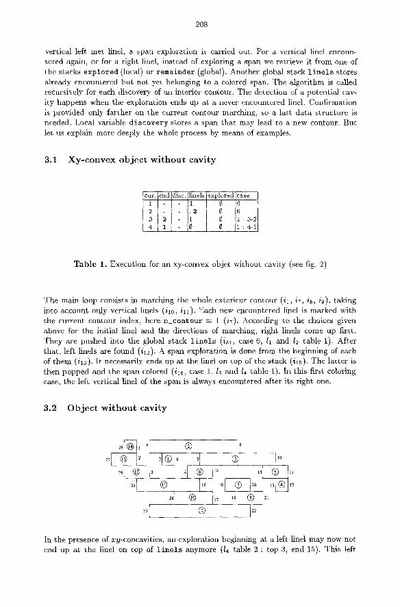
vertical left met linel, a span exploration is carried out. For a vertical linel encoun- tered again, or for a right linel, instead of exploring a span we retrieve it from one of the stacks e x p l o r e d (local) or r ema i n d e r (global). Another global stack l i n e l s stores already encountered but not yet belonging to a colored span. The algorithm is called recursively for each discovery of an interior contour. The detection of a potent ia l cav- ity happens when the exploration ends up at a never encountered linel. Confirmation is provided only farther on the current contour marching, so a last da ta s tructure is needed. Local variable d i s c o v e r y stores a span that may lead to a new contour. But let us explain more deeply the whole process by means of examples.

3 .1 X y - c o n v e x o b j e c t w i t h o u t c a v i t y

id disc. cur. e linels explored case 6 1 - " 12 ~ 6 2

3 i ~ 1:3-2 4 1:4-1

T a b l e 1. Execution for an xy-convex objet without cavity (see fig. 2)

The main loop consists in marching the whole exterieur contour (i l , i7, i~, ie), taking into account only vertical linels (i10, i11). Each new encountered linel is marked with the current contour index, here n _ c o n t o u r = 1 ( i@ According to the choices given above for the initial linel and the directions of marching, right linels come up first. They are pushed into the global stack l i n e l s (i31, case 6, 11 and 12 table 1). After that , left linels are found (i12). A span exploration is done from the beginning of each of them (it3). It necessarily ends up at the linel on top of the stack (i15). The la t ter is then popped and the span colored (i16, case 1, 18 and 14 table 1). In this first coloring case, the left vertical linel of the span is always encountered after its right one.

3 .2 O b j e c t w i t h o u t c a v i t y

27 2 O 7 ,~

25 l __ (~} 116 1 9 ~ ~

In the presence of xy-concavities, an exploration begilming at a left linel may now not end up at the linel on top of l i n e l s anymore (/4 table 2 : top 3, end 15). This left

209

linel is then pushed into l i n e l s (z20). A stack exp lored , local to the call, stores the span just explored (i26, case 3). For a right linel, we examine the exploration stored on top of exp lo red , by means of a l r e a d y exp lo red ( ) (i29, end between parentheses in the tables). If this span end do not correspond to the current linel, its beg in is simply pushed into l i n e l s (i31, case 6, li1 table 2). In the opposite case, the span is colored and the two stacks popped (i30, case 5, 19 table 2). In this second coloring case, the span left linel is always encountered before its right one.

cur . e n d disc . l inels e x p l o r e d c a s e 1 1 ~ 6 2 2 ~ 6 3 . 3 ~ 6 4 15 4-15 i . . . 4 4 -15 3 5 10 4-15 5 4-15 5-10 3 6 (10) 4-15 6 4-15 5-10 6 7 6 4-15 5 4-15 5-10 1 : 7-6 8 9 4-15 8 4-15 5-10 8-9 3 9 ( 9 ) 4-15 5 4-15 5-10 '5 : 8-9 10 (10) 4-15 . . 4 4-15 5 : 5-10 11 ( 1 5 ) 4-15 11 4-15 6

12 (15) 4-15 12 4-15 ~6 13 12 4-15 ii 4-15 i : 13-12

14 11 4-15 ..4 4-15 1 : 14-11

15 (15) .3 ~ 5 : 4-15

16 16 r 6

17 17 ~ 6

18 21 18-21 18 18-21 3 19 20 18-21 19 18-21 19-20 13 20 (20) 18-21 18 18-21 15 : 19-20 21 (21) 17 ~) 5 : 18-21 22 22 r 16 23 22 17 r 1 : 23-22

24 17 .. 16 $ Ii : 24-17

25 16 . 3 r I : 25-16 i

26 3 2 ~ 1 : 26-3

27 2 1 {~ 1 : 27-2 28 1 0 0 1 : 28-1

T a b l e 2. Execution for an objet without cavity

3.3 Object with cavities

When e x p l o r e d i s empty, a span exploration ending up at a linel different from l i n e l s top possibly means the discovery of a cavity. So this span is stored in a variable d i s c o v e r y (i21, i23, i25), local to each recursive call. Sometimes, it is a false alarm: linel d i s c o v e r y - > e n d belongs to the contour. It will be encountered later and d i s c o v e r y canceled (figure 3a, table 2). In other cases, we actually deal with a cavity (figure 3b, table 3). While d i s c o v e r y is not assigned, explored spans are pushed in global stack r ema inde r (i26, case 3, 114 table 3).

210

(a) (b)

Fig. 3. Cavities: (a) false discovery (b) true one

The assignation of d i scovery is not sufficient to detect a cavity. Three situations are possible, as illustrated on figure 4. In the first one, the end of the exploration is different from the linel on top of l i n e l s and it has mark 1 of the exterior contour. Then it is certain that a cavity lies under this last explored span or on the right of the current contour (i17, 114 table 3). In the example of figure 4a, span 2 confirms the presence under it of a cavity discovered with span 1. On figure 4d, span 8 confirms the presence on the right of the current contour of a cavity discovered with span 6.

(a) (c)

Co)

Fig. 4. Different cases for recursion

In the second situation, the current contour marching completes without any explo- ration having ended up at an exterior linel. The span d i scovery leads in this case to a cavity on the right of the current contour (is, i9, 120 et la2 table 3). In the example of figure 4b, the discovery made with span 3 is confirined only after completion of the contour marching. Finally, in the last situation, the current interior contour marching reaches d i scovery ->end. Thus it is certain that a cavity lies above the discovery span (i27). In that case, the span that actually leads to the cavity stands in explored after d iscovery . It is determined by fonction a c t u a l d e c (), that Mso transfers into remainder spans what is popped from explored. On figure 4c~ span 4 has been considered as a discovery, but the true discovery span is 5.

211

14

9

@

25 30[ �9 ]3122|| | [s4331 | I1s~TI | |

| 1 9 s |

car.

13

14

15

16

17 18

19

20

21

22

23

24

25 26

27

28

29

30

31

32

33

34

(29)1 32 I

(17) 1 8 19 20 (9)

end

24

1

6

5

32

disc l inels e x p l o r e d

13 9-20 10-27 11-26 12-25 13-24

, - ........... 13,9-20 10-27 11-26 12-25 13-24

....... 5 , 0

4

17-32 17 17-32

r e m a i n d e r

0 14-I 14-1 14-1 14-1

(32) 17-32 18 (32) 17-32 19 (32) 17-32 ........ 20 .

4 ..3

3 .2

2 i

.24

..25 26

27

19 - 28

34 29-34! i . 2 9 31 2 9 - 3 4 . 30

(31) 2 9 - 3 4 . 2 9

17-32 17-32 17-32

14-1

14-I

14-1

14-I

14-1 14-1

14-1 0 14-1 0 14-1

0 14-1 0 14-1 28-19

29-34 14-1 28-19

29-34 30-31 14-1 28-19

29-34 14-1 28-19

(34) 29-34 ........ 32 .

18 . . . . . . . . . 3 3 , - , - , . . . . . . . 34 ,

( 3 4 ) . . . . . . . . . 3 3 ,

- , . . . . . . . 3 2 ,

(32) ......... 33 ,

28

27

- h " I ..... 2o i

( 2 . 0 ) ~ I .... 27 I

29-34

0 0

1 0 - 2 7 11-26 12-25 13-24

14-1 28-19

l ~ 14-i 28-19 33-18

14-1 28-19 33-18

14-1 28-19 33-18

14-1 28-19 33-18

1 4 - 1 2 8 - 1 9 3 3 - 1 8

1 4 - 1 2 8 - 1 9

1 4 - 1

1 4 - 1

1 4 - 1

3

2

i : 15-6

I : 16-5

3

6

6

6

i :21-4

i : 22-3

1 : 23-2

6

6 6

6

3

3

3

5 : 30-31

6

3

6

1 : 29-34

6

!I : 1%32

5 : 33-18

5 : 28-19

'61 : 9-20

T a b l e 3. Execut ion for an ob je t wi th cavities

212

The detection of a cavity results in a recursive call of f i 1 l i n g () on the new interior contour (it9 et i24, case 2; 9; i28, case 4). A call to fonction s t ep_back( ) then man- ages poping l i n e l s up to d i s c o v e r y - > b e g i n included (is, in). After incrementation of the contour index, a recursion on d i s c o v e r y - > e n d takes place (in, i4, 12t et 133 ta- ble 3). Back from a recursive call, the current finel is restored to d i s c o v e r y - > b e g i n (is, c u r r e n t between parentheses in the tables, 1(29) table 3). Furthermore, after recursion (it) , and while e x p l o r e d is not empty, no span exploration happens and the fonetion a l r e a d y _ e x p l o r e d ( ) accesses to the bot tom of exp lo red , whilst d e l i s t () dequeues (i14, is0, 1(9) table 3). When e x p l o r e d gets exhausted, a l r e a

dy e x p l o r e d ( ) returns the top of remainder , whilst d e l i s t ( ) pops it 'second lls table 3).

4 Discussion

In usual methods, and following the definition from [KR89], the border is a set of pixels. Following this border poses specific problems that Pavfidis collectively termed undersampling [Pav79]. We have considered a contour as a circular list of linels. Using a "border" in the common meaning of topology, undersampling problems have been disposed of. In the general case, an exploration is saved in e x p l o r e d or remainder (i2s, i26, case 3). A span which allows to claim that d i s c o v e r y actually leads to a new cavity is saved as well (ilg, i23), except in the case when its end is an interior linel. For that kind of relatively uncommon configuration (see span 8 in figure 4d), the span will be explored twice. Most of the spans are visited only once and the redundancy of binary map ac- cesses is minor. The number of accesses to each pixel is thus in O(n). This number is in O(3n) in Pavlidis's algorithm [Pay81]. In his approach, a span exploration sys- tematically entails the one of the two neighboring spans, above and below, in order to determine the degree of this vertex in the line adjacency graph. The number of recursive calls is proportional to the number of interior points in the nai've version of the coloring algorithm. In usual "span" methods, among whom the one of Pavlidis, the size of the stack is in ratio to the number of spans in the boundary. In the proposed algorithm, the number of recursive calls is he number of cavities in the object. So the size of the stack is not a problem anyway. The fact that the method is driven by contour marching directly gives the number of cavities. The approach preserves more topological information than usual methods, the latters being driven by the waiting structure for spans. This is attractive when having 3D applications in mind.

5 Voxelized object surface traversal

Given a cut plane, surfels of a voxelized object can be divided into two sets: slice surfeis and ring surfels. The former are parallel to the cut plane and shaded in figure 5. The lat ter take their name from the fact that in each slice, they can be described by circular lists.

213

Fig . 5. Ring and slice surfels

Work is in progress to realize the sur]ace tracking of a voxelized object according to a ring/slice scheme. It can be described informaly by the following procedure:

z = initial slice;

surfel = a ring surfel in slice z;

push( surfel, z, NEG ); push( surfel, z, POS );

while ( non empty stack ) {

( surfel, z, direc ) = pop();

if ( is_( surfel, z, direc ) = pop();

ring = detect_contour( surfel ); if ( is_already_treated( ring ) ) continue;

z_next = ( direc == NEG ) ? z-I : z+l;

opp_direc = ( direc == NEG ) ? POS : NEG; if ( ring type( ring ) == EXTERNAL )

filling( ring );

else next_ring( ring );

for ( each new ring i )

if ( trailer[ i ]->z == z ) push( trailer[ i ]->surfel, z, opp_direc );

else push( trailer[ i ]->surfel, z_next, direr );

}

Fonction d e t e c t _ c o n t o u r () is a contour tracking that chains detected surfe]s as a ring. The filling algorithm is adapted for the slice surfels detection. Fonction march_ c ont our () is reduced to tracing the ring just built, whilst f i l l i n g ( ) is enriched with the man- agement of a t r a i l e r table, indexed by interior contours. Each of its elements is a trailer surfel for an incoming ring, coupled up with the corresponding slice value. The la t ter is either the current ring slice value, or the one of a contiguous slice, depending on wether the ring type (external or internal) reverses or not. The surface tracking method that is traditionnally used is the one described by Artzy et al. [AFH81]. Though elegant, the algorithm does not offer any a priori knowledge of the order in which surfels will be detected. This poses problems, especially pagination

214

when accessing the 3D binary map [FHMU85]. It seems to be worthwhile to load in memory a few contiguous slices from the voxmap (we call it a "metaslice") and to treat it without having to access it again. Furthermore, if the detection progresses slice by slice, a parallel implementation can be taken under consideration, in which each processor should work on a different metaslice. Finally, this approach is also richer in topological information. It is indeed possible to build on the fly the Reeb graph of the object [SKK91]. More generally, this ring/slice scheme may be applied to every surfels graph traversal, for example the search for local extremums on the surface. It also directly leads to a 3D filling algorithm.

6 C o n c l u s i o n

We have proposed a 2D filling Mgorithm. It is free from undersampling problems be- cause of its use of contours constituted of linels instead of pixels. The redundancy of binary map accesses is minor. The approach is recursive and the number of calls is only the number of cavities. The principle of a treatment of spans directed by contour marching directly provides the cavities. In that, it offers more topological information than usual techniques. The method finds an application in 3D voxelized objects sur- face traversal. It is in fact a basic procedure of algorithms for tracking, searching for extremum and filling of those objects surface.

The author wishes to thank the anonymous reviewers, D. Michelncci and B. P6roche for their constructive remarks on the preliminary version of this paper.

215

Appendix: pseudo-code

filling( c u r r e n t ) {

1 f o r ( e x p l o r e d = c r e a t e . s t a c k ( ) , d i s c o v e r y = n u l l , recurse = after_recursion = O, n contour = i ; ; )

{

2 if ( recurse ) {

3 step_back( discovery ); ++n_contour; 4 filling( march_contour( discovery->fin ) ); 5 current = discovery->begin; discovery = null;

6 after_recursien = I; recurse = O; }

e l s e { 7 c u r r e n t = march_contour( c u r r e n t ) ; mark( c u r r e n t ) = n_con tour ; 8 i f ( contour completed )

9 if ( discovery ) recurse = i; else return; }

}

lO if ( recurse lJ !is_vertical( current ) ]] is_colored( current ) ) 11 continue; 12 if ( is_left( surren~ ) )

{

13 if ( !after.reoursien ) end = explore.span( current );

14 else ( end = already.exploredO-~end; delistO; } 15 if ( end == top( linels ) )

{

18 color( current, end ); pop( linels ); /* i */ }

17 else if ( cavity_under.or_right( discovery, end ) ) { {

18 if ( is_exterior( end ) ) push( (current, end), remainder ); 19 recurse = I; /* 2 */

}

else( 20 push( current, linels ); 21 if ( !discovery ~ is_new( end ) )

{

22 if ( after.recursion ) {

23 enqueue( discovery = (current, end), explored ); 24 recurse = I; /* 2 */

}

25 else push( discovery = (current, end), explored ); } /* 3 */

26 else push( (current, end), discovery ? explored : remainder ); }

}

27 else if ( cavite_above( discovery, current ) ) {

28 actual_dec( discovery, explored ); recurse = I; /* 4 */ }

29 else if ( span = already_exploredO ~ span->end == current ) {

30 color( span->hegin, end ); pop( linels ); delistO; /* 5 */ }

31 else push( current, linels ); /* 6 */ }

216

R e f e r e n c e s

[AFH8t] E. Artzy, G. Frieder, and G. Herman. The theory, design, implementation and evaluation of a three-dimensional surface detection algorithm. Com- puter graphics and image processing, (15):1-24, 1981.

[CM91] J.M. Chassery and A. Montanvert. Gdomdtrie discrete en analyse d'images. Hermes, 1991.

[FHMU85] G. l~u G. Herman, C. Meyer, and 3. Udupa. Large software problems for small computers: an example from medical imaging. [EEE Software~ (2):37-47, September 1985.

[Fra95] J. Fran~on. TopologJe de khalimski-kovalevsky et algorithmique graphique. Technique et science informatiques, 14(10):1195-1219, 1995.

[FVFH90] Foley, VanDam, Feiner, and Hughes. Computer graphics: principles and practice. Addison Wesley, 2 edition, 1990.

[Heg85] G. Hegron. Synth~se d'image: algorithmes dldmentaires. AFCET Dunod, 1985.

[KR89] T. Kong and A. Rosenfeld. Digital topology: introduction and survey. Computer vision, graphics and image processing, (48):357-393, 1989.

[Lie78] H. Lieberman. How to color in a coloring book. In SIGGRAPH'78, volume 12(3), pages 111-116. ACM, August 1978.

[Mat95] G. Mathieu. Points significatifs duns un contour discret : caract~risation des cavit~s et dilatation. In 5th Discrete geometry for computer imagery, pages 249-258, 1995.

[MF82] D. Montuno and A. Fournier. Finding the x-y convex hull of a set of x-y polygons. Technical Report CSRG-148, University of Toronto, November 1982.

[Pav79] T. Pavlidis. Filling algorithms for raster graphics. Computer graphics and image processing, 10:126-141, 1979.

[Pay81] T. Pavlidis. Contour filling in raster graphics. In Proceedings SIG- GRAPH'81, volume 15(3), pages 29-36. ACM, aug 1981.

[ShaS0] U. Shani. Filling regions in binary raster images: a graph-theoretic ap- proach, in SIGGRAPH'80, volume 14, pages 321-327. ACM, 1980.

[SKK91] Y. Shinagawa. T. Kunii, and Y. Kergosien. Surface coding based on morse theory. IEEE computer graphics and applications, 11(5):66-78, September 1991.

[Smi79] A. Smith. Tint fill. In SIGGRAPH'79, volume 13(2), pages 276-283. ACM, 1979.

[TL88] G. Tang and B. Lien. Region filling with the use of the discrete green theorem. Computer vision, graphics and image processing, (42):297-305, 1988.