Smith Charts Page 1 of 27

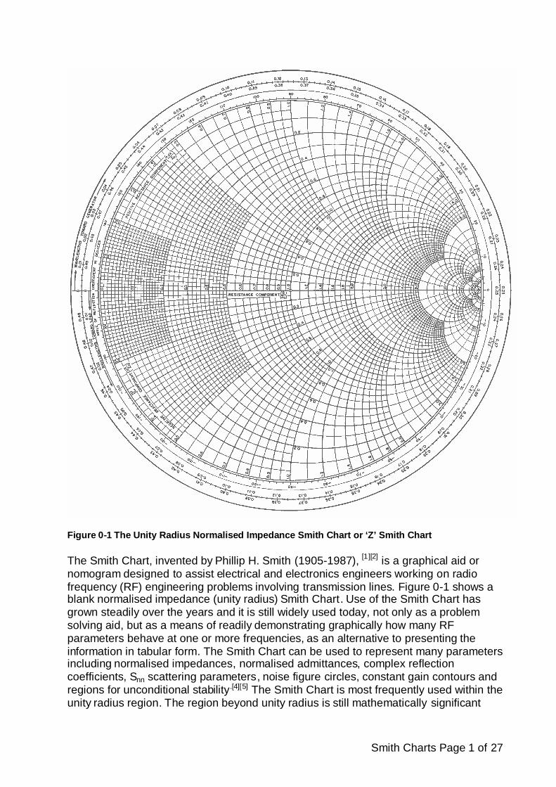
Figure 0-1 The Unity Radius Normalised Impedance Smith Chart or ‘Z’ Smith Chart

The Smith Chart, invented by Phillip H. Smith (1905-1987), [1][2] is a graphical aid ornomogram designed to assist electrical and electronics engineers working on radiofrequency (RF) engineering problems involving transmission lines. Figure 0-1 shows ablank normalised impedance (unity radius) Smith Chart. Use of the Smith Chart hasgrown steadily over the years and it is still widely used today, not only as a problemsolving aid, but as a means of readily demonstrating graphically how many RFparameters behave at one or more frequencies, as an alternative to presenting theinformation in tabular form. The Smith Chart can be used to represent many parametersincluding normalised impedances, normalised admittances, complex reflectioncoefficients, Snn scattering parameters, noise figure circles, constant gain contours andregions for unconditional stability.[4][5] The Smith Chart is most frequently used within theunity radius region. The region beyond unity radius is still mathematically significant

Smith Charts Page 2 of 27

where the magnitide of the reflection coefficient is greater than unity, such as may beencountered in, for example, negative resistance oscillator design and amplifier stabilityanalysis. [6]

Smith Charts Page 3 of 27

ContentsCONTENTS ........................................................................................................................................................ 3

FIGURES ............................................................................................................................................................ 4

TABLES .............................................................................................................................................................. 4

1 OVERVIEW............................................................................................................................................... 5

2 REAL AND NORMALISED IMPEDANCE AND ADMITTANCE......................................................... 5

3 THE NORMALISED IMPEDANCE SMITH CHART (Z SMITH CHART) .......................................... 6

3.1 THE VARIATION OF COMPLEX REFLECTION COEFFICIENT WITH POSITION ALONG THE LINE.................... 73.2 THE VARIATION OF NORMALISED IMPEDANCE WITHPOSITION ALONG THE LINE .................................... 83.3 EXAMPLE 1.........................................................................................................................................103.4 REGIONS OF THE Z SMITH CHART ........................................................................................................113.5 CIRCLES OF CONSTANT NORMALISED RESISTANCE AND CONSTANT NORMALISED REACTANCE .............12

4 THE NORMALISED ADMITTANCE SMITH CHART (Y SMITH CHART) ......................................13

4.1 EXAMPLE 2.........................................................................................................................................13

5 WORKING WITH BOTH THE Z SMITH CHART AND THE Y SMITH CHARTS ...........................15

5.1 EXAMPLE 3.........................................................................................................................................15

6 CHOICE OF SMITH CHART TYPE AND COMPONENT TYPE ........................................................16

7 USING THE SMITH CHART TO SOLVE CONJUGATE MATCHING PROBLEMS WITHDISTRIBUTED COMPONENTS......................................................................................................................17

7.1 EXAMPLE 4.........................................................................................................................................18

8 USING THE SMITH CHART TO ANALYSE LUMPED ELEMENT CIRCUITS................................21

9 USING THE SMITH CHART TO DESIGN ‘L’ MATCHING SECTIONS ...........................................23

9.1 EXAMPLE 5.........................................................................................................................................24

10 REFERENCES..........................................................................................................................................27

Smith Charts Page 4 of 27

FiguresFIGURE 0-1 THE UNITY RADIUS NORMALISED IMPEDANCE SMITH CHART OR ‘Z’SMITH CHART ............................... 1FIGURE 3-1 Z SMITH CHART CONSTRUCTION FOR EXAMPLE 1 .................................................................................11FIGURE 4-1 THE ZSMITH GRAPHICAL CONSTRUCTIONS FOR EXAMPLE 2.................................................................14FIGURE 5-1 NORMALISED IMPEDANCE SMITH CHART X AND Y EXAMPLE POINTS GIVEN INTABLE 5-1......................16FIGURE 7-1 Z SMITH CHART CONSTRUCTION FOR DISTRIBUTED LINE MATCHING PROBLEMS ..................................18FIGURE 8-1 LUMPED ELEMENT CIRCUIT USED FOR SMITH CHART ANALYSIS AT 100 MHZ SHOWN IN FIGURE 8-2.....21FIGURE 8-2 Z SMITH CHART CONSTRUCTION FOR THE LUMPED ELEMENT CIRCUIT SHOWN IN FIGURE 8-1 ...............22FIGURE 9-1 THE POSSIBLE ALTERNATIVE ‘L’ SECTION MATCHING NETWORKS .......................................................24FIGURE 9-2 SMITH CHART CONSTRUCTION FOR ‘L’ SECTION MATCHING (EXAMPLE 5)............................................26FIGURE 9-3 THE CIRCUITS RESULTING FROM EXAMPLE 5 .......................................................................................26

Tables

TABLE 4-1 REFLECTION COEFFICIENT AND NORMALISED IMPEDANCE VALUES FOR Z SMITH CHART EXAMPLE SHOWNIN FIGURE 4-1 ..............................................................................................................................................14

TABLE 5-1 Y AND Z POINTS AS PLOTTED ON THE Z SMITH CHART IN FIGURE 5-1 .....................................................15TABLE 6-1 REAL AND NORMALISED IMPEDANCES FOR THE FUNDAMENTAL CIRCUIT ELEMENTS ..............................17TABLE 6-2 REAL AND NORMALISED ADMITTANCES FOR THE FUNDAMENTAL CIRCUIT ELEMENTS............................17TABLE 8-1 SUMMARY OF TRANSFORMATIONS SHOWN IN FIGURE 8-2......................................................................23TABLE 9-1 ANALYSES OF THE SMITH CHART EXAMPLE 5 SHOWN IN FIGURE 9-2 .....................................................25

Smith Charts Page 5 of 27

1 Overview

The Smith Chart is constructed in the plane of the complex reflection coefficient andmay be scaled in normalised impedance (the most common, shown in Figure 0-1),normalised admittance or both simultaneously, using different colours to distuinguishbetween them. These are often known as the Z, Y and YZ Smith Charts respectively. [7]

Normalised scaling allows the Smith Chart to be used for problems involving anycharacteristic impedance (Z0) or system impedance, though by far the most commonlyused is 50 Ω. With simple graphical construction for a particular frequency it isstraighforward to convert between normalised impedance (or normalised admittance)and the corresponding complex voltage reflection coefficient.

The Smith Chart has circumferential scaling in wavelengths and degrees. Thewavelengths scale, used in distributed element problems, represents the distancemeasured along the transmission line between the generator and the load. The degreesscale represents the angle of the voltage reflection coefficient at the chosen point. TheSmith Chart may also be used for distributed element matching, lumped elementmatching, circuit synthesis and analysis and problems involving both distributed andlumped elements.

Use of the Smith Chart and the interpretation of the results obtained using it requires agood understanding of AC circuit theory and transmission line theory. As impedancesand admittances change with frequency, problems using the Smith Chart can only besolved manually using one frequency at a time. This is often adequate for narrow bandapplications, typically up to about 5% to 10% bandwidth, but for wider bandwidths it isusually necessary to apply Smith Chart techniques at more than one frequency acrossthe operating frequency band. Provided the frequencies are sufficiently close, theresulting Smith Chart points may be joined by straight lines to create a locus of points.

A locus of points on a Smith Chart covering a range of frequencies readily provides thefollowing information visually:

the capacitive and/or inductive behavoir of a load across the frequency range how well matched the load is at various frequencies how readily a component may be matched

If necessary, the system impedance may be altered to be more appropriate to theimpedance magnitudes being handled. For example, in dealing with bipolar transistorswhich may have input and output impedances in the order of a few Ohms, 10 Ωmay bea better choice of system impedance than 50 Ω. The accuracy of the Smith Chart isreduced for problems involving a large spread of impedances or admittances, thoughthe scaling can be magnified for individual areas to accommodate these.

2 Real and Normalised Impedance and Admittance

A transmission line with a characteristic impedance of Z0 may alternatively beconsidered to have a characteristic admittance of Y0 where

Smith Charts Page 6 of 27

00

1Z

Y

Any real impedance, ZT expressed in Ohms, may be normalised by dividing it by thecharacteristic impedance, so the normalised impedance using the lower case z, suffix Tis given by

0ZZ

z TT

Similarly, the normalised admittance (yT) may be obtained by dividing the realadmittance (YT) by the characteristic admittance, that is

0YYy T

T

The SI unit of impedance is the Ohm (Ω) and the SI unit for admittance is the Siemen(S). Normalised impedance and normalised admittance have no units. Realimpedances and real admittances must be normalised before using them on a SmithChart. The result obtained from the Smith Chart is also normalised and this must be de-normalised to obtain the real result.

3 The Normalised Impedance Smith Chart (Z Smith Chart)

Using transmission line theory, if a transmission line is terminated in an impedance ZT

which differs from its characteristic impedance, reflections will be set up and a standingwave will be formed from components of both the forward (VF) and the reflected (VR)waves. Using complex exponential notation to represent the waves:

exp( ) exp( )FV A t l

exp( ) exp( )RV B t l

where:

exp( )t is the temporal (time dependent) part of the wave and

2 f

where

is the angular frequency in radians per second (rad/s)

f is the frequency in Hertz (Hz)

t is the time in seconds (s)

Smith Charts Page 7 of 27

A and B are constants.

l is the distance measured along the transmission line from the generator in metres (m)

j is the propagation constant which does not have any units.

For this:

is the attenuation constant in Nepers per metre (Np/m)

is the phase constant in radians per metre (rad/m)

The Smith Chart is used with one frequency at a time so the temporal part of the phaseexp( )t is fixed for all equations at this frequency. All terms are actually multiplied bythis, but it is understood that it may be omitted. Therefore

exp( )FV A l

exp( )RV B l

3.1 The Variation of Complex Reflection Coefficient with Position Along theLine

The complex voltage reflection coefficient ρ(usually simply called ‘reflection coefficient’)is defined as the ratio of the reflected wave to the incident (or forward) wave. Therefore

exp( ) exp(2 )exp( )

R

F

V B l C lV A l

where C is also a constant.

For a uniform transmission line (in which γis constant) and terminated in ZT, thereflection coefficient of a standing wave varies according to the position on the line. Ifthe line is lossy (αis non-zero) this is represented on the Smith Chart by a circle ofreducing radius or spiral path. Most Smith Chart problems are greatly simplified if it issufficiently accurate to assume losses to be negligible. If this is the case, αis zero. Forthe loss free case therefore

0 j

and the expression for reflection coefficient becomes

exp(2 )C j l

where C is the magnitude of the reflection coefficient which is constant and directlyproportional to the radius of the circle drawn on the Smith Chart.

The phase constant may also be written as

Smith Charts Page 8 of 27

2

where is the wavelength within the transmission line at the test frequency. Therefore

4exp

j lC

This equation shows that, for a standing wave, the reflection coefficient and impedancerepeats every half wavelength along the line. Therefore the outer circumferential scaleof the Smith Chart, which represents distances measured along the transmission line inwavelengths, is scaled from zero to 0.50.

3.2 The Variation of Normalised Impedance with Position Along the Line

If V and I are the voltage across and the current entering the termination at the end ofthe transmission line respectively, then

F RV V V

0F RV V Z I

By dividing these equations and substituting for both the reflection coefficient

R

F

VV

and the normalised impedance of the termination (zT) given by

0T

VzZ I

gives the result:

11Tz

Alternatively, this may be expressed in terms of the reflection coefficient

11

T

T

zz

These are the equations which are used to construct the Z Smith Chart.

Both ρand zT- are expressed in complex numbers without any units. They both changewith frequency so for any particular measurement, the frequency at which it wasperformed must be stated together with the characteristic impedance.

Smith Charts Page 9 of 27

ρmay be defined in magnitude and angle on a polar diagram or Argand diagram. Anyreal reflection coefficient must have a magnitude of less than or equal to unity so, at thetest frequency, this may be expressed by a point inside a circle of unity radius. TheSmith Chart is actually superimposed on such a polar diagram. The Smith Chart scalingis designed in such a way that reflection coefficient can be converted to normalisedimpedance or vice versa. Using the Smith Chart, the normalised impedance may beobtained with appreciable accuracy by plotting the point representing the reflectioncoefficient magnitude and angle, treating the Smith Chart as a polar diagram and thenreading its value directly using the characteristic Smith Chart scaling. This technique isa graphical alternative to substituting the values in the equations. The reflectioncoefficient may beobtained from the normalised impedance using the reverseprocedure.

By substituting the expression for how reflection coefficient changes along anunmatched loss free transmission line,

exp( ) exp( )exp( ) exp( )

B l B j lA l A j l

into the equation for normalised impedance in terms of reflection coefficient

11Tz

and using Euler's identity

exp( ) cos sinj j

yields the impedance version transmission line equation for the loss free case:[8]

00

0

tan( )tan( )

LIN

L

Z jZ lZ Z

Z jZ l

where INZ is the impedance 'seen' at the input of a loss free transmission line of lengthl , terminated with an impedance LZ .

The normalised impedance version of the transmission line equation is therefore

tan( )1 tan( )

LIN

L

z j lz

jz l

The corresponding admittance versions of the transmission line equation are

00

0

tan( )tan( )

LIN

L

Y jY lY Y

Y jY l

and

Smith Charts Page 10 of 27

tan( )1 tan( )

LIN

L

y j lyjy l

The normalised impedance transmission line equation is related to the variation ofnormalised impedance around the path of a circle drawn on the Z Smith Chart with itscentre coincident with the centre of the Smith Chart. There is a similar relationship forthe normalised admittance transmission line equation and the Y Smith Chart. In bothcases the circumferential (wavelength) scaling must be used, remembering that this isthe wavelength within the transmission line and may differ from the free spacewavelength according to any dielectric that is used.

3.3 Example 1

A loss free transmission line of characteristic impedance 50 Ωis terminated with a realimpedance of 30 + j100 Ω. If the line is lengthened by 0.093 λ, what is the value of thenew termination required to ensure that the impedance seen by the generator isunchanged?

Normalising the original impedance gives the result

130 100 0.60 2.00

50z j j

The Smith Chart in Figure 3-1shows this point plotted as P1. A circle is drawn throughthis point, centred at the Smith Chart centre to represent the magnitude of the reflectioncoefficient due to the termination. The actual values of reflection coefficient and theassociated normalised impedances along the line are represented by points on thiscircle. The position in wavelengths at P1 is l1 = 0.180 λ. Moving through 0.093 λawayfrom the generator, the position of the new termination is at l2 = 0.087 λ which is marked by point P2, at which z = 0.16 + j0.60. De-normalising, the real impedance (ZP2) at pointP2 is

2 0 (0.16 0.60) 8 30PZ Z j j

Therefore the value of the new impedance required at the end of the extended line is8+j30Ω.

Converting the Z Smith Chart to a Y Smith Chart is achieved by moving the point P1through exactly 180° to the point Q1 where y =0.14 - j0.46. Moving this point through0.10 λ towards the generator moves to point Q2 where y=0.12 + j0.190. De-normalisingthis value, the real admittance at Q2 is therefore

2 0 (0.12 0.190) 0.0024 0.0038QY Y j j S

Smith Charts Page 11 of 27

Figure 3-1 Z Smith Chart construction for Example 1

3.4 Regions of the Z Smith Chart

If a polar diagram is mapped on to a cartesian coordinate system it is conventional tomeasure the angles represented by complex numbers relative to the positive x-axisusing a counter-clockwise direction for positive angles. The magnitude of a complexnumber is directly proportional to the length of a straight line drawn from the origin tothe point representing it. The Smith Chart uses the same convention for reflectioncoefficients, noting that, in the normalised impedance plane, the positive x-axis extendsfrom the center of the Smith Chart at zT = 1 ± j0 to the point zT = ∞± j∞. Inductiveimpedances have positive imaginary parts and capacitive impedances have negativeimaginary parts. Therefore the region above the x-axis represents inductiveimpedances and the region below the x-axis represents capacitive impedances.

Smith Charts Page 12 of 27

If the termination is perfectly matched, or ZT = Z0, the reflection coefficient will be zero,represented effectively by a circle of zero radius or in fact a point at the centre of theSmith Chart. If the termination was a perfect open circuit or short circuit the magnitudeof the reflection coefficient would be unity as all power would be reflected and the pointwould lie actually on the unity circumference circle.

3.5 Circles of Constant Normalised Resistance and Constant NormalisedReactance

The Z Smith Chart is composed of two families of circles: circles of constant normalisedresistance and circles of constant normalised reactance. In the complex reflectioncoefficient plane the Smith Chart itself occupies the area inside a circle of unity radiuscentred at the origin. This is identical to the circle of constant normalised resistanceequal to zero. In cartesian coordinates this circle would pass through the points (1,0)and (-1,0) on the x-axis and the points (0,1) and (0,-1) on the y-axis.

Since both ρand z are complex numbers, in general they may be expressed by thefollowing generic rectangular complex numbers where a, b, c and d are real constants:

z a jb

c jd

Substituting these into the equation relating normalised impedance and complexreflection coefficient:

11

T

T

zz

gives the following result:

2 2

2 2 2 2

1 2( 1) ( 1)a b b

c jd ja b a b

Equating coefficients of the real and imaginary parts gives

2 2

2 2

1( 1)a b

ca b

and

2 2

2( 1)

bda b

These equations describe how the complex reflection coefficients change with thenormalised impedance and may be used to construct both families of circles.[9]

Smith Charts Page 13 of 27

4 The Normalised Admittance Smith Chart (Y Smith Chart)

The Y Smith chart is constructed in a similar way to the Z Smith Chart case but byexpressing values of voltage reflection coefficient in terms of normalised admittanceinstead of normalised impedance. The normalised admittance yT is the reciprocal of thenormalised impedance zT, so

1T

T

yz

Therefore:

11Ty

and

11

T

T

yy

The Y Smith Chart scaling pattern is similar to the normalised impedance type but withthe graphic scaling only rotated through 180°.

Capacitive admittances have positive imaginary parts and inductive admittances havenegative imaginary parts. Therefore the region above the x-axis represents capacitiveadmittances and the region below the x-axis represents inductive admittances..

As with the Z Smith Chart, if the termination is perfectly matched the reflectioncoefficient will be zero, represented by a 'circle' of zero radius, actually a point at thecentre of the Smith Chart. If the termination was a perfect open or short circuit themagnitude of the voltage reflection coefficient would be unity, all power would bereflected and the point would lie on the unity circumference circle of the Smith Chart.

4.1 Example 2

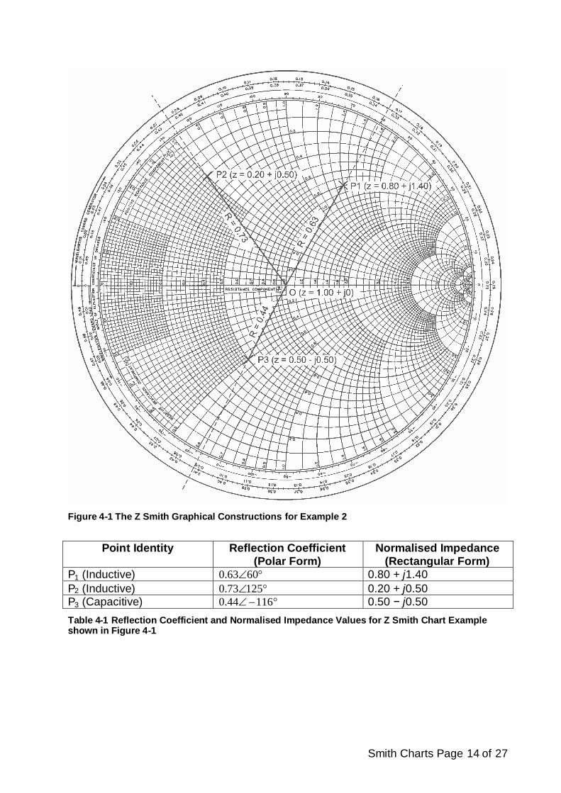
A point with a reflection coefficient magnitude 0.63 and angle 60°, represented in polarform as 0.63 60 is shown as point P1 on the Smith Chart in Figure 4-1. To plot this,one may use the circumferential (reflection coefficient) angle scale to find the 60°graduation and a ruler to draw a line passing through this and the centre of the SmithChart. The length of the line would then be scaled to P1 assuming the full Smith Chartradius to be unity. For example, if the actual radius measured from the paper was 100mm, the length OP1 would be 63 mm.

Table 4-1 gives some similar examples of points which are also plotted on the Z SmithChart in Figure 4-1. For each, the reflection coefficient is given in polar form togetherwith the corresponding normalised impedance in rectangular form. The conversion maybe read directly from the Smith Chart or obtained by substitution into the equation.

Smith Charts Page 14 of 27

Figure 4-1 The Z Smith Graphical Constructions for Example 2

Point Identity Reflection Coefficient(Polar Form)

Normalised Impedance(Rectangular Form)

P1 (Inductive) 0.63 60 0.80 + j1.40P2 (Inductive) 0.73 125 0.20 + j0.50P3 (Capacitive) 0.44 116 0.50 −j0.50

Table 4-1 Reflection Coefficient and Normalised Impedance Values for Z Smith Chart Exampleshown in Figure 4-1

Smith Charts Page 15 of 27

5 Working with Both the Z Smith Chart and the Y Smith Charts

In RF circuit and matching problems sometimes it is more convenient to work withadmittances (comprising conductances and susceptances) and sometimes it is moreconvenient to work with impedances (comprising resistances and reactances). Solvinga typical matching problem will often require several changes between both types ofSmith Chart, using normalised impedance for series elements and normalisedadmittances for parallel elements. For these a dual (normalised) impedance andadmittance Smith Chart or YZ Smith Chart may be used. Alternatively, one type may beused and the scaling converted to the other when required. In order to change from theZ Smith Chart to the Y Smith Chart or vice versa, the point representing the value ofreflection coefficient under consideration is moved through exactly 180° at the sameradius. For example, in Figure 4-1, the point P1 representing a reflection coefficient of0.63 60 has a normalised impedance of zP1 = 0.80 + j1.40. To graphically change thisto the equivalent normalised admittance point, say Q1, a line is drawn with a ruler fromP1 through the Smith Chart centre to Q1, an equal radius in the opposite direction. Thisis equivalent to moving the point through a circular path of exactly 180°. Reading thevalue from the Smith Chart for Q1, remembering that the scaling is now in normalisedadmittance, gives yP = 0.30 + j0.54. Performing the calculation

1T

T

yz

manually will confirm this.

Once a transformation from the Smith Chart Z plane to Y plane has been performed,the scaling changes to normalised admittance until such time that a later transformationback to normalised impedance is performed.

5.1 Example 3

Table 5-1 shows examples of normalised impedances and their equivalent normalisedadmittances obtained by rotation of the point through 180°at the same magnitude(radius). Again these may either be obtained by calculation or using the Smith Chartshown in Figure 5-1, converting as required between the normalised impedance andnormalised admittances planes.

Normalised Impedance Plane Normalised Admittance PlaneP1 (z = 0.80 + j1.40) Q1 (y = 0.30 −j0.54)P10 (z = 0.10 + j0.22) Q10 (y = 1.80 −j3.90)Table 5-1 y and z Points as Plotted on the Z Smith Chart in Figure 5-1

Smith Charts Page 16 of 27

Figure 5-1 Normalised Impedance Smith Chart x and y Example Points given in Table 5-1

6 Choice of Smith Chart Type and Component Type

The choice of whether to use the Z Smith Chart or the Y Smith Chart for any particularcalculation depends on which is more convenient. Impedances in series andadmittances in parallel add whilst impedances in parallel and admittances in series arerelated by a reciprocal equation. If ZTS- is the equivalent impedance of seriesimpedances and ZTP- is the equivalent impedance of parallel impedances, then

1 2 3TSZ Z Z Z

1 2 3

1 1 1 1

TPZ Z Z Z

Smith Charts Page 17 of 27

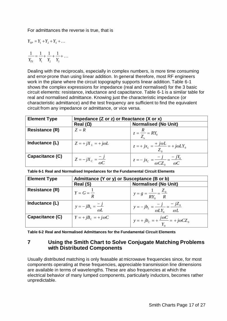
For admittances the reverse is true, that is

1 2 3TPY Y Y Y

1 2 3

1 1 1 1

TSY Y Y Y

Dealing with the reciprocals, especially in complex numbers, is more time consumingand error-prone than using linear addition. In general therefore, most RF engineerswork in the plane where the circuit topography supports linear addition. Table 6-1shows the complex expressions for impedance (real and normalised) for the 3 basiccircuit elements: resistance, inductance and capacitance. Table 6-1 is a similar table forreal and normalised admittance. Knowing just the characteristic impedance (orcharacteristic admittance) and the test frequency are sufficient to find the equivalentcircuit from any impedance or admittance, or vice versa.

Impedance (Z or z) or Reactance (X or x)Element TypeReal (Ω) Normalised (No Unit)

Resistance (R) RZ 0RY

ZR

zo

Inductance (L) LjjXZ L 0

0

LYjZ

Ljjxz L

Capacitance (C)Cj

jXZ C

CjY

CZj

jxz C 0

0

Table 6-1 Real and Normalised Impedances for the Fundamental Circuit Elements

Admittance (Y or y) or Susceptance (B or b)Element TypeReal (S) Normalised (No Unit)

Resistance (R)R

GY1

RZ

RYgy 0

0

1

Inductance (L)LjjBy L

LjZ

LYjjby L

0

0

Capacitance (C) CjjBY C 0

0

CZjY

Cjjby C

Table 6-2 Real and Normalised Admittances for the Fundamental Circuit Elements

7 Using the Smith Chart to Solve Conjugate Matching Problemswith Distributed Components

Usually distributed matching is only feasable at microwave frequencies since, for mostcomponents operating at these frequencies, appreciable transmission line dimensionsare available in terms of wavelengths. These are also frequencies at which theelectrical behavior of many lumped components, particularly inductors, becomes ratherunpredictable.

Smith Charts Page 18 of 27

For distributed components the effects on reflection coefficient, and thereforeimpedance, of moving along the transmission line must be allowed for using the outercircumferential or length scale of the Smith Chart which is calibrated in wavelengths.

7.1 Example 4

This example shows how a transmission line, terminated with an arbitrary load, may bematched at one frequency either with a series or parallel reactive component in eachcase connected at a defined position.

Figure 7-1 Z Smith Chart Construction for Distributed Line Matching Problems

Supposing a loss free air-spaced transmission line of characteristic impedance 50 Ω,operating at a frequency of 800 MHz, is terminated with a circuit comprising a 17.5 Ωresistor in series with a 6.5 nanohenry (6.5 nH) inductor. How may the line be matched?

Smith Charts Page 19 of 27

From Table 6-1, the reactance of the inductor forming part of the termination at 800MHz is

2 32.7LZ j L j fL j

so the impedance of the combination (ZT) is given by

17.5 32.7TZ j

and the normalised impedance (zT) is

0

0.35 0.65TT

Zz j

Z

This is plotted on the Z Smith Chart shown in Figure 7-1 at point P20. The line OP20 isextended through to the wavelength scale where it intersects at l1 = 0.098λ. As thetransmission line is loss free, a circle centred at the centre of the Smith Chart is drawnthrough the point P20 to represent the path of the (constant) magnitude reflectioncoefficient due to the termination. At point P21 the circle intersects with the unity circle ofconstant normalised resistance at

21 1.00 1.52Pz j

The extension of the line OP21 intersects the wavelength scale at l2 = 0.177λ, thereforethe distance from the termination to this point on the line is given by

2 1 0.177 0.098 0.079l l

Since the transmission line is air-spaced, the wavelength at 800 MHz in the line is thesame as that in free space and is given by

cf

where c is the velocity of electromagnetic radiation in free space, approximately 83 10metres per second (m/s) and f is the frequency in Hertz (Hz). The result gives λ = 375mm, making the position of the matching component 29.6 mm from the load.

The conjugate match for the impedance at P21 (zmatch) is

1.52matchz j

As the Smith Chart is still in the normalised impedance plane, from Table 6-1 a seriescapacitor Cm is required where

0 0

1.522match

m

j jz j

CZ fC Z

Smith Charts Page 20 of 27

Therefore

2.6mC pF

To match the termination at 800 MHz therefore, a series capacitor of 2.6 pF must beconnected in series with the transmission line at a distance of 29.6 mm from thetermination.

An alternative shunt match could be calculated after transforming the Z Smith Chart to aY Smith Chart. Point Q20 is the equivalent of P20 but expressed as a normalisedadmittance. Reading from the Y Smith Chart scaling, remembering that this is now anormalised admittance gives

20 0.65 1.20Qy j

In fact this value is not actually used directly. The extension of the line OQ20 through tothe wavelength scale gives l3 = 0.152λ. The earliest point at which a shunt conjugatematch could be introduced,moving towards the generator, would be at Q21, the sameposition as the previous P21, but this time representing a normalised admittance givenby

21 1.00 1.52Qy j

The distance along the transmission line is in this case

2 3 0.177 1.152 0.329l l

which, with λ = 375 mm, converts to 123 mm.

In this case the conjugate matching component is required to have a normalisedadmittance (ymatch) of

1.52matchy j

From Table 6-2 it can be seen that a negative admittance (real or normalised) wouldrequire to be an inductor, connected in parallel with the transmission line. If its value isLm, then

0

0

1.522m m

jZjj

L Y fL

This gives the result

6.5mL nH

A suitable inductive shunt match would therefore be a 6.5 nH inductor connected inparallel with the line positioned at 123 mm from the load.

Smith Charts Page 21 of 27

8 Using the Smith Chart to Analyse Lumped Element Circuits

The analysis of lumped element components assumes that the wavelength at thefrequency of operation is much greater than the dimensions of the componentsthemselves. The Smith Chart may be used to analyse such circuits in which case themovements around the chart are generated by the (normalised) impedances andadmittances of the components at the frequency of operation. In this type of analysisthe wavelength scaling on the Smith Chart circumference is not used. The circuit shownin Figure 8-1 will be analysed using a Smith Chart at an operating frequency of 100MHz. At this frequency the free space wavelength is 3 m. The component andinterconnection dimensions themselves will be in the order of millimetres so theassumption of lumped components will be valid. Despite there being no transmissionline as such, a system impedance must still be defined to enable normalisation and de-normalisation calculations. In theory this could be any value but Z0 = 50Ωif at allpossible is strongly recommended since this value is so widely adopted in testequipment and data sheets. If the impedances involved at the operating frequency differvery substantially from 50 Ω, it might be helpful to define a value of Z0 closer to thosevalues to avoid dealing with points close to the Smith Chart circumference. For exampleZ0 = 10 Ωmight be a better choice for bipolar transistors which tend to haveimpedances of just a few Ohms. The circuit in Figure 8-1 has a 50 Ωresistor so Z0 willbe taken as 50 Ωin this case.

Figure 8-1 Lumped Element Circuit Used for Smith Chart Analysis at 100 MHz shown in Figure 8-2

Smith Charts Page 22 of 27

Figure 8-2 Z Smith Chart Construction for the Lumped Element Circuit Shown in Figure 8-1

The Smith Chart shown in Figure 8-2 is used for the analysis of the circuit shown inFigure 8-1. Points with suffix P are in the Z plane and points with suffix Q are in the Yplane. The analysis starts with a Z Smith Chart looking into R1 only, with no othercomponents present. As R1 = 50 Ωis the same as the system impedance, themagnitude of the reflection coefficient at this point is zero represented by a point at thecentre of the Smith Chart. The first transformation is OP1 is along the line of constantnormalised resistance which, in this case, is the addition of a normalised impedance of -j0.80. From Table 6-1, this is equivalent to a series capacitor of 40 pF. TransformationsP1 to Q1 and P3 to Q3 are from the Z Smith Chart to the Y Smith Chart andtransformation Q2 to P2 is the reverse. Table 8-1 shows all transformations with theassociated formulas, the final of which brings the reflection coefficient magnitude backto zero at the centre of the Smith Chart and a perfect 50 Ωmatch. The network wouldtherefore be closely matched to 50 Ωat 100 MHz.

Smith Charts Page 23 of 27

Trans-formation

Plane x or yNormalisedValue

C or L Formula to Solve Result

O→P1 Z -j0.80 C(Series)

1

0

01

80.0CjY

ZCjj

C1 = 40 pF

Q1→Q2 Y -j1.49 L (Shunt)

1

0

01

49.1LjZ

YLjj

L1 = 53 nH

P2→P3 Z -j0.23 C(Series)

2

0

02

23.0CjY

ZCj

j

C2 = 138 pF

Q3→O Y +j1.14 C (Shunt)03

0

314.1 YCjY

Cjj

C3 = 36 pF

Table 8-1 Summary of Transformations Shown in Figure 8-2

9 Using the Smith Chart to Design ‘L’ Matching Sections

A simple and very versatile means of matching one impedance to another can beachieved by using an ‘L’ section circuit comprising either of the configurations ofcapacitors and/or inductors shown in Figure 9-1. [10] With good quality (high Q factor)components typically suitable up to a few hundred megahertz the loss of the matchingnetwork should be minimal. In each case the match will be effective over a relativelysmall bandwidth.

Provided that the impedance magnitudes being matched do not differ too greatly theresult of the matching network design using Smith Charts should define realistic valuesof capacitance and inductance. In general it is easier to match using capacitors as theyare more readily available than inductors, cheaper and their performance is morepredictable over frequency. Capacitors also generally have higher Q-factors and havemore stable values over frequency.

Any impedance may be matched to another at one frequency using at least 2 of thematching networks shown in Figure 9-1. This is demonstrated with the followingexample.

Smith Charts Page 24 of 27

Figure 9-1 The Possible Alternative ‘L’ Section Matching Networks

9.1 Example 5

Show how an impedance of 10 +j10Ωmay be matched to 50 Ωwith 2 different ‘L’section matching networks at an operating frequency of 500 MHz.

Using a system impedance (Z0) of 50 Ω, if ZT is the real termination, then

10 10TZ j

The positive reactive part implies an inductance L where

Smith Charts Page 25 of 27

10 2j j L j fL

which gives

3.2L nH

and the normalised impedance zT is given by

0

0.2 0.2TT

Zz jZ

This is represented by the point P1 plotted on the Z Smith Chart shown in Figure 9-2.

An additional circle has been added to Figure 9-2 which maps precisely to the unityconstant normalised conductance (or unity constant normalised resistance) circle in thealternate Smith Chart plane. In the absence of a YZ Smith Chart, this is a usefulreference as any point on this cirlcle will map directly to the corresponding circle in theother plane when undergoing a Z to Y or Y to Z Smith Chart transformation. Any pointon either of these circles can be conjugately matched with just one reactive component.

Starting with the Z Smith Chart, P1 may be mapped to O via either of the followingroutes:

P1 to P2 (arc); P2 to Q1 (Z to Y) and Q1 to O (arc) P1 to P3 (arc); P3 to Q2 (Z to Y) and Q2 to O (arc)

The analyses of both cases are shown in Table 9-1, using the formulas given in Table6-1 and Table 6-2.

Trans-formation

Plane x or yNormalisedValue

C or L Formula to Solve Result

P1→P2 Z +j0.21 L(Series)

0 0

20.21 j L j fLjZ Z

L1 = 3.3 nH

Q1→O Y +j1.95 C(Shunt) 0

0

1.95 2j C

j j fCZY

C1 = 12.4 pF

P1→P3 Z -j0.61 C(Series)

0 0

0.612

j jjCZ fCZ C2 = 10.4 pF

Q2→O Y -j1.95 L(Shunt)

0

0

1.952

jZjj

LY fL

L2 = 8.2 nH

Table 9-1 Analyses of the Smith Chart Example 5 Shown in Figure 9-2

Smith Charts Page 26 of 27

Figure 9-2 Smith Chart Construction for ‘L’ Section Matching (Example 5)

The two alternative matching circuits derived from the results shown in Table 9-1 areshown in Figure 9-3.

Figure 9-3 The Circuits Resulting from Example 5

Smith Charts Page 27 of 27

10 References

1. Smith, P. H.; Transmission Line Calculator; Electronics, Vol. 12, No. 1, pp 29-31,January 1931

2. Smith, P. H.; An Improved Transmission Line Calculator; Electronics, Vol. 17, No. 1,p 130, January 1931

3. Ramo, Whinnery and Van Duzer (1965); "Fields and Waves in CommunicationsElectronics"; John Wiley & Sons; pp 35-39. ISBN

4. Pozar, David M. (2005); Microwave Engineering, Third Edition (Intl. Ed.); John Wiley& Sons, Inc.; pp 64-71. ISBN 0-471-44878-8.

5. Gonzalez, Guillermo (1997); Microwave Transistor Amplifiers Analysis and Design,Second Edition; Prentice Hall NJ; pp 93-103. ISBN 0-13-254335-4.

6. Gonzalez, Guillermo (1997) (op. cit);pp 98-1017. Gonzalez, Guillermo (1997) (op. cit);p 978. Hayt, William H Jr.; "Engineering Electromagnetics" Fourth Ed;McGraw-Hill

International Book Company; pp 428 433. IBSN 0-07-027395-2.9. Davidson, C. W.;"Transmission Lines for Communications with CAD

rograms";Macmillan; pp 80-85. ISBN 0-333-47398-110.Gonzalez, Guillermo (1997) (op. cit);pp 112-125