Electrical Engineering (2018) 100:2319–2328https://doi.org/10.1007/s00202-018-0707-7

ORIG INAL PAPER

Field–circuit model of the radial active magnetic bearing system

Bronisław Tomczuk1 · Dawid Wajnert1

Received: 13 December 2017 / Accepted: 6 July 2018 / Published online: 12 July 2018© The Author(s) 2018

AbstractPaper presents a mathematical model of the radial active magnetic bearing, which is indented for the simulation of themagnetic bearing dynamic response. The circuit model of the bearing is based on differential equations. The circuit modelhas incorporated results of magnetic field analysis, which led to the creation of the field–circuit model. Presented model ofthe magnetic bearing takes into account the necessary control system. The experimental results are presented to validate theproposed model.

Keywords Radial active magnetic bearing · An electromagnetic actuator · Finite element method · Magnetic field analysis ·The control system

1 Introduction

Magnetic bearings (MBs) represent an alternative support ofthe rotor in comparison with traditional bearings, i.e., ball orjournal ones.MBs have found applications inmany industrialdevices, for example, in high-speed turbines, energy storageflywheels, turbomolecular pumps, turbogenerators, machinetool spindles and compressors [1–3]. The benefits of usingmagnetic bearings are well known [1]. Owing to the con-tactless operation of the rotor, the bearing provides a lackof friction, absence of lubricating substance, good vibrationdamping, online monitoring of the operation and reducedmaintenance and operation costs.

Magnetic suspension dedicated to electric machine usu-ally consists of two radial and one axial electromagnetic actu-ators and a control system. The actuator of the radial activemagnetic bearing (RAMB) comprises two elements—a sta-tor and rotor. The interaction between the stator and rotoris based on the principle of the electromagnetic interaction.The current flowing in the windings causes the pull of themovable ferromagnetic material. Unfortunately, the stablelevitation of the RAMB rotor is only achievable by usingposition controllers.

B Dawid Wajnertd.wajnert@po.opole.pl

1 Department of Electrical Engineering and Mechatronics,Opole University of Technology, ul. Prószkowska 76,45-758 Opole, Poland

In this paper, a field–circuit model of the RAMB sys-tem dedicated to the simulation of the transient states isdescribed. The model is based on a set of the differentialequations implemented inMATLAB/Simulink software. Themain parameters of the RAMBwere obtained from the mag-netic field analysis. The model also includes the necessarycontrol systemwith PID controllers for the rotor position andPI controllers for currents excited in windings. The presentedsimulation model was compared with the real object.

The aim of this paper is to present an effective and fastmodel of theRAMBsystem,which can be used to test variouscontrollers as well as determine its parameters.

2 Structure of the active magnetic bearing

The construction of the RAMB actuator consists of a statorand rotor. In order to significantly reduce the eddy currentseffects, the stator and rotor were fabricated from 0.5-mm-thick silicon steelM600-50A.The cross sectionof theRAMBactuator is presented in Fig. 1. The winding of the stator haswound twelve coils, which allows creating several configura-tions of the magnetic field excitation. It is possible to obtainthree sections, four sections and six sections of the winding.In this paper, we consider four sections of thewinding, whichpermits to implement the differential driving mode [1]. Forsuch mode, currents excited in windings are equal to:

123

2320 Electrical Engineering (2018) 100:2319–2328

Fig. 1 The cross section of the RAMB actuator

Table 1 The main parameters of the RAMB actuator

Parameter Value

The outer diameter of the stator 53 mm

Length of the stator 45 mm

Width of the air gap 1 mm

The turn number of one winding 114

Bias current 5 A

Maximal current 10 A

I1 � Ib + icy, (1.a)

I2 � Ib + icy, (1.b)

I3 � Ib − icy, (1.c)

I4 � Ib − icx , (1.d)

where Ib denotes the bias current and icy and icx indicatethe control currents for y- and x-axis, respectively. The biascurrent is used for linearization of the magnetic force char-acteristic within the operating range of the magnetic bearing[1].

The main parameters of the RAMB actuator are presentedin Table 1.

3 Mathematical model of the activemagnetic bearing

Magnetic field distribution was obtained from the 2D finiteelement method (FEM). The field analysis is based on thecalculation of the magnetic vector potential �A [4]. Although

Fig. 2 The geometry of 2D FEM model and a quarter of the mesh

the 2D FEM model neglects the end effects of the magneticfield, they have a minor impact on integral parameters ofthe magnetic field [5]. In numerical model, the eddy currentseffects were neglected and the magnetic field was consideredto be stationary. However, the impact of the manufacturingprocess was taken into account in the model, which changesthe magnetic properties of narrow layers of the stator androtor sheets [6, 7]. Hence, the air gap in the simulation modelwas increased in comparison with the real object.

The calculation area includes the whole geometry of theRAMB actuator cross section. Dirichlet’s boundary condi-tions were assumed at its edges (Fig. 2).

The finite element mesh was carefully selected, in orderto obtain the balance between accurate results and short timeof computation. The stator and rotor subregions were dis-cretized with the fine mesh. The discretization of the airgap has a significant impact on the force calculation results.Therefore, the air gap was divided into two subregions.

Based on the FEM algorithm, two cases of the magneticfield distribution in the RAMB actuator were calculated. Inthe first case, the central position of the rotor and the biascurrent Ib excitation in windings were assumed. For suchassumption, the magnetic forces Fx and Fy are equal tozero (Fig. 3). Magnetic field density in each electromagnet isapproximately 0.74 T. That value constitutes half of the max-imal field density (Bmax �1.5 T) assumed for the RAMB.

In the second case, the central position of the rotor, thecontrol current icy equal to 5 A was assumed. Thus, the cur-rent excited in the first winding is equal to 10 A, whereas inthe third winding it is equal to zero. In this case, the magneticforce Fy in the y direction is equal to 68.9 N. This value rep-

123

Electrical Engineering (2018) 100:2319–2328 2321

Fig. 3 Magnetic field distribution for central position of the rotor andthe bias current excitation

Fig. 4 Magnetic field distribution for central position of the rotor andthe control current icy �5 A

resents the maximal magnetic force of the RAMB actuator.Magnetic field density in the first electromagnet is equal to1.42 T (Fig. 4).

The calculated magnetic flux distribution was used to esti-mate themagnetic force generated by all four electromagnets.The magnetic force was calculated fromMaxwell stress ten-sor. The calculations were executed for various cases, overthe entire operating range of the magnetic bearing currentsI1, I2, I3, I4 ∈ (0, 10 A) and the various positions of the rotorshaft x, y ∈ (−400, 400 µm).

The calculated values of the magnetic force generated bythe first electromagnet, as a function of thewinding current I1and the shaft position y, are given in Fig. 5. The flux linkagewas calculated from the following equation [8]:

Ψ �N∑

k�1

φk �N∑

k�1

¨

S

�B · d�s, (2)

Fig. 5 The magnetic force F1 in function of the current I1 and positiony of the rotor

Fig. 6 The flux linkage Ψ1 in function of the current I1 and position yof the rotor

where N is the turn number of the stator winding and φk isthe magnetic flux linking with one turn of the winding.

The flux linkage of the first electromagnet as a functionof the winding current I1 and the shaft position y is given inFig. 6.

The magnetic flux linked with the windings was usedfor calculating the dynamic inductances and the velocity-induced voltage coefficient [9]. The dynamic inductance Ld1was calculated from the following expression:

Ld1(y, I1) � ∂Ψ1(y, I1)

∂ I1, (3)

123

2322 Electrical Engineering (2018) 100:2319–2328

Fig. 7 The dynamic inductance Ld1 in function of the rotor position yand the current I1

whereas the velocity-induced voltage coefficient hv1 was cal-culated from the expression:

hv1(y, I1) � ∂Ψ1(y, I1)

∂y, (4)

Figure 7 presents values of the dynamic inductance Ld1 infunction of the rotor position and the current intensity. It isnoticeable that the value of the dynamic inductance increaseswith increasing the coordinate y. This effect is due to decreas-ing value of the air gap. The exception is the range of highvalues of the current intensity and high values of the rotordeflectionwhen the values of the dynamic inductance slightlydecrease. The reason of that is saturation of the magneticmaterial.

Figure 8 presents the velocity-induced voltage coefficientin function of the rotor position and the current I1. The valueof the velocity-induced voltage coefficient increases in accor-dance with the current value and position of the rotor in they-axis. Also, there is a region, where the value of the velocity-induced voltage coefficient is decreasing. The reason for thisis the saturation of the magnetic material, because of theproximity of the stator and rotor.

The main parameters of MBs are current ki and positionks stiffness [10]. These parameters are often included in theequations of motion. The parameters are calculated from thefollowing expressions:

kiy � ∂Fy(icy, y)

∂icy

∣∣∣∣y�const

(5.a)

Fig. 8 The velocity-induced voltage coefficient in function of the rotorposition y and current I1

Fig. 9 Current stiffness kiy in function of the rotor position y and controlcurrent icy

ksy � ∂Fy(icy, y)

∂y

∣∣∣∣icy�const

(5.b)

Figures 9 and 10 present the current kiy and position stiff-ness ksy of considered MB for bias current Ib �5 A infunction of the rotor position y and the control current icy.

123

Electrical Engineering (2018) 100:2319–2328 2323

Fig. 10 Position stiffness ksy in function of the rotor position y andcontrol current icy

The mathematical model of the RAMB actuator isdescribed by a set of the ordinary differential equations:

u1 � R1i1 + Ld1(i1, y)di1dt

+ hv1(i1, y)dy

dt(6.a)

u2 � R2i2 + Ld2(i2, x)di2dt

+ hv2(i2, x)dx

dt(6.b)

u3 � R3i3 + Ld3(i3, y)di3dt

+ hv3(i3, y)dy

dt(6.c)

u4 � R4i4 + Ld4(i4, x)di4dt

+ hv4(i4, x)dx

dt(6.d)

md2y

dt2� F1(i1, y) − F3(i3, y)

+ meSω2 cos(2πωt) −

√2

2mg (7.a)

md2x

dt2� F2(i2, x) − F4(i4, x)

+ meSω2 sin(2πωt) −

√2

2mg (7.b)

The voltage and current balance Eqs. (6.a, 6.b, 6.c) gov-ern the electrical characteristics of the RAMB actuator. TheparameterRi (where, i�1, 2, 3, 4) denotes the winding resis-tance. Parameters Ldi and hvi (where, i �1, 2, 3, 4) indicatethe dynamic inductance of thewindings andvelocity-inducedvoltage coefficients, respectively. Equations (7.a, 7.b) gov-ern the rotor motion and include the magnetic forces, Fi

(where, i �1, 2, 3, 4) generated by four electromagnets.Also, these equations incorporate static unbalance of the rotorwith the eccentricity eS, which denotes a difference betweenthe rotor center and the center of the rotor mass. Symbols

Table 2 Value of the constant parameters for the mathematical model

Parameter Value

Windings resistance, R1, R2, R3, R4 1.4 �

Mass, m 2.6 kg

Eccentricity, eS 40 µm

m and ω indicate the mass and the angular velocity of therotor, respectively. The equations of the motion include thegravity force acting on the rotor, which is equally dividedbetween both axes. Equations (6.a, 6.b, 6.c) and (7.a, 7.b)were implemented in Simulink/MATLAB software. The val-ues of constant parameters of the mathematical model arelisted in Table 2. The winding resistances and mass of therotor were measured and constitute input data. The value ofthe eccentricity eS was assumed in order to achieve a similar,to the physical object, dynamic response of the rotor duringrotation.

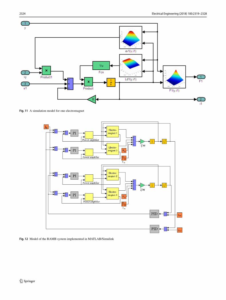
The other parameters, like dynamic inductances, velocity-induced voltage coefficients and magnetic forces are nonlin-ear functions of the currents excited in windings and positionof the rotor. Therefore, these parameters were obtained frompreviously presented finite element model and were incorpo-rated in the model as lookup tables. Figure 11 presents thesimulation model of the first electromagnet that correspondsto Eq. (6.a).

The RAMB is an inherently unstable device that meanswithout the control system stable levitation of the rotor isimpossible. Therefore, in order to obtain dynamic responses,the control system for considered MB was designed. It con-sists of four switching power amplifiers, four PI currentcontrollers and two PID controllers of the rotor position.Figure 12 presented the layout of the RAMB mathematicalmodel with the control system.

The pole placement method was used to obtain values ofparameters for the current and position controllers [11].

The coefficients values for the position controllers PIDare given in Table 3, whereas the coefficients for the currentcontrollers PI are given in Table 4.

4 Simulation results

Figure 13a, b presents time responses of the currents i1 andi3 excited in electromagnets and position of the rotor in y-axis for the rotor lifting. The counterpart waveforms, in thex-axis, are similar.

The value of the control current, for both axes in a steadystate, is equal to 1.3 A. For this state, the electromagnetsgenerate only the forces to balance the weight of the rotor.The settling time ts of the MB system equals 36.8 ms.

123

2324 Electrical Engineering (2018) 100:2319–2328

Fig. 11 A simulation model for one electromagnet

Fig. 12 Model of the RAMB system implemented in MATLAB/Simulink

123

Electrical Engineering (2018) 100:2319–2328 2325

Table 3 Value of the coefficients for the position controllers

KP (A/m) K I (A s/m) KD (A/m s)

17,417.4 839,446.9 74.8

Table 4 Value of the coefficients for the current controllers

KP (A−1) K I (s/A)

0.1006 66.84

Fig. 13 Time responses of electromagnets currents (a) and the rotordisplacement in the y-axis (b) for the rotor lifting

Figure 14a, b presents simulation results for the rotor rota-tion. The rotor deviation, caused by the static unbalance, isequal to 69.7 µm.

Fig. 14 Simulation results for the rotor rotation with the speed of6000 rpm: a the currentwave in electromagnets 1 and 3,b rotor displace-ment—the solid line indicates the position of the rotor during rotation,the dotted line indicates mechanical constrain of the rotor movement

5 Experimental verificationof the simulations

Figure 15 shows plots of the normal, to the stator surface,magnetic flux density component, which was calculated andmeasured in the middle of the RAMB stator depth. Due tothe small air gap, the magnetic flux density values were mea-sured without the rotor presence. The sensor of magnetic fluxdensity was slid according to angle α and was 1 mm awayfrom the iron surface of the pole teeth.

123

2326 Electrical Engineering (2018) 100:2319–2328

Fig. 15 The normal component of the magnetic flux density inside thestator of the RAMB actuator excited by the current intensity of Ib �5 A

One can find a good agreement between magnetic fluxdensity values obtained from the field simulation and frommeasurements. Differences between the calculated and mea-sured results do not exceed a few percents.

For the central position of the rotor, themagnetic force val-ues, in function of the control currents icx and icy, are nearlylinear, which are presented in Figs. 16 and 17.However, a dif-ference between the calculated and measured values of themagnetic force is noticeable. The largest differences occurfor the maximal control current values, and they are equal to5.0% for x-axis and 8.8% for the y-axis.

In Fig. 18, an outline of the test stand which contains theRAMB system is presented. The RAMB actuator is suppliedby the switching power amplifier with supplying voltageUdc

�35 V and the switching frequency f PWM of the PWM sys-tem equal to 20 kHz. All control tasks are carried out by themagnetic bearing controller (MBC), which was based on theARM7 microcontroller. An additional motor supplied withthe variable frequency drive was employed for the rotationof the RAMB rotor. An analog input card was used for mea-suring of all signals. Figure 19 presents a photograph of thetest stand.

Figure 20a, b presents time responses ofmeasured currentsexcited in electromagnets and the rotor displacement in x-and y-axis for the rotor lifting.

The values of control currents icy, icx in a steady state areapproximately equal to 1.5 A, and they are slightly higher forthe real object in comparison with those obtained from thecomputer simulation. This difference could be the result of

Fig. 16 Characteristic of the control current icx in function of externalforce F in the x-axis

Fig. 17 Characteristic of the control current icy in function of externalforce F in the y-axis

omitting the eddy currents in the finite element model. Theeddy currents are responsible for decreasing the values of thecurrent and position stiffness. The settling time of the MBsystem is equal to 28.8 ms and its value is lower than in thecomputer simulation.

In Fig. 21, measurement results during the rotor rotationare presented. The maximal deviation of the rotor is equal to

123

Electrical Engineering (2018) 100:2319–2328 2327

Fig. 18 Test stand for the measurement verification of the simulated transients in the RAMB operation

Fig. 19 A photograph of the test stand. (1) A variable frequency drive,(2) an electric motor, (3) the radial magnetic bearing, (4) switchingpower amplifier andmagnetic bearing controller and (5) a measurementcard

73.9 µm. In contrast to the simulation, the rotor center pathis not a circle which may indicate an asymmetry of the forcegeneration.

Table 5 consists of gathered values of the RAMB systemperformance indicators. The parameters tSx and tSy denotethe rotor settling time for the rotor lifting, respectively, in xand y direction. Parameters J1x and J1y denote the integralof the square error e(t) calculated during rotor lifting:

J1x �tk∫

0

[ex (t)]2dt (8.a)

J1y �tk∫

0

[ey(t)

]2dt, (8.b)

where tk denotes the final time of the system response obser-vation.

Parameter J2 denotes maximal deviation of the rotor cen-ter.

One can notice that the settling time and the integral ofthe square error took higher values for the simulation modelthan for the real object. It could be due to the higher value ofdamping in the physical model than in the numerical simu-lation.

Fig. 20 Time responses of electromagnets currents (a) and the rotordisplacement in x- and y-axis (b) for the rotor lifting

123

2328 Electrical Engineering (2018) 100:2319–2328

Fig. 21 Measurement results for the rotor rotationwith speed 6000 rpm:a the current wave in electromagnets 1 and 3, b rotor displacement—thesolid line indicates the position of the rotor during rotation, the dottedline indicates mechanical constrain of the rotor movement

Table 5 Values of the transient performance indicators

Transientperformanceindicator

Measurement Calculation

tSx (ms) 29.1 36.8

tSy (ms) 28.5 36.8

J1x (mm2 s) 4.1·10−4 5.1·10−4

J1y (mm2 s) 4.3·10−4 5.1·10−4

J2 (µm) 73.9 69.7

6 Conclusion

In the paper, the field–circuit model of the active magneticbearing system including its control system was presented.The correctness of the presented dynamic model was con-firmed by measurements of the selected parameters underoperating condition. They were calculated, for the lifting ofthe shaft as well as for the rotor rotation with the speed of6000 rpm.

Open Access This article is distributed under the terms of the CreativeCommons Attribution 4.0 International License (http://creativecommons.org/licenses/by/4.0/), which permits unrestricted use, distribution,and reproduction in any medium, provided you give appropriate creditto the original author(s) and the source, provide a link to the CreativeCommons license, and indicate if changes were made.

References

1. Schweitzer G,Maslen H (2009)Magnetic bearings, theory, design,and application to rotating machinery. Springer, Berlin

2. Canders W-R, May H, Palka R (1998) Topology and performanceof superconducting magnetic bearings. COMPEL Int J ComputMath Electr Electron Eng 17:628–634. https://doi.org/10.1108/03321649810220946

3. Budig PK (2010) Magnetic bearings and some new applications.In: XIX international conference on electrical machines—ICEM2010, Rome

4. Meeker D (2015) FEMM 4.2, user manual5. Wajnert D (2014) Comparison of magnetic field parameters

obtained from 2D and 3D finite element analysis for an active mag-netic bearing. Solid State Phenom 214:130–137

6. Antila M, Lantto E, Arkkio A (1998) Determination of forces andlinearized parameters of radial active magnetic bearings by finiteelement technique. IEEE Trans Magn 34:684–694

7. Polajzer B, Stumberger G, Ritonja J, Dolinar D (2008) Variationsof active magnetic bearings linearized model parameters analyzedby finite element computation. IEEE Trans Magn 44:1534–1537

8. Tomczuk B, Koteras D,Waindok A (2015) The influence of the legcutting on the core losses in the amorphous modular transformers.COMPEL Int J Comput Math Electr Electron Eng 34:840–850

9. TomczukB, SchröderG,WaindokA (2007) Finite element analysisof the magnetic field and electromechanical parameters calculationfor a slotted permanent magnet tubular linear motor. IEEE TransMagn 43:3229–3236

10. Gosiewski Z, Mystkowski A (2008) Robust control of active mag-netic suspension: analytical and experimental results. Mech SystSignal Process 22:1297–1303

11. Franklin G (2002) Feedback control of dynamic systems. PrinceHall, Newark

Publisher’s Note Springer Nature remains neutral with regard to juris-dictional claims in published maps and institutional affiliations.

123