Fibonacci Heaps

CS 252: Algorithms

Geetika Tewari 252a-al

Smith College

December, 2000

My Contribution

- Understanding Fibonacci Heaps. This involved understanding:

- Operations of Creation, Union, Insert, Extract-Min, Delete, Decrease Key

- The circular linked list data structure used for the heap

- Reading about Amortized analysis, the Potential Function and Binomial heaps

- The proof which gives the name Fibonacci to these heaps

- Understanding an application of Fibonacci Heaps in the Shortest Paths problem

- Researching Leda implementations of Fibonacci Heaps or other data structures that use these heaps

- Implementing Dijkstra’s Shortest Path algorithm in Leda using different priority queues, one of which is the Fibonacci Heap

-Experimenting, Recording and Comparing the running times of Dijkstra using 6 different LEDA priority queues that use 6 different heaps

Research Tools and Resources UsedBooks Consulted:

- Algorithms, by Cormen, Leiserson, and Rivest, page 420-439. All examples taken from there.

-Data Structures, Algorithms and Program Style, by James F. Korsh, page 247-248 provide a good explanation of the proof by Induction on how Fibonacci Heaps get their name

Websites Consulted:

-Complete Web Tutorial on Fibonacci Heaps http://wwwcsif.cs.ucdavis.edu/~fletcher/classes/110/lecture_notes/lec17.html

-Example of the implementation of a LEDA Priority Queue

http://www.cs.umbc.edu/~zwa/Algorithms/CMSC641.html

-Online Tutorial and Animation of Fibonacci Heaps

http://www-cse.uta.edu/~holder/courses/cse5311/lectures/l13/node13.html

Programming Tools

-LEDA Online User Manual

http://www.cs.bgu.ac.il/~cgproj/LEDA/Index.html

Programs and Excel Files created that are submitted for project

1. The main program used to run all tests is

dpq.cpp

2. The compilation line used to compile it is in the file

dpq_compile

3. A typescript is included to show how the program runs and expects user interaction.

252a-al_typescript

4. A bash shell file runs all the dpq.cpp tests many times so that average time can be collected:

rundijtests*

5. An input data file is also provided called

data_dij

Outline1. Introduction: What is a Fibonacci Heap?

- Why Fibonacci Heap, proof of D(n), some definitions

2. Fibonacci Heap operations, with step by step focus on

• Insertion

• Extract-Minimum Node

• Decrease-Key

3. Comparison of Running Times with other Heaps

4. Application to Shortest Path Problem

5. Experiments:

• LEDA Dijkstra Performance using different priority queues based on different heaps

• Graphical Results

• Comparison of running times

6. Concluding Remarks

What is a Fibonacci Heap?

data structure… advantages of removal & concatenation

23 7 3

38 52 30 18

39 41

17

35

46 26

24

Min [H]

- Heap ordered Trees

- Rooted, but unordered

- Children of a node are linked together in a Circular, doubly linked List, E.g node 52

child list of node 52

root list of Fibonacci HeapMinimu

m node

Node Pointers

- left [x]

- right [x]

- degree [x] - number of children in the child list of x

- - mark [x]

Properties of Binomial Heaps relevant for the understanding of Fibonacci Heaps

Quick Summary

1. 2k nodes

2. k = height of tree

3. (ki) nodes at depth i

4. Unordered binomial tree Uk has root with degree k greater than any other node.

Children are trees U0, U1, .., Uk-1 in some order.

What is a Fibonacci Heap?….. (cont.)

• Collection of unordered Binomial Trees.

•Support Mergeable heap operations such as Insert, Minimum, Extract Min, and Union in constant time O(1)

• Desirable when the number of Extract Min and Delete operations are small relative to the number of other operations.

• Most asymptotically fastest algorithms for computing minimum spanning trees and finding single source shortest paths, make use of the Fibonacci heaps.

Why is it called a Fibonacci Heap? 0 1 1 2 3 5 8 ….

1. Lemma:

If x has degree K in a Fibonacci heap, then size(x) (nodes rooted at x and x itself) is at least F(K+2), meaning the Fibonacci number of index k+2.

Proof:

Let sk be the maximum possible value of size(z) over all nodes z such that

degree[z] = k. So s0=1, s1=2, s3=3.Let y1, y2,…yk be the children of x in the

order in which they were linked to x.

To compute the lower bound on size(x), we count one for x itself and one for

the first child y1 (for which size(y1)>=1) and then apply the Lemma for the other children:-

Use this Lemma:

”Let x be any node in a Fibonacci heap, and suppose that degree[x]=k. Let y1,y2,…,yk

be the children of x in the order in which they were linked to x, from the

earliest to the latest. Then, degree[y1]>=0 and degree[y i]>=i-2 for i=2,3,…,k.”

Proof continued

We thus have

Size(x) >= sk

>= 2 + Sum of(si - 2) from i=2….k

We can now show by induction on k that sk >= Fk+2 for all nonnegative integers k.

For the Inductive step we assume, k>=2 and si>=Fi+2, for i=0,1, ….,k-1.

We have

Sk >= 2 + Sum of (si – 2) from i=2…k

>= 2 + Sum of (Fi) from i=2…k

>= 1 + Sum of (Fi) from i=0…Fi

= Fk+2 follows from the Lemma described on previous slide

Hence, Size(x) >= sk >= Fk+2

Hence the name Fibonacci Heap arises.

2. Corollary: For n-node Fibonacci Heap, D(n) (the maximum degree of a node) is largest if all nodes are in one tree. Recall Binomial tree properties:

The maximum degree is at depth=1, (k1) = k nodes at depth 1 for tree

with 2k nodes.

If n = 2k, then k = lg n

D(n) <= k = lg n

D(n) = O(lg n)

An Upper bound on D(n), the maximum degree of a node, in an n-node Fibonacci Heap

Amortized analysis ……. a quick definition

The complexity analysis of Fibonacci Heaps is heavily dependent upon the “potential method” of amortized analysis

- The time required to perform a sequence of data structure operations is averaged over all the operations performed.

- Can be used to show that average cost of an operation is small, if you average over a sequence of operations, even though a single operation might be expensive

Fibonacci Heap Operations

1. Make Fibonacci Heap - Assign N[H] = 0, min[H] = nil

Amortized cost is O(1) 2. Find Min - Access Min[H] in O(1) time

3. Uniting 2 Fibonacci Heaps

- Concatenate the root lists of Heap1 and Heap2

- Set the minimum node of the new Heap

- Free the 2 heap objects

- Note: No consolidation of trees occurs!

Amortized cost is equal to actual cost of O(1)

Insert – amortized cost is O(1)- Initialize the structural fields of node x, add it to the root list of H- Update the pointer to the minimum node of H, min[H]- Increment the total number of nodes in the Heap, n[H]

23 7 3

38 52 30 18

39 41

17

35

46 26

24

Min [H] Example

23 21 3

38 52 30 18

39 41

17

35

46 26

24

Min [H]

7

Insert (continued)Notice- Node 21 has been inserted- Red Nodes are marked nodes – they will become relevant only in the delete operation

- Note: No consolidation of trees occurs!

Example

Extract Minimum Node – amortized cost is O(D(n))- make a root out of each of the minimum node’s children- remove the minimum node from the root list, min ptr to right(x)- Consolidate the root list by linking roots of equal degree and key[x] <= key[y], until every root in the root list has a distinct degree value. (uses auxiliary array)

23 7 3

38 52 30 18

39 41

17

35

46 26

24

Min [H]

23 21 38 52

30

18

39 41

17

35

46 26

24

Min [H]

7

23 21 38 52

30

18

39 41

17

35

46 26

24 7

0 1 2 3 4

w,x

A

23 21 38 52

30

18

39 41

17

35

46 26

24 7

0 1 2 3 4

x,w

A

23 21 38 52

30

18

39 41

17

35

46 26

24 7

0 1 2 3 4

w,x

A

23

21 38 52

30

18

39 41

17

35

46 26

24 7

0 1 2 3 4

X

W

A

23

21 38 52

30

18

39 41 17

35

46 26

24 7

0 1 2 3 4

X

W

23

21 38 52

30

18

39 41 17

35

46 26

24

7

0 1 2 3 4

X

W

Auxiliary Array

Here is a step by step Example

A

23

21 38 52

30

18

39 41 17

35

46 26

24

7

0 1 2 3 4

w,x

Extract Minimum Node (Example continued)- Root Nodes are stored in the auxiliary array in the index corresponding to their degree- Hence node 7 is stored in index 3 and node 21 is stored in index 0

Extract Minimum Node (continued)

Notice- The pointer min[H] is updated to the new minimum

A

23

21 38 52

30

18

39 41 17

35

46 26

24

7

0 1 2 3 4

w,x

Extract Minimum Node (Example continued)- Further, node 18 is stored in index 1- There are no root nodes of index 2, so that array entry remains empty- Now the algorithm iterates through the auxiliary array and links roots of equal degree such that key[x] <= key[y],

A

23 21

38

52 30

18

39 41 17

35

46 26

24

7

0 1 2 3 4

w,x

Extract Minimum Node (Example continued)- Nodes 21 and 52 are linked so that node 21 has degree 1, and it is then linked to node 18

Extract Minimum Node (Example continued) - The pointers of the auxiliary array are updated - But there are now no more remaining root nodes of duplicate degrees

A

23 21

38

52 30

18

39 41 17

35

46 26

24

7

0 1 2 3 4

w,x

23 21

38

52 30

18

39 41 17

35

46 26

24

7

min [H]

Extract Minimum Node (Example continued)- Extract-Min is now done - The pointer min[H] is finally updated to the new minimum

A node is marked if:

- At some point it was a root

- then it was linked to anther node

- and 1 child of it has been cut

- Newly created nodes are always unmarked

- A node becomes unmarked when ever it becomes the child of another node.

We mark the fields to obtain the desired time bounds. This relates to the “potential function” used to analyze the time complexity of Fibonacci Heaps.

Understanding marked nodes (red in previous slides) essential for understanding Fibonacci Heap Decrease Key Operation

Decrease-Key - amortized cost is O(1)

- Check that new key is not greater than current key, then assign new key to x

- If x is a root or if heap property is maintained, no structural changes - Else -Cut x: make x a root, remove link from parent y, clear marked field of x -Perform a Cascading cut on x’s parent y(relevant if parent is marked): - if unmarked: mark y, return - if marked: Cut y, recurse on node y’s parent

- if y is a root, returnThe Cascading cut procedure recurses its way up the tree until a root, or an unmarked node is found

- Update min[H] if necessary

23 21

38

52 30

18

39 41 17

35

46 26

24

7

min [H]

Decrease-Key - amortized cost is O(1)- We start with a heap- Suppose we want to decrease the keys of node 46 to 15

Here is a step by step Example

23 21

38

52 30

18

39 41 17

35

15

26

24

7

min [H]

Decrease-Key (example continued)- Since the new key of node 46 is 15 it violates the min-heap property, so it is cut and put on the root- Suppose now we want to decrease the key of node 35 to 5

23 21

38

52 30

18

39 41 17

5 15

26

24

7

min [H]

Decrease-Key (example continued)- So node 5 is cut and place on the root list because again the heap property is violated- But the parent of node 35, which is node 26, is marked, so we have to perform a cascading cut

23 21

38

52 30

18

39 41 17

5 15 26

24

7

min [H]

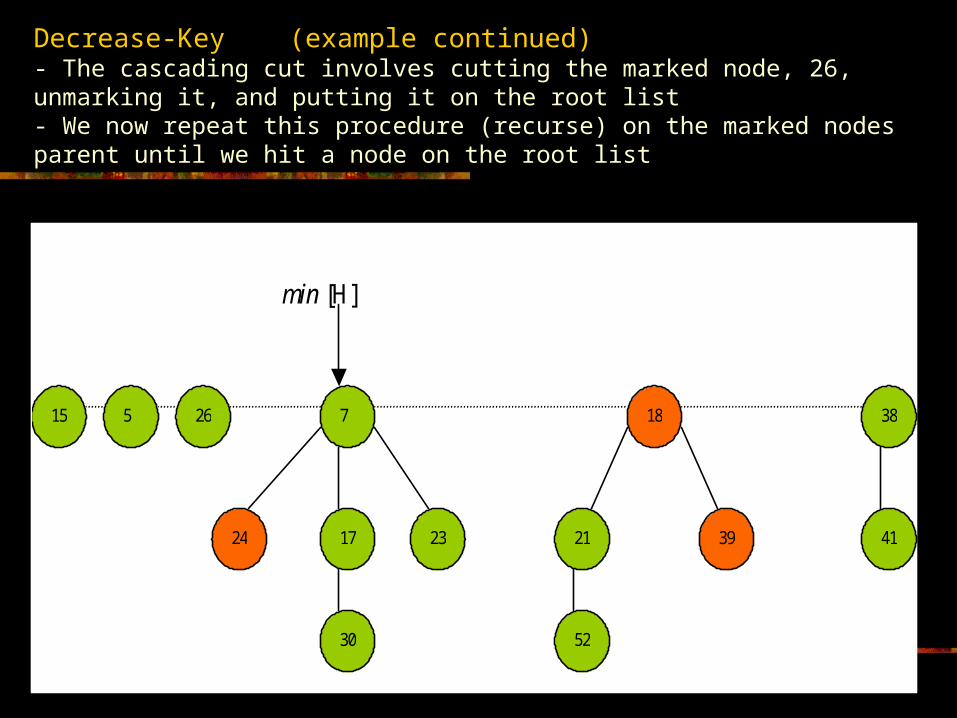
Decrease-Key (example continued)- The cascading cut involves cutting the marked node, 26, unmarking it, and putting it on the root list- We now repeat this procedure (recurse) on the marked nodes parent until we hit a node on the root list

23 21

38

52 30

18

39 41 17

5 15 26 24 7

min [H]

Decrease-Key (example continued)- Since the next node encountered in the cascading cut procedure is a root node – node 7 – the procedure terminates- Now the min heap pointer is updated

Delete-Key - amortized cost is O(D(n))

- Call Decease-Key on the node x that needs to be deleted in H, assigning negative infinity to it

- Call Extract-Min on H

Now that we have gone through the operations of the Fibonacci Heaps, we can do a comparison of the time taken for these operations with other heaps

      

      

Procedure Binary Heap

(worst case)

Binomial Heap

(worst case)

Fibonacci Heap

Make-Heap θ(1) θ(1) θ(1)

Insert θ(lgn) O(lgn) θ(1)

Minimum θ(1) O(lgn) θ(1)

Union θ(n) O(lgn) θ(1)

Decrease-Key θ(lgn) θ(lgn) θ(1)

Extract-Min θ(lgn) θ(lgn) O(lgn)

Delete θ(lgn) θ(lgn) O(lgn)

(Amortized)

For dense graphs which have many edges, the O(1) amortized call of Decrease-Key adds up to a big improvement over the θ(lgn) worst case time of Binomial or Binary Heaps.

Applications to Shortest Path Problem

Recall single-source/all nodes shortest path problem : Find shortest path from node s in graph to every other node, given non-negative weights on edges

This algorithm runs in O(N^2) time if the storage set for nodes is maintained as a linear array. For instance, each ExtractMin operation takes O(N) time and there are N such operations.

• Selecting next shortest distance is Extract-Min on heap

• Updating distance estimates is Decrease-Key on heap

• Total Extract mins: O(N log(N))

• Update edges: O(E) since each of the | E | Decrease-Key operations takes O(1) amortized time

Total cost: O(N logN + E)

which is good if number of edges is smaller than N2, graph is sparse.

Instead, implement the priority queue as a Fibonacci heap!

Experiments using LEDA

- LEDA does not provide the Fibonacci Heap data structure in its libraries, so a Fibonacci Heap LEDA object cannot be instantiated.

- Priority Queue Implementations based on different types of heap structures are available. The default implementation uses a Fibonacci Heap.

-The LEDA PQ object provide a good basis for testing and analyzing the complexity of some well known algorithms, such as …..

Dijkstra’s Shortest

Path Algorithm

Implementation Plan - Graph density - Time function - Accuracy

-Create program dpq.cpp that Implements the LEDA provided dijkstra() function with type of Priority Queue as a function argument

-Program reads input by LEDA’s read_int() function:

- n Nodes

- m Edges

- max Maximum Cost Edge

- Type of Priority Queue that Dijkstra will use (1-6 where 1 is Fibonacci Heap)

-Run the program on graphs of density 1000-128000 (n) nodes and 3n edges(multiples of 2)

- Write a bash file to run tests overnight

-Record the program running times using Leda’s used_time() function. Repeat 10 times to get an average running times

-Plot the running times against the graph density for each Priority Queue

-Use Logarithmic Scale to better visualize the results

Results and Analysis

Table Displaying the average time complexity of Dijkstra on random graphs of different density using 6 different LEDA Priority Queue Implementations.

Average Densitiy of the Graph: Number of Vertices and EdgesNodes (n) 1000 2000 4000 8000 16000 32000 64000 128000Edges (3n) 3000 6000 12000 24000 48000 96000 192000 384000Fibonacci Heap 0.01 0.04 0.07 0.18 0.34 0.89 2.11 4.89k-Heap 0.01 0.03 0.07 0.13 0.36 0.71 1.65 3.84m-Heap 0.01 0.02 0.04 0.10 0.21 0.40 1.03 2.56list-pq 0.02 0.03 0.11 0.61 2.77 11.34 45.68 334.12p-heap 0.01 0.03 0.05 0.10 0.27 0.63 1.48 2.98r-heap 0.01 0.02 0.04 0.14 0.24 0.49 1.24 2.75bin-heap 0.01 0.02 0.04 0.11 0.21 0.61 1.30 3.03

Graph of Results Running Times of Dijkstra's Algorithm with Different Priority Queue Implementations

0.00

50.00

100.00

150.00

200.00

250.00

300.00

350.00

400.00

1000 2000 4000 8000 16000 32000 64000 128000

Graph Density (Number of Nones (n), Edges (3n) )

Ave

rage

Run

ning

Tim

e (s

econ

ds)

Fibonacci Heap List Priority Queue K-ary Heap Monotone Heaps Pairing Heaps Redistributive Heaps Binary Heaps

List PQ dominates! delete_min

and find_min

O(n)

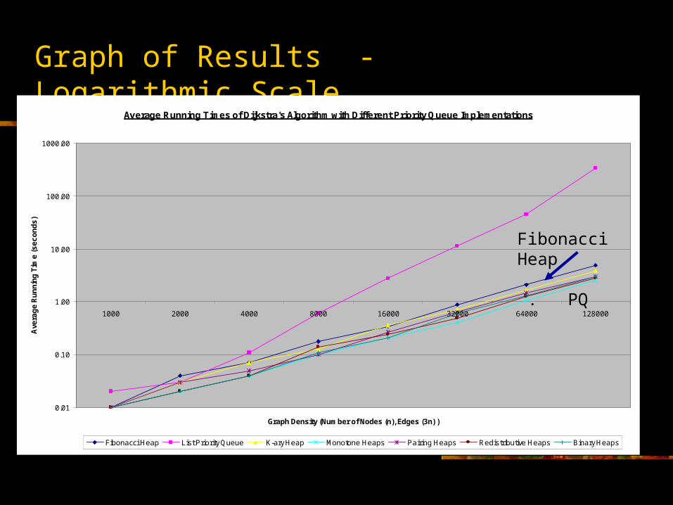
Graph of Results - Logarithmic Scale

Average Running Times of Dijkstra's Algorithm with Different Priority Queue Implementations

0.01

0.10

1.00

10.00

100.00

1000.00

1000 2000 4000 8000 16000 32000 64000 128000

Graph Density (Number of Nodes (n), Edges (3n) )

Ave

rag

e R

un

nin

g T

ime

(s

ec

on

ds

)

Fibonacci Heap List Priority Queue K-ary Heap Monotone Heaps Pairing Heaps Redistributive Heaps Binary Heaps

Fibonacci Heap . PQ

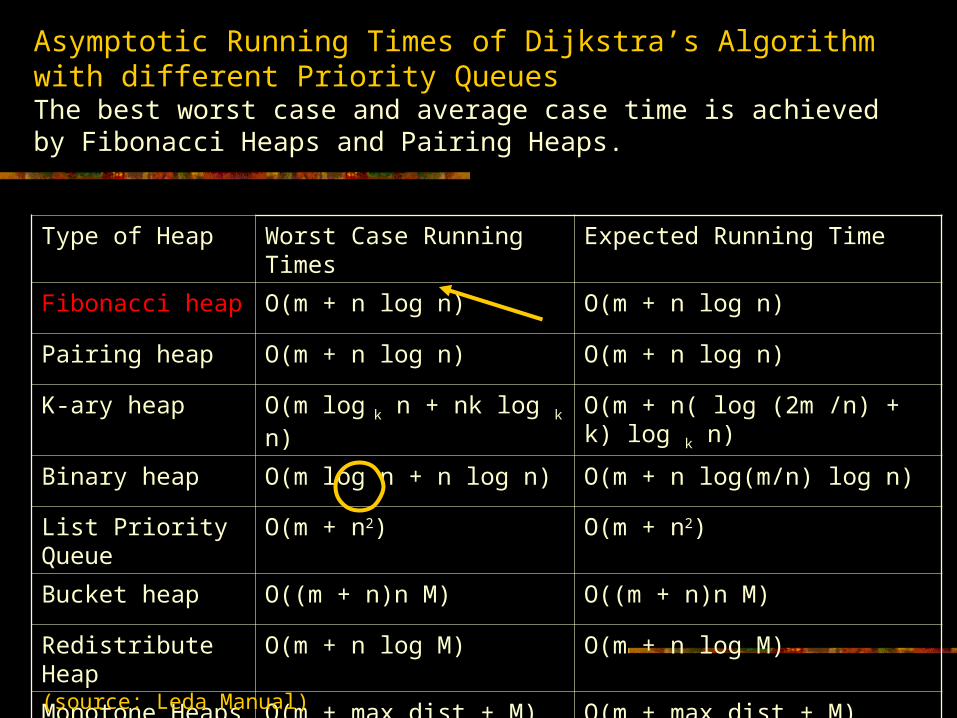
Asymptotic Running Times of Dijkstra’s Algorithm with different Priority Queues The best worst case and average case time is achieved by Fibonacci Heaps and Pairing Heaps.

Type of Heap Worst Case Running Times Expected Running Time

Fibonacci heap O(m + n log n) O(m + n log n)

Pairing heap O(m + n log n) O(m + n log n)

K-ary heap O(m log k n + nk log k n) O(m + n( log (2m /n) + k) log k n)

Binary heap O(m log n + n log n) O(m + n log(m/n) log n)

List Priority Queue O(m + n2) O(m + n2)

Bucket heap O((m + n)n M) O((m + n)n M)

Redistribute Heap O(m + n log M) O(m + n log M)

Monotone Heaps O(m + max_dist + M) O(m + max_dist + M)

(source: Leda Manual)

Concluding Remarks

- Fibonacci Heaps are mostly of theoretical interest, but are quite tedious to implement. If a much simpler data structure with the same amortized time bounds as Fibonacci Heaps were developed, it would be of great practical use as well.

- However, some source code is available, so borrow………….

http://www.boost.org/libs/pri_queue/f_heap.html