
FERMILAB-PUB-17-082-AD ACCEPTED First Principles...
10
0018-9499 (c) 2016 IEEE. Personal use is permitted, but republication/redistribution requires IEEE permission. See http://www.ieee.org/publications_standards/publications/rights/index.html for more information. This article has been accepted for publication in a future issue of this journal, but has not been fully edited. Content may change prior to final publication. Citation information: DOI 10.1109/TNS.2016.2644663, IEEE Transactions on Nuclear Science 1 First Principles Modeling of RFQ Cooling System and Resonant Frequency Responses for Fermilab’s PIP-II Injector Test J. P. Edelen, Member, IEEE, A. L. Edelen, Student Member, IEEE, D. Bowring, Member, IEEE, B. E. Chase, J. Steimel, S. G. Biedron, Senior Member, IEEE, S. V. Milton, Fellow, IEEE Abstract—In this paper we develop an a priori method for simulating dynamic resonant frequency and temperature re- sponses in a radio frequency quadrupole (RFQ) and its associated water-based cooling system respectively. Our model provides a computationally efficient means to evaluate the transient response of the RFQ over a large range of system parameters. The model was constructed prior to the delivery of the PIP-II Injector Test RFQ and was used to aid in the design of the water-based cooling system, data acquisition system, and resonance control system. Now that the model has been validated with experimental data, it can confidently be used to aid in the design of future RFQ resonance controllers and their associated water-based cooling systems. Without any empirical fitting, it has demonstrated the ability to predict absolute temperature and frequency changes to 11% accuracy on average, and relative changes to 7% accuracy. I. I NTRODUCTION In ion accelerators, radio frequency quadrupoles (RFQs) are used to provide both acceleration and strong focusing of the beam, typically for injection into subsequent acceleration stages. In order to ensure proper acceleration and focusing in the RFQ, low-level RF (LLRF) control is used to maintain the field amplitude and phase. In the presence of detuning this is accomplished in part by increasing the forward power, thus taking advantage of the available power overhead in the RF amplifiers. However, the cost of additional power overhead scales with the power of the amplifier. At the power requirements for most RFQs, it is more cost effective to design and implement RF and water systems that facilitate precise control of the RFQ’s resonant frequency. A model that fully characterizes the dynamic resonant frequency response of the RFQ under various operating conditions including system- level details facilitates the specification of both the water cooling system and the resonant frequency controller, thus reducing design risk and enabling better system optimization. Simulation of thermal effects in RFQs are often conducted using multi-physics codes such as ANSYS [1, 2, 3 ,4]. These simulations treat the RFQ as a stand-alone system. While this is highly valuable, it is generally too difficult to study both the RFQ thermal response and the full cooling system response in a simulation tool with this level of detail. A simplified thermal J. P. Edelen ([email protected]), D. Bowring, B. E. Chase, and J. Steimel are with the Fermi National Accelerator Laboratory, Batavia IL, 60510, USA A. L. Edelen, S. G. Biedron, and S. V. Milton are with Colorado State University, Fort Collins CO, 80523, USA capacitance model has been used previously to study system- level effects in RF electron guns [5, 6, 7]. This technique is well suited for cavities with a single water-temperature-to- resonant-frequency relationship; however, RFQs have a water- temperature-to-resonant-frequency relationship that depends on both the vane and the wall temperatures. The RFQ for the PIP-II Injector Test is currently being commissioned at Fermilab in support of a proposed upgrade to the accelerator complex. This upgrade will increase proton intensity for the next generation of neutrino experiments [8, 9, 10]. In order to understand the frequency transients for our RFQ on a detailed level and over long time scales, we have developed a model that encompasses the temperature and frequency response of the RFQ in conjunction with the thermal response of the cooling system. The thermal response model of the RFQ was an extension of the classical lumped thermal capacitance technique [5, 6, 7]. The temperature-to-frequency coefficients used in this model for the vanes and walls were determined from a set of detailed multi-physics simulations of the RFQ without the dynamics of the external cooling system. These were conducted at LBNL [11]. In this paper we begin with an overview of the water cooling system used for this RFQ, followed by a discussion of our modeling technique. We discuss the model’s ability to capture complex thermal relationships in the RFQ. We then demonstrate the performance of the model by comparing temperature and frequency predictions to measured data from the RFQ and water system. These comparisons were done both at low average power (pulsed operation) and at high average power (CW operation), thus demonstrating that this modeling technique can be used to characterize a RFQ water cooling system for both low-power applications and high- power applications. II. OVERVIEW OF THE RFQ AND WATER SYSTEM The RFQ is 4.45 meters long, and is composed of four separate modules connected along the longitudinal axis. It is designed to operate at 162.5 MHz with a nominal RF input power of 100 kW CW. Chilled water is supplied to the RFQ by two parallel loops: one for the inner (vane) channels and one for the outer (wall) channels, as illustrated in Figure 1. The channels are fed via an external cooling circuit, supplied with temperature-regulated water. The ratio of cold water to warm FERMILAB-PUB-17-082-AD ACCEPTED Operated by Fermi Research Alliance, LLC under Contract No. DE-AC02-07CH11359 with the United States Department of Energy
Transcript of FERMILAB-PUB-17-082-AD ACCEPTED First Principles...
0018-9499 (c) 2016 IEEE. Personal use is permitted, but republication/redistribution requires IEEE permission. See http://www.ieee.org/publications_standards/publications/rights/index.html for more information.
This article has been accepted for publication in a future issue of this journal, but has not been fully edited. Content may change prior to final publication. Citation information: DOI 10.1109/TNS.2016.2644663, IEEETransactions on Nuclear Science
1
First Principles Modeling of RFQ Cooling Systemand Resonant Frequency Responses for Fermilab’s
PIP-II Injector TestJ. P. Edelen, Member, IEEE, A. L. Edelen, Student
Member, IEEE, D. Bowring, Member, IEEE, B. E. Chase, J. Steimel, S. G. Biedron, SeniorMember, IEEE, S. V. Milton, Fellow, IEEE
Abstract—In this paper we develop an a priori method forsimulating dynamic resonant frequency and temperature re-sponses in a radio frequency quadrupole (RFQ) and its associatedwater-based cooling system respectively. Our model provides acomputationally efficient means to evaluate the transient responseof the RFQ over a large range of system parameters. The modelwas constructed prior to the delivery of the PIP-II Injector TestRFQ and was used to aid in the design of the water-based coolingsystem, data acquisition system, and resonance control system.Now that the model has been validated with experimental data,it can confidently be used to aid in the design of future RFQresonance controllers and their associated water-based coolingsystems. Without any empirical fitting, it has demonstrated theability to predict absolute temperature and frequency changes to11% accuracy on average, and relative changes to 7% accuracy.
I. INTRODUCTION
In ion accelerators, radio frequency quadrupoles (RFQs)are used to provide both acceleration and strong focusing ofthe beam, typically for injection into subsequent accelerationstages. In order to ensure proper acceleration and focusing inthe RFQ, low-level RF (LLRF) control is used to maintainthe field amplitude and phase. In the presence of detuningthis is accomplished in part by increasing the forward power,thus taking advantage of the available power overhead inthe RF amplifiers. However, the cost of additional poweroverhead scales with the power of the amplifier. At the powerrequirements for most RFQs, it is more cost effective to designand implement RF and water systems that facilitate precisecontrol of the RFQ’s resonant frequency. A model that fullycharacterizes the dynamic resonant frequency response of theRFQ under various operating conditions including system-level details facilitates the specification of both the watercooling system and the resonant frequency controller, thusreducing design risk and enabling better system optimization.
Simulation of thermal effects in RFQs are often conductedusing multi-physics codes such as ANSYS [1, 2, 3 ,4]. Thesesimulations treat the RFQ as a stand-alone system. While thisis highly valuable, it is generally too difficult to study both theRFQ thermal response and the full cooling system response ina simulation tool with this level of detail. A simplified thermal
J. P. Edelen ([email protected]), D. Bowring, B. E. Chase, and J. Steimelare with the Fermi National Accelerator Laboratory, Batavia IL, 60510, USA
A. L. Edelen, S. G. Biedron, and S. V. Milton are with Colorado StateUniversity, Fort Collins CO, 80523, USA
capacitance model has been used previously to study system-level effects in RF electron guns [5, 6, 7]. This techniqueis well suited for cavities with a single water-temperature-to-resonant-frequency relationship; however, RFQs have a water-temperature-to-resonant-frequency relationship that dependson both the vane and the wall temperatures.
The RFQ for the PIP-II Injector Test is currently beingcommissioned at Fermilab in support of a proposed upgradeto the accelerator complex. This upgrade will increase protonintensity for the next generation of neutrino experiments [8,9, 10]. In order to understand the frequency transients forour RFQ on a detailed level and over long time scales, wehave developed a model that encompasses the temperature andfrequency response of the RFQ in conjunction with the thermalresponse of the cooling system. The thermal response modelof the RFQ was an extension of the classical lumped thermalcapacitance technique [5, 6, 7]. The temperature-to-frequencycoefficients used in this model for the vanes and walls weredetermined from a set of detailed multi-physics simulations ofthe RFQ without the dynamics of the external cooling system.These were conducted at LBNL [11].
In this paper we begin with an overview of the watercooling system used for this RFQ, followed by a discussionof our modeling technique. We discuss the model’s abilityto capture complex thermal relationships in the RFQ. Wethen demonstrate the performance of the model by comparingtemperature and frequency predictions to measured data fromthe RFQ and water system. These comparisons were doneboth at low average power (pulsed operation) and at highaverage power (CW operation), thus demonstrating that thismodeling technique can be used to characterize a RFQ watercooling system for both low-power applications and high-power applications.
II. OVERVIEW OF THE RFQ AND WATER SYSTEM
The RFQ is 4.45 meters long, and is composed of fourseparate modules connected along the longitudinal axis. It isdesigned to operate at 162.5 MHz with a nominal RF inputpower of 100 kW CW. Chilled water is supplied to the RFQ bytwo parallel loops: one for the inner (vane) channels and onefor the outer (wall) channels, as illustrated in Figure 1. Thechannels are fed via an external cooling circuit, supplied withtemperature-regulated water. The ratio of cold water to warm
FERMILAB-PUB-17-082-AD ACCEPTED
Operated by Fermi Research Alliance, LLC under Contract No. DE-AC02-07CH11359 with the United States Department of Energy

0018-9499 (c) 2016 IEEE. Personal use is permitted, but republication/redistribution requires IEEE permission. See http://www.ieee.org/publications_standards/publications/rights/index.html for more information.
This article has been accepted for publication in a future issue of this journal, but has not been fully edited. Content may change prior to final publication. Citation information: DOI 10.1109/TNS.2016.2644663, IEEETransactions on Nuclear Science
2
water will later be used to regulate the resonant frequencyof the RFQ. Each module of the RFQ has its own waterdistribution manifold.
Fig. 1: Cross-section of RFQ showing locations of the vaneand wall cooling channels
The external cooling circuit itself consists of water distribu-tion, two pumps that maintain a constant flow of water into theRFQ, two flow control valves that regulate how much chilledwater is mixed into each sub-circuit, and an intermediate skidthat regulates the average chilled water supply temperature.The intermediate skid has its own independent temperaturecontrol system that maintains the output temperature to within±0.28◦C (±0.5◦F). Figure 2 shows a schematic overview ofthe cooling system. For illustration purposes, we have lumpedtogether the different modules of the RFQ and displayed thewater distribution manifolds as a single supply (after VT3and WT3) and return (before VT2 and WT2) to the RFQ.It is important to note that the system is subject to transportdelays for the return water and for the supply water due tothe pump and supply lines being located outside the cave.The helical mixers are located just before the distributionmanifold to minimize the transport delay between the watermixing point and the RFQ. There are six locations where wehave high-resolution temperature sensors suitable for the usein the resonance control system. These sensors are located atthe chilled water supply point (WT1 and VT1 for the wallsand vanes respectively), on the return line (WT2 and VT2for the walls and vanes respectively), and after the mixingpoints (WT3 and VT3 for the walls and vanes respectively).Additionally we have flow and pressure meters throughout thecooling system with high resolution flow meters on the chilledwater supply lines.
III. OVERVIEW OF THE MODELING TECHNIQUE
In order to construct a model that is simple enough forlong-timescale simulations (on the order of the characteristicresponse of the RFQ, 30-40 minutes), but also producesaccurate results, we approximate the thermal dynamics in
Fig. 2: Block diagram of the water cooling system
the RFQ, the fluid dynamics of the cooling system, and thegeometry of the entire system.
For the cooling system, we begin by approximating each ofthe water distribution manifolds as two supply and return pipes(i.e. one set for the vane circuit and one set for the wall circuit).This simplifies the transport model and heat transfer model ofthe cooling system. Additionally, we assume that the transportdelays in the plumbing manifold are small compared with thelong transport delays associated with the distribution system.We also assume that pumps on the cooling skids completelyand perfectly compensate for changes in the chilled supplyflow, as designed. In reality, this compensation is not perfect.Finally, we assume that the helical mixers are performing idealmixing between the chilled water and the return water. Forthe RFQ, the geometry of the walls and vanes were simplifiedinto two individual thermal capacitances, with a coupling termbetween them to account for the heat transfer between thewalls and vanes. This ignores localized effects on individualsections of the vanes and walls but should capture enoughdetail to predict temperature and resonant frequency shiftsof the RFQ and cooling system with reasonable accuracy.Estimates of the parameters in this model are described inSection IV.
A. Thermal response of the RFQ
The thermal model of the RFQ begins with the classicallumped capacitance [5] for an RF cavity
Tout(t) =Tinitial +1
C
∫ t
0
Prf(t)dt
− 1
C
∫ t
0
((Tout(t) − Tin(t))V
A
)dt.
(1)
0018-9499 (c) 2016 IEEE. Personal use is permitted, but republication/redistribution requires IEEE permission. See http://www.ieee.org/publications_standards/publications/rights/index.html for more information.
This article has been accepted for publication in a future issue of this journal, but has not been fully edited. Content may change prior to final publication. Citation information: DOI 10.1109/TNS.2016.2644663, IEEETransactions on Nuclear Science
3
Here, Tout(t) is the temperature of the water leaving the cavity.We assume that the temperature of the water leaving the cavityis approximately equal to the temperature of the cavity [ibid].C is the thermal capacitance [J/◦C] of the cavity, Prf(t) is theRF heating, Tin(t) is the temperature of the water at the inputto the cavity cooling channel, V is the volume flow rate ofthe water in the cavity, and A is the heat carrying capacity ofwater. We model the time-dependent temperature of the wallsand vanes in the RFQ using Equation 1, with a coupling termthat accounts for heat transfer between the two subsystemsthrough the copper. We also add a term to account for thermallosses to the environment from the walls. Equations 2 and 3show the thermal models for the vanes and walls respectively.
T vout(t) =T v
initial +1
Cv
∫ t
0
P vrf (t)dt
− 1
Cv
∫ t
0
(T vout(t) − Tw
out(t))K1dt
− 1
Cv
∫ t
0
((T v
out(t) − T vin(t)) ˙V v
A
)dt
(2)
Here T vout is the temperature of the water at the output
of the vane channels, Cv is the thermal capacitance of thevanes, P v
rf is the RF power heating the vanes, T vin is the
input temperature to the vane cooling channels, Twin is the
input temperature to the wall cooling channels (this is usedto account for the coupling between the vane and wall circuitsthrough the copper), K1 is a coefficient that describes thecoupling between the two circuits through copper, ˙V v is thevolume flow rate of the water in the vane cooling channels, Ais the heat carrying capacity of water, and T v
initial is the initialtemperature of the vanes at the start of the simulation.
Twout(t) =Tw
initial +1
Cw
∫ t
0
Pwrf (t)dt
− 1
Cw
∫ t
0
(Twout(t) − T v
out(t))K1dt
− 1
Cw
∫ t
0
[(Tw
out(t) − Twin(t)) ˙V w
A
]dt
− 1
Cw
∫ t
0
(Tair(t) − Twout(t))K2dt.
(3)
In Equation 3, many of the terms are the same as Equation 2but cast from the perspective of the wall circuit. Additionally,the last term describes the heat transfer between the RFQwalls and the environment via the coefficient K2. This is onlyincluded for the wall component because the vanes are not indirect contact with the atmosphere. Tair is the air temperature.
Using Equations 2 and 3, we can calculate the resonantfrequency shift of the RFQ
∆f0(t) = (Twout(t) − Tw
initial)∆f0
∆Tw
+(T vout(t) − T v
initial)∆f0
∆T v.
(4)
Here ∆f0∆Tw is the frequency shift per ◦C change in the wall
temperature, and ∆f0∆T v is the frequency shift per ◦C change
in the vane temperature. From Equations 2-4, we have asimple thermal model for the RFQ that can be combined withmodels for the water transport and mixing to study system-level behavior.
B. Heating due to friction
There is heating of the water that occurs throughout thesystem due to friction. This heating takes place where pressuredrops occur in the plumbing. For this model we have combinedthese into a single heating term applied at the pump. Thisheating is approximated using Equation 5.
∆T =Ppump
cwaterm(5)
Here, ∆T is the temperature change of the water due tofrictional heating, Ppump is the pump power, cwater is thespecific heat of water, and m is the mass flow rate of waterthrough the pump. The pump power is calculated using thepressure drop across the pump multiplied by the flow rate ofthe water through the pump.
C. Heat transfer in the pipes
Heat transfer from the pipes to the atmosphere is modeledas a temperature change over a length of straight pipe for somegiven external temperature, as shown in Equation 6:
Tout(t−td) = Tair(t)−(Tair(t) − Tin(t)) exp
(−k′Lr2i cρv
). (6)
Here Tout is the temperature of water after traversing thelength of pipe, Tair is the air temperature, Tin is the tem-perature of water entering the section of pipe, k′ is theeffective thermal conductivity, h is the convective heat transfercoefficient of stagnant air, (approximately 10-25 W/m2 K,we used 17 W/m2K), L is the length of the pipe, ri isthe inner radius of the pipe, r0 is the outer radius of thepipe, c is the specific heat of water, ρ is the density ofwater at room temperature, and v is the velocity of waterin the pipe. The effective thermal conductivity is given byk′ = kr′ (2hr0/(2hr0 + kr′)), where r′ is the effective pipethickness, r′ = (r0 + ri)/(r0 − ri). The time delay td of thetransport section is calculated using the volume flow rate andthe pipe area, with the assumption that the velocity of thewater in the pipe is constant.
D. Mixing
We assume ideal mixing of the cold and warm water, givenby Equation 7. Because we have helical mixers specificallydesigned to provide close to ideal mixing, this is a reasonableapproximation.
Tout =T1V1 + T2V2
V1 + V2
(7)
T1 and T2 are the two input temperatures, and V1 and V2 arethe two input volume flow rates.
0018-9499 (c) 2016 IEEE. Personal use is permitted, but republication/redistribution requires IEEE permission. See http://www.ieee.org/publications_standards/publications/rights/index.html for more information.
This article has been accepted for publication in a future issue of this journal, but has not been fully edited. Content may change prior to final publication. Citation information: DOI 10.1109/TNS.2016.2644663, IEEETransactions on Nuclear Science
4
IV. MODELING THE RFQ COOLING SYSTEM
Using the equations in Section III we constructed a model ofthe RFQ and water system using Matlab’s Simulink simulationframework [12]. Figure 3 shows a block diagram of the model.Note that a superscript w or v denotes the wall or vane circuitrespectively. Each block represents a system component that ismodeled in Simulink. Using the inputs at each time-step, thesimulation calculates the water temperature at each location inthe cooling system. The thermal model of the RFQ is used tocalculate frequency shifts using Equation 4.
Vane Skid PumpOutputs Inputs
Tin(t)Tout(t) V (t)
P vpump
Vane skid delayOutputs Inputs
Tin(t)
Tout(t− td) Tair(t),V (t)Lpipe, Dpipe, Tpipe
Helical mixerInputs Outputs
Tin1(t), V (t)1 Tout(t)
Tin2(t), V (t)2 Vout(t)
Vane manifold delayOutputs Inputs
Tin(t)
Tout(t− td) Tair(t),V (t)Lpipe, Dpipe, Tpipe
RFQ ModelInputs Outputs
T vin(t),V
v(t),P vrf(t),T
vinitial T v
out(t)
Twin(t),V
w(t),Pwrf (t),T
winitial Tw
out(t)
Vane return delayOutputs Inputs
Tin(t)
Tout(t− td) Tair(t),V (t)Lpipe, Dpipe, Tpipe
Helical mixerInputs Outputs
Tin1(t), V (t)1 Tout(t)
Tin2(t), V (t)2 Vout(t)
Wall skid pumpOutputs Inputs
Tin(t)Tout(t) V (t)
Pwpump
Wall skid delayOutputs Inputs
Tin(t)
Tout(t− td) Tair(t),V (t)Lpipe, Dpipe, Tpipe
Wall manifold delayInputs OutputsTin(t)
Tair(t),V (t) Tout(t− td)Lpipe, Dpipe, Tpipe
Wall return delayOutputs Inputs
Tin(t)
Tout(t− td) Tair(t),V (t)Lpipe, Dpipe, Tpipe
V T2(t)
WT2(t)
WT3(t)
V T3(t)
WT1(t)
V T1(t)
Fig. 3: Block diagram of the water system model
Here Tout(t − td) is the temperature of the water leavinga block (note that in the pipe transport sections the outputtemperature is delayed by td), Tin(t) is the temperature ofwater at the input to a block, Tair(t) is the ambient airtemperature, V (t) is the volume flow rate of water enteringthe block, Prf is the effective RF heating for either the wallsor vanes, Tinitial is the initial temperature of the RFQ, Lpipe
is the length of pipe for a transport section, Dpipe is the outerdiameter of the pipe for a transport section, Tpipe is the pipethickness for a transport section, and Ppump is the power ofthe pump. The system parameters used for the model are givenby Table 1.
The thermal capacitances for the vane and wall circuitswere determined by estimating the mass of the vanes and
TABLE I: Model parameters for our RFQ
Model parameter Estimate Units
Cv 160 kJ/◦C
Cw 1430 kJ/◦C
K1 0.943 kW/◦C
K2 0.073 kW/◦C
Pwpump 2.9 kW
P vpump 1.6 kW
∆f0/∆Tw 13.9 kHz/◦C
∆f0/∆T v -16.4 kHz/◦C
Vane total flow 89 GPM
Wall total flow 167 GPM
walls using the machining drawings for the RFQ. The pumpheating powers were calculated from the nominal pressuredrop and volume flow rate through the pumps. The frequencyshift coefficients were obtained from 2-D ANSYS results [11].The heat transfer coefficient K1 between the vane and wallswas estimated using a 1-D heat transfer model between thevane cooling channel and the nearest wall cooling channel(in doing so we assume that most of the heat transfer occursbetween each vane cooling channel and the nearest wallcooling channel). Equation 8 gives the conductive heat transferequation.
Qcond =kcuA∆T
d(8)
Here kcu is the thermal conductivity of copper [398 W / m·K],A is the heat transfer area [m2], estimated using the area ofthe walls in direct contact with the vanes, (∼ 0.192 m2 overthe whole RFQ), and d is the distance between the vane andwall cooling channels, (∼ 0.081 m). This gives a couplingcoefficient of 943 W/ ◦C.
The coupling coefficient between the RFQ and the environ-ment, K2, is computed through the use of Equations 9, 10, and11 which represent the conductive, radiative, and convectiveheat transfer rates respectively. For these calculations thesurface area for the RFQ was estimated using the bulk RFQdimensions obtained from mechanical drawings, giving A ≈ 9m2.
Qcond =kA∆T
d(9)
For the conductive heat transfer coefficient, Qcond, k is thethermal conductivity of air (∼ 26.3 × 10⁻³ W/m·◦C), ∆T isthe temperature differential between the RFQ and the air in thebuilding, and d is the effective distance for conduction (≈ 1m). This gives a heat transfer coefficient for conductive lossesof ∼ 2.38 W/◦C.
Qrad = Aεσ(T 4 − T 4ambient) (10)
For the radiative heat transfer coefficient Qrad, ε is theemissivity (estimated at 0.78 due to oxidation [13], and σis the Stefaan-Boltzmann constant. This gives a heat transfercoefficient of ∼ 443 W when the RFQ is at 35 ◦C and the
0018-9499 (c) 2016 IEEE. Personal use is permitted, but republication/redistribution requires IEEE permission. See http://www.ieee.org/publications_standards/publications/rights/index.html for more information.
This article has been accepted for publication in a future issue of this journal, but has not been fully edited. Content may change prior to final publication. Citation information: DOI 10.1109/TNS.2016.2644663, IEEETransactions on Nuclear Science
5
ambient temperature is at 25 ◦C. Because (T 4 − T 4ambient)
is approximately linear over the relatively small changes intemperature (±10◦C), we approximated the radiative heattransfer coefficient as 44.3 W/◦C. While this approximationis not necessary for such a simple calculation, it significantlyreduces the complexity of the interconnections in Simulink.
Qconv = hcA∆T (11)
For the convective heat transfer rate between the RFQ andthe atmosphere, Qconv, we need to treat the four differentsurfaces of the RFQ separately in order to account for theirdifferent convection coefficients. The convection coefficientcan be described by h = NuLk/L, where NuL is the Nusseltnumber, k is the thermal conductivity of air, and L is theeffective length of convection. As the Nusselt number variessignificantly for hot surfaces facing upward vs. hot surfacesfacing downward, approximate values for different scenariosgiven by [13] were used to determine our estimates. Giventhe approximate Nusselt numbers, the convective heat transfercoefficient for the upper surface and the lower surface areestimated as ht = 4.2 and hb = 1.56 respectively. For thetwo sides of the RFQ the convection coefficient was estimatedto be h = 2.97. Adding the different convective heat transferrates for the RFQ gives a net heat transfer coefficient betweenthe RFQ and the atmosphere due to convection of ∼ 26.4W/◦C. Adding each of the heat transfer coefficients derivedfrom Equations 9, 10, and 11, gives a total estimated couplingcoefficient between the RFQ and the environment of ∼ 73W/◦C.
V. LOW-POWER VALIDATION
During low-power testing we studied the temperature andfrequency response of the RFQ and water system in threestages of increasing complexity. First, only two RF powerlevels were examined with no changes in the flow control valvesettings. Second, two RF power levels with 20 combinationsof wall and vane flow valve settings were examined. Third, sixRF power levels with five combinations of flow valve settingswere examined. Throughout these studies the RF system wasoperating in pulsed mode with a pulse length of 4 ms ata 10 Hz repetition rate. RF parameters, chilled water flow,ambient temperature, and water temperature data throughoutthe system were collected at a 1Hz rate. For each of the studieswe compute the root mean squared (RMS) error between thesimulation and measurements, maximum error between thesimulation and measurements, the peak-to-peak temperaturechange during the study, and the ratio of the RMS error tothe temperature range. Figures 4 and 5 show the inputs to themodel and the comparison of the model to the measurementsfor the third test. This test had changes in both the RF heatingas well as the flow control valves.
Figure 4a shows the range of total RF power used for thiscomparison. Fast drops in the RF power were trips caused byreflected power. Figure 4b shows the change in the flow due tothe flow control valve. Note that there is a correlated change inthe wall valve from a change in the vane valve; this is causedby coupling in the intermediate skid loop shown in Figure 2.
Figure 4c shows the fluctuation in the cave temperature as wellas the chilled supply temperature during this study. Note thatwhile the supply temperature is not actively being changed theregulation loop on the intermediate skid does not completelyremove fluctuations in the supply temperature.
The inputs to the model for this study include the RF powersettings, the chilled water flow settings, and the ambient andsupply temperatures. As noted in Section II, the temperaturesof the water going into the RFQ are WT3 and VT3 for thewall and vane circuit respectively, and the return temperaturesmeasured at the skid are WT2 and VT2 for the wall and vanecircuits respectively.
In Figure 5 we see a correlated increase in the error as afunction of time. This is due to discrepancies between themodel and the measurements in predicting changes due tothe flow valve. Generally speaking though, the model and themeasurements agree quite well. Tables 2 through 4 show theRMS error, peak error, temperature range, and ratio of theRMS error to the temperature range for all three studies.
TABLE II: RMS error, max error, temperature range duringthe test, and the ratio of the RMS error to the temperaturerange during the first case study
Sensor RMS Error Max. Error Range RMS/RangeWT2 0.10 [◦C] 0.16 [◦C] 1.20 [◦C] 0.08WT3 0.03 [◦C] 0.09 [◦C] 1.15 [◦C] 0.03VT2 0.15 [◦C] 0.42 [◦C] 1.07 [◦C] 0.14VT3 0.32 [◦C] 0.53 [◦C] 1.01 [◦C] 0.32
TABLE III: RMS error, max error, temperature range duringthe test, and the ratio of the RMS error to the temperaturerange during the second case study
Sensor RMS Error Max. Error Range RMS/RangeWT2 0.17 [◦C] 0.46 [◦C] 1.94 [◦C] 0.09WT3 0.22 [◦C] 0.54 [◦C] 1.90 [◦C] 0.12VT2 0.16 [◦C] 0.39 [◦C] 2.20 [◦C] 0.07VT3 0.31 [◦C] 0.58 [◦C] 2.21 [◦C] 0.14
TABLE IV: RMS error, max error, temperature range duringthe test, and the ratio of the RMS error to the temperaturerange during the third case study
Sensor RMS Error Max. Error Range RMS/RangeWT2 0.13 [◦C] 0.31 [◦C] 1.51 [◦C] 0.09WT3 0.18 [◦C] 0.36 [◦C] 1.47 [◦C] 0.12VT2 0.22 [◦C] 0.73 [◦C] 1.65 [◦C] 0.13VT3 0.28 [◦C] 0.76 [◦C] 1.64 [◦C] 0.17
Tables 2, 3, and 4 show that under a wide variety ofconditions the model can accurately predict the temperaturechanges in the cooling loops. The RMS error in all cases wasbelow 0.32 ◦C. Additionally, for all studies the ratio of theRMS error to the temperature range was below 0.17. Of thefour temperature sensors, the prediction at VT3 consistentlyperforms worse than that at the other sensors and is consis-tently underestimated in the simulation. This is due to a knowncalibration issue in the sensor giving a DC offset to the datathat is not captured by our model. The standard deviation ofthe error however, is less than or equal to 0.15 ◦C across alldata sets. This indicates that relative changes in temperature
0018-9499 (c) 2016 IEEE. Personal use is permitted, but republication/redistribution requires IEEE permission. See http://www.ieee.org/publications_standards/publications/rights/index.html for more information.
This article has been accepted for publication in a future issue of this journal, but has not been fully edited. Content may change prior to final publication. Citation information: DOI 10.1109/TNS.2016.2644663, IEEETransactions on Nuclear Science
6
are predicted with a higher degree of accuracy than absolutetemperatures. Tables V and VI show the standard deviation ofthe error and the ratio of the standard deviation of the errorto the temperature range for all four sensors across all threetests.
TABLE V: Standard deviation of the error, for each tempera-ture sensor across all three tests
Sensor Test 1 Test 2 Test 3WT2 0.030 [◦C] 0.15 [◦C] 0.12 [◦C]WT3 0.029 [◦C] 0.15 [◦C] 0.12 [◦C]VT2 0.11 [◦C] 0.11 [◦C] 0.15 [◦C]VT3 0.094 [◦C] 0.095 [◦C] 0.13 [◦C]
TABLE VI: Ratio of the standard deviation of the error to thetemperature range, for each temperature sensor across all threetests
Sensor Test 1 Test 2 Test 3WT2 0.025 0.079 0.082WT3 0.026 0.078 0.081VT2 0.10 0.050 0.088VT3 0.093 0.043 0.082
While Tables II - IV show that in general we can usethis model for studying absolute temperature transients at thesystem level within 20%, Table VI suggests that we can predictrelative changes to within 10%.
Next we compare the predicted changes in resonant fre-quency to measurements of the resonant frequency derivedfrom the forward-to-cavity phase measured using the RFsignals. Equation 12 gives the shift in the resonant frequencyas a function of the measured forward phase and the cavityphase.
δf0 =tan (φcav − φfwd)
2QLf0 (12)
Here, f0 is the drive frequency, φfwd is the forward phase,φcav is the cavity phase, QL is the loaded quality factor,and δf0 is the shift in resonant frequency. For these studiesthe drive frequency was 162.465 MHz, and QL was 6900.Because our RFQ is driven by two amplifiers, the forwardphase is determined by taking the vector sum of the twodrive signals at the input to the cavity. Figure 6 showsthe comparison between the model and the measurementsof resonant frequency changes during the test illustrated inFigures 4 and 5.
Here we see relatively good agreement between the sim-ulations and the measurements, and as with the temperaturepredictions there is a steady increase in the error with time.Table VII shows the RMS, peak error, frequency range, andthe ratio between the RMS error and the frequency range fortests two and three. Test 1 was omitted because of the largenumber of RF trips resulting in a poor comparison due to thelack of data on the RFQ frequency.
This section shows good agreement between the modeland measurements for low power operation. We have shownthat in general the model can predict changes in frequencyor temperature to better than 15% over a wide range ofoperational conditions. In order to confirm that the model
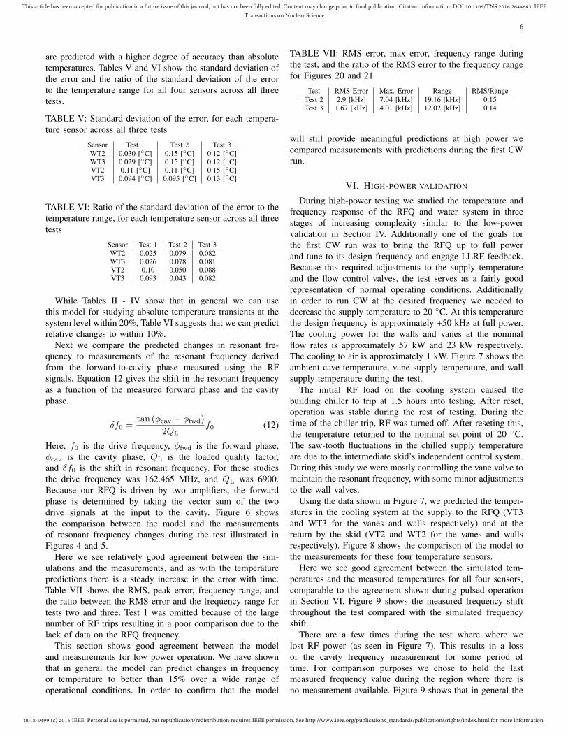
TABLE VII: RMS error, max error, frequency range duringthe test, and the ratio of the RMS error to the frequency rangefor Figures 20 and 21
Test RMS Error Max. Error Range RMS/RangeTest 2 2.9 [kHz] 7.04 [kHz] 19.16 [kHz] 0.15Test 3 1.67 [kHz] 4.01 [kHz] 12.02 [kHz] 0.14
will still provide meaningful predictions at high power wecompared measurements with predictions during the first CWrun.
VI. HIGH-POWER VALIDATION
During high-power testing we studied the temperature andfrequency response of the RFQ and water system in threestages of increasing complexity similar to the low-powervalidation in Section IV. Additionally one of the goals forthe first CW run was to bring the RFQ up to full powerand tune to its design frequency and engage LLRF feedback.Because this required adjustments to the supply temperatureand the flow control valves, the test serves as a fairly goodrepresentation of normal operating conditions. Additionallyin order to run CW at the desired frequency we needed todecrease the supply temperature to 20 ◦C. At this temperaturethe design frequency is approximately +50 kHz at full power.The cooling power for the walls and vanes at the nominalflow rates is approximately 57 kW and 23 kW respectively.The cooling to air is approximately 1 kW. Figure 7 shows theambient cave temperature, vane supply temperature, and wallsupply temperature during the test.
The initial RF load on the cooling system caused thebuilding chiller to trip at 1.5 hours into testing. After reset,operation was stable during the rest of testing. During thetime of the chiller trip, RF was turned off. After reseting this,the temperature returned to the nominal set-point of 20 ◦C.The saw-tooth fluctuations in the chilled supply temperatureare due to the intermediate skid’s independent control system.During this study we were mostly controlling the vane valve tomaintain the resonant frequency, with some minor adjustmentsto the wall valves.
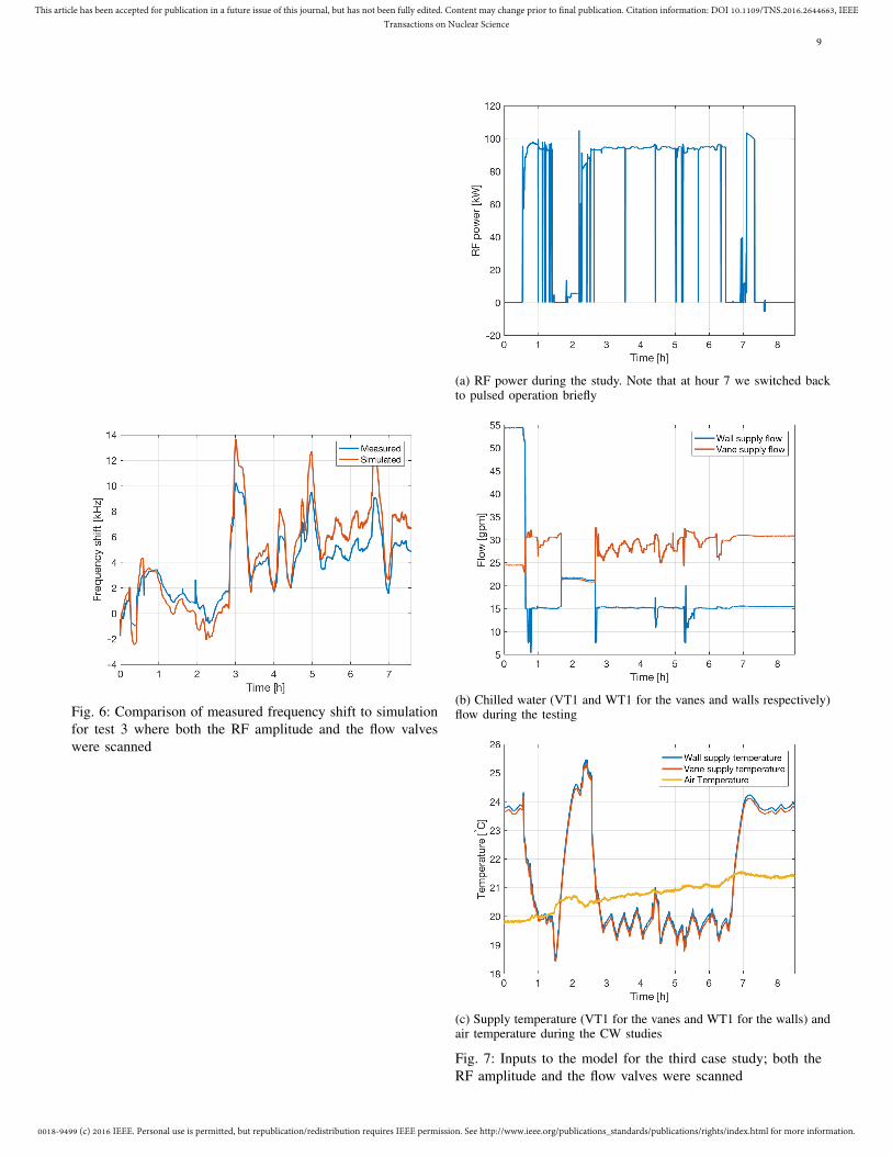
Using the data shown in Figure 7, we predicted the temper-atures in the cooling system at the supply to the RFQ (VT3and WT3 for the vanes and walls respectively) and at thereturn by the skid (VT2 and WT2 for the vanes and wallsrespectively). Figure 8 shows the comparison of the model tothe measurements for these four temperature sensors.
Here we see good agreement between the simulated tem-peratures and the measured temperatures for all four sensors,comparable to the agreement shown during pulsed operationin Section VI. Figure 9 shows the measured frequency shiftthroughout the test compared with the simulated frequencyshift.
There are a few times during the test where where welost RF power (as seen in Figure 7). This results in a lossof the cavity frequency measurement for some period oftime. For comparison purposes we chose to hold the lastmeasured frequency value during the region where there isno measurement available. Figure 9 shows that in general the
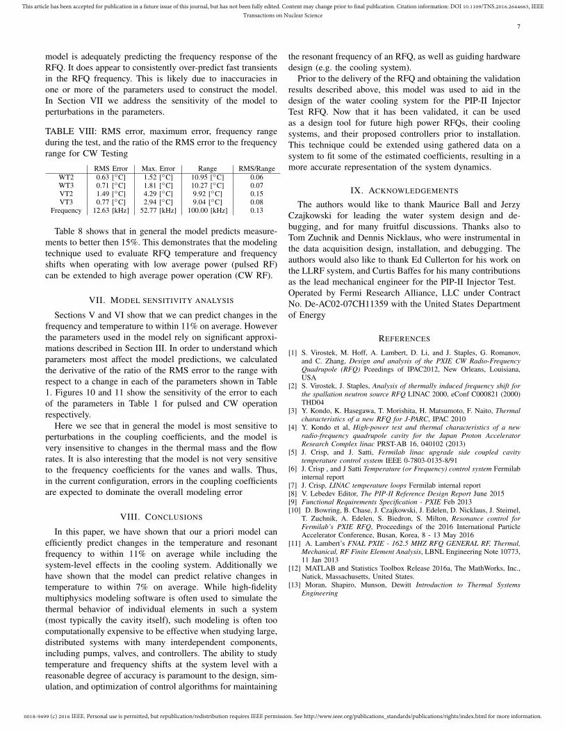
0018-9499 (c) 2016 IEEE. Personal use is permitted, but republication/redistribution requires IEEE permission. See http://www.ieee.org/publications_standards/publications/rights/index.html for more information.
This article has been accepted for publication in a future issue of this journal, but has not been fully edited. Content may change prior to final publication. Citation information: DOI 10.1109/TNS.2016.2644663, IEEETransactions on Nuclear Science
7
model is adequately predicting the frequency response of theRFQ. It does appear to consistently over-predict fast transientsin the RFQ frequency. This is likely due to inaccuracies inone or more of the parameters used to construct the model.In Section VII we address the sensitivity of the model toperturbations in the parameters.
TABLE VIII: RMS error, maximum error, frequency rangeduring the test, and the ratio of the RMS error to the frequencyrange for CW Testing
RMS Error Max. Error Range RMS/RangeWT2 0.63 [◦C] 1.52 [◦C] 10.95 [◦C] 0.06WT3 0.71 [◦C] 1.81 [◦C] 10.27 [◦C] 0.07VT2 1.49 [◦C] 4.29 [◦C] 9.92 [◦C] 0.15VT3 0.77 [◦C] 2.94 [◦C] 9.04 [◦C] 0.08
Frequency 12.63 [kHz] 52.77 [kHz] 100.00 [kHz] 0.13
Table 8 shows that in general the model predicts measure-ments to better then 15%. This demonstrates that the modelingtechnique used to evaluate RFQ temperature and frequencyshifts when operating with low average power (pulsed RF)can be extended to high average power operation (CW RF).
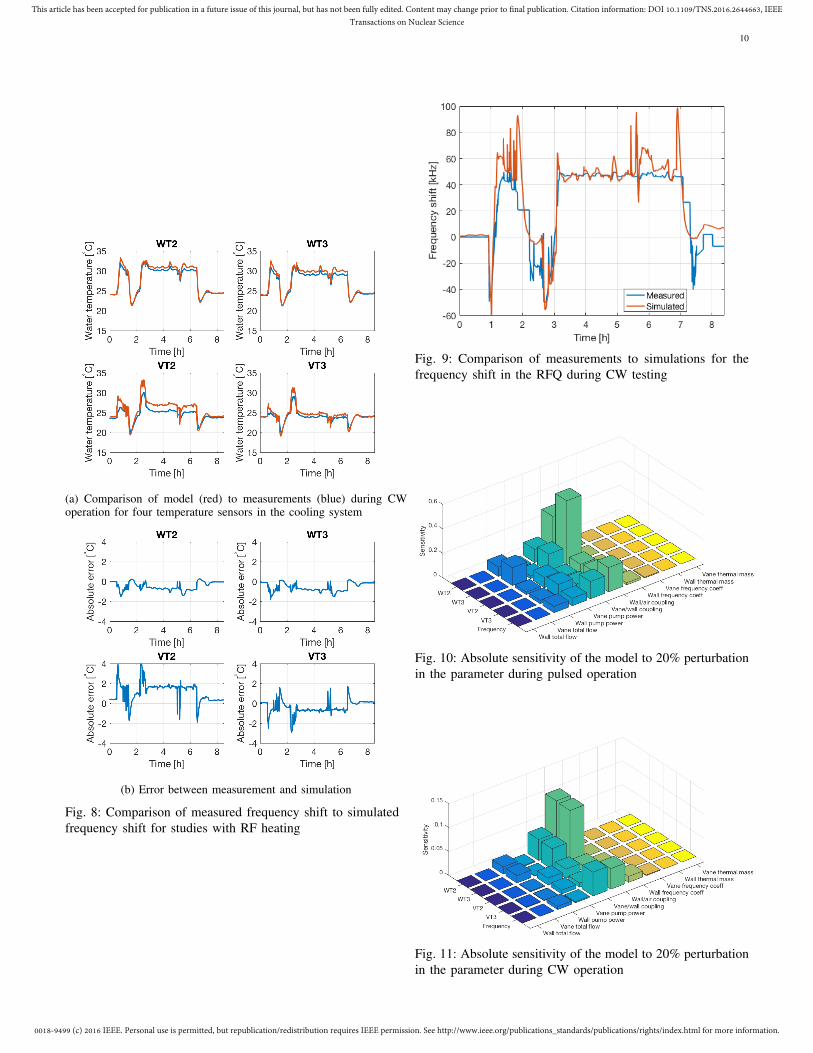
VII. MODEL SENSITIVITY ANALYSIS
Sections V and VI show that we can predict changes in thefrequency and temperature to within 11% on average. Howeverthe parameters used in the model rely on significant approxi-mations described in Section III. In order to understand whichparameters most affect the model predictions, we calculatedthe derivative of the ratio of the RMS error to the range withrespect to a change in each of the parameters shown in Table1. Figures 10 and 11 show the sensitivity of the error to eachof the parameters in Table 1 for pulsed and CW operationrespectively.
Here we see that in general the model is most sensitive toperturbations in the coupling coefficients, and the model isvery insensitive to changes in the thermal mass and the flowrates. It is also interesting that the model is not very sensitiveto the frequency coefficients for the vanes and walls. Thus,in the current configuration, errors in the coupling coefficientsare expected to dominate the overall modeling error
VIII. CONCLUSIONS
In this paper, we have shown that our a priori model canefficiently predict changes in the temperature and resonantfrequency to within 11% on average while including thesystem-level effects in the cooling system. Additionally wehave shown that the model can predict relative changes intemperature to within 7% on average. While high-fidelitymultiphysics modeling software is often used to simulate thethermal behavior of individual elements in such a system(most typically the cavity itself), such modeling is often toocomputationally expensive to be effective when studying large,distributed systems with many interdependent components,including pumps, valves, and controllers. The ability to studytemperature and frequency shifts at the system level with areasonable degree of accuracy is paramount to the design, sim-ulation, and optimization of control algorithms for maintaining
the resonant frequency of an RFQ, as well as guiding hardwaredesign (e.g. the cooling system).
Prior to the delivery of the RFQ and obtaining the validationresults described above, this model was used to aid in thedesign of the water cooling system for the PIP-II InjectorTest RFQ. Now that it has been validated, it can be usedas a design tool for future high power RFQs, their coolingsystems, and their proposed controllers prior to installation.This technique could be extended using gathered data on asystem to fit some of the estimated coefficients, resulting in amore accurate representation of the system dynamics.
IX. ACKNOWLEDGEMENTS
The authors would like to thank Maurice Ball and JerzyCzajkowski for leading the water system design and de-bugging, and for many fruitful discussions. Thanks also toTom Zuchnik and Dennis Nicklaus, who were instrumental inthe data acquisition design, installation, and debugging. Theauthors would also like to thank Ed Cullerton for his work onthe LLRF system, and Curtis Baffes for his many contributionsas the lead mechanical engineer for the PIP-II Injector Test.Operated by Fermi Research Alliance, LLC under ContractNo. De-AC02-07CH11359 with the United States Departmentof Energy
REFERENCES
[1] S. Virostek, M. Hoff, A. Lambert, D. Li, and J. Staples, G. Romanov,and C. Zhang, Design and analysis of the PXIE CW Radio-FrequencyQuadrupole (RFQ) Pceedings of IPAC2012, New Orleans, Louisiana,USA
[2] S. Virostek, J. Staples, Analysis of thermally induced frequency shift forthe spallation neutron source RFQ LINAC 2000, eConf C000821 (2000)THD04
[3] Y. Kondo, K. Hasegawa, T. Morishita, H. Matsumoto, F. Naito, Thermalcharacteristics of a new RFQ for J-PARC, IPAC 2010
[4] Y. Kondo et al, High-power test and thermal characteristics of a newradio-frequency quadrupole cavity for the Japan Proton AcceleratorResearch Complex linac PRST-AB 16, 040102 (2013)
[5] J. Crisp, and J. Satti, Fermilab linac upgrade side coupled cavitytemperature control system IEEE 0-7803-0135-8/91
[6] J. Crisp , and J Satti Temperature (or Frequency) control system Fermilabinternal report
[7] J. Crisp, LINAC temperature loops Fermilab internal report[8] V. Lebedev Editor, The PIP-II Reference Design Report June 2015[9] Functional Requirements Specification - PXIE Feb 2013[10] D. Bowring, B. Chase, J. Czajkowski, J. Edelen, D. Nicklaus, J. Steimel,
T. Zuchnik, A. Edelen, S. Biedron, S. Milton, Resonance control forFermilab’s PXIE RFQ, Proceedings of the 2016 International ParticleAccelerator Conference, Busan, Korea, 8 - 13 May 2016
[11] A. Lambert’s FNAL PXIE - 162.5 MHZ RFQ GENERAL RF, Thermal,Mechanical, RF Finite Element Analysis, LBNL Engineering Note 10773,11 Jan 2013
[12] MATLAB and Statistics Toolbox Release 2016a, The MathWorks, Inc.,Natick, Massachusetts, United States.
[13] Moran, Shapiro, Munson, Dewitt Introduction to Thermal SystemsEngineering

0018-9499 (c) 2016 IEEE. Personal use is permitted, but republication/redistribution requires IEEE permission. See http://www.ieee.org/publications_standards/publications/rights/index.html for more information.
This article has been accepted for publication in a future issue of this journal, but has not been fully edited. Content may change prior to final publication. Citation information: DOI 10.1109/TNS.2016.2644663, IEEETransactions on Nuclear Science
8
(a) RF power as a function of time throughout test 3
(b) Chilled water flow (measured at VT1 and WT1 for the vanes andwalls respectively) as a function of time throughout test 3
(c) Variation in the chilled water supply temperature (VT1 for the vanesand WT1 for the walls) and the ambient temperature during test 3
Fig. 4: Inputs to the model for the third case study; both theRF amplitude and the flow valves were scanned
(a) Comparison of measurement (blue) to simulation (red) for test 3
(b) Absolute error between measurement and simulation for test 3
Fig. 5: Comparison between measurement and simulation forthe second case study; both the RF amplitude and the flowvalves were scanned
0018-9499 (c) 2016 IEEE. Personal use is permitted, but republication/redistribution requires IEEE permission. See http://www.ieee.org/publications_standards/publications/rights/index.html for more information.
This article has been accepted for publication in a future issue of this journal, but has not been fully edited. Content may change prior to final publication. Citation information: DOI 10.1109/TNS.2016.2644663, IEEETransactions on Nuclear Science
9
Fig. 6: Comparison of measured frequency shift to simulationfor test 3 where both the RF amplitude and the flow valveswere scanned
(a) RF power during the study. Note that at hour 7 we switched backto pulsed operation briefly
(b) Chilled water (VT1 and WT1 for the vanes and walls respectively)flow during the testing
(c) Supply temperature (VT1 for the vanes and WT1 for the walls) andair temperature during the CW studies
Fig. 7: Inputs to the model for the third case study; both theRF amplitude and the flow valves were scanned
0018-9499 (c) 2016 IEEE. Personal use is permitted, but republication/redistribution requires IEEE permission. See http://www.ieee.org/publications_standards/publications/rights/index.html for more information.
This article has been accepted for publication in a future issue of this journal, but has not been fully edited. Content may change prior to final publication. Citation information: DOI 10.1109/TNS.2016.2644663, IEEETransactions on Nuclear Science
10
(a) Comparison of model (red) to measurements (blue) during CWoperation for four temperature sensors in the cooling system
(b) Error between measurement and simulation
Fig. 8: Comparison of measured frequency shift to simulatedfrequency shift for studies with RF heating
Fig. 9: Comparison of measurements to simulations for thefrequency shift in the RFQ during CW testing
Fig. 10: Absolute sensitivity of the model to 20% perturbationin the parameter during pulsed operation
Fig. 11: Absolute sensitivity of the model to 20% perturbationin the parameter during CW operation


![1.1 The Advanced Superconducting Test …lss.fnal.gov/archive/2014/pub/fermilab-pub-14-285-ad-apc.pdf1.1 The Advanced Superconducting Test Accelerator (ASTA) at Fermilab [] Elvin Harms,](https://static.fdocuments.us/doc/165x107/5b065e3d7f8b9a58148cbdf3/11-the-advanced-superconducting-test-lssfnalgovarchive2014pubfermilab-pub-14-285-ad-apcpdf11.jpg)