II INTERNATIONAL CONFERENCE ON COMPUTATIONAL BIOENGINEERINGH. Rodrigues et al. (Eds.)

Lisbon, Portugal, September 14–16, 2005

FEMUR MECHANICAL SIMULATION USINGHIGH-ORDER FE ANALYSIS WITH CONTINUOUS

MECHANICAL PROPERTIES

Royi Fedida*, Zohar Yosibash*, Charles Milgrom** and Leo Joskowicz***

* Dept. of Mech. Engrg., Ben-Gurion Univ., Beer-Sheva, Israele-mail: fedidar/zohary@bgu.ac.il

** Department of Orthopaedic Surgery, Hadassah Univ. Hospital, Jerusalem, Israel

*** School of Computer Science and Eng., Hebrew Univ., Jerusalem, Israel

Keywords: Femur, Finite Element Analysis, p-FEM, Computed Tomography.

Abstract. Femur 3D finite-element (FE) analysis based on CT data requires bothaccurate geometry representation and mechanical properties assignment. A ”structurebased” method is suggested for the reconstruction of a FE model so that the geometry isrepresented by smooth surfaces extracted from the CT data including a separating surfacebetween cortical and trabecular regions. Then, p-FE auto-mesh is generated. Within eachregion (cortical or trabecular) the heterogeneous density is described by continuous spatialfunctions that are generated using Least Mean Square (LMS) approximations based onthe CT scan data. Finally the Young modulus is evaluated continuously according to thefunctional representation of the density. Numerical investigation shows good results ofthe suggested method compared to voxel-based method. Mechanical in-vitro experimentson fresh frozen femur measuring head deflection and strains at several points is currentlyused for FE model calibration and validation.

The presented study is a first step towards a p-FEM simulation of human femursbased on CT data in order to optimize a protocol for cervical fracture surgery fixation.

Royi Fedida et al.

1 INTRODUCTION

The use of three dimensional (3-D) finite element analysis (FEA) for orthopaedic ap-plication is well accepted for more than three decades [1]. These analyses may providemedical doctors with estimation on the risk for fracture or evaluate the consequence ofmedical treatment once fracture had occurred for bones in general and for the femur inparticular. Although the bone is a complex biological tissue, the use of FEA is attractivebecause at the macro level it exhibits elastic linear behavior for loads in the normal rangeof regular daily activities [2]. The proximal femur consists of cortical (dense) and trabec-ular (cellular) tissues [3]. These constitutes were experimentally investigated to obtainhomogenized mechanical properties. In several cases bone specimens Young’s moduluswere reported as a function of bone apparent density [2,4–9]. Although constitutive mod-els of bones are better represented by an anisotropic elastic relationship, the availableinformation from CT scans are insufficient at the present to determine the numerousmaterial properties of an anisotropic domain and isotropic relationship is assumed. Theuse of Quantitative Computerized Tomography (QCT) enables the generation of accurateFE models for the human femur based on the standard DICOM format of CT scan out-put [10–15]. The accurate geometry can be obtained by an analysis of voxel coordinateswhile the Young modulus may be estimated according to the voxels intensity (given inHousfeld units - HU).

Two methods are commonly used for geometry construction and mesh generation:”voxel based” and ”structure based”. The ”voxel based” method generates a mesh of8-noded hexahedral elements, each enclosing a cubic predefined volume of the CT scanwithout any use of surfaces or solid body [1,16–18]. In the ”structure based” method, themesh is constructed on an accurate geometrical model of the bone (usually auto-meshingmethods are utilized due to the geometric complexity) [12–15, 19, 20]. Generally speak-ing, ”voxel based” models are more easily generated (via automated custom softwares)and accurate enough to estimate deflections or inside stresses, while ”structure based”models are more accurate when surface strains and stresses are of interest [1,15]. In bothmethods, inhomogeneous mechanical properties are used. Determination of element’sYoung modulus is according to an averaged value (of evaluated density and empiricalcorrelation to Young’s modulus) of the voxels enclosed in the finite element volume [21].

Because the assignment of Young’s modulus to a finite element is based on the aver-aged QCT value, a special attention should be given to the procedure. The averaged HUvalue is correlated to the bone density using linear relations [2,5, 22]. This value is thenused for Young modulus estimation usually through power-law relations as been widelyreported [4–6,8,9,12,23]. It should be noted that a QCT pixel size is of an order of 1 mm,whereas typical specimen’s dimension used for density calculation and Young modulusestimation (by experimentation) is of an order of 5 mm. Although studies on the influ-ence of the finite elements size on the results were reported [1,21], these usually considerthe computational accuracy versus meshing difficulties and computational time, yet nomechanical or biological justifications is provided for the characteristic size of elementsin use. Keyak et al. reported on hexahedral 3 mm cubic elements as a good choice for

Royi Fedida et al.

”voxel based” mesh [16, 24], yet Viceconti et al. show that further refinement can resultin an increasing error in FEA results [1]. Decreasing elements size does not lead neces-sary to convergence since both geometry and element material assignment change fromone model to the other. Furthermore, although some studies show correlation betweenFE model results and fracture load in experiments, to the best of our knowledge onlytwo studies investigate quantitatively the differences between strains computed by FEAand and these measured experimentally on a femur bone [12, 25]. In both studies onlypartial agreement is found, suggesting the need for further investigation by more reliablesimulations.

We obtain an accurate smooth representation of the bone geometry obtained by ananalysis of the QCT data, where an internal smooth surface is computed that separatesthe cortical and trabecular regions. The geometrical description in conjunction with anauto-mesher provide a p-FE mesh containing large p-elements [26]. Within each region(cortical or trabecular) the bone density is evaluated according to a moving averagemethod on HU-values. Thereafter, two different spatial functions are generated basedon LMS approximation which describe the density of the bone according to the x, y, zcoordinates (using continuous functions). Finally the Young modulus is estimated bya continuous function based on the density, without the need to assign a discrete valuefor an entire element. The motivation for this approach is that the geometry shouldbe represented as accurately as possible, and the Young modulus should be evaluatedaccording to a similar volume as the test specimens used for its estimation in actualexperimentation. Therefore, a moving average method was used so within each voxelthe QCT value is computed as an average of the QCT values in the surrounding volume(see [21]). Another point of interest is that mechanical properties are independent on theFE mesh. This requires an accurate numerical solution on bone’s surface, so validationagainst in-vitro experiments (strains measured by strain-gages on bone’s surface) willbe possible. Although the bone is known to be anisotropic and inhomogeneous, moststudies simplify these difficulties by considering an isotropic inhomogeneous material, aswe shall follow in our study and concentrate our attention in the current work on a newmethod for the geometry, mesh representation, and mechanical properties assignment forbones.

The presented work is a preliminary study in the context of a larger project in whicha p-FEM simulation of a human femur based on QCT data is investigated and comparedto experimental observations, and will be reported in a future publication.

2 GENERATING THE p-FE MODEL BASED ON QCT DATA

2.1 Mesh generation

The suggested method for the construction of the mesh is a ”structure based” method,i.e. the geometrical representation of the surfaces are as accurate as possible. The meshis generated on after a solid body is created having smooth surface representation. Thesolid body is generated by a commercial CAD software (SolidWorks 2004) according to

Royi Fedida et al.

IGES surfaces approximated by reverse engineering software (RapidForm) from the CTdata (semi-automatic procedure defines exterior surface points for that purpose). Thismodel has two distinct regions for the trabecular and cortical regions, separated by aninternal surface. The cortical region is defined using thresholds of the CT HU values andcan be defined along the diaphysis and up to a small distance above the lesser trochanter.Due to the geometry complexity of the proximal femur an auto-mesher is used obtaininghigh-order tetrahedral elements mapped by a sub-parametric function to the standardelement.

2.2 Determination of Young modulus

At the current step of our research bone mechanical properties are assumed to beisotropic with inhomogeneous Young modulus and a constant Poisson’s ratio [10, 12].Although transversely isotropic or orthotropic properties were reported [5, 6, 23], theisotropic approach is widely used especially in the trabecular bone where material prin-cipal directions are currently difficult to predict using clinical QCT protocols.

The suggested method uses a spatial field, defined by a set of 3D continuous functions,in order to assign bone heterogeneous Young’s modulus. The spatial field is evaluatedaccording to the following steps (special procedures created using MatLab 6.5 for steps1-3):

1. Data extraction: A 3D array of HU values is extracted from the CT, DICOMformat. To each member of this array we assign the coordinates of the voxelmidpoint. Then the apparent density is calculated for each voxel according to [9],or [2] with proper phantoms used.

2. Moving average: A new averaged value for apparent density is computed for eachvoxel according to the voxels located inside a 5mm cube around the voxel of inter-est (volume size can be defined according to specimen’s size used for mechanicalproperties determination). An array that covers a volume larger than the bone sizeprevents the side effects, i.e. loss of data close to the surface. False average value isprevented because averaged values are only obtained for voxels that are inside thesolid body.

3. Spatial field approximation: A 3-D polynomial functions (up to 4th degree) isevaluated based on least mean squares (LMS) so to describe the density as functionof x,y,z coordinates.

ρapp[g/cm3] =4∑

i=0

4∑

j=0

4∑

k=0

aijkxiyjzk (1)

for the femur head other spatial field is used based on spherical coordinate system.

4. Elastic modulus evaluation: The Young modulus, represented as a 3-D function, isused for each point within an element when stiffness matrices are computed (2).

Royi Fedida et al.

2.3 Loads and constrains

Loads and constrains are defined according to the specific experiment being per-formed. It is quite common to use full constrain on the distal part of a proximal femurmodel [10, 12, 17]. This constrain is according to the bone mounting in ex-vivo experi-ments.

2.4 FE solver

A p-FE code StressCheck1 Version 7.0.2 is used on a PC (Pentium 4 CPU, 2.60GHz, 1 GB RAM). The p-version solver allows high-order polynomial function spaceswhich provides exponential convergence rates in energy norm over coarse meshes (seedetails in [26]). One of the major advantages of p-FEMs over traditional h-FEMs is theability to monitor the numerical error by inspecting the convergence of the results as thepolynomial degree is increased over the mesh. In our studies the p-level for geometrybased models (having large elements and accurate boundary representation) is increasedfrom 1 to 5 and the five results at progressively larger degrees of freedom (DOFs) aremonitored.

3 THE TWO FE MODELS INVESTIGATED

3.1 A slice of a bone

As a first step the suggested method for the generation of the FE model was investi-gated numerically on a part of the bone. Three models were created based on a clinicalCT scan of a 59 years old female (140 kVp, spiral scan, 2mm slice thick with resolu-tion of 0.863 mm pixel size). A 36 mm slice of the upper diaphysis including the lessertrochanter was chosen (this section contains both trabecular and cortical bone tissues).Figure 1 shows a schematic representation of the femur location at which the slice ofinterest is analyzed. The first two (3A, 3B) were created according to the ”voxel-based”method with different element sizes (3.2 mm and 2.4 mm respectively) and an averagedvalue of evaluated voxel’s Young modulus was assigned [10]. The third model (3C) wascreated according the new suggested method.

In the elements representing the trabecular bone a heterogeneous Young modulus wasassigned according to [6]:

E[MPa] = 1904ρ1.64app (2)

with a constant value of 0.4 for Poisson’s ratio [10]. For the cortical region homogeneousYoung modulus (E = 16GPa) was used [12].

The bone slice is subjected to two different load cases: one is 700 N axial loaddistributed uniformly on the upper surface and is clamped at the bottom surface, whereas

1StressCheck is trademark of Engineering Software Research and Development, Inc, St. Louis, MO,USA

Royi Fedida et al.

the other is an axial uniform displacement of the top surface generating a 0.1% strain inthe z direction over the whole model.

Slice locationX

Y

Z

Model 3AX

Y

Z

Model 3BX

Y

Z

Model 3C

Figure 1: Different models for the bone slice model, A-B using voxel based method, Cusing spatial field method.

3.2 Proximal femur analysis accompanied by an experiment

A fresh/frozen cadaver bone (30 years old male) passed CT scan (140 kVp, 250 mAs,axial scan, 0.75 mm slice thick and resolution of 0.781 mm pixel size). Strain-gageswere positioned at four points of interest (see Fig. 2): two on femur neck (superior andinferior) and two on the femur shaft (lateral and medial). Rosette was in use for the shaftlateral point while uni-axial strain-gages were used otherwise. The bone was mountedwithin a cylindrical steel base using PMMA, and was inclined in 7◦ (typical bone positionin human body while standing) before subjected to deflection rate of 0.5 mm/min, up toload of 1500N (measurements were taken also for 15◦, 20◦ and vertical posture). A finiteelement model was generated according to the suggested method based on CT scan data.Trabecular bone Young modulus was assigned according to (2) and cortical bone Youngmodulus was assigend according to [6]:

E[MPa] = 2065ρ3.09app (3)

Clamped boundary conditions were applied to the distal part of the model and a displace-ment in the z direction was applied to the top face of femur head as in the experiment(Fig. 2).

4 RESULTS

4.1 A slice of a bone

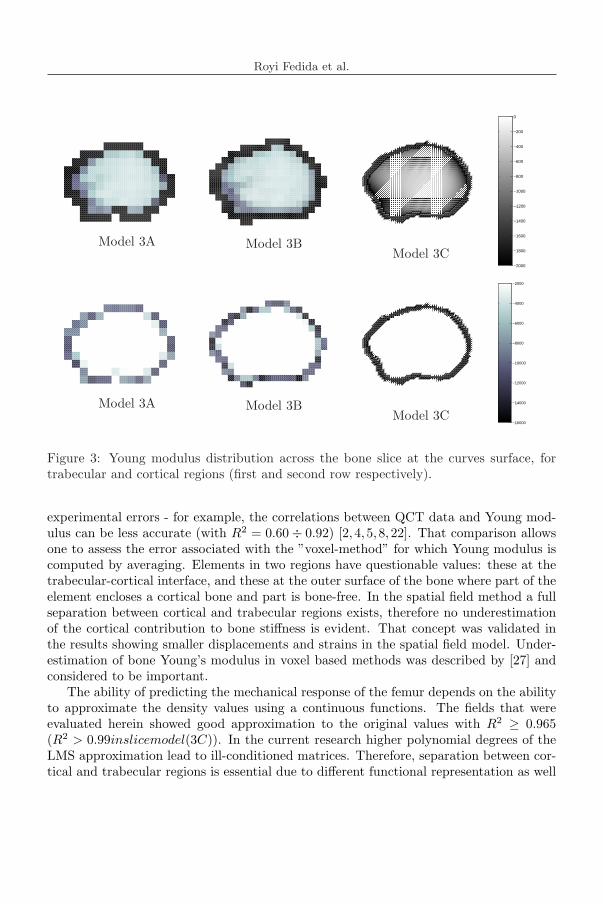
Figure 3 presents the Young modulus distribution in the model at the mid-hight plane.This distribution causes differences in the results along an ellipse inside the trabecularregion and along a medial-lateral line across the center of the bone as shown in Figure 4.

Results of the three models show qualitative agreement, i.e. same trends are seen in thedisplacement plots and in the graphs describing the displacement and strains along the

Royi Fedida et al.

(a) (b) (c)

Figure 2: (a) Fresh/frozen femur under mechanical experiment; (b) Strain-gages posi-tioning on the proximal femur: A - neck superior, B - Neck inferior, C - Shaft lateral, D- Shaft medial; (c) equivalent FE model base on CT scan data

selected curves. Yet, the spatial-field method used in conjunction with the geometrical-realistic model show almost constantly lower displacements and strains compared to the”voxel-based” methods. For example, the maximum displacement (uz) of model 3C was0.019 mm comparing to 0.022 mm according to models 3A/B (the overall displacementpattern in the three different models is presented in Figure 5). This trend is also observedin the displacements along the medial-lateral line and in the strain εzz along the ellipse(Figure 4).

4.2 Proximal femur results

Linear response was observed in all experiments performed on the proximal femur.The strain gages readings demonstrate a linear response with a linear regression fit ofR2 > 0.999. Due to large diversity in bone HU data 4 different spatial fields wereused in the FE model: one for the cortical and three for the trabecular region (lessertrochanter, greater trochanter and femoral head). That way LMS approximation regres-sion coefficient of R2 ≥ 0.965 was achieved when approximating the Young modulus bya continuous function. The FE analysis showed some difference (up to 30%) betweenthe predicted femur head displacement values and those measure experimentally. Strainprediction is much less accurate and can get to more than 100% error.

5 DISCUSSION

The maximum difference of 15% between displacement results in the numerical in-vestigation is large but in the same order of magnitude compared to the modelling and

Royi Fedida et al.

Model 3A Model 3BModel 3C

−2000

−1800

−1600

−1400

−1200

−1000

−800

−600

−400

−200

0

Model 3A Model 3BModel 3C

−16000

−14000

−12000

−10000

−8000

−6000

−4000

−2000

Figure 3: Young modulus distribution across the bone slice at the curves surface, fortrabecular and cortical regions (first and second row respectively).

experimental errors - for example, the correlations between QCT data and Young mod-ulus can be less accurate (with R2 = 0.60÷ 0.92) [2, 4, 5, 8, 22]. That comparison allowsone to assess the error associated with the ”voxel-method” for which Young modulus iscomputed by averaging. Elements in two regions have questionable values: these at thetrabecular-cortical interface, and these at the outer surface of the bone where part of theelement encloses a cortical bone and part is bone-free. In the spatial field method a fullseparation between cortical and trabecular regions exists, therefore no underestimationof the cortical contribution to bone stiffness is evident. That concept was validated inthe results showing smaller displacements and strains in the spatial field model. Under-estimation of bone Young’s modulus in voxel based methods was described by [27] andconsidered to be important.

The ability of predicting the mechanical response of the femur depends on the abilityto approximate the density values using a continuous functions. The fields that wereevaluated herein showed good approximation to the original values with R2 ≥ 0.965(R2 > 0.99inslicemodel(3C)). In the current research higher polynomial degrees of theLMS approximation lead to ill-conditioned matrices. Therefore, separation between cor-tical and trabecular regions is essential due to different functional representation as well

Royi Fedida et al.

XY

Z

Figure 4: Results along the curves inside the trabecular region at the mid-hight of theslice for the different FE models. Left: axial displacement (uz) along the medial-lateralline. Right: strain in axial direction (εzz) along the ellipse.

Model 3A Model 3B Model 3C

Figure 5: Axial displacement (Uz) for the three different bone slice models. Model 3Cshows a stiffer behavior.

as for obtaining well-conditioned matrices so to evaluate reliably the unknown coefficientsrepresenting the function. Therefore the spatial-field representation cannot be straight-forward implemented of other structure based meshing methods such as [15, 20]. Othercomplications could rise due to high density-gradients in osteoporotic region, yet againseveral fields can be used, e.g. one for the healthy trabecular region and other for theosteoporotic one.

The differences found between proximal femur analysis and the experimental mea-surements demands model improvement. That improvement is in progress and a betterfunctions for LMS approximation is sought, using other ρ − E relations including or-thotropic material properties. The prediction error reported here is better compared toerrors reported in similar studies [12,25].

Difficulties may be encountered also when trying to generate the mesh in cortical re-gions that are very thin, as in the grater trochanter, neck and the femoral head. Meshingthe thin region with 3D tetra elements is a difficult task, so the effect of neglecting thecortical shell (in the thinner regions) will be examined in the future.

The bone’s complicated geometry introduces distorted elements at several points whenan auto-mesher was used. This problem had local influence only on the strains (insignif-

Royi Fedida et al.

Figure 6: Linear regression for strain vs. force measurements (all linear regression fitsshow R2 > 0.999).

icant influence on the displacement) at several isolated points only. Although the voxel-based method is widely used, it produces results of lower accuracy, and weak singularitiesat elements edges and vertices deteriorating the convergence rate and numerical accuracydue to the abrupt change in the Young modulus.

6 SUMMARY

A new method was suggested for a more reliable simulation of the mechanical responseof bones based on an accurate representation of bone’s geometry, accurate estimationof the trabecular-cortical interface, a spatial description of the inhomogeneous Youngmodulus and high order FE analysis. This method is developed based on conceptualideas that the geometry has to be represented accurately and evaluation of mechanicalproperties should not ignore the experimental methods that were used for the reportedcorrelations between QCT and mechanical properties. The suggested method (using”structure based” mesh) shows better performance compared to the common ”voxel-based” mesh especially when realistic femur QCT data in the trabecular region is usedfor Young modulus determination, and when strains on the surface are needed to becompared to experimental observation (strain-gauges).

Currently the new method is applied for the FE analysis of a proximal femur loadedaxially. The strains at the surface are being compared to experimental results performedon the fresh/frozen femur based on which the FE model was created (using QCT scans).This comparison will be reported in a future publication. When orthotropic materialproperties will be computable from QCT scans the methodology detailed herein could beimproved with a minimal effort to provide a more realistic simulation of the mechanicalresponse of the femur.

Royi Fedida et al.

Acknowledgements: The authors thank Prof. Joyce Keyak (dept. of Orthopaedicsand dept. of Mech. & Aerospace Engrg., Univ. of California, Irvine, USA) for her helpfulremarks.

REFERENCES

[1] M. Viceconti, L. Bellingeri, L. Cristofolini, and A. Toni. A comparative study on differentmethods of automatic mesh generation of human femurs. Medical Engineering & Physics,20:1–10, 1998.

[2] T.M. Keaveny, E. Guo, E.F. Wachtel, T.A. McMahon, and W.C. Hayes. Trabecular boneexhibits fully linear elastic behavior and yields at low strains. J. Biomechanics, 27:1127–1136, 1994.

[3] S.C. Cowin and M.F. Ashby. Bone mechanics handbook. CRC Press, 2001.

[4] J.C. Lotz, T.N. Gerhart, and W.C. Hayes. Mechanical properties of metaphyseal bone inthe proximal femur. J. Biomechanics, 24:317–329, 1991.

[5] J.C. Lotz, T.N. Gerhart, and W.C. Hayes. Mechanical properties of trabecular from theproximal femur: a quantitative ct study. J. Comp. Assisted Tomography, 14(1):107–114,1990.

[6] D.C. Wirtz, N. Schiffers, T. Pandorf, K. Radermacher, D. Weichert, and R. Forst. Criticalevaluation of known bone material properties to realize anisotropic fe-simulation of theproximal femur. J. of Biomechanics, 33:1325–1330, 2000.

[7] E.F. Morgan, H.H. Bayraktar, and T.M. Keaveny. Trabecular bone modulus-density rela-tionships depend on anatomic site. J. Biomechanics, 36:897–904, 2003.

[8] T.S. Keller. Predicting the compressive mechanical behavior of bone. J. Biomechanics,27:1159–1168, 1994.

[9] J.Y. Rho, M.C. Hobatho, and R.B. Ashman. Relations of mechanical properties to densityand ct numbers in human bone. Med. Eng. Phys, 17:347–355, 1995.

[10] J.H. Keyak, S.A. Rossi, K.A. Jones, and H.B. Skinner. Prediction of femoral fracture loadusing automated finite element modeling. Journal of Biomechanics, 31:125–133, 1998.

[11] D.D. Cody, G.J. Gross, F.J. Hou, H.J. Spencer, S.A. Goldstein, and D.P. Fyhrie. Femoralstrength is better predicted by finite element models than qct and dxa. J. Biomechanics,32:1013–1020, 1999.

[12] J.C. Lotz, E.J. Cheal, and W.C Hayes. Fracture prediction for the proximal femur usingfinite element models: part 1 - linear analysis. J. of Biomechanical Eng., 113:353–360, 1991.

[13] B. Mertz, P. Niederer, R. Muller, and P. Ruegsegger. Automated finite element analysis ofexcised human femura based on precision-qct. J. Biomechanical Eng., 118:387–390, 1996.

[14] D.C. Wirtz, T. Pandorf, F. Portheine, K. Radermacher, N. Schiffers, A. Prescher, D. We-ichert, and U.N. Fritz. Concept and development of an orthotropic fe model of the proximalfemur. J. of Biomechanics, 36:289–293, 2003.

[15] B. Couteau, Y. Payan, and S. Lavallee. The mesh-matching algorithm: an automatic 3dmesh generator for finite element structures. J. Biomechanics, 33:1005–1009, 2000.

Royi Fedida et al.

[16] J.H. Keyak, J.M. Meagher, H.B. Skinner, and Jr C. D. Mote. Automated three-dimensionalfinite element modelling of bone: a new method. Journal of Biomedical Engineering, 12:389–397, 1990.

[17] D.D. Cody, D.A. McCubbrey, G.W. Divine, G.J. Gross, and S.A. Goldstein. Predictivevalue of proximal femural bone densiometry in detrmining local orthogonal material prop-erties. J. Biomechanics, 29:753–761, 1996.

[18] J.C. Fox, A. Gupta, G. Blumenkrantz, H.H. Bayraktar, and T.M. Keaveny. Role of elasticanisotropy and failure criterion in femoral fracture strength predictions. Trans. OrthopaedicResearch Society, page 520, 2004.

[19] A.S. Marom and M.J. Linden. Computer aided stress analysis of long bones utilizingcomputed tomography. J. Biomechanics, 23:399–404, 1990.

[20] M. Viceconti, M. Davinelli, F. Taddei, and A. Cappello. Automatic generation of accuratesubject-specific bone finite element models to be used in clinical studies. J. Biomechanics,37:1597–1605, 2004.

[21] F. Taddei, A. Pancanti, and M. Viceconti. An improved method for the automatic mappingof computed tomography numbers onto finite element models. Medical Engineering &Physics, 26:61–69, 2004.

[22] S.I. Esses, J.C. Lotz, and W.C. Hayes. Biomechanical properties of the proximal femurdetermined in vitro by single-energy quantitative computed tomography. J. of bone andmineral research, 4:715–722, 1989.

[23] G. Yang, J. Kabel, B. Van Riertbergen, A. Odgaard, R. Huiskes, and S.C. Cowin. Theanisotropic hooke’s law for cancellous bone and wood. J. of Elasticity, 53:125–146, 1999.

[24] J.H. Keyak and H.B. Skinner. Three-dimensional finite element modelling of bone: effectof element size. Journal of Biomedical Engineering, 14:483–489, 1992.

[25] J.H. Keyak, M.G. Fourkas, J.M. Meagher, and Skinner H.B. Validation of automatedmethod of three-dimensional finite element modelling of bone. Journal of Biomedical En-gineering, 15:505–509, 1993.

[26] B. A. Szabo and I. Babuska. Finite Element Analysis. John-Wiley, New York, 1991.

[27] C. Zannoni, R. Mantovani, and M. Viceconti. Material properties assignment to finiteelement models of bone structure: a new method. Med. Eng. Phys, 20:735–740, 1998.