
FEM/BEM NOTES - TU Wienmagnet.atp.tuwien.ac.at/suess/cp/download/fembemnotes.pdf · Chapter 1...
77
FEM/BEM NOTES http://www.bioeng.auckland.ac.nz/cmiss/fembemnotes/fembemnotes.pdf Bioengineering Institute The University of Auckland New Zealand February 9, 2005 c Copyright 1997- Bioengineering Institute The University of Auckland
Transcript of FEM/BEM NOTES - TU Wienmagnet.atp.tuwien.ac.at/suess/cp/download/fembemnotes.pdf · Chapter 1...
FEM/BEM NOTEShttp://www.bioeng.auckland.ac.nz/cmiss/fembemnotes/fembemnotes.pdf
Bioengineering InstituteThe University of Auckland
New Zealand
February 9, 2005
c Copyright 1997-Bioengineering Institute
The University of Auckland

Contents
1 Finite Element Basis Functions 11.1 Representing a One-Dimensional Field . . . . . . . . . . . . . . .. . . . . . . . . 11.2 Linear Basis Functions . . . . . . . . . . . . . . . . . . . . . . . . . . . .. . . . 21.3 Basis Functions as Weighting Functions . . . . . . . . . . . . . .. . . . . . . . . 41.4 Quadratic Basis Functions . . . . . . . . . . . . . . . . . . . . . . . . .. . . . . 71.5 Two- and Three-Dimensional Elements . . . . . . . . . . . . . . . .. . . . . . . 71.6 Higher Order Continuity . . . . . . . . . . . . . . . . . . . . . . . . . . .. . . . 101.7 Triangular Elements . . . . . . . . . . . . . . . . . . . . . . . . . . . . . .. . . . 141.8 Curvilinear Coordinate Systems . . . . . . . . . . . . . . . . . . . .. . . . . . . 161.9 CMISS Examples . . . . . . . . . . . . . . . . . . . . . . . . . . . . . . . . . . .20
2 Steady-State Heat Conduction 232.1 One-Dimensional Steady-State Heat Conduction . . . . . . .. . . . . . . . . . . 23
2.1.1 Integral equation . . . . . . . . . . . . . . . . . . . . . . . . . . . . . .. 242.1.2 Integration by parts . . . . . . . . . . . . . . . . . . . . . . . . . . . .. . 242.1.3 Finite element approximation . . . . . . . . . . . . . . . . . . . .. . . . 252.1.4 Element integrals . . . . . . . . . . . . . . . . . . . . . . . . . . . . . .. 262.1.5 Assembly . . . . . . . . . . . . . . . . . . . . . . . . . . . . . . . . . . . 272.1.6 Boundary conditions . . . . . . . . . . . . . . . . . . . . . . . . . . . .. 292.1.7 Solution . . . . . . . . . . . . . . . . . . . . . . . . . . . . . . . . . . . . 292.1.8 Fluxes . . . . . . . . . . . . . . . . . . . . . . . . . . . . . . . . . . . . . 29
2.2 Anx-Dependent Source Term . . . . . . . . . . . . . . . . . . . . . . . . . . . . 302.3 The Galerkin Weight Function Revisited . . . . . . . . . . . . . .. . . . . . . . . 312.4 Two and Three-Dimensional Steady-State Heat Conduction . . . . . . . . . . . . . 322.5 Basis Functions - Element Discretisation . . . . . . . . . . . .. . . . . . . . . . . 342.6 Integration . . . . . . . . . . . . . . . . . . . . . . . . . . . . . . . . . . . . .. . 362.7 Assemble Global Equations . . . . . . . . . . . . . . . . . . . . . . . . .. . . . . 372.8 Gaussian Quadrature . . . . . . . . . . . . . . . . . . . . . . . . . . . . . .. . . 392.9 CMISS Examples . . . . . . . . . . . . . . . . . . . . . . . . . . . . . . . . . . .42
3 The Boundary Element Method 433.1 Introduction . . . . . . . . . . . . . . . . . . . . . . . . . . . . . . . . . . . .. . 433.2 The Dirac-Delta Function and Fundamental Solutions . . .. . . . . . . . . . . . . 43
3.2.1 Dirac-Delta function . . . . . . . . . . . . . . . . . . . . . . . . . . .. . 433.2.2 Fundamental solutions . . . . . . . . . . . . . . . . . . . . . . . . . .. . 45
ii CONTENTS
3.3 The Two-Dimensional Boundary Element Method . . . . . . . . .. . . . . . . . . 483.4 Numerical Solution Procedures for the Boundary Integral Equation . . . . . . . . . 533.5 Numerical Evaluation of Coefficient Integrals . . . . . . . .. . . . . . . . . . . . 553.6 The Three-Dimensional Boundary Element Method . . . . . . .. . . . . . . . . . 573.7 A Comparison of the FE and BE Methods . . . . . . . . . . . . . . . . . .. . . . 583.8 More on Numerical Integration . . . . . . . . . . . . . . . . . . . . . .. . . . . . 60
3.8.1 Logarithmic quadrature and other special schemes . . .. . . . . . . . . . 603.8.2 Special solutions . . . . . . . . . . . . . . . . . . . . . . . . . . . . . .. 61
3.9 The Boundary Element Method Applied to other Elliptic PDEs . . . . . . . . . . . 613.10 Solution of Matrix Equations . . . . . . . . . . . . . . . . . . . . . .. . . . . . . 613.11 Coupling the FE and BE techniques . . . . . . . . . . . . . . . . . . .. . . . . . 623.12 Other BEM techniques . . . . . . . . . . . . . . . . . . . . . . . . . . . . .. . . 64
3.12.1 Trefftz method . . . . . . . . . . . . . . . . . . . . . . . . . . . . . . . .643.12.2 Regular BEM . . . . . . . . . . . . . . . . . . . . . . . . . . . . . . . . . 64
3.13 Symmetry . . . . . . . . . . . . . . . . . . . . . . . . . . . . . . . . . . . . . . .653.14 Axisymmetric Problems . . . . . . . . . . . . . . . . . . . . . . . . . . .. . . . 673.15 Infinite Regions . . . . . . . . . . . . . . . . . . . . . . . . . . . . . . . . .. . . 693.16 Appendix: Common Fundamental Solutions . . . . . . . . . . . .. . . . . . . . . 72
3.16.1 Two-Dimensional equations . . . . . . . . . . . . . . . . . . . . .. . . . 723.16.2 Three-Dimensional equations . . . . . . . . . . . . . . . . . . .. . . . . 723.16.3 Axisymmetric problems . . . . . . . . . . . . . . . . . . . . . . . . .. . 73
3.17 CMISS Examples . . . . . . . . . . . . . . . . . . . . . . . . . . . . . . . . . .. 73
4 Transient Heat Conduction 754.1 Introduction . . . . . . . . . . . . . . . . . . . . . . . . . . . . . . . . . . . .. . 754.2 Finite Differences . . . . . . . . . . . . . . . . . . . . . . . . . . . . . . .. . . . 75
4.2.1 Explicit Transient Finite Differences . . . . . . . . . . . .. . . . . . . . . 754.2.2 Von Neumann Stability Analysis . . . . . . . . . . . . . . . . . . .. . . . 774.2.3 Higher Order Approximations . . . . . . . . . . . . . . . . . . . . .. . . 78
4.3 The Transient Advection-Diffusion Equation . . . . . . . . .. . . . . . . . . . . 794.4 Mass lumping . . . . . . . . . . . . . . . . . . . . . . . . . . . . . . . . . . . . .824.5 CMISS Examples . . . . . . . . . . . . . . . . . . . . . . . . . . . . . . . . . . .84
5 Linear Elasticity 875.1 Introduction . . . . . . . . . . . . . . . . . . . . . . . . . . . . . . . . . . . .. . 875.2 Truss Elements . . . . . . . . . . . . . . . . . . . . . . . . . . . . . . . . . . .. 885.3 Beam Elements . . . . . . . . . . . . . . . . . . . . . . . . . . . . . . . . . . . .915.4 Plane Stress Elements . . . . . . . . . . . . . . . . . . . . . . . . . . . . .. . . . 93
5.4.1 Notes on calculating nodal loads . . . . . . . . . . . . . . . . . .. . . . . 955.5 Three-Dimensional Elasticity . . . . . . . . . . . . . . . . . . . . .. . . . . . . . 96
5.5.1 Weighted Residual Integral Equation . . . . . . . . . . . . . .. . . . . . 975.5.2 The Principle of Virtual Work . . . . . . . . . . . . . . . . . . . . .. . . 985.5.3 The Finite Element Approximation . . . . . . . . . . . . . . . . .. . . . 99
5.6 Linear Elasticity with Boundary Elements . . . . . . . . . . . .. . . . . . . . . . 1015.7 Fundamental Solutions . . . . . . . . . . . . . . . . . . . . . . . . . . . .. . . . 103

CONTENTS iii
5.8 Boundary Integral Equation . . . . . . . . . . . . . . . . . . . . . . . .. . . . . . 1055.9 Body Forces (and Domain Integrals in General) . . . . . . . . .. . . . . . . . . . 1085.10 CMISS Examples . . . . . . . . . . . . . . . . . . . . . . . . . . . . . . . . . .. 110
6 Modal Analysis 1116.1 Introduction . . . . . . . . . . . . . . . . . . . . . . . . . . . . . . . . . . . .. . 1116.2 Free Vibration Modes . . . . . . . . . . . . . . . . . . . . . . . . . . . . . .. . . 1116.3 An Analytic Example . . . . . . . . . . . . . . . . . . . . . . . . . . . . . . .. . 1136.4 Proportional Damping . . . . . . . . . . . . . . . . . . . . . . . . . . . . .. . . 1146.5 CMISS Examples . . . . . . . . . . . . . . . . . . . . . . . . . . . . . . . . . . .115
7 Domain Integrals in the BEM 1177.1 Achieving a Boundary Integral Formulation . . . . . . . . . . .. . . . . . . . . . 1177.2 Removing Domain Integrals due to Inhomogeneous Terms . .. . . . . . . . . . . 118
7.2.1 The Galerkin Vector technique . . . . . . . . . . . . . . . . . . . .. . . . 1187.2.2 The Monte Carlo method . . . . . . . . . . . . . . . . . . . . . . . . . . .1197.2.3 Complementary Function-Particular Integral method. . . . . . . . . . . . 120
7.3 Domain Integrals Involving the Dependent Variable . . . .. . . . . . . . . . . . . 1207.3.1 The Perturbation Boundary Element Method . . . . . . . . . .. . . . . . 1217.3.2 The Multiple Reciprocity Method . . . . . . . . . . . . . . . . . .. . . . 1227.3.3 The Dual Reciprocity Boundary Element Method . . . . . . .. . . . . . . 124
8 The BEM for Parabolic PDES 1358.1 Time-Stepping Methods . . . . . . . . . . . . . . . . . . . . . . . . . . . .. . . 135
8.1.1 Coupled Finite Difference - Boundary Element Method .. . . . . . . . . . 1358.1.2 Direct Time-Integration Method . . . . . . . . . . . . . . . . . .. . . . . 137
8.2 Laplace Transform Method . . . . . . . . . . . . . . . . . . . . . . . . . .. . . . 1388.3 The DR-BEM For Transient Problems . . . . . . . . . . . . . . . . . . .. . . . . 1398.4 The MRM for Transient Problems . . . . . . . . . . . . . . . . . . . . . .. . . . 140
Bibliography 143
Index 147

Chapter 1
Finite Element Basis Functions
1.1 Representing a One-Dimensional Field
Consider the problem of finding a mathematical expressionu (x) to represent a one-dimensionalfield e.g.,measurements of temperatureu against distancex along a bar, as shown in Figure 1.1a.
+ + ++++
++
+ + xx
u u
(a)
++
+
(b)
++
++
+
+
+
++
++
+
++ + +
+
FIGURE 1.1: (a) Temperature distributionu (x) along a bar. The points are the measuredtemperatures. (b) A least-squares polynomial fit to the data, showing the unacceptable oscillation
between data points.
One approach would be to use a polynomial expressionu (x) = a + bx + cx2 + dx3 + : : :and to estimate the values of the parametersa, b, c andd from a least-squares fit to the data. Asthe degree of the polynomial is increased the data points arefitted with increasing accuracy andpolynomials provide a very convenient form of expression because they can be differentiated andintegrated readily. For low degree polynomials this is a satisfactory approach, but if the polynomialorder is increased further to improve the accuracy of fit a problem arises: the polynomial can bemade to fit the data accurately, but it oscillates unacceptably between the data points, as shown inFigure 1.1b.
To circumvent this, while retaining the advantages of low degree polynomials, we divide thebar into three subregions and use low order polynomials overeach subregion - calledelements. Forlater generality we also introduce a parameters which is a measure of distance along the bar.u isplotted as a function of this arclength in Figure 1.2a. Figure 1.2b shows three linear polynomialsin s fitted by least-squares separately to the data in each element.
2 FINITE ELEMENT BASIS FUNCTIONS
+
+++
+
++
++
+
+
(b)s
u
s
u(a)
++
+ + ++
++
++
++
++ +
+
++
+
++
FIGURE 1.2: (a) Temperature measurements replotted against arclength parameters. (b) Thes
domain is divided into three subdomains,elements, and linear polynomials are independently fittedto the data in each subdomain.
1.2 Linear Basis Functions
A new problem has now arisen in Figure 1.2b: the piecewise linear polynomials are not continuousin u across the boundaries between elements. One solution wouldbe to constrain the parametersa,b, c etc. to ensure continuity ofu across the element boundaries, but a better solution is to replacethe parametersa andb in the first element with parametersu1 andu2, which are the values ofu atthe two ends of that element. We then define a linear variationbetween these two values byu (�) = (1� �)u1 + �u2
where�(0 � � � 1) is a normalized measure of distance along the curve.We define '1 (�) = 1� �'2 (�) = �
such that u (�) = '1 (�)u1 + '2 (�)u2
and refer to these expressions as thebasisfunctions associated with thenodalparametersu1 andu2. The basis functions'1 (�) and'2 (�) are straight lines varying between0 and1 as shown inFigure 1.3.
It is convenient always to associate the nodal quantityun with element noden and to map thetemperatureU� defined atglobal node� onto local noden of elemente by using a connectivitymatrix�(n; e) i.e., un = U�(n;e)
where�(n; e) = global node number of local noden of elemente. This has the advantage that the

1.2 LINEAR BASIS FUNCTIONS 3
1 �
110
'2 (�)'1 (�)
� 10
1
FIGURE 1.3: Linear basis functions'1 (�) = 1� � and'2 (�) = �.
interpolation u (�) = '1 (�)u1 + '2 (�)u2
holds for any element provided thatu1 andu2 are correctly identified with their global counterparts,as shown in Figure 1.4. Thus, in the first element
node4 xu1 u2 �
node3
element1 element2 element3
node1 node2u1
10 1 0 1 0
u2 �u1 u2 �U1
nodes:
global nodes:
element
U3 U4U2
FIGURE 1.4: The relationship between global nodes and element nodes.u (�) = '1 (�)u1 + '2 (�)u2 (1.1)
with u1 = U1 andu2 = U2.In the second elementu is interpolated byu (�) = '1 (�)u1 + '2 (�)u2 (1.2)
with u1 = U2 andu2 = U3, since the parameterU2 is shared between the first and second elements
4 FINITE ELEMENT BASIS FUNCTIONS
the temperature fieldu is implicitly continuous. Similarly, in the third elementu is interpolated byu (�) = '1 (�)u1 + '2 (�)u2 (1.3)
with u1 = U3 andu2 = U4, with the parameterU3 being shared between the second and thirdelements. Figure 1.6 shows the temperature field defined by the three interpolations (1.1)–(1.3).
++
++
++
+ +
+
node1node2
u
snode4
+
+
+
node3
+
element2 element3element1+
+
+
FIGURE 1.5: Temperature measurements fitted with nodal parametersand linear basis functions.The fitted temperature field is now continuous across elementboundaries.
1.3 Basis Functions as Weighting Functions
It is useful to think of the basis functions as weighting functions on the nodal parameters. Thus, inelement 1
at � = 0 u (0) = (1� 0)u1 + 0u2 = u1
which is the value ofu at the left hand end of the element and has no dependence onu2
at � = 14 u�14� = �1� 14� u1 + 14u2 = 34u1 + 14u2
which depends onu1 andu2, but is weighted more towardsu1 thanu2
at � = 12 u�12� = �1� 12� u1 + 12u2 = 12u1 + 12u2
which depends equally onu1 andu2
at � = 34 u�34� = �1� 34� u1 + 34u2 = 14u1 + 34u2

1.3 BASIS FUNCTIONS AS WEIGHTING FUNCTIONS 5
which depends onu1 andu2 but is weighted more towardsu2 thanu1
at � = 1 u (1) = (1� 1)u1 + 1u2 = u2
which is the value ofu at the right hand end of the region and has no dependence onu1.Moreover, these weighting functions can be considered asglobal functions, as shown in Fig-
ure 1.6, where the weighting functionwn associated with global noden is constructed from thebasis functions in the elements adjacent to that node.
(a)
w3s
ss
sw4
(b)
(c)
(d)
w1w2
FIGURE 1.6: (a): : : (d) The weighting functionswn associated with the global nodesn = 1 : : : 4,respectively. Notice the linear fall off in the elements adjacent to a node. Outside the immediately
adjacent elements, the weighting functions are defined to bezero.
For example,w2 weights the global parameterU2 and the influence ofU2 falls off linearly inthe elements on either side of node 2.
We now have a continuous piecewise parametric description of the temperature fieldu (�) butin order to defineu (x) we need to define the relationship betweenx and� for each element. Aconvenient way to do this is to definex as an interpolation of the nodal values ofx.
For example, in element 1 x (�) = '1 (�)x1 + '2 (�)x2 (1.4)
and similarly for the other two elements. The dependence of temperature onx, u (x), is therefore
6 FINITE ELEMENT BASIS FUNCTIONS
defined by the parametric expressionsu (�) =Xn 'n (�)unx(�) =Xn 'n (�)xnwhere summation is taken over all element nodes (in this caseonly 2) and the parameter� (the“element coordinate”) links temperatureu to physical positionx. x (�) provides the mappingbetween the mathematical space0 � � � 1 and the physical spacex1 � x � x2, as illustrated inFigure 1.7.
u1
u (x) at � = 0:200
x2u2
� = 0:2� = 0:2 �
��
x1
x2 x
ux
u1
u1u20 x11
FIGURE 1.7: Illustrating howx andu are related through the normalized element coordinate�.The values ofx (�) andu (�) are obtained from a linear interpolation of the nodal variables and
then plotted asu (x). The points at� = 0:2 are emphasized.

1.4 QUADRATIC BASIS FUNCTIONS 7
1.4 Quadratic Basis Functions
The essential property of the basis functions defined above is that the basis function associatedwith a particular node takes the value of1 when evaluated at that node and is zero at every othernode in the element (only one other in the case of linear basisfunctions). This ensures the linearindependence of the basis functions. It is also the key to establishing the form of the basis functionsfor higher order interpolation. For example, a quadratic variation of u over an element requiresthree nodal parametersu1, u2 andu3u (�) = '1 (�)u1 + '2 (�)u2 + '3 (�)u3 (1.5)
The quadratic basis functions are shown, with their mathematical expressions, in Figure 1.8. Noticethat since'1 (�) must be zero at� = 0:5 (node2), '1 (�) must have a factor(� � 0:5) and since itis also zero at� = 1 (node3), another factor is(� � 1). Finally, since'1 (�) is 1 at � = 0 (node1)we have'1 (�) = 2 (� � 1) (� � 0:5). Similarly for the other two basis functions.
��1
10
0'3 (�)
(c)'3 (�) = 2� (� � 0:5)
(a)'1 (�) = 2 (� � 1) (� � 0:5) (b)'2 (�) = 4� (1� �)'2 (�)
110:5
0:5�01
1'1 (�)
0:5
FIGURE 1.8: One-dimensional quadratic basis functions.
1.5 Two- and Three-Dimensional Elements
Two-dimensional bilinear basis functions are constructedfrom the products of the above one-dimensional linear functions as follows
8 FINITE ELEMENT BASIS FUNCTIONS
Let u (�1; �2) = '1 (�1; �2)u1 + '2 (�1; �2)u2 + '3 (�1; �2) u3 + '4 (�1; �2) u4where '1 (�1; �2) = (1� �1) (1� �2)'2 (�1; �2) = �1 (1� �2)'3 (�1; �2) = (1� �1) �2'4 (�1; �2) = �1�2 (1.6)
Note that'1 (�1; �2) = '1 (�1)'1 (�2) where'1 (�1) and'1 (�2) are the one-dimensional linearbasis functions. Similarly,'2 (�1; �2) = '2 (�1)'1 (�2) : : : etc.
These four bilinear basis functions are illustrated in Figure 1.9.
�2�1node4�1
node3
node2
0 1
�2'1 '3
'2 '4
1
10
node1 �20 �1
�2�1
FIGURE 1.9: Two-dimensional bilinear basis functions.
Notice that'n (�1; �2) is 1 at noden and zero at the other three nodes. This ensures that thetemperatureu (�1; �2) receives a contribution from each nodal parameterun weighted by'n (�1; �2)
and that whenu (�1; �2) is evaluated at noden it takes on the valueun.As before the geometry of the element is defined in terms of thenode positions(xn; yn), n =

1.5 TWO- AND THREE-DIMENSIONAL ELEMENTS 91; : : : ; 4 by x =Xn 'n (�1; �2)xny =Xn 'n (�1; �2) yn
which provide the mapping between the mathematical space(�1; �2) (where0 � �1; �2 � 1) andthe physical space(x; y).
Higher order 2D basis functions can be similarly constructed from products of the appropriate1D basis functions. For example, a six-noded (see Figure 1.10) quadratic-linear element (quadraticin �1 and linear in�2) would have u = 6Xn=1 'n (�1; �2)un
where'1 (�1; �2) = 2 (�1 � 1) (�1 � 0:5) (1� �2) '2 (�1; �2) = 4�1 (1� �1) (1� �2) (1.7)'3 (�1; �2) = 2�1 (�1 � 0:5) (1� �2) '4 (�1; �2) = 2 (�1 � 1) (�1 � 0:5) �2 (1.8)'5 (�1; �2) = 4�1 (1� �1) �2 '6 (�1; �2) = 2�1 (�1 � 0:5) �2 (1.9)
�10 0:5 101 �2 654
321
FIGURE 1.10: A6-node quadratic-linear element (node numbers circled).
Three-dimensional basis functions are formed similarly,e.g.,a trilinear element basis has eightnodes (see Figure 1.11) with basis functions'1 (�1; �2; �3) = (1� �1) (1� �2) (1� �3) '2 (�1; �2; �3) = �1 (1� �2) (1� �3) (1.10)'3 (�1; �2; �3) = (1� �1) �2 (1� �3) '4 (�1; �2; �3) = �1�2 (1� �3) (1.11)'5 (�1; �2; �3) = (1� �1) (1� �2) �3 '6 (�1; �2; �3) = �1 (1� �2) �3 (1.12)'7 (�1; �2; �3) = (1� �1) �2�3 '8 (�1; �2; �3) = �1�2�3 (1.13)
10 FINITE ELEMENT BASIS FUNCTIONS
�1�2
�31
532 4
876
FIGURE 1.11: An8-node trilinear element.
1.6 Higher Order Continuity
All the basis functions mentioned so far areLagrange1 basis functions and provide continuity ofu
across element boundaries but not higher order continuity.Sometimes it is desirable to use basisfunctions which also preserve continuity of the derivativeof u with respect to� across elementboundaries. A convenient way to achieve this is by defining two additional nodal parameters�dud��n. The basis functions are chosen to ensure thatdud� �����=0 = �dud��1 = u01 and
dud� �����=1 = �dud��2 = u02
and sinceun is shared between adjacent elements derivative continuityis ensured. Since the num-ber of element parameters is 4 the basis functions must be cubic in �. To derive these cubicHermite2 basis functions let u (�) = a+ b� + c�2 + d�3;dud� = b + 2c� + 3d�2;
1Joseph-Louis Lagrange (1736-1813).2Charles Hermite (1822-1901).
1.6 HIGHER ORDER CONTINUITY 11
and impose the constraints u (0) = a = u1u (1) = a+ b+ c+ d = u2dud� (0) = b = u01dud� (1) = b+ 2c+ 3d = u02
These four equations in the four unknownsa, b, c andd are solved to givea = u1b = u01c = 3u2 � 3u1 � 2u01 � u02d = u01 + u02 + 2u1 � 2u2
Substitutinga, b, c andd back into the original cubic then givesu (�) = u1 + u01� + (3u2 � 3u1 � 2u01 � u02) �2 + (u01 + u02 + 2u1 � 2u2) �3
or, rearranging, u (�) = 01 (�)u1 + 11 (�)u01 +02 (�)u2 +12 (�)u02 (1.14)
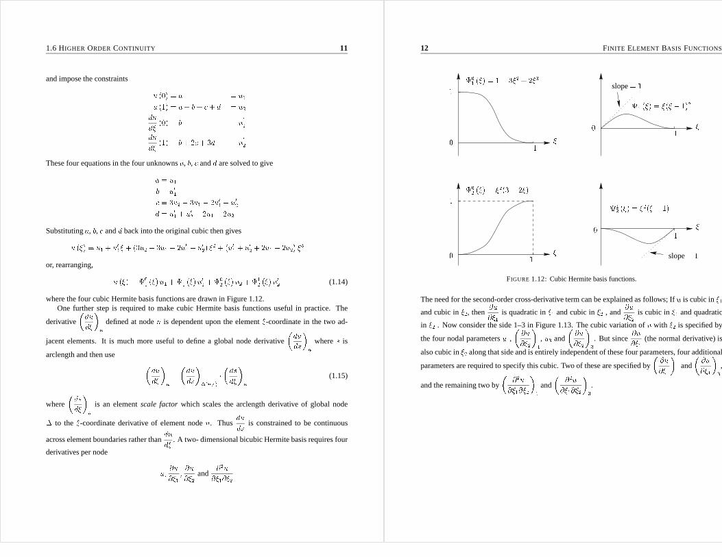
where the four cubic Hermite basis functions are drawn in Figure 1.12.One further step is required to make cubic Hermite basis functions useful in practice. The
derivative
�dud��n defined at noden is dependent upon the element�-coordinate in the two ad-
jacent elements. It is much more useful to define a global nodederivative
�duds�n wheres is
arclength and then use �dud��n = �duds��(n;e) � �dsd��n (1.15)
where
�dsd��n is an elementscale factorwhich scales the arclength derivative of global node� to the �-coordinate derivative of element noden. Thus
duds is constrained to be continuous
across element boundaries rather than
dud� . A two- dimensional bicubic Hermite basis requires four
derivatives per node u; @u@�1 ; @u@�2 and
@2u@�1@�2
12 FINITE ELEMENT BASIS FUNCTIONS1
10
11
01 (�) = 1� 3�2 + 2�3 11 (�) = �(� � 1)2
02 (�) = �2(3� 2�) 12 (�) = �2(� � 1)
0 � �
� �
slope= 1
10 1
0slope= 1
FIGURE 1.12: Cubic Hermite basis functions.
The need for the second-order cross-derivative term can be explained as follows; Ifu is cubic in�1
and cubic in�2, then
@u@�1 is quadratic in�1 and cubic in�2 , and
@u@�2 is cubic in�1 and quadratic
in �2 . Now consider the side 1–3 in Figure 1.13. The cubic variation of u with �2 is specified by
the four nodal parametersu1, � @u@�2�1, u3 and
� @u@�2�3. But since
@u@�1 (the normal derivative) is
also cubic in�2 along that side and is entirely independent of these four parameters, four additional
parameters are required to specify this cubic. Two of these are specified by
� @u@�1�1 and
� @u@�1�3,and the remaining two by
� @2u@�1@�2�1 and
� @2u@�1@�2�3.
1.6 HIGHER ORDER CONTINUITY 13
node4node3
�1
node2
�2
node1� @u@�1�1� @u@�1�3
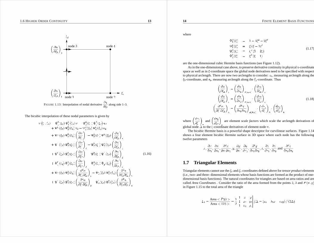
FIGURE 1.13: Interpolation of nodal derivative
@u@�1 along side 1–3.
The bicubic interpolation of these nodal parameters is given byu (�1; �2) = 01 (�1)01 (�2) u1 +02 (�1)01 (�2) u2+01 (�1)02 (�2) u3 +02 (�1)02 (�2) u4+11 (�1)01 (�2)� @u@�1�1 +12 (�1)01 (�2)� @u@�1�2+11 (�1)02 (�2)� @u@�1�3 +12 (�1)02 (�2)� @u@�1�4+01 (�1)11 (�2)� @u@�2�1 +02 (�1)11 (�2)� @u@�2�2+01 (�1)12 (�2)� @u@�2�3 +02 (�1)12 (�2)� @u@�2�4+11 (�1)11 (�2)� @2u@�1@�2�1 +12 (�1)11 (�2)� @2u@�1@�2�2+11 (�1)12 (�2)� @2u@�1@�2�3 +12 (�1)12 (�2)� @2u@�1@�2�4(1.16)
14 FINITE ELEMENT BASIS FUNCTIONS
where 01 (�) = 1� 3�2 + 2�311 (�) = � (� � 1)202 (�) = �2 (3� 2�)12 (�) = �2 (� � 1) (1.17)
are the one-dimensional cubic Hermite basis functions (seeFigure 1.12).As in the one-dimensional case above, to preserve derivative continuity in physical x-coordinate
space as well as in�-coordinate space the global node derivatives need to be specified with respectto physical arclength. There are now two arclengths to consider:s1, measuring arclength along the�1-coordinate, ands2, measuring arclength along the�2-coordinate. Thus� @u@�1�n = � @u@s1��(n;e) � �@s1@�1�n� @u@�2�n = � @u@s2��(n;e) � �@s2@�2�n� @2u@�1@�2�n = � @2u@s1@s2��(n;e) � �ds1d�1�n � �ds2d�2�n (1.18)
where�ds1d�1�n and
�ds2d�2�n are elementscale factorswhich scale the arclength derivatives of
global node� to the�-coordinate derivatives of element noden.The bicubic Hermite basis is a powerful shape descriptor forcurvilinear surfaces. Figure 1.14
shows a four element bicubic Hermite surface in 3D space where each node has the followingtwelve parametersx; @x@s1 ; @x@s2 ; @2x@s1@s2 ; y; @y@s1 ; @y@s2 ; @2y@s1@s2 ; z; @z@s1 ; @z@s2 and
@2z@s1@s2
1.7 Triangular Elements
Triangular elements cannot use the�1 and�2 coordinates defined above fortensor productelements(i.e.,two- and three- dimensional elements whose basis functionsare formed as the product of one-dimensional basis functions). The natural coordinates fortriangles are based on area ratios and arecalledArea Coordinates. Consider the ratio of the area formed from the points2, 3 andP (x; y)
in Figure 1.15 to the total area of the triangleL1 = Area< P23 >
Area< 123 > = 12 ������1 x y1 x2 y21 x3 y3������ =� = (a1 + b1x + c1y) = (2�)

1.7 TRIANGULAR ELEMENTS 15
x�2 �1
zy
12 parameters per node
FIGURE 1.14: A surface formed by four bicubic Hermite elements.
P(x,y)(x1; y1) L1 = 13
AreaP23
1
3 (x3; y3)2 (x2; y2)
L1 = 1
L1 = 0L1 = 23FIGURE 1.15: Area coordinates for a triangular element.
16 FINITE ELEMENT BASIS FUNCTIONS
where� = 12 ������1 x1 y11 x2 y21 x3 y3������ is the area of the triangle with vertices123, anda1 = x2y3 � x3y2; b1 =y2 � y3; c1 = x3 � x2.Notice thatL1 is linear inx and y. Similarly, area coordinates for the other two triangles
containingP and two of the element vertices areL2 = Area< P13 >Area< 123 > = 12 ������1 x y1 x3 y31 x1 y1������ =� = (a2 + b2x + c2y) = (2�)
L3 = Area< P12 >Area< 123 > = 12 ������1 x y1 x1 y11 x2 y2������ =� = (a3 + b3x + c3y) = (2�)
wherea2 = x3y1�x1y3; b2 = y3�y1; c2 = x1�x3 anda3 = x1y2�x2y1; b3 = y1�y2; c3 = x2�x1.Notice thatL1 + L2 + L3 = 1.Area coordinateL1 varies linearly fromL1 = 0 whenP lies at node2 or 3 to L1 = 1 whenP
lies at node1 and can therefore be used directly as the basis function for node1 for a three nodetriangle. Thus, interpolation over the triangle is given byu (x; y) = '1 (x; y)u1 + '2 (x; y)u2 + '3 (x; y)u3
where'1 = L1, '2 = L2 and'3 = L3 = 1� L1 � L2.Six node quadratic triangular elements are constructed as shown in Figure 1.16.
42'6 = 4L3L1'5 = 4L2L3 6'2 = L2 (2L2 � 1) 15 3'4 = 4L1L2'3 = L3 (2L3 � 1)'1 = L1 (2L1 � 1)
FIGURE 1.16: Basis functions for a six node quadratic triangular element.
1.8 Curvilinear Coordinate Systems
It is sometimes convenient to model the geometry of the region (over which a finite element solu-tion is sought) using an orthogonal curvilinear coordinatesystem. A 2D circular annulus, for ex-

1.8 CURVILINEAR COORDINATE SYSTEMS 17
ample, can be modelled geometrically using one element withcylindrical polar(r; �)-coordinates,e.g.,the annular plate in Figure 1.17a has two global nodes, the first with r = r1 and the secondwith r = r2.y 2�
�1r2r10
�21 321
�
442 3 21
(b) (c)(a)
x r
FIGURE 1.17: Defining a circular annulus with one cylindrical polarelement. Notice that elementvertices1 and2 in (r; �)-space or(�1; �2)-space, as shown in (b) and (c), respectively, map onto the
single global node1 in (x; y)-space in (a). Similarly, element vertices3 and4 map onto globalnode2.
Global nodes1 and2, shown in(x; y)-space in Figure 1.17a, each map to two element verticesin (r; �)-space, as shown in Figure 1.17b, and in(�1; �2)-space, as shown in Figure 1.17c. The(r; �) coordinates at any(�1; �2) point are given by a bilinear interpolation of the nodal coordinatesrn and�n as r = 'n (�1; �2) � rn� = 'n (�1; �2) � �n
where the basis functions'n (�1; �2) are given by (1.6).Three orthogonal curvilinear coordinate systems are defined here for use in later sections.
Cylindrical polar (r; �; z) : x = r cos �y = r sin �z = z (1.19)
Spherical polar (r; �; �) : x = r cos � cos �y = r sin � cos�z = r sin� (1.20)
18 FINITE ELEMENT BASIS FUNCTIONS
Prolate spheroidal(�; �; �) : x = d cosh� cos�y = d sinh� sin� cos �z = d sinh� sin� sin � (1.21)�
x
z
y
� �r
d
FIGURE 1.18: Prolate spheroidal coordinates.
The prolate spheroidal coordinates rae illustrated in Figure 1.18 and a single prolate spheroidalelement is shown in Figure 1.19. The coordinates(�; �; �) are all trilinear in(�1; �2; �3). Only fourglobal nodes are required provided the four global nodes mapto eight element nodes as shown inFigure 1.19.

1.8 CURVILINEAR COORDINATE SYSTEMS 19
� 2�
3
1
� 4 43
(d)(c)
(a)
�3�1
y3
(b)
�324
z
14
2290o 1 �1241x
�23�1
20
�2
3
FIGURE 1.19: A single prolate spheroidal element, shown (a) in(x; y; z)-coordinates, (c) in(�; �; �)-coordinates and (d) in(�1; �2; �3)-coordinates, (b) shows the orientation of the�i-coordinates on the prolate spheroid.
20 FINITE ELEMENT BASIS FUNCTIONS
1.9 CMISS Examples
1. To define a 2D bilinear finite element mesh run the CMISS example number111. The nodesshould be positioned as shown in Figure 1.20. After defining elements the mesh shouldappear like the one shown in Figure 1.21.
2
3
65
1
4
FIGURE 1.20: Node positions for example111.
21
FIGURE 1.21: 2D bilinear finite element mesh for example111.
2. To refine a mesh run the CMISS example113. After the first refine the mesh should appearlike the one shown in Figure 1.22.
3. To define a quadratic-linear element run the cmiss example115.
4. To define a 3D trilinear element run CMISS example121.
5. To define a 2D cubic Hermite-linear finite element mesh run example114.
6. To define a triangular element mesh run CMISS example116 (see Figure 1.24).
7. To define a bilinear mesh in cylindrical polar coordinatesrun CMISS example122.

1.9 CMISS EXAMPLES 21
2
8
71
5
3
610
9
4
3 21 4
FIGURE 1.22: First refined mesh for example113
11
12
4265
133
9
10148
7
31
6
2
54
1
FIGURE 1.23: Second refined mesh for example1134
2
3
1
FIGURE 1.24: Defining a triangular mesh for example116

Chapter 2
Steady-State Heat Conduction
2.1 One-Dimensional Steady-State Heat Conduction
Our first example of solving a partial differential equationby finite elements is the one-dimensionalsteady-state heat equation. The equation arises from a simple heat balance over a region of con-ducting material:
Rate of change of heat flux = heat source per unit volume
or ddx (heat flux) + heat sink per unit volume = 0
or ddx ��kdudx� + q (u; x) = 0
whereu is temperature,q (u; x) the heat sink andk the thermal conductivity (Watts=m=�C).Consider the case whereq = u� ddx �kdudx�+ u = 0 0 < x < 1 (2.1)
subject to boundary conditions:u (0) = 0 andu (1) = 1.This equation (withk = 1) has an exact solutionu (x) = ee2 � 1 �ex � e�x� (2.2)
with which we can compare the approximate finite element solutions.To solve Equation (2.1) by the finite element method requiresthe following steps:
1. Write down the integral equation form of the heat equation.
2. Integrate by parts (in 1D) or use Green’s Theorem (in 2D or 3D) to reduce the order ofderivatives.
24 STEADY-STATE HEAT CONDUCTION
3. Introduce the finite element approximation for the temperature field with nodal parametersand element basis functions.
4. Integrate over the elements to calculate the element stiffness matrices and RHS vectors.
5. Assemble the global equations.
6. Apply the boundary conditions.
7. Solve the global equations.
8. Evaluate the fluxes.
2.1.1 Integral equation
Rather than solving Equation (2.1) directly, we form the weighted residualZ R!:dx = 0 (2.3)
whereR is the residual R = � ddx �kdudx� + u (2.4)
for an approximate solutionu and! is a weighting function to be chosen below. Ifu were an exactsolution over the whole domain, the residualR would be zero everywhere. But, given that in realengineering problems this will not be the case, we try to obtain an approximate solutionu for whichthe residual or error (i.e., the amount by which the differential equation is not satisfied exactly at apoint) is distributed evenly over the domain. SubstitutingEquation (2.4) into Equation (2.3) gives1Z0 �� ddx �kdudx�! + u!� dx = 0 (2.5)
This formulation of the governing equation can be thought ofas forcing the residual or error tobe zero in a spatially averaged sense. More precisely,! is chosen such that the residual is keptorthogonal to the space of functions used in the approximation ofu (see step 3 below).
2.1.2 Integration by parts
A major advantage of the integral equation is that the order of the derivatives inside the integral canbe reduced from two to one by integrating by parts (or, equivalently for 2D problems, by applying
Green’s theorem - see later). Thus, substitutingf = ! andg = �kdudx into theintegration by parts

2.1 ONE-DIMENSIONAL STEADY-STATE HEAT CONDUCTION 25
formula 1Z0 f dgdx dx = [f:g]10 � 1Z0 g dfdx dx
gives 1Z0 ! ddx ��kdudx� dx = �!��kdudx��10 � 1Z0 ��kdudx d!dx� dx
and Equation (2.5) becomes1Z0 �kdudx d!dx + u!� dx = �kdudx!�10 (2.6)
2.1.3 Finite element approximation
We divide the domain0 < x < 1 into 3 equal length elements and replace the continuous fieldvariableu (x) within each element by the parametric finite element approximationu (�) = '1 (�)u1 + '2 (�)u2 = 'n (�)unx (�) = '1 (�)x1 + '2 (�)x2 = 'n (�)xn
(summation implied by repeated index) where'1 (�) = 1 � � and'2 (�) = � are the linear basisfunctions for bothu andx.
We also choose! = 'm (called theGalerkin1 assumption). This forces the residualR to beorthogonal to the space of functions used to represent the dependent variableu, thereby ensuringthat the residual, or error, is monotonically reduced as thefinite element mesh is refined (see laterfor a more complete justification of this very important step) .
The domain integral in Equation (2.6) can now be replaced by the sum of integrals taken sepa-rately over the three elements1Z0 � dx = 13Z0 � dx+ 23Z13 � dx+ 1Z23 � dx
1Boris G. Galerkin (1871-1945). Galerkin was a Russian engineer who published his first technical paper on thebuckling of bars while imprisoned in 1906 by the Tzar in pre-revolutionary Russia. In many Russian texts the Galerkinfinite element method is known as the Bubnov-Galerkin method. He published a paper using this idea in 1915. Themethod was also attributed to I.G. Bubnov in 1913.
26 STEADY-STATE HEAT CONDUCTION
and each element integral is then taken over�-spacex2Zx1 � dx = 1Z0 �J d�whereJ = ����dxd� ���� is the Jacobian of the transformation fromx coordinates to� coordinates.
2.1.4 Element integrals
The element integrals arising from the LHS of Equation (2.6)have the form1Z0 �kdudx d!dx + u!�J d� (2.7)
whereu = 'nun and! = 'm. Since'n and'm are both functions of� the derivatives with respectto x need to be converted to derivatives with respect to�. Thus Equation (2.7) becomesun 1Z0 �kd'nd� d�dx d'md� d�dx + 'n'm� J d� (2.8)
Notice thatun has been taken outside the integral because it is not a function of �. The term
d�dx is
evaluated by substituting the finite element approximationx (�) = 'n:xn. In this casex = 13� ord�dx = 3 and the Jacobian isJ = dxd� = 13 . The term multiplying the nodal parametersun is called
the element stiffness matrix,EmnEmn = 1Z0 �kd'md� d�dx d'nd� d�dx + 'm'n� J d� = 1Z0 �kd'md� 3d'nd� 3 + 'm'n� 13 d�
where the indicesm andn are1 or 2. To evaluateEmn we substitute the basis functions'1 (�) = 1� � or
d'1d� = �1'2 (�) = � or
d'2d� = 1

2.1 ONE-DIMENSIONAL STEADY-STATE HEAT CONDUCTION 27
XX
X0 X
0
X
X X
X X 0
00
Node 4
X
X
U3
U4
U1
U2
=
X
X
Node 3
Node 2
Node 1
x
4Node 1 32
0
X
FIGURE 2.1: The rows of the global stiffness matrix are generated from the global weightfunctions. The bar is shown at the top divided into three elements.
Thus,E11 = 13 1Z0 9k�d'1d� �2 + ('1)2! d� = 13 1Z0 �9k (�1)2 + (1� �)2� d� = 13 �9k + 13�and, similarly, E12 = E21 = 13 ��9k + 16�E22 = 13 �9k + 13�Emn = � 13 �9k + 13� 13 ��9k + 16�13 ��9k + 16� 13 �9k + 13� �Notice that the element stiffness matrix is symmetric. Notice also that the stiffness matrix, in thisparticular case, is the same for all elements. For simplicity we putk = 1 in the following steps.
2.1.5 Assembly
The three element stiffness matrices (withk = 1) are assembled into one global stiffness matrix.This process is illustrated in Figure 2.1 where rows1; ::; 4 of the global stiffness matrix (shown heremultiplied by the vector of global unknowns) are generalised from the weight function associatedwith nodes1; ::; 4.
Note how each element stiffness matrix (the smaller square brackets in Figure 2.1) overlaps
28 STEADY-STATE HEAT CONDUCTION
with its neighbour because they share a common global node. The assembly process gives2664 289 �5318 0 0�5318 289 + 289 �5318 00 �5318 289 + 289 �53180 0 �5318 289 37752664U1U2U3U43775Notice that the first row (generating heat flux at node1) has zeros multiplyingU3 andU4 sincenodes3 and4 have no direct connection through the basis functions to node 1. Finite elementmatrices are alwayssparsematrices - containing many zeros - since the basis functionsare localto elements.
The RHS of Equation (2.6) is�kdudx!�x=1x=0 = �kdudx!�����x=1 � �kdudx!�����x=0 (2.9)
To evaluate these expressions consider the weighting function! corresponding to each global node(see Fig.1.6). For node1 !1 is obtained from the basis function'1 associated with the first nodeof element1 and therefore!1jx=0 = 1. Also, since!1 is identically zero outside element1,!1jx=1 = 0. Thus Equation (2.9) for node1 reduces to�kdudx!1�x=1x=0 = � �kdudx�����x=0 = flux entering node1.
Similarly, �kdudx!n�x=1x=0 = 0 (nodes2 and3)
and �kdudx!4�x=1x=0 = �kdudx�����x=1 = flux entering node4.
Note:k has been left in these expressions to emphasise that they areheat fluxes.Putting these global equations together we get2664 289 �5318 0 0�5318 289 + 289 �5318 00 �5318 289 + 289 �53180 0 �5318 289 37752664U1U2U3U43775 = 26666664�
�kdudx�����x=000�kdudx�����x=137777775 (2.10)
or Ku = f

2.1 ONE-DIMENSIONAL STEADY-STATE HEAT CONDUCTION 29
whereK is the global “stiffness” matrix,u the vector of unknowns andf the global “load” vector.Note that if the governing differential equation had included a distributed source term that was
independent ofu, this term would appear - via its weighted integral - on the RHS of Equation (2.10)rather than on the LHS as here. Moreover, if the source term was a function ofx, the contributionfrom each element would be different - as shown in the next section.
2.1.6 Boundary conditions
The boundary conditionsu (0) = 0 andu (1) = 1 are applied directly to the first and last nodalvalues:i.e.,U1 = 0 andU4 = 1. These so-calledessentialboundary conditions then replace thefirst and last rows in the global Equation (2.10), where the flux terms on the RHS are at presentunknown 1st equation U1 = 02nd equation �5318U1 +569 U2 �5318U3 = 03rd equation �5318U2 +569 U3 �5318U4 = 04th equation U4 = 1
Note that, if a flux boundary condition had been applied, rather than an essential boundarycondition, the known value of flux would enter the appropriate RHS term and the value ofU atthat node would remain an unknown in the system of equations.An applied boundary flux of zero,corresponding to an insulated boundary, is termed anatural boundary condition, since effectivelyno additional constraint is applied to the global equation.At least one essential boundary conditionmust be applied.
2.1.7 Solution
Solving these equations gives:U2 = 0:2885 andU3 = 0:6098. From Equation (2.2) the exactsolutions at these points are0:2889 and0:6102, respectively. The finite element solution is shownin Figure 2.2.
2.1.8 Fluxes
The fluxes at nodes1 and4 are evaluated by substituting the nodal solutionsU1 = 0, U2 = 0:2885,U3 = 0:6098 andU4 = 1 into Equation (2.10)
flux entering node1 = � �kdudx�����x=0 = �0:8496 (k = 1; exact solution0:8509)
flux entering node4 = �kdudx�����x=1 = 1:3157 (k = 1; exact solution1:3131)
These fluxes are shown in Figure 2.2 as heat entering node4 and leaving node1, consistent withheat flow down the temperature gradient.
30 STEADY-STATE HEAT CONDUCTIONx0:8496
T13 10 230:28850:6098
Flux:
Flux:
1:31571FIGURE 2.2: Finite element solution of one-dimensional heat equation.
2.2 Anx-Dependent Source Term
Consider the addition of a source term dependent onx in Equation (2.1):� ddx �kdudx� + u� x = 0 0 < x < 1
Equation (2.6) now becomes1Z0 �kdudx d!dx + u!� dx = �kdudx!�10 + 1Z0 x! dx (2.11)
where thex-dependent source term appears on the RHS because it is not dependent onu. Replacingthe domain integral for this source term by the sum of three element integrals1Z0 x! dx = 13Z0 x! dx + 23Z13 x! dx+ 1Z23 x! dx
and puttingx in terms of� gives (with
dxd� = 13 for all three elements)1Z0 x! dx = 13 1Z0 �3! d� + 13 1Z0 (1 + �)3 ! d� + 13 1Z0 (2 + �)3 ! d� (2.12)

2.3 THE GALERKIN WEIGHT FUNCTION REVISITED 31
where! is chosen to be the appropriate basis function within each element. For example, the first
term on the RHS of (2.12) corresponding to element1 is
19 1Z0 �'m d�, where'1 = 1 � � and'2 = � . Evaluating these expressions,1Z0 19� (1� �) d� = 154
and 1Z0 19�2 d� = 127
Thus, the contribution to the element1 RHS vector from the source term is
� 154127�.Similarly, for element2,1Z0 19 (1 + �) (1� �) d� = 227 and
1Z0 19 (1 + �) � d� = 554 gives
� 227554�
and for element3,1Z0 19 (2 + �) (1� �) d� = 754 and
1Z0 19 (2 + �) � d� = 554 gives
� 754554�Assembling these into the global RHS vector, Equation (2.10) becomes2664 289 �5318 0 0�5318 569 �5318 00 �5318 569 �53180 0 �5318 289 37752664U1U2U3U43775 = 26666664�
�kdudx�����x=000�kdudx�����x=137777775+ 2664 154127 + 227554 + 754554 3775
2.3 The Galerkin Weight Function Revisited
A key idea in the Galerkin finite element method is the choice of weighting functions which areorthogonal to the equation residual (thought of here as the error or amount by which the equationfails to be exactly zero). This idea is illustrated in Figure2.3.
In Figure 2.3a an exact vectorue (lying in 3D space) is approximated by a vectoru = u1'1
where'1 is a basis vector along the first coordinate axis (representing one degree of freedomin the system). The difference between the exact vectorue and the approximate vectoru is the
32 STEADY-STATE HEAT CONDUCTIONuRu2uRue
(a) (b) (c)
u
: : :+ r � '3 = 0u = u1'1 + u2'2: : :+ r � '2 = 0'3
u = u1'1 + u2'2 + u3'3
'2 u3
u1 '1u = u1'1r � '1 = 0FIGURE 2.3: Showing how the Galerkin method maintains orthogonality between the residual
vectorr and the set of basis vectors'i asi is increased from (a)1 to (b) 2 to (c)3.
error or residualr = ue � u (shown by the broken line in Figure 2.3a). The Galerkin techniqueminimises this residual by making it orthogonal to'1 and hence to the approximating vectoru. Ifa second degree of freedom (in the form of another coordinateaxis in Figure 2.3b) is added, theapproximating vector isu = u1'1 + u2'2 and the residual is nowalso made orthogonal to'2
and hence tou. Finally, in Figure 2.3c, a third degree of freedom (a third axis in Figure 2.3c) ispermitted in the approximationu = u1'1 + u2'2 + u3'3 with the result that the residual (nowalso orthogonal to'3) is reduced to zero andu = ue. For a 3D vector space we only need threeaxes or basis vectors to represent the true vectoru, but in the infinite dimensional vector spaceassociated with a spatially continuous fieldu (x) we need to impose the equivalent orthogonality
condition
�Z R'dx = 0� for every basis function' used in the approximate representation ofu (x). The key point is that in this analogy the residual is made orthogonal to the current set of basisvectors - or, equivalently, in finite element analysis, to the set of basis functions used to representthe dependent variable. This ensures that the error or residual is minimal (in a least-squares sense)for the current number of degrees of freedom and that as the number of degrees of freedom isincreased (or the mesh refined) the error decreases monotonically.
2.4 Two and Three-Dimensional Steady-State Heat Conduction
Extending Equation (2.1) to two or three spatial dimensionsintroduces some additional complexitywhich we examine here. Consider the three-dimensional steady-state heat equation with no sourceterms: � @@x �kx@u@x�� @@y �ky @u@y�� @@z �kz @u@z� = 0

2.4 TWO AND THREE-DIMENSIONAL STEADY-STATE HEAT CONDUCTION 33
wherekx; ky andkz are the thermal diffusivities along thex, y and z axes respectively. If thematerial is assumed to be isotropic,kx = ky = kz = k, and the above equation can be written as�r � (kru) = 0 (2.13)
and, if k is spatially constant (in the case of a homogeneous material), this reduces to Laplace’sequationkr2u = 0. Here we consider the solution of Equation (2.13) over the region, subjectto boundary conditions on� (see Figure 2.4).
Solution region:
Solution region boundary:�
FIGURE 2.4: The region and the boundary�.
The weighted integral equation, corresponding to Equation(2.13), isZ �r � (kru)! d = 0 (2.14)
The multi-dimensional equivalent of integration by parts is the Green-Gauss theorem:Z (fr � rg +rf � rg) d = Z� f @g@n d� (2.15)
(see p553 in Advanced Engineering Mathematics” by E. Kreysig, 7th edition, Wiley, 1993).This is used (withf = !, g = �ku and assuming thatk is constant) to reduce the derivative
order from two to one as follows:Z �r � (kru)! d = Z kru � r! d� Z� k@u@n! d� (2.16)
cf. Integration by parts is
Zx � ddx �kdudx�! dx = Zx kdudx d!dx dx� �kdudx!�x2x1.Using Equation (2.16) in Equation (2.14) gives the two-dimensional equivalent of Equation (2.6)
34 STEADY-STATE HEAT CONDUCTION
(but with no source term): Z kru � r! d = Z� k@u@n! d� (2.17)
subject tou being given on one part of the boundary and
@u@n being given on another part of the
boundary.The integrand on the LHS of (2.17) is evaluated usingru � r! = @u@xk � @!@xk = @u@�i @�i@xk � @!@�j @�j@xk (2.18)
whereu = 'nun and! = 'm, as before, and the geometric terms
@�i@xk are found from the
inverse matrix � @�i@xk � = �@xk@�i ��1
or, for a two-dimensional element,264@�1@x @�1@y@�2@x @�2@y 375 = 264 @x@�1 @x@�2@y@�1 @y@�2375�1 = 1@x@�1 @y@�2 � @x@�2 @y@�1 264 @y@�2 � @x@�2� @y@�1 @x@�1 375
2.5 Basis Functions - Element Discretisation
Let = I[i=1 i, i.e., the solution region is the union of the individual elements.In eachi letu = 'nun = '1u1 +'2u2 + : : :+'NuN and map eachi to the�1; �2 plane. Figure 2.5 shows anexample of this mapping.

2.5 BASIS FUNCTIONS - ELEMENT DISCRETISATION 35
32214
0
6550 95 65
81 107 801 2
984 21
4
36
7
00 1
10
1 11
1 04 �2�1
�2�1
�221
43 3�2
�1�15
x
y
FIGURE 2.5: Mapping each to the�1; �2 plane in a2� 2 element plane.
For each element, the basis functions and their derivativesare:'1 = (1� �1)(1� �2) @'1@�1 = �(1� �2) (2.19)@'1@�2 = �(1� �1) (2.20)
(2.21)'2 = �1(1� �2) @'2@�1 = 1� �2 (2.22)@'1@�2 = ��1 (2.23)
(2.24)'3 = (1� �1)�2 @'3@�1 = ��2 (2.25)@'3@�2 = 1� �1 (2.26)
(2.27)'4 = �1�2 @'4@�1 = �2 (2.28)@'4@�2 = �1 (2.29)
36 STEADY-STATE HEAT CONDUCTION
2.6 Integration
The equation is Z kru � r! d = Z� k@u@n! d� (2.30)
i.e., Z k�@u@x @!@x + @u@y @!@y� d = Z� k@u@n! d� (2.31)
u has already been approximated by'nun and! is a weight function but what should this bechosen to be? For aGalerkin formulation choose! = 'm i.e.,weight function is one of the basisfunctions used to approximate the dependent variable.
This gives Xi un Z k�@'n@x @'m@x + @'n@y @'m@y � d = Z� k@u@n'm d� (2.32)
where the stiffness matrix isEmn wherem = 1; : : : ; 4 andn = 1; : : : ; 4 andFm is the (element)load vector.
The names originated from earlier finite element applications and extension of spring systems,i.e.,F = kx wherek is the stiffness of spring andF is the force/load.
This yields the system of equationsEmnun = Fm. e.g.,heat flow in a unit square (see Fig-ure 2.6).
11 (�2)
(�1)
y0 x
FIGURE 2.6: Considering heat flow in a unit square.
2.7 ASSEMBLE GLOBAL EQUATIONS 37
The first componentE11 is calculated asE11 = k 1Z0 1Z0 (1� y)2 + (1� x)2 dxdy= 23k
and similarly for the other components of the matrix.Note that if the element was not the unit square we would need to transform from(x; y) to(�1; �2) coordinates. In this case we would have to include the Jacobian of the transformation and
also use the chain rule to calculate
@'i@xj . e.g.,
@'n@x = @'n@�1 @�1@x + @'n@�2 @�2@x = @'n@�i @�i@x .
The system ofEmnun = Fm becomesk 2664 23 �16 �16 �13�16 23 �13 �16�16 �13 23 �16�13 �16 �16 23 37752664u1u2u3u43775 = RHS (Right Hand Side) (2.33)
Note that the Galerkin formulation generates a symmetric stiffness matrix (this is true for selfadjoint operators which are the most common).
Given that boundary conditions can be applied and it is possible to solve for unknown nodaltemperatures or fluxes. However, typically there is more than one element and so the next step isrequired.
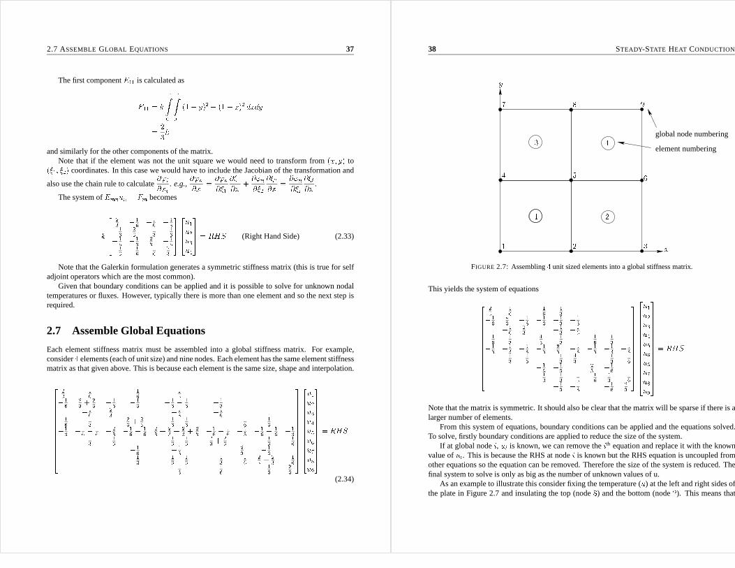
2.7 Assemble Global Equations
Each element stiffness matrix must be assembled into a global stiffness matrix. For example,consider4 elements (each of unit size) and nine nodes. Each element hasthe same element stiffnessmatrix as that given above. This is because each element is the same size, shape and interpolation.26666666666664
23 �16 �16 �13�16 23 + 23 �16 �13 �16 � 16 �13�16 23 �13 �16�16 �13 23 + 23 �16 � 16 �16 �13�13 �16 � 16 �23 �16 � 16 23 + 23 + 23 + 23 �16 � 16 �13 �16 � 16 �13�13 �16 �16 � 16 23 + 23 �13 �16�16 �13 23 �16�13 �16 � 16 �13 �16 23 + 23 �16�13 �16 �16 233777777777777526666666666664u1u2u3u4u5u6u7u8u937777777777775 = RHS
(2.34)
38 STEADY-STATE HEAT CONDUCTION
3 47 81
y
29
3 xelement numbering
global node numbering
2654
1FIGURE 2.7: Assembling4 unit sized elements into a global stiffness matrix.
This yields the system of equations2666666666666423 �16 �16 �13�16 43 �16 �13 �13 �13�16 23 �13 �16�16 �13 43 �13 �16 �13�13 �13 �13 �13 83 �13 �13 �13 �13�13 �16 �13 43 �13 �16�16 �13 23 �16�13 �13 �13 �16 43 �16�13 �16 �16 23377777777777752666666666666664u1u2u3u4u5u6u6u7u8u93777777777777775 = RHS
Note that the matrix is symmetric. It should also be clear that the matrix will be sparse if there is alarger number of elements.
From this system of equations, boundary conditions can be applied and the equations solved.To solve, firstly boundary conditions are applied to reduce the size of the system.
If at global nodei, ui is known, we can remove theith equation and replace it with the knownvalue ofui. This is because the RHS at nodei is known but the RHS equation is uncoupled fromother equations so the equation can be removed. Therefore the size of the system is reduced. Thefinal system to solve is only as big as the number of unknown values of u.
As an example to illustrate this consider fixing the temperature (u) at the left and right sides ofthe plate in Figure 2.7 and insulating the top (node8) and the bottom (node2). This means that

2.8 GAUSSIAN QUADRATURE 39
there are only3 unknown values of u at nodes (2,5 and 8), therefore there is a3�3 matrix to solve.The RHS is known at these three nodes (see below). We can then solve the3� 3 matrix and thenmultiply out the original matrix to find the unknown RHS values.
The RHS is0 at nodes2 and8 because it is insulated. To find out what the RHS is at node5
we need to examine the RHS expression
Z� @u@n! d� = 0 at node5. This is zero as flux is always0 at internal nodes. This can be explained in two ways.1 2
nn
FIGURE 2.8: “Cancelling” of flux in internal nodes.
Correct way: � does not pass through node5 and each basis function that is not zero at5 is zeroon�
Other way:
@u@n is opposite in neighbouring elements so it cancels (see Figure 2.8).
2.8 Gaussian Quadrature
The element integrals arising from two- or three-dimensional problems can seldom be evaluated an-alytically. Numerical integration orquadratureis therefore required and the most efficient schemefor integrating the expressions that arise in the finite element method is Gauss-Legendre quadra-ture.
Consider first the problem of integratingf (�) between the limits0 and 1 by the sum ofweighted samples off (�) taken at points�1; �2; : : : ; �I (see Figure 2.3):1Z0 f (�) d� = IXi=1 Wif (�i) + EHereWi are the weights associated with sample points�i - calledGauss points- andE is theerror in the approximation of the integral. We now choose theGauss points and weights to exactlyintegrate a polynomial of degree2I � 1 (since a general polynomial of degree2I � 1 has2Iarbitrary coefficients and there are2I unknown Gauss points and weights).
For example, withI = 2 we can exactly integrate a polynomial of degree 3:
40 STEADY-STATE HEAT CONDUCTION
��1 �20 1�I
f (�). . . .
. . . .FIGURE 2.9: Gaussian quadrature.f (�) is sampled atI Gauss points�1; �2 : : : �I :
Let
1Z0 f (�) d� =W1f (�1) +W2f (�2)
and choosef (�) = a+ b� + c�2 + d�3. Then1Z0 f (�) d� = a 1Z0 d� + b 1Z0 � d� + c 1Z0 �2 d� + d 1Z0 �3 d� (2.35)
Sincea, b, c andd are arbitrary coefficients, each integral on the RHS of 2.35 must be integratedexactly. Thus, 1Z0 d� = 1 =W1:1 +W2:1 (2.36)1Z0 � d� = 12 =W1:�1 +W2:�2 (2.37)1Z0 �2 d� = 13 =W1:�21 +W2:�22 (2.38)1Z0 �3 d� = 14 =W1:�31 +W2:�32 (2.39)
These four equations yield the solution for the two Gauss points and weights as follows:

2.8 GAUSSIAN QUADRATURE 41
From symmetry and Equation (2.36),W1 =W2 = 12 :
Then, from (2.37), �2 = 1� �1
and, substituting in (2.38), �21 + (1� �1)2 = 232�21 � 2�1 + 13 = 0;
giving �1 = 12 � 12p3 :
Equation (2.39) is satisfied identically. Thus, the two Gauss points are given by�1 = 12 � 12p3 ;�2 = 12 + 12p3 ;W1 =W2 = 12 (2.40)
A similar calculation for a5th degree polynomial using three Gauss points gives�1 = 12 � 12r35 ; W1 = 518�2 = 12 ; W2 = 49 (2.41)�3 = 12 + 12r35 ; W3 = 518For two- or three-dimensional Gaussian quadrature the Gauss point positions are simply the valuesgiven above along each�i-coordinate with the weights scaled to sum to1 e.g., for 2x2 Gauss
quadrature the4 weights are all
14 . The number of Gauss points chosen for each�i-direction is
governed by the complexity of the integrand in the element integral (2.8). In general two- and three-
dimensional problems the integral is not polynomial (owingto the@�i@xj terms which come from the
42 STEADY-STATE HEAT CONDUCTION
inverse of the matrix
�@xi@�j �) and no attempt is made to achieve exact integration. The quadrature
error must be balanced against the discretization error. For example, if the two-dimensional basisis cubic in the�1-direction and linear in the�2-direction, three Gauss points would be used in the�1-direction and two in the�2-direction.
2.9 CMISS Examples
1. To solve for the steady state temperature distribution inside a plate run CMISS example311
2. To solve for the steady state temperature distribution inside an annulus run CMISS example3123. To investigate the convergence of the steady state temperature distribution with mesh refine-
ment run CMISS examples3141, 3142, 3143 and3144.

Chapter 3
The Boundary Element Method
3.1 Introduction
Having developed the basic ideas behind the finite element method, we now develop the basic ideasof the boundary element method. There are several key differences between these two methods,one of which involves the choice of weighting function (recall the Galerkin finite element methodused as a weighting function one of the basis functions used to approximate the solution variable).Before launching into the boundary element method we must briefly develop some ideas that arecentral to the weighting function used in the boundary element method.
3.2 The Dirac-Delta Function and Fundamental Solutions
Before one applies the boundary element method to a particular problem one must obtain afunda-mental solution(which is similar to the idea of a particular solution in ordinary differential equa-tions and is the weighting function). Fundamental solutions are tied to the Dirac1 Delta functionand we deal with both here.
3.2.1 Dirac-Delta function
What we do here is very non-rigorous. To gain an intuitive feel for this unusual function, considerthe following sequence of force distributions applied to a large plate as shown in Figure 3.1wn (x) = �n2 jxj < 1n0 jxj > 1n
1Paul A.M. Dirac (1902-1994) was awarded the Nobel Prize (with Erwin Schrodinger) in 1933 for his work inquantum mechanics. Dirac introduced the idea of the “Dirac Delta” intuitively, as we will do here, around 1926-27.It was rigorously defined as a so-called generalised function by Schwartz in 1950-51, and strictly speaking we shouldtalk about the “Dirac Delta Distribution”.
44 THE BOUNDARY ELEMENT METHOD
Each has the property that1Z�1 wn (x) dx = 1 (i.e., the total force applied is unity)
but asn increases the area of force application decreases and the force/unit area increases.
12 14 131
12 1232 w4w3 w2 w1
FIGURE 3.1: Illustrations of unit force distributionswn.
As n gets larger we can easily see that the area of application of the force becomes smallerand smaller, the magnitude of the force increases but the total force applied remains unity. If weimagine lettingn ! 1 we obtain an idealised “point” force of unit strength, giventhe symbol� (x), acting atx = 0. Thus, in a nonrigorous sense we have� (x) = limn!1wn (x) the Dirac Delta“function”.
This is not a function that we are used to dealing with becausewe have� (x) = 0 if x 6= 0
and “� (0) = 1” i.e., the “function” is zero everywhere except at the origin, where it is infinite.
However, we have
1Z�1 � (x) dx = 1 since each
1Z�1 wn (x) dx = 1.
The Dirac delta “function” is not a function in the usual sense, and it is more correctly referredto as the Dirac delta distribution. It also has the property that for any continuous functionh (x)1Z�1 � (x) h (x) dx = h (0) (3.1)
3.2 THE DIRAC-DELTA FUNCTION AND FUNDAMENTAL SOLUTIONS 45
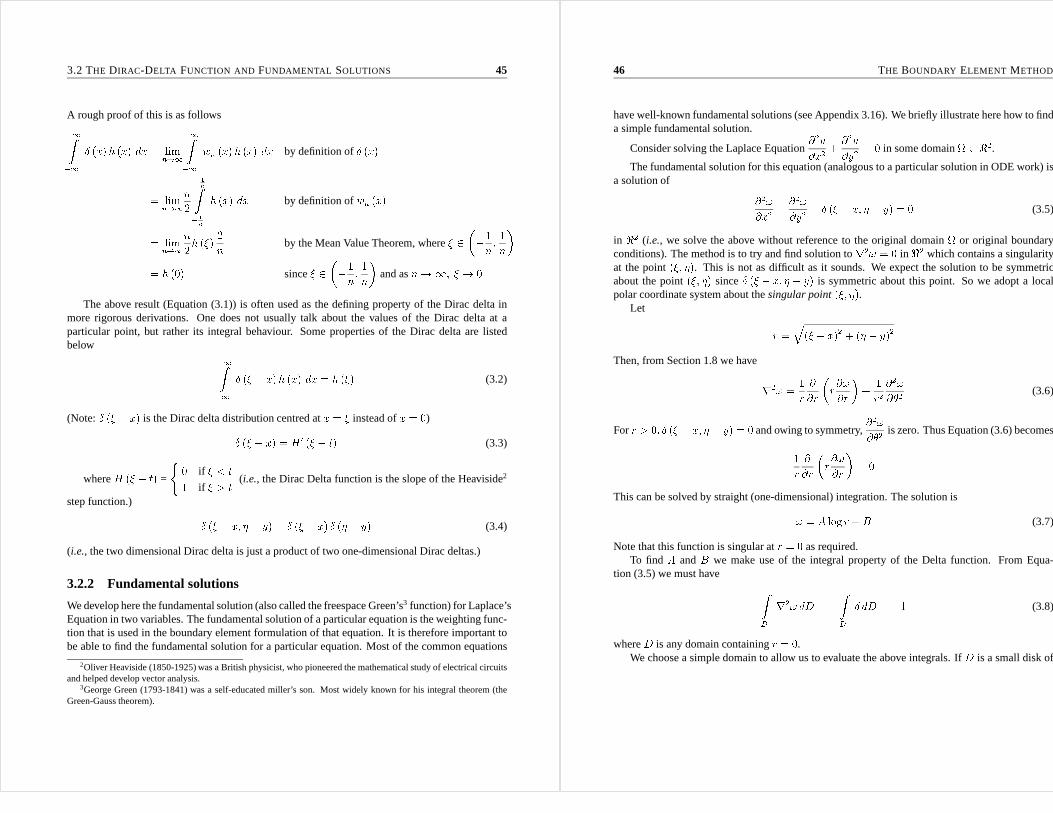
A rough proof of this is as follows1Z�1 � (x) h (x) dx = limn!1 1Z�1 wn (x) h (x) dx by definition of� (x)= limn!1n2 1nZ� 1n h (x) dx by definition ofwn (x)= limn!1n2h (�) 2n by the Mean Value Theorem, where� 2 �� 1n; 1n�= h (0) since� 2 �� 1n; 1n� and asn!1; � ! 0
The above result (Equation (3.1)) is often used as the defining property of the Dirac delta inmore rigorous derivations. One does not usually talk about the values of the Dirac delta at aparticular point, but rather its integral behaviour. Some properties of the Dirac delta are listedbelow 1Z�1 � (� � x) h (x) dx = h (�) (3.2)
(Note: � (� � x) is the Dirac delta distribution centred atx = � instead ofx = 0)� (� � x) = H 0 (� � t) (3.3)
whereH (� � t) =
( 0 if � < t1 if � > t (i.e., the Dirac Delta function is the slope of the Heaviside2
step function.) � (� � x; � � y) = � (� � x) � (� � y) (3.4)
(i.e., the two dimensional Dirac delta is just a product of two one-dimensional Dirac deltas.)
3.2.2 Fundamental solutions
We develop here the fundamental solution (also called the freespace Green’s3 function) for Laplace’sEquation in two variables. The fundamental solution of a particular equation is the weighting func-tion that is used in the boundary element formulation of thatequation. It is therefore important tobe able to find the fundamental solution for a particular equation. Most of the common equations
2Oliver Heaviside (1850-1925) was a British physicist, who pioneered the mathematical study of electrical circuitsand helped develop vector analysis.
3George Green (1793-1841) was a self-educated miller’s son.Most widely known for his integral theorem (theGreen-Gauss theorem).
46 THE BOUNDARY ELEMENT METHOD
have well-known fundamental solutions (see Appendix 3.16). We briefly illustrate here how to finda simple fundamental solution.
Consider solving the Laplace Equation
@2u@x2 + @2u@y2 = 0 in some domain 2 <2.The fundamental solution for this equation (analogous to a particular solution in ODE work) is
a solution of @2!@x2 + @2!@y2 + � (� � x; � � y) = 0 (3.5)
in <2 (i.e., we solve the above without reference to the original domain or original boundaryconditions). The method is to try and find solution tor2! = 0 in <2 which contains a singularityat the point(�; �). This is not as difficult as it sounds. We expect the solution to be symmetricabout the point(�; �) since� (� � x; � � y) is symmetric about this point. So we adopt a localpolar coordinate system about thesingular point(�; �).
Let r =q(� � x)2 + (� � y)2
Then, from Section 1.8 we haver2! = 1r @@r �r@!@r �+ 1r2 @2!@�2 (3.6)
Forr > 0; � (� � x; � � y) = 0 and owing to symmetry,
@2!@�2 is zero. Thus Equation (3.6) becomes1r @@r �r@!@r � = 0
This can be solved by straight (one-dimensional) integration. The solution is! = A log r +B (3.7)
Note that this function is singular atr = 0 as required.To find A andB we make use of the integral property of the Delta function. From Equa-
tion (3.5) we must have ZD r2! dD = � ZD � dD = �1 (3.8)
whereD is any domain containingr = 0.We choose a simple domain to allow us to evaluate the above integrals. IfD is a small disk of

3.2 THE DIRAC-DELTA FUNCTION AND FUNDAMENTAL SOLUTIONS 47
"(�; �)
x
yD
FIGURE 3.2: Domain used to evaluate fundamental solution coefficients.
radius" > 0 centred atr = 0 (Figure 3.2) then from the Green-Gauss theoremZD r2! dD = Z@D @!@n dS @D is the surface of the diskD= Z@D @!@r dS sinceD is a disk centred atr = 0 son andr are in the same direction= A" 2�" from Equation (3.7), and the fact thatD is a disc of radius"= 2�A
Therefore, from Equation (3.8) A = � 12� :
So we have ! = � 12� log r +BB remains arbitrary but usually put equal to zero, so that the fundamental solution for the two-dimensional Laplace Equation is! = � 12� log r �= 12� log 1r� (3.9)
48 THE BOUNDARY ELEMENT METHOD
wherer =q(� � x)2 + (� � y)2 (singular at the point(�; �)).The fundamental solution for the three-dimensional Laplace Equation can be found by a similar
technique. The result is ! = 14�rwherer is now a distance measured in three-dimensions.
3.3 The Two-Dimensional Boundary Element Method
We are now at a point where we can develop the boundary elementmethod for the solution ofr2u = 0 in a two-dimensional domain. The basic steps are in fact quite similar to those used forthe finite element method (refer Section 2.1). We firstly mustform an integral equation from theLaplace Equation by using a weighted integral equation and then use the Green-Gauss theorem.From Section 2.4 we have seen that0 = Z r2u:! d = Z@ @u@n! d�� Z ru:r! d (3.10)
This was the starting point for the finite element method. To derive the starting equation forthe boundary element method we use the Green-Gauss theorem again on the second integral. Thisgives 0 = Z@ @u@n! d�� Z ru:r! d= Z@ @u@n! d�� Z@ u@!@n d� + Z ur2! d (3.11)
For the Galerkin FEM we chose!, the weighting function, to be'm, one of the basis functionsused to approximateu. For the boundary element method we choose! to be the fundamentalsolution of Laplace’s Equation derived in the previous section i.e.,! = � 12� log r
wherer =q(� � x)2 + (� � y)2 (singular at the point(�; �) 2 ).Then from Equation (3.11), using the property of the Dirac deltaZ ur2! d = � Z u� (� � x; � � y) d = �u (�; �) (�; �) 2 (3.12)
i.e., the domain integral has been replaced by a point value.

3.3 THE TWO-DIMENSIONAL BOUNDARY ELEMENT METHOD 49
Thus Equation (3.11) becomesu (�; �) + Z@ u@!@n d� = Z@ @u@n! d� (�; �) 2 (3.13)
This equation contains only boundary integrals (and no domain integrals as in Finite Elements)and is referred to as a boundary integral equation. It relates the value ofu at some point inside
the solution domain to integral expressions involvingu and
@u@n over the boundary of the solution
domain. Rather than having an expression relating the valueof u at some point inside the domainto boundary integrals, a more useful expression would be onerelating the value ofu at some pointon the boundaryto boundary integrals. We derive such an expression below.
The previous equation (Equation (3.13)) holds if(�; �) 2 (i.e., the singularity of Dirac Deltafunction is inside the domain). If(�; �) is outside thenZ ur2! d = � Z u� (� � x; � � y) d = 0
since the integrand of the second integral is zero at every point except(�; �) and this point isoutside the region of integration. The case which needs special consideration is when the singularpoint (�; �) is on the boundary of the domain. This case also happens to be the most importantfor numerical work as we shall see. The integral expression we will ultimately obtain is simply
Equation (3.13) withu (�; �) replaced by
12u (�; �). We can see this in a non-rigorous way as
follows. When(�; �) was inside the domain, we integrated around the entire singularity of theDirac Delta to getu (�; �) in Equation (3.13). When(�; �) is on the boundary we only have half ofthe singularity contained inside the domain, so we integrate around one-half of the singularity to
get
12u (�; �). Rigorous details of where this coefficient
12 comes from are given below.
Let P denote the point(�; �) 2 . In order to be able to evaluate
Z ur2! d in this case we
enlarge to include a disk of radius" aboutP (Figure 3.3). We call this enlarged region0 andlet �0 = ��" [ �".
Now, sinceP is inside the enlarged region0, Equation (3.13) holds for this enlarged domaini.e., u (P ) + Z��"[�" u@!@n d� = Z��"[�" @u@n! d� (3.14)
We must now investigate this equation aslim"#0 . There are4 integrals to consider, and we look ateach of these in turn.
50 THE BOUNDARY ELEMENT METHOD
0 �""P ��"
FIGURE 3.3: Illustration of enlarged domain when singular point ison the boundary.
Firstly considerZ�" u@!@n d� = Z�" u @@n �� 12� log r� d� by definition of!= Z�" u @@r �� 12� log r� d� since
@@n � @@r on�"= � 12� Z�" ur d�= � 12� 1" Z�" u d� sincer = " on�"! � 12� 1"u (P )�"
by the mean value theorem for a surface with a unique tangent at P .Thus lim"#0 Z�" u@!@n d� = lim"#0 �� 12� u (P )" �"� = �u (P )2 (3.15)
By a similar process we obtainlim"#0 Z�" !@u@n d� = lim"#0 �� 12� @u@n (P )�" log "� = 0 (3.16)
sincelim" log "#0 aslim"#0 .

3.3 THE TWO-DIMENSIONAL BOUNDARY ELEMENT METHOD 51
It only remains to consider the integrand over��". For “nice” integrals (which includes theintegrals we are dealing with here) we havelim"#0 0@ Z��" (nice integrand)d�1A = Z� (nice integrand)d�
since��" ! � aslim"#0 .Note: If the integrand is too badly behaved we cannot always replace��" by� in the limit and
one must deal with Cauchy Principal Values. (refer Section 5.8)Thus we have lim"!00@ Z��" @u@n! d�1A = Z� @u@n! d� (3.17)lim"!00@ Z��" @!@nu d�1A = Z� @!@nu d� (3.18)
Combining Equations (3.14)–(3.18) we getu (P ) + Z� u@!@n d� = 12u (P ) + Z� @u@n! d�
or 12u (P ) + Z� u@!@n d� = Z� @u@n! d�
whereP = (�; �) 2 @ (i.e.,singular point is on the boundary of the region).Note: The above is true if the pointP is at a smooth point (i.e.,a point with a unique tangent) on
the boundary of. If P happens to lie at some nonsmooth point e.g. a corner, then thecoefficient12 is replaced by
�2� where� is the internal angle atP (Figure 3.4).P �
FIGURE 3.4: Illustration of internal angle�.
52 THE BOUNDARY ELEMENT METHOD
Thus we get the boundary integral equation.c (P )u (P ) + Z� u@!@n d� = Z� @u@n! d� (3.19)
where ! = � 12� log rr =q(� � x)2 + (� � y)2c (P ) = 8><>: 1 if P 2 12 if P 2 � and� smooth atP
internal angle2� if P 2 � and� not smooth atP
For three-dimensional problems, the boundary integral equation expression above is the same,with ! = 14�rr =q(� � x)2 + (� � y)2 + ( � z)2c (P ) = 8><>: 1 if P 2 12 if P 2 � and� smooth atP
inner solid angle4� if P 2 � and� not smooth atP
Equation (3.19) involves only the surface distributions ofu and
@u@n and the value ofu at a
point P . Once the surface distributions ofu and
@u@n are known, the value ofu at any pointP
inside can be found since all surface integrals in Equation (3.19) are then known. The procedure
is thus to use Equation (3.19) to find the surface distributions ofu and
@u@n and then (if required)
use Equation (3.19) to find the solution at any pointP 2 . Thus we solve for the boundary datafirst, and find the volume data as a separate step.
Since Equation (3.19) only involves surface integrals, as opposed to volume integrals in a finiteelement formulation, the overall size of the problem has been reduced by one dimension (fromvolumes to surfaces). This can result in huge savings for problems with large volume to surfaceratios (i.e.,problems with large domains). Also the effort required to produce a volume mesh of acomplex three-dimensional object is far greater than that required to produce a mesh of the surface.Thus the boundary element method offers some distinct advantages over the finite element methodin certain situations. It also has some disadvantages when compared to the finite element methodand these will be discussed in Section 3.6. We now turn our attention to solving the boundaryintegral equation given in Equation (3.19).

3.4 NUMERICAL SOLUTION PROCEDURES FOR THEBOUNDARY INTEGRAL EQUATION 53
3.4 Numerical Solution Procedures for the Boundary IntegralEquation
The first step is to discretise the surface� into some set of elements (hence the name boundaryelements). � = N[j=1�j (3.20)
(b)(a)
FIGURE 3.5: Schematic illustration of a boundary element mesh (a) and a finite element mesh (b).
Then Equation (3.19) becomesc (P )u (P ) + NXj=1 Z�j u@!@n d� = NXj=1 Z�j @u@n! d� (3.21)
Over each element�j we introduce standard (finite element) basis functionsuj =X� '�uj� and qj � @uj@n =X� '�qj� (3.22)
whereuj; qj are values ofu andq on element�j anduj�; qj� are values ofu andq at node� onelement�j.
These basis functions foru andq can be any of the standard one-dimensional finite elementbasis functions (although we are dealing with a two-dimensional problem, we only have to inter-polate the functions over a one-dimensional element). In general the basis functions used foru andq do not have to be the same (typically they are) and these basisfunctions can even be different tothe basis functions used for the geometry, but are generallytaken to be the same (this is termed anisoparametric formulation).
54 THE BOUNDARY ELEMENT METHOD
This gives c (P )u (P ) + NXj=1X� uj� Z�j '�@!@n d� = NXj=1X� qj� Z�j '�! d� (3.23)
This equation holds for any pointP on the surface�. We now generate one equation per node byputting the pointP to be at each node in turn. IfP is at nodei, say, then we haveciui + NXj=1X� uj� Z�j '�@!i@n d� = NXj=1X� qj� Z�j '�!i d� (3.24)
where!i is the fundamental solution with the singularity at nodei (recall! is� 12� log r , wherer is the distance from the singularity point). We can write Equation (3.24) in a more abbreviatedform as ciui + NXj=1X� uj�a�ij = NXj=1X� qj�b�ij (3.25)
where a�ij = Z�j '�@!i@n d� and b�ij = Z�j '�!i d� (3.26)
Equation (3.25) is for nodei and if we haveL nodes, then we can generateL equations.We can assemble these equations into the matrix systemAu = Bq (3.27)
(compare to the global finite element equationsKu = f ) where the vectorsu andq are the vectorsof nodal values ofu andq. Note that theij th component of theA matrix in general isnot a�ij andsimilarly forB.
At each node, we must specify either a value ofu or q (or some combination of these) to have awell-defined problem. We therefore haveL equations (the number of nodes) and haveL unknownsto find. We need to rearrange the above system of equations to getCx = f (3.28)
wherex is the vector of unknowns. This can be solved using standard linear equation solvers,although specialist solvers are required if the problem is large (refer[todo : Section ???]).
The matricesA andB (and henceC) are fully populated and not symmetric (compare to thefinite element formulation where the global stiffness matrix K is sparse and symmetric). Thesize of theA andB matrices are dependent on the number of surface nodes, whilethe matrixK is dependent on the number of finite element nodes (which include nodes in the domain). As

3.5 NUMERICAL EVALUATION OF COEFFICIENT INTEGRALS 55
mentioned earlier, it depends on the surface to volume ratioas to which method will generate thesmallest and quickest solution.
The use of the fundamental solution as a weight function ensures that theA andB matricesare generally well conditioned (see Section 3.5 for more on this). In fact theAmatrix is diagonallydominant (at least for Laplace’s equation). The matrixC is therefore also well conditioned andEquation (3.28) can be solved reasonably easily.
The vectorx contains the unknown values ofu andq on the boundary. Once this has beenfound, all boundary values ofu andq are known. If a solution is then required at a point inside thedomain, then we can use Equation (3.25) with the singular pointP located at the required solutionpoint i.e., u (P ) = NXj=1X� qj�b�Pj � NXj=1X� uj�a�Pj (3.29)
The right hand side of Equation (3.29) contains no unknowns and only involves evaluating thesurface integrals using the fundamental solution with the singular point located atP .
3.5 Numerical Evaluation of Coefficient Integrals
We consider in detail here how one evaluates thea�ij andb�ij integrals for two-dimensional problems.These integrals typically must be evaluated numerically, and require far more work and effort thanthe analogous finite element integrals.
Recall that a�ij = Z�j '�@!i@n d� and b�ij = Z�j '�!i d�
where !i = � 12� log riri = distance measured from nodeiIn terms of a local� coordinate we haveb�ij = 1Z0 '� (�)!i (�) jJ (�)j d� (3.30)a�ij = Z�j '� (�) @!i (�)@n jJ (�)j d� = 1Z0 '� (�) @!i@ri (�) dridn jJ (�)j d� (3.31)
56 THE BOUNDARY ELEMENT METHOD
The JacobianJ (�) can be found byJ (�) = d�d� = dsd� =s�dxd��2 + �dyd��2(3.32)
wheres represents the arclength and
dxd� and
dyd� can be found by straight differentiation of the
interpolation expression forx (�) andy (�).The fundamental solution is!i = � 12� log (ri (�))ri (�) =q(x (�)� xi)2 + (y (�)� yi)2
where(xi; yi) are the coordinates of nodei.To find
dridn we note that dridn = rri � ^n (3.33)
where^n is a unit outward normal vector. To find a unit normal vector, we simply rotate the tangent
vector (given by(x0 (�) ; y0 (�)) ) by
�2 in the appropriate direction and then normalise.
Thus every expression in the integrands of thea�ij andb�ij integrals can be found at any value of�, and the integrals can therefore be evaluated numerically using some suitable quadrature schemes.If node i is well removed from element�j then standard Gaussian quadrature can be used to
evaluate these integrals. However, if nodei is in �j (or close to it) we see thatri approaches 0and the fundamental solution!i tends to1. The integral still exists, but the integrand becomessingular. In such cases special care must be taken - either byusing special quadrature schemes,large numbers of Gauss points or other special treatment.
The integrals for which nodei lies in element�j are in general the largest in magnitude andlead to the diagonally dominant matrix equation. It is therefore important to ensure that theseintegrals are calculated as accurately as possible since these terms will have most influence on thesolution. This is one of the disadvantages of the BEM - the fact that singular integrands must beaccurately integrated.
A relatively straightforward way to evaluate all the integrals is simply to use Gaussian quadra-ture with varying number of quadrature points, depending onhow close or far the singular point isfrom the current element. This is not very elegant or efficient, but has the benefit that it is relativelyeasy to implement. For the case when nodei is contained in the current element one can use specialquadrature schemes which are designed to integrate log-type functions. These are to be preferredwhen one is dealing with Laplace’s equation. However, thesespecial log-type schemes cannot beso readily used on other types of fundamental solution so fora general purpose implementation,Gaussian quadrature is still the norm. It is possible to incorporate adaptive integration schemesthat keep adding more quadrature points until some error estimate is small enough, or also to sub-divide the current element into two or more smaller elementsand evaluate the integral over each

3.6 THE THREE-DIMENSIONAL BOUNDARY ELEMENT METHOD 57
(a)
ri
nodei�j ri �jnodei
(b)
FIGURE 3.6: Illustration of the decrease inri as nodei approaches element�j.subelement. It is also possible to evaluate the “worst” integrals by using simple solutions to thegoverning equation, and this technique is the norm for elasticity problems (Section 5.8). Detailson each of these methods is given in Section 3.8. It should be noted that research still continues inan attempt to find more efficient ways of evaluating the boundary element integrals.
3.6 The Three-Dimensional Boundary Element Method
The three-dimensional boundary element method is very similar to the two-dimensional bound-ary element method discussed above. As noted above, the three-dimensional boundary integralequation is the same as the two-dimensional equation (3.19), with ! andc (P ) being defined asin Section 3.3. The numerical solution procedure also parallels that given in Section 3.4, and theexpressions given fora�ij andb�ij apply equally well to the three-dimensional case. The only realdifference between the two procedures is how to numericallyevaluate the terms in each integrandof these coefficient integrals.
As in Section 3.5 we illustrate how to evaluate each of the terms in the integrand ofa�ij andb�ij.
58 THE BOUNDARY ELEMENT METHOD
The relevant expressions area�ij = Z�j '�@!i@n d�= 1Z0 1Z0 '� (�1; �2) @!i@ri (�1; �2) dridn jJ (�1; �2)j d�1 d�2 (3.34)b�ij = Z�j '�!i d�= 1Z0 1Z0 '� (�1; �2)!i (�1; �2) jJ (�1; �2)j d�1 d�2 (3.35)
The fundamental solution is!i (�1; �2) = 14�ri (�1; �2)whereri (�1; �2) =q(x (�1; �2)� xi)2 + (y (�1; �2)� yi)2 + (z (�1; �2)� zi)2
where(xi; yi; zi) are the coordinates of nodei. As before we use
dridn = rri � ^n to find
dridn .
The unit outward normal^n is found by normalising the cross product of the two tangent vectorst1 = � @x@�1 ; @y@�1 ; @z@�1� and t2 = � @x@�2 ; @y@�2 ; @z@�2� (it relies on the user of any BEM code to
ensure that the elements have been defined with a consistent set of element coordinates�1 and�2).The JacobianJ (�1; �2) is given bykt1 � t2k (wheret1 andt2 are the two tangent vectors).
Note that this is different for the determinant in a two-dimensional finite element code - in thatcase we are dealing with a two-dimensional surface in two-dimensional space, whereas here wehave a (possibly curved) two-dimensional surface in three-dimensional space.
The integrals are evaluated numerically using some suitable quadrature schemes (see Sec-tion 3.8) (typically a Gauss-type scheme in both the�1 and�2 directions).
3.7 A Comparison of the FE and BE Methods
We comment here on some of the major differences between the two methods. Depending on theapplication some of these differences can either be considered as advantageous or disadvantageousto a particular scheme.
1. FEM : An entire domain mesh is required.BEM : A mesh of the boundary only is required.Comment: Because of the reduction in size of the mesh, one often hearsof people sayingthat the problem size has been reduced by one dimension. Thisis one of the major pluses of

3.7 A COMPARISON OF THEFE AND BE METHODS 59
the BEM - construction of meshes for complicated objects, particularly in 3D, is a very timeconsuming exercise.
2. FEM : Entire domain solution is calculated as part of the solution.BEM : Solution on the boundary is calculated first, and then the solution at domain points (ifrequired) are found as a separate step.Comment: There are many problems where the details of interest occuron the boundary, orare localised to a particular part of the domain, and hence anentire domain solution is notrequired.
3. FEM : Reactions on the boundary typically less accurate than thedependent variables.BEM : Bothu andq of the same accuracy.
4. FEM : Differential Equation is being approximated.BEM : Only boundary conditions are being approximated.Comment: The use of the Green-Gauss theorem and a fundamental solution in the formu-lation means that the BEM involves no approximations of the differential Equation in thedomain - only in its approximations of the boundary conditions.
5. FEM : Sparse symmetric matrix generated.BEM : Fully populated nonsymmetric matrices generated.Comment: The matrices are generally of different sizes due to the differences in size ofthe domain mesh compared to the surface mesh. There are problems where either methodcan give rise to the smaller system and quickest solution - itdepends partly on the volumeto surface ratio. For problems involving infinite or semi-infinite domains, BEM is to befavoured.
6. FEM : Element integrals easy to evaluate.BEM : Integrals are more difficult to evaluate, and some contain integrands that becomesingular.Comment: BEM integrals are far harder to evaluate. Also the integrals that are the mostdifficult (those containing singular integrands) have a significant effect on the accuracy ofthe solution, so these integrals need to be evaluated accurately.
7. FEM : Widely applicable. Handles nonlinear problems well.BEM : Cannot even handle all linear problems.Comment: A fundamental solution must be found (or at least an approximate one) before theBEM can be applied. There are many linear problems (e.g.,virtually any nonhomogeneousequation) for which fundamental solutions are not known. There are certain areas in whichthe BEM is clearly superior, but it can be rather restrictivein its applicability.
8. FEM : Relatively easy to implement.BEM : Much more difficult to implement.Comment: The need to evaluate integrals involving singular integrands makes the BEM atleast an order of magnitude more difficult to implement than acorresponding finite elementprocedure.
60 THE BOUNDARY ELEMENT METHOD
3.8 More on Numerical Integration
The BEM involves integrals whose integrands in generally become singular when the source pointis contained in the element of integration. If one uses constant or linear interpolation for thegeometry and dependent variable, then it is possible to obtain analytic expressions to most (if notall) of the integrals that will appear in the BEM (at least fortwo-dimensional problems). Theexpressions can become quite lengthy to write down and evaluate, but benefit from the fact thatthey will be exact. However, when one begins to use general curved elements and/or solve three-dimensional problems then the integrals will not be available as analytic expressions. The basictool for evaluation of these integrals is quadrature. As discussed in Section 2.8 a one-dimensionalintegral is approximated by a sum in which the integrand is evaluated at certain discrete points orabscissa 1Z0 f (�) d� � NXi=1 f (�i)wi
wherewi are the weights and�i are the abscissa.The weights and abscissa for the Gaussian quadrature schemeof orderN are chosen so that the
above expression will exactly integrate any polynomial of degree2N�1 or less. For the numericalevaluation of two or three-dimensional integrals, a Gaussian scheme can be used of each variableof integration if the region of integration is rectangular.This is generally not the optimal choicefor the weights and abscissae but it allows easy extension tohigher order integration.
3.8.1 Logarithmic quadrature and other special schemes
Low order Gaussian schemes are generally sufficient for all FEM integrals, but that is not thecase for BEM. For a two-dimensional BEM solution of Laplace’s equation, integrals of the form1Z0 log (�) f (�) d� will be required. It is relatively common to use logarithmicschemes for this.
These are obtained by approximating the integral as1Z0 log (�) f (�) d� � NXi=1 f (�i)wi
i.e., the log function has been factored out.In the same way as Gaussian quadrature schemes were developed in Section 2.8, log quadrature
schemes can be developed which will exactly integrate polynomial functionsf (�). Tables of theseare given below
It is possible to develop similar quadrature schemes for usein the BEM solution of other PDEs,which use different fundamental solutions to the log function. The problem with this approach isthe lack of generality - each new equation to be used requiresits own special quadrature scheme.

3.9 THE BOUNDARY ELEMENT METHOD APPLIED TO OTHERELLIPTIC PDES 61
Abscissas =ri Weight Factors =win �i �wi n �i �wi n �i �wi
2 0.112009 0.718539 3 0.063891 0.513405 4 0.041448 0.3834640.602277 0.281461 0.368997 0.391980 0.245275 0.386875
0.766880 0.094615 0.556165 0.1904350.848982 0.039225
TABLE 3.1: Abscissas and weight factors for Gaussian integrationfor integrands with alogarithmic singularity.
3.8.2 Special solutions
Another approach, particularly useful if Cauchy principalvalues are to be found (see Section 5.8) isto use special solutions of the governing equation to find oneor more of the more difficult integrals.
For exampleu = x is a solution to Laplaces’ equation (assuming the boundary conditionsare set correctly). Thus if one sets bothu andq in Equation (3.27) at every node according tothe solutionu = x, one can then use this to solve for some entry in either theA or B matrix(typically the diagonal entry since this is the most important and difficult to find). Further solutionsto Laplaces equation (e.g.,u = x2 � y2) can be used to find the other matrix entries (or just usedto check the accuracy of the matrices).
3.9 The Boundary Element Method Applied to other EllipticPDEs
Helmholtz, modified Helmholtz (CMISS example) Poisson Equation (domain integral and MRM,DRM, Monte-carlo integration.
3.10 Solution of Matrix Equations
The standard BEM approach results in a system of equations ofthe formCx = f (refer (3.28)).As mentioned above the matrixC is generally well conditioned, fully populated and nonsymmet-ric. For small problems, direct solution methods, based on LU factorisations, can be used. As theproblem size increases, the time taken for the matrix solution begins to dominate the matrix assem-bly stage. This usually occurs when there is between500 and1000 degrees of freedom, although itis very dependent on the implementation of the BE method. Thecurrent technique of favour in theBE community for solution of large BEM matrix equations is a preconditioned Conjugate Gradientsolver. Preconditioners are generally problem dependent -what works well for one problem maynot be so good for another problem. The conjugate gradient technique is generally regarded as asolution technique for (sparse) symmetric matrix equations.
62 THE BOUNDARY ELEMENT METHOD
B�I
f�f�B
FIGURE 3.7: Coupled finite element/boundary element solution domain.
3.11 Coupling the FE and BE techniques
There are undoubtably situations which favour FEM over BEM and vice versa. Often one problemcan give rise to a model favouring one method in one region andthe other method in anotherregion,e.g., in a detailed analysis of stresses around a foundation one needs FEM close to thefoundation to handle nonlinearities, but to handle the semi-infinite domain (well removed from thefoundation), BEM is better. There has been a lot of research on coupling FE and BE procedures -we will only talk about the basic ideas and use Laplace’s Equation to illustrate this. There are atleast two possible methods.
1. Treat the BEM region as a finite element and combine with FEM
2. Treat the FEM region as an equivalent boundary element andcombine with BEM
Note that these are essentially equivalent - the use of one orthe other depends on the problem,in the sense of which part is more dominant FEM or BEM)
Consider the region shown in Figure 3.7, wheref = FEM regionB = BEM region�f = FEM boundary�B = BEM boundary�I = interface boundary
The BEM matrices forB can be written asAu = Bq (3.36)
whereu is a vector of the nodal values ofu andq is a vector of the nodal values of
@u@n
The FEM matrices forF can be written asKu = f (3.37)

3.11 COUPLING THE FE AND BE TECHNIQUES 63
whereK is the stiffness matrix andf is the load vector.To apply method1 (i.e., treating BEM as an equivalent FEM region) we get (from Equa-
tion (3.36)) B�1Au = q (3.38)
If we recall what the elements off in Equation (3.37) contained, then we can convertq inEquation (3.38) to an equivalent load vector by weighting the nodal values ofq by the appropriatebasis functions, producing a matrixM i.e.,fB =Mq
Therefore Equation (3.38) becomesM �B�1A�u =Mq = fB
i.e., KBu = fB
where KB =MB�1A
an equivalent stiffness matrix obtain from BEM.Therefore we can assemble this together with original FEM matrix to produce an FEM-type
system for the entire regionB.Notes:
1. KB is in general not symmetric and not sparse. This means that different matrix equationsolvers must be used for solving the new combined FEM-type system (most solvers in FEMcodes assume sparse and symmetric). Attempts have been madeto “symmetricise” theKBmatrix - of doubtful quality. (e.g.,replaceKB by
12 �KB �KTB� - often yields inaccurate
results).
2. On�I nodal values ofu andq are unknown. One must make use of the followinguIB = uIF (u is continuous)@uIB@nB = �@uIF@nF (q is continuous, but�B = ��F )
To apply method2 (i.e., to treat the FEM region as an equivalent BEM region) we firstlynotethat, as before,f = Mq. Applying this to (3.37) yieldsKu = Mq an equivalent BEM system.This can be assembled into the existing BEM system (using compatability conditions) and useexisting BEM matrix solvers.
Notes:
1. This approach does not require any matrix inversion and ishence easier (cheaper) to imple-ment
2. Existing BEM solvers will not assume symmetric or sparse matrices therefore no new matrixsolvers to be implemented
64 THE BOUNDARY ELEMENT METHOD
3.12 Other BEM techniques
What we have mentioned to date is the so-called singular (direct) BEM. Given a BIE there areother ways of solving the Equation although these are not so widely used.
3.12.1 Trefftz method
Trefftz was the first person to perform a BEM calculation (in 1917 - calculated the value (numer-ical) of the contraction coefficient of a round jet issuing from an infinite tank - a nonlinear freesurface problem). This method basically uses a “complete” set of solutions instead of a Funda-mental Solution.e.g.,Consider Laplaces Equation in a (bounded) domain
weighted residuals) Z@ !@u@n d� = Z@ u@!@n d� if r2! = 0
The procedure is to expressu as a series of (complete) functions satisfying Laplace’s equationwith coefficients which need to be numerically determined through utilisation of the boundaryconditions.
Notes:
1. Doesn’t introduce singular functions so integrals are easy to evaluate
2. Must find a (complete) set of functions (If you just use usual approximations foru matrixsystem is not diagonally dominant so not so good)
3. Method is not so popular - Green’s functions more widely available that complete systems
3.12.2 Regular BEM
Consider the BIE for Laplace’s equationc (P )u (P ) + Z@ u@!@n d� = Z@ @u@n! d�
with ! = � 12� log r
The usual procedure is to put pointP at each solution variable node - creating an equation for eachnode. This leads to singular integrands.
Another possibility is to put pointP outside of the domain - this yieldsZ@ u@!p@n d� = Z@ @u@n p d�

3.13 SYMMETRY 65
Following discretisation as before givesNXj=1X� uj� Z�j '�@!p@n d� = NXj=1X� qj� Z�j '�!p d�
- an equation involvingu andq at each surface node.By placing the pointP (the singular point) at other distinct points outside one can generate
as many equations as there are unknowns (or more if required).Notes:
1. This method does not involve singular integrands, so thatintegrals are inexpensive to calcu-late.
2. There is considerable choice for the location of the pointP . Often the set of Equationsgenerated are ill-conditioned unlessP chosen carefully. In practiseP is chosen along the unitoutward normal of the surface at each solution variable node. The distance along each nodeis often found by experimentation - various research paperssuggesting “ideal” distances(Patterson & Shiekh).
3. This method is not very popular.
4. The idea of placing the singularity pointP away from the solution variable node is often ofuse in other situationse.g., Exterior Acoustic Problems. For an acoustic problem (governedby Helmholtz Equationr2u+k2u = 0) in an unbounded region the system of Equations pro-duced by the usual (singular) BEM approach is singular for certain “fictitious” frequencies(i.e., certain values ofk). To overcome this further equations are generated (by placing thesingular pointP at various locations outside). The system of equations are then overde-termined and are solved in a least squares sense.
3.13 Symmetry
Consider the problem given in Figure 3.8 (the domain isoutsidethe circle). Both the boundaryconditions and the governing Equation exhibit symmetry about the vertical axis.i.e., puttingx to�x makes no difference to the problem formulation. Thus the solutionH (x; z) has the propertythatH (x; z) = H (�x; z) 8x. This behaviour can be found in many problems and we can makeuse of this as follows. The Boundary Element Equation is (withN = 2M (i.e.,N is even)constantelements) 12ui + NXj=1 uj Z�j @!i@n d� = NXj=1 qj Z�j !i d� i = 1; : : : ; N (3.39)
66 THE BOUNDARY ELEMENT METHOD
xz
r2H = s2HH = e�sz
FIGURE 3.8: A problem exhibiting symmetry.
We haveN Equations andN unknowns (allowing for the boundary conditions). From symmetrywe know that (refer to Figure 3.9).ui = un+1�i i = 1; : : : ;M (3.40)
So we can write12ui + MXj=1 uj8><>:Z�j @!i@n d� + Z�N+1�j @!i@n d�9>=>; = MXj=1 qj8><>:Z�j !i d� + Z�N+1�j!i d�9>=>; (3.41)
for nodesi = 1; : : : ;M . (The Equations for nodesi =M+1; : : : ; N are the same as the Equationsfor nodesi = 1; : : : ;M ). The aboveM Equations have onlyM unknowns.
If we define aij = Z�j @!i@n d� + Z�N+1�j @!i@n d� (3.42)bij = Z�j !i d� + Z�N+1�j!�i d� (3.43)
then we can write Equation (3.41) as12ui + MXj=1 aijuj = MXj=1 bijqj i = 1; : : : ;M (3.44)
and solve as before. (This procedure has halved the number ofunknowns.)

3.14 AXISYMMETRIC PROBLEMS 67
�N+1�i �i�1�N
zx
FIGURE 3.9: Illustration of a symmetric mesh.
Note: Sincei = 1; : : : ;M this means that the integrals over the elements�M+1 to �N will nevercontain a singularity arising from the fundamental solution, except possibly on the axis of symme-try if linear or higher order elements are used.
An alternative approach to the method above arises from the implied no flux across thez axis.This approach ignores the negativex axis and considers the half plane problem shown.
However now the surface to be discretised extends to infinityin the positive and negativezdirections and the resulting systems of equations producedis much larger.
Further examples of how symmetry can be used (e.g.,radial symmetry) are given in the nextsection.
3.14 Axisymmetric Problems
If a three-dimensional problem exhibits radial or axial symmetry (i.e.,u (r; �1; z) = u (r; �2; z)) itis possible to reduce the two-dimensional integrals appearing in the standard boundary Equationto one-dimensional line integrals and thus substantially reduce the amount of computer time thatwould otherwise be required to solve the fully three-dimensional problem. The first step in such aprocedure is to write the standard boundary integral equation in terms of cylindrical polars(r; �; z)i.e., c (P )u (P ) + Z� u0@ 2�Z0 @!p@n d�q1A rq d� = Z� q0@ 2�Z0 !p d�q1A rq d� (3.45)
where(rp; �p; zp) and(rq; �q; zq) are the polar coordinates ofP andQ respectively, and� is theintersection of� and� = 0 semi-plane (Refer Figure 3.10). (n.b.Q is a point on the surface beingintegrated over.)
68 THE BOUNDARY ELEMENT METHOD
��
zr
FIGURE 3.10: Illustration of surface� for an axisymmetric problem.
r1r2
rqr QP
r
zrp
FIGURE 3.11: The distance from the source point (P ) to the point of interest (Q) in terms ofcylindrical polar coordinates.
For three-dimensional problems governed by Laplace’s equation!p = 14�r
whererp is the distance fromP toQ. From Figure 3.11r21 = r2p + r2q � 2rprq cos (�p � �q)r2 =qr21 + r22r =qr2p + r2q � 2rprq cos (�p � �q) + (zp � zq)2=qa� b cos (�p � �q) + (zp � zq)2 (3.46)

3.15 INFINITE REGIONS 69
We define !p = 14� 2�Z0 !p d�q � K (m)�pa+ b wherem = 2ba + b (3.47)
andK (m) is the complete elliptic integral of the first kind.!p is called the axisymmetric fundamental solution and is the Green’s function for a ring sourceas opposed to a point source.i.e.,!p is a solution ofr2! + � (r � rp) = 0 (3.48)
instead of r2! + �p = 0 (3.49)
where�p is the dirac delta centered at the pointP and� (r � rP ) is the dirac delta centered on thering r = rp.
Unlike the two- and three-dimensional cases, the axisymmetric fundamental solution cannot bewritten as simply a function of the distance between two pointsP andQ, but it also depends uponthe distance of these points to the axis of revolution.
We also define q�p = 14� 2�Z0 @!p@n d�q � @!p@n (3.50)
For Laplace’s equation Equation (3.50) becomesq�p = 1�pa+ b � 12rq �r2p � r2q + (zp � zq)a� b E (m)�K (m)�nr (Q) + zp � zqa� b E (m)nz (Q)�(3.51)
whereE (m) is the complete elliptic integral of the second kind.Using Equation (3.47) and Equation (3.50) we can write Equation (3.45) asc (P )u (P ) + Z� u@!p@n d� = Z� q!p d� (3.52)
and the solution procedure for this Equation follows the same lines as the solution procedure givenpreviously for the two-dimensional version of boundary element method.
3.15 Infinite Regions
The boundary integral equations we have been using have beenderived assuming the domain
is bounded (although this was never stated). However all concepts presented thus far are also
70 THE BOUNDARY ELEMENT METHOD
R x0 �R�
FIGURE 3.12: Derivation of infinite domain boundary integral equations.
valid for infinite regular (i.e.,nice) regions provided the solution and its normal derivative behaveappropriately as�!1.
Consider the problem of solvingr2u = 0 outside some surface�.� is the centre of a circle (or sphere in three dimensions) of radius centred at some pointx0 on� and surrounding� (see Figure 3.12). The boundary integral equations for the bounded domainR can be written asc (P )u (P ) + Z� u@!P@n d� + Z� u@!P@n d� = Z� q!P d� + Z� q!P d� (3.53)
If we let the radiusR!1 Equation (3.53) will only be valid for the points on� iflimR!1Z� �u@!P@n � q!P� d� = 0 (3.54)
If this is satisfied, the boundary integral Equation for will be as expectedi.e.,c (P )u (P ) + Z� u@!P@n d� = Z� q!P d� (3.55)

3.15 INFINITE REGIONS 71
For three-dimensional problems with!� = 14�rd� = jJ j d�d� where jJ j = O �R2�!� = O �R�1�@!�@n = O �R�2�
wherejJ j is the Jacobian andO() represents the asymptotic behaviour of the function asR !1. In this case Equation (3.53) will be satisfied ifu behaves at most asO(R�1) so thatq =O(R�2). These are the regularity conditions at infinity and these ensure that each term in theintegral Equation (3.53) behaves at most asO(R�1) (i.e.,each term will! 0 asR!1)
For two-dimensional problems with!� = O(log (R)) we requireu to behave aslog (R) so thatq = O(R�1). For almost all well posed infinite domain problems the solution behaves appropri-ately at infinity.
72 THE BOUNDARY ELEMENT METHOD
3.16 Appendix: Common Fundamental Solutions
3.16.1 Two-Dimensional equations
Herer =p(x21 + x22).Laplace Equation
@2u�@x12 + @2u�@x22 + �0 = 0Solution u� = 12� log�1r�
Helmholtz Equation
@2u�@x12 + @2u�@x22 + �2u� + �0 = 0Solution u� = 14iH(2)0 (�r)
whereH is the Hankel funtion.
Wave Equation c2�@2u�@x12 + @2u�@x22�� @2u�@t2 + �0 (t) = 0
wherec is the wave speed.
Solution u� = � H (ct� r)2�c (c2t2 � r2)
Diffusion Equation
@2u�@x12 + @2u�@x22 � 1k @u�@t = 0
wherek is the diffusivity.
Solution u� = � 1(4�kt) 32 exp�� r24kt�
Navier’s Equation
@��jk@xj + �l = 0 for a point load in directionl.Solution p�i = p�jiejp�ji = � 18� (1� �2) r2� @r@n [(1� 2�) �ij + 3r;ir;j] + (1� 2�) (njr;i � nir;j)� ej
for a traction in directionk where� is Poisson’s ratio.
3.16.2 Three-Dimensional equations
Herer =p(x21 + x22 + x23).
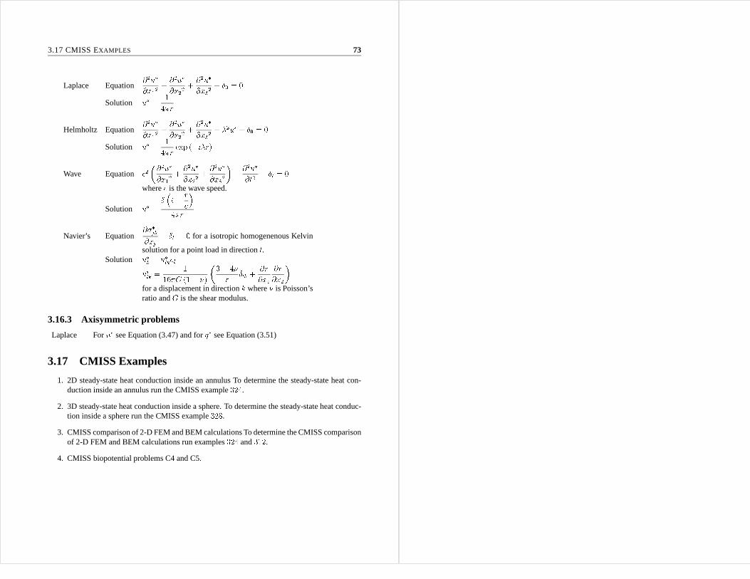
3.17 CMISS EXAMPLES 73
Laplace Equation
@2u�@x12 + @2u�@x22 + @2u�@x32 + �0 = 0
Solution u� = 14�r
Helmholtz Equation
@2u�@x12 + @2u�@x22 + @2u�@x32 + �2u� + �0 = 0
Solution u� = 14�r exp (�i�r)
Wave Equation c2�@2u�@x12 + @2u�@x22 + @2u�@x32�� @2u�@t2 + �t = 0
wherec is the wave speed.
Solution u� = � �t� rc�4�r
Navier’s Equation
@��jk@xj + �l = 0 for a isotropic homogenenous Kelvin
solution for a point load in directionl.Solution u�k = u�lkelu�lk = 116�G (1� �) �3� 4�r �lk + @r@x1 @r@x2�
for a displacement in directionk where� is Poisson’sratio andG is the shear modulus.
3.16.3 Axisymmetric problems
Laplace Foru� see Equation (3.47) and forq� see Equation (3.51)
3.17 CMISS Examples
1. 2D steady-state heat conduction inside an annulus To determine the steady-state heat con-duction inside an annulus run the CMISS example324.
2. 3D steady-state heat conduction inside a sphere. To determine the steady-state heat conduc-tion inside a sphere run the CMISS example328.
3. CMISS comparison of 2-D FEM and BEM calculations To determine the CMISS comparisonof 2-D FEM and BEM calculations run examples324 and312.
4. CMISS biopotential problems C4 and C5.

Chapter 4
Transient Heat Conduction
4.1 Introduction
In the previous discussion of steady state boundary value problems the principal advantage of thefinite element method over the finite difference method has been the greater ease with which com-plex boundary shapes can be modelled. In time-dependent problems the solution proceeds froman initial solution att = 0 and it is almost always convenient to calculate each new solution at aconstant time (t > 0) throughout the entire spatial domain. There is, therefore, no need to usethe greater flexibility (and cost) of finite elements to subdivide the time domain: finite differenceapproximations of the time derivatives are usually preferred. Finite difference techniques are intro-duced in Section 4.2 to solve the transient one dimensional heat equation. A combination of finiteelements for the spatial domain and finite differences for the time domain is used in Section 4.3 tosolve the transient advection-diffusion equation - a slight generalization of the heat equation.
4.2 Finite Differences
4.2.1 Explicit Transient Finite Differences
Consider the transient one-dimensional heat equation@u@t = D@2u@x2 ; (0 < x < L; t > 0) (4.1)
whereD is the conductivity andu = u (x; t) is the temperature, subject to the boundary conditionsu (0; t) = u0 andu (L; t) = u1 and the initial conditionsu (x; 0) = 0. A finite difference approxi-mation of this equation is obtained by defining a grid with spacing�x in the x-domain and�t inthe time domain, as shown in Figure 4.1.
Grid points are labelled by the indicesi = 0; 1; : : : ; I (for thex-direction) andn = 0; 1; : : : ; N(for thet-direction). The temperature at the grid point(i; n) is therefore labelled asu (x; t) = u (i�x; n�t) = uni : (4.2)
Finite difference equations are derived by writing Taylor Series expansions foruni+1; uni�1un+1i
76 TRANSIENT HEAT CONDUCTION
about the grid point(i; n)uni+1 = uni +�x:�@u@x�ni + 12�x2:�@2u@x2�ni + 16�x3:�@3u@x3�ni +O ��x4� (4.3)uni�1 = uni ��x:�@u@x�ni + 12�x2:�@2u@x2�ni � 16�x3:�@3u@x3�ni +O ��x4� (4.4)un+1i = uni +�t:�@u@t �ni +O ��t2� (4.5)
whereO(�x4) andO(�t2) represent all the remaining terms in the Taylor Series expansions.Adding Equations (4.3) and (4.4) givesuni+1 + uni�1 = 2uni +�x2:�@2u@x2�ni +O ��x4�
or �@2u@x2�ni = uni+1 � 2uni + uni�1�x2 +O ��x2� ; (4.6)
which is a “central difference” approximation of the secondorder spatial derivative.Rearranging Equation (4.5) gives a “difference” approximation of the first order time derivative�@u@t�ni = un+1i � uni�t +O(�t) : (4.7)
Substituting Equation (4.6) and Equation (4.7) into the transient heat equation Equation (4.1)gives the finite difference approximationun+1i � uni�t +O(�t) = Duni+1 � 2uni + uni�1�x2 +O ��x2�
which is rearranged to give an expression forun+1i in terms of the values ofu at thenth time stepun+1i = uni +D �t�x2 �uni+1 � 2uni + uni�1�+O ��t2;�x2� : (4.8)
Given the initial values ofuni at n = 0 (i.e., t = 0), the values ofun+1i for the next time stepare found from Equation (4.8) withi = 1; 2; : : : ; I. Applying Equation (4.8) iteratively for timestepsn = 1; 2; : : : etc. yields the time dependent temperatures at the grid points (see Figure 4.1).This is an explicit finite difference formula because the value ofuni depends only on the values ofuni (i = 1; 2; : : : ; I) at the previous time step and not on the neighbouring termsun+1i+1 andun+1i�1 atthe latest time step. The accuracy of the solution depends onthe chosen values of�x and�t andin fact the stability of the scheme depends on these satisfying theCourantcondition:D �t�x2 � 12 : (4.9)

4.2 FINITE DIFFERENCES 77
x
0 10
xx x
i� 1...2n + 1n
ti i+ 1 I x...
1:FIGURE 4.1: A finite difference grid for the solution of the transient 1D heat equation. The
equation is centred at grid point(i; n) shown by theO. The lightly shaded region shows where thesolution is known at time stepn. With central differences inx and a forward difference int anexplicit finite difference formula gives the solution at time stepn+ 1 explicitly in terms of the
solution at the three points below it at stepn, as indicated by the dark shading.
4.2.2 Von Neumann Stability Analysis
The concept behind the Von Neumann analysis is that all Fourier components decay as time ad-vances or as they are processed by an iterative solver. Considering Equation (4.8), we can rearrangethis to be of the form, un+1i = �uni+1 + (1� 2�)uni +�uni�1 (4.10)
where� = D �t�x2 . By subsituting the general Fourier componentunj = Ankei(�kj�xL ), we obtain,An+1k ei(�kj�xL ) = Ank h�ei(�k(j+1)�xL ) + (1� 2�) ei(�kj�xL ) + �ei(�k(j�1)�xL )i (4.11)
If divide Equation (4.11) by,Ankei(�kj�xL ) we obtain (no sum onk),An+1kAnk = (1� 2�) + �ei(�k�xL ) + �e�i(�k�xL )= 1� 2� + 2�cos��k�xL �
using cos(x) = eix + e�ix2= 1� 4�sin2��k�x2L �
using cos(2x) = 1� 2sin2(x) (4.12)
Equation (4.12) predicts the growth of any component (specified byk) admitted by the system.
78 TRANSIENT HEAT CONDUCTION
If all components are to decay,����An+1kAnk ���� � 1 for stability (no sum onk) (4.13)
Since thesin2 term in Equation (4.12) is always between0 and1, we effectively have the stablitycriteria that 1� 4� � 1 and 1� 4� � �1 (4.14)
The first inequality is trivially satisfied, since� � 0 for positive values of�t andD, and thesecond condition will always hold if � = D �t�x2 � 12 (4.15)
Thus, to ensure stability, the time step should be chosen such that�t � �x22D TheCourantcondition (4.16)
4.2.3 Higher Order Approximations
An improvement in accuracy and stability can be obtained by using a higher order approximation
for the time derivative. For example, if a central difference approximation is used for
@u@t by
centering the equation at(i�x; �n+ 12��t) rather than(i�x; n�t) we get�@u@t �n+ 12i = un+1i � uni�t +O ��t2� (4.17)
in place of Equation (4.7) and Equation (4.1) is approximated with the “Crank-Nicolson”formulaun+1i � uni�t = D(12 �@2u@x2�n+1i + 12 �@2u@x2�ni) (4.18)
in which the spatial second derivative term is weighted by12 at the old time stepn and by12 at thenew time stepn + 1. Notice that the finite difference time derivative has not changed - only thetime position at which it is centred. The price paid for the better accuracy (for a given�t) andunconditional stability (i.e., stable forany �t) is that Equation (4.18) is animplicit scheme - theequations for the new time step are now coupled in thatun+1i depends on the neighbouring termsun+1i+1 andun+1i�1 . Thus each new time step requires the solution of a system of coupled equations.
A generalization of (4.18) isun+1i � uni�t = D(��@2u@x2 i�n+1 + (1� �)�@2u@x2 i�n)
(4.19)

4.3 THE TRANSIENT ADVECTION-DIFFUSION EQUATION 79
xx
x
0 x
x x
xn
...2 i + 1
n + 10 1 ii� 1 I
t
:
...
1
FIGURE 4.2: An implicit finite difference scheme based on central differences int, as well asx,
which tie together the 6 points shown byx. The equation is centred at the point (i; n+ 12 ) shown
by theO. The lightly shaded region shows where the solution is knownat time stepn. The darkshading shows the region of the coupled equations.
in which the spatial second derivative of Equation (4.1) hasbeen weighted by� at the new time stepand by(1� �) at the old time step. The original explicit forward difference scheme Equation (4.8)is recovered when� = 0 and the implicit central difference (Crank-Nicolson) scheme (4.19) when� = 12 . An implicit backward difference scheme is obtained when� = 1.
In the following section the transient heat equation is approximated for numerical analysisby using finite differences in time and finite elements in space. We also generalize the partialdifferential equation to include an advection term and a source term.
4.3 The Transient Advection-Diffusion Equation
Consider a linear parabolic equation@u@t + v � ru = Dr2u+ f (4.20)
whereu is a scalar variable (e.g., the advection-diffusion equation, whereu is concentration ortemperature;v � ru then represents advective transport by a velocity fieldv; D is the diffusivityandf is source term. The ratio of advective to diffusive transport is characterised by thePecletnumberV L=D whereV = kvk2 andL is a characteristic length).
Applying the Galerkin weighted residual method to Equation(4.20) with weight! givesZ �@u@t + v � ru�Dr2u� f�! d = 0
80 TRANSIENT HEAT CONDUCTION
or Z ��@u@t + v � ru�! +Dru � r!� d = Z f! d +D Z@ @u@n! d� (4.21)
where
@@n is the normal derivative to the boundary@.
Puttingu = 'nun and! = 'm and summing the element contributions to the global equations,Equation (4.21) can be represented by a system of first order ordinary differential equations,M dudt +Ku =Ku1 (4.22)
whereM is the global mass matrix,K the global stiffness matrix andu a vector of global nodalunknowns with steady state values (t ! 1) u1 . The element contributions toM andK aregiven by Mmne = 1Z0 'm'nJ d� (4.23)
and Kmne = 1Z0 D@'m@�i @'n@�j � @�i@xk @�j@xkJ d� + 1Z0 vj'm@'n@�i @�i@xj J d� (4.24)
If the time domain is now discretized(t = n�t; n = 0; 1; 2; : : :) Equation (4.22) can be re-placed by Mun+1 � un�t +K ��un+1 + (1� �)un� =Ku1 0 � � � 1 (4.25)
where� is a weighting factor discussed in Section 4.2. Note that for� = 12 the method is known
as theCrank-Nicolson-Galerkinmethod and errors arising from the time domain discretization areO(�t2). Rearranging Equation (4.25) as[M + ��tK]un+1 = [M � (1� �)�tK]un +�tKu1 (4.26)
gives a set of linear algebraic equations to solve at the new time step(n+ 1)�t from the knownsolutionun at the previous time stepn�t.
The stability of the above scheme can be examined by expanding u (assumed to be smoothlycontinuous in time) in terms of the eigenvectorssi (with associated eigenvalues�i) of the matrixA = M�1K. Writing the initial conditionsu(0) = Xi aisi and steady state solutionu1 =

4.3 THE TRANSIENT ADVECTION-DIFFUSION EQUATION 81Xi bisi , the set of ordinary differential equations Equation (4.22) has solutionu =Xi �bi + (ai � bi) e��it� si (4.27)
The time-difference scheme Equation (4.26) on the other hand, withu now replaced by a setof discrete valuesun at each time stepn�t, can be written as the recursion formula[I + ��tA]un+1 = [I � (1� �)�tA]un +�tAu1 (4.28)
with solution u =Xi �bi + (ai � bi) �1��t (1� �)�i1 + �t��i �n� si (4.29)
(You can verify that Equation (4.27) and Equation (4.29) areindeed the solutions of Equation (4.22)and Equation (4.25), respectively, by substituting and usingAsi = �isi.)
Comparing Equation (4.27) and Equation (4.29) shows that replacing the ordinary differentialequations (4.22) by the finite difference approximation Equation (4.25) is equivalent to replacingthe exponentiale��it in Equation (4.27) by the approximatione��it � �1��t (1� �)�i1 + �t��i �n
(4.30)
or, with t = n�t, e��it � 1��t (1� �)�i1 + �t��i = 1� �t�i1 + �t��i (4.31)
The stability of the numerical time integration scheme can now be investigated by examiningthe behaviour of this approximation to the exponential. Forstability we require�1 � 1� �t�i1 + �t��i � 1 (4.32)
since this term appears in Equation (4.29) raised to the power n. The right hand inequality inEquation (4.32) is trivially satisfied, since�t; �i and� are all positive, and the left hand inequalitygives �t�i1 + �t��i � 2 or �t�i (1� 2�) � 2 (4.33)
A consequence of Equation (4.33) is that the scheme isunconditionally stableif 12 � � � 1.For� < 12 thestability criterion is �t�i < 21� 2� (4.34)
82 TRANSIENT HEAT CONDUCTION
If the exponential approximation given by Equation (4.31) is negative for any�i the solutionwill contain components which change sign with each time step n. This oscillatory noisecan beavoided by choosing �t < 1(1� �)�max
; (4.35)
where�max is the largest eigenvalue in the matrixA, but in practice this imposes a limit whichis too severe for�t and a small amount of oscillatory noise, associated with thehigh frequencyvibration modes of the system, is tolerated. Alternativelythe oscillatory noise can be filtered outby averaging.
These theoretical results are explored numerically with a Crank-Nicolson-Galerkin scheme(� = 12 ) in Figure 4.3, where the one-dimensional diffusion equation@u@t = D@2u@x2 on 0 � x � 1
subject to initial conditions u (x; 0) = 0
and boundary conditions u (0; t) = 0; u (1; t) = 1 (4.36)
is solved for various time increments (�t) and element lengths (�x) for both linear and cubicHermite elements.
Decreasing�x from 0:25 to 0:1 with linear elements produces more oscillation because thesystem has more degrees of freedom and leads to greater oscillation. At a sufficiently small�t theoscillations are negligible (bottom right, Figure 4.3). With this value of�t (0:01 s) the numericalresults agree well with the exact solution (top, Figure 4.3)given byu (x; t) = x + 2� 1Xn=1 (�1)nn e�n2�2t sin (n�x) (4.37)
4.4 Mass lumping
A technique known asmass lumpingis sometimes used in which the mass matrixM is replacedby a diagonal matrix having diagonal terms equal to the row sums. For example, consider the mass

4.4 MASS LUMPING 83
�x = 0:1linear elements
x
x
x
x
x
(d) x = 0:9
x
xx
xlinear elements�x = 0:1x
x
x
xx
xx
x
x
xx
x
xx x
cubic elements
(c) x = 0:75
�t = 0:1
x x
0:5
11
11u
ut =1
Linear CNG with�x = 0:1;�t = 0:01x x1:0t = 0:1t = 0:02 t = 0:05
u(x; t)u0
00
(e)x = 0:9�t = 0:01
xx
0
u
tt
t
0 1 x
t �t = 0:1
x
Exact solution
x
xxxxx
x
x
x �x = 0:25x
x�t = 0:1x
(b) x = 0:75
linear elements�x = 0:25
x
x
x
xxx xx
x
x
x
x
x
x x
x
x
FIGURE 4.3: Analytical and numerical solutions of the transient 1Dheat equation showing theeffects of element size�x and time step size�t. The top graph shows the exact and approximatesolutions as functions ofx at various times. The lower graphs show the solution throughtime at the
specifiedx positions and with various choices of�x and�t as indicated.
84 TRANSIENT HEAT CONDUCTION
matrix (Equation (4.23)) for a bilinear element (see Figure1.9 and Equation (1.6)).M11 = ZZ (1� �1)2 (1� �2)2�1�2 = �(1� �1)33 �����0 1 �(1� �2)33 �����0 1 = 13 � 13 = 19M22 = ZZ �21 (1� �2)2�1�2 = 13 � 13 = 19 and similarlyM33 andM44.M12 = ZZ �1 (1� �1) (1� �1)2�1�2 = ��12 � 13� � 13 = 118M13 = ZZ (1� �1)2 �2 (1� �2)�1�2 = 118 and similarlyM34 andM24.M14 = ZZ �1 (1� �1) �2 (1� �2)�1�2 = 136 and similarlyM23.thereforeM = 2664 19 118 118 136118 19 136 118118 1136 19 118136 118 118 19 3775 mass lumping�! 266414 0 0 00 14 0 00 0 14 00 0 0 143775
The element mass is effectively lumped at the element vertices. Such a scheme has computa-tional advantages when� = 0 in Equation (4.26) because each component of the vectorun+1 isobtained directly without the need to solve a set of coupled equations. Thisexplicit time integrationscheme, however, is only conditionally stable (see (4.34))and suffers fromphase lag errors- seebelow. For evenly spaced elements the finite element scheme with mass lumping is equivalent tofinite differences with central spatial differences.
In Figure 4.4, the finite element and finite differences (lumped f.e. mass matrix) solutions of theone-dimensional advection-diffusion equation (4.20) with V = 5 m s�1, D = 0:1 m2s�1, f = 0
are compared for the propogation and dispersion of an initial unit mass pulse atx = 0. The lengthof the solution domain is sufficient to avoid reflected end effects.
The exact solution is a Gaussian distribution whose variance increases with time:u (x; t) = Mp4��te�(x� V t)24Dt (4.38)
The finite element solution, using the Crank-Nicolson-Galerkin technique, shows excellentamplitude and phase characteristics when compared with theexact solution. The finite difference,or lumped mass, solution also using centered time differences, reproduces the amplitude of thepulse very well but shows a slight phase lag.
4.5 CMISS Examples
1. To solve for the transient heat flow in a plate run CMISS example331
2. To investigate the stability of time integration schemesrun CMISS examples3321 and3322.

4.5 CMISS EXAMPLES 85
oo
oo
o
o
ox
x x
oo
o
ot = 0:2 s t = 0:4 sV = 5 m s�1
xD = 0:1 m2 s�1u (x; t)
t = 0:05 s Finite difference solution
Finite element solutionxx
Exact solution
t = 0:01 s
x
x
x x
x x
xx xx
xx
xx x
x
xxx
x
FIGURE 4.4: Advection-diffusion of a unit mass pulse. The finite element solutions (att=0:01 s,0:05 s, 0:2 s and0:4 s) and finite difference solutions (att=0:4 s only) are compared with the exactsolution.�x= 0.1,�t = 0:001 s for 0< t <0:01 s and�t = 0.01 fort � 0:01 s.

Chapter 5
Linear Elasticity
5.1 Introduction
To analyse the stress in various elastic bodies we calculatethe strain energy of the body in terms ofnodal displacements and then minimize the strain energy with respect to these parameters - a tech-nique known as the Rayleigh-Ritz. In fact, as we will show later, this leads to the same algebraicequations as would be obtained by the Galerkin method (now equivalent to virtual work) but thephysical assumptions made (in neglecting certain strain energy terms) are exposed more clearly inthe Rayleigh-Ritz method. We will first consider one-dimensional truss and beam elements, thentwo-dimensional plane stress and plane strain elements, and finally three-dimensional elasticity.
In all cases the steps are:
1. Evaluate the components of strain in terms of nodal displacements,
2. Evaluate the components of stress from strain using the elastic material constants,
3. Evaluate the strain energy for each element by integrating the products of stress and straincomponents over the element volume,
4. Evaluate the potential energy from the sum of total strainenergy for all elements togetherwith the work done by applied boundary forces,
5. Apply the boundary conditions,e.g.,by fixing nodal displacements,
6. Minimize the potential energy with respect to the unconstrained nodal displacements,
7. Solve the resulting system of equations for the unconstrained nodal displacements,
8. Evaluate the stresses and strains using the nodal displacements and element basis functions,
9. Evaluate the boundary reaction forces (or moments) at thenodes where displacement isconstrained.
88 L INEAR ELASTICITY
5.2 Truss Elements
Consider the one-dimensional truss of undeformed lengthL in Figure 3.1 with end points(0; 0)
and (x; y) and making an angle� with the x-axis. Under the action of forces in thex- andy-directions the right hand end of the truss displaces byu in thex-direction andv in they-direction,relative to the left hand end.
L u(X; Y ) (X + u; Y + v)x
y�
vl
FIGURE 5.1: A truss of initial lengthL is stretched to a new lengthl. Displacements of the righthand end relative to the left hand end areu andv in thex- andy- directions, respectively.
The new length isl with axial straine = lL � 1 = q(X + u)2 + (Y + v)2pX2 + Y 2 � 1= pL2 + 2 (Xu+ Y v) + u2 + v2L � 1=r1 + 2�cos �: uL + sin �: vL�+ u2 + v2L2 � 1
using
XL = cos � and
YL = sin �, where� is defined to be positive in the anticlockwise direction.
Neglecting second order terms in the binomial expansion
p(1 + ") = 1 + 12"+O("2), the strain
for small displacementsu andv is e �= cos �: uL + sin �: vL (5.1)

5.2 TRUSSELEMENTS 89
The strain energy associated with this uniaxial stretch is
SE= 12 Z �e dV = 12A LZ0 �e dx = 12 LZ0 EAe2 dx = 12ALEe2 (5.2)
where� = Ee is the stress in the truss (of cross-sectional areaA), linearly related to the straine
via Young’s modulusE. We now substitute fore from Equation (5.1) into Equation (5.2) and putu = u2 � u1 andv = v2 � v1, where(u1; v1) and(u2; v2) are the nodal displacements of the twoends of the truss
SE= 12ALE �cos �:u2 � u1L + sin �:v2 � v1L �2
(5.3)
The potential energy is the combined strain energy from all trusses in the structure minus thework done on the structure by external forces. The Rayleigh-Ritz approach is to minimize thispotential energy with respect to the nodal displacements once all displacement boundary conditionshave been applied.
For example, consider the system of three trusses shown in Figure 5.2. A force of100 kN
is applied in thex-direction at node1. Node2 is a sliding joint and has zero displacement in they-direction only. Node3 is a pivot and therefore has zero displacement in bothx- andy- directions.The problem is to find all nodal displacements and the stress in the three trusses.
30� 213
node130�
100 kN
node3 node2
FIGURE 5.2: A system of three trusses.
The strain in truss1 (joining nodes1 and3) isu1L cos 30 + v1L sin 30 = p32 u1L + 12 v1LThe strain in truss2 (joining nodes1 and2) is(u1 � u2)L cos 90 + v1L sin 90 = v1L
90 L INEAR ELASTICITY
The strain in truss3 (joining nodes2 and3) isu2L cos (�30) = p32 u2LSince a force of100 kN acts at node1 in thex-direction, the potential energy is
PE= X
trusses
12ALEe2 � 100u1 = 12AEL 24 p32 u1 + 12v1!2 + p32 u2!2 + (v1)235� 100u1
[Note that if the force was applied in the negativex-direction, the final term would be+100u1]Minimizing the potential energy with respect to the three unknownsu1, v1 andu2 gives@PE@u1 = AEL p32 u1 + 12v1! p32 � 100 = 0 (5.4)@PE@v1 = AEL " p32 u1 + 12v1! 12 + v1# = 0 (5.5)@PE@u2 = AEL p32 u2! p32 = 0 (5.6)
If we chooseA = 5 � 10�3 m2, E = 10 GPa andL = 1 m (e.g.,100 mm � 50 mm timber
truss) then
AEL = 5� 10�3 m2 �107 kPa=m = 5� 104 kN m�1.Equation (5.6) gives u2 = 0
Equation (5.4) gives 3u1 +p3v1 = 4� 102= �5� 104�
Equation (5.5) gives for two dimensionsv1 = �p35 u1
Solving these last two equations givesu1 = 3:34 mm andv1 = �1:15 mm. Thus the strain in truss1 is (p32 3:34� 121:15)� 10�3 = 0:232%, in truss2 is�0:115% and in truss3 is zero.
The tension in truss1 isA� = AEe = 5�10�3 m2107 kPa�0:232�10�2 = 116 kN (tensile),in truss2 is�57:5 kN (compressive) and in truss3 is zero. The nodal reaction forces are shown inFigure 5.3.

5.3 BEAM ELEMENTS 91
100 kN 57:7 kN 57:7 kN100 kN
FIGURE 5.3: Reaction forces for the truss system of Figure 5.2.
5.3 Beam Elements
Simple beam theory ignores all but axial strainex and stress�x = Eex (E = Young’s modulus)
along the beam (assumed here to be in the x-direction). The axial strain is given byex = zR ,
wherez is the lateral distance from the neutral axis in the plane of the bending andR is the radius
of curvature in that plane. The bending moment is given byM = Z �xz dA , whereA is the beam
crossectional area. Thus �x = Eex = E zR (5.7)M = Z �xz dA = ER Z z2 dA = EIR (5.8)
whereI = Z z2 dA is the second moment of area of the beam cross-section. Thus,
ER = MI and
Equation (5.7) becomes �x = MzI (5.9)
The slope of the beam is
dwdx = � and the rate of change of slope is the curvatureK = d�dx = d2wdx2 = 1R (5.10)
92 L INEAR ELASTICITY
Thus the bending moment is M = EI d2wdx2 = EIw00 (5.11)
and a force balance gives the shear forceV = �dMdx = � ddx (EIw00) (5.12)
and the normal force (per unit length of beam)p = dVdx = � d2dx2 (EIw00) (5.13)
This last equation is the equilibrium equation for the beam,balancing the loading forcesp with theaxial stresses associated with beam flexure� d2dx2 �EI d2wdx2 � = p (5.14)
The elastic strain energy stored in a bent beam is the sum of flexural strain energy and shearstrain energy, but this latter is ignored in the simple beam theory considered here. Thus, the(flexural) strain energy is
SE= 12 LZx=0 ZA �xex dA dx = 12 LZx=0 E ZA e2x dA dx= 12 LZx=0 E ZA � zR�2 dA dx = 12 LZx=0 EI (w00)2 dx
wherex is taken along the beam andA is the cross-sectional area of the beam.The external work associated with forcesp acting normal to the beam and moving through a
transverse displacementw is
LZ0 pw dx. The potential energy is therefore
PE= 12 LZ0 EI (w00)2 dx� LZ0 pw dx: (5.15)
The finite element approximation for the transverse displacementw must be able to representthe second derivativew00. A linear basis function has a zero second derivative and therefore cannotrepresent the flexural strain. The natural choice of basis function for beam deflection is in fact cubicHermite because the inter-element slope continuity of thisbasis ensures transmission of bendingmoment as well as shear force across element boundaries.
The boundary conditions associated with the4th order equilibrium Equation (5.14) or the equa-

5.4 PLANE STRESSELEMENTS 93
tions arising from minimum potential energy Equation (5.15) (which contain the square of2nd
derivative terms) are more complex than the simple temperature or flux boundary conditions forthe (second order) heat equation. Three possible combinations of boundary condition with theirassociated reactions are
Boundary conditions Reactions
(i) Simply supported zero displacementw = 0 shear forceV
zero momentM = EIw00 = 0 slope�(= w0)
(ii) Cantilever zero displacementw = 0 shear forceV
zero slope� = w0 = 0 momentM
(iii) Free end zero shear forceV = � ddx (EIw00) = 0 displacementw
zero momentM = EI 00 = 0 slope�
5.4 Plane Stress ElementsFor two-dimensional problems, we define the displacement vector u = �uv�, strain vectore =24 exeyexy35 and stress vector� = 24 �x�y�xy35. The stress-strain relation for two-dimensional plane stress:�x = E1� �2 (ex + �ey)�y = E1� �2 (ey + �ex)�xy = E1 + � (exy) (5.16)
can be written in matrix form � = Ee
whereE = E1� �2 241 � 0� 1 00 0 1� �35. The strain components are given in terms of displacement
gradients by ex = @u@xey = @v@yexy = 12 �@u@y + @v@x� (5.17)
94 L INEAR ELASTICITY
The strain energy is
SE= 12 ZV �Te dV = 12 ZV (ex�x + ey�y + exy�xy) dV= 12 ZV eTEe dV = 12 ZV E1� �2 �e2x + e2y + 2�exey + (1� �) e2xy� dV
The potential energy is
PE= SE� external work= 12 ZV eTEe dV � ZA uT l dA (5.18)
wherel represents the external loads (forces) acting on the elastic body.Following the steps outlined in Section 5.1 we approximate the displacement fieldu with a
finite element basisu = 'nun, v = 'nvn and calculate the strainsex = @u@x = @'n@x uney = @v@y = @'n@y vnexy = 12 �@u@y + @v@x� = 12 �@'n@y un + @'n@x vn� (5.19)
or e = 24 exeyexy35 = 2666664 @'n@x 00 @'n@y12 @'n@y 12 @'n@x3777775�unvn� = Bu (5.20)
From Equation (5.18) the potential energy is therefore
PE= 12 ZV (Bu)TE (Bu) dV � ZA uT l dA= 12uT 24ZV BTEB dV 35u� ZA uT l dA= 12uTKu� ZA uT l dA

5.4 PLANE STRESSELEMENTS 95
whereK = ZV BTEB dV is the element stiffness matrix.
We next minimize the potential energy with respect to the nodal parametersun andvn givingKu = f (5.21)
wheref = ZA l dA is a vector of nodal forces.
5.4.1 Notes on calculating nodal loads
If a known stress acts normal to a given surface (e.g.,a surface pressure), it may be applied bycalculating equivalent nodal forces. For example, consider a uniform loadp kN m�1 applied to theedge of the plane stress element in Figure 5.4a.
The nodal load vectorf in Equation (5.21) has componentsfn = Zx p'n dx = pL 1Z0 'n d� (5.22)
where� is the normalized element coordinate along the side of length L loaded by the constantstressp kN m�1. If the element side has a linear basis, Equation (5.22) givesf1 = pL 1Z0 '1 d� = pL 1Z0 (1� �) d� = 12pLf2 = pL 1Z0 '2 d� = pL 1Z0 � d� = 12pL
as shown in Figure 5.4b. If the element side has a quadratic basis, Equation (5.22) givesf1 = pL 1Z0 '1 d� = pL 1Z0 2�12 � �� (1� �) d� = 16pLf2 = pL 1Z0 '2 d� = pL 1Z0 4� (1� �) d� = 23pLf3 = pL 1Z0 '3 d� = pL 1Z0 2��� � 12� d� = 16pLas shown in Figure 5.4c. A node common to two elements will receive contributions from bothelements, as shown in Figure 5.4d.
96 L INEAR ELASTICITY
(a) (b)
16pL12pL
12pL 13p �L2 �23p �L2 �16p �L2 �23pL(c) (d)
p kN m�1 16p �L2 �23p �L2 �L 16pLFIGURE 5.4: A uniform boundary stress applied to the element side in(a) is equivalent to nodalloads of12pL and 12pL for the linear basis used in (b) and to16pL, 23pL and 16pL for the quadratic
basis used in (c). Two adjacent quadratic elements both contribute to a common node in (d), wherethe element length is nowL2 .
5.5 Three-Dimensional Elasticity
Consider a surface� enclosing a volume of material of mass density�. Conservation of linearmomentum over the domain results in the governing stress equilibrium equations�ij;j + bi = 0 i; j = 1; 2; 3 (5.23)
where�ij are the components of the stress tensor (�ij is the component of the traction or stressvector in theith direction which is acting on the face of a rectangle whose normal is in thej th
direction), andbi is the body force/unit volume (e.g.,b = �g). Note that the notation�ij;j = @�ij@xj
has been introduced to represent the derivative.Recall that the components of the linear (or small) strain tensor areeij = 12 (ui;j + uj;i) i; j = 1; 2; 3 (5.24)
whereu is the displacement vector (i.e.,u is the difference between the final and initial positionsof a material point in question). Note: we are assuming here that the displacement gradients aresmall compared to unity, which is appropriate for many materials in solid mechanics. However, forsoft materials, such as rubber or biological tissue, then weneed to use the exact finite strain tensor.
The object of solving an elasticity problem is to find the distributions of stress and displacementin an elastic body, subject to a known set of body forces and prescribed stresses or displacementsat the boundaries. In the general three-dimensional case, this means finding6 stress components�ij (= �ji which arises from the conservation of angular momentum) and3 displacementsui eachas a function of position in the body. Currently we have15 unknowns (6 stresses,6 strains and3
displacements), but only9 equations (3 equilibrium equations and6 strain-displacement relations).To progress, we require an equation of state,i.e.,a stress-strain relation or constitutive law. For
a linear elastic material we may propose that the componentsof stress�ij depend linearly oneij.

5.5 THREE-DIMENSIONAL ELASTICITY 97
i.e., �ij = cijklekl
wherecijkl are the81 components of a4th order tensor, although symmetry of the strain and stresstensors reduces the number of independent components to21.
If the material is assumed to be isotropic (i.e., the material response is independent of orienta-tion of the material element), then we end up with the generalized Hooke’s Law.�ij = �ekk�ij + 2�eij (5.25)
or inversely eij = 12��ij � �2� (3�+ 2�)�kk�ij
where�, � are Lames constants.Note:�, � are related to Young’s modulesE and Poisson’s ratio� byE = � (3�+ 2�)�+ �� = �2 (�+ �)
Providing that the displacements are continuous functionsof position, then Equation (5.23),Equation (5.24) and Equation (5.25) are sufficient to determine the15 unknown quantities. Thiscan often work with some smaller grouping or simplification of these equations,e.g.,if all bound-ary conditions are expressed in terms of displacements, substituting Equation (5.24) into Equa-tion (5.25) then into Equation (5.23) yields Navier’s equation of motion.�ui;kk + (�+ �)uk;ki + bi = 0 i; k = 1; 2; 3These3 equations can be solved for the unknown displacements. ThenEquation (5.24) can be usedto determine the strains and Equation (5.25) to calculate the stresses.
5.5.1 Weighted Residual Integral Equation
Using weighted residuals as before we can writeZ (�ij;j + bi)u�i d = 0 (5.26)
whereu� = (u�i ) is a (vector) weighting field. Theu�i are usually interpreted as a consistent set ofvirtual displacements (hence we use the notationu instead ofw).
98 L INEAR ELASTICITY
By the chain-rule (�iju�i );j = �ij;ju�i + �iju�i;jTherefore, the first term in the integrand of Equation (5.26)can be re-writtenZ �ij;ju�i d = Z (�iju�i );j d� Z �iju�i;j d= Z r � (�iju�i ) d� Z �iju�i;j d= Z@ �iju�inj d�� Z �iju�i;j d (5.27)
where the domain integral involving “r� = @@xj ” has been transformed into a surface integral
using the divergence theoremZ r � g d = Z@ g � n d� or
Z gj;j d = Z@ gjnj d�
wheren = njij is the outward normal vector to the surface�.Thus, combining Equation (5.26) and Equation (5.27) we haveZ �iju�i;j d = Z biu�i d + Z@ �ijnju�i d�= Z biu�i d + Z@ tiu�i d� (5.28)
whereti are the components of the internal stress vector (t) and are related to the components ofthe stress tensor (�ij) by Cauchy’s formulat = �ijnjii (5.29)
To arrive at this point, we have used weighted residuals to tie in with Chapter 2, howeverEquation (5.28) is more usually derived using the principleof virtual work (below). Note that theweighted integral Equation (5.28) is independent of the constitutive law of the material.
5.5.2 The Principle of Virtual Work
The governing equations for elastostatics can also be derived from a physically appealing argument.Let s be the external traction vector (i.e., force per unit surface area). For equilibrium, the workdone by the external surface forcess = siii, in moving through a virtual displacementu� = u�i ii

5.5 THREE-DIMENSIONAL ELASTICITY 99
is equal to the work done by the stress vectort = tiii in moving through a compatible set of virtualdisplacementsu�. In mathematical terms, the principle of virtual work can bewrittenZ@ siu�i d� = Z@ tiu�i d� = Z@ �ijnju�i d� (5.30)
using Cauchy’s formula (Equation (5.29)).The Green-Gauss theorem (Equation (2.15)) is now used to replace the right hand surface
integral in Equation (5.30) by a volume integral, givingZ@ siu�i d� = Z ��ij;ju�i + �iju�i;j� d (5.31)
Substituting the equilibrium relation (Equation (5.23)) into the first integrand on the right handside, yields thevirtual work equationZ �iju�i;j d = Z biu�i d + Z@ siu�i d� (5.32)
where the internal work done due to the stress field is equatedto the work due to internal bodyforces and external surface forces. Note that Equation (5.32) is equivalent to Equation (5.28) viaEquation (5.30). In practice, Equation (5.32) is in a more useful form than Equation (5.28), becausethe right hand side integrals can be expressed in terms of theknown body forces and the appliedboundary conditions (surface traction forces or stresses).
5.5.3 The Finite Element Approximation
Let = S e and interpolate the virtual displacementsu�i from their nodal values.i.e.,u�i = 'm _(umi )�
so u�i;j = @'m@xj _(umi )�= 'm;k @�k@xj _(umi )� (5.33)
where(umi )� = (U4(m;e)i )�,4(m; e) is the global node number of local nodem on elemente, and
the shorthand'm;k = @'m@�k has been introduced.
Substituting this into Equation (5.32) givesXe 0@Ze �ij'm;k @�k@xj d1A�U4(m;e)i �� =Xe 0@Ze bi'm d + Z@e si'm d�1A�U4(m;e)i ��
100 L INEAR ELASTICITY
and since the virtual displacements are arbitrary we getXe Ze �ij'm;k @�k@xj d =Xe 0@Ze bi'm d + Z@e si'm d�1A (5.34)
The next step is to express the stress components�ij in terms of the virtual displacementsand their finite element approximation by substituting Equation (5.33) into Equation (5.24) (thestrain-displacement relation) and in turn into Equation (5.25) (the generalized Hooke’s law).
We first introduce the finite element approximation for the displacement fielduj = 'nunj whichgives eij = 12 � @@xj ('nuni ) + @@xi �'nunj �� = 12 �@'n@�l @�l@xj uni + @'n@�l @�l@xiunj� (5.35)
and ekk = uk;k = @'n@�l @�l@xk unk
Thus �ij = ��ij @'n@�l @�l@xk unk + 2��12 @'n@�l @�l@xj uni + 12 @'n@�l @�l@xiunj�
which, due to symmetry of the stress tensor, simplifies to�ij = ��ij @'n@�l @�l@xk unk + 2�@'n@�l @�l@xiunj= ���i(j)'n;l @�l@xj + 2�'n;l @�l@xi�unj (5.36)
where the summation indexk has been replaced withj, but the parenthesis in�i(j) implies thatthere is no sum with respect to that particular index.
Substituting this expression into Equation (5.34) and simplifying, we get for each elementunj Ze ��'n;l @�l@xj'm;k@�k@xi + 2�'n;l @�l@xi'm;k @�k@xj� d = fim (5.37)
wherefim denotes the right hand side terms in Equation (5.34). (Note that there has been somecareful manipulation of summation indices with the substitution of Equation (5.36) to arrive atEquation (5.37).)
So for each element Eimjnunj = fim

5.6 LINEAR ELASTICITY WITH BOUNDARY ELEMENTS 101
where Eimjn = 1ZZZ0 �� @�l@xj @�k@xi + 2� @�l@xi @�k@xj�'n;l'm;kJ(�1; �2; �3)d�1d�2d�3fim = 1ZZZ0 bi'mJ(�1; �2; �3)d�1d�2d�3 + 1ZZ0 si'mJ2D(�1; �2)d�1d�2 (5.38)
where the JacobiansJ(�1; �2; �3) andJ2D(�1; �2) have been used to transform volume and sur-face integrals so that they can be can be calculated using�-coordinates. (Note: without loss ofgenerality, the above definition offim assumes that(�1; �2) are defined to lie in the surface�.)
So in summary, the finite element approximation leads to element stiffness matrix componentsthat can be calculated from the known material parameters, the chosen interpolation functions, andthe geometry of the material (note that the element stiffness components are independent of theunknown displacement parameters). Element stiffness components are then assembled into theglobal stiffness matrix in the usual manner (as described previously). Note that this is implicitly aGalerkin formulation, since the unknown displacement fields are interpolated using the same basisfunctions as those used to weight the integral equations.
5.6 Linear Elasticity with Boundary Elements
Equation (5.28) is the starting point for the general finite element formulation (Section 5.5). Inthe above derivation, we have essentially used the Green-Gauss theorem once to move from Equa-tion (5.26) to Equation (5.28) (as was done for the derivation of the FEM equation for Laplace’sequation). To continue, we firstly note that�ije�ij = 12�iju�i;j + 12�iju�j;i= 12�iju�i;j + 12�jiu�j;i= 12�iju�i;j + 12�iju�i;j= �iju�i;j
wheree�ij are the virtual strains corresponding to the virtual displacements.
102 L INEAR ELASTICITY
Using the constitutive law for linearly elastic materials (Equation (5.25)) we haveZ �iju�i;j d = Z �ije�ij d= � Z ekke�ij�ij d + 2� Z eije�ij d= � Z ekke�kk d + 2� Z eije�ij d= Z eij��ij ddue to symmetry.
Thus from the virtual work statement, Equation (5.28) and the above symmetry we haveZ biu�i d + Z@ tiu�i d� = Z b�iui d + Z@ t�iui d� (5.39)
This is known as Betti’s second reciprical work theorem or the Maxwell-Betti reciprocity relation-ship between two different elastic problems (the starred and unstarred variables) established on thesame domain.
Note thatb�i = ���ij;j (i.e.,��ij;j + b�i = 0). Therefore Equation (5.39) can be written asZ ���ij;j�ui d + Z biu�i d = Z@ t�iui d�� Z@ tiu�i d� (5.40)
(��ij ; e�ij; t�i represents the equilibrium state corresponding to the virtual displacementsu�i ).Note: What we have essentially done is use integration of parts to get Equation (5.28), then use
it again to get Equation (5.39) above (after noting the reciprocity between�ij andeij).Since the body forces,bi, are known functions, the second domain integral on the lefthand
side of Equation (5.40) does not introduce any unknowns intothe problem (more about this later).The first domain integral contains unknown displacements in and it is this integral we wish toremove.
We choose the virtual displacements such that��ij;j + ei� = 0 (5.41)
(or equivalently�b�i + ei� = 0), whereei is theith component of a unit vector in theith directionandei� = ei� (x� P ). We can interpret this as the body force components which correspond to apositive unit point load applied at a pointP 2 in each of the three orthogonal directions.
Therefore

5.7 FUNDAMENTAL SOLUTIONS 103
Z ��ij;jui d = � Z � (x� P ) eiui d = �ui(P )ei
i.e., the volume integral is replaced with a point value (as for Laplace’s equation).Therefore, Equation (5.40) becomesui (P ) ei = Z@ tju�j d�� Z@ t�juj d� + Z bju�j d P 2 (5.42)
If each point load is taken to be independent thenu�j andt�j can be written asu�j = u�ij (P; x) ei (5.43)t�j = t�ij (P; x) ei (5.44)
whereu�ij (P; x) and t�ij (P; x) represent the displacements and tractions in thej th direction atx
corresponding to a unit point force acting in theith direction (ei) applied atP . Substituting theseinto Equation (5.42) (and equating components in eachei direction) yieldsui (P ) = Z@ u�ij (P; x) tj (x) d� (x)� Z@ t�ij (P; x) uj (x) d� (x)+ Z u�ij (P; x) bj (x) d (x) (5.45)
whereP 2 (see later forP 2 @).This is known as Somigliana’s1 identity for displacement.
5.7 Fundamental Solutions
Recall from Equation (5.41) that��ij satisfied��ij;j + � (x� P ) ei = 0 (5.46)
or equivalently b�i = ei� (x� P )Navier’s equation for the displacementsu�i isG u�i;kk + G1� 2� u�k;ki + b�i = 0
1Somigliana was an Italian Mathematician who published thisresult around 1894-1902.
104 L INEAR ELASTICITY
whereG = shear Modulus.Thusu�i satisfy G u�i;kk + G1� 2� u�k;ki + � (x� P ) ei = 0 (5.47)
The solutions to the above equation in either two or three dimensions are known as Kelvin2’sfundamental solutions and are given byu�ij (P;x) = 116� (1� �)Gr f(3� 4�) �ij + r;ir;jg (5.48)
for three-dimensions and for two-dimensional plane strainproblems,u�ij (P;x) = �18� (1� �)G f(3� 4�) �ij log r � r;ir;jg (5.49)
andt�ij (P;x) = �14�� (1� �) r� �((1� 2�) �ij + �r;ir;j) @r@n � (1� 2�) (r;inj � r;jni)� (5.50)
where� = 1; 2; � = 2; 3 for two-dimensional plane strain and three-dimensional problems respec-tively.
Herer � r (P;x), the distance between load point (P ) and field point (x), ri = xi (x)�xi (P )
andr;i = @r@xi (x) = rir .
In addition the strains at an pointx due to a unit point load applied atP in theith direction aregiven bye�jki (P;x) = �18�� (1� �)Gr� f(1� 2�) (r;k�ij + r;j�ik)� r;i�jk + �r;ir;jr;kg
and the stresses are given by��ijk (P;x) = �14�� (1� �) r� f(1� 2�) (r;k�ij + r;j�ki � r;i�jk) + �r;ir;jr;kg
where� and� are defined above.The plane strain expressions are valid for plane stress if� is replaced by� = �1 + � (This is a
mathematical equivalence of plane stress and plane strain -there are obviously physical differences.What the mathematical equivalence allows us to do is to use one program to solve both types ofproblems - all we have to do is modify the values of the elasticconstants).
Note that in three dimensionsu�ij = O�1r� t�ij = O� 1r2�
2Lord Kelvin (1824-1907) Scottish physicist who made great contributions to the science of thermodynamics

5.8 BOUNDARY INTEGRAL EQUATION 105
and for two dimensions u�ij = O(log r) t�ij = O�1r� :
Somigliana’s identity (Equation (5.45)) is a continuous representation of displacements at anypointP 2 . Consequently, one can find the stress at anyP 2 firstly by combining derivativesof (5.45) to produce the strains and then substituting into Hooke’s law. Details can be found inBrebbia, Telles & Wrobel (1984b) pp 190–191, 255–258.
This yields�ij (P ) = Z� u�ijk (P;x) tk (x) d� (x)� Z� t�ijk (P;x) uk (x) d� (x)+ Z u�ijk (P;x) bk (x) d (x)
Note: One can find internal stress via numerical differentiation as in FE/FD but these are notas accurate as the above expressions.
Expressions for the new tensorsu�ijk andt�ijk are on page 191 in (Brebbia et al. 1984b).
5.8 Boundary Integral Equation
Just as we did for Laplace’s equation we need to consider the limiting case of Equation (5.45) asP is moved to@. (i.e.,we need to find the equivalent ofc (P ) (in section 3) - called herecij (P ).)We use the same procedure as for Laplace’s equation but here things are not so easy.
If P 2 @ we enlarge to0 as shown.
0 �""P ��"
FIGURE 5.5: Illustration of enlarged domain when singular point ison the boundary.
106 L INEAR ELASTICITY
Then Equation (5.45) can be written asui (P ) = Z��"+�" u�ij (P;x) tj (x) d� (x)� Z��"+�" t�ij (P;x) uj (x) d� (x)+ Z0 u�ij (P;x) bj (x) d (x) (5.51)
We need to look at each integral in turn as"#0 (i.e.,"! 0 from above). The only integral thatpresents a problem is the second integral. This can be written asZ��"+�" t�ij (P;x) uj (x) d� (x) = Z�" t�ij (P;x) uj (x) d� (x)+ Z��" t�ij (P;x) uj (x) d� (x) (5.52)
The first integral on the right hand side can be written asZ�" t�ij (P;x) uj (x) d� (x) = Z�" t�ij (P;x) [uj (x)� uj (P )] d�(x)| {z }0 by continuity ofuj (x)+ uj (P )Z�" t�ij (P;x) d� (x) (5.53)
Let cij (P ) = �ij + lim"#0 Z�" t�ij (P;x) d� (x) (5.54)
As"#0,��" ! � and we write the second integral of Equation (5.52) as
Z� t�ij (P;x)uj (x) d� (x)
where we interpret this in the Cauchy Principal Value3sense.
3What is a Cauchy Principle Value?
Considerf (x) = 1x on��" = [�2;�") [ ("; 2]

5.8 BOUNDARY INTEGRAL EQUATION 107
Thus as"#0 we get the boundary integral equationcij (P )uj (P ) + Z� t�ij (P;x)uj (x) d� (x)= Z� u�ij (P;x) tj (x) d� (x) + Z u�ij (P;x) bj (x) d (5.55)
(or, in brief (no body force),cijuj + Z� t�ijuj d� = Z� u�ijtj d�) where the integral on the left hand
side is interpreted in the Cauchy Principal sense. In practical applicationscij and the principal valueintegral can be found indirectly from using Equation (5.55)to represent rigid-body movements.
The numerical implementation of Equation (5.55) is similarto the numerical implementationof an elliptic equation (e.g.,Laplace’s Equation). However, whereas with Laplace’s equation the
unknowns wereu and
@u@n (scalar quantities) here the unknowns are vector quantities. Thus it is
more convenient to work with matrices instead of indicial notation.i.e.,use u = 24u1u2u335 ; t = 24t1t2t335u� = 24u�11 u�12 u�13u�21 u�22 u�23u�31 u�32 u�3335 ; t� = 24t�11 t�12 t�13t�21 t�22 t�23t�31 t�32 t�3335
ThenZ��" f (x) dx = �"Z�2 1x dx+ 2Z" 1x dx = ln jxjj�"�2 + ln jxjj2"= ln "� ln 2 + ln 2� ln " = 0 8" > 0) lim"!0 Z��" f (x) dx = 0 This is the Cauchy Principle Value of
Z� f (x) dxBut if we replace��" by lim"!0��" = [�2; 2] = � thenZ� 1x dx = 2Z�2 1x dx = 0@ lim"1!0 "1Z�2 1x dx1A+0@ lim"2!0 2Z�"2 1x dx1A(by definition of improper integration)
which does NOT exist.i.e., the integral does not exist in the proper sense, but it does inthe Cauchy Principal Valuesense. However, if an integral exists in the proper sense, then it exists in the Cauchy Principal Value sense and the twovalues are the same.
108 L INEAR ELASTICITY
Then (in absence of a body force) we can write Equation (5.55)ascu+ Z� t�u d� = Z� u�t d� (5.56)
We can discretise the boundary as before and putP , the singular point, at each node (eachnode has6 unknowns -3 displacements and3 tractions - we get3 equations per node). The overallmatrix equation Au = Bt (5.57)
whereu = 26664u1u2...un
37775 andt = 26664t1t2...tn37775 wheren is the number nodes.
The diagonal elements of theAmatrix in Equation (5.57) (for three-dimensions, a3 x 3matrix)contains principal value components. If we have a rigid-body displacement of afinitebody in anyone direction then we get Ail = 0
(il = vector defining a rigid body displacement in directionl)) aii = �Xi6=j aij (no sum oni)i.e., the diagonal entries ofA (thecij ’s) do not need to be determined explicitly. There is a similarresult for an infinite body.
5.9 Body Forces (and Domain Integrals in General)
The body force gives rise to a domain integral although it does not give rise to any further unknownsin the system of equations. (This is because the body force isknown - the fundamental solutionwas chosen so that it removed all unknowns appearing in domain integrals).
Thus Equation (5.55) is still classed as a Boundary IntegralEquation. Integrals over the domaincontaining known functions (eg body force integral) appearin many situationse.g., the Poissonequationr2u = f yields a domain integral involvingf .
The question is how do we evaluate domain integrals such as those appearing in the boundaryintegral forumalation of such equations? Since the functions are known acoarsedomain meshmay work.(n.b. Since the integral also contains the fundamental solution and may not be a“nice” region it is unlikely that it can be evaluated analytically). However, a domain mesh nullifiesone of the advantages of BEM - that of having to prepare only a boundary mesh.
In some cases domain integrals must be used but there are techniques developing to avoid manyof them. In some standard situations a domain integral can betransformed to a boundary integral.

5.9 BODY FORCES(AND DOMAIN INTEGRALS IN GENERAL) 109
e.g.,a body force arising from a constant gravitational load, or acentrifugal load due to rotationabout a fixed axis or the effect of a steady state thermal load can all be transformed to a boundaryintegral.
Firstly, letG�ij (the Galerkin tension) be related tou�ij byu�ij = G�ij;kk � 12 (1� �)G�ik;kj) Gij = 8><>: 18�Gr�ij (3D)18�Gr2 log�1r� �ij (2D)
Then Bi = Z u�ijbj d = Z �G�ij;kk � 12 (1� �)G�ik;kj� bj d
Under a constant gravitational loadg = (gj)bj = �gj) Bi = �gj Z �G�ik;j � 12 (1� �)G�ik;kj� d= �gj Z� (G�ij;k � 12 (1� �g)G�ik;j)nk d�
which is a boundary integral.Unless the domain integrand is “nice” the above simple application of Green’s theorem won’t
work in general. There has been a considerable amount of research on domain integrals in BEMwhich has produced techniques for overcoming some domain methods. The two integrals of noteare the DRM, dual reciprocity method, developed around 1982and the MRM, multiple reciprocitymethod, developed around 1988.
110 L INEAR ELASTICITY
5.10 CMISS Examples
1. To solve a truss system run CMISS example411 This solves the simple three truss systemshown in Figure 5.2.
2. To solve stresses in a bicycle frame modelled with truss elements run CMISS example412.

Chapter 6
Modal Analysis
6.1 Introduction
The system of ordinary differential equations which results from the application of the Galerkinfinite element (or other) discretization of the spatial domain to linear parabolic or hyperbolic equa-tions can either be integrated directly - as in the last section for parabolic equations - or analysedby mode superposition. That is, the time-dependent solution is expressed as the superposition ofthe natural (or resonant) modes of the system. To find these modes requires the solution of aneigenvalue problem.
6.2 Free Vibration Modes
Consider an extension of Equation (4.22) which includes second order time derivatives (e.g.,nodalpoint accelerations) M �u (t) +C _u (t) +Ku (t) = f (t) (6.1)M ;C andK are the mass, damping and stiffness matrices, respectively, f (t) is the external loadvector andu (t) is the vector ofn nodal unknowns. In direct time integration methods�u (t) and_u (t) are replaced by finite differences and the resulting system of algebraic equations is solved atsuccessive time steps. For a small number of steps this is themost economical method of solutionbut, if a solution is required over a long time period, or for alarge number of different load vectorsf (t), a suitable transformation u (t) = Px (t) (6.2)
applied to Equation (6.1) can result in the matrices of the transformed systemP TMP �x (t) + P TCP _x (t) + P TKPx (t) = P Tf (6.3)
having a much smaller bandwidth than in the original system and hence being more economicalto solve. In fact, if damping is neglected,P can be chosen to diagonalizeM andK and therebyuncouple the equations entirely. This transformation (which is still applicable when damping is
112 MODAL ANALYSIS
included but does not then result in an uncoupled system unless further simplications are made) isfound by solving the free vibration problemM �u (t) +Ku (t) = 0 (6.4)
Proof: Consider a solution to Equation (6.4) of the formu (t) = s sin! (t� t0) ; (6.5)
where! andt0 are constants ands is a vector of ordern. Substituting Equation (6.5) into Equa-tion (6.4) gives thegeneralized eigenproblemKs = !2Ms (6.6)
havingn eigensolutions(!21s1) ; (!22s2) ; : : : ; (!2nsn). If K is a symmetric matrix (as is the casewhen the original partial differential operator is self-adjoint) the eigenvectors are orthogonal andcan be “normalized” such that siTMsj = � 1 i = j0 i 6= j (6.7)
(the eigenvectors are said to beM -orthonormalised). Combining then eigenvectors into a matrixS = [s1; s2; : : : ; sn] - themodal matrix- rewriting Equation (6.7) asSTMS = I (6.8)
whereI is the identity matrix, (6.6) becomesKS =MS� (6.9)
where � = 26664!21 0!22
. . .0 !2n37775 (6.10)
or STKS = STMS� = I� = � (6.11)
Thus the modal matrix - whose columns are theM -orthonormalised eigenvectors ofK (i.e.,satisfying Equation (6.6)) - can be used as the transformation matrixP in Equation (6.2) requiredto reduce the original system of equations (6.1) to thecanonicalform�x (t) + STCS _x (t) +�x (t) = STf (t) (6.12)

6.3 AN ANALYTIC EXAMPLE 113
With damping neglected equation Equation (6.12) becomes a system of uncoupled equations�xi (t) + !2i xi (t) = ri (t) i = 1; 2; : : : ; n (6.13)
wherexi is theith component ofx andri is theith component of the vectorSTf . The solution ofthis system is given by the Duhamel integralxi (t) = 1!i tZ0 ri (�) sin!i (t� �) d� + �i sin!it+ �i cos!id� (6.14)
where the constants�i and�i are determined from the initial conditionsxi (0)jt=0 = siTM u (0)jt=0_xi (0)jt=0 = xi (0)jt=0 = siTM u (0)jt=0 siTM u (0)jt=0 (6.15)
6.3 An Analytic Example
As an example, consider the equilibrium equationsM �u+Ku = f whereM = �2 00 1� ; K = � 6 �2�2 4 � and f = � 010�
To find the solution by modal analysis we first solve the generalised eigenproblemKs = !2Msi.e., �6� 2!2 �2�2 4� !2� s = 0
has a solution whendet [K � !2M ] = 0 or !4 � 7!2 + 10 = 0. Thischaracteristic polynomialhas solutions!2 = 2; 5 with corresponding eigenvectorssT1 = a �1 1� ; sT1 = b ��1 2�. To findthe magnitude of the eigenvectors we use Equation (6.7),i.e.,a2 �1 1� �2 00 1� �11� = 1) a = 1p3 b2 ��1 2� �2 00 1� ��12 � = 1) b = 1p3
(Notice that the orthogonality condition is satisfied:ab �1 1� �2 00 1� ��12 � = 0).
TheM -orthognormalised eigenvectors are nowsT1 = � 1p3 1p3� andsT2 = �� 1p6 2p6�,giving the modal matrixS = 264 1p3 � 1p61p3 2p6 375 which, when used as the transformation matrix,
114 MODAL ANALYSIS
reduces the stiffness matrix toSTKS = 264 1p3 1p3� 1p6 2p6375� 6 �2�2 4 �264 1p3 � 1p61p3 2p6 375 = �2 00 5� = �and the mass matrix toSTMS = 264 1p3 1p3� 1p6 2p6375�2 00 1�264 1p3 � 1p61p3 2p6 375 = �1 00 1� = I
Thus the natural modes of the system are given byu1 (t) = 264 1p31p3375 sinp2 (t� t0) and u2 (t) = 264� 1p62p6 375 sinp5 (t� t00) :
The solution of the non-homogeneous system, subject to given initial conditions, is found by solv-ing the uncoupled equations�x (t) + �2 00 5�x (t) = 264 1p3 1p3� 1p6 2p6375� 010� = 264 10p320p6375
by means of the Duhamel integral (6.14) (in this case withr constant) and then, from Equation (6.2)with P � S = [(s1; s2; : : : ; sn] u (t) = Sx (t) = nXi=1 sixi (t) (6.16)
Notice that the solution is expressed in Equation (6.16) as the superposition of the naturalmodes (eigenvectors) of the homogeneous equations. If the forcing function (load vector) is closeto one of these modes the corresponding coefficientxi will be large and will dominate the response- if it coincides then resonance will occur. Very often it is unnecessary to evaluate alln eigenvectorsof the system; the higher frequency modes can be ignored and the solution adequately representedby superposition of thep eigenvectors associated with thep lowest eigenvalues, wherep < n.
6.4 Proportional Damping
When element damping terms are included in the original dynamic equations (6.1) the transforma-tion to a lower bandwidth system is still based on the model matrix S but Equation (6.12) is thennot a system of uncoupled equations. One simplification often made in order to retain the diago-

6.5 CMISS EXAMPLES 115
nal nature of Equation (6.12) is to approximate the overall energy dissipation of the finite elementsystem withproportional damping siTCsj = 2!i�i�ij; (6.17)
where�i is a modal damping parameter and�ij is the Kronecker delta. Equation (6.12) now reducesto n equations of the form �xi (t) + 2!i�i _xi (t) + !21x1 (t) = ri (t) (6.18)
with solution (the Duhamel integral)xi (t) = 1!i tZ0 ri (�) :e�i!i(t��): sin!i (t� �) dt+ e��i!it f�i sin!it + �i cos!itg (6.19)
where!i = !ip1� �2i . �i and�i are calculated from the initial conditions Equation (6.15).Once the componentsxi (t) have been found from Equation (6.19) (or alternative time integrationmethods applied to (6.18)), the solutionu (t) is expressed as a superposition of the mode shapessi by Equation (6.16).
6.5 CMISS Examples
1. To analyse a plane stress modal analysis run CMISS example451
2. To analyse a clamped beam modal analysis run CMISS example452
3. To analyse a steel-framed building modal analysis run CMISS example 453
116 MODAL ANALYSIS
Chapter 7
Domain Integrals in the BEM
7.1 Achieving a Boundary Integral Formulation
The principal advantage of the BEM over other numerical methods is the ability to reduce theproblem dimension by one. This property is advantagous as itreduces the size of the solutionsystem leading to improved computational efficiency. This reduction of dimension also eases theburden on the engineer as it is only necessary to construct a boundary mesh to implement the BEM.
To achieve this reduction of dimension it is necessary to formulate the governing equation as aboundary integral equation. To achieve a boundary integralformulation it is necessary to find anappropriate reciprocity relationship for the problem and to determine an appropriate fundamentalsolution. If either of these requirements cannot be satisfied then a boundary integral formulationcannot be achieved. The most common difficulty in applying the BEM is in determining an appro-priate fundamental solution.
A linear differential equation can be expressed in operatorform asLu = whereL is a linearoperator, is an inhomogeneous source term andu is the dependent variable. The fundamentalsolution for this equation is a solution ofL�! (x; �) + � (�) = 0 (7.1)
where * indicates the adjoint of the operatorL and � is the Dirac delta function. No specificboundary conditions are prescribed but in some cases regularity conditions at infinity need to besatisfied. The fundamental solution is a Green’s function which is not required to satisfy anyboundary conditions and is therefore also commonly termed the free-space Green’s function.
The mathematical theory required to determine the fundamental solution of a constant coef-ficient PDE is well-developed and has been used successfullyto determine the fundamental so-lutions for a wide range of constant coefficient equations (Brebbia & Walker 1980) (Clements &Rizzo 1978) (Ortner 1987). Fundamental solutions are knownand have been published for manyof the most important equations in engineering such as Laplace’s equation, the diffusion equationand the wave equation (Brebbia, Telles & Wrobel 1984a). However, by no means can it be guaran-teed that the fundamental solution to a specific differential equation is known. In particular, PDEswith variable coefficients do not, in general, have known fundamental solutions. If the fundamentalsolution to an operator cannot be found then domain integrals cannot be completely removed fromthe integral formulation. Domain integrals will also arisefor inhomogeneous equations.
118 DOMAIN INTEGRALS IN THE BEM
Wu (1985) argued that the BEM has several advantages over other numerical methods whichjustify its use for many practical problems - even in cases where domain integration is required.He argued that for problems such as flow problems a wide range of phenomena are described bythe same governing equations. What distinguishes these phenomena is the boundary conditions ofthe problem. For this reason accurate description of the boundary conditions is vital for solutionaccuracy. The BEM generates a formulation involving both the dependent variableu and the fluxq. This allows flux boundary conditions to be applied directlywhich cannot be achieved in eitherthe finite element or finite difference methods.
Another advantage of the BEM over other numerical methods isthat it allows an explicit ex-pression for the solution at an internal point. This allows aproblem to be subdivided into a numberof zones for which the BEM can be applied individually. This zoning approach is suited to prob-lems with significantly different length scales or different properties in different areas.
Domain integration can be simply and accurately performed in the BEM. However, the pres-ence of domain integrals in the BEM formulation negates one of the principal advantages of theBEM in that the problem dimension is no longer reduced by one.Several methods have been de-veloped which allow domain integrals to be expressed as equivalent boundary integrals. In thissection these methods will be discussed.
7.2 Removing Domain Integrals due to Inhomogeneous Terms
Inhomogeneous PDEs occur for a large number of physical problems. An inhomogeneous termmay arise due to a number of factors including a source term, abody force term, or due to ini-tial conditions in time-dependent problems. An inhomogeneous linear PDE can be expressed inoperator form asLu = where is a known function of position or a non-zero constant. If thefundamental solution is known for the operatorL, the resulting BEM formulation will beHu�Gq = � Z ! d (7.2)
The domain integral in this formulation does not involve anyunknowns so domain integration canbe used directly to solve this equation. This requires discretising the domain into internal cellsin much the same way as for the finite element method. As the domain integral does not involveany unknown values accurate results can generally be achieved using a fairly coarse mesh. Thismethod is simple and has been shown to produce accurate results (Brebbia et al. 1984a). Thisapproach, however, requires a domain discretisation and a numerical domain integration procedurewhich reduces the attraction of the BEM over domain-based numerical methods.
7.2.1 The Galerkin Vector technique
For some particular forms of the inhomogeneous function the domain integral can be transformeddirectly into boundary integrals.
Consider the Poisson equationr2u = . Applying the BEM gives an equation of the form of
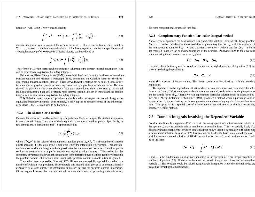
7.2 REMOVING DOMAIN INTEGRALS DUE TOINHOMOGENEOUSTERMS 119
Equation (7.2). Using Green’s second identityZ � r2v � vr2 � d = Z� � @v@n � v @ @n� d� (7.3)
domain integration can be avoided for certain forms of . If a v can be found which satisfiesr2v = !, where! is the fundamental solution of Laplace’s equation, then forthe specific case of being harmonic (r2 = 0) Green’s second identity can be reduced toZ ! d = Z� � @v@n � v @ @n� d� (7.4)
Therefore if a Galerkin vector can be found and is harmonic the domain integral in Equation (7.2)can be expressed as equivalent boundary integrals.
Fairweather, Rizzo, Shippy & Wu (1979) determined the Galerkin vector for the two-dimensionalPoisson equation and Monaco & Rangogni (1982) determined the Galerkin vector for the three-dimensional Poisson equation. Danson (1981) showed how this method can be applied successfullyfor a number of physical problems involving linear isotropic problems with body forces. He con-sidered the practical cases where the body force term arose due to either a constant gravitationalload, rotation about a fixed axis or steady-state thermal loading. In each of these cases the domainintegral can be expressed as equivalent boundary integrals.
This Galerkin vector approach provides a simple method of expressing domain integrals asequivalent boundary integrals. Unfortunately, it only applies to specific forms of the inhomoge-neous term (i.e., is required to be harmonic).
7.2.2 The Monte Carlo method
Domain discretisation could be avoided by using a Monte Carlo technique. This technique approx-imates a domain integral as a sum of the integrand at a number of random points. Specifically, intwo dimensions, a domain integralI is approximated asI � AN NXi=1 f (xi; yi) (7.5)
wheref (xi; yi) is the value of the integrand at random point(xi; yi), N is the number of randompoints used andA is the area of the region over which the integration is performed. This approxi-mation allows a domain integral to be approximated by a summation over a set of random pointsso domain integration can be performed without requiring a domain mesh. This method has thesecondary advantage of allowing the integration to be performed over a simple geometry enclosingthe problem domain - if a random point is not in the problem domain its contribution is ignored.
The method was proposed by Gipson (1987). Gipson has successfully applied this method to anumber of Poisson-type problems. Unfortunately this method often proves to be computationallyexpensive as a large number of integration points are neededfor accurate domain integration.Gipson argues however that, as this method removes the burden of preparing a domain mesh,
120 DOMAIN INTEGRALS IN THE BEM
the extra computational expense is justified.
7.2.3 Complementary Function-Particular Integral method
A more general approach can be developed using particular solutions. Consider the linear problemLu = . u can be considered as the sum of the complementary functionuc, which is a solution ofthe homogeneous equationLuc = 0, and a particular solutionup which satisfiesLup = but isnot required to satisfy the boundary conditions of the problem. Applying BEM to the governingequation using the expansionu = uc + up givesHu�Gq =Hup �Gqp (7.6)
If a particular solutionup can be found, all values on the right-hand-side of Equation (7.6) areknown - reducing the problem to Hu�Gq = d (7.7)
whered is a vector of known values. This linear system can be solved by applying boundaryconditions.
This approach can be applied in a situation where an analyticexpression for a particular solu-tion can be found. Unfortunately particular solutions are generally only known for simple operatorsand for simple forms of . Alternatively an approximate particular solution could be calculated nu-merically. Zheng, Coleman & Phan-Thien (1991) proposed a method where a particular solutionis determined by approximating the inhomogeneous source term using a global interpolation func-tion. This approach is a special case of a more general methodknown as the dual reciprocityboundary element method.
7.3 Domain Integrals Involving the Dependent Variable
Consider the linear homogeneous PDELu = 0. For many operators the fundamental solution tothe operatorL may be unobtainable or may be in an unusable form. This is especially likely if L
involves variable coefficients for which case it has been shown that it is particularly difficult to finda fundamental solution. Instead, a BEM formulation can be derived based on a related operator^L
with known fundamental solution. A BEM formulation forLu = 0 based on the operator^L willbe of the form Hu�Gq = � Z �^L� L� u! d (7.8)
where! is the fundamental solution corresponding to the operator^L. This integral equation issimilar to Equation (7.2). However in this case the domain integral term involves the dependentvariableu. This problem could be solved using domain integration where the internal nodes aretreated as formal problem unknowns.
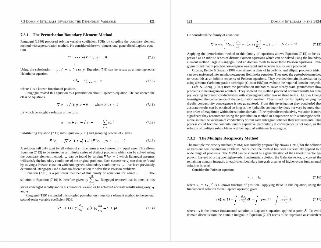
7.3 DOMAIN INTEGRALS INVOLVING THE DEPENDENT VARIABLE 121
7.3.1 The Perturbation Boundary Element Method
Rangogni (1986) proposed solving variable coefficient PDEsby coupling the boundary elementmethod with a perturbation method. He considered the two-dimensional generalised Laplace equa-tion r � (� (x; y)rV (x; y)) = 0 (7.9)
Using the substitutionV (x; y) = ��12u (x; y) Equation (7.9) can be recast as a heterogeneousHelmholtz equation r2u+ f (x; y)u = 0 (7.10)
wheref is a known function of position.Rangogni treated this equation as a perturbation about Laplace’s equation. He considered the
class of equations r2u+ "f (x; y)u = 0 where0 � " � 1 (7.11)
for which he sought a solution of the formu = u0 + "u1 + "2u2 + : : : = 1Xj=0 uj"j (7.12)
Substituting Equation (7.12) into Equation (7.11) and grouping powers of" givesr2u0 + " �r2u1 + fu0�+ "2 �r2u2 + fu1�+ : : : = 0 (7.13)
A solution will only exist for all values of" if the terms at each power of" equal zero. This allowsEquation (7.13) to be treated as an infinite series of distinct problems which can be solved usingthe boundary element method.u0 can be found by solvingr2u0 = 0 which Rangogni assumeswill satisfy the boundary conditions of the original problem. Each successiveuj can then be foundby solving a Poisson equation with homogeneous boundary conditions asuj�1 has been previouslydetermined. Rangogni used a domain discretisation to solvethese Poisson problems.
Equation (7.10) is a particular member of this family of equations for which" = 1. The
solution to Equation (7.10) is therefore given by
1Xj=0 uj. Rangogni reported that in practice this
series converged rapidly and in his numerical examples he achieved accurate results using onlyu0andu1.
Rangogni (1991) extended this coupled perturbation - boundary element method to the generalsecond-order variable coefficient PDEr2u+ f (x; y) @u@x + g (x; y) @u@y = h (x; y) (7.14)
122 DOMAIN INTEGRALS IN THE BEM
He considered the family of equationsr2u+ " �f (x; y) @u@x + g (x; y) @u@y � = h (x; y) (0 � " � 1) (7.15)
Applying the perturbation method to this family of equations allows Equation (7.15) to be ex-pressed as an infinite series of distinct Poisson equations which can be solved using the boundaryelement method. Again Rangogni used an domain mesh to solve these Poisson equations. Ran-gogni found that in practice convergence was rapid and accurate results were produced.
Gipson, Reible & Savant (1987) considered a class of hyperbolic and elliptic problems whichcan be transformed into an inhomogeneous Helmholtz equation. They used the perturbation methodto recast this as an infinite sequence of Poisson equations. They avoided domain discretisation byusing a Monte Carlo integration technique (Gipson 1987) to evaluate the required domain integrals.
Lafe & Cheng (1987) used the perturbation method to solve steady-state groundwater flowproblems in heterogeneous aquifers. They showed the methodproduced accurate results for sim-ply varying hydraulic conductivities with convergence after two or three terms. Lafe & Chenginvestigated the convergence of the perturbation method. They found that for rapidly varying hy-draulic conductivity convergence is not guaranteed. From this investigation they concluded thataccurate results can be obtained so long as the hydraulic conductivity does not vary by more thanone order of magnitude within the solution domain. If the hydraulic conductivity variation is moresignificant they recommend using the perturbation method inconjunction with a subregion tech-nique so that the variation of conductivity within each subregion satisfies their requirements. Thisprocess could become computationally expensive, particularly if convergence is not rapid, as thesolution of multiple subproblems will be required within each subregion.
7.3.2 The Multiple Reciprocity Method
The multiple reciprocity method (MRM) was initially proposed by Nowak (1987) for the solutionof transient heat conduction problems. Since then the method has been successfully applied to awide range of problems. The MRM can be viewed as a generalisation of the Galerkin vector ap-proach. Instead of using one higher-order fundamental solution, the Galerkin vector, to convert theremaining domain integrals to equivalent boundary integrals a series of higher-order fundamentalsolutions is used.
Consider the Poisson equation r2u = b0 (7.16)
whereb0 = b0 (x) is a known function of position. Applying BEM to this equation, using thefundamental solution to the Laplace operator, givesc (�) u (�) + Z� u@!0@n d� + Z b0!0 d = Z� !0 @u@n d� (7.17)
where!0 is the known fundamental solution to Laplace’s equation applied at point�. To avoiddomain discretisation the domain integral in Equation (7.17) needs to be expressed as equivalent
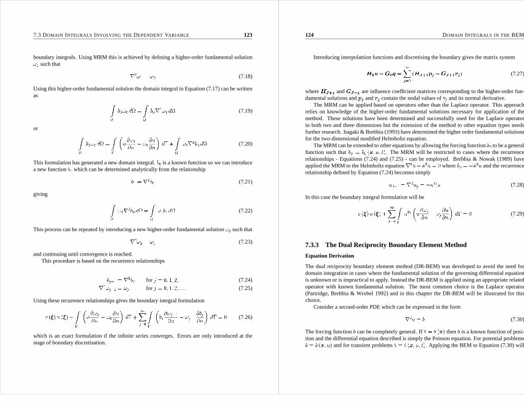
7.3 DOMAIN INTEGRALS INVOLVING THE DEPENDENT VARIABLE 123
boundary integrals. Using MRM this is achieved by defining a higher-order fundamental solution!1 such that r2!1 = !0 (7.18)
Using this higher-order fundamental solution the domain integral in Equation (7.17) can be writtenas Z b0!0 d = Z b0r2!1 d (7.19)
or Z b0!0 d = Z� �u@!1@n � !1@u@n� d� + Z !1r2b0 d (7.20)
This formulation has generated a new domain integral.b0 is a known function so we can introducea new functionb1 which can be determined analytically from the relationshipb1 = r2b0 (7.21)
giving Z !1r2b0 d = Z !1b1 d (7.22)
This process can be repeated by introducing a new higher-order fundamental solution!2 such thatr2!2 = !1 (7.23)
and continuing until convergence is reached.This procedure is based on the recurrence relationshipsbj+1 = r2bj for j = 0; 1; 2; : : : (7.24)r2!j+1 = !j for j = 0; 1; 2; : : : (7.25)
Using these recurrence relationships gives the boundary integral formulationc (�) u (�) + Z� �u@!0@n � !0@u@n� d� + 1Xj=0 Z� �bj @!j+1@n � !j+1@bj@n� d� = 0 (7.26)
which is an exact formulation if the infinite series converges. Errors are only introduced at thestage of boundary discretisation.
124 DOMAIN INTEGRALS IN THE BEM
Introducing interpolattion functions and discretising the boundary gives the matrix systemH0u�G0q = 1Xj=0 (HJ+1pj �GJ+1rj) (7.27)
whereHJ+1 andGJ+1 are influence coefficient matrices corresponding to the higher-order fun-damental solutions andpj andrj contain the nodal values ofbj and its normal derivative.
The MRM can be applied based on operators other than the Laplace operator. This approachrelies on knowledge of the higher-order fundamental solutions necessary for application of themethod. These solutions have been determined and successfully used for the Laplace operatorin both two and three dimensions but the extension of the method to other equation types needsfurther research. Itagaki & Brebbia (1993) have determinedthe higher order fundamental solutionsfor the two-dimensional modified Helmholtz equation.
The MRM can be extended to other equations by allowing the forcing functionb0 to be a generalfunction such thatb0 = b0 (x; u; t). The MRM will be restricted to cases where the recurrencerelationships - Equations (7.24) and (7.25) - can be employed. Brebbia & Nowak (1989) haveapplied the MRM to the Helmholtz equationr2u+ �2u = 0 whereb0 = ��2u and the recurrencerelationship defined by Equation (7.24) becomes simplyuj+1 = r2uj = ��2ju (7.28)
In this case the boundary integral formulation will bec (�) u (�) + 1Xj=0 Z� �2j �u@!j@n � !j @u@n� d� = 0 (7.29)
7.3.3 The Dual Reciprocity Boundary Element Method
Equation Derivation
The dual reciprocity boundary element method (DR-BEM) was developed to avoid the need fordomain integration in cases where the fundamental solutionof the governing differential equationis unknown or is impractical to apply. Instead the DR-BEM is applied using an appropriate relatedoperator with known fundamental solution. The most common choice is the Laplace operator(Partridge, Brebbia & Wrobel 1992) and in this chapter the DR-BEM will be illustrated for thischoice.
Consider a second-order PDE which can be expressed in the formr2u = b (7.30)
The forcing functionb can be completely general. Ifb = b (x) thenb is a known function of posi-tion and the differential equation described is simply the Poisson equation. For potential problemsb = b (x; u) and for transient problemsb = b (x; u; t). Applying the BEM to Equation (7.30) will

7.3 DOMAIN INTEGRALS INVOLVING THE DEPENDENT VARIABLE 125
give Hu�Gq = � Z b! d (7.31)
where! is the known fundamental solution to Laplace’s equation. The aim of the DR-BEM is toexpress the domain integral due to the forcing functionb as equivalent boundary integrals.
The DR-BEM uses the idea of approximatingb using interpolation functions. A global approx-imation tob of the form b = MXj=1 �jfj (7.32)
is proposed.�j are unknown coefficients andfj are approximating functions used in the interpo-lation and are generally chosen to be functions of the sourcepoint and the field point of the fun-damental solution. The approximating functionsfj are applied atM different collocation points- called poles - generally most, but not all, of which are located on the boundary of the problemdomain.
As discussed in the previous chapter the solution to a linearPDELu = can be constructed asthe sum of a complimentary functionuc (which satisfies the homogeneous equationLuc = 0) and aparticular solutionup to the equationLup = . Instead of using a single particular solution, whichmay be difficult to determine, the DR-BEM employs a series of particular solutions^uj which arerelated to the approximating functionsfj as shown in Equation (7.33).r2^uj = fj j = 1; : : : ;M (7.33)
By substituting Equations (7.32) and (7.33) into Equation (7.30) the forcing functionb is approxi-mated by a weighted summation of particular solutions to thePoisson equation.r2u = MXj=1 �jr2^uj (7.34)
The DR-BEM essentially constructs an approximate particular solution to the governing PDE as asummation of localised particular solutions.
With the governing equation rewritten in the form of Equation (7.34) the standard boundaryelement approach can be applied. Equation (7.34) is multiplied by a weighting function! andintegrated over the domain. Green’s theorem is applied twice and the fundamental solution of theLaplacian is used to remove the remaining domain integrals.The name dual reciprocity BEM isderived from the application of reciprocity relationshipsto both sides of Equation (7.34). Afterapplying these steps Equation (7.35) is obtained, where thefundamental solution pole is applied at
126 DOMAIN INTEGRALS IN THE BEM
point�.c (�)u (�) + Z� �u@!@n � !@u@n� d�= MXj=1 �j0@c (�)uj (�) + Z� �^uj @!@n � !@hatuj@n � d�1A (7.35)
In implementing a numerical solution of this equation similar steps are taken as for the standardBEM. The boundary is discretised into elements and interpolation functions are introduced to ap-proximate the dependent variable within each element.
The form of each^uj is known from Equation (7.33) once the approximating functionsfj havebeen defined. It is not necessary to use interpolation functions to approximate each^uj. Howeverby using the same interpolation functions to approximateu and^uj the numerical implementationwill generate the same matricesH andG on both sides of Equation (7.35). The error generatedby approximating each^uj in this manner has been found to be small and can be justified bytheimproved computational efficiency of the method (Partridgeet al. 1992).
The application of this method results in the systemHu�Gq = N+IXj=1 �j (H ^uj �G^qj) (7.36)
where theM poles were chosen to be theN boundary nodes plusI internal points so thatM =N + I. Although it is not generally necessary to include poles at internal points it has been foundthat in general improved accuracy is achieved by doing so (Nowak & Partridge 1992). It hasbeen shown that for many problems (Partridge et al. 1992) (Huang & Cruse 1993) using boundarypoints only in this procedure is insufficient to define the problem. In general using internal pointsis likely to improve the solution accuracy as it increases the number of degrees of freedom. Notheory has been developed of how many internal collocation points should be used for optimalaccuracy, or where these points should be positioned withinthe problem domain. Using internalpoles in this interpolation does not require domain discretisation - it is only necessary to specifythe coordinates of the internal collocation points. The internal points can be chosen to be locationswhere the solution is of interest.
The ^uj and ^qj vectors can be treated as columns of the matrices^U and ^Q respectively. Thisallows Equation (7.36) to be rewritten asHu�Gq = �H ^U �G ^Q�� (7.37)
where� is a vector containing the nodal values of�. To solve this system it is necessary to evaluate�. � is defined by Equation (7.32) which, for the nodal values, canbe expressed in matrix form asb = F�. If theF matrix is nonsingular this expression can be rearranged to give Equation (7.38)which provides an explicit expression for�.� = F�1b (7.38)

7.3 DOMAIN INTEGRALS INVOLVING THE DEPENDENT VARIABLE 127
Including this explicit expression for� in Equation (7.37) givesHu�Gq = �H ^U �G ^Q�F�1b (7.39)
The approach taken to solve this equation will depend on the form of b.The Approximating Function f
The accuracy of the DR-BEM hinges on the accuracy of the global approximation to the forcingfunctionb (defined by Equation (7.32)). Therefore the choice of the approximating functionsfj isa key consideration when implementing the DR-BEM. The only requirement so far prescribed onthe form of the approximating functionsfj is that theF matrix generated should be nonsingularand that the related particular solutions^uj can be determined and can be expressed in a practicalclosed form. Some work has been conducted into investigating what form offj should be used ina given situation to provide the highest accuracy and computational efficiency.
Usually a form offj is defined and this can be used, applying Equation (7.33), to specify ^u
and^q. The fundamental solution of Laplace’s equation is! (x; �) = � 12� ln r in two-dimensional
space and! (x; �) = 14�r in three-dimensional space - wherer is the Euclidean distance between
the field pointx and the source point� of the fundamental solution. Due to the dependence of thisfundamental solution only onr the approximating function is generally chosen to be some radialfunction i.e.,fj = fj (r). Several other options forfj have been tried (Partridge et al. 1992) but ithas been found that in general the most accurate results weregenerated using some radial function.For both two and three-dimensional problems Wrobel, Brebbia & Nardini (1986) recommendedchoosingfj from the series fj = 1 + rj + r2j + : : :+ rmj (7.40)
whererj is the distance between the field point (nodej) and the DR-BEM collocation point (nodei). They showed that accurate results can be achieved using some combination of terms from thisseries. Generally the same approximating functionfj is used at all the collocation points so in thisthesis, for simplicity, the form of approximating functionsfj will be referred to by a singlef .
Choosingf to be a function of only one variable simplifies the process ofdetermining^u and^q.For two-dimensional problems, iff = f (r) then the relationshipr2^u = f (r) (7.41)
can be reduced to the ordinary differential equationd2^udr2 + 1r d^udr = f (7.42)
Using f defined by Equation (7.40) the corresponding forms of^u and ^q, for two-dimensional
128 DOMAIN INTEGRALS IN THE BEM
problems, can be shown to be^u = r24 + r39 + : : :+ rm+2(m + 2)2 (7.43)^q = �rx@x@n + ry @y@n��12 + r3 + : : :+ rmm+ 2� (7.44)
whererx = xj � xi andry = yj � yi.Any combination of terms from Equation (7.40) can be used forspecifyingf . It has been found
that in general including higher-order terms leads to little improvement in accuracy (Partridgeet al. 1992). The most commonly used form isf = 1+ r as this approximation will generally giveaccurate results with greater computational efficiency than other choices.
Equation (7.40) was recommended as a basis for the approximating function f due to theparticular form of the fundamental solution of Laplace’s equation and its dependence onr only. Ifa different operator is used as the basis of the DR-BEM then itis likely a different form off willbe more appropriate. The choice off in this case will be discussed in Section 7.3.3.
The performance of the DR-BEM hinges on the choice of the approximating functionf . Thetheory of how to determine the best approximating function is therefore a vital component ofthe DR-BEM. Unfortunately the approximating function has generally been chosen and used in arather ad-hoc manner. Recently some more formal analysis ofthe use of approximating functionshas been undertaken.
Golberg & Chen (1994) argued that a formal analysis of the approximating functionf can beundertaken using the theory of radial basis functions. Radial basis functions are a generalisationof cubic splines in multi-dimensions. Cubic splines are known to be optimal for one-dimensionalinterpolation. Therefore, rather than being an arbitrary choice, it seems that choosingf to bea radial function is a logical extension for two or three-dimensional problems. Golberg & Chenshowed that, for the Poisson equation, choosingf to be a radial basis function ensures convergenceof the DR-BEM.
They also demonstrated thatf = 1 + r is a specific member of the group of radial basisfunctions. The theory of using radial basis functions for multi-dimensional approximation is fairlyadvanced. It has been shown thatf = r is optimal for three-dimensional problems which justifiesthe use off = 1 + r when applying the DR-BEM to three-dimensional problems - the constantis included to ensure a non-zero diagonal forF . However for two-dimensional problems it hasbeen shown that optimal approximation is attained using thethin plate splinef = r2logr. Thisobservation lead Golberg & Chen to suggest that choosingf to be a thin plate spline may improvethe accuracy of the DR-BEM in two dimensions. Recently Golberg (1995) has published a reviewof the DR-BEM concentrating on developments since 1990 concerning the numerical evaluationof particular solutions.
Inhomogeneous Equations
If the forcing functionb is a function of position only then the differential equation under consid-eration is simply Poisson’s equation. In this case it is not necessary to invert theF matrix as� cansimply be calculated fromb = F� using Gaussian elimination. Equation (7.39) can be rewritten

7.3 DOMAIN INTEGRALS INVOLVING THE DEPENDENT VARIABLE 129
as Hu�Gq = d whered = �H ^U �G ^Q�� (7.45)
By applying boundary conditions Equation (7.45) can be reduced to a linear systemAx = �
which can be solved to give the unknown nodal values ofu andq.Zheng et al. (1991) and Coleman, Tullock & Phan-Thien (1991)have proposed a method which
uses a global shape function to construct an approximate particular solution. As discussed byPolyzos, Dassios & Beskos (1994) this method is essentiallyequivalent to the DR-BEM. However,Zheng et al. and Coleman et al. suggested several alternative ways of determining the unknowncoefficients�j for inhomogeneous equations. Zheng et al. (1991) used a least-squares methodwhere they minimised the sum of squaresS = MXm=1 b (rm)� NXj=1 �jfj (rm)! (7.46)
using singular value decomposition. For large systems theyfound the computational efficiencycould be improved by employing the conjugate gradient method. Coleman et al. (1991) success-fully solved inhomogeneous potential and elasticity problems which are governed by operatorsother than the Laplacian.
Elliptic Problems
If b is a function of the dependent variable then� will also be a function of the dependent variable.Consider, for example, the linear second-order differential equationr2u+ u = 0 (7.47)
In this caseb = �u so� = F�1�u. Applying the DR-BEM to Equation (7.47), based on thefundamental solution to Laplace’s equation, givesHu�Gq = ��H ^U �G ^Q�F�1u (7.48)
which can be rearranged to give(H + S)u = Gq whereS = �H ^U �G ^Q�F�1 (7.49)
Again, by applying boundary conditions Equation (7.49) canbe reduced to a linear systemAX =� which can be solved to determine the unknown nodal values.Due to the presence of the fully-populatedF�1 matrix in Equation (7.49) it is not possible to
solve the boundary problem and internal problem separately. Instead the solution can be treated asa coupled problem and the solutions at boundary and internalnodes are generated simultaneously.
Derivative Terms The DR-BEM can also be applied for elliptic problems whereb involvesderivatives of the dependent variable (Partridge et al. 1992). Consider, for example, the differ-
130 DOMAIN INTEGRALS IN THE BEM
ential equation r2u+ @u@x = 0 (7.50)
In this case applying DR-BEM, using the Laplace fundamentalsolution, givesHu�Gq = ��H ^U �G ^Q�F�1@u@x (7.51)
To solve this problem it is necessary to relate the nodal values ofu to the nodal values of
@u@x . This
is achieved by using interpolation functions to approximateu in a similar manner as was used toapproximateb in Equation (7.32). A global approximation function of the formu = MXj=1 �j (x; y)�j (7.52)
can be used to approximateu where�j are the chosen interpolation functions and�j are the un-known coefficients. In system form this can be expressed asu = �� (7.53)
Although it is not necessary, equating� toF improves the computational efficiency of the methodas only one matrix inversion procedure is required. Differentiating Equation (7.53) gives@u@x = @�@X� (7.54)
Choosing� = F and inverting Equation (7.53) to give an explicit expression for � allows Equa-tion (7.54) to be rewritten as @u@x = @F@XF�1u (7.55)
Equation (7.39) can now be rewritten as(H +R)u = Gq whereR = �H ^U �G ^Q�F�1 @F@XF�1 (7.56)
By applying boundary conditions Equation (7.56) can be reduced to a linear system which can besolved to give the unknown nodal values.
As mentioned earlier, the approximating functionf is generally chosen to bef = 1 + r. Thiscan lead to numerical problems if derivative terms are included in the forcing functionb. As shownin Equation (7.55) derivative terms require derivatives off to be evaluated. For example, evaluating

7.3 DOMAIN INTEGRALS INVOLVING THE DEPENDENT VARIABLE 131
the
@F@X matrix requires calculation of
@f@x . Using the approximating functionf = 1 + r gives@f@x = @f@r @r@x = @f@r rxr (7.57)
This derivative function can become singular, so - as shown by Zhang (1993) - significant numericalerror may result. This will especially be the case in problems where collocation points are locatedclose together.
Zhang (1993) suggested two possibilities for avoiding thisproblem. The first suggestion in-volved using a mapping procedure to map the governing equation to an equation without convec-tive terms. This method was shown to produce accurate results but is somewhat cumbersome andcan only be applied to linear problems. A simpler approach isto choose an approximating func-tion which does not lead to singularities for convective terms. Zhang recommended use of eitherf = 1+ r3 or f = 1+ r2+ r3. These approximating functions produce accurate results and can besimply applied for both linear and nonlinear problems. Zhang recommended the adoption of theseapproximating functions for all use of the DR-BEM.
The same idea of using Equation (7.53) to allow nodal values of u to be associated to itsderivatives can be applied to extend the DR-BEM to cases involving higher-order derivatives orcross derivatives of the dependent variable. Appropriate approximating functions need to be chosento avoid the problem of singularities.
Variable Coefficients The DR-BEM can be readily extended to equations with variable coeffi-cients. Consider the variable coefficient Helmholtz equationr2u+ � (x) u = 0 (7.58)
where� is a function of position -� = � (x; y) in two dimensions. If the DR-BEM is applied usingthe known fundamental solution to the Laplace operator thenthe forcing function isb = ��u.Applying the DR-BEM givesHu�Gq = �H ^U �G ^Q�F�1b (7.59)
whereb is a vector of the nodal values of the forcing functionb. The relationshipb = ��u can bewritten in matrix form asb = �Ku whereK is a diagonal matrix containing the nodal values of� (x; y) i.e., K = 26664� (x1; y1) 0 � � � 00 � (x2; y2) � � � 0
......
. . ....0 0 � � � � (xM ; yM)37775 (7.60)
whereM is the number of collocation points used in applying the DR-BEM.
132 DOMAIN INTEGRALS IN THE BEM
Using this matrix expression forb Equation (7.59) can be rearranged to give(H + SK)u = Gq whereS = �H ^U �G ^Q�F�1 (7.61)
which is a boundary-only expression for the variable coefficient Helmholtz equation. This methodis general and can easily be extended to accommodate variable coefficient derivative terms and asum of variable coefficient terms.
Formulating the DR-BEM for a General Elliptic Problem In this section it has been shownhow the DR-BEM can be applied for elliptic problems with varying forms ofb. The DR-BEM canbe applied in cases whereb involves a sum of terms due to the basic propertyZ (b1 + b2) d = Z b1 d + Z b2 d (7.62)
Consider a two-dimensional equation of the formr2u (x; y) = k (x; y)u+ l (x; y) @u@x +m (x; y) @u@y + n (x; y) (7.63)
Applying the DR-BEM to this equation gives a matrix system ofthe form(H �R)u = Gq + Sn (7.64)
where S = �H ^U �G ^Q�F�1 (7.65)R = S �K + �L@F@X +M@F@Y �F�1� (7.66)K, L andM are diagonal matrices where the diagonals contain the nodalvalues ofk, l andm
respectively.n is a vector containing the nodal values ofn.
The DR-BEM Using Other Operators
The DR-BEM has been presented in this chapter based on the Laplace operator. However the DR-BEM can be be applied using essentially any operator of appropriate order with known fundamentalsolution. If an appropriate operator can be found the complexity of the forcing functionb can bereduced. This should improve the accuracy of the method. Theproblem with applying the DR-BEM based on another operator is in choosing the approximating functionf . A choice off whichproduces accurate results is required but it is also necessary to choose anf for which a particularsolution^u can be determined.
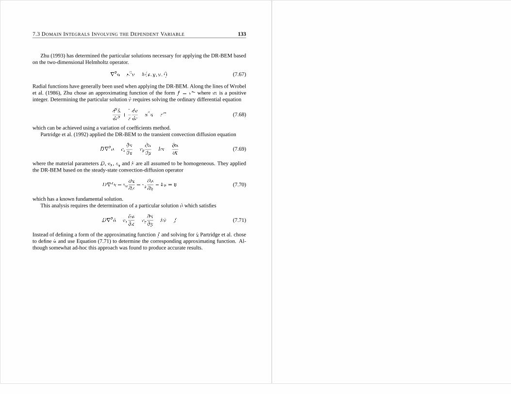
7.3 DOMAIN INTEGRALS INVOLVING THE DEPENDENT VARIABLE 133
Zhu (1993) has determined the particular solutions necessary for applying the DR-BEM basedon the two-dimensional Helmholtz operator.r2u+ �2u = b (x; y; u; t) (7.67)
Radial functions have generally been used when applying theDR-BEM. Along the lines of Wrobelet al. (1986), Zhu chose an approximating function of the form f = rm wherem is a positiveinteger. Determining the particular solution^u requires solving the ordinary differential equationd2^udr2 + 1r d^udr + �2u = rm (7.68)
which can be achieved using a variation of coefficients method.Partridge et al. (1992) applied the DR-BEM to the transient convection diffusion equationDr2u� vx@u@x � vy @u@y � ku = @u@t (7.69)
where the material parametersD, vx, vy andk are all assumed to be homogeneous. They appliedthe DR-BEM based on the steady-state convection-diffusionoperatorDr2u� vx@u@x � vy @u@y � ku = 0 (7.70)
which has a known fundamental solution.This analysis requires the determination of a particular solution ^u which satisfiesDr2^u� vx@^u@x � vy @^u@y � k^u = f (7.71)
Instead of defining a form of the approximating functionf and solving for^u Partridge et al. choseto define^u and use Equation (7.71) to determine the corresponding approximating function. Al-though somewhat ad-hoc this approach was found to produce accurate results.

Chapter 8
The BEM for Parabolic PDES
8.1 Time-Stepping Methods
Several approaches have been proposed for applying the BEM to parabolic problems. These meth-ods can be broadly classified into two main approaches. Either some form of time-stepping proce-dure is used to advance the solution in time, or a semi-analytic technique is used which can directlycalculate a solution at a specified time. In this section time-stepping procedures will be considered.
Time-stepping approaches discretise the time domain in some manner and use some form oftime marching scheme to advance the solution from one discrete time to the next. The two mostcommonly used time-stepping methods are the coupled finite difference - BEM and the direct timeintegration method. These two methods will be outlined in this section for the diffusion equationr2u (x; t) = 1� @u (x; t)@t (8.1)
where the diffusivity� is a material parameter which can be a constant or a function of position.
8.1.1 Coupled Finite Difference - Boundary Element Method
This approach discretises the time-domain in a finite difference form. Consider the variation be-tween a timetm and a timetm+1 = tm+�t. The most common approach (Brebbia et al. 1984b) isto assume that, for sufficiently small�t, the time derivative can be approximated using a first-orderfully implicit finite difference scheme@u (x; tm+1)@t = u (x; tm+1)� u (x; tm)�t (8.2)
which allows the diffusion equation in this time-range to beapproximated asr2u �x; tm+1�� 1��tu �x; tm+1�+ 1��tu (x; tm) = 0 (8.3)
Using this finite difference approximation the original parabolic equation has been reduced to anelliptic equation. Using the weighted residuals method an integral equation can be generated from
136 THE BEM FOR PARABOLIC PDES
Equation (8.3). c (�)um+1 + Z� um+1@!@n d� = Z qm+1!d� + 1��t Z um! d (8.4)
whereum+1 = u (x; tm+1) andum = u (x; tm). The fundamental solution! is a solution of themodified Helmholtz equationr2! (x; �)� 1��t! (x; �) + � (�) = 0 (8.5)
applied at some source point�. The fundamental solution of the modified Helmholtz equationis known in both two and three dimensions. If an internal solution is required at a specific timethis can be determined explicitly from Equation (8.4) wherethe fundamental solution is applied atinternal point� andc (�) = 1.
Unfortunately Equation (8.4) contains a domain integral. This integral is generally evaluated byusing a domain mesh (Brebbia et al. 1984b). The domain integral does not include any problem un-knowns so a fairly coarse domain mesh will generally suffice.Applying the BEM to Equation (8.4)gives Hum+1 �Gqm+1 = Bum (8.6)
whereB is a matrix containing the influence coefficients due to the domain integral. Using Equa-tion (8.6) the solution can be advanced in time.U0 is known from the initial conditions so asolution can be calculated att = t0 +�t. A solution at internal nodes can then be calculated. Thetime-stepping procedure can be repeated using the internalsolution att = t0+�t as pseudo-initialconditions for the next time-step.
If a constant time-step is used the matricesH, G andB can be calculated once and stored.The boundary conditions can be applied to form a solution system of the formAxm+1 = � wherexm+1 is the vector of unknown nodal values at timetm+1 and � is a vector constructed fromknown nodal values from the previous time-step. For a problem with time-independent boundaryconditions at each time-step it is only necessary to update� and solve the system forxm+1. If aproblem has time-dependent boundary conditions the solution system needs to be reformed at eachtime-step.
This coupled finite difference - boundary element method (FD-BEM) was first proposed byBrebbia & Walker (1980) for the diffusion equation. It was implemented and investigated byCurran, Cross & Lewis (1980). They found that this method will only produce accurate resultsif Equation (8.2) accurately approximates the time derivative. This will generally require smalltime-steps to be adopted. Curran et al. investigated the useof a higher-order approximation to thetime-derivative. They found that this improved the accuracy of the method. Unfortunately it leadto a deterioration in convergence behaviour.
Tanaka, Matsimoto & Yang (1994) proposed a generalised version of this time-stepping scheme.They approximated the time variation within an interval asu (x; t) = �u �x; tm+1�+ (1� �) u (x; tm) (8.7)

8.1 TIME-STEPPING METHODS 137
where�, termed the time-scheme parameter, is a constant in the range 0 < � � 1. Substitutingthis approximation and a first-order finite difference approximation of the time derivative into thediffusion equation gives �r2um+1 + (1� �)r2um = um+1 � um��t (8.8)
If � = 1 this approximation of the diffusion equation is equivalentto the standard FD-BEM dis-cussed earlier. An integral equation can be derived from Equation (8.8). Tanaka et al. implementedthis method and found it gave accurate results for a range of diffusion problems. They tested theaccuracy for a Crank-Nicolson scheme (� = 12 ), a Galerkin scheme (� = 23 ) and a fully implicitscheme (� = 1). They found that the best results were achieved using a Crank-Nicolson scheme.
8.1.2 Direct Time-Integration Method
Instead of converting the original parabolic equation to anelliptic equation the problem can betreated directly in the time domain by directly integratingover both time and space. The weightedresidual statement using this approach istFZt0 Z �r2u (x; t)� 1� @u (x; t)@t �! (�;x; tF ; t) d dt = 0 (8.9)
Integrating in time once and in space twice givesc (�)u (�; tF ) + � tFZt0 Z� u@!@n d� dt = � tFZt0 Z� q! d� dt+ Z u (x; t0)! d (8.10)
where the fundamental solution! satisfies�r2! (�;x; tF ; t) + @! (�;x; tF ; t)@t + � (�) � (tF ) = 0 (8.11)
This time dependent fundamental solution is known in two andthree dimensions. Physically thisfundamental solution represents the effect at a field pointx at timet of a unit point source appliedat a point� at timetF . If an internal solution is required at a specific time this can be determinedfrom Equation (8.10) withc (�) = 1.
The variation ofu andq with time is unknown so it is still necessary to step in time. However,as the time dependence is included in the fundamental solution, accurate results can be achievedusing larger time-steps than with the FD-BEM. Two differenttime-stepping schemes can be used.Similarly to the FD-BEM, each time-step can be treated as a new problem so that an internalsolution is constructed at the end of each time-step to be used as pseudo-initial conditions for thenext time-step. Alternatively the time integration process can be restarted att0 with increasingnumbers of intermediate steps used. These two time-stepping approaches are discussed in detail inBrebbia et al. (1984b).
The first method requires a new domain integral to be calculated after each time-step due to
138 THE BEM FOR PARABOLIC PDES
the updated pseudo-initial conditions. The second time-stepping procedure involves only a domainintegral att0 so, ideally, a domain integral only needs to be calculated once. This, however, will stillrequire the user to create a domain mesh. As mentioned by Brebbia et al. (1984b), in many practicalcases the domain integral can be avoided. If the initial conditions areu0 = 0 throughout the bodythe domain integral equals zero. If the initial conditions satisfy Laplace’s equationr2u0 = 0 thena Galerkin vector can be found and the domain integral can be expressed as equivalent boundaryintegrals. This includes many practical cases such as constant initial temperature or an initial lineartemperature profile.
Unfortunately, in practice it is not always feasible to restart the integration process att0. Ateach time-step newH andG matrices are required so if many time-steps are required thestoragecapacity of the computer is likely to be exceeded. This requires the procedure to be restartedat some time where an internal solution is constructed and used as pseudo-initial conditions torepeat the process. Therefore, in practice, both time-stepping methods are likely to require domainintegration.
8.2 Laplace Transform Method
An alternative approach which avoids time-stepping is to solve the problem in a transform domainwhich removes the time dependence of the problem. The parabolic PDE is thus converted to anelliptic problem for which the boundary element method has been shown to generally produceaccurate results. Once the solution to the elliptic problemis determined in the transform spacea solution in the original space can be attained using an inverse transform procedure. The mostappropriate transform approach for parabolic problems is the Laplace transform.
Consider the diffusion equationr2u (x; t) = 1� @u (x; t)@t (8.12)
with appropriate boundary and initial conditions. The Laplace transform ofu (x; t) will be sym-bolised asU (x; �) and is defined asU (x; �) = 1Z0 e��tu (x; t) dt (8.13)
Applying Laplace transforms to Equation (8.12) givesr2U (x; �) = 1� (�U (x; �)� u0 (x)) (8.14)
with transformed boundary conditions.u0 (x) is the initial conditions ofu. Equation (8.14) is anelliptic PDE which can be readily solved using the boundary element method. Once the solutionis determined in Laplace transform space this solution can be inverted to give a solution in thetime-domain. This inversion procedure requires solutionsto be generated for several values of thetransform parameter�.
This method was first proposed by Rizzo & Shippy (1970) and hassince been successfully
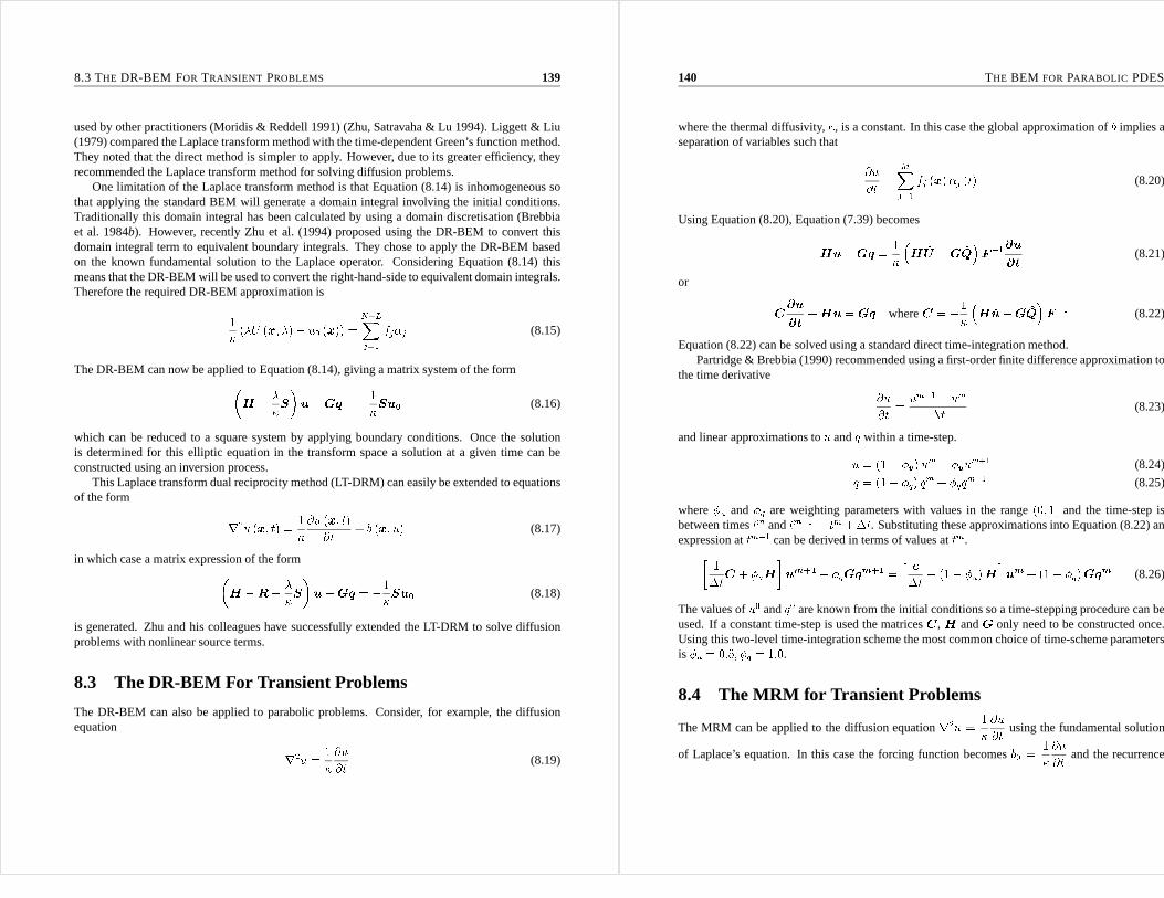
8.3 THE DR-BEM FOR TRANSIENT PROBLEMS 139
used by other practitioners (Moridis & Reddell 1991) (Zhu, Satravaha & Lu 1994). Liggett & Liu(1979) compared the Laplace transform method with the time-dependent Green’s function method.They noted that the direct method is simpler to apply. However, due to its greater efficiency, theyrecommended the Laplace transform method for solving diffusion problems.
One limitation of the Laplace transform method is that Equation (8.14) is inhomogeneous sothat applying the standard BEM will generate a domain integral involving the initial conditions.Traditionally this domain integral has been calculated by using a domain discretisation (Brebbiaet al. 1984b). However, recently Zhu et al. (1994) proposed using the DR-BEM to convert thisdomain integral term to equivalent boundary integrals. They chose to apply the DR-BEM basedon the known fundamental solution to the Laplace operator. Considering Equation (8.14) thismeans that the DR-BEM will be used to convert the right-hand-side to equivalent domain integrals.Therefore the required DR-BEM approximation is1� (�U (x; �)� u0 (x)) = N+LXj=1 fj�j (8.15)
The DR-BEM can now be applied to Equation (8.14), giving a matrix system of the form�H � ��S�u�Gq = �1�Su0 (8.16)
which can be reduced to a square system by applying boundary conditions. Once the solutionis determined for this elliptic equation in the transform space a solution at a given time can beconstructed using an inversion process.
This Laplace transform dual reciprocity method (LT-DRM) can easily be extended to equationsof the form r2u (x; t) = 1� @u (x; t)@t + b (x; u) (8.17)
in which case a matrix expression of the form�H �R� ��S�u�Gq = �1�Su0 (8.18)
is generated. Zhu and his colleagues have successfully extended the LT-DRM to solve diffusionproblems with nonlinear source terms.
8.3 The DR-BEM For Transient Problems
The DR-BEM can also be applied to parabolic problems. Consider, for example, the diffusionequation r2u = 1� @u@t (8.19)
140 THE BEM FOR PARABOLIC PDES
where the thermal diffusivity,�, is a constant. In this case the global approximation ofb implies aseparation of variables such that @u@t = MXj=1 fj (x)�j (t) (8.20)
Using Equation (8.20), Equation (7.39) becomesHu�Gq = 1� �H ^U �G ^Q�F�1@u@t (8.21)
or C@u@t +Hu = Gq whereC = �1� �H ^u�G ^Q�F�1 (8.22)
Equation (8.22) can be solved using a standard direct time-integration method.Partridge & Brebbia (1990) recommended using a first-order finite difference approximation to
the time derivative @u@t = um+1 � um�t (8.23)
and linear approximations tou andq within a time-step.u = (1� �u) um + �uum+1 (8.24)q = (1� �q) qm + �qqm+1 (8.25)
where�u and�q are weighting parameters with values in the range(0; 1] and the time-step isbetween timestm andtm+1 = tm +�t. Substituting these approximations into Equation (8.22) anexpression attm+1 can be derived in terms of values attm.� 1�tC + �uH�um+1 � �qGqm+1 = h c�t � (1� �u)Hium + (1� �q)Gqm (8.26)
The values ofu0 andq0 are known from the initial conditions so a time-stepping procedure can beused. If a constant time-step is used the matricesC, H andG only need to be constructed once.Using this two-level time-integration scheme the most common choice of time-scheme parametersis �u = 0:5; �q = 1:0.
8.4 The MRM for Transient Problems
The MRM can be applied to the diffusion equationr2u = 1� @u@t using the fundamental solution
of Laplace’s equation. In this case the forcing function becomesb0 = 1� @u@t and the recurrence

8.4 THE MRM FOR TRANSIENT PROBLEMS 141
relationship defined by Equation (7.24) becomesuj+1 = r2uj = @ju@tj (8.27)
The higher-order fundamental solutions are known for Laplace’s equation. In this case the MRMformulation becomes c (�)u (�) + 1Xj=0 Z� @!@n @ju@tj d� = 1Xj=0 Z� !@jq@tj d� (8.28)
The standard BEM numerical procedure can be applied to this boundary integral equation. Thisgives the matrix systemH0u+H1 _u+H2�u+ : : : = G0q +G1 _q +G2�q + : : : (8.29)
where the matricesH1;G1 etc are the influence coefficient matrices relating to the higher-orderfundamental solutions. This equation can be solved using a time-integration procedure.
The most common approach is to solve this system numericallyby discretising the time domainand using a time-stepping procedure. This requires some interpolation between the two time-levelsmarked bym andm+ 1. This most common approach is to use a linear approximation to u andq
in this time-range u = (1� �) um + �um+1 (8.30)q = (1� �) qm + �qm+1 (8.31)
where� has a value in the range 0 to 1. Differentiating these linear approximations gives_u = um+1 � um�tm (8.32)_q = qm+1 � qm�tm (8.33)
and all the other derivatives vanish.This allows Equation (8.29) to be simplified toHLum+1 �GLqm+1 = �HRum +GRqm (8.34)
whereHL = 1�tmH1 + �H0, HR = � 1�tmH1 + (1� �)H0, GL = 1�tmG1 + �G0, GR =� 1�tmG1 + (1� �)G0. This approach is termed a first-order approach as it removesall but the
first derivatives. A second order approach can be formulatedby using quadratic interpolation ofuandq within the time-range.
Using Equation (8.34) the solution can be advanced in time. If a constant time-step is used thematricesHL;HR;GL andGR only need to be constructed once outside the time-stepping loop.If the boundary conditions are not time-dependent the boundary conditions only need to be applied
142 THE BEM FOR PARABOLIC PDES
once.

Bibliography
Brebbia, C. A. & Nowak, A. (1989), A new approach for transforming domain integrals to theboundary,in R. Gruber, J. Periaux & R. P. Shaw, eds, ’Proceedings of the Fifth InternationalSymposium on Numerical Methods in Engineering’, Computational Mechanics Publications,Springer-Verlag, pp. 73–84.
Brebbia, C. A., Telles, J. C. F. & Wrobel, L. C. (1984a), Boundary Element Techniques, Springer-Verlag.
Brebbia, C. A., Telles, J. C. F. & Wrobel, L. C. (1984b), Boundary element techniques: Theoryand applications in engineering, Springer-Verlag, New York.
Brebbia, C. A. & Walker, S. (1980),Boundary Element Techniques In Engineering, Newnes–Butterworths.
Clements, D. L. & Rizzo, F. (1978), ’A method for the numerical solution of boundary valueproblems governed by second-order elliptic systems’,Journal of the Institute of MathematicsApplications22, 197–202.
Coleman, C. J., Tullock, D. L. & Phan-Thien, N. (1991), ’An effective boundary element methodfor inhomogeneous partial differential equations’,Journal of Applied Mathematics andPhysics (ZAMP)42, 730–745.
Curran, D. A. S., Cross, M. & Lewis, B. A. (1980), ’Solution ofparabolic differential equations bythe boundary element method using discretisation in time’,Applied Mathematical Modelling4, 398–400.
Danson, D. J. (1981), A boundary element formulation of problems in linear isotropic elasticitywith body forces,in C. A. Brebbia, ed., ’Boundary Element Methods’, Computational Me-chanics Publications and Springer-Verlag, pp. 105–122.
Fairweather, G., Rizzo, F. J., Shippy, D. J. & Wu, Y. S. (1979), ’On the numerical solution oftwo-dimensional problems by an improved boundary integralequation method’,J. Comput.Phys.31, 96–112.
Gipson, G. S. (1987),Boundary Element Fundamentals - Basic Concepts And Recent Develop-ments In The Poisson Equation, Computational Mechanics Publications.
Gipson, G. S., Reible, D. D. & Savant, S. A. (1987), Boundary elements and perturbation theoryfor certain classes of hyperbolic and parabolic problems,in C. A. Brebbia, W. L. Wendland &
144 BIBLIOGRAPHY
G. Kuhn, eds, ’Boundary Elements IX’, Computational Mechanics Publications and Springer-Verlag, pp. 115–127.
Golberg, M. A. (1995), ’The numerical evaluation of particular solutions in the BEM - a review’,Boundary Element Communications.
Golberg, M. A. & Chen, C. S. (1994), ’The theory of radial basis functions applied to the BEM forinhomogeneous partial differential equations’,BE Communications5(2), 57–61.
Huang, Q. & Cruse, T. A. (1993), ’Some remarks on particular solution used in BEM formulation’,Computational Mechanics13, 68–73.
Itagaki, M. & Brebbia, C. A. (1993), ’Generation of higher order fundamental solutions to the two-dimensional modified Helmholtz equation’,Engineering Analysis With Boundary Elements11(1), 87–90.
Lafe, O. E. & Cheng, A. H.-D. (1987), ’A perturbation boundary element code for steady stategroundwater flow in heterogeneous aquifers’,Water Resources Research23(6), 1079–1084.
Liggett, J. A. & Liu, P. L.-F. (1979), ’Unsteady flow in confined aquifers: A comparison of twoboundary integral methods’,Water Resources Research15(4), 861–866.
Monaco, A. D. & Rangogni, R. (1982), Boundary element method: Processing of the source termof the Poisson equation by means of boundary integrals only,in K. P. Holz, U. Meissner,W. Zielke, C. A. Brebbia, G. Pinder & W. Gray, eds, ’Finite Elements In Water ResourcesIV’, Springer-Verlag, pp. 19.29–19.36.
Moridis, G. L. & Reddell, D. L. (1991), The Laplace transformboundary element (LTBE) methodfor the solution of diffusion-type problems,in ’Boundary Elements XIII’, ComputationalMechanics Publications and Springer-Verlag, pp. 83–97.
Nowak, A. J. (1987), Solution of transient heat conduction problems using boundary-only formu-lation, in C. A. Brebbia, W. L. Wendland & G. Kuhn, eds, ’Boundary Elements IX Vol 3’,Computational Mechanics Publications and Springer-Verlag, pp. 265–276.
Nowak, A. J. & Partridge, P. W. (1992), ’Comparison of the dual reciprocity and the multiplereciprocity methods’,Engineering Analysis With Boundary Elements10, 155–160.
Ortner, N. (1987), Construction of fundamental solutions,in C. A. Brebbia, ed., ’Topics In Bound-ary Elements Research’, Springer-Verlag, Berlin and New York.
Partridge, P. W. & Brebbia, C. A. (1990), The BEM dual reciprocity method for diffusion prob-lems,in ’Computational Methods In Water Resources VIII’, Computational Mechanics Pub-lications and Springer-Verlag, pp. 397–403.
Partridge, P. W., Brebbia, C. A. & Wrobel, L. C. (1992),The Dual Reciprocity Boundary ElementMethod, Computational Mechanics Publications and Elsevier Applied Science.
Polyzos, D., Dassios, G. & Beskos, D. E. (1994), ’On the equivalence of dual reciprocity andparticular integral approaches in the BEM’,BE Communications5(6), 285–288.

BIBLIOGRAPHY 145
Rangogni, R. (1986), ’Numerical solution of the generalized Laplace equation by coupling theboundary element method and the perturbation method’,Applied Mathematical Modelling10, 266–270.
Rangogni, R. (1991), Solution of variable coefficients PDEsby means of BEM and perturba-tion technique,in ’Boundary Elements XIII’, Computational Mechanics Publications andSpringer-Verlag.
Rizzo, F. J. & Shippy, D. J. (1970), ’A method of solution for certain problems of heat conduction’,AIAA Journal8(11), 2004–2009.
Tanaka, M., Matsimoto, T. & Yang, Q. F. (1994), ’Time-stepping boundary element method appliedto 2-D transient heat conduction problems’,Applied Mathematical Modelling18, 569–576.
Wrobel, L. C., Brebbia, C. A. & Nardini, D. (1986), The dual reciprocity boundary element for-mulation for transient heat conduction,in ’Finite Elements In Water Resources VI’, Compu-tational Mechanics Publications and Springer-Verlag.
Wu, J. C. (1985), Boundary element methods and inhomogeneous parabolic equations,in C. A.Brebbia & B. J. Noye, eds, ’BETECH 85’, Springer-Verlag, pp.19–30.
Zhang, Y. (1993), On the dual reciprocity boundary element method, Master’s thesis, The Univer-sity of Wollongong.
Zheng, R., Coleman, C. J. & Phan-Thien, N. (1991), ’A boundary element approach for non-homogeneous potential problems’,Computational Mechanics7, 279–288.
Zhu, S. (1993), ’Particular solutions associated with the Helmholtz operator used in DRBEM’,BEAbstracts4(6), 231–233.
Zhu, S., Satravaha, P. & Lu, X. (1994), ’Solving linear diffusion equations with the dual reciprocitymethod in Laplace space’,Engineering Analysis With Boundary Elements13, 1–10.

Index
Advection-diffusion equation, 103Area Coordinates, 14
Basis functionsHermite
cubic, 12Basis functions, 2–16, 53
Hermite, 10–14bicubic, 12, 14cubic, 10
Lagrange, 10bilinear, 7–9linear, 2–4quadratic, 7
Beam elements, 79Boundary conditions
application of, 29, 54
Coupled finite difference - boundary elementmethod, 135
Curvilinear coordinate systems, 17–18Cylindrical polar, 17Prolate spheroidal, 18Spherical polar, 18
Dirac-Delta function, 43–45Direct time-integration method, 137Dual reciprocity BEM
approximating function, 127derivative terms, 129elliptic problems, 129transient problems, 139variable coefficients, 131
Dual reciprocity BEM, 124, 133
element stiffness matrix, 26
Fundamental solution, 43, 45–48, 72, 117diffusion equation, 72
Helmholtz, 72Kelvin, 91Laplace, 46Navier, 72wave equation, 72
Galerkin formulation, 25, 31Galerkin vector, 119Gaussian quadrature, 39–42, 56Global stiffness matrix, 27
integration by parts, 24Isoparametric formulation, 53
Laplace transform method, 138
Mass lumping, 106Multiple reciprocity method, 122–124
diffusion equation, 140Helmholtz equation, 124Poisson equation, 122
Perturbation BEM, 121Plane stress elements, 81–83Potential energy, 82
Rayleigh-Ritz method, 75, 77Regular BEM, 64
Strain energy, 82
Trefftz method, 64Triangular elements, 14–16Truss elements, 76
Weighted residual, 24Weighting function, 24


![TheNumericalSimulationofFatigueCrack … · 2019. 7. 8. · Method (BEM)[5], Mesh-less Method[6], Finite Difference Method (FDM), and Finite Element Method (FEM). However, when simulating](https://static.fdocuments.us/doc/165x107/604f2d126844e5311b75a313/thenumericalsimulationoffatiguecrack-2019-7-8-method-bem5-mesh-less-method6.jpg)

