FEMAP What’s New 9 - · PDF fileWhat’s New in FEMAP FEMAP 10.3.1 includes...
146
What’s New in FEMAP FEMAP 10.3.1 includes enhancements and new features, which are detailed below: “User Interface” on page 5 “Meshing” on page 6 “Loads and Constraints” on page 6 “Views” on page 7 “Output and Post-Processing” on page 7 “Geometry Interfaces” on page 14 “Analysis Program Interfaces” on page 14 “OLE/COM API” on page 14 “Preferences” on page 14 FEMAP 10.3 includes enhancements and new features, which are detailed below: “User Interface” on page 15 “Geometry” on page 25 “Meshing” on page 25 “Elements” on page 30 “Materials” on page 30 “Properties” on page 30 “Aeroelasticity - New for 10.3!” on page 31 “Loads and Constraints” on page 46 “Connections (Connection Region, Properties, and Connectors)” on page 46 “Groups and Layers” on page 46 “Views” on page 46 “Output and Post-Processing” on page 46 “Geometry Interfaces” on page 46 “Analysis Program Interfaces” on page 47 “Tools” on page 49 “OLE/COM API” on page 49 “Preferences” on page 51 FEMAP 10.2 includes enhancements and new features, which are detailed below: “User Interface” on page 53 “Meshing” on page 71 “Elements” on page 71
Transcript of FEMAP What’s New 9 - · PDF fileWhat’s New in FEMAP FEMAP 10.3.1 includes...
What’s New in FEMAP
FEMAP 10.3.1 includes enhancements and new features, which are detailed below:
“User Interface” on page 5
“Meshing” on page 6
“Loads and Constraints” on page 6
“Views” on page 7
“Output and Post-Processing” on page 7
“Geometry Interfaces” on page 14
“Analysis Program Interfaces” on page 14
“OLE/COM API” on page 14
“Preferences” on page 14
FEMAP 10.3 includes enhancements and new features, which are detailed below:
“User Interface” on page 15
“Geometry” on page 25
“Meshing” on page 25
“Elements” on page 30
“Materials” on page 30
“Properties” on page 30
“Aeroelasticity - New for 10.3!” on page 31
“Loads and Constraints” on page 46
“Connections (Connection Region, Properties, and Connectors)” on page 46
“Groups and Layers” on page 46
“Views” on page 46
“Output and Post-Processing” on page 46
“Geometry Interfaces” on page 46
“Analysis Program Interfaces” on page 47
“Tools” on page 49
“OLE/COM API” on page 49
“Preferences” on page 51
FEMAP 10.2 includes enhancements and new features, which are detailed below:
“User Interface” on page 53
“Meshing” on page 71
“Elements” on page 71

10.3-2 Finite Element Modeling
“Materials” on page 73
“Properties” on page 74
“Loads and Constraints” on page 74
“Connections (Connection Properties, Regions, and Connectors)” on page 74
“Functions” on page 74
“Views” on page 75
“Output and Post-Processing” on page 76
“Geometry Interfaces” on page 95
“Analysis Program Interfaces” on page 95
“Tools” on page 97
“OLE/COM API” on page 101
“Preferences” on page 103
FEMAP 10.1.1 includes enhancements and new features, which are detailed below:
“User Interface” on page 107
“Geometry” on page 109
“Meshing” on page 109
“Elements” on page 110
“Materials” on page 110
“Layups” on page 110
“Loads and Constraints” on page 111
“Functions” on page 112
“Connections (Connection Properties, Regions, and Connectors)” on page 112
“Groups and Layers” on page 112
“Views” on page 113
“Output and Post-Processing” on page 114
“Geometry Interfaces” on page 115
“Analysis Program Interfaces” on page 115
“OLE/COM API” on page 116
“Preferences” on page 117
FEMAP 10.1 includes enhancements and new features, which are detailed below:
“User Interface” on page 121
“Meshing” on page 123
“Elements” on page 123
“Loads and Constraints” on page 124
“Connections (Connection Properties, Regions, and Connectors)” on page 127
“Groups and Layers” on page 128

What’s New in FEMAP 10.3-3
“Views” on page 129
“Output and Post-Processing” on page 138
“Geometry Interfaces” on page 141
“Analysis Program Interfaces” on page 141
“OLE/COM API” on page 144
“Preferences” on page 146

10.3-4 Finite Element Modeling
What’s New for version 10.3.1 10.3-5
What’s New for version 10.3.1
User InterfaceGeneral, Menu, Model Info tree, Data Table, PostProcessing Toolbox, Toolbars
General• Added Random... button to Color Palette dialog box when using the Modify, Color commands for Point, Curve,
Surface, Solid, Coord Sys, Node, Element, Material, and Property. Offers 3 different methods for assignment of random colors.
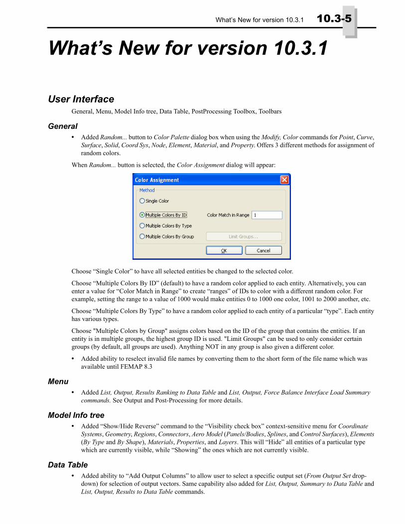
When Random... button is selected, the Color Assignment dialog will appear:
Choose “Single Color” to have all selected entities be changed to the selected color.
Choose “Multiple Colors By ID” (default) to have a random color applied to each entity. Alternatively, you can enter a value for “Color Match in Range” to create “ranges” of IDs to color with a different random color. For example, setting the range to a value of 1000 would make entities 0 to 1000 one color, 1001 to 2000 another, etc.
Choose “Multiple Colors By Type” to have a random color applied to each entity of a particular “type”. Each entity has various types.
Choose "Multiple Colors by Group" assigns colors based on the ID of the group that contains the entities. If an entity is in multiple groups, the highest group ID is used. "Limit Groups" can be used to only consider certain groups (by default, all groups are used). Anything NOT in any group is also given a different color.
• Added ability to reselect invalid file names by converting them to the short form of the file name which was available until FEMAP 8.3
Menu• Added List, Output, Results Ranking to Data Table and List, Output, Force Balance Interface Load Summary
commands. See Output and Post-Processing for more details.
Model Info tree• Added “Show/Hide Reverse” command to the “Visibility check box” context-sensitive menu for Coordinate
Systems, Geometry, Regions, Connectors, Aero Model (Panels/Bodies, Splines, and Control Surfaces), Elements (By Type and By Shape), Materials, Properties, and Layers. This will “Hide” all entities of a particular type which are currently visible, while “Showing” the ones which are not currently visible.
Data Table• Added ability to “Add Output Columns” to allow user to select a specific output set (From Output Set drop-
down) for selection of output vectors. Same capability also added for List, Output, Summary to Data Table and List, Output, Results to Data Table commands.

10.3-6 Finite Element Modeling
PostProcessing Toolbox• In the Freebody tool, added “Select Free Edge Nodes” icon button to Freebody Nodes section. This allows the
user to quickly and automatically choose the “free edge” nodes of the selected elements when Display Mode is set to “Interface Load”.
Toolbars• When using the “Create Group...” command from the “Selector Actions” menu of the Select Toolbar, the user is
now able to select any existing group when using the “Add to Group”, “Remove from Group”, or “Exclude from Group” options. Previously, these options only worked with the “active” group in the model.
• When Solid, Region, Connector, CSys, Material, or Property is the “active” entity in the Select Toolbar, the context-sensitive menu now includes a Visibility submenu, which contains 5 commands to change the visibility of selected entities.
In addition, if you hold down the Shift key while clicking the Right Mouse button, only the commands on the Visi-bility submenu will appear in the context-sensitive menu.
Meshing• Added Delete All button to dialog box of Mesh, Mesh Control, Custom Size Along Curve command.
• Added ability to specify a different Property when using the Mesh, Copy/Radial Copy/Scale/Rotate/Reflect, Element commands. Default is “0..Match Original”. Only elements which share a common topology with typi-cal elements of the selected property will be changed. All other elements will retain their original properties.
Loads and Constraints• Updated Model, Load, From Freebody command.
This command creates loads directly from a freebody display. Freebody display is controlled by the Freebody Tool in the PostProcessing Toolbox (see Section 7.2.3.3, "Freebody tool" for more information). You must have at least one Freebody entity defined in the model to use this command.
In the Create Load(s) from Freebody dialog box, select any number of existing Freebody entities from the Freebod-ies section, along with any number of existing Output Sets from the Output Set(s) section.
In the Loads section of the dialog box, choose a destination for the newly created force and/or moment loads. If a single Freebody using a single Output Set is selected, the newly created loads can be placed in an existing Load Set selected by the user or a new Load Set. Otherwise, the forces and/or moments from each Freebody/Output Set com-
Command DescriptionShow Selected Only
Sets visibility for all selected entities of the Entity Type currently active in the Select Tool-bar to “on”, while setting all others to “off”
Hide Selected Sets visibility for all selected entities of the “active” Entity Type to “off”Show All Sets visibility to “on” for all entities of the “active” Entity Type.Hide All Sets visibility to “off” for all entities of the “active” Entity Type.Show/Hide Reverse
Sets visibility to “off” for all entities of the “active” Entity Type which are currently visible, while setting visibility to “on” for all entities of the “active” Entity Type which are currently not visible.

Views 10.3-7
bination will always be placed into a new Load Set. For example, if 2 Freebodies and 4 Output Sets are selected, 8 new Load Sets will be created.
If “Force Vector Display” is set to “Off” in the Freebody Tool for a particular Freebody, then no Force loads will be created. Same is true about Moment loads if “Moment Vector Display” is set to “Off”. Use the Sum Data on Nodes option in the Freebody Tool to display exactly what will be created in the new or selected existing Load Set.
The user also has the ability to “Include Freebody Interface Load” and/or “Include Freebody Nodal Load(s)”. These options determine which loads will be created. If “Display Mode” is set to “Freebody” in the Freebody Tool, only the setting of “Include Freebody Nodal Load(s)” will be used when creating loads.
Finally, there is an option to “Create Single Load Definition for Freebody Nodal Loads”. When on, a single Load Definition will be created in each Load Set containing the various Freebody Nodal loads.
Views• Added “Right-Hand Rule First Edge” option to the Normal Style of the “Element - Directions” option in
“Labels, Entities and Color” Category of View, Options command. Much like the “Right-Hand Rule” option, except the arrow points from the first node to the second node.
• Added Reverse button to the Coord Sys, Connection, Aero Spline/Control Surface, Material, Property, and Layer tab to View, Visibility command. This will “Hide” all entities of a particular type which are currently visi-ble, while “Showing” the ones which are not currently visible.
Output and Post-Processing• Added ability to “Override Vector View Options” directly from the Contour Vector options dialog box. Previ-
ously, this option could only be toggled on/off using the “2D Tensor Plot View Options Override” option in the Views tab of the File, Preferences command.
• Added ability to use Entity IDs (Element, Material, or Property) when plotting a Contour, a Criteria Plot, or a Beam Diagram when using the View, Advanced Post, Contour Model Data command.
• Added ability to “Rank” selected results in the Data Table using the List, Output, Results Ranking to Data Table command.
This command provides a flexible tool to quickly display the top “n” ranked (max/min/or max absolute value) results for a set of selected output vector(s) in selected output set(s). The data can be ranked for each selected Node ID, selected Element ID, or selected elements of each Property ID or Material ID. Other options include “individ-
Note: Creating a single Load Definition may or may not be useful considering that almost all load values will be different. One positive aspect of creating a single Load Definition is deletion of all loads cre-ated by this command in a particular Load Set is very easy. One drawback is editing loads, as the val-ues of all loads in the Load Definition will be changed to a single value entered by the user.

10.3-8 Finite Element Modeling
ual” ranking based on the values in each output vector or an “overall” ranking using the values of all selected out-put vectors. FEMAP sends the “ranked data” to the Data Table dockable pane, where you can further group, sort, and filter the data to find the critical values you need.
When you choose this command you will see the following dialog box:
Method
Choose between two methods in this section, Sets for Each Entity or Entities for Each Set.
When using Sets for Each Entity, the listing will be displayed in the Data Table based on each selected entity (i.e., there will be a separate ranking for each Node, Element, Property, or Material ID).
When using Entities for Each Set, the listing will be sent to the Data Table based on each selected Output Set (i.e., there will be a separate ranking for each Output Set).
Rank By
Choose to rank by Node ID, Element ID, the elements of each Property, or the elements of each Material. Only Properties and Materials which are referenced by the selected elements will be included in the listing.
Approach
The Each Vector Individually option will rank based on the “highest ranking” values of each selected output vector, while All Vectors Together only ranks using the “highest ranking” values of all the selected output values together.
Ranking Type
Choose between ranking the output values using Max Value, Min Value, or Max Absolute Value. Also, enter a value for Number to Rank. In most cases (see Note below), this is the number of “ranked values” FEMAP will list to the Data Table for each Node, Element, Material, or Property ID.
Note: Depending on the selected output vectors, the All Vectors Together option may or may not be useful. For instance, if both “Top” and “Bottom” stresses of a certain type are being ranked, the user may sim-ply want the “highest stresses”. In this case, using the the All Vectors Together makes sense, since the stress being “Top” or “Bottom” is really not important. On the other hand, using All Vectors Together while ranking selected Stress and Strain vectors would be of no use, as it is highly likely only Stresses would be ranked when using Max Value, while only Strains would be ranked when using Min Value.
Note: If Method is set to Sets for Each Entity, Rank By is set to Node or Element, and the value of Number to Rank exceeds the number of selected Output Sets, FEMAP will only report rankings up to the number of selected Output Sets. Setting the Number to Rank to a smaller value than the number of selected Out-put Sets will only display the Number to Rank.
For example, if Number to Rank is set to “10”, but only “5” Output Sets are selected, the ranking will only be from 1-5, one value for each output set. Conversely, if Number to Rank was set to “3” and “5” Output Sets are selected, only the 3 “highest ranked” values for each selected node or element from the 5 possible values (one value for each Output Set) will be sent to the Data Table.

Output and Post-Processing 10.3-9
Select Output to Rank
The Select Output to Rank dialog box allows you to choose Output Sets and Output Vectors to be used for ranking in the Data Table.
Along with checking and unchecking the boxes, you can also highlight the selected Output Set or Output Vector and click the Toggle Selected Sets or Toggle Selected Vectors buttons, respectively.
If you check Select Similar Layer/Ply/Corner Vectors, you can select all similar data without worrying about checking all of the individual output vectors. For example, if you turn on this option, and select the vector "Plate Bot Von Mises Stress" (the centroidal Von Mises Stress at the bottom fiber of a plate/shell element), you will auto-matically also get the centroidal Von Mises Stress at the top fiber. If you also have Include Components/Corner Results selected, you will get the bottom and top Von Mises Stress at all of the element corners. Similarly, for lam-inate elements, this option allows you to select results for all plys without having to select them manually. When using this option it does not matter which output vector location you choose, you will get the similar data for all locations.
Once finished, click OK and view the Results Ranking in the Data Table
Data in the ReportDepending on the selected options, various columns will be sent to the Data Table. Also, the Show/Hide Group Header option in Data Table will always be “on”. When Method is set to “Sets for Each Entity”, the entity type selected in the Rank By section will be by itself as a “Group Header” (i.e., “Node ID”, “Element ID”, “Property ID” or “Material ID”. When Method is set to “Entities for Each Set”, the “Group Header” will always be “Set ID”.
Some commonly seen columns will be:
Rank - Value of “ranked” output values
Set ID - Output Set ID where ranked value is located
Node ID, Element ID, Material ID, and Property ID - IDs of entity type selected in Rank By section.
Vector ID - Output Vector ID where ranked value is located (Approach set to “All Vectors Together”)
Max, Min, or Max Abs - actual Max Value/Min Value/Max Absolute Value output values

10.3-10 Finite Element Modeling
Here are some examples:
Example 1 - Method set to “Sets for Each Entity”, Rank By set to “Node”, Approach set to “Each Vector Individu-ally”, Ranking Type set to “Max Value”, and Number to Rank set to “5”. Four Output Sets and “T1 Translation”, “T2 Translation”, and “T3 Translation” selected:
Notice, there were only 4 output sets selected, therefore the values could only be ranked 1-4. Also, the “Set ID” shows which output set the “highest ranking” value was found for each vector, for each node.
Example 2 - Method set to “Sets for Each Entity”, Rank By set to “Element”, Approach set to “All Vectors Together”, Ranking Type set to “Max Value”, and Number to Rank set to “5”. Four Output Sets and both “Plate Top X Normal Stress” and “Plate Bot X Normal Stress” selected:
Notice, only the title of the first output vector (chronologically, by output vector ID) is listed, then all other output vectors which are being ranked “together” are shown with a “+ (output vector ID)”. The “Vector ID” column shows which output vector produced the “highest ranking” value in each output set. Again, only 4 output sets were selected, so the rankings only go from 1-4, even though Number to Rank was set to “5”.
Example 3 - Method set to “Sets for Each Entity”, Rank By set to “Property”, Approach set to “Each Vector Indi-vidually”, Ranking Type set to “Min Value”, and Number to Rank set to “5”. Four Output Sets and “Plate Top Von-Mises Stress” selected:

Output and Post-Processing 10.3-11
Notice, this time the rankings go from 1-5. In this case, the minimum values all come from the same output set, and the individual element IDs where the ranked values can be found are also listed.
Example 4 - Method set to “Entities for Each Set”, Rank By set to “Material”, Approach set to “Each Vector Indi-vidually”, Ranking Type set to “Max Value”, and Number to Rank set to “5”. Four Output Sets and “Plate X Mem-brane Force” selected:
Notice, the results are now ranked within each Output Set. In this case, all the elements with the highest ranking values using “Max Value” all happen to be made of the same Material.
If Ranking Type had been set to “Max Absolute Value” instead, the top 5 Force values are all negative, but have a greater magnitude than the values ranking in the Data Table when using “Max Value”.
This is one case where having the Ranking Type set to “Max Absolute Value” is probably better to determine the “worst case” when examining this output vector for these particular analyses.

10.3-12 Finite Element Modeling
• Added List, Output, Force Balance Interface Load Summary command.
This command lists Force and Moment values for the “Interface Load” portion of a single selected Freebody entity across any number of selected Output Sets OR any number of selected Freebody entities in a single selected Output Set. This command will only list values from Freebody entities with the Display Mode set to “Interface Load”. In addition to listing this information to the Messages window, the command can also create FEMAP Functions which can then be examined via XY plot. .
Summary Mode
This command has 2 different modes:
Single Freebody, Multiple Output Sets - select a single Freebody entity from the Freebodies list, then any number of output sets from the Output Sets list. The listing below is for a single Freebody and 4 selected output sets::
The listing will always include Fx, Fy, Fz, Mx, My, and Mz values for each Output Set. If the Consider Interface Load Resultant option is “on” (default), then a “Force Resultant” (FR) and “Moment Resultant” (MR) will also be
Note: To select multiple Freebody entities or Output Sets, hold down Ctrl while clicking to select them individ-ually or Shift to choose a “range”.
Output and Post-Processing 10.3-13
listed. A Max Value and a Min Value for each Component and Resultant across all selected Output Sets is also cal-culated and listed, along with the output set where the max/min values occur. Additional information such as “Components included in the summation”, “Contributions included in summation”, and “Summation about” loca-tion are also listed for reference purposes.
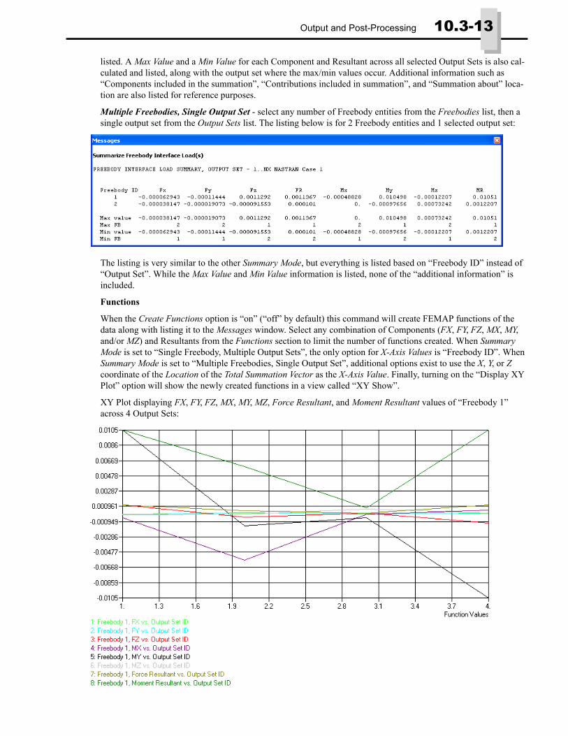
Multiple Freebodies, Single Output Set - select any number of Freebody entities from the Freebodies list, then a single output set from the Output Sets list. The listing below is for 2 Freebody entities and 1 selected output set:
The listing is very similar to the other Summary Mode, but everything is listed based on “Freebody ID” instead of “Output Set”. While the Max Value and Min Value information is listed, none of the “additional information” is included.
Functions
When the Create Functions option is “on” (“off” by default) this command will create FEMAP functions of the data along with listing it to the Messages window. Select any combination of Components (FX, FY, FZ, MX, MY, and/or MZ) and Resultants from the Functions section to limit the number of functions created. When Summary Mode is set to “Single Freebody, Multiple Output Sets”, the only option for X-Axis Values is “Freebody ID”. When Summary Mode is set to “Multiple Freebodies, Single Output Set”, additional options exist to use the X, Y, or Z coordinate of the Location of the Total Summation Vector as the X-Axis Value. Finally, turning on the “Display XY Plot” option will show the newly created functions in a view called “XY Show”.
XY Plot displaying FX, FY, FZ, MX, MY, MZ, Force Resultant, and Moment Resultant values of “Freebody 1” across 4 Output Sets:

10.3-14 Finite Element Modeling
Geometry InterfacesThe following FEMAP interfaces have been updated to support newer geometry formats:
• Added support to optionally read or skip “Free Points” during import of an IGES file.
For details, see “Geometry Interfaces” in the FEMAP User Guide.
Analysis Program InterfacesSeveral of the analysis program interfaces have been improved. These changes include:
• Nastran Interfaces (NX and MSC/MD)
• ANSYS Interface
Nastran Interfaces (NX and MSC/MD)• Added support for importing files with truncated INCLUDE statements
A number of bugs were corrected.
For details, see “Analysis Program Interfaces” in the FEMAP User Guide.
ANSYS InterfaceA number of bugs were corrected.
For details, see “Analysis Program Interfaces” in the FEMAP User Guide.
Tools• Added “Move Only, No Merge” option to Action drop-down in Tools, Check, Coincident Nodes command.
OLE/COM APINew API Methods• Added HasList and CountList for Group object
The following functions have been added:• feModifyColorMultiple
• feFileRecoverDBData
PreferencesDatabase• Added Recover _DBData File... button to off a different method to use when attempting to recover a corrupted
model file.
You should always try the Recover Scratch Directory command before attempting to use this command. The _DBData file exists in the Scratch Directory, but will usually never contain the complete contents of the model. Also, some of the data in this file may be in an unusable state. That said, this may be useful as a final attempt to recover portions of a corrupted model. A proper use of the option involves opening a new session of FEMAP, using the command, selecting the _DBData file, then manually removing any portion of the model which appears cor-rupt. Once manual clean up of the “recovered” model is completed, immediately export a FEMAP neutral file.
FEMAP Interface Latest Supported VersionParasolid Parasolid 24.1ACIS ACIS R22, SP1
Note: NEVER use this command when a properly working model is already open in FEMAP. Also, this com-mand is in no way a guaranteed method for recovering any portion of a corrupted model. It is simply provided to give the user an additional option when attempting to recover some model data.

What’s New for version 10.3 10.3-15
What’s New for version 10.3
User InterfaceGeneral, Entity Select, Menu, Toolbars, Model Info tree, Data Table, Entity Editor, Data Surface Editor, Meshing Toolbox, PostProcessing Toolbox
General• Added Filter Title and Clear Title Filter icon buttons to the Load Set, Constraint Set, Group, Layer, View, Solid,
and Freebody Manager dialog boxes.
• Only tabs of entity types which currently exist in the model will be displayed in the View, Visibility dialog box.
• User created Toolbars will now transfer between versions of FEMAP.
• Pressing Ctrl+M while in a dialog box field asking for a length will display the Select Curve to Measure dialog box, which will return the selected curves length.
• Added the Locate Center to the Methods for specifying the a coordinate.
The Locate Center method requires three specified locations which are not colinear to determine a “circle”. The “center” location is then determined by finding the center point of the “circle”. A geometric circular curve is NOT created.
Entity Select• Added “on Property” and “on CSys” methods when selecting Coordinate Systems.
Menu• Added Tools, Toolbars, Aeroelasticity command. See Toolbars section.
• Added Model, Aeroelasticity... commands (Panel/Body, Property, Spline, and Control Surface) to create the var-ious entities used in Static Aeroelastic analysis and Aerodynamic Flutter analysis. See Aeroelasticity section.
• Added Mesh, Geometry Preparation command. See Meshing section.
• Added commands to Modify, Edit..., Modify, Color..., Modify, Layer..., and Modify Renumber... menus for the Aeroelasticity entities (Aero Panel/Body, Aero Property, Aero Spline, and Aero Control Surface).
Center of ‘circle’
Location 1
Location 2
Location 3

10.3-16 Finite Element Modeling
• Added Modify, Update Other, Aero Interference Group command. Allows modification of IGID on any number of selected Aero Panel/Body entities at the same time.
• Added List, Output, Force Balance to Data Table and List, Output, Force Balance Interface Load to Data Table commands. Also, updated List, Output, Force Balance and List, Output, Force Balance Interface Load to use Freebody entities. See Freebody tool section.
• Added commands to Delete, Model... menu to delete the Aeroelasticity entities (Aero Panel/Body, Aero Prop-erty, Aero Spline, and Aero Control Surface
• Added Delete, Output, Freebody command to delete any number of selected Freebody entities.
• Added Group, Coord Sys, on Property and Group, Coord Sys, on CSys commands to add additional methods to add Coordinate Systems to groups.
• Added View, Align By, Surface and View, Align By, Normal to Plane commands to align the active view to either the normal of a selected planar surface or the normal of a specified plane, respectively.
Toolbars• Added Aeroelasticity Toolbar. Contains overall visibility controls (Draw Entity check box) of the Aero Panel,
Aero Mesh, Aero Spline, and Aero Control Surfaces options in the Labels, Entities and Color section of the View, Options command.
• Added Mesh Geometry Preparation icon to Mesh Toolbar. See Meshing section.
Model Info tree• Added Aero Model branch and underlying branches for Panels/Bodies, Properties, Splines, and Control Sur-
faces, which allow for creation, copying, editing, listing, and deleting of the various aeroelasticity entities. The color and layer may also be changed.
• Added Visibility check boxes (on/off) for Aero Model - Planels/Bodies, Splines, and Control Surfaces.
• Added Compare command to context-sensitive menu for Results. Provides that same functionality as the Model, Output, Compare command for the selected sets.
Data Table• Added a “Skew” column when using the “Add Element Checks” command.
Entity Editor• Added “Skew” field to Element Quality section when an element is loaded in the Editor.
Data Surface Editor• Added “Mapping Tolerance” to the “Options” of the Output Map Data Surface.
When a “Target” location is projected onto the “Source” data surface and the distance to a discrete data point is less than the tolerance, the “Source” value of the "coincident" location is directly mapped to the “Target” without inter-polation. If multiple nodes fall within this tolerance, then the first one encountered numerically will be directly mapped. Default value is the "Merge Tolerance" of the "Target” model.
Meshing Toolbox• Added Add Surface Mesh Point check box to Feature Removal tool (Feature Type = “Loops” only). Will create
a point at the “center” of the “loop”, then use that point as a “mesh point” on the surface. See Section 5.1.2.9, "Mesh, Mesh Control, Mesh Points on Surface..." for more information.
• Performance improvements to Propagate by Mapped Approach option in Mesh Sizing tool. Also, if no “mesh sizing exists on a curve, now the number of nodes attached is used for the initial mesh sizing.
PostProcessing Toolbox• Added Freebody tool to all facets of Freebody display post-processing.
PostProcessing Toolbox 10.3-17
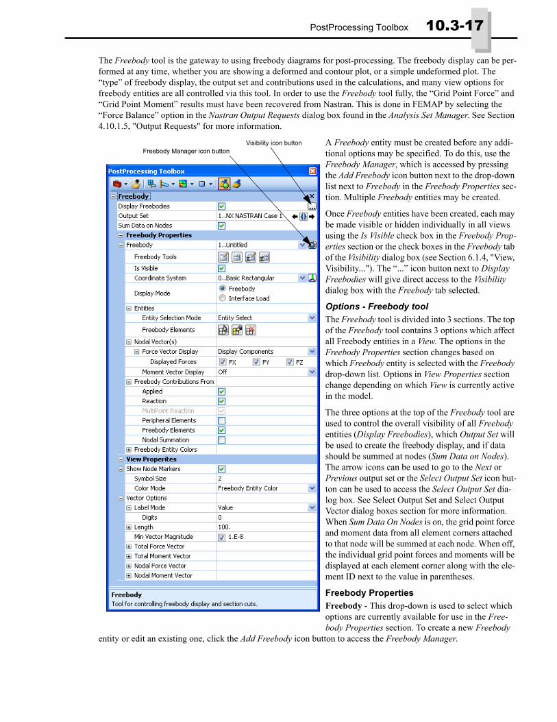
The Freebody tool is the gateway to using freebody diagrams for post-processing. The freebody display can be per-formed at any time, whether you are showing a deformed and contour plot, or a simple undeformed plot. The “type” of freebody display, the output set and contributions used in the calculations, and many view options for freebody entities are all controlled via this tool. In order to use the Freebody tool fully, the “Grid Point Force” and “Grid Point Moment” results must have been recovered from Nastran. This is done in FEMAP by selecting the “Force Balance” option in the Nastran Output Requests dialog box found in the Analysis Set Manager. See Section 4.10.1.5, "Output Requests" for more information.
A Freebody entity must be created before any addi-tional options may be specified. To do this, use the Freebody Manager, which is accessed by pressing the Add Freebody icon button next to the drop-down list next to Freebody in the Freebody Properties sec-tion. Multiple Freebody entities may be created.
Once Freebody entities have been created, each may be made visible or hidden individually in all views using the Is Visible check box in the Freebody Prop-erties section or the check boxes in the Freebody tab of the Visibility dialog box (see Section 6.1.4, "View, Visibility..."). The “...” icon button next to Display Freebodies will give direct access to the Visibility dialog box with the Freebody tab selected.
Options - Freebody toolThe Freebody tool is divided into 3 sections. The top of the Freebody tool contains 3 options which affect all Freebody entities in a View. The options in the Freebody Properties section changes based on which Freebody entity is selected with the Freebody drop-down list. Options in View Properties section change depending on which View is currently active in the model.
The three options at the top of the Freebody tool are used to control the overall visibility of all Freebody entities (Display Freebodies), which Output Set will be used to create the freebody display, and if data should be summed at nodes (Sum Data on Nodes). The arrow icons can be used to go to the Next or Previous output set or the Select Output Set icon but-ton can be used to access the Select Output Set dia-log box. See Select Output Set and Select Output Vector dialog boxes section for more information. When Sum Data On Nodes is on, the grid point force and moment data from all element corners attached to that node will be summed at each node. When off, the individual grid point forces and moments will be displayed at each element corner along with the ele-ment ID next to the value in parentheses.
Freebody PropertiesFreebody - This drop-down is used to select which options are currently available for use in the Free-body Properties section. To create a new Freebody
entity or edit an existing one, click the Add Freebody icon button to access the Freebody Manager.
Visibility icon buttonFreebody Manager icon button

10.3-18 Finite Element Modeling
• Freebody Manager - Used to create, edit, renumber, copy, and delete Freebody entities.
New Freebody - When clicked, the New Freebody dialog box will appear.
In this dialog box, specify an ID and Title (optional) along with some “top-level” options for the new Freebody entity, such as Display Mode , Vector Display Freebody Contributions, and Load Components in Total Summation. These options will be described later in this section
Update Title - Highlight a Freebody entity in Available Freebodies list, then click this button to enter a new Title.
Renumber - Highlight a Freebody entity in Available Freebodies list, then click this button to change the ID.
Delete - Highlight a Freebody entity in Available Freebodies list, then click this button to delete it from the model.
Delete All - Deletes all Freebody entities in the model.
Copy - Highlight a Freebody entity in Available Freebodies list, then click this button to make a copy.
None Active - When clicked, there is no longer an “Active” Freebody entity.
Title Filter Clear Title Filter

PostProcessing Toolbox 10.3-19
Default Settings - When clicked, the following options are set:
Display Mode: “Freebody Only”
Vector Display: “Nodal Forces” displayed as Components, “Nodal Moments” Off
Freebody Contributions: “Applied”, “Reaction”, “MultiPoint Reaction”, and “Peripheral Elements” On, “Freebody Elements” and “Nodal Summation” Off.
More - Click this button to create another new Freebody entity.
Freebody Tools - This section contains four icon buttons used for sending the data used in the calculations to cre-ate the freebody display to the Messages window or the Data Table.
• List Freebody to Messages Window - Lists all contributions used to create the display of the Freebody entity currently selected in the Freebody tool to the Messages window. ID is the node ID where the Nodal Force and Nodal Moment vectors are being calculated and Source is the Element ID which is providing the force and moment contributions.
Freebody to Messages
Freebody to Data Table Summation to Messages
Summation to Data Table
10.3-20 Finite Element Modeling
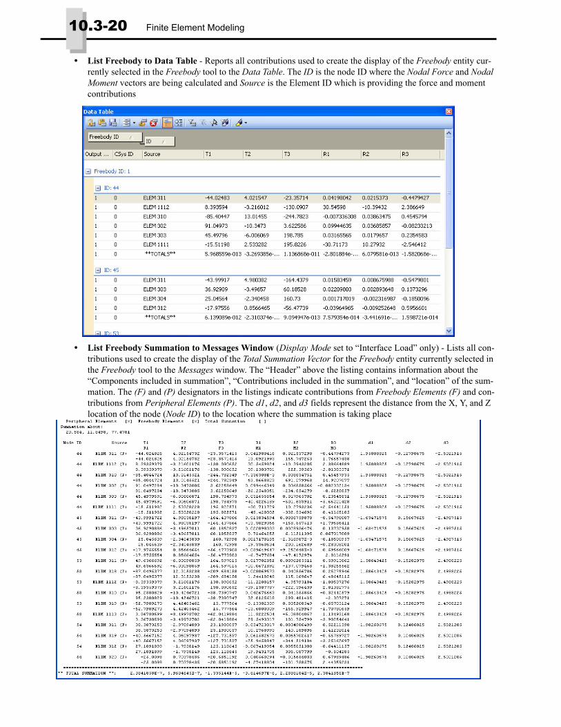
• List Freebody to Data Table - Reports all contributions used to create the display of the Freebody entity cur-rently selected in the Freebody tool to the Data Table. The ID is the node ID where the Nodal Force and Nodal Moment vectors are being calculated and Source is the Element ID which is providing the force and moment contributions
• List Freebody Summation to Messages Window (Display Mode set to “Interface Load” only) - Lists all con-tributions used to create the display of the Total Summation Vector for the Freebody entity currently selected in the Freebody tool to the Messages window. The “Header” above the listing contains information about the “Components included in summation”, “Contributions included in the summation”, and “location” of the sum-mation. The (F) and (P) designators in the listings indicate contributions from Freebody Elements (F) and con-tributions from Peripheral Elements (P). The d1, d2, and d3 fields represent the distance from the X, Y, and Z location of the node (Node ID) to the location where the summation is taking place

PostProcessing Toolbox 10.3-21
• List Freebody Summation to Data Table (Display Mode set to “Interface Load” only) - Reports all the same information as List Freebody Summation to Messages Window, but sends it to the Data Table. One difference is that the “Header” information is still sent to the Messages window, as there is no logical place to report this information in the Data Table.
Is Visible - When On, the Freebody entity currently in the Freebody drop-down will be visible in the graphics win-dow in all views. Display of Freebody entities may also be controlled via the Freebody tab of the Visibility dialog box.
Coordinate System - Drop-down list specifies which coordinate system should be used to display the freebody vectors. You can create a new coordinate system by using the New Coord Sys icon button.
Display Mode - Each Freebody entity can be displayed in two different modes, Freebody or Interface Load.
• Freebody - Only Freebody Elements may be selected in the Entities section and only the vectors in the Nodal Vector(s) section can be displayed and controlled.
• Interface Load - Both Freebody Nodes and Freebody Elements must be selected in the Entities section and vectors in both the Nodal Vector(s) and the Total Summation Vector sections can be displayed and controlled. Additionally, a Location must be selected when using this option.
Entities - Allows you to specify which Freebody Elements (Display Mode = “Freebody”) or Freebody Nodes and Freebody Elements (Display Mode = “Interface Load”) are used by a Freebody entity. Based on the Entity Selection Mode, elements and nodes may be selected for the Freebody entity directly or by using a pre-defined group.
• Entity Selection Mode - When set to Entity Select, elements and nodes are selected, highlighted in the graphics widow, or deleted from the Freebody entity using the icon buttons below. An additional icon button exists for placing the summation location at the center of the selected nodes.
When set to Group Select, elements and nodes are determined by selecting a group from the Group drop-down list. If Group is set to “-1..Active”, then the elements will be retrieved from the Active group in the model. The Group Manager dialog box may also be accessed by the icon button next to the Group drop-down (see Section 6.4.3.1, "Group, Create/Manage..." for more information).
Total Summation Vector (Display Mode set to “Interface Load” only) - Allows you to specify the Location of the Total Force Vector and Total Moment Vector, along with how these vectors are displayed and what components will be summed to create these vectors.
• Location - Allows you to specify the location of summation for the Total Summation Vector. Click the icon but-ton next to location to pick a location from the graphics window. Additionally, the individual coordinates may be entered or edited below the Location, when expanded.
Note: Only entities which can be displayed and controlled by the selected Display Type will be available in the Freebody Entity Colors section, while setting the View Properties for all the different freebody vector types and nodes markers is available at all times.
Select Elements
Highlight Elements in Freebody
Delete Elements
Highlight Selected Nodes
Display Mode = Freebody Display Mode = Interface Load
from Freebodyfor Freebody Select Nodesfor Interface Load
for Interface Load Delete Elementsfrom Freebody
Place Summationpoint at center ofSelected Nodes

10.3-22 Finite Element Modeling
When nodes are selected in the Entities section, the user will be prompted to answer the following question:
Auto-locate total summation vector at center of freebody nodes (“X-coordi-nate”, “Y-coordinate”, “Z-coordinate” in coordinate system “ID of Coordi-nate System specified in Freebody Properties”)?
If you click Yes, the Location will be specified at the center of the selected nodes. If you click No, the Location will be at (0.0, 0.0, 0.0) or the Location last used by the Freebody entity cur-rently in the Freebody tool.
• Force Vector Display - This option controls how the “Force vector” (single arrow head) of the Total Summa-tion Vector will be displayed. When set to “Off”, the force vector will be not be displayed. When set to “Display Components”, the force vector will be displayed in X, Y, and/or Z Components (individual components may be toggled on/off using the FX, FY, and FZ check boxes for Displayed Forces). When set to “Display Resultant”, the force vector will be displayed as a single resultant vector based on the components currently “on” in Dis-played Forces.
• Moment Vector Display - This option controls how the “Moment vector” (double arrow head) of the Total Summation Vector will be displayed. When set to “Off”, the moment vector will be not be displayed. When set to “Display Components”, the moment vector will be displayed in X, Y, and/or Z Components (individual com-ponents may be toggled on/off using the MX, MY, and MZ check boxes for Displayed Moments). When set to “Display Resultant”, the moment vector will be displayed as a single resultant vector based on the components currently “on” in Displayed Moments.
• Summed Components - This option controls which Force and Moment components will be used to calculate the Total Summation Vector. Turning individual Force components on/off is also very likely to affect the Moment values, so keep that in mind.
Following figures show the Total Summation Vector. Freebody Node Markers are “On”, Node Vector(s) not dis-played, Element Transparency set to 75%, and Element Shrink View Option is “On”.
Nodal Vector(s) - Allows you to control how the Force and Moment vectors are displayed at each node (Sum Data on Nodes in View Properties section “On”) or each “element corner” (Sum Data on Nodes “Off”).
• Force Vector Display - This option controls how the “Force vectors” (single arrow head) are displayed. When set to “Off”, the force vectors will be not be displayed. When set to “Display Components”, the force vector at each node/element corner will be displayed in X, Y, and/or Z Components (individual components may be tog-
Display Mode = Interface LoadTotal Summation Vector Force and Moment set to “Display Resultant”
Display Mode = Interface LoadTotal Summation Vector Force set to “Off”and Moment set to “Display Components”

PostProcessing Toolbox 10.3-23
gled on/off using the FX, FY, and FZ check boxes for Displayed Forces). When set to “Display Resultant”, the force vector at each node/element corner will be displayed as a single resultant vector based on the components currently “on” in Displayed Forces.
• Moment Vector Display - This option controls how the “Moment vectors” (double arrow head) are displayed. When set to “Off”, the moment vectors will be not be displayed. When set to “Display Components”, the moment vector at each node/element corner will be displayed in X, Y, and/or Z Components (individual compo-nents may be toggled on/off using the MX, MY, and MZ check boxes for Displayed Moments). When set to “Dis-play Resultant”, the moment vector at each node/element corner will be displayed as a single resultant vector based on the components currently “on” in Displayed Moments..
When Sum Data on Nodes is “On”, the Nodal Vector(s) will be at each node:
When Sum Data on Nodes is “Off”, the Nodal Vector(s) at each element corner will include the Element ID
Freebody Contributions From - Allows you to control the calculation of the Freebody entity by choosing which contributions should be included. Available contributions are from Applied Loads, from Reaction Forces and Moments at single point constraints and/or constraint equations, from the selected elements (Freebody Elements), and from the elements surrounding the Freebody Elements (Peripheral Elements). Toggling various options on/off can drastically alter the values and appearance of a Freebody entity, so be sure to have the proper contributions included for your particular needs.
• Applied - When On, includes contributions from all loads applied to the model used to produce the results in the selected Output Set.
• Reaction - When On, includes contributions from all reaction forces and moments at single point constraints in the model used to produce the results in the selected Output Set.
• MultiPoint Reaction - When On, includes contributions from all reaction forces and moments from constraint equations, rigid elements, and interpolation elements in the model used to produce the results in the selected Output Set.
Display Mode = FreebodyNodal Vector(s): Force Set to “Display Components”, Moment set to “Off”
Display Mode = FreebodyNodal Vector(s): Force Set to “Off”, Moment set to “Display Resultant”
Forces shown using “Display Components” at “element corners” Moments shown using “Display Components” at “element corners”

10.3-24 Finite Element Modeling
• Peripheral Elements - When On, includes grid point force and moment contributions from the selected Output Set for the elements surrounding the Freebody Elements selected in Entities section.
• Freebody Elements - When On, includes grid point force and moment contributions from the selected Output Set for the elements selected in Entities section.
• Nodal Summation - When On, includes force and moment contributions from nodal summation. Typically, these are very small numbers, unless there is a “non-balanced” force or moment in the model.
Freebody Entity Colors - Allows you to specify colors for Node Marker(s), Total Force Vector, Total Moment Vector, Nodal Force Vector(s), and/or Nodal Moment Vector(s) for each Freebody entity. Click the icon button to select a color from the Color Palette. These colors will only be used when the “Color Mode” for any of these items is set to “Freebody Entity Color” in the View Properties section of the Freebody tool or via the Freebody... options in the View Options dialog box, PostProcessing category (See Section 8.3.25, "Freebody options").
View PropertiesThe View Properties control the visibility, style, color, and labeling for Freebody display. Each view in the model can have different options set in the section. When a different view is activated, the values from that view will fill the View Properties section.
Show Node Markers - controls the visibility, symbol size, and color of the “node markers” for Freebody entities. Having the node markers visible is a good way to visually inspect the nodes or element corners being used in the freebody calculations. The Symbol Size can be entered directly or increased/decreased using the “slider bar”. When Color Mode is set to “Freebody Entity Color”, the node markers will use the color specified for Freebody Node Marker(s) in the Freebody Properties section.
Vector Options - controls the Label Mode, Length, and Label Format of the Freebody vectors. Label Mode allows you to display No Labels, the Value of each freebody vector, or the value using exponents. For Label Format, the number of digits may be entered directly or increased/decreased using the “slider bar”. This will chance the number of significant digits being displayed. When Label Format is set to “0”, this is an “automatic mode” and FEMAP will determine the number of significant digits to display.
When Adjust Length is “off”, the length of each freebody vector “type” is controlled by a combination of the entered Length value and the Factor value entered for the Freebody Total Force, Freebody Total Moment, Freebody Nodal Force, and Freebody Nodal Moment view options.
When Adjust Length is “on”, the length of the freebody vectors will be adjusted based on the vector’s value (i.e., larger values = longer vectors). The Units/Length value is an additional parameter used to control the length of the vectors when in this mode. Essentially, the Units/Length value is used in the following manner:
If Units/Length value is 250, then a freebody vector value of 500 would be shown using a length of “2*Factor” on the screen. For the same freebody vector value of 500, entering a Units/Length value of 100 would display the vec-tor using a length of “5*Factor” on the screen.
Min Vector Magnitude - allows you to set a tolerance below which the vectors are not displayed. Using the default value of 1.0E-8, this option will basically remove vectors from the display that are not zero just due to numerical round-off. The value can also be used as a cut-off value, so if it is set to 10, only vector values above 10 will be dis-played.
Contributions = Applied, Reaction, and Peripheral Elements Contributions = Applied, Reaction, and Freebody ElementsFreebody Elements = 75% Transparent in figure Peripheral Elements = 75% Transparent in figure
Sum Data on Nodes = Off, Freebody Node Markers = OnSum Data on Nodes = On, Freebody Node Markers = On

Geometry 10.3-25
Total Force Vector/Total Moment Vector - controls the Vector Style, Color Mode, and Factor for the Total Sum-mation Force and Moment vectors. The Total Summation vectors are only visible when the Display Mode of a Freebody entity is set to “Interface Load”.
When Vector Style is set to Arrow or Center Arrow, the vectors will be displayed as lines. When set to Solid Arrow or Center Solid Arrow, the vectors will be “thicker, filled-in solids”. Factor is an additional scale factor which can be entered to change the size of the selected vector type.
When Color Mode is set to Freebody Entity Color, the “Freebody Entity Colors” specified for each Freebody entity in the Freebody tool is used. This allows multiple Freebody entities to be displayed at one time using unique colors for clarity. RGB Color uses Red to display the X component, Green for the Y component, and Blue for the Z com-ponent of each vector.
Nodal Force Vector/Nodal Moment Vector - offers the same options as Freebody Total Force/Freebody Total Moment, but these options control the Nodal Vector(s). One difference is in Color Mode, where an additional option, Source Color exists. When set to Source Color, this selected vector type uses the color of the “source” ele-ments, the color of the load for Applied loads, and/or the color of the constraint for Reaction forces and moments. When the Sum Data on Nodes option is “on” and Source Color is selected, the View Color will be used.
Geometry• Enhanced Geometry, Solid, Embed to allow embedding of multiple solids into the base solid all at once.
Meshing• Enhanced “Suppress Short Edges” option in Mesh, Mesh Sizing, Size on Surface and Mesh, Mesh Sizing, Size
on Solid to be a percentage of Mesh Size instead of a percentage of “average curve length” on selected geome-try.
• Added Mesh, Geometry Preparation command
This command uses a set of parameters to find situations in geometry which typically result in poor element qual-ity, then uses a combination of automatic curve/surface splitting, creation of Combined Curves/Boundary Surfaces, and feature suppression to likely improve mesh quality. In addition, this command will “prepare” some parts to a degree which will allow FEMAP to successfully mesh the part.
In most cases, this automatic process will be all that is need to produce a good quality mesh. However, even if it cannot fully automatically produce an acceptable mesh, it will still provide a good starting point for using the other interactive geometry cleanup tools, and greatly reduce the amount of work required.
Surfaces and Curves which have loads or boundary conditions applied will be ignored.
By default, the command goes through two steps, Prepare Geometry and Mesh Sizing. You can choose to skip either step by simply un-checking the box next to Prepare Geometry or Mesh Sizing. The value for size shown for
Note: If FEMAP is successful when meshing a solid with acceptable mesh quality for your application, then using “Mesh, Geometry Preparation” is probably not necessary. Also, please be aware when using this process, it is quite common for certain small features to be ignored or removed completely.
Note: It is recommended to use the “Mesh, Geometry Preparation” command BEFORE manually creating additional Combined Curves /Boundary Surfaces for meshing purposes.
10.3-26 Finite Element Modeling
both Prepare Geometry and Mesh Sizing is the “Default Mesh Size” calculated by FEMAP (uses the same algo-rithm as "Mesh, Geometry, Solids").
Prepare GeometryThe value for Prepare Geometry is simply used as a baseline value for the various Prepare Options. Therefore, it is typically a good idea to change the Prepare Geometry value instead of the individual Prepare Options values.
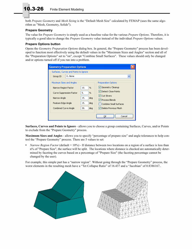
Prepare Options buttonOpens the Geometry Preparation Options dialog box. In general, the "Prepare Geometry" process has been devel-oped to function most effectively using the default values in the "Maximum Sizes and Angles" section and all of the "Preparation Options" set to "on", except "Combine Small Surfaces". These values should only be changed and/or options turned off if you run into a problem.
Surfaces, Curves and Points to Ignore - allows you to choose a group containing Surfaces, Curves, and/or Points to exclude from the "Prepare Geometry" process.
Maximum Sizes and Angles - allows you to specify “percentage of prepare size” and angle tolerances to help con-trol the “Prepare Geometry” process. There are 5 values to set:
• Narrow Region Factor (default = 10%) - If distance between two locations on a region of a surface is less than n% of "Prepare Size", the surface will be split. The locations where distance is checked are automatically deter-mined by faceting the curves based on a percentage of "Prepare Size" (the faceting percentage cannot be changed by the user).
For example, this simple part has a “narrow region”. Without going through the “Prepare Geometry” process, the worst elements in the resulting mesh have a “Tet Collapse Ratio” of 16.437 and a “Jacobian” of 0.8386167..

Meshing 10.3-27
Zoomed-in view of “narrow region” at the corner of the part:
After the “Prepare Geometry” process using the defaults, the “narrow region” has been split from the original sur-face, then combined with surfaces from the “base”. Also, two short curves at the split locations have been sup-pressed. Finally, 2 Combined Curves have been created to allow larger elements in an area that used to be restricted by the “narrow region” Worst elements now have “Tet Collapse Ratio” of 5.67 and “Jacobian” of 0.694
.
Close-up of “narrow region” split
Close-up of Combined Curve and
“Split Curve” is suppressed
Boundary Surfaces at Corner
10.3-28 Finite Element Modeling
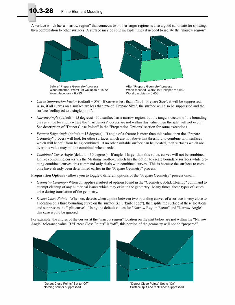
A surface which has a “narrow region” that connects two other larger regions is also a good candidate for splitting, then combination to other surfaces. A surface may be split multiple times if needed to isolate the “narrow region”.
• Curve Suppression Factor (default = 5%)- If curve is less than n% of "Prepare Size", it will be suppressed. Also, if all curves on a surface are less than n% of "Prepare Size", the surface will also be suppressed and the surface "collapsed to a single point".
• Narrow Angle (default = 15 degrees) - If a surface has a narrow region, but the tangent vectors of the bounding curves at the locations where the "narrowness" occurs are not within this value, then the split will not occur. See description of "Detect Close Points" in the "Preparation Options" section for some exceptions.
• Feature Edge Angle (default = 15 degrees) - If angle of a feature is more than this value, then the "Prepare Geometry" process will look for other surfaces which are not above this threshold to combine with surfaces which will benefit from being combined. If no other suitable surface can be located, then surfaces which are over this value may still be combined when needed.
• Combined Curve Angle (default = 30 degrees) - If angle if larger than this value, curves will not be combined. Unlike combining curves via the Meshing Toolbox, which has the option to create boundary surfaces while cre-ating combined curves, this command only deals with combined curves. This is because the surfaces to com-bine have already been determined earlier in the "Prepare Geometry" process.
Preparation Options - allows you to toggle 6 different options of the “Prepare Geometry” process on/off.
• Geometry Cleanup - When on, applies a subset of options found in the "Geometry, Solid, Cleanup" command to attempt cleanup of any numerical issues which may exist in the geometry. Many times, these types of issues arise during translation of the geometry.
• Detect Close Points - When on, detects when a point between two bounding curves of a surface is very close to a location on a third bounding curve on the surface (i.e., "knife edge"), then splits the surface at these locations and suppresses the "split curve". Using the default values for "Narrow Region Factor" and "Narrow Angle", this case would be ignored.
For example, the angles of the curves at the “narrow region” location on the part below are not within the “Narrow Angle” tolerance value. If “Detect Close Points” is “off”, this portion of the geometry will not be “prepared”..
Before “Prepare Geometry” processWhen meshed, Worst Tet Collapse = 15.72Worst Jacobian = 0.793
After “Prepare Geometry” processWhen meshed, Worst Tet Collapse = 4.642Worst Jacobian = 0.458
“Detect Close Points” Set to “Off” “Detect Close Points” Set to “On”Nothing split or suppressed Surface split and “split line” suppressed
Meshing 10.3-29
• Cut Slivers - When on, will review all surfaces considered "slivers" and determine if they should be "cut" again to allow for more effective combining with adjacent surfaces.
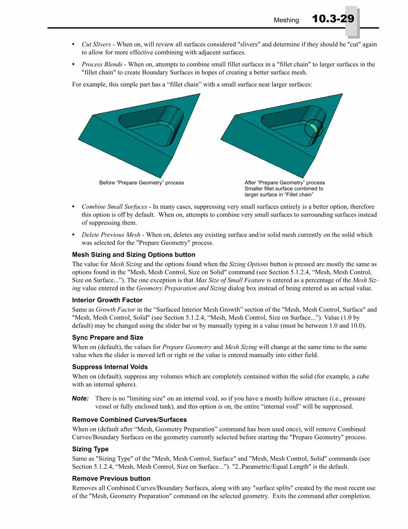
• Process Blends - When on, attempts to combine small fillet surfaces in a "fillet chain" to larger surfaces in the "fillet chain" to create Boundary Surfaces in hopes of creating a better surface mesh.
For example, this simple part has a “fillet chain” with a small surface near larger surfaces:
• Combine Small Surfaces - In many cases, suppressing very small surfaces entirely is a better option, therefore this option is off by default. When on, attempts to combine very small surfaces to surrounding surfaces instead of suppressing them.
• Delete Previous Mesh - When on, deletes any existing surface and/or solid mesh currently on the solid which was selected for the "Prepare Geometry" process.
Mesh Sizing and Sizing Options button The value for Mesh Sizing and the options found when the Sizing Options button is pressed are mostly the same as options found in the "Mesh, Mesh Control, Size on Solid" command (see Section 5.1.2.4, “Mesh, Mesh Control, Size on Surface...”). The one exception is that Max Size of Small Feature is entered as a percentage of the Mesh Siz-ing value entered in the Geometry Preparation and Sizing dialog box instead of being entered as an actual value.
Interior Growth FactorSame as Growth Factor in the “Surfaced Interior Mesh Growth” section of the "Mesh, Mesh Control, Surface" and "Mesh, Mesh Control, Solid" (see Section 5.1.2.4, “Mesh, Mesh Control, Size on Surface...”). Value (1.0 by default) may be changed using the slider bar or by manually typing in a value (must be between 1.0 and 10.0).
Sync Prepare and SizeWhen on (default), the values for Prepare Geometry and Mesh Sizing will change at the same time to the same value when the slider is moved left or right or the value is entered manually into either field.
Suppress Internal VoidsWhen on (default), suppress any volumes which are completely contained within the solid (for example, a cube with an internal sphere).
Remove Combined Curves/SurfacesWhen on (default after “Mesh, Geometry Preparation” command has been used once), will remove Combined Curves/Boundary Surfaces on the geometry currently selected before starting the "Prepare Geometry" process.
Sizing TypeSame as "Sizing Type" of the "Mesh, Mesh Control, Surface" and "Mesh, Mesh Control, Solid" commands (see Section 5.1.2.4, “Mesh, Mesh Control, Size on Surface...”). "2..Parametric/Equal Length" is the default.
Remove Previous buttonRemoves all Combined Curves/Boundary Surfaces, along with any "surface splits" created by the most recent use of the "Mesh, Geometry Preparation" command on the selected geometry. Exits the command after completion.
Note: There is no "limiting size" on an internal void, so if you have a mostly hollow structure (i.e., pressure vessel or fully enclosed tank), and this option is on, the entire “internal void” will be suppressed.
Before “Prepare Geometry” process After “Prepare Geometry” processSmaller fillet surface combined tolarger surface in “Fillet chain”
10.3-30 Finite Element Modeling
• Added Improve Collapsed Tets option to the Solid Automeshing Options dialog box of the Mesh, Geometry, Solid command, which is accessed by click the Options button.
When this option is “on” (default), the mesher will locate elements with a “Tet Collapse Ratio” higher than the specified value (default is 100), then attempt to improve the mesh quality by moving “internal nodes” to new loca-tions. Once the nodes have been moved, the new “triangular seed mesh” is sent through the tet mesher again.
• Renamed the Length Based Sizing option in the Mesh, Mesh Control, Size on Surface and Mesh, Mesh Control, Size on Solid commands to Sizing Type and added the “2..Parametric/Equal Length” option, which is also now the default.
When this option is set to “0..Parametric”, all sizing along curves is done in the parametric space of the curves. In many cases this is desirable resulting in a finer mesh in areas of high curvature. In some cases however - with unstitched geometry, or geometry that has curves with unusual parameterization - “1..Equal Length” spacing along the curves will yield much better results. Especially when dealing with unstitched geometry, “equal length” spacing will produce meshes with matching nodal locations far more reliably than “parametric” spacing. The default is "2..Parametric/Equal Length", which sizes all curves using the "Parametric" option, then determines an "average distance" between each of the "mesh locations" on each curve. If the distance between any of the mesh locations is more than 1% different than the "average distance", then that curve is resized using "Equal Length" sizing.
• Improved the Surface Interior Mesh Growth option in the Mesh, Mesh Control, Size on Surface and Mesh, Mesh Control, Size on Solid commands to allow mapped meshing on surface where it was applied. Previously, mapped meshing was not available on these surfaces.
• Improved Mesh, Mesh Control, Custom Size Along Curve command to remove the limitation on number of cus-tom points which can be assigned.
Elements• Updated the Spring/Damper element to use the Type, either CBUSH or Other (NASTRAN CROD/CVISC), spec-
ified on the Property referenced by the element to determine if a CBUSH or a combination of CROD and/or CVISC elements will be exported to Nastran. Formally, this was done by setting the element formulation. Also, the Define Spring/Damper Element dialog box will now change to show the appropriate inputs based on the Type of the referenced Property. Finally, CBUSH elements will now use a circular symbol for display, while Other (NASTRAN CROD/CVISC) elements will use a rectangular symbol.
Materials• Added Mullins Effect (MATHEM) and Viscoelastic Effect (MATHEV) support for NX Nastran Hyperelastic
materials fpr SOL 601/701 in Other Types. The additional options are accessed using the Next button when defining Mooney-Rivlin, Hyperfoam, Ogden, Arruda-Boyce, or Sussman-Bathe types.
• Added Viscoelasitc Material (MATVE) in Other Types for NX Nastran SOL 601.
• Added NITONAL material type in Other Types for NEi Nastran..
Properties• Added Mean Dilatational Formulation option to Plane Strain Property. This option is for NX Nastran only and
is for properties which do not reference a hyperelastic material for Plane Strain or Plane Stress Elements. The formulation of the elements also must be set to “1..CPLSTN3, CPLSTN4, CPLSTN6, CPLSTN8” (Plane Strain) or “2..CPLSTS3, CPLSTS4, CPLSTS6, CPLSTS8” (Plane Stress) in order to export this property type. The “Mean Dilatational Formulation” switch on the property may be used for nearly incompressible materials, but is ignored for SOL 601. Also, Nonstructural mass/are is ignored for SOL 601.
• Added Type in Spring/Damper Property to define if the elements referencing this Property are CBUSH ele-ments or a combination of CROD and/or CVISC elements when exporting to Nastran.
• Added support for NEi Nastran Failure Theories, Max Stress (STRESS), NASA LaRC (LAERC02), Puck PCP (PUCK), and Multicontinium (MCT), on Laminate Property.

Aeroelasticity - New for 10.3! 10.3-31
Aeroelasticity - New for 10.3!The commands under the Model, Aeroelasticity menu are used to create entities required to perform Static Aeroelastic analysis (SOL 144) and Aerodynamic Flutter analysis (SOL 145) with Nastran solvers. An underlying finite element model is also needed to properly run an aeroelastic analysis. Typically, this underlaying “structural model” consists of only beam and/or shell elements.
There are 4 different types of aeroelastic entities supported for Nastran:
• Aero Panel/Body
• Aero Property
• Aero Splines
• Aero Control Surfaces
The various “Aero entities” interact with one another in several ways. Every Aero Panel/Body is required to have an appropriate Aero Property assigned. Several Aero Panels/Bodies may reference the same Aero Property.
Next, each Aero Spline must reference an Aero Panel/Body and a group of “structural” nodes in the model. The Aero Spline entities connect the “aeroelastic model” to the underlying “structural model”. Any number of “aerody-namic boxes” (Aero Mesh) may be selected from the referenced Aero Panel/Body.
Finally, each Aero Control Surface needs to reference at least one “aerodynamic box” (Aero Mesh) on an Aero Panel/Body set to “Aero Panel”.
Once all the Aero entities have been defined, additional options for Static Aeroelasticity and Aerodynamic Flutter will need to be set using the Analysis Set Manager.
Model, Aeroelasticity, Panel/Body... ...creates an Aero Panel or Aero Body (Slender Body and/or Interference Body). The dialog box changes depending on what is specified for Aero Body Type. When Aero Body Type is set to “0..Aero Panel (CAERO1)”, then FEMAP is making an “Aero Panel”, which will be written to Nastran as a CAERO1 entry. When Aero Body Type is set to “1..Aero Body (CAERO2)”, then FEMAP is making a “Slender/Interference Body”, which will be written to Nas-tran as a CAERO2 entry. Each Aero Body Type contains different inputs, will be discussed in greater detail later.
The ID, Title, Color, Layer, and Property fields are common to both Aero Body Types, as well as the Orientation CSys and IGID fields in the Options section.
Select an existing Aero Property from the Property drop-down. The Type on the Areo Property must correspond to the Aero Body Type on Aero Panel/Body (i.e., Type must be “Aero Body (PAERO2)” on the Aero Property used by an Aero Panel/Body with Aero Body Type set to “1..Aero Body (CAERO2)”). If an Aero Property does not cur-rently exist, click the Create Aero Property icon button to create one “on-the fly”.
Orientation CSys is used to orient the locations of Point 1 and Point 4 (Aero Panel Only) and is written to the CP field of the CAEROi entry, while IGID designates the “Interference Group ID” and writes out the IGID field to CAEROi entry (aerodynamic elements with different IGIDs are uncoupled).
Note: The ID value for Aero Panel will increment by 1000 automatically. This is due to to the fact that each Aero Panel/Body has a Mesh Control section which defines the “Aero Mesh” (Number Chord * Number Span for an “Aero Panel”, Number of Body Elements for “Aero Slender Body”) and each “Aero Element” must have a unique ID. FEMAP numbers the “Aero Mesh” using the Aero Panel/Body ID as a prefix. For example, an “Aero Panel” with ID of 2000 has Number Chord set to 10 and Number Span set to 5 for a total of 50 “Aero Elements”. They are numbered 2000 to 2049 for this Aero Panel.
Note: To change the IGID value on multiple Aero Panel/Body entities all at once, use the Modify, Update Other, Aero Interference Group command.
10.3-32 Finite Element Modeling
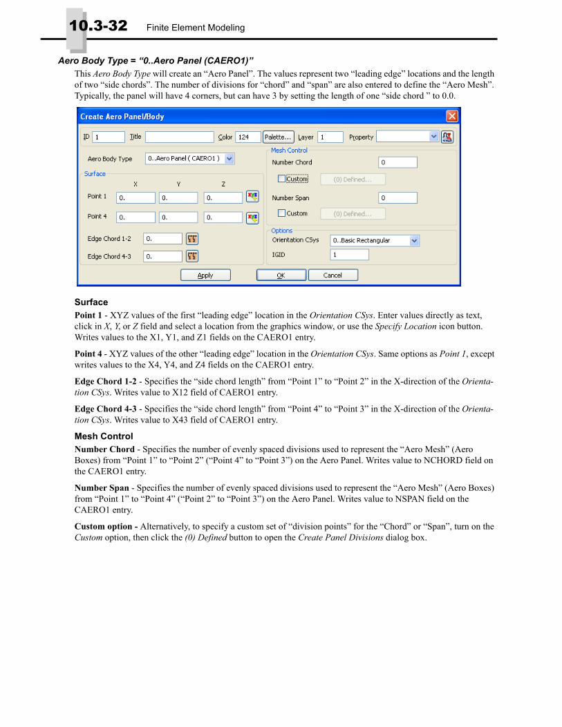
Aero Body Type = “0..Aero Panel (CAERO1)”This Aero Body Type will create an “Aero Panel”. The values represent two “leading edge” locations and the length of two “side chords”. The number of divisions for “chord” and “span” are also entered to define the “Aero Mesh”. Typically, the panel will have 4 corners, but can have 3 by setting the length of one “side chord ” to 0.0.
SurfacePoint 1 - XYZ values of the first “leading edge” location in the Orientation CSys. Enter values directly as text, click in X, Y, or Z field and select a location from the graphics window, or use the Specify Location icon button. Writes values to the X1, Y1, and Z1 fields on the CAERO1 entry.
Point 4 - XYZ values of the other “leading edge” location in the Orientation CSys. Same options as Point 1, except writes values to the X4, Y4, and Z4 fields on the CAERO1 entry.
Edge Chord 1-2 - Specifies the “side chord length” from “Point 1” to “Point 2” in the X-direction of the Orienta-tion CSys. Writes value to X12 field of CAERO1 entry.
Edge Chord 4-3 - Specifies the “side chord length” from “Point 4” to “Point 3” in the X-direction of the Orienta-tion CSys. Writes value to X43 field of CAERO1 entry.
Mesh ControlNumber Chord - Specifies the number of evenly spaced divisions used to represent the “Aero Mesh” (Aero Boxes) from “Point 1” to “Point 2” (“Point 4” to “Point 3”) on the Aero Panel. Writes value to NCHORD field on the CAERO1 entry.
Number Span - Specifies the number of evenly spaced divisions used to represent the “Aero Mesh” (Aero Boxes) from “Point 1” to “Point 4” (“Point 2” to “Point 3”) on the Aero Panel. Writes value to NSPAN field on the CAERO1 entry.
Custom option - Alternatively, to specify a custom set of “division points” for the “Chord” or “Span”, turn on the Custom option, then click the (0) Defined button to open the Create Panel Divisions dialog box.

Model, Aeroelasticity, Panel/Body... 10.3-33
When Division Spacing is set to “Custom”, enter text values directly into the Location field or click the Specify Location icon button to select from the graphics window. Values MUST be between 0.0 and 1.0 and the list MUST include 0.0 and 1.0 to create a valid aero mesh.
Click the Add button to add the current value in Location to the list of values.
Once a value is in the list, it can ben highlighted and the loca-tion will be shown in the graphics window. Click Update but-ton to change a highlighted value to the value currently in the Location field or click Delete button to remove the value from the list. The Reset button can be used to clear all values from the list.
The Copy button can be used to copy the “custom” panel divi-sion list from another Aero Panel/Body in the current model.
The Copy to Clipboard and Paste from Clipboard icon but-tons can be used to copy/paste the current list of values to/from the clipboard.
The Apply button will show the current divisions on the Aero Panel in the graphics window.
When Division Spacing is set to “Bias”, enter a Number, choose a type of Bias (“Bias Equal”, “Bias at Start”, “Bias at End”, “Bias at Center”, or “Bias at Both Ends”) and a enter a Bias Factor (if needed). Once these parameters have been specified, click the Add button in the listing section to add values.
When “Custom” is used for Number Chord, an AEFACT entry will be written to Nastran and the ID of the AEFACT will be referenced by the LCHORD field on the CAERO1. When “Custom” is used for Number Span, the AEFACT is referenced by the LSPAN field of the CAERO1.
Copy to Clipboard Paste from Clipboard

10.3-34 Finite Element Modeling
Some example Aero Panels - Point 1 at (0.0, 0.0, 0.0), Point 4 at (2.0, 10.0, 0.0), Edge Chord 1-2 = 5, Edge Chord 4-3 = 3, Orientation CSys = Basic Rectangular:
Aero Body Type = “1..Aero Body (CAERO2)”This Aero Body Type will create an “Aero Slender/Interference Body”. The values required are a location for the start of the body and the length of the body. The number of divisions for “Slender Body” is also entered to define the “Aero Mesh”. Additionally, a value for the number “Interference Body” divisions needs to be entered.
Only the divisions along the length of the “Slender/Interference Body” are specified using this dialog box. The val-ues for the “Slender Body Radius”, “Interference Body Radius”, and the “Theta Arrays” are defined using the Aero Property with Type set to “Aero Body (PAERO2)”.
SurfacePoint 1 - XYZ values of the first start of the Slender/Interference Body in the Orientation CSys. Enter values directly as text, click in X, Y, or Z field and select a location from the graphics window, or use the Specify Location icon button. Writes values to the X1, Y1, and Z1 fields on the CAERO2 entry.
Edge Chord 1-2 - Specifies the “side chord length” from “Point 1” to “Point 2” in the X-direction of the Orienta-tion CSys. Writes value to X12 field of CAERO2 entry.
Mesh ControlNumber Body Elements - Specifies the number of evenly spaced divisions used to represent the “Aero Mesh” (Aero Boxes) on the “Slender Body” from “Point 1” to “Point 2” on the “Slender Body”. Writes value to NSB field on the CAERO2 entry.
Number Interference Elements - Specifies the number of evenly spaced divisions used to represent the “Interfer-ence Body” from “Point 1” to “Point 2”. Writes value to NINT field on the CAERO2 entry.
Custom option - Alternatively, to specify a custom set of “division points” along the length of the “Slender Body” or “Interference Body”, turn on the Custom option, then click the (0) Defined button to open the Create Panel Divi-
Number Chord = 4, Number Span = 8 Number Chord (Custom) = 4, Bias at Start, BF = 4Number Span (Custom) = 8, Bias at Both Ends, BF = 2

Model, Aeroelasticity, Property... 10.3-35
sions dialog box. For more information on using the Create Panel Divisions dialog box, see the “Custom option” portion of the Aero Body Type = “0..Aero Panel (CAERO1)” section above.
When “Custom” is used for Number Body Elements, an AEFACT entry will be written to Nastran and the ID of the AEFACT will be referenced by the LSB field on the CAERO2. When “Custom” is used for Number Interference Elements, the AEFACT is referenced by the LINT field of the CAERO2.
Model, Aeroelasticity, Property... ...creates an Aero Property for an Aero Panel or an Aero Body (Slender Body and/or Interference Body). The dia-log box changes depending on what is specified for Type. When Type is set to “Aero Panel (PAERO1)”, then FEMAP is making a “Aero Panel” property, which will be written to Nastran as a PAERO1 entry. Other than ID, Title, Color, and Layer, there is nothing else to enter for an “Aero Panel” property.
When Type is set to “Aero Body (PAERO2)”, then FEMAP is making a “Slender/Interference Body” property, which will be written to Nastran as a PAERO2 entry. Along with the ID, Title, Color, and Layer fields, there are several other values which many be entered and effect the display and behavior of all Aero Body entities which ref-erence a particular Aero Property. These additional options are described in greater detail below.
CommonReference Radius - Is the reference half-width of “Slender Body” and the half-width of the constant width “Inter-ference Tube. Writes the WIDTH entry to the PAERO2 entry.
Aspect Ratio (h/w) - Aspect Ratio of interference tube (height/width). Writes the AR field to the PAERO2 entry.
Number of Body Elements = 6Number of Interference Elements = 6Reference Radius on Aero Property = 2.5Shown in Wireframe Display Mode
Number of Body Elements = 8Number of Interference Elements = 8Reference Radius on Aero Property = 2.5Slender Body Division Radius list on Aero Property0, 1.111, 1.778, 2, 2, 2, 2.5, 2.5, 2.5

10.3-36 Finite Element Modeling
Slender Body PropertiesOrientation - Specifies the type of motion allowed for bodies. The selected direction (Z, Y, or ZY) is in the speci-fied “aerodynamic coordinate system” for the analysis. Writes “Z”. “Y”, or “ZY” to the ORIENT field of the PAERO2 entry.
Slender Body Division Radius - When on, allows you to enter a list of slender body half-widths at the “end points” of the slender body “Aero Elements”. When off, the half-width of the entire slender body is specified by the Reference Radius value in the Common section. Click the Custom List... button to enter values in the Create Cus-tom Cross Section dialog box. See Create Custom Cross Section dialog box section below for more details.
Interference Body Division Radius - When on, allows you to enter a list of slender body half-widths at the “end points” of the interference body “Aero Elements”. Click the Custom List... button to enter values in the Create Cus-tom Cross Section dialog box. See Create Custom Cross Section dialog box section below for more details.
Note: In FEMAP, the “aerodynamic coordinate system” is defined using the Analysis Set Manager (“Model, Analysis” command). When Analysis Type is set to “25..Static Aeroelasticity”, the aero-dynamic coordinate system is specified by the Aerodynamic CSys drop-down in the NASTRAN Aerodynamic Data (AEROS) dialog box. When Analysis Type is set to “26..Aerodynamic Flutter”, it is specified by the Aerodynamic CSys drop-down in the NASTRAN Aerodynamic Data (AEROx, MKAEROx) dialog box.
Note: The number of Radius values entered for the Aero Property MUST correspond to the number of divisions specified Number Body Elements (constant or custom) on the Aero Body. Therefore, if there are 8 constant divisions, you need to enter 9 Radius values (1 value for the “start” of the aero body, 7 for each “division location”, and 1 value for the “end”).
Note: The number of Radius values entered for the Aero Property MUST correspond to the number of divisions specified Number Interference Elements (constant or custom) on the Aero Body. There-fore, if there are 8 constant divisions, you need to enter 9 Radius values (1 value for the “start” of the aero body, 7 for each “division location”, and 1 value for the “end”).
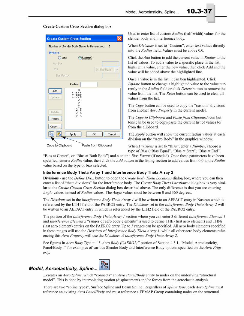
Model, Aeroelasticity, Spline... 10.3-37
Create Custom Cross Section dialog box
Used to enter list of custom Radius (half-width) values for the slender body and interference body.
When Divisions is set to “Custom”, enter text values directly into the Radius field. Values must be above 0.0.
Click the Add button to add the current value in Radius to the list of values. To add a value to a specific place in the list, highlight a value, enter the new value, then click Add and the value will be added above the highlighted line.
Once a value is in the list, it can ben highlighted. Click Update button to change a highlighted value to the value cur-rently in the Radius field or click Delete button to remove the value from the list. The Reset button can be used to clear all values from the list.
The Copy button can be used to copy the “custom” divisions from another Aero Property in the current model.
The Copy to Clipboard and Paste from Clipboard icon but-tons can be used to copy/paste the current list of values to/from the clipboard.
The Apply button will show the current radius values at each division on the “Aero Body” in the graphics window.
When Divisions is set to “Bias”, enter a Number, choose a type of Bias (“Bias Equal”, “Bias at Start”, “Bias at End”,
“Bias at Center”, or “Bias at Both Ends”) and a enter a Bias Factor (if needed). Once these parameters have been specified, enter a Radius value, then click the Add button in the listing section to add values from 0.0 to the Radius value based on the type of bias selected.
Interference Body Theta Array 1 and Interference Body Theta Array 2Divisions - use the Define Div... button to open the Create Body Theta Locations dialog box, where you can then enter a list of “theta divisions” for the interference body. The Create Body Theta Locations dialog box is very simi-lar to the Create Custom Cross Section dialog box described above. The only difference is that you are entering Angle values instead of Radius values. The Angle values must be between 0 and 360 degrees.
The Divisions set in the Interference Body Theta Array 1 will be written to an AEFACT entry in Nastran which is referenced by the LTH1 field of the PAERO2 entry. The Divisions set in the Interference Body Theta Array 2 will be written to an AEFACT entry in which is referenced by the LTH2 field of the PAERO2 entry.
The portion of the Interference Body Theta Array 1 section where you can enter 3 different Interference Element 1 and Interference Element 2 “ranges of aero body elements” is used to define THIi (first aero element) and THNi (last aero element) entries on the PAERO2 entry. Up to 3 ranges can be specified. All aero body elements specified in these ranges will use the Divisions of Interference Body Theta Array 1, while all other aero body elements refer-encing this Aero Property will use the Divisions of Interference Body Theta Array 2.
See figures in Aero Body Type = “1..Aero Body (CAERO2)” portion of Section 4.5.1, “Model, Aeroelasticity, Panel/Body...” for examples of various Slender Body and Interference Body options specified on the Aero Prop-erty.
Model, Aeroelasticity, Spline... ...creates an Aero Spline, which “connects” an Aero Panel/Body entity to nodes on the underlying “structural model”. This is done by interpolating motion (displacement) and/or forces from the aeroelastic analysis.
There are two “spline types”, Surface Spline and Beam Spline. Regardless of Spline Type, each Aero Spline must reference an existing Aero Panel/Body and must reference a FEMAP Group containing nodes on the structural
Copy to Clipboard Paste from Clipboard

10.3-38 Finite Element Modeling
model. Also, at least 2 “aerodynamic points” (aero elements/aero boxes) from the referenced Aero Panel/Body must be selected.
The ID, Title, Color, and Layer fields are common to both Spline Types.
TypeSpline Type - choose between “0..Surface Spline” and “1..Beam Spline”. When using “0..Surface Spline” the Aero Spline will be written as a SPLINE1 entry to Nastran and additional entries for the SPLINE1 may be specified in the Surface Spline section. A “1..Beam Spline” will be written as SPLINE2 and additional entries for SPLINE2 may be specified in the Beam Spline section.
SplineCAERO ID - used to enter the ID of an existing Aero Panel/Body entity. The ID may be entered in manually or an Aero Panel/Body may be chosen from the graphics window. The Show When Selected icon button will highlight the specified Aero Panel/Body in the graphics window, while the Select Aero Panel icon button will allow you to choose an Aero Panel/Body from a list. This value will be written to the CAERO field on the SPLINEi entry.
Structural Grid GroupID - used to specify the ID of a Group in FEMAP containing nodes on the structural model. The Show When Selected icon button will highlight nodes in the group in the graphics window. The Quick Group icon button will open the Quick Group dialog box, which can be used to create a new Group or edit an existing one.
In the Quick Group dialog box, click New Group to create a new group.
Highlight the new group or an existing one, then click Edit Group to Add, Remove, or Exclude nodes to/from the group. Since these groups only need to contain nodes, the only thing which can be selected using this dialog box is nodes.
You can rename any group by highlighting it in the list, then clicking Rename.
To “Show” the highlighted group in the graphics window, click Show. When done looking at the Group, press Hide. Click Done to exit the Quick Group dialog box.
Model, Aeroelasticity, Spline... 10.3-39
The selected group will be written to as a SET1 entry to Nastran which is referenced by the SETG field of the SPLINEi entry.
Aerodynamic PointsBox1 - enter the ID or select an aero element (aero box) from the screen to be the first aero element in a “range of aero elements” where motions (displacements) will be interpolated. Click the Select Aero Mesh for Aero Spline icon button to bring up a dialog box which may make graphical selection of the aero element easier. This value will be written to the BOX1 field on the SPLINE1 and to the ID1 field of the SPLINE2 entry.
Box2 - similar to Box1, but is last aero element in a “range of aero elements” where motions (displacements) will be interpolated. This value will be written to the BOX2 field on the SPLINE1 entry and to the ID2 field of the SPLINE2 entry .
All Boxes button - when chosen, places the aero element with the lowest ID on the referenced Aero Panel/Body into the Box1 field and the one with the highest ID in the Box2 field.
UsageDetermines if the Aero Spline applies to Force transformation, Displacement transformation, or Both. Writes FORCE, DISP, or BOTH to the USAGE field for the SPLINEi entry.
Surface SplineThese options are only used for Aero Spline entities with Spline Type set to “0..Surface Spline” and will be written to the appropriate field on the SPLINE1 entry.
Attachment Flexibility - specifies the linear attachment flexibility. Value written to the DZ field on SPLINE1
Nelem- number of structural elements along the local spline x-axis if using “2..FPS” option for Spline Fit Method. Value written to NELEM field on SPLINE1
Melem - number of structural elements along the local spline y-axis if using “2..FPS” option for Spline Fit Method. Value written to MELEM field on SPLINE1
Spline Fit Method - designates which spline fit method to use for the Aero Spline. Choose between 0..IPS (Harder-Desmarais Infinite Plate Spline), 1..TPS (Thin Plate Spline), or 2..FPS (Finite Plate Spline). Writes IPS, TPS, or FPS to METH field on SPLINE1
Beam SplineThese options are only used for Aero Spline entities with Spline Type set to “1..Beam Spline” and will be written to the appropriate field on the SPLINE2 entry.
Attachment Flexibility - specifies the linear attachment flexibility. Value written to the DZ field on SPLINE2
Torsional Flexibility - specifies the torsional flexibility ratio (EI/GJ). Value written to DTOR field on SPLINE2. Use 1.0 for “aero bodies”.
X Rot Flex - specifies the rotational attachment flexibility about the spline’s x-axis (in-plane bending rotations) is specified in Y CSys. Not used for “aero bodies”, only “aero panels”. Value written to DTHX field on SPLINE2.
Y Rot Flex - specifies the rotational attachment flexibility about the spline’s y-axis (torsion) is specified in Y CSys. May be used for “slope” of “aero bodies”. Value written to DTHY field on SPLINE2.
Y Csys - Rectangular coordinate system where the y-axis defines the axis of the spline. Not used for “aero bodies”, only “aero panels”. Only rectangular coordinate systems will be available for selection. Value written to DCID field on SPLINE2.
For display purposes, each Aero Spline will be drawn “on top” of the selected “aero mesh” of the referenced Aero Panel/Body. In addition, straight “connection lines” will be drawn from each node in the referenced Structural Grid Group to the centroid of the referenced Aero Panel/Body.
Note: The values for Attachment Flexibility, X Rot Flex, and Y Rot Flex are used for smoothing. Flexibil-ity values of 0.0 in these fields imply rigid attachment (i.e., no smoothing). Negative values for X Rot Flex and Y Rot Flex imply infinity, therefore, no attachment.

10.3-40 Finite Element Modeling
For example, an “aero panel” and an “aero body” are shown on the left. The corresponding Aero Splines for these Aero Panel/Body entities are shown on the right.
Model, Aeroelasticity, Control Surface... ...creates an Aero Control Surface, which is used to specify an aerodynamic control surface. Each Aero Control Surface uses ranges of aero elements on “aero panels” (not “aero bodies”) to represent the aerodynamic control sur-face. Two ranges of aero elements may be specified on each Aero Control Surface, with each “control surface” range able to use a different “hinge orientation coordinate system”.
The ID, Title, Color, and Layer fields work as the do for other entities.
UsageThese options allow you to create an easy to recognize label which will be written to the Nastran input file and effect how each Aero Control Surface is used in the aeroelastic analysis.
Label - specifies the name of the control surface. Limited to 7 characters. Text written to the LABEL field on AESURF.
1 “aero panel” and 1 “aero body” Same “aero panel” and “aero body”shown with corresponding aero splines

Model, Aeroelasticity, Control Surface... 10.3-41
Linear Downwash/No Linear Downwash - specifies if “Linear DownWash” is computed as part of the database (Linear Downwash) or if the effects of the control surface must be entered by the user directly (No Linear Down-wash). Writes LDW or NOLDW to the LDW field on AESURF.
Effectiveness - specifies the control surface effectiveness, which cause forces to be modified by this value (i.e., to achieve 40% reduction of effectiveness, specify this value as 0.6). Value written to EFF field on AESURF entry.
Ref Chord Length - specifies the reference chord length of the control surface. Value written to CREFC field on AESURF entry.
Ref Surface Area - specifies the reference surface area of the control surface. Value written to CREFS field on AESURF entry.
Deflection LimitsSpecifies the Lower and Upper deflection limits for the control surface in radians. Values written to PLLIM and PULIM fields on AESURF entry.
Hinge Moment LimitsSpecifies the Lower and Upper hinge moment limits for the control surface in force-length units. Values written to HMLLIM and HMULIM fields on AESURF entry.
Deflection Limits vs PressureAllows you to choose functions to specify Lower and Upper deflection limits for the control surface as a function of dynamic pressure. Functions written as TABLED1 entries to Nastran then referenced by TQLLIM and TQULIM fields on AESURF entry.
Control Surface 1 and Control Surface 2Specify a rectangular coordinate system as the Hinge Orientation CSys (writes CIDi to AESURF entry), then click the Aero Mesh... button to choose “aero panel elements” using a typical Entity Selection dialog box. The selected “aero mesh” in each section will be written as an AELIST to Nastran, then referenced by the corresponding ALIDi field(s) on the AESURF entry
Aero Control Surfaces are displayed “on top” of the “aero panel elements”.
A “complete” Aero model shown below with Aero Control Surfaces:
RUDDER (single control surface on Aero Control Surface entity)
AILERON (both defined on same Aero Control Surface entity)

10.3-42 Finite Element Modeling
Static Aeroelasticity AnalysisNX and MSC/MD Nastran have the ability to perform Static Aeroelasticity analysis using Solution Sequence 144 (SOL 144).
Specific Solution 144 dialog boxes will appear in the Analysis Set Manager when the Analysis Type has been set to 25..Static Aeroelasticity. The NASTRAN Aerodynamic Data (AEROS) dialog box allows you to enter basic parame-ters for static aeroelasticity and an optional conversion factor PARAM used for all subcases. On the other hand, the NASTRAN Aeroelastic Trim Parameters dialog box contains a number of “Trim Parameters”, which may be speci-fied in the “Master Requests and Conditions” for an analysis with no subcases or specified individually for each subcase.
AEROF and APRES will be written to case control to request results from static aeroelastic analysis.
NASTRAN Aerodynamic Data (AEROS)
Aerodynamic Physical DataAerodynamic CSys - specifies the aerodynamic coordinate system. Must be a rectangular coordinate system. Flow is in the +X direction. Value written to the ACSID field of the AEROS entry.
Ref CSys - specifies the reference coordinate system. Must be a rectangular coordinate system. All AESTAT degrees-of-freedom defining trim variables will be defined in this coordinate system. Value written to the RCSID field of the AEROS entry.
Chord Length - specifies reference chord length. Value written to the REFC field of the AEROS entry.
Span - specifies reference span. Value written to the REFB field of the AEROS entry.
Wing Area - specifies reference wing area. Value written to the REFS field of the AEROS entry.
PARAM, AUNITS - writes PARAM, AUNITS to the Nastran input file with the specified value. This parameter is used to convert accelerations specified in units of gravity on the TRIM entries to units of distance per time squared.
SymmetryXZ - specifies the symmetry “key” for the x-z plane of the Aerodynamic CSys. Based on option selected for XZ, writes an integer to the SYMXZ (Symmetry = +1, No Symmetry = 0, Anti-Symmetry = -1).
XY - specifies the symmetry “key” for the x-y plane of the Aerodynamic CSys, which can be used to simulate “ground effects”. Based on option selected for XY, writes an integer to the SYMXY (Symmetry = -1, No Symmetry = 0, Anti-Symmetry = +1).
NASTRAN Aeroelastic Trim ParametersThe Enable Trim check box may be used to toggle the options set in the NASTRAN Aeroelastic Trim Parameters dialog on/off in the Master case and for each subcase.
The Trim Parameters in the upper portion of the dialog box are used to define values on the TRIM bulk data entry.
Mach Number - specifies the mach number. Value written to the MACH field of the TRIM entry.
Dynamic Pressure - specifies a value for dynamic pressure. Value written to the Q field of the TRIM entry.
Rigid Trim Analysis - specifies if trim analysis is rigid. When “on” a value of 0.0 is written to the AEQR field of the TRIM entry. When “off”, a value of 1.0 is written to the AEQR field of the TRIM entry.

Aerodynamic Flutter Analysis 10.3-43
The Trim Parameters in the lower portion of the dialog box write AESTAT and/or TRIM entries using values entered for various “Trim Variables” in the list.
When set to Rigid Body Motion:
a. Select from the list of "Standard Labels Defining Rigid Body Motions" on the AESTAT (ANGLEA, SIDES, ROLL, PITCH, YAW, URDD1, URDD2, URDD3, URDD4, URDD5, and URDD6)
b. Select a Usage (1..Free or 2..Fixed). If 2..Fixed, enter a magnitude as well (UXi value on TRIM entry).
c. Click Add to add the “Trim Variable” to the list in the lower portion of the dialog box.
When set to Control Surfaces:
a. Select from the list of Aero Control Surfaces in your model, then follow steps b and c above.
To update a “Trim Variable”, highlight one in the list, set the appropriate values, then click Update. The Delete but-ton is used to delete a single highlighted “Trim Variable” from the list, while Reset will delete all “Trim Variables” from the list.
Aerodynamic Flutter AnalysisNX and MSC/MD Nastran have the ability to perform Aerodynamic Flutter analysis using Solution Sequence 145 (SOL 145).
Specific Solution 145 dialog boxes will appear in the Analysis Set Manager when the Analysis Type has been set to 26..Aerodynamic Flutter. The NASTRAN Aerodynamic Data (AEROx, MKAEROx) dialog box allows you to enter basic parameters for unsteady aerodynamics, a table of Mach numbers vs. Reduced frequencies, and some addi-tional dynamic analysis information. On the other hand, the NASTRAN Flutter Parameters dialog box contains a number of “Flutter Parameters”, which may be specified in the “Master Requests and Conditions” for an analysis with no subcases or specified individually for each subcase.
The standard NASTRAN Modal Analysis dialog box is also used to setup a Flutter analysis. See Section 8.7.1.9, “Modal Analysis” for more information about the options available in this dialog box.
When using the PK method, results from the Flutter Summery Table will be imported into FEMAP as functions.
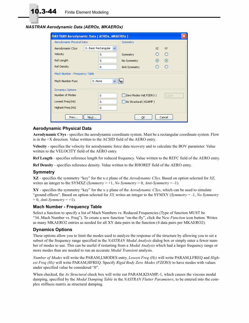
10.3-44 Finite Element Modeling
NASTRAN Aerodynamic Data (AEROx, MKAEROx)
Aerodynamic Physical DataAerodynamic CSys - specifies the aerodynamic coordinate system. Must be a rectangular coordinate system. Flow is in the +X direction. Value written to the ACSID field of the AERO entry.
Velocity - specifies the velocity for aerodynamic force data recovery and to calculate the BOV parameter. Value written to the VELOCITY field of the AERO entry.
Ref Length - specifies reference length for reduced frequency. Value written to the REFC field of the AERO entry.
Ref Density - specifies reference density. Value written to the RHOREF field of the AERO entry.
SymmetryXZ - specifies the symmetry “key” for the x-z plane of the Aerodynamic CSys. Based on option selected for XZ, writes an integer to the SYMXZ (Symmetry = +1, No Symmetry = 0, Anti-Symmetry = -1).
XY - specifies the symmetry “key” for the x-y plane of the Aerodynamic CSys, which can be used to simulate “ground effects”. Based on option selected for XY, writes an integer to the SYMXY (Symmetry = -1, No Symmetry = 0, Anti-Symmetry = +1).
Mach Number - Frequency TableSelect a function to specify a list of Mach Numbers vs. Reduced Frequencies (Type of function MUST be “34..Mach Number vs. Freq”). To create a new function “on-the-fly”, click the New Function icon button. Writes as many MKAERO2 entries as needed for all XY data pairs in the function (4 data pairs per MKAERO2).
Dynamics OptionsThese options allow you to limit the modes used to analyze the response of the structure by allowing you to set a subset of the frequency range specified in the NASTRAN Modal Analysis dialog box or simply enter a fewer num-ber of modes to use. This can be useful if restarting from a Modal Analysis which had a larger frequency range or more modes than are needed to run an accurate Modal Transient analysis.
Number of Modes will write the PARAM,LMODES entry, Lowest Freq (Hz) will write PARAM,LFREQ and High-est Freq (Hz) will write PARAM,HFREQ. Specify Rigid Body Zero Modes (FZERO) to have modes with values under specified value be considered “0”.
When checked, the As Structural check box will write out PARAM,KDAMP,-1, which causes the viscous modal damping, specified by the Modal Damping Table in the NASTRAN Flutter Parameters, to be entered into the com-plex stiffness matrix as structural damping.
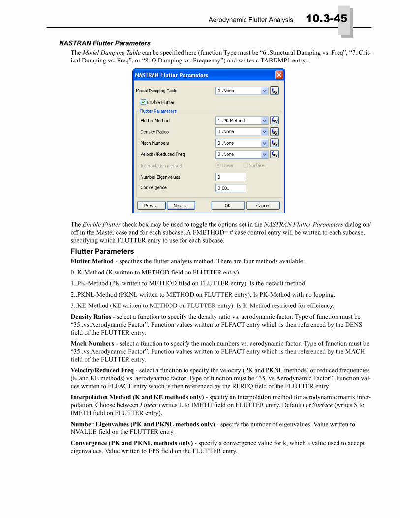
Aerodynamic Flutter Analysis 10.3-45
NASTRAN Flutter ParametersThe Model Damping Table can be specified here (function Type must be “6..Structural Damping vs. Freq”, “7..Crit-ical Damping vs. Freq”, or “8..Q Damping vs. Frequency”) and writes a TABDMP1 entry..
The Enable Flutter check box may be used to toggle the options set in the NASTRAN Flutter Parameters dialog on/off in the Master case and for each subcase. A FMETHOD= # case control entry will be written to each subcase, specifying which FLUTTER entry to use for each subcase.
Flutter ParametersFlutter Method - specifies the flutter analysis method. There are four methods available:
0..K-Method (K written to METHOD field on FLUTTER entry)
1..PK-Method (PK written to METHOD filed on FLUTTER entry). Is the default method.
2..PKNL-Method (PKNL written to METHOD on FLUTTER entry). Is PK-Method with no looping.
3..KE-Method (KE written to METHOD on FLUTTER entry). Is K-Method restricted for efficiency.
Density Ratios - select a function to specify the density ratio vs. aerodynamic factor. Type of function must be “35..vs.Aerodynamic Factor”. Function values written to FLFACT entry which is then referenced by the DENS field of the FLUTTER entry.
Mach Numbers - select a function to specify the mach numbers vs. aerodynamic factor. Type of function must be “35..vs.Aerodynamic Factor”. Function values written to FLFACT entry which is then referenced by the MACH field of the FLUTTER entry.
Velocity/Reduced Freq - select a function to specify the velocity (PK and PKNL methods) or reduced frequencies (K and KE methods) vs. aerodynamic factor. Type of function must be “35..vs.Aerodynamic Factor”. Function val-ues written to FLFACT entry which is then referenced by the RFREQ field of the FLUTTER entry.
Interpolation Method (K and KE methods only) - specify an interpolation method for aerodynamic matrix inter-polation. Choose between Linear (writes L to IMETH field on FLUTTER entry. Default) or Surface (writes S to IMETH field on FLUTTER entry).
Number Eigenvalues (PK and PKNL methods only) - specify the number of eigenvalues. Value written to NVALUE field on the FLUTTER entry.
Convergence (PK and PKNL methods only) - specify a convergence value for k, which a value used to accept eigenvalues. Value written to EPS field on the FLUTTER entry.

10.3-46 Finite Element Modeling
Loads and Constraints• Updated Model, Load, From Freebody command to allow selection of a Freebody entity currently in the model.
• Added Map Tolerance field for Model, Load, Map Output from Model command and in Data Surface editor
Map Tolerance - When a “Target” location is projected onto the “Source” data surface and the distance to a discrete data point is less than the tolerance, the “Source” value of the "coincident" location is directly mapped to the “Tar-get” without interpolation. If multiple nodes fall within this tolerance, then the first one encountered numerically will be directly mapped. Default value is the "Merge Tolerance" of the "Target” model.
• Enhanced Model, Constraint, Expand command.
Connections (Connection Region, Properties, and Connectors)• Added Activation Distance section to Penetration section on the NEiNastran tab. Allows you to specify a value
(real or AUTO) for MAXAD or specify values for MAXNAD and/or MAXRAD)
• Added Friction section to LS-DYNA tab to restore ability to set these values for LS-Dyna contact.
• Updated Fluid Regions to not use the PLANE1, PLANE2, RMAX, FMEXACT inputs when NEi Nastran is default solver.
Groups and Layers• Added on Group, Coord Sys, On Property to add coordinate systems on a Property to a group and Group, Coord
Sys, on CSys to add coordinate systems referenced by selected coordinate systems to a group.
• Enhanced Group, Operations, Add Related Entities to now add Coordinate Systems referenced on Properties and coordinate systems referenced by other coordinate systems to a group.
Views• Added on View, Align by, Surface to align the view normal to a selected surface and View, Align by, Normal to
Plane to align view normal to a specified plane.
• Added Aero Panel, Aero Mesh, Aero Interference, Aero Splines, and Aero Control Surfaces to Labels, Entities and Color Category of View, Options.
• Added Preview option to Tools and View Style Category of View, Options. Controls the size of the “marker” shown in the graphics window when using the Preview button to preview the location of a coordinate.
• Added Freebody, Freebody Node Markers, Freebody Vectors, Freebody Total Force, Freebody Total Moment, Freebody Nodal Force, and Freebody Nodal Moment to PostProcessing Category of View, Options.
• Added Max Only and Min Only options to the Label Mode of the Contour/Criteria Style option in the PostPro-cessing Category of View, Options.
• Only tabs of entity types which currently exist in the model will be displayed in the View, Visibility dialog box.
Output and Post-Processing• Freebody display has been enhanced and is now managed via the Freeboy tool in the PostProcessing Toolbox.
• Added “Select By Vector” options for Nodal and Elemental output in Model, Output, Forced Response. This allows you to limit the amount of output created by this command.
Geometry InterfacesThe following FEMAP interfaces have been updated to support newer geometry formats:
FEMAP Interface Latest Supported VersionParasolid Parasolid 24.0Solid Edge Solid Edge with Synchronous Technology 4NX NX 8.0
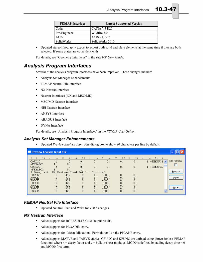
Analysis Program Interfaces 10.3-47
• Updated stereolithography export to export both solid and plate elements at the same time if they are both selected. If some plates are coincident with
For details, see “Geometry Interfaces” in the FEMAP User Guide.
Analysis Program InterfacesSeveral of the analysis program interfaces have been improved. These changes include:
• Analysis Set Manager Enhancements
• FEMAP Neutral File Interface
• NX Nastran Interface
• Nastran Interfaces (NX and MSC/MD)
• MSC/MD Nastran Interface
• NEi Nastran Interface
• ANSYS Interface
• ABAQUS Interface
• DYNA Interface
For details, see “Analysis Program Interfaces” in the FEMAP User Guide.
Analysis Set Manager Enhancements• Updated Preview Analysis Input File dialog box to show 80 characters per line by default.
FEMAP Neutral File Interface• Updated Neutral Read and Write for v10.3 changes
NX Nastran Interface• Added support for BGRESULTS Glue Output results.
• Added support for PLOADE1 entry.
• Added support for “Mean Dilatational Formulation” on the PPLANE entry.
• Added support MATVE and TABVE entries. GFUNC and KFUNC are defined using dimensionless FEMAP functions where x = decay factor and y = bulk or shear modulus. MOD0 is defined by adding decay time = 0 and MOD0 first term.
Catia CATIA V5 R20Pro/Engineer Wildfire 5.0ACIS ACIS 21, SP3SolidWorks SolidWorks 2010
FEMAP Interface Latest Supported Version
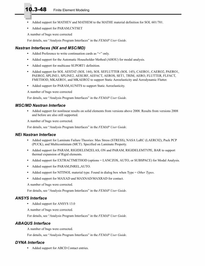
10.3-48 Finite Element Modeling
• Added support for MATHEV and MATHEM to the MATHE material definition for SOL 601/701.
• Added support for PARAM,CNTSET
A number of bugs were corrected
For details, see “Analysis Program Interfaces” in the FEMAP User Guide.
Nastran Interfaces (NX and MSC/MD)• Added Preference to write continuation cards as “+” only.
• Added support for the Automatic Householder Method (AHOU) for modal analysis.
• Added support for multicase SUPORT1 definition.
• Added support for SOL AESTAT (SOL 144), SOL SEFLUTTER (SOL 145), CAERO1, CAERO2, PAERO1, PAERO2, SPLINE1, SPLINE2, AESURF, AEFACT, AEROS, SET1, TRIM, AERO, FLUTTER, FLFACT, FMETHOD, MKAERO1, and MKAERO2 to support Static Aeroelasticity and Aerodynamic Flutter.
• Added support for PARAM,AUNITS to support Static Aeroelasticity.
A number of bugs were corrected
For details, see “Analysis Program Interfaces” in the FEMAP User Guide.
MSC/MD Nastran Interface• Added support for nonlinear results on solid elements from versions above 2008. Results from versions 2008
and before are also still supported.
A number of bugs were corrected.
For details, see “Analysis Program Interfaces” in the FEMAP User Guide.
NEi Nastran Interface• Added support for Laminate Failure Theories: Max Stress (STRESS), NASA LaRC (LAERC02), Puck PCP
(PUCK), and Multicontinium (MCT). Specified on Laminate Property.
• Added support for PARAM, RIGIDELEM2ELAS, ON and PARAM, RIGIDELEMTYPE, BAR to support thermal expansion of Rigid elements.
• Added support for EXTRACTMETHOD (options = LANCZOS, AUTO, or SUBSPACE) for Modal Analysis.
• Added support for PARAM,INREL,AUTO.
• Added support for NITINOL material type. Found in dialog box when Type = Other Types.
• Added support for MAXAD and MAXNAD/MAXRAD for contact.
A number of bugs were corrected.
For details, see “Analysis Program Interfaces” in the FEMAP User Guide.
ANSYS Interface• Added support for ANSYS 13.0
A number of bugs were corrected.
For details, see “Analysis Program Interfaces” in the FEMAP User Guide.
ABAQUS InterfaceA number of bugs were corrected.
For details, see “Analysis Program Interfaces” in the FEMAP User Guide.
DYNA Interface• Added support for ABCD Contact entries.

Tools 10.3-49
A number of bugs were corrected.
For details, see “Analysis Program Interfaces” in the FEMAP User Guide.
Tools• Added Color, Next ID, and Inc values for Aero Panel, Aero Property, Aero Spline, and Aero Surface to Tools,
Parameters.
• Added ability to determined surface area of “combined surfaces” to Tools, Measure, Surface Area.
• Added “Skew” element quality check to Tools, Check, Element Quality command.
Skew measures internal angular deviation of a face using the edge bisector method. This check matches results reported by NX Nastran. Only this command will return Skew results for faces of supported solid elements.
For Triangular elements and element faces, Skew measures internal angle and reports minimum for all angles of 2-D (a1, a2 & a3 in figure below) and all angles of all faces of supported 3-D type elements.
For Quadrilateral elements and element faces, Skew test for quadrilateral faces reports minimum angle between face edge bisectors ( a1 & a2 in figure below ). Minimum for all faces is reported for supported 3-D elements.
OLE/COM APINew API Objects and Attributes• Added Element Quality (feElementQuality) object to the API. Also added AspectRatioOn, TaperOn, Alter-
nateTaperOn, InternalAngleOn, SkewOn, WarpingOn, NastranWarpingOn, TetCollapseOn, JacobianOn, Com-binedOn, ExplicitTimeStepOn, AspectRatioLimit, TaperLimit, AlternateTaperLimit, InternalAngleLimit, SkewLimit, WarpingLimit, NastranWarpingLimit, TetCollapseLimit, JacobianLimit, CombinedLimit, and ExplicitTimeStepLimit to Element Quality Object.
• Added Aero Panel/Body (feAeroPanel) object to the API. Also added color, layer, title, propID, defCSys, nSpan, nChord, iIgid, Pt1, Pt4, dChord12, dChord43, nLspanID, nLchordID, and type attributes to the Aero Panel/Body object.
• Added Aero Property (feAeroProp) object to the API. Also added color, layer, title, pdval, pnval, ap_d_width, ap_d_ar, ap_i_orient, ap_i_lrsb, ap_i_lrib, ap_i_lth1, ap_i_lth2, ap_i_thi1, ap_i_thi2, ap_i_thi3, ap_i_thn1, ap_i_thn2, ap_i_thn3, and type attributes to the Aero Property object.
• Added Aero Spline (feAeroSpline) object to the API. Also added color, layer, title, type, icaero, ibox1, ibox2, isetg, dz, meth, nelem, melem, usage, dtor, cid, dthx, and dthy attributes to the Aero Spline object.
• Added Aero Control Surface (feAeroSurf) object to the API. Also added color, layer, title, csys, csys1, aeid, aeid1, eff, ldw, crefc, crefs, pllim, pulim, hmllim, hmulim, tqllim, tqulim, and label attributes to the Aero Con-trol Surface object.
• Added Freebody (feFreebody) object to the API. Also added title, DisplayMode, Group, CSys, NodeMarker-Color, TotalVectorMode, ShowTotalVec, SumComponents, TotalVecColor, x, y, z, NodalVectorMode, ShowN-odalVec, NodalVecColor, and SumContributions attributes to the Freebody object.
• Added Geometry Preparation and Meshing (feMesher) object to the API. This object has been partially added and is for “Future Use” and should not be used.

10.3-50 Finite Element Modeling
• Added NasAeroOn, NasAeroCsID, NasAeroRefCsID, NasAeroRefLength, NasAeroRefSpan, NasAeroRe-fArea, NasAeroSymXY, NasAeroSymxz, NasAeroAeunit, NasAeroAeunitVal, NasAeroVelo, NasAer-oRefDens, NasAeroMkFuID, vNasAeroFreqKeep, NasAeroModesKeep, NasAerobPARAMfzero, NasAerodPARAMfzero, and NasAeroDampMethod attributes to Analysis Manager (AnalysisMgr)object for Static Aeroelasticity and Aerodynamic Flutter. Also, added NasBulkCntAset for Bulk Data.
• Added NasCaeOn, NasCaeMachNumber, NasCaeDynPressure, NasCaeRigidTrim, NasCaeWrtieTrim, NasC-flOn, NasCflMethod, NasCflDenID, NasCflMachFactID, NasCflRfreqFactID, NasCflFliMethod, NasCflEig, NasCflEps, NasCflWriteFlutter, NasCflSdamp attributes to Analysis Case (AnalysisCase) object for Static Aeroelasticity and Aerodynamic Flutter.
New API Methods• Added NextExistingInSet to Entity API objects
• Added Clear, SetModelDefaults, GetModelDefaults, CheckQuality, GetAspectRatio, AspectRatio, GetTaper, Taper, GetAlternateTaper, AlternateTaper, GetInternalAngle, InternalAngle, GetSkew, Skew, GetWarping, Warping, GetNastranWarping, NastranWarping, GetTetCollapse, TetCollapse, GetJacobian, Jacobian, Get Combined, Combined, GetExplicitTimeStep, and ExplicitTimeStep to Element Quality object.
• Added GetDivisionList, PutDivisionList, SlenderBodyCount, InterferenceBodyCount, PanelSpanCount, Panal-ChordCount, and GetBoxSet to Aero Panel/Body object
• Added GetThetaList, PutThetaList, GetRadiList, PutRadiList, ClearSbList, ClearIbList, ClearTheta1List, and ClearTheta2List to Aero Property object
• Added GetNodeSet and GetBoxSet to Aero Spline object
• Added PutSurfaceSet1, PutSurfaceSet2, GetSurfaceSet1, GetSurfaceSet2, ClearSurfaceSet1, and ClearSurfaceSet2 to Aero Control Surface object
• Added GetElements, SetElements, ClearElements, GetNodes, SetNodes, ClearNodes, CalculateNodalCenter, and CalculateSummation to Freebody object.
• Added Axis and TwoAxis to CSys object
• Added ClearMeshLoc and PointsAsSet to Curve object
• Added FindMappedMeshingCorners, AddMeshPoint, CountMeshPoint, and PointLoops to Surface object
• Added CountCommon, CountNotCommon, HasNotCommon, and NextAfter to Set object
• Added SetMultiGroupListFromSets to View object
• Added IsEmpty to SortSet object
• Added ElementsAsSet2 to Solid object
• Added MapFromModelToSet2 to MapOutput object.
• Added DeleteAnalysisCase to Analysis Case object.
• Added GetList to Group object
New Global Variables• Added Pref_JTFileVersion, Pref_GIFOptimized, and Pref_2DTensorPlotOverride
• Added Pref_RenderXORPicking, Pref_RenderMultiModelMem, Pref_RenderDebugElapsedTime, Pref_DebugAllTime, Pref_DebugOGLErrors, Pref_RenderBlockSize, and Pref_DialogRefresh
• Added Pref_PickMethod, Pref_ConfirmDelete, Pref_ShowMode, Pref_ShowLables, Pref_ShowNormals, and Pref_ShowColor.
• Added Pref_PreserveNextID, Pref_DBOpenSaveWindowsIO, and Pref_DBOpenSaveUnblockedIO
• Added Pref_Prev10TetMesh, Pref_Prev10SurfaceMesh, Pref_ElemQualAspectRatio, Pref_ElemQualTaper, Pref_ElemQualAltTaper, Pref_ElemQualIntAngles, Pref_ElemQualSkew, Pref_ElemQualWarping, Pref_ElemQualNastranWarping, Pref_ElemQualTetCollapse, Pref_ElemQualJacobian, Pref_ElemQualCombined, Pref_ElemQualExplicitTime, Pref_ElemQualAspectRatioVal, Pref_ElemQualTaperVal, Pref_ElemQualAltTaperVal, Pref_ElemQualIntAnglesVal, Pref_ElemQualSkewVal,
Preferences 10.3-51
Pref_ElemQualWarpingVal, Pref_ElemQualNastranWarpingVal, Pref_ElemQualTetCollapseVal, Pref_ElemQualJacobianVal, Pref_ElemQualCombinedVal, and Pref_ElemQualExplicitTimeVal. Also, added Pref_OrientSolidIsoOuput, Pref_OrientSolidAnisoOutput, Pref_OrientSolidHyperOutput, Pref_Tria3StressOutput, PrefTria3StrainOutput, PrefTria3ForceOutput, Pref_Tria6StressOutput, PrefTria6StrainOutput, PrefTria6ForceOutput, Pref_Quad4StressOutput, PrefQuad4StrainOutput, PrefQuad4ForceOutput, Pref_Quad8StressOutput, PrefQuad8StrainOutput, PrefQuad8ForceOutput
• Added Pref_NastranScratchLocation, Pref_NasAlternateContinue and Pref_NasDballScratch
• Added Pref_LibLayup
• Added vPref_SpaceballFactors, Pref_SpaceballFactors, Pref_SpaceballSensitivity, and Pref_SpaceballDebug
• Added slots 18-21 for Aero Panel, Aero Prop, Aero Spline, and Aero Control Surface to Pref_EntityColor
• Updated Pref_LengthBasedMeshSize from BOOL to INT4
The following functions have been added:• feFileIsModified
• feGroupBoolean2
• feSurfaceExtend
• feOutputForceBalance2
• feLoadFromFreebody
• feVectorNormalizedDotProduct
• feSurfaceMidAttrib
• feCoordCenterOfPoints
PreferencesViews• Added JT File Version drop-down
Sets the default value displayed for “JT File Version” in the JT Options dialog box when saving a picture as a JT file (see Section 2.5.4.7, “File, Picture, Save JT...”). Determining the proper “JT File Version” for software pack-ages which support JT files is up to the user. Available file versions are 8.0, 8.1, 8.2, 9.0, 9.1, 9.2, 9.3, 9.4, and 9.5.
• Added Optimized check box to the Color Optimization section of GIF Options.
The Optimized option will remove infrequently used colors in the picture first when reducing to 256 colors.
• Both the actual and log values will be included as text when the Include Text for XY Plots option is on.
Render• Added the All, Elapsed Time, and OpenGL Errors check boxes under Print Debug Messages in the Advanced/
Debug options section.
If you turn this option on, FEMAP will write print debug messages to the Messages window. FEMAP Support may request this information to help you resolve a graphics display problem. The “Elapsed Time” option reports “elapsed times” of various operations related to FEMAP graphics. Turning on the “All” option will report quite a bit more information, but will also be slower. “OpenGL Errors” will report any errors specifically related to OpenGL. If there are no OpenGL errors, then nothing different will be reported. This option is off by default as it takes additional time to query FEMAP for these types of errors.
User Interface• Added Pick Method drop-down to Graphical Selection section to allow selection of a default “Pick Method”.
This option controls the default Pick Method for Entity Selection dialog boxes. Choices are “Pick Normal”, “Pick Query”, and “Pick Front”. See Section 4.3.1, "Entity Selection" for more information about the Pick Methods.
Database • Added “16K test” to Read/Write Test for determining optimal Open/Save Method.

10.3-52 Finite Element Modeling
Geometry/Model • Added “Skew” to enter default value in the Element Quality Preferences dialog box.
• Changed Use Length Based Mesh Sizing option to Mesh Sizing drop-down to allow choice of the new default option, “2..Parametric/Equal Length”.
Interfaces• Added Write Alternate Line Continuation option to the Nastran Solver Write Options section
When this option is on, FEMAP will write all Nastran line continuation markers to “+” only. The only exception is for the “Basic Cylindrical” and “Basic Spherical” coordinate systems written out to every Nastran file by default. Previous versions of FEMAP would write “descriptive” continuation markers, which can be turned on again by turning off this option
• Added Include Database Files in Scratch option to the Nastran Solver Write Options section
When on, this option will make sure the Nastran files (i.e., *.DBALL, *.MASTER, *.OBJSCR, *.SCR300, *.SCRATCH, etc.) are also written to the specified Scratch Directory for Nastran. This is accomplished by using the “dbs” Nastran command line option when running the analysis.
• Check References on Open and Create Geometry References in File Reference Options section are now “Off” by default.
Color• Added options to set the default color for Aero Panel, Aero Prop, Aero Spline, and Aero Control Surface.
What’s New for version 10.2 10.3-53
What’s New for version 10.2
User InterfaceWindows 7, General, Menu, Entity Select, Toolbars, Model Info tree, Data Table, Meshing Toolbox, PostProcess-ing Toolbox, Entity Editor, API Programming
Windows 7FEMAP is now supported on 32-bit and 64-bit versions of Windows 7.
A few issues from previous “unsupported” versions of FEMAP, with regards to Windows 7, have been addressed.
General• Changed extension of FEMAP model files from *.MOD to *.MODFEM. *.MOD file may still be opened.
• Added Fast Delete capability for deleting output. When Fast Delete is used, “Undo” is not preserved, therefore the selected Delete, Output... command cannot be undone.
• Added “-INI filename” option to the command line options. Allows choice of a specific FEMAP .INI.
• Updated the Generation Options dialog box, which is used in many different commands which create copies of an existing entity. Replaced the Parameters Radio Button with the Color and Layer check box and renamed the section Match Original. Also, moved the Match Mesh Sizes, Loads, and Constraints check box into the Match Original section.
• Color of “suppressed” entities is now saved as a global switch. When an entity is suppressed, the specified “suppression” color will be used. When restored, the color will revert to the entity’s original color instead of the “active” color for that entity type.
• List of Element Formulations is now based on Analysis Program set in Interfaces, not “active” analysis set.
Menu• Added Tools, PostProcessing Toolbox command. See the PostProcessing Toolboxsection for more details on
this dockable pane.
• Added Tools, Toolbars, View - Simple command. See Toolbars section.
• Added Tools, Measure submenu. Moved Tools, Distance and Tools, Angle commands under Tools, Measure submenu. Also moved Tools, Mass Properties, Measure Curves and Tools, Mass Properties, Surface Area from Tools, Mass Properties submenu to Tools, Measure submenu. Finally, added Tools, Measure, Distance Between Nodes and Tools, Measure, Angle Between Nodes commands.
• Changed name of Tools, Check, Distortion command to Tools, Check, Element Quality. Updated references from “Distortion” to “Element Quality” or “Quality” several places throughout the program.
• Added Model, Output, Forced Response command. Allows creation of modal frequency response output data from existing modal analysis results.
• Added Modify, Update Other, Node Type command. Allows modification of “Node Type” for any number of selected nodes.
• Added View, Advanced Post, Beam Cross Section command. Allows interactive display of several different types of stresses directly on cross sections of bar/beam elements, based on existing element force results.
Entity Select• Changed “Property/Material Value” option on the “Pick” menu of the Entity Selection dialog box to “Model
Data Value”. This was done because “Element Quality” values may now be used to select entities along with Property and Material values.

10.3-54 Finite Element Modeling
Toolbars• Added View - Simple Toolbar. Contains a subset of commands on the View Toolbar.
• Added the Measure icon menu to the View Toolbar. Contains the six commands on the Tools, Measure menu.
• Added PostProcessing icon to Panes Toolbar.
• Added Clipping Plane menu item to the View Style icon menu of the View Toolbar. Submenu contains com-mands for toggling the “Model Clipping Plane” on/off (Clipping On), toggling which side of defined plane to “remove” from the display (Clip Positive Side), and specifying the “Model Clipping Plane” (Plane).
• Changed “Property/Material Value” item on the “Selector Actions” menu of the Select Toolbar to “Model Data Value”. This was done because “Element Quality” values may now be used to select entities along with Prop-erty and Material values.
Model Info tree• Active entities in the Model Info Tree are now shown using “Bold” blue text.
• Added Visibility check boxes (on/off) for Coordinate Systems (User-defined only), Regions, and Connectors.
• Added “Show Selected, Hide Referenced Groups” to Group “Visibility check boxes” context-sensitive menu.
Data Table• Added an “Explicit Time Step” column when using the “Add Element Checks” command.
Meshing Toolbox• “Auto Remesh” is set to “on” by default. Can be set to other options in User Interface tab of File, Preferences.
• “Expand Active Tool Only” is “on” by default. Can be turned “off” in User Interface tab of File, Preferences.
• Added button to clear “Show” of Curves or Surfaces in Feature Suppression tool.
• Added “Match Node(s)” option to Sizing Option section of Mesh Sizing tool, which mimics capabilities found in the Mesh, Mesh Control, Custom Size Along Curve command.
• Added “Elements” as a “Search For” option in the Locator.
Locator fields and buttons when Search For is set to Elements:
Search Method - Specifies the method the Entity Locator will use to “search and locate” specific Elements in the model. Depending on the Search Method, other options may become available.
Here are descriptions of the different Search Methods:
Free Edges - Locates all Elements with edges which do not join to another element. Can quickly point out holes or disconnections in the model.
Quality - Locates Elements above the Max Allowable Value for the specified Quality Type. Allows use of all Qual-ity Types found in the Tools, Check, Element Quality command (For more information about the different Quality Types, see Section 7.4.5.6, "Tools, Check, Element Quality...").
Edge Length - Elements will be loaded into the Entity Locator using criteria specified in the current Based On option.
When Based On is set to:
Edge Length - Elements only loaded into the Entity Locator which have at least one edge “shorter than” the speci-fied Edge Length value. You may type the value in directly or specify the value by clicking the “Measure” icon but-ton, then choosing two locations from the screen.
Shortest Edges - Finds the shortest “specified % of All Elements” in the model (For example, if set to 5, it will find the Elements which contain the bottom 5% of element edges, based on length) and loads them into the Entity Loca-tor. This value can be set from 0 to 25 using the “slider bar” or a value can be entered directly (if value is higher than 25, loads all curves satisfying that criteria into the Entity Locator, then returns to 25).

Meshing Toolbox 10.3-55
Show ‘#’ Elements button - By default, when you initially place Elements in the Entity Locator, ALL of the “found” Elements will be highlighted in the graphics window using the display options currently set in the Style portion of the Windows, Show Entities command (See Section 6.3.2.3, "Window, Show Entities..."). Like Windows, Show Entities and the “Show When Selected” capabilities of the Data Table and Model Info tree, once the view has been redrawn or regenerated the “highlighting” is removed and the view is restored to how it appeared before the “show” command. If you want to “highlight” the Elements again, simply click the Show ‘#’ Elements button.
• Added the Feature Editing tool.
Used to make relatively basic alterations to Geometric “features”. Examples include modifying the position of a hole or a rib, resizing a hole, changing the length/width of an extrusion or entire part, revolv-ing a face to create an angled wall or extending a revolved body, etc. Specifying “realistic and possible” translation or rotation vectors is required to have this command be successful
Selection Method - The key to editing “features” is making sure all surfaces of a particular “feature” are selected properly. Which surfaces need to be included depends on the desired end result. A specific Sur-face Selection Method may be needed to correctly edit the feature.
Feature Edges - Only allows the selection of internal “loops”. Typi-cally, found on internal holes and slots, as well as the base of bosses. Use the Entity Select icon in the Meshing Toolbox for efficient picking of Feature Edges.
Surface - Allows you to choose any number of surfaces that make up a “feature”. It is important to select all of the needed surfaces in order for it to be moved properly.
Operation - Features can be modified by either translating or rotating an entire feature or portion of a feature. Additionally, holes can be resized.
Translate Surface(s) - This operation can be used to move an entire feature, such as a hole, slot, or boss, from one location to another by specifying a Vector to Move Along and an optional Distance. In addition, walls may be “thickened” or “thinned out” by choosing an appropriate surface and specifying a particular vector direction. Finally, in some cases parts can be made longer or shorter by selecting “one end” of the part.
Examples of using Translate Surface(s) Operation:
Note: Keep in mind that picking too many or too few surfaces will sometimes cause these operations to fail. You may need to try the same operation picking more or less surfaces to be successful.
Original Part shown with Vector to Move Along
Pick Feature Edge of holeDistance Set to 3.0
Hole Moved AlongVector 3.0 Units
Pick ALL surfaces of RibDistance Set to 1.5
Rib Moved 1.5 Units,Part automatically remeshed
Using the Same Vector,Part Meshed before move
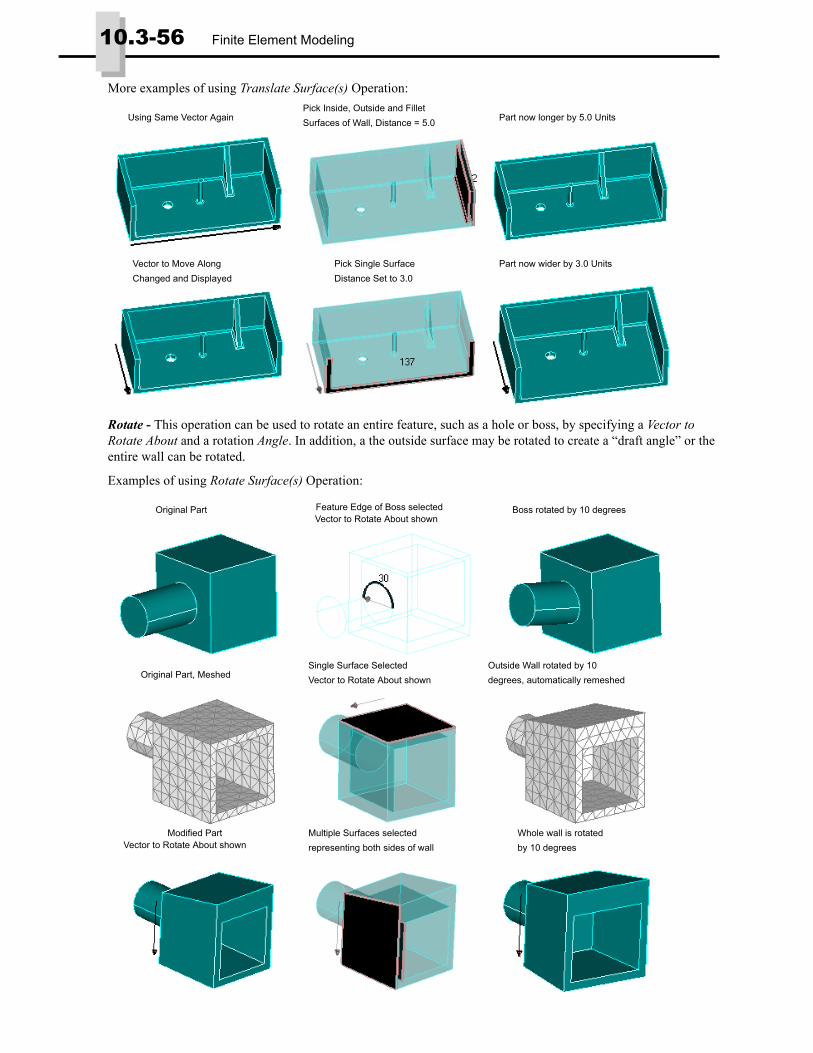
10.3-56 Finite Element Modeling
More examples of using Translate Surface(s) Operation:
Rotate - This operation can be used to rotate an entire feature, such as a hole or boss, by specifying a Vector to Rotate About and a rotation Angle. In addition, a the outside surface may be rotated to create a “draft angle” or the entire wall can be rotated.
Examples of using Rotate Surface(s) Operation:
Vector to Move Along Pick Single SurfaceDistance Set to 3.0
Part now wider by 3.0 Units
Using Same Vector AgainPick Inside, Outside and FilletSurfaces of Wall, Distance = 5.0 Part now longer by 5.0 Units
Changed and Displayed
Original PartVector to Rotate About shownFeature Edge of Boss selected Boss rotated by 10 degrees
Original Part, MeshedSingle Surface SelectedVector to Rotate About shown
Outside Wall rotated by 10degrees, automatically remeshed
Modified PartVector to Rotate About shown
Multiple Surfaces selectedrepresenting both sides of wall
Whole wall is rotatedby 10 degrees
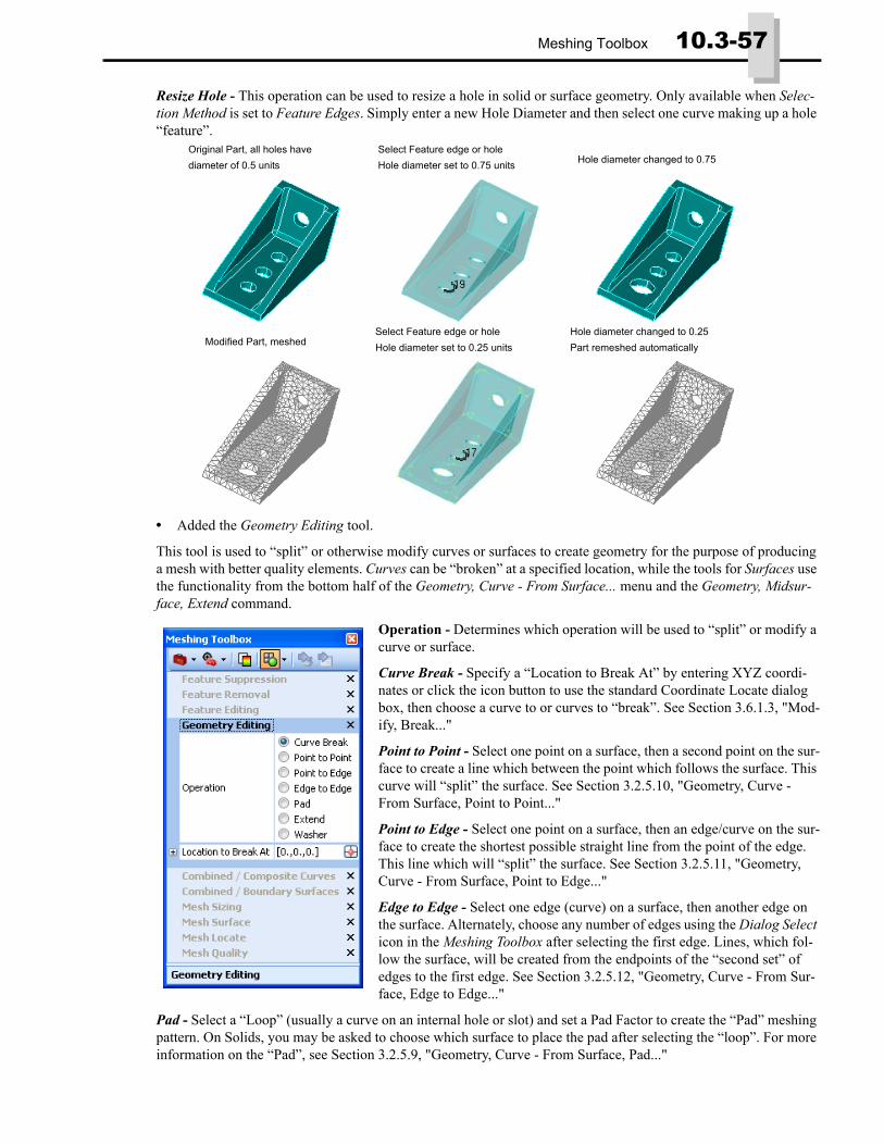
Meshing Toolbox 10.3-57
Resize Hole - This operation can be used to resize a hole in solid or surface geometry. Only available when Selec-tion Method is set to Feature Edges. Simply enter a new Hole Diameter and then select one curve making up a hole “feature”.
• Added the Geometry Editing tool.
This tool is used to “split” or otherwise modify curves or surfaces to create geometry for the purpose of producing a mesh with better quality elements. Curves can be “broken” at a specified location, while the tools for Surfaces use the functionality from the bottom half of the Geometry, Curve - From Surface... menu and the Geometry, Midsur-face, Extend command.
Operation - Determines which operation will be used to “split” or modify a curve or surface.
Curve Break - Specify a “Location to Break At” by entering XYZ coordi-nates or click the icon button to use the standard Coordinate Locate dialog box, then choose a curve to or curves to “break”. See Section 3.6.1.3, "Mod-ify, Break..."
Point to Point - Select one point on a surface, then a second point on the sur-face to create a line which between the point which follows the surface. This curve will “split” the surface. See Section 3.2.5.10, "Geometry, Curve - From Surface, Point to Point..."
Point to Edge - Select one point on a surface, then an edge/curve on the sur-face to create the shortest possible straight line from the point of the edge. This line which will “split” the surface. See Section 3.2.5.11, "Geometry, Curve - From Surface, Point to Edge..."
Edge to Edge - Select one edge (curve) on a surface, then another edge on the surface. Alternately, choose any number of edges using the Dialog Select icon in the Meshing Toolbox after selecting the first edge. Lines, which fol-low the surface, will be created from the endpoints of the “second set” of edges to the first edge. See Section 3.2.5.12, "Geometry, Curve - From Sur-face, Edge to Edge..."
Pad - Select a “Loop” (usually a curve on an internal hole or slot) and set a Pad Factor to create the “Pad” meshing pattern. On Solids, you may be asked to choose which surface to place the pad after selecting the “loop”. For more information on the “Pad”, see Section 3.2.5.9, "Geometry, Curve - From Surface, Pad..."
Original Part, all holes havediameter of 0.5 units
Select Feature edge or holeHole diameter set to 0.75 units Hole diameter changed to 0.75
Modified Part, meshedSelect Feature edge or holeHole diameter set to 0.25 units
Hole diameter changed to 0.25Part remeshed automatically

10.3-58 Finite Element Modeling
Extend - Mimics the Geometry, Midsurface, Extend command. Choose a single edge of a surface to extend with the Entity Select icon in the Meshing Toolbox or multiple edges using Dialog Select icon. See Section 3.3.4.5, "Extend..." for more information about the Extend Shape and Extend To options.
Washer - Select a circular curve and specify an Offset Distance. Works like Geometry, Curve - From Surface, Off-set Curve/Washer command when in Washer Mode. See Section 3.2.5.8, "Geometry, Curve - From Surface, Offset Curves/Washer..."
Some examples
• Added the Mesh Surface tool.
This tool may be used to mesh any number of surfaces in the model using options found in several different meshing com-mands (See Section 5.1.3.3, "Mesh, Geometry, Surface...", Section 5.1.2.15, "Mesh, Mesh Control, Approach On Sur-face", and Section 5.1.2.12, "Mesh, Mesh Control, Attributes On Surface" for more information).
When meshing surfaces which have already been meshed with this tool, the original mesh is always deleted, then the surfaces are remeshed.
Load Attributes from Surface - Allows you to choose a sur-face which has Mesh Attributes assigned, then loads those Mesh Attributes into the Mesh Surface tool. Now use the Select or Dialog Select icons in the Meshing Toolbox to mesh surfaces with these attributes. Enter a surface ID or click the “...” icon button to select a surface from the graphics window.
Property - Allows you to choose an existing property in the model to mesh/remesh surfaces. The default value is to “Use Meshing Attributes” which have been applied to the surface from previous meshing commands. A new property can also be created by clicking the “...” icon button, then the new property will automatically be set as the Property.
Note: If you select a surface which has no meshing attributes and/or property specified, the current specified attributes and/or property will be used.
Original Hole Pad (Factor = 1.0) Washer (Offset = 0.25)
Point to Edge Edge to Edge(s)Point to Point
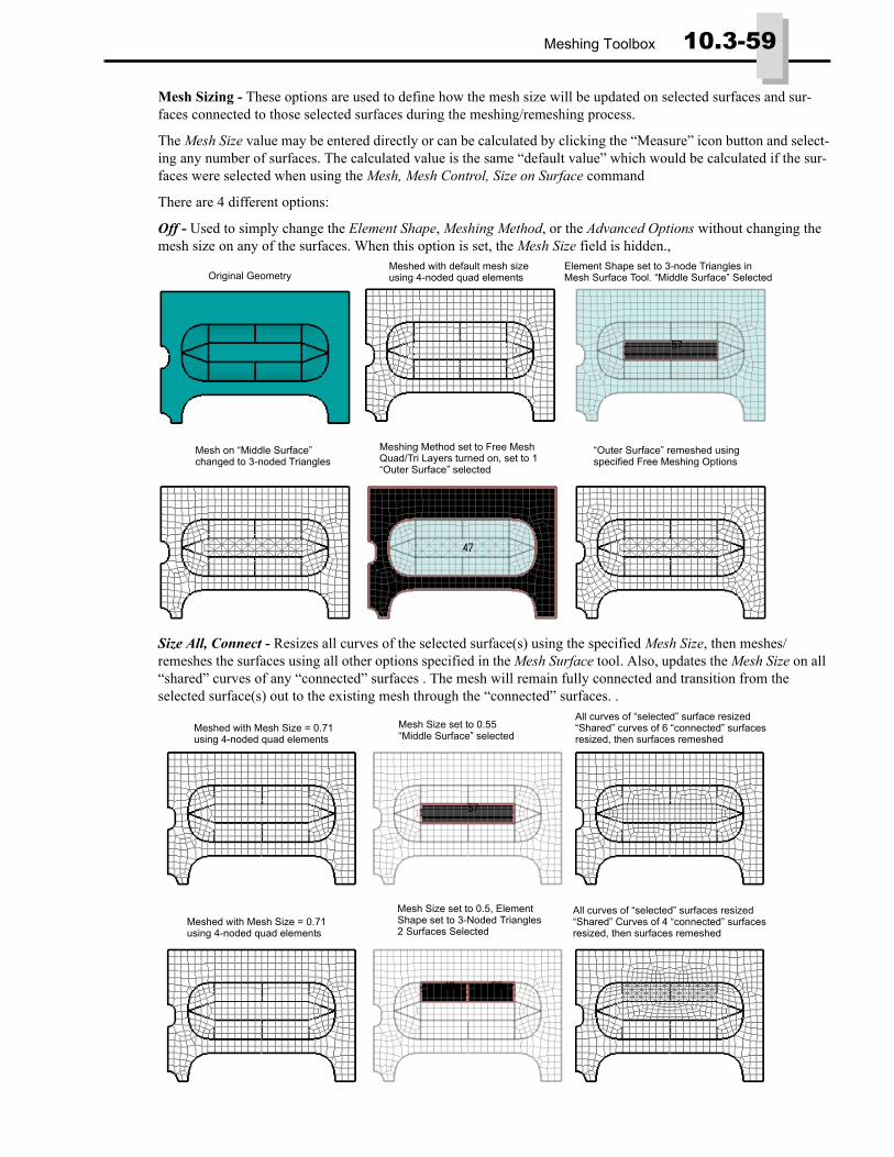
Meshing Toolbox 10.3-59
Mesh Sizing - These options are used to define how the mesh size will be updated on selected surfaces and sur-faces connected to those selected surfaces during the meshing/remeshing process.
The Mesh Size value may be entered directly or can be calculated by clicking the “Measure” icon button and select-ing any number of surfaces. The calculated value is the same “default value” which would be calculated if the sur-faces were selected when using the Mesh, Mesh Control, Size on Surface command
There are 4 different options:
Off - Used to simply change the Element Shape, Meshing Method, or the Advanced Options without changing the mesh size on any of the surfaces. When this option is set, the Mesh Size field is hidden.,
Size All, Connect - Resizes all curves of the selected surface(s) using the specified Mesh Size, then meshes/remeshes the surfaces using all other options specified in the Mesh Surface tool. Also, updates the Mesh Size on all “shared” curves of any “connected” surfaces . The mesh will remain fully connected and transition from the selected surface(s) out to the existing mesh through the “connected” surfaces. .
Original GeometryMeshed with default mesh size Element Shape set to 3-node Triangles inusing 4-noded quad elements Mesh Surface Tool. “Middle Surface” Selected
Mesh on “Middle Surface” changed to 3-noded Triangles
Meshing Method set to Free MeshQuad/Tri Layers turned on, set to 1“Outer Surface” selected
“Outer Surface” remeshed usingspecified Free Meshing Options
Meshed with Mesh Size = 0.71using 4-noded quad elements
Mesh Size set to 0.55“Middle Surface” selected
All curves of “selected” surface resized“Shared” curves of 6 “connected” surfacesresized, then surfaces remeshed
Meshed with Mesh Size = 0.71using 4-noded quad elements
Mesh Size set to 0.5, Element All curves of “selected” surfaces resized“Shared” Curves of 4 “connected” surfacesresized, then surfaces remeshed
Shape set to 3-Noded Triangles2 Surfaces Selected

10.3-60 Finite Element Modeling
Size All, Disconnect - Resizes all curves of the selected surface(s) using the specified Mesh Size, then meshes/remeshes the surfaces using all other options specified in the Mesh Surface tool. No effort is made to keep the mesh on any surrounding surfaces in the model “connected” to the mesh on the selected surface(s).
Size, Internal/Free Edges - Only resizes “internal curves” or “free edges” of selected surface(s) using the specified Mesh Size and other options set in the Mesh Surface tool. All curves “shared” by selected surface(s) and non-selected surfaces will NOT be resized.
Element Shape - Choose to mesh the surface with one of 4 options, represented by pictures. From left, the pictures represent 3-noded linear triangles, 6-noded parabolic triangles, 4-noded linear quads, and 8-noded parabolic quads.
Meshing Method - Choose between Free Mesh and Mapped Mesh. Depending on what method is selected, differ-ent options will be available.
Free Mesh - The Free Meshing Options include Quad/Tri Layers and Min Elements Between Boundaries which are also found in the Mesh, Geometry, Surface command (see Section 5.1.3.3, "Mesh, Geometry, Surface..."), Surface Growth Factor and Refinement Ratio which are also found in the Mesh, Mesh Control, Size on Surface command (see Section 5.1.2.4, "Mesh, Mesh Control, Size On Surface..."), and the Approach Options drop-down, which allows you to choose any of the 4 “free meshing” approach options found in Mesh, Mesh Control, Approach on Surface command (see Section 5.1.2.15, "Mesh, Mesh Control, Approach On Surface")
Mapped Mesh - The Mapped Meshing Options include Min Elements Between Boundaries which is also found in the Mesh, Geometry, Surface command (see Section 5.1.3.3, "Mesh, Geometry, Surface..."), and Auto Mapped Approach, which is on by default. When Auto Mapped Approach is “on”, the tool will examine the selected surface and determine if it is a good candidate for one of the “mapped meshing” approaches available in the Mesh, Mesh Control, Approach on Surface command. If so, the approach will be set automatically and the curves of the surface resized, if allowed by the current Mesh Sizing option in the Mesh Surface tool. If not, the best possible “mapped
Meshed with Mesh Size = 0.5using 4-noded quad elements
Mesh Size set to 0.9, Element All curves of “selected” surfacesShape set to 3-Noded Triangles“Middle” Surface Selected
resized, then automatically remeshedwith 3-noded triangles
Meshed with Mesh Size = 0.71using 4-noded quad elements
Mesh Size set to 0.411 Surfaces selected
All internal curves of “selected” surfaces
Meshed with Mesh Size = 0.71using 4-noded quad elements
Mesh Size set to 0.4, Element Only single curve “shared” between the 2Shape set to 3-Noded Triangles2 Surfaces Selected
resized, then selected surfaces remeshed,while non-selected surfaces unchanged.
selected surfaces has sizing updated, then2 selected surfaces remeshed with triangles
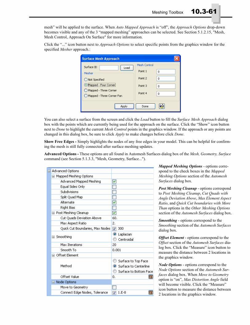
Meshing Toolbox 10.3-61
mesh” will be applied to the surface. When Auto Mapped Approach is “off”, the Approach Options drop-down becomes visible and any of the 3 “mapped meshing” approaches can be selected. See Section 5.1.2.15, "Mesh, Mesh Control, Approach On Surface" for more information.
Click the “...” icon button next to Approach Options to select specific points from the graphics window for the specified Mesher approach.:
You can also select a surface from the screen and click the Load button to fill the Surface Mesh Approach dialog box with the points which are currently being used for the approach on the surface. Click the “Show” icon button next to Done to highlight the current Mesh Control points in the graphics window. If the approach or any points are changed in this dialog box, be sure to click Apply to make changes before click Done.
Show Free Edges - Simply highlights the nodes of any free edges in your model. This can be helpful for confirm-ing the mesh is still fully connected after surface meshing updates.
Advanced Options - These options are all found in Automesh Surfaces dialog box of the Mesh, Geometry, Surface command (see Section 5.1.3.3, "Mesh, Geometry, Surface...").
Mapped Meshing Options - options corre-spond to the check boxes in the Mapped Meshing Options section of the Automesh Surfaces dialog box.
Post Meshing Cleanup - options correspond to Post Meshing Cleanup, Cut Quads with Angle Deviation Above, Max Element Aspect Ratio, and Quick Cut boundaries with More Than options in the Other Meshing Options section of the Automesh Surfaces dialog box.
Smoothing - options correspond to the Smoothing section of the Automesh Surfaces dialog box.
Offset Element - options correspond to the Offset section of the Automesh Surfaces dia-log box. Click the “Measure” icon button to measure the distance between 2 locations in the graphics window.
Node Options - options correspond to the Node Options section of the Automesh Sur-faces dialog box. When Move to Geometry option is “on”, Max Distortion Angle field will become visible. Click the “Measure” icon button to measure the distance between 2 locations in the graphics window.

10.3-62 Finite Element Modeling
PostProcessing Toolbox• PostProcessing dockable pane is completely new for 10.2.
The PostProcessing Toolbox provides a single, consolidated location in the interface from which to postprocess results from an analysis. First, choose a “Style” from either the Deform or Contour tool, then use the unique set of options for that “Style” to create or change what is displayed in the graphics window. The toolbox itself allows changes to be made “on-the-fly” or when directed by the user.
The PostProcessing Toolbox brings together options for each style which are found in several different View... com-mands. Additional information on most of these options may be found in Section 8.2, "Types of Views - View Select...", Section 8.3, "View Options - PostProcessing" and Section 8.4, "Specialized Post-processing".
PostProcessing Toolbox IconsToggle Tools menu - By default, both “tools” will be visible in the PostProcessing Toolbox.
Using the drop-down menu from this icon, make all of the tools visible or hidden at once using “Toggle All Tools” or individually toggle them on and off by choosing the individual “tool name” (for example, Deform) from the menu. When a tool is visible, there will be a check mark next to it in the list.
Here is a short description of each tool:
Deform - Sets the “Deformed Style”. Choose from Undeformed, Deformed, Animate, Animate - Multi-Set, Vector, Trace, or Streamline. Once a “Style” has been chosen, select Results. Also, unique Options become available for each “Style”.
Contour - Sets the “Contour Style”. Choose from No Contours, Contour, Criteria, Beam Diagram, IsoSurface, Section Cut, or Vector. Once a “Style” has been chosen, select Results. Also, unique Options become available for each “Style”.
Reload - Reloads the PostProcessing Toolbox with the current postprocessing options set in the model.
Undeformed/No Contours - Simply sets the Deform Style to Undeformed and Contour Style to No Contours.
Deformed Style - Choose a Deform Style from the drop-down menu.
Contour Style - Choose a Contour Style from the drop-down menu.
Auto Redraw - When On, which is the default, changes made to Style, Results, or Options will be plotted to the graphics window “on-the-fly”. When Off, click the Manual Redraw button or use the Window, Redraw (Crtl+D) or Window, Regenerate (Ctrl+G) command to update the image in the graphics window.
Manual Redraw - Click this button to “Redraw” the graphics window.
Deform toolChoose a Style in the Deform tool. Choices are Undeformed, Deformed, Animate, Animate - MultiSet, Vector, Trace, and Streamline. For each Style, a unique set of options becomes available.
ResultsSelect the Output Set and Output Vector to display for each Deform Style. With Style set to Animate - MultiSet or Trace, the Final Output Set should also be specified, with the option to include an Increment value to use every “nth” out-put set in the animation.
The Output Set, Final Output Set, and Output Vector options have some additional controls which make it easier to move from one output set or output vector to another.
Toggle ToolsRoload
Undeformed/No Contour
Deformed Style
Contour Style
Auto Redraw
Manual Redraw
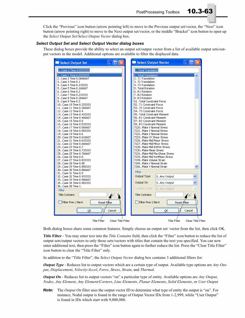
PostProcessing Toolbox 10.3-63
Click the “Previous” icon button (arrow pointing left) to move to the Previous output set/vector, the “Next” icon button (arrow pointing right) to move to the Next output set/vector, or the middle “Bracket” icon button to open up the Select Output Set/Select Output Vector dialog box.
Select Output Set and Select Output Vector dialog boxesThese dialog boxes provide the ability to select an output set/output vector from a list of available output sets/out-put vectors in the model. Additional options are available to filter the displayed data.
Both dialog boxes share some common features. Simply choose an output set/ vector from the list, then click OK.
Title Filter - You may enter text into the Title Contains field, then click the “Filter” icon button to reduce the list of output sets/output vectors to only those sets/vectors with titles that contain the text you specified. You can now enter additional text, then press the “Filter” icon button again to further reduce the list. Press the “Clear Title Filter” icon button to clear the “Title Filter” only.
In addition to the “Title Filter”, the Select Output Vector dialog box contains 3 additional filters for:
Output Type - Reduces list to output vectors which are a certain type of output. Available type options are Any Out-put, Displacement, Velocity/Accel, Force, Stress, Strain, and Thermal.
Output On - Reduces list to output vectors “on” a particular type of entity. Available options are Any Output, Nodes, Any Element, Any Element/Corners, Line Elements, Planar Elements, Solid Elements, or User Output
Note: The Output On filter uses the output vector ID to determine what type of entity the output is “on”. For instance, Nodal output is found in the range of Output Vector IDs from 1-2,999, while “User Output” is found in IDs which start with 9,000,000.
Title Filter Clear Title Filter Clear Title FilterTitle Filter

10.3-64 Finite Element Modeling
Complex Type - Only available when “complex data” exists in the selected output set. Reduces list to output vec-tors of a particular “complex type”. Available options are Any Output, Magnitude, Phase, Real Component, and Imaginary Component.
Filter Next/Prev - When the Filter Prev/Next option is on, the Previous and Next controls in the PostProcessing toolbox will only move between the “filtered” output sets/output vectors.
Reset Filter - Click Reset Filter button to clear ALL filters and turn off the Filter Prev/Next option.
Options - Deform toolMany of the options are shared between several different Deform Styles, while others are only used for one particu-lar style. Please see the table below to see which options are available in a particular Style. Descriptions of all the options follows the table. “Top Level” options appear in Bold Text in the table.
Transform - Allows “transformation” of the Deformation Output Vector. Vector may be transformed using the Nodal Output Coordinate System of each node or into any Coordinate System in the model. See Displacement Out-put Vector Transformation in Section 8.2.2.2, "Selecting Data for a Deformed or Contour Style" for more info.
Active Components - Choose to include X, Y, and/or Z components when transforming the Deformation Output Vector. When “checked”, component is included.
Scale - Sets the Scale for the Deformation Output Vector. Default is % of Model, which uses the Max % Model value to determine how the deformation values will be scaled in the graphics window. Other option is Actual Deformations, which uses the actual deformations at each node combined with the Scale Actual By factor.
Max % Model - Used when Scale is set to % of Model. Value represents a percentage of overall model size. Largest deformation in the model will be scaled by this value, then all other deformations are linearly interpolated between 0 and specified value.
Scale Actual By - Used when Scale is set to Actual Deformations. Actual deformation values are multiplied by this Scale Factor and then displayed graphically.
Scale Based on Group - Off by default. When On, the largest deformation value from displayed group(s) is used to graphically display the deformed model.
Deform Options Deformed Animate Animate MultiSet Vector Trace Streamline
Transform * * * * * *Active Components (X;Y;Z) * * * * * *Scale * * * * *Max % Model/Scale Actual By * * * * *Scale Based on Group * * * * *Deform Relative To * * * * *Node ID * * * * *Deformed Model * * * * *Animate Deformation * * *Use View Color * * * * *Default Direction * * * * *Undeformed Model * * * *Use View Color * * * *Animation * *Shape *Frames *Delay * *Animation Control * *Vector options *Trace options *Locations options *Streamline options *

PostProcessing Toolbox 10.3-65
Deformed Relative To - Model is deformed relative to the Origin (0,0,0 in the model) by default. Other option is to deform the model relative to a Fixed Node anywhere in the model.
Node ID - Specifies the Node ID to be used when Deform Relative To is set to Fixed Node. Click the icon button to the left to graphically select a Node ID from the screen.
Deformed Model - Specify options for the display of the Deformed Model.
Animate Deformation - On by default. When Off, the model will animate the selected contour style, but the model will not be deformed. This is helpful in heat transfer and transient models.
Use View Color - Off by default. When On, deformed model will be shown using the specified View Color (Not used on elements which have Contour Style applied). Click the “Color Wheel” icon button to select a View Color from the Color Palette dialog box.
Default Direction - Only used when specified Deformation Output Vector contains scalar values instead of vectors. Model will deform in the chosen direction based on the scalar values.
Undeformed Model - Off by default. When On, an image of the Undeformed model will be displayed along with the deformed model
Use View Color - On by default. Sets the View Color for the Undeformed Model. Click the “Color Wheel” icon but-ton to select a View Color from the Color Palette dialog box. When Off, the Undeformed Model will use entity col-ors.
Animation - Specify options for Animations of specific Deform Styles.
Shape - Choose between a Linear Interpolation and a Sinusoidal distribution of the frames in the animation. Also, choose Full or Full Absolute to see the model Load and Unload. Choose Half or Half Absolute to only animate the model in the loaded direction. See Section 8.3.4, "Animated Style" for more information.
Frames - Specify number of frames for animation. Default value is 4.
Delay - Specify the delay between each frame. Default value is 101. Larger values result in slower animations.
Animation Control - Click button to open the Animation Control dialog box. Speed and shape of animation can be controlled. Also, animation may be paused and then moved frame by frame.
Vector - Specify options for display of the Vector Deform Style.
Label - Choose a Label Mode for Vector Display. Default is No Labels. Other options are Output Values (Labels on all Deformed Vectors) and Top Percent (Labels only on Deformed Vectors which fall into specified top percentile). When Top Percent is chosen for Label, the Top Percent field will become visible. Default is 10, which means only the vectors with the top 10% of Deformed Values will be labeled.
Color - Sets the color of the Vectors for the Vector Deform Style. Click the “Color Wheel” icon button to select a color for the Vector plot from the Color Palette dialog box.
Arrowheads - On by default. When On, displays arrowheads at the 'tip' of the vectors. When Off, no arrowheads will be displayed.
Component Vectors - Off by default. When On, displays the Deformation Vectors as XYZ Component vectors instead of a single resultant vector.
Show As Solid - Off by default. When On, Vectors are displayed as solid vectors instead of lines.
Trace - Specify options for Trace Deform Style. Trace creates trace plots on the screen for a single node, a group of nodes, or every node in the model.
At Locations - Choose Trace locations. Full Model is the default. Other options are Single Node (must specify node below in Node ID) or choose a group which already exists in the model (group must contain nodes to see any trace plots).

10.3-66 Finite Element Modeling
Length - Choose to see the entire length of the trace plot(s) from the beginning (Full Length) or have them animate as the model deforms (Animate Growth). Default is Full Length.
Label - Label the Trace Locations, only when Show Locations option is On. Default is No Labels. Other options are to label each trace location for each node using the Set ID of each Output Set used to create the plot or the Set Value.
Color - Sets the color of the Trace plot. Click the “Color Wheel” icon button to select a color for the Trace plot from the Color Palette dialog box.
Show Locations - Places a marker along the Trace line representing the trace location at each Output Set being used to create the Trace plot.
Locations - Choose locations for Streamlines in Streamline Deform Style. Default is Specified Location (click but-ton next to Location to choose graphically). At Point option will use any existing Point in the model. Other option is to choose a Group in the model (Group must contains points to create Streamlines).
Location - Used by Specified Location option. Click button to select a “location” for a single Streamline from the graphics window or enter coordinates manually in the X, Y, and/or Z fields.
Select Point for Streamline Location - Used by At Point option. Enter a Point ID or click icon button to select a point graphically.
Dynamic Location - Click button to display the Dynamic Streamline Control dialog box. Dynamically move, extend, or shorten a Streamline plot. Set the Radio button on the left side to modify the X, Y, or Z position of the Streamline.
Streamline - Specify options for display of the Streamline Deform Style.
Draw Start - Off by default. When On, the start location of the Streamline(s) will be drawn in the graphics window.
Use View Color - Off by default. When On, the Streamline(s) will be drawn using the View Color instead of Con-tour Colors. Click the “Color Wheel” icon button to select a View Color from the Color Palette dialog box.
Parameters (Streamline) - These values may be used to alter the appearance of the Streamline(s) in the model.
Runge-Kutta Order - Streamlines are evaluated using the Runge-Kutta Numerical method. Value indicates the order being used by the method. Values range from 1 to 4, with 2 being the default. Increasing the order generally increases accuracy, but also increases calculation time.
Tolerance - Value is used to determine when a Streamline is entering or leaving an element. Tolerance has no units and is based on each element's size. Default value is 1.0E-5. Lowering the Tolerance value generally increases accuracy, but also increases calculation time.
Max Length Factor (x Model) - Value is multiplied by the model bounding box diagonal to accommodate stream-lines which are longer than model bounding box diagonal, which is somewhat common. Error will occur if this value is not large enough to accommodate very lengthy streamlines.
Minimum Speed (% of Max) - Value represents a percentage of Maximum Velocity in the selected output vector. Lowering this value will allow display of streamlines with lower velocities relative to the Maximum Velocity.
Contour toolChoose a Style in the Contour tool. Choices are No Contours, Contour, Criteria, Beam Diagram, IsoSuface, Section Cut, and Contour Vector. For each Style, a unique set of options becomes available.
ResultsSelect the Output Set and Output Vector to display for each Contour Style. An optional Additional Vector can be specified when Style is set to Contour, while a separate control exists for choosing Contour Vectors when Style is set to Contour Vector . See Section , "Deform tool" for more information on the unique controls in the Results sec-tion, as well as the Select Output Set and Select Output Vector dialog boxes.
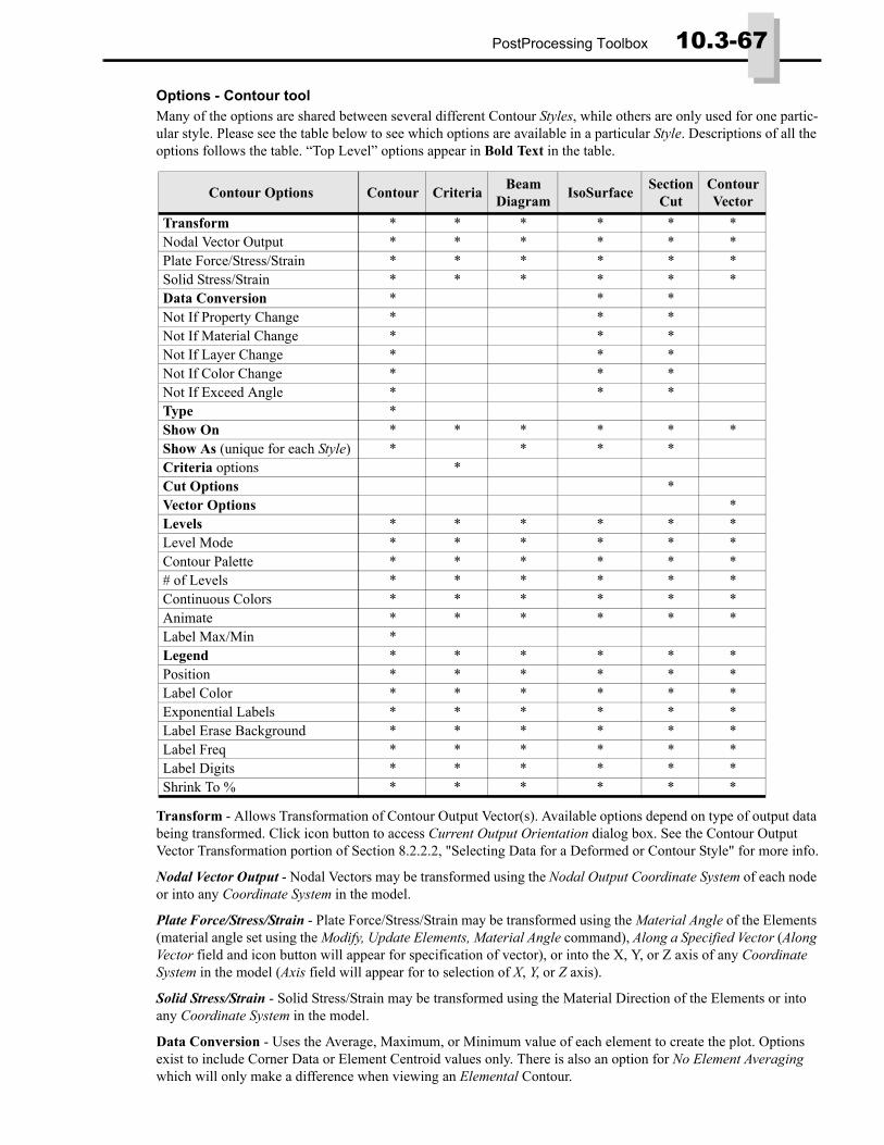
PostProcessing Toolbox 10.3-67
Options - Contour toolMany of the options are shared between several different Contour Styles, while others are only used for one partic-ular style. Please see the table below to see which options are available in a particular Style. Descriptions of all the options follows the table. “Top Level” options appear in Bold Text in the table.
Transform - Allows Transformation of Contour Output Vector(s). Available options depend on type of output data being transformed. Click icon button to access Current Output Orientation dialog box. See the Contour Output Vector Transformation portion of Section 8.2.2.2, "Selecting Data for a Deformed or Contour Style" for more info.
Nodal Vector Output - Nodal Vectors may be transformed using the Nodal Output Coordinate System of each node or into any Coordinate System in the model.
Plate Force/Stress/Strain - Plate Force/Stress/Strain may be transformed using the Material Angle of the Elements (material angle set using the Modify, Update Elements, Material Angle command), Along a Specified Vector (Along Vector field and icon button will appear for specification of vector), or into the X, Y, or Z axis of any Coordinate System in the model (Axis field will appear for to selection of X, Y, or Z axis).
Solid Stress/Strain - Solid Stress/Strain may be transformed using the Material Direction of the Elements or into any Coordinate System in the model.
Data Conversion - Uses the Average, Maximum, or Minimum value of each element to create the plot. Options exist to include Corner Data or Element Centroid values only. There is also an option for No Element Averaging which will only make a difference when viewing an Elemental Contour.
Contour Options Contour Criteria Beam Diagram IsoSurface Section
CutContour Vector
Transform * * * * * *Nodal Vector Output * * * * * *Plate Force/Stress/Strain * * * * * *Solid Stress/Strain * * * * * *Data Conversion * * *Not If Property Change * * *Not If Material Change * * *Not If Layer Change * * *Not If Color Change * * *Not If Exceed Angle * * *Type *Show On * * * * * *Show As (unique for each Style) * * * *Criteria options *Cut Options *Vector Options *Levels * * * * * *Level Mode * * * * * *Contour Palette * * * * * *# of Levels * * * * * *Continuous Colors * * * * * *Animate * * * * * *Label Max/Min *Legend * * * * * *Position * * * * * *Label Color * * * * * *Exponential Labels * * * * * *Label Erase Background * * * * * *Label Freq * * * * * *Label Digits * * * * * *Shrink To % * * * * * *

10.3-68 Finite Element Modeling
Not If Property Change - Elemental Contours Only - On by default, will NOT average between elements of differ-ent properties. When off, averaging occurs between elements of different properties.
Not If Material Change - Elemental Contours Only - Only available when 'Not If Property Change' is off. On by default. When Off, averaging occurs between elements of different materials
Not If Layer Change - Elemental Contours Only - Off by default, will average between elements on different Lay-ers. When On, averaging does NOT occur between elements on different Layers.
Not If Color Change - Elemental Contours Only - Off by default, will average between elements on different Col-ors. When On, averaging does NOT occur between elements on different Colors.
Not If Exceed Angle - Elemental Contours Only - On by default, will NOT average between elements which have a Break Angle of more than the specified angle value (Default Value is 20 degrees). When Off, averaging occurs regardless of angle between elements.
Type - Choose Type of Contour to display. Choose between Nodal, Elemental, or Match Output. When Match Out-put is used, FEMAP will display a Nodal Contour when plotting nodal output or an Elemental Contour for elemen-tal output.
Double-Sided Planar - Elemental Contours Only - Off by default. When On, the 'other side' of a plate contour will be displayed along with selected output vector (For Example, if Plate Top X normal Stress is selected, then Plate Bot X Normal Stress will be displayed on the other side of the plate elements).
Show On - Select to create a plot on a group while the rest of the model is visible. Choose the Active Group or Select any group in the model from the drop-down list. Group should include elements.
Show As - The Show As option(s) differ for each Style which has it available. Each is described below.
Contour - Choose between showing a Filled contour and a Line Contour. Filled is the default.
Beam Diagram - The “top-level” Show As option allows you to display a Beam Diagram plot as a Beam Diagram or a Beam Contour.
Additional Show As options for Beam Diagram plots include:
Label - By default, set to No Labels. Other options are Labels at Nodes (Output values displayed at nodes of beam elements) and Labels at Peaks (Output values displayed at peaks of Beam Diagrams).
Direction - Select a direction for ALL beam diagrams to be displayed. Choose from Element Y, Element Z, Global X, Global Y, or Global Z. These 5 options are also available with the End B values reversed, which is needed to properly display Beam Diagrams using output from certain FE solvers.
Show Reversed - Off by default. When on, reverses the direction which the Beam Diagrams will be displayed.
Scale % - Used to set the overall height of the Beam Diagrams. By default, largest value is shown at 10% of model size. Different value may be entered directly or slider may be used to increase Scale %.
Border Color - Sets the color of the border of each Beam Diagram. Click the Color Wheel button to select a color from the Color Palette dialog box.
IsoSurface - The “top-level” Show As option allows you to choose how the IsoSurface will be displayed. IsoSur-face is the default. Other options are IsoLine (Line representation instead of Surface) and Contour on Deform IsoS-urface (displays Output Values at areas in the model with the same deformation value, which must be entered in the At Value field).
Additional Show As options for IsoSurface plots include:
Number - By default, a Single IsoSurface/IsoLine will be shown. When set to Single, a value should be entered in the At Value field. Other option, Use Contour Levels will create an IsoSurface/IsoLine for each Contour Level in the model (i.e., # of Levels set to 16 creates 16 IsoSurfaces/IsoLines on the model).
Contour Mode - IsoLines Only. Default is to show Isolines Only. Other Options are Contour Above (Only contours values above specified value) and Contour Below (only contours values below specified value).
IsoLine Width - IsoLines Only. Sets the width of the IsoLines. Default is 1. Value may be entered directly or chosen using the slider to increase IsoLine thickness.
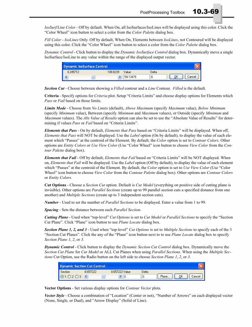
PostProcessing Toolbox 10.3-69
IsoSurf/Line Color - Off by default. When On, all IsoSurfaces/IsoLines will be displayed using this color. Click the “Color Wheel” icon button to select a color from the Color Palette dialog box.
Fill Color - IsoLines Only. Off by default, When On, Elements between IsoLines, not Contoured will be displayed using this color. Click the “Color Wheel” icon button to select a color from the Color Palette dialog box.
Dynamic Control - Click button to display the Dynamic IsoSurface Control dialog box. Dynamically move a single IsoSurface/IsoLine to any value within the range of the displayed output vector.
Section Cut - Choose between showing a Filled contour and a Line Contour. Filled is the default.
Criteria - Specify options for Criteria plot. Setup “Criteria Limits” and choose display options for Elements which Pass or Fail based on those limits.
Limits Mode - Choose from No Limits (default), Above Maximum (specify Maximum value), Below Minimum (specify Minimum value), Between (specify Minimum and Maximum values), or Outside (specify Minimum and Maximum values). The Abs Value of Results option can also be set to use the “Absolute Value of Results” for deter-mining if values Pass or Fail based on “Criteria Limits”.
Elements that Pass - On by default, Elements that Pass based on “Criteria Limits” will be displayed. When off, Elements that Pass will NOT be displayed. Use the Label option (On by default), to display the value of each ele-ment which “Passes” at the centroid of the Element. By default, the Color option is set to Contour Colors. Other options are Entity Colors or Use View Color (Use “Color Wheel” icon button to choose View Color from the Con-tour Palette dialog box).
Elements that Fail - Off by default, Elements that Fail based on “Criteria Limits” will be NOT displayed. When on, Elements that Fail will be displayed. Use the Label option (Off by default), to display the value of each element which “Passes” at the centroid of the Element. By default, the Color option is set to Use View Color (Use “Color Wheel” icon button to choose View Color from the Contour Palette dialog box). Other options are Contour Colors or Entity Colors.
Cut Options - Choose a Section Cut option. Default is Cut Model (everything on positive side of cutting plane is invisible). Other options are Parallel Sections (create up to 99 parallel section cuts a specified distance from one another) and Multiple Sections (create up to 3 independent section cuts).
Number - Used to set the number of Parallel Sections to be displayed. Enter a value from 1 to 99.
Spacing - Sets the distance between each Parallel Section.
Cutting Plane - Used when “top-level” Cut Options is set to Cut Model or Parallel Sections to specify the “Section Cut Plane”. Click “Plane” icon button to use Plane Locate dialog box.
Section Plane 1, 2, and 3 - Used when “top-level” Cut Options is set to Multiple Sections to specify each of the 3 “Section Cut Planes”. Click the any of the “Plane” icon button next to to use Plane Locate dialog box to specify Section Plane 1, 2, or 3.
Dynamic Control - Click button to display the Dynamic Section Cut Control dialog box. Dynamically move the Section Cut Plane for Cut Model or ALL Cut Planes when using Parallel Sections. When using the Multiple Sec-tions Cut Option, use the Radio button on the left side to choose Section Plane 1, 2, or 3.
Vector Options - Set various display options for Contour Vector plots.
Vector Style - Choose a combination of “Location” (Center or not), “Number of Arrows” on each displayed vector (None, Single, or Dual), and “Arrow Display” (Solid of Line).

10.3-70 Finite Element Modeling
Length - Options for setting the length of Contour Vectors. Adjust Length to Value is On by default. Arrow lengths are adjusted so longer arrows represent larger values. When Off, all arrows are the same length. Arrow Length value may be set from 0.01 to 1000 to specify the length of the longest vector arrow (Adjust Length to Value = On) or all arrows (Adjust Length to Value = Off).
Label - Off by default. When On, displays label of Contour Vector value. Exponential Labels are Off by default. When On, Label values are displayed using Exponents (Scientific Notation). Use Label Digits value to vary the number of significant digits.
Levels - Set various options for Contour/Criteria Levels, which are used in all Contour Styles.
Level Mode - Options for how the “Max and Min” values for Contour/Criteria Levels are determined. Automatic is the default. Auto-Group will automatically use the “Max and Min” values of the displayed groups. Max Min requires values be entered for Maximum Level and Minimum Level. User Defined uses Maximum Level and Mini-mum Level along with Specify Levels to fully customize the Contour/Criteria Levels.
Contour Palette - Choose between using the Standard Palette, which is the default, or a User Palette. When set to Standard Palette, click the “Color Range” icon button to open the Contour/Criteria Levels dialog box. See Section 8.3.10.3, "Level Modes". When set to User Palette, click the “Color Range” icon button to open the User Defined Contour Color Palette dialog box. See Section 8.3.10.4, "User-Defined Contour Palette".
# of Levels - Specifies the number of Contour/Criteria Levels to use when Contour Palette is set to Standard Pal-ette.
Continuous Colors - On by default. When On, contours are blended from one color to the next creating a “contin-uous” contour. When Off, one color level stops, then another begins to create a “fringe” contour plot.
Animate - On by default. When On, the contour values will animate as the model animates. This animation is sim-ply a linear interpolation of the values from start to finish of the animation. When Off, Contour colors remain con-stant as the model animates.
Label Max/Min - Off by default. When On, the “Maximum and Minimum” values of the displayed contour will be labeled. The labels are located where these values occur in the model.
Legend - On by default. When On, the Contour/Criteria Legend will be displayed. When Off, no Legend will be visible.
Position - Choose the position of the Legend. Default is Center Right. Other options are Top Left, Top Center, Top Right, Center Left, Bottom Left, Bottom Center, and Bottom Right. All Legends are vertical except Top Center and Bottom Center.
Label Color - Sets the Label Color of the Legend. Default is to use Contour Colors. Other option is Use View Color, which can then be set using the View Color option directly below.
Exponential Labels - Off by default. When On, Legend values are displayed using Exponents (Scientific Nota-tion). Use Label Digits value to vary the number of significant digits in the Legend.
Label Erase Background - Off by default. When On, the background will be erased around labels in order to make them easier to read. Does all labels, not just Labels in the Legend.
Label Freq- Specifies the frequency of the Contour/Criteria Levels are labeled in the Legend. When set to 0 or 1, all Levels are labeled. When set to 2, every other level is labeled, set to 3, every 3rd level, etc.
Label Digits - Used to set the number of significant digits displayed in the Legend.
Shrink to % - May be used to shrink the Legend to a % of original size. % Values may be entered directly or by using the Slider. When Position is using any of the options which mention 'Center', the Legend is shrunk on both ends towards the middle. All other Position options are shrunk in one direction only.
Entity Editor• Added “Explicit Time Step” field to Element Quality section when an element is loaded in the Editor.
API Programming• Updated to new version API Programing tool, which now shows line numbers (which can be turned off) and
changes some of the look and feel for more efficient use.
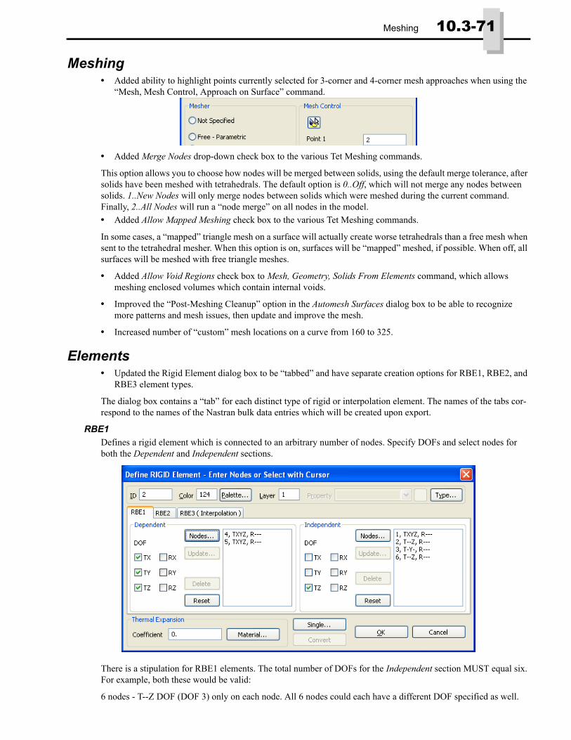
Meshing 10.3-71
Meshing• Added ability to highlight points currently selected for 3-corner and 4-corner mesh approaches when using the
“Mesh, Mesh Control, Approach on Surface” command.
• Added Merge Nodes drop-down check box to the various Tet Meshing commands.
This option allows you to choose how nodes will be merged between solids, using the default merge tolerance, after solids have been meshed with tetrahedrals. The default option is 0..Off, which will not merge any nodes between solids. 1..New Nodes will only merge nodes between solids which were meshed during the current command. Finally, 2..All Nodes will run a “node merge” on all nodes in the model.• Added Allow Mapped Meshing check box to the various Tet Meshing commands.
In some cases, a “mapped” triangle mesh on a surface will actually create worse tetrahedrals than a free mesh when sent to the tetrahedral mesher. When this option is on, surfaces will be “mapped” meshed, if possible. When off, all surfaces will be meshed with free triangle meshes.
• Added Allow Void Regions check box to Mesh, Geometry, Solids From Elements command, which allows meshing enclosed volumes which contain internal voids.
• Improved the “Post-Meshing Cleanup” option in the Automesh Surfaces dialog box to be able to recognize more patterns and mesh issues, then update and improve the mesh.
• Increased number of “custom” mesh locations on a curve from 160 to 325.
Elements• Updated the Rigid Element dialog box to be “tabbed” and have separate creation options for RBE1, RBE2, and
RBE3 element types.
The dialog box contains a “tab” for each distinct type of rigid or interpolation element. The names of the tabs cor-respond to the names of the Nastran bulk data entries which will be created upon export.
RBE1Defines a rigid element which is connected to an arbitrary number of nodes. Specify DOFs and select nodes for both the Dependent and Independent sections.
There is a stipulation for RBE1 elements. The total number of DOFs for the Independent section MUST equal six. For example, both these would be valid:
6 nodes - T--Z DOF (DOF 3) only on each node. All 6 nodes could each have a different DOF specified as well.
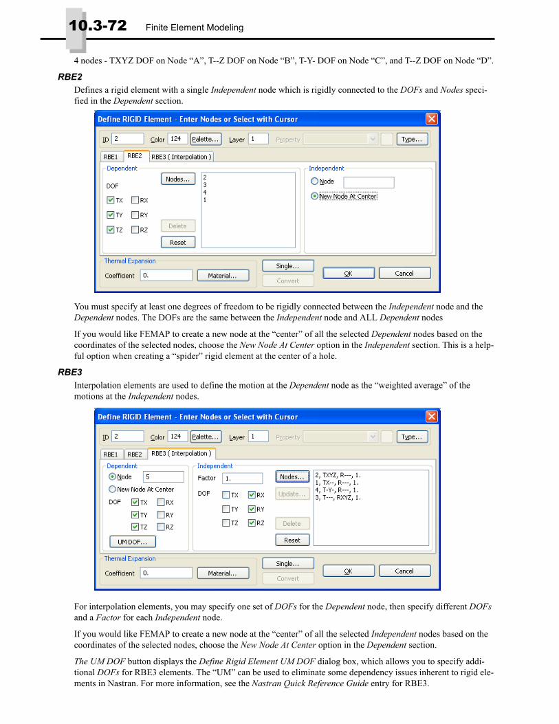
10.3-72 Finite Element Modeling
4 nodes - TXYZ DOF on Node “A”, T--Z DOF on Node “B”, T-Y- DOF on Node “C”, and T--Z DOF on Node “D”.
RBE2Defines a rigid element with a single Independent node which is rigidly connected to the DOFs and Nodes speci-fied in the Dependent section.
You must specify at least one degrees of freedom to be rigidly connected between the Independent node and the Dependent nodes. The DOFs are the same between the Independent node and ALL Dependent nodes
If you would like FEMAP to create a new node at the “center” of all the selected Dependent nodes based on the coordinates of the selected nodes, choose the New Node At Center option in the Independent section. This is a help-ful option when creating a “spider” rigid element at the center of a hole.
RBE3Interpolation elements are used to define the motion at the Dependent node as the “weighted average” of the motions at the Independent nodes.
For interpolation elements, you may specify one set of DOFs for the Dependent node, then specify different DOFs and a Factor for each Independent node.
If you would like FEMAP to create a new node at the “center” of all the selected Independent nodes based on the coordinates of the selected nodes, choose the New Node At Center option in the Dependent section.
The UM DOF button displays the Define Rigid Element UM DOF dialog box, which allows you to specify addi-tional DOFs for RBE3 elements. The “UM” can be used to eliminate some dependency issues inherent to rigid ele-ments in Nastran. For more information, see the Nastran Quick Reference Guide entry for RBE3.
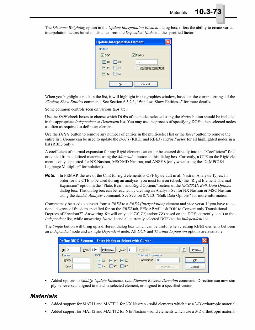
Materials 10.3-73
The Distance Weighting option in the Update Interpolation Element dialog box, offers the ability to create varied interpolation factors based on distance from the Dependent Node and the specified factor
When you highlight a node in the list, it will highlight in the graphics window, based on the current settings of the Window, Show Entities command. See Section 6.3.2.3, "Window, Show Entities..." for more details.
Some common controls seen on various tabs are:
Use the DOF check boxes to choose which DOFs of the nodes selected using the Nodes button should be included in the appropriate Independent or Dependent list. You may use the process of specifying DOFs, then selected nodes as often as required to define an element.
Use the Delete button to remove any number of entries in the multi-select list or the Reset button to remove the entire list. Update can be used to update the DOFs (RBE1 and RBE3) and/or Factor for all highlighted nodes in a list (RBE3 only).
A coefficient of thermal expansion for any Rigid element can either be entered directly into the “Coefficient” field or copied from a defined material using the Material... button in this dialog box. Currently, a CTE on the Rigid ele-ment is only supported for NX Nastran, MSC/MD Nastran, and ANSYS (only when using the “2..MPC184 Lagrange Multiplier” formulation).
Convert may be used to convert from a RBE2 to a RBE3 (Interpolation) element and vice versa. If you have rota-tional degrees of freedom specified for on the RBE2 tab, FEMAP will ask “OK to Convert only Translational Degrees of Freedom?”. Answering Yes will only add TX, TY, and/or TZ (based on the DOFs currently “on”) to the Independent list, while answering No will send all currently selected DOFs to the Independent list.
The Single button will bring up a different dialog box which can be useful when creating RBE2 elements between an Independent node and a single Dependent node. All DOF and Thermal Expansion options are available.
• Added options to Modify, Update Elements, Line Element Reverse Direction command. Direction can now sim-ply be reversed, aligned to match a selected element, or aligned to a specified vector.
Materials• Added support for MAT11 and MATT11 for NX Nastran - solid elements which use a 3-D orthotropic material.
• Added support for MAT12 and MATT12 for NEi Nastran - solid elements which use a 3-D orthotropic material.
Note: In FEMAP, the use of the CTE for rigid elements is OFF by default in all Nastran Analysis Types. In order for the CTE to be used during an analysis, you must turn on (check) the “Rigid Element Thermal Expansion” option in the “Plate, Beam, and Rigid Options” section of the NASTRAN Bulk Data Options dialog box. This dialog box can be reached by creating an Analysis Set for NX Nastran or MSC Nastran using the Model, Analysis command. See Section 8.7.1.3, "Bulk Data Options" for more information.
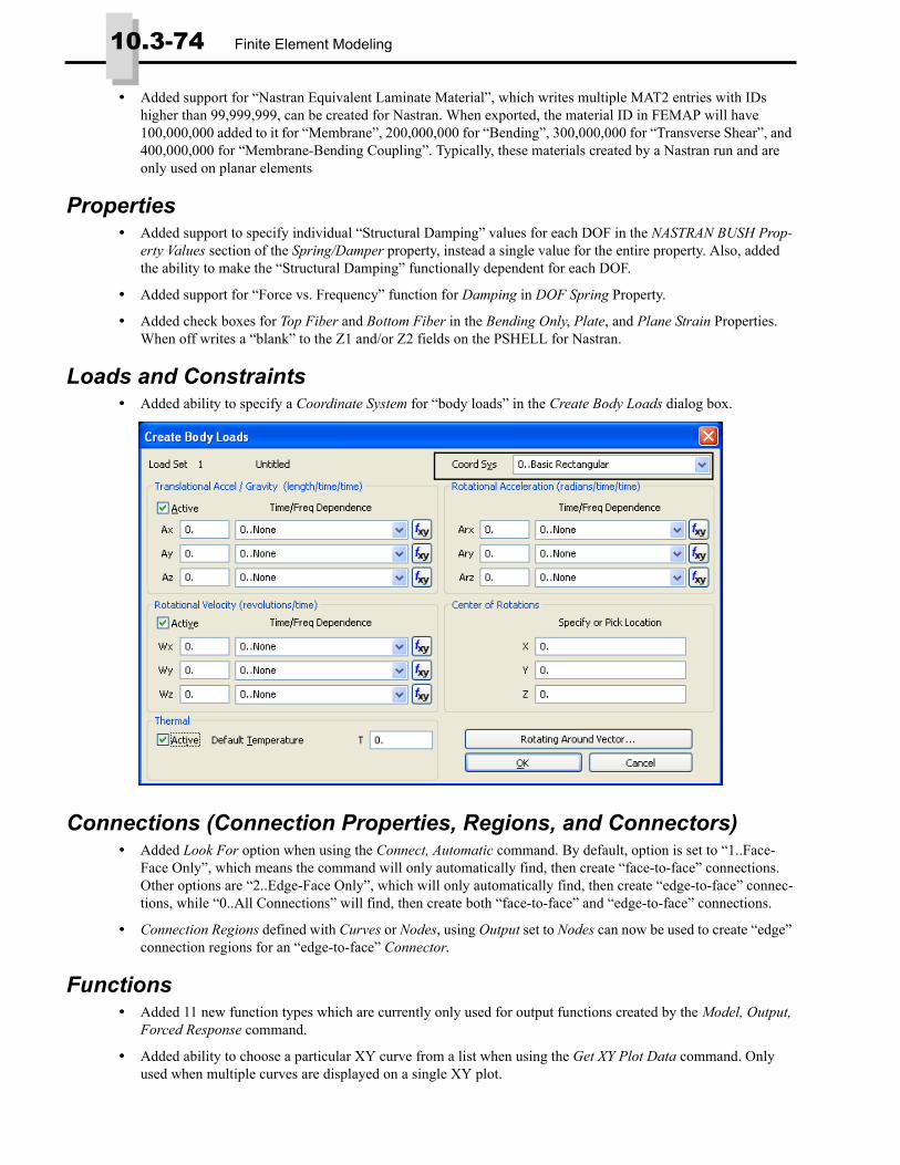
10.3-74 Finite Element Modeling
• Added support for “Nastran Equivalent Laminate Material”, which writes multiple MAT2 entries with IDs higher than 99,999,999, can be created for Nastran. When exported, the material ID in FEMAP will have 100,000,000 added to it for “Membrane”, 200,000,000 for “Bending”, 300,000,000 for “Transverse Shear”, and 400,000,000 for “Membrane-Bending Coupling”. Typically, these materials created by a Nastran run and are only used on planar elements
Properties• Added support to specify individual “Structural Damping” values for each DOF in the NASTRAN BUSH Prop-
erty Values section of the Spring/Damper property, instead a single value for the entire property. Also, added the ability to make the “Structural Damping” functionally dependent for each DOF.
• Added support for “Force vs. Frequency” function for Damping in DOF Spring Property.
• Added check boxes for Top Fiber and Bottom Fiber in the Bending Only, Plate, and Plane Strain Properties. When off writes a “blank” to the Z1 and/or Z2 fields on the PSHELL for Nastran.
Loads and Constraints• Added ability to specify a Coordinate System for “body loads” in the Create Body Loads dialog box.
Connections (Connection Properties, Regions, and Connectors)• Added Look For option when using the Connect, Automatic command. By default, option is set to “1..Face-
Face Only”, which means the command will only automatically find, then create “face-to-face” connections. Other options are “2..Edge-Face Only”, which will only automatically find, then create “edge-to-face” connec-tions, while “0..All Connections” will find, then create both “face-to-face” and “edge-to-face” connections.
• Connection Regions defined with Curves or Nodes, using Output set to Nodes can now be used to create “edge” connection regions for an “edge-to-face” Connector.
Functions• Added 11 new function types which are currently only used for output functions created by the Model, Output,
Forced Response command.
• Added ability to choose a particular XY curve from a list when using the Get XY Plot Data command. Only used when multiple curves are displayed on a single XY plot.

Views 10.3-75
Views• Added Connection and Coord Sys tabs to View, Visibility command.
In the Connection tab, you can toggle visibility on/off for both individual Connectors and Connection Regions.
In the Coord Sys tab, you can toggle on/off visibility for individual Coordinate Systems (user-defined only).
This table describes the functions performed by the command buttons when in the Connection or Coord Sys tab:
• View Options: Labels, Entities and Color category: Added Curve/Surface Directions option controls the dis-play of Parametric Directions of Curves and/or Surfaces. Replaces the Curve and Surface Accuracy option found in the Tools and View Style category in previous versions.
• View Options: Tools and View Style category: Clipping Planes option renamed Group Clipping Planes to differ-entiate between the clipping planes used in groups and the new Model Clipping Plane.
• View Options: Tools and View Style category: Added Model Clipping Plane option
This option can be used to set up a clipping pane that affects all entities in the model, without the use of any groups. To use the Model Clipping Plane, check the Enable option and select an option for Clipped Side (Positive or Nega-tive). When Clipped Side is set to Positive, ALL entities on the Positive side of the defined plane, based on normal direction, will be removed from the graphics window. Negative removes entities on the other side of the plane.
The default Model Clipping Pane for all new models is the Global YZ Plane in the Basic Rectangular coordinate system. If you want to change the plane, click the Clipping Plane button and use the Plane Locate - Define Clip-ping Plane dialog box.
When the Model Clipping Plane is “enabled”, the plane can be dynamically moved perpendicular to the defined plane by holding down the “Alt” key and spinning the Mouse Wheel backward or forward.
Entity/Label Button FunctionAll On “Checks” boxes for ALL Connectors and Connection Regions or Coordinate Sys-
tems in the list.All Off “Unchecks” boxes for ALL Connectors and Connection Regions or Coordinate Sys-
tems in the list.Selected On “Checks” boxes of highlighted Connectors/Connection Regions or Coordinate Sys-
tems in the list.Selected Off “Unchecks” boxes of highlighted Connectors/Connection Regions or Coordinate
Systems in the list.Selected Only “Checks” boxes of highlighted Connectors/Connection Regions or Coordinate Sys-
tems in the list, while “unchecking” boxes of Connectors/Connection Regions or Coordinate Systems which are not currently highlighted.
Note: If the Model Clipping Plane passes through the middle of an entity, such as a surface or element, a “par-tial entity” will be displayed. Also, entities will not appear “capped” based on the plane, so it is normal for entities to appear “hollow”.
Geometry displayed in “Wireframe”Cube with Sphere removedPlane not “Enabled”
Geometry displayed in “Solid”Plane “Enabled”Clipping Side set to “Positive”
Mesh displayed in “Solid”Plane moved to an XY PlaneClipping Side set to “Negative”

10.3-76 Finite Element Modeling
• View Options: PostProcessing category: Contour/Criteria Levels option. Modified and added options under Set Levels for Standard Colors.
Standard Colors
There are 5 options in the Standard Colors section:
Standard - uses Red for highest value and Magenta for the lowest level (Default)
No Magenta - uses Red for the highest value, but uses Dark Blue for the lowest value instead of Magenta. This is typical of several other Finite Element Analysis programs.
Temperature - uses White for the highest value (i.e., “White Hot”), Dark Blue for the lowest levels, and Red/Orange/Yellow as temperatures increase.
Red Yellow Green - uses Red for highest levels, Green for lowest levels, and Yellow for the middle.
Gray - uses Light Gray for the highest value and Dark Gray for the lowest value (i.e., Monochrome). You may want to do this prior to choosing the File, Print command if you are printing to a monochrome printer.
• View Options: PostProcessing category: Contour Type option. Added “2..Match Output” option to Contour Type list. When option is selected, nodal output data will be plotted as a Nodal Contour, while elemental output data will be plotted as an Elemental Contour.
• View Options: PostProcessing category: Beam Diagram option. Added Scale % option to scale beam diagrams.
Output and Post-Processing• Added "Include Max/Min Absolute Value" option to the List, Output, Summary To Data Table command. If
Include Max/Min Absolute Value is checked, then additional columns will be created displaying max/min val-ues created using the absolute value of the data
• Updated View, Advanced Post, Contour Model Data command to plot “Element Quality” values on elements as a contour or criteria plot.
• Updated Select XY Curve Data dialog box of View, Select command to use drop-down lists to select Output Sets for From and To in the Show Output Sets section instead of entering an integer value.
Note: You can specify a “Standard Colors” option for all new models using the File, Preferences command. Click the View tab, then choose an option from the “Contour Palette” drop-down in the Options section. See File, Preferences for more information.
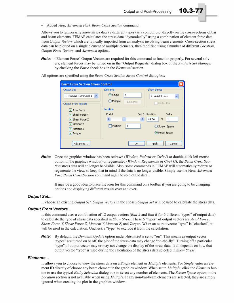
Output and Post-Processing 10.3-77
• Added View, Advanced Post, Beam Cross Section command.
Allows you to temporarily Show Stress data (8 different types) as a contour plot directly on the cross-sections of bar and beam elements. FEMAP calculates the stress data “dynamically” using a combination of element force data from Output Vectors which are typically imported from an analysis involving beam elements. Cross-section stress data can be plotted on a single element or multiple elements, then modified using a number of different Location, Output From Vectors, and Advanced options.
All options are specified using the Beam Cross Section Stress Control dialog box
Output Set...... choose an existing Output Set. Output Vectors in the chosen Output Set will be used to calculate the stress data.
Output From Vectors...... this command uses a combination of 12 output vectors (End A and End B for 6 different “types” of output data) to calculate the type of stress data specified in Show Stress. These 6 “types” of output vectors are Axial Force, Shear Force Y, Shear Force Z, Moment Y, Moment Z, and Torque. When an output vector “type” is “checked”, it will be used in the calculation. Uncheck a “type” to exclude it from the calculation.
Elements...... allows you to choose to view the stress data on a Single element or Multiple elements. For Single, enter an ele-ment ID directly of choose any beam element in the graphics window. When set to Multiple, click the Elements but-ton to use the typical Entity Selection dialog box to select any number of elements. The Screen Space option in the Location section is not available when using Multiple. If any non-bar/beam elements are selected, they are simply ignored when creating the plot in the graphics window.
Note: “Element Force” Output Vectors are required for this command to function properly. For several solv-ers, element forces may be turned on in the “Output Requests” dialog box of the Analysis Set Manager by checking the Force check box in the Elemental section.
Note: Once the graphics window has been redrawn (Window, Redraw or Ctrl+D or double-click left mouse button in the graphics window) or regenerated (Window, Regenerate or Ctrl+G), the Beam Cross Sec-tion stress data will no longer be visible. Also, some commands in FEMAP will automatically redraw or regenerate the view, so keep that in mind if the data is no longer visible. Simply use the View, Advanced Post, Beam Cross Section command again to re-plot the data.
It may be a good idea to place the icon for this command on a toolbar if you are going to be changing options and displaying different results over and over.
Note: By default, the Dynamic Update option under Advanced is set to “on”. This means as output vector “types” are turned on or off, the plot of the stress data may change “on-the-fly”. Turning off a particular “type” of output vector may or may not change the display of the stress data. It all depends on how that output vector “type” is used during the calculation of the stress data selected in Show Stress.
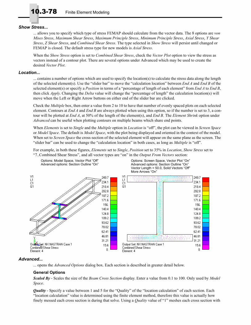
10.3-78 Finite Element Modeling
Show Stress...... allows you to specify which type of stress FEMAP should calculate from the vector data. The 8 options are von Mises Stress, Maximum Shear Stress, Maximum Principle Stress, Minimum Principle Stress, Axial Stress, Y Shear Stress, Z Shear Stress, and Combined Shear Stress. The type selected in Show Stress will persist until changed or FEMAP is closed. The default stress type for new models is Axial Stress.
When the Show Stress option is set to Combined Shear Stress, check the Vector Plot option to view the stress as vectors instead of a contour plot. There are several options under Advanced which may be used to create the desired Vector Plot.
Location...... contains a number of options which are used to specify the location(s) to calculate the stress data along the length of the selected element(s). Use the “slider bar” to move the “calculation location” between End A and End B of the selected element(s) or specify a Position in terms of a “percentage of length of each element” from End A to End B, then click Apply. Changing the Delta value will change the “percentage of length” the calculation location(s) will move when the Left or Right Arrow buttons on either end of the slider bar are clicked.
Check the Multiple box, then enter a value from 2 to 10 to have that number of evenly spaced plots on each selected element. Contours at End A and End B are always plotted when using this option, so if the number is set to 3, a con-tour will be plotted at End A, at 50% of the length of the element(s), and End B. The Element Shrink option under Advanced can be useful when plotting contours on multiple beams which share end points.
When Elements is set to Single and the Multiple option in Location is “off”, the plot can be viewed in Screen Space or Model Space. The default is Model Space, with the plot being displayed and oriented in the context of the model. When set to Screen Space the cross-section of the selected element will appear on the same plane as the screen. The “slider bar” can be used to change the “calculation location” in both cases, as long as Multiple is “off”.
For example, in both these figures, Elements set to Single, Position set to 35% in Location, Show Stress set to “7..Combined Shear Stress”, and all vector types are “on” in the Output From Vectors section:
Advanced...... opens the Advanced Options dialog box. Each section is described in greater detail below.
General OptionsScaled By - Scales the size of the Beam Cross Section display. Enter a value from 0.1 to 100. Only used by Model Space.
Quality - Specify a value between 1 and 5 for the “Quality” of the “location calculation” of each section. Each “location calculation” value is determined using the finite element method, therefore this value is actually how finely messed each cross section is during that solve. Using a Quality value of “1” meshes each cross section with
Options: Model Space, Vector Plot “Off” Options: Screen Space, Vector Plot “On”Advanced options: Section Outline “On”Vector Length = 50.0, Solid Vectors “Off”
Advanced options: Section Outline “On”
More Arrows “On”

Output and Post-Processing 10.3-79
the least amount of elements, but takes the least amount of time to calculate the values at each section. Entering a value of “5” will use the most elements and take the most time to solve.
Dynamic Update - On by default. When “on”, all changes made to options or location occur “on-the-fly”. When “off”, the Apply button must be clicked to make changes to the display.
Element Shrink - Shrinks the distance where a Beam Cross Section contour may be plotted along the length of an element, to a percentage of actual element length. This percentage is set using the “Shrink To %” field of the Shrink Elements option found in the View, Options command. Useful when using the Multiple option in Location and ele-ments share end points.
Section Outline - When “on”, displays an outline around all Beam Cross Section contour plots in the model, match-ing the outline of each section. Click Palette button to choose the outline color from the Color Palette dialog box. Especially helpful when Element - Orientation/Shape option in View, Options command is set to an option which does not show bar/beam element cross sections.
For example, in both these figures, Elements set to Single, Multiple option “on” and set to “3” in Location , Show Stress set to “4..Axial Stress”, and all vector types are “on” in the Output From Vectors section
Contour Legend Max/Min OptionsInclude End Stresses - On by default. When “on”, the max/min values of the Contour Legend are calculated using ALL locations of the selected elements. The Contour Legend does NOT change as the Position is changed and the displayed max/min values are NOT dependent on the current Position set in Location.
When “off”, the max/min values of the Contour Legend are calculated using the current location only of the selected element(s). When Dynamic Update is “on”, the Contour Legend will dynamically change as the Position is changed, thus making the range between max/min values smaller. A smaller range between max/min values combined with the same number of levels in the Contour Legend, yields a contour plot with more color variation for a particular location.
Note: You may want to turn Dynamic Update “off” if a large number of elements have been selected using Multiple option for Elements. That way, a number of options can be changed and the plot updated only once instead of every time an option is changed.
Default view with beam element cross sections displayed Advanced Options: Scaled By = 1.5Element Shrink “on”, Section Outline “on”
Include End Stresses is “on” Include End Stresses is “off”

10.3-80 Finite Element Modeling
Override - Turn this option “on” to override calculation of Max/Min values for the Contour Legend and instead simply use user-specified values for Min and Max. Include End Stresses option does nothing when this is “on”.
Vector Plot OptionsVector Length - Specify a value between 0.1 and 400, with 0.1 representing the shortest vectors. Default is 40.
Solid Vector - When “on”, vectors are displayed as Solid Vectors. When “off”, vectors appear as lines.
More Arrows - When “on”, “more vectors” will be displayed. If you need arrows near the outline of the plot, this option should be used.
• Added Model, Output, Forced Response command.
Calculates additional output using the results of a modal analysis as a basis. The values and type of the calculated “Output” depends on a number of “Inputs” and options specified by the user. This “Output” corresponds to results typically recovered from a “Frequency Response” analysis.
All “Input” is entered in the Forced Response Analysis dialog box:
The dialog box consists of 4 sections used which allow the user to enter specific “input”. Each section is important for generating the intended results:
DampingThis section controls the Damping values used in the calculation. A function MUST be specified for the Modal Damping Table, while the Overall Structural Damping value is optional.
Overall Structural Damping - “off” by default. When “on” this value provides overall structural damping for the model. Values should be entered between 0.00 and 1.00. A typical value to use is 2.0 * (critical damping ratio). This is equivalent to PARAM,G in Nastran solvers.
Note: When creating a Vector Plot, the default options may or may not produce what is considered a “useful” plot for all users. To create a “custom” Vector Plot try different combinations of the Vector Plot Options. This may take a few iterations.
Note: The user interface of the Forced Response command was designed using options for frequency response found in Nastran solvers. For Nastran users, the “equivalent” Nastran entry has been pro-vided in the documentation as a reference.

Output and Post-Processing 10.3-81
Modal Damping Table - A Model Damping Table is required and must be a FEMAP function with type set to “6..Structural Damping vs. Freq”, “7..Critical Damp vs. Freq”, or “Q Damping vs. Freq”. This function should span the frequency range of interest for the analysis. This is equivalent to TABDMP1 in Nastran solvers. If a function has not be previously defined, click the “Function” icon button to define one without having to leave the command.
Additionally, the values in the Model Damping Table can be treated as Viscous (default) or Structural. Setting the value to Structural is equivalent to using PARAM,KDAMP,-1 in Nastran solvers.
LoadingThis section contains one drop-down control which is used to select an existing Load Set from the model. A Load Set MUST be selected. Many times, a simple “Unit Load” in a particular direction is adequate, although this is cer-tainly not guaranteed to provide the desired results in all cases. For a Force “Unit Load”, this would create a DLOAD Case Control, along with RLOAD2, FORCE, DLOAD, and TABLED2 bulk data entries.
ModesChoose which modal Output Set(s) should be included when generating the additional output. Only Output Sets containing results from a modal analysis are available for selection and at least one Output Set from the Modes list must be selected. Along with being used to calculate the additional output, only the selected Modes will be used when certain Types of “frequency lists” are created. This is explained in greater detail in the Frequencies section.
FrequenciesAllows you to specify ranges of “Solution Frequencies” to use in the calculation of the additional output data. To define a frequency range, click the Create button. This will display the Define Frequency List dialog box.
Once a “Frequency List” has been created, it will appear in the Frequencies list. It will appear in this form:
List ID..(Frequency List Type): (Lower bound of frequency range) to (Upper bound of frequency range).
Check the box next to a particular “frequency list” to have the values used as “Solution Frequencies”. Any number of different “frequency lists” can be used. Highlight a “frequency list” and click Modify to bring up the Define Fre-quency List dialog box for that list, or click Delete to remove the highlighted “frequency list”. Click Preview to see the list of actual “Solution Frequencies”.
Define Frequency List dialog box:The Options in the Define Frequency List dialog box change based on the specified Type. There are 6 Types of “Frequency Lists” which can be created, each corresponding to a FREQi bulk data entry for Nastran.
Each Type is described below:
FREQ - Enter Frequency 1 (first in range), Frequency 2 (last in range), and an Increment (value entered in terms of frequency), then click Add Multiple button to add them to the Values list. For example Frequency 1 = 20, Fre-quency 2 = 100, and Increment = 20 would produce a list with values of 20, 40, 60, 80, and 100. Also, individual frequencies can added to the Values list by entering a value into the field below the list , then clicking the Add but-ton. Individual values may be deleted by selecting them one at a time in the Values list, then clicking Delete, while pressing Reset will clear the entire list. Copy will place the entire Values list on the clipboard, while Paste will fill the list with values from the clipboard.
FREQ1 - Enter Frequency 1 (first in range), Increment (value entered in terms of frequency), and Number (how many times to repeat the Increment), then click OK.
For example Frequency 1 = 20, Increment = 20, and Number = 5 would produce a list with values of 20, 40, 60, 80, 100, and 120.
FREQ2 - Enter Frequency 1 (first in range), Frequency 2 (last in range), and Number (how many logarithmic inter-vals within the range), then click OK.
For example Frequency 1 = 20, Frequency 2 = 100, and Number = 4 would produce a list with values of 20, 29.907, 44.7214, 66.874, and 100.
FREQ3 - Enter Frequency 1 (first in range), Frequency 2 (last in range), Number (number of excitation frequencies between two modal frequencies, value includes both modal frequencies), and Cluster (factor used for “clustering”
Note: For most Types, the Preview button in the Frequencies section of the Forced Response Analysis dialog box is the only way to see the actual values which will be used for calculations.
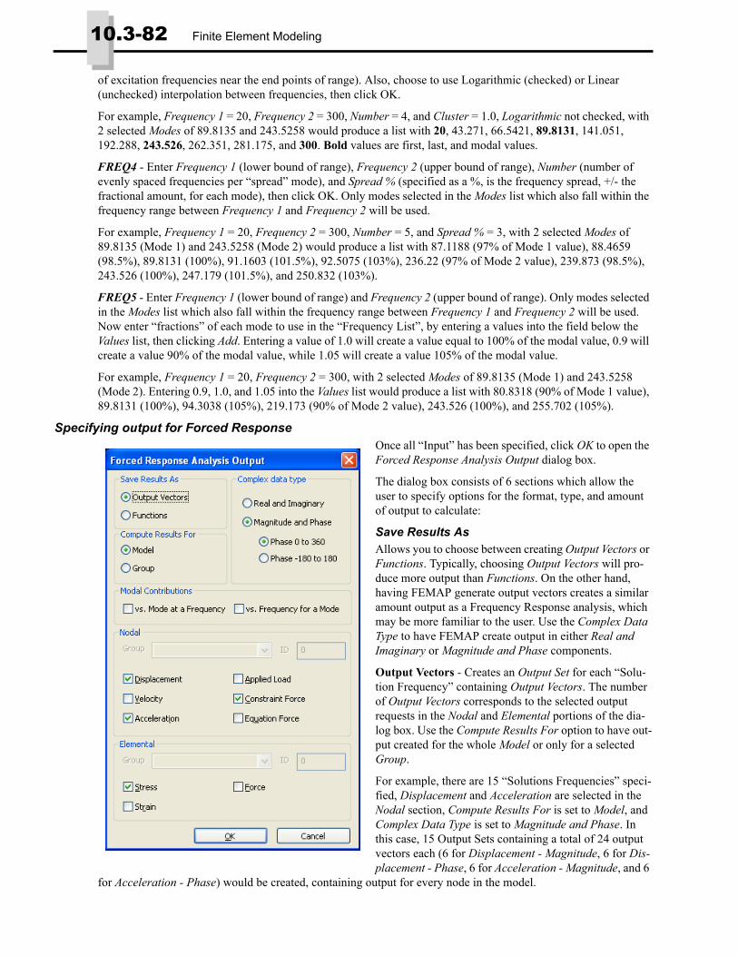
10.3-82 Finite Element Modeling
of excitation frequencies near the end points of range). Also, choose to use Logarithmic (checked) or Linear (unchecked) interpolation between frequencies, then click OK.
For example, Frequency 1 = 20, Frequency 2 = 300, Number = 4, and Cluster = 1.0, Logarithmic not checked, with 2 selected Modes of 89.8135 and 243.5258 would produce a list with 20, 43.271, 66.5421, 89.8131, 141.051, 192.288, 243.526, 262.351, 281.175, and 300. Bold values are first, last, and modal values.
FREQ4 - Enter Frequency 1 (lower bound of range), Frequency 2 (upper bound of range), Number (number of evenly spaced frequencies per “spread” mode), and Spread % (specified as a %, is the frequency spread, +/- the fractional amount, for each mode), then click OK. Only modes selected in the Modes list which also fall within the frequency range between Frequency 1 and Frequency 2 will be used.
For example, Frequency 1 = 20, Frequency 2 = 300, Number = 5, and Spread % = 3, with 2 selected Modes of 89.8135 (Mode 1) and 243.5258 (Mode 2) would produce a list with 87.1188 (97% of Mode 1 value), 88.4659 (98.5%), 89.8131 (100%), 91.1603 (101.5%), 92.5075 (103%), 236.22 (97% of Mode 2 value), 239.873 (98.5%), 243.526 (100%), 247.179 (101.5%), and 250.832 (103%).
FREQ5 - Enter Frequency 1 (lower bound of range) and Frequency 2 (upper bound of range). Only modes selected in the Modes list which also fall within the frequency range between Frequency 1 and Frequency 2 will be used. Now enter “fractions” of each mode to use in the “Frequency List”, by entering a values into the field below the Values list, then clicking Add. Entering a value of 1.0 will create a value equal to 100% of the modal value, 0.9 will create a value 90% of the modal value, while 1.05 will create a value 105% of the modal value.
For example, Frequency 1 = 20, Frequency 2 = 300, with 2 selected Modes of 89.8135 (Mode 1) and 243.5258 (Mode 2). Entering 0.9, 1.0, and 1.05 into the Values list would produce a list with 80.8318 (90% of Mode 1 value), 89.8131 (100%), 94.3038 (105%), 219.173 (90% of Mode 2 value), 243.526 (100%), and 255.702 (105%).
Specifying output for Forced ResponseOnce all “Input” has been specified, click OK to open the Forced Response Analysis Output dialog box.
The dialog box consists of 6 sections which allow the user to specify options for the format, type, and amount of output to calculate:
Save Results AsAllows you to choose between creating Output Vectors or Functions. Typically, choosing Output Vectors will pro-duce more output than Functions. On the other hand, having FEMAP generate output vectors creates a similar amount output as a Frequency Response analysis, which may be more familiar to the user. Use the Complex Data Type to have FEMAP create output in either Real and Imaginary or Magnitude and Phase components.
Output Vectors - Creates an Output Set for each “Solu-tion Frequency” containing Output Vectors. The number of Output Vectors corresponds to the selected output requests in the Nodal and Elemental portions of the dia-log box. Use the Compute Results For option to have out-put created for the whole Model or only for a selected Group.
For example, there are 15 “Solutions Frequencies” speci-fied, Displacement and Acceleration are selected in the Nodal section, Compute Results For is set to Model, and Complex Data Type is set to Magnitude and Phase. In this case, 15 Output Sets containing a total of 24 output vectors each (6 for Displacement - Magnitude, 6 for Dis-placement - Phase, 6 for Acceleration - Magnitude, and 6
for Acceleration - Phase) would be created, containing output for every node in the model.
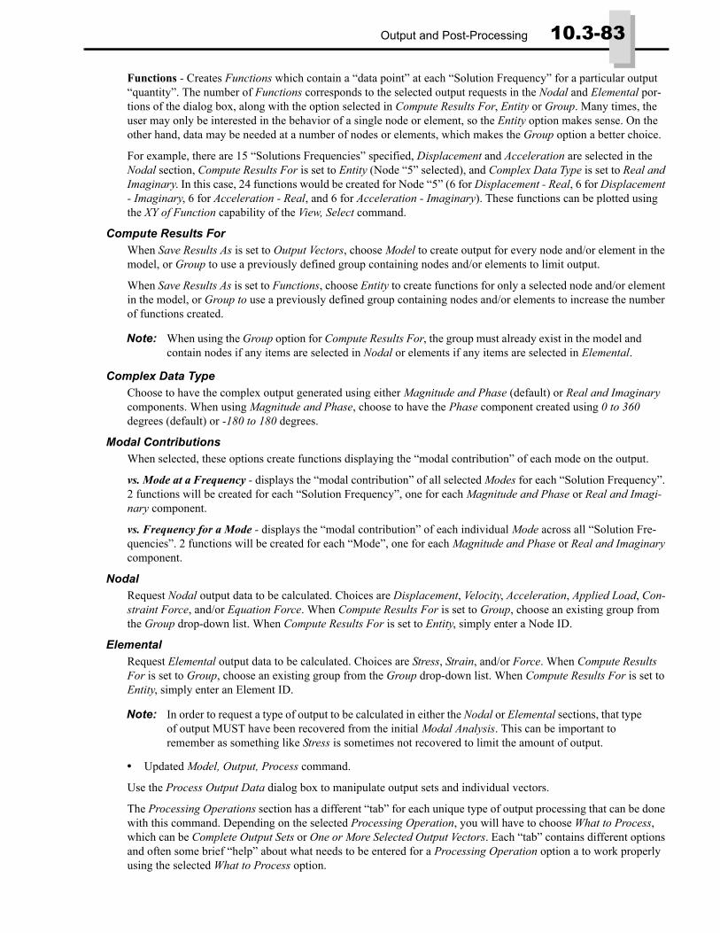
Output and Post-Processing 10.3-83
Functions - Creates Functions which contain a “data point” at each “Solution Frequency” for a particular output “quantity”. The number of Functions corresponds to the selected output requests in the Nodal and Elemental por-tions of the dialog box, along with the option selected in Compute Results For, Entity or Group. Many times, the user may only be interested in the behavior of a single node or element, so the Entity option makes sense. On the other hand, data may be needed at a number of nodes or elements, which makes the Group option a better choice.
For example, there are 15 “Solutions Frequencies” specified, Displacement and Acceleration are selected in the Nodal section, Compute Results For is set to Entity (Node “5” selected), and Complex Data Type is set to Real and Imaginary. In this case, 24 functions would be created for Node “5” (6 for Displacement - Real, 6 for Displacement - Imaginary, 6 for Acceleration - Real, and 6 for Acceleration - Imaginary). These functions can be plotted using the XY of Function capability of the View, Select command.
Compute Results ForWhen Save Results As is set to Output Vectors, choose Model to create output for every node and/or element in the model, or Group to use a previously defined group containing nodes and/or elements to limit output.
When Save Results As is set to Functions, choose Entity to create functions for only a selected node and/or element in the model, or Group to use a previously defined group containing nodes and/or elements to increase the number of functions created.
Complex Data TypeChoose to have the complex output generated using either Magnitude and Phase (default) or Real and Imaginary components. When using Magnitude and Phase, choose to have the Phase component created using 0 to 360 degrees (default) or -180 to 180 degrees.
Modal ContributionsWhen selected, these options create functions displaying the “modal contribution” of each mode on the output.
vs. Mode at a Frequency - displays the “modal contribution” of all selected Modes for each “Solution Frequency”. 2 functions will be created for each “Solution Frequency”, one for each Magnitude and Phase or Real and Imagi-nary component.
vs. Frequency for a Mode - displays the “modal contribution” of each individual Mode across all “Solution Fre-quencies”. 2 functions will be created for each “Mode”, one for each Magnitude and Phase or Real and Imaginary component.
NodalRequest Nodal output data to be calculated. Choices are Displacement, Velocity, Acceleration, Applied Load, Con-straint Force, and/or Equation Force. When Compute Results For is set to Group, choose an existing group from the Group drop-down list. When Compute Results For is set to Entity, simply enter a Node ID.
ElementalRequest Elemental output data to be calculated. Choices are Stress, Strain, and/or Force. When Compute Results For is set to Group, choose an existing group from the Group drop-down list. When Compute Results For is set to Entity, simply enter an Element ID.
• Updated Model, Output, Process command.
Use the Process Output Data dialog box to manipulate output sets and individual vectors.
The Processing Operations section has a different “tab” for each unique type of output processing that can be done with this command. Depending on the selected Processing Operation, you will have to choose What to Process, which can be Complete Output Sets or One or More Selected Output Vectors. Each “tab” contains different options and often some brief “help” about what needs to be entered for a Processing Operation option a to work properly using the selected What to Process option.
Note: When using the Group option for Compute Results For, the group must already exist in the model and contain nodes if any items are selected in Nodal or elements if any items are selected in Elemental.
Note: In order to request a type of output to be calculated in either the Nodal or Elemental sections, that type of output MUST have been recovered from the initial Modal Analysis. This can be important to remember as something like Stress is sometimes not recovered to limit the amount of output.
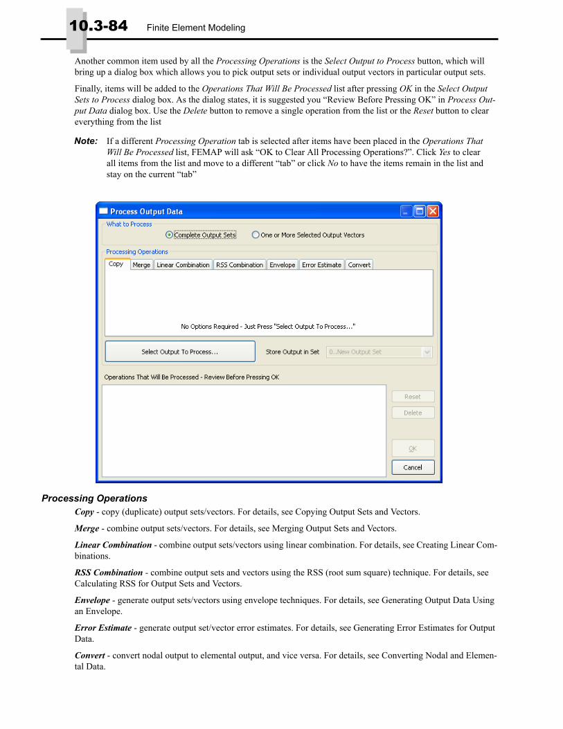
10.3-84 Finite Element Modeling
Another common item used by all the Processing Operations is the Select Output to Process button, which will bring up a dialog box which allows you to pick output sets or individual output vectors in particular output sets.
Finally, items will be added to the Operations That Will Be Processed list after pressing OK in the Select Output Sets to Process dialog box. As the dialog states, it is suggested you “Review Before Pressing OK” in Process Out-put Data dialog box. Use the Delete button to remove a single operation from the list or the Reset button to clear everything from the list
Processing OperationsCopy - copy (duplicate) output sets/vectors. For details, see Copying Output Sets and Vectors.
Merge - combine output sets/vectors. For details, see Merging Output Sets and Vectors.
Linear Combination - combine output sets/vectors using linear combination. For details, see Creating Linear Com-binations.
RSS Combination - combine output sets and vectors using the RSS (root sum square) technique. For details, see Calculating RSS for Output Sets and Vectors.
Envelope - generate output sets/vectors using envelope techniques. For details, see Generating Output Data Using an Envelope.
Error Estimate - generate output set/vector error estimates. For details, see Generating Error Estimates for Output Data.
Convert - convert nodal output to elemental output, and vice versa. For details, see Converting Nodal and Elemen-tal Data.
Note: If a different Processing Operation tab is selected after items have been placed in the Operations That Will Be Processed list, FEMAP will ask “OK to Clear All Processing Operations?”. Click Yes to clear all items from the list and move to a different “tab” or click No to have the items remain in the list and stay on the current “tab”

Output and Post-Processing 10.3-85
Performing Operations on Output Sets and VectorsThe general process for performing an operation on output sets or vectors is as follows:
1. Under Processing Operations, pick a tab, such as Copy. For some operations, you will want be select additional options in order to have the operation produce the desired output.
2. Under What to Process, choose Complete Output Sets or One or More Selected Output Vectors. When using the One or More Selected Output Vectors option, use the Store Output in Set drop-down to set a “destination” Output Set for the new output. The Complete Output Sets option is NOT available for Error Estimate or Convert.
3. Click Select Output to Process button. If Complete Output Sets is selected, a multi-select dialog box containing only the available Output Sets in the model will appear. If One or More Selected Output Vectors is selected, a larger dialog box containing a list of available Output Sets and Output Vectors, along with some additional options will be displayed. Once the desired output has been selected, click OK. See “Using Select Output to Pro-cess” for more information.
4. The Operations That Will Be Processed list is now filled with information about selected Processing Operation.5. You can continue to add Processing Operations of the same type to the Operations That Will Be Processed list.
When you are finished, click OK to process the operations and generate the new/modified output sets or vectors.
Using Select Output to ProcessThe only way to select which output sets and output vectors to consider when using the Model, Output, Process command is by clicking the Select Output to Process button. This displays one of two different Select Output Sets to Process dialog boxes, depending on the What to Process option.
When Complete Output Sets is selected, a multi-select dialog box containing only the existing output sets in the model will appear.
This is a “multi-select” dialog box, which can be used by selecting output sets by their title from a list. Holding down the “Ctrl” key will enable the selection of multiple output sets. Holding down “Shift” while picking a “first”, then a “last” output set will select a range.
The text field and “Filter” icon button at the bottom of the dialog box can be used to reduce the list based on the entered text. Enter more text and click the Filter again to create a smaller list. Click the “Clear Filter” icon button to return all output sets to the list.
The All button chooses all output sets currently in the list, so if the list is “filtered”, only those output sets will be highlighted. Click None to have no output sets selected in the list.

10.3-86 Finite Element Modeling
When One or More Selected Output Vectors is selected, a large dialog box containing a list of Output Sets in the model, Output Vectors from an output set specified using the From Output Set drop-down, and several other options will appear.
Along with checking and unchecking the boxes, you can also highlight the titles in the Output Sets or Output Vec-tors list, then click the Toggle Selected Sets or Toggle Selected Vectors buttons, respectively.
The list of Output Vectors displayed by default are always from the “Active” Output Set in the model. To see the list of Output Vectors from a different Output Set, simply select one from the From Output Set drop-down list.
If you check Select Similar Layer/Ply/Corner Vectors, you can select all similar data without worrying about checking all of the output vectors. For example, if you turn on this option, and select the vector "Plate Bot Von Mises Stress" (the centroidal Von Mises Stress at the bottom fiber of a plate/shell element), you will automatically also get the centroidal Von Mises Stress at the top fiber, and, if you have selected "Include Components/Corner Results", you will get the bottom and top Von Mises Stress at all of the element corners. Similarly, for laminate ele-ments, this option allows you to select results for all plys without having to select them manually. When using this option it does not matter which output vector location you choose, you will get the similar data for all locations.
Once finished, click OK and view the selected items in the Operations That Will be Processed list.
Copying Output Sets and VectorsUse Copy in the Processing Operations section to duplicate output vectors or entire output sets. An output set is always copied to a new output set. You can copy output vectors to an existing output set or to a new output set.
Using this OptionTo use this option, following the general steps in "Performing Operations on Output Sets and Vectors".
Merging Output Sets and VectorsUse Merge in the Processing Operations section to copy an output vector to another output set, or to combine two entire output sets, which may or may not have the same output vectors. Specify a Merge Approach:
If Do Not Overwrite Existing Output is selected, data in the Select Output to Process set will be skipped if it already exists in the set specified in Store Output in Set.
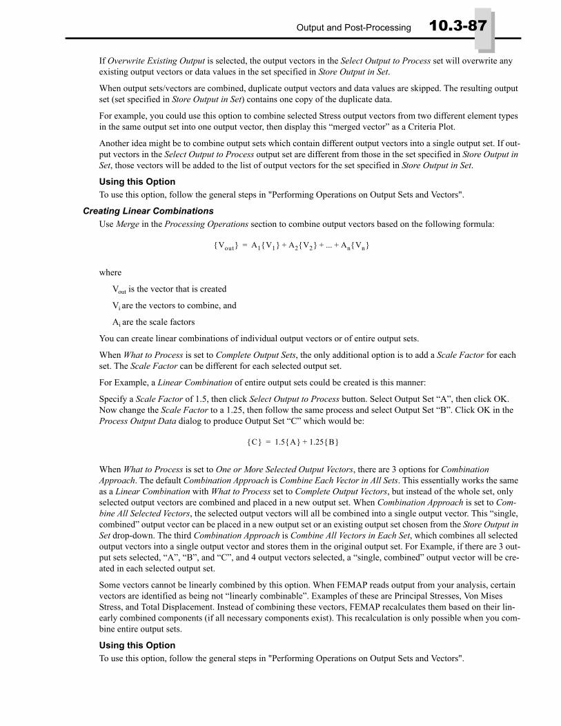
Output and Post-Processing 10.3-87
If Overwrite Existing Output is selected, the output vectors in the Select Output to Process set will overwrite any existing output vectors or data values in the set specified in Store Output in Set.
When output sets/vectors are combined, duplicate output vectors and data values are skipped. The resulting output set (set specified in Store Output in Set) contains one copy of the duplicate data.
For example, you could use this option to combine selected Stress output vectors from two different element types in the same output set into one output vector, then display this “merged vector” as a Criteria Plot.
Another idea might be to combine output sets which contain different output vectors into a single output set. If out-put vectors in the Select Output to Process output set are different from those in the set specified in Store Output in Set, those vectors will be added to the list of output vectors for the set specified in Store Output in Set.
Using this OptionTo use this option, follow the general steps in "Performing Operations on Output Sets and Vectors".
Creating Linear CombinationsUse Merge in the Processing Operations section to combine output vectors based on the following formula:
where
Vout is the vector that is created
Vi are the vectors to combine, and
Ai are the scale factors
You can create linear combinations of individual output vectors or of entire output sets.
When What to Process is set to Complete Output Sets, the only additional option is to add a Scale Factor for each set. The Scale Factor can be different for each selected output set.
For Example, a Linear Combination of entire output sets could be created is this manner:
Specify a Scale Factor of 1.5, then click Select Output to Process button. Select Output Set “A”, then click OK. Now change the Scale Factor to a 1.25, then follow the same process and select Output Set “B”. Click OK in the Process Output Data dialog to produce Output Set “C” which would be:
When What to Process is set to One or More Selected Output Vectors, there are 3 options for Combination Approach. The default Combination Approach is Combine Each Vector in All Sets. This essentially works the same as a Linear Combination with What to Process set to Complete Output Vectors, but instead of the whole set, only selected output vectors are combined and placed in a new output set. When Combination Approach is set to Com-bine All Selected Vectors, the selected output vectors will all be combined into a single output vector. This “single, combined” output vector can be placed in a new output set or an existing output set chosen from the Store Output in Set drop-down. The third Combination Approach is Combine All Vectors in Each Set, which combines all selected output vectors into a single output vector and stores them in the original output set. For Example, if there are 3 out-put sets selected, “A”, “B”, and “C”, and 4 output vectors selected, a “single, combined” output vector will be cre-ated in each selected output set.
Some vectors cannot be linearly combined by this option. When FEMAP reads output from your analysis, certain vectors are identified as being not “linearly combinable”. Examples of these are Principal Stresses, Von Mises Stress, and Total Displacement. Instead of combining these vectors, FEMAP recalculates them based on their lin-early combined components (if all necessary components exist). This recalculation is only possible when you com-bine entire output sets.
Using this OptionTo use this option, follow the general steps in "Performing Operations on Output Sets and Vectors".
Vout{ } A1 V1{ } A2 V2{ } ... An Vn{ }+ + +=
C{ } 1.5 A{ } 1.25 B{ }+=
10.3-88 Finite Element Modeling
Calculating RSS for Output Sets and VectorsUse the RSS Combination (root sum square) tab on the Process Output Data dialog box to calculate output vectors based on the following formula:
where
Vout is the vector that was created
Vi are the vectors to combine, and
Ai are the scale factors
You can calculate the root sum square for output vectors or for entire output sets.
The Scale Factor and Combination Approach sections are the same as Linear Combination. See Creating Linear Combinations for more information about these topics. A different Scale Factor may be set for each selected output set or vector.
Some vectors cannot be combined by this option. When FEMAP reads output from your analysis, certain vectors are identified as being not “linearly combinable”. Examples of these are Principal Stresses, Von Mises Stress, and Total Displacement. Instead of combining these vectors, FEMAP recalculates them based on their linearly com-bined components (if all necessary components exist). This recalculation is only possible when you combine entire output sets.
Using this OptionTo use this option, follow the general steps in "Performing Operations on Output Sets and Vectors".
Generating Output Data Using an EnvelopeUse the Envelope tab on the Process Output Data dialog box to choose a method for combining data. For each term (each vector or set that you want to envelope), you will select one of the three available methods in the Type sec-tion: Max Value, Min Value, or Max Absolute Value. The resulting envelope is based on the following formula:
where
Venv is the vector that is created
Vi are the vectors to envelope, and
F() is the max, min, or absmax function
You can choose to envelope entire output sets or individual output vectors. When using the One or More Selected Output Vectors option, select an Envelope Approach option to create different types of envelopes.
Using this OptionTo use this option, follow the general steps in "Performing Operations on Output Sets and Vectors".
For details on the Type options (Max Value, Min Value, or Max Absolute Value) options, see "How Envelope Works".
For details and Envelope Approach options, see When What to Process is set to One or More Selected Output Vec-tors.
For details on the Store Set/Location Info option, see "Requesting Set/Location Info".
How Envelope WorksThe first set or vector that you select is copied directly to the set or vector that will receive the enveloped data. If you specify additional vectors, the data from those vectors is combined with the existing enveloped data. There are three methods that you can use for the combination:
Vout{ } A1 V1{ }2 A2 V2{ }2 ... An Vn{ }2+ + +=
Venv{ } F Vn{ } F Vn 1–{ } F ... V1{ },( ),( ),( )=

Output and Post-Processing 10.3-89
Max Value enveloping: This method compares the envelope and added vector, and uses the maximum value of the node/element.
Min Value enveloping: This method compares the envelope and the added vector, and uses the minimum value of the node/element.
Max Absolute Value enveloping: This method compares the envelope and added vector, and uses the maximum absolute value of the node/element. The enveloped data will still contain both positive and negative values. The absolute value of the data is not saved; it is just used for the comparison.
For any method, if data does not exist for a node or element, in either the envelope or the additional vector, the result will simply be the value of the data that did exist.
When What to Process is set to Complete Output SetsSpecify a Type, such as Max Value, then select any number of output sets using the Select Output to Process button. This will always create a new output set that contains the maximum (or minimum, or absolute maximum) output values for every output vector at all nodes or elements in the original data. If the Store Set/Location Info option is “on”, an additional output set will be created. The output values at each node or element for every output vector in this additional output set are determined using the Output Set ID corresponding to the value for node or element used in the envelope output set.
For example, a Max Value envelope is created using 2 complete output sets (IDs “1” and “2”). Results exist for ele-ment “100” in both output sets and the Store Set/Location Info option is “on”. The value of von Mises Stress for element “100” is 120.00 in Output Set 1 and 110.00 in Output Set 2. In this case, the value for von Mises Stress for element “100” in the newly created “Envelope (Max 1,2)” output set would be 120.00 and the value in newly cre-ated “Envelope Set Info (Max 1,2)” output set would be 1. If Type was switched to Min Value, with all other inputs remaining the same, then the value for von Mises Stress for element “100” in the “Envelope (Min 1,2)” output set would be 110.00 and the value in “Envelope Set Info (Min 1,2)” would be 2.
When What to Process is set to One or More Selected Output VectorsSpecify a Type, such as Max Value, then select an Envelope Approach. There are three approaches that can be used for the combination:
Envelope All Selected Vectors: For simplicity, this description will use a single output set selected in the top por-tion of the Select Output Sets to Process dialog box. In this case, FEMAP simply creates a single vector to represent the envelope of all vectors selected in the bottom half Select Output Sets to Process of the dialog box. If the Store Set/Location Info option is “on”, an additional output vector or vectors may be created. Where the “enveloped” vector and additional “set/location” info vectors are stored after creation depends on the specified Create Enve-lopes options. When Within Output Sets is checked, the vector(s) will be stored in the output set selected in the top portion of the Select Output Sets to Process dialog box. If Across Output Sets is checked, the vector(s) will be stored in either a new output set or the set selected using the Store Output in Set drop-down. If both Create Enve-lopes options are selected, the data will be stored in both places
When multiple output sets are selected in the top portion of the Select Output Sets to Process dialog box, the Create Envelopes options actually change how the output data is enveloped.
When Within Output Sets is checked, only the output vectors within each selected output set will be enveloped with one another. The “enveloped” vector is stored in each individual output set. When Store Set/Location Info is “on”, a corresponding Location Info vector, containing only “Output Vector IDs”, will also be stored in each output set. For instance, if 3 output sets and 5 output vectors are selected, the 5 output vectors in Set “1” will be enveloped with one another, then the enveloped vectors will be stored in set “1”. Same process would occur for Sets “2” and “3”, therefore no data outside a selected output set is enveloped with data from any other output set.
When Across Output Sets is checked, all selected output vectors from ALL selected sets will be enveloped to create a single “enveloped” vector. This “enveloped” vector is stored in either a new output set or the set selected using the Store Output in Set drop-down. When Store Set/Location Info is “on”, a corresponding Set Info vector, contain-ing only “Output Set IDs”, and a Location Info vector, containing only “Output Vector IDs”, will also be stored in each output set. For instance, if 2 output sets and 5 output vectors are selected, with the Store Output in Set option set to “0..New Output Set”, then the 10 output vectors total (5 from each selected set) will all be enveloped with one another. The enveloped vector(s) will be stored in newly created Output Set “3”.
If both Create Envelopes options are selected, then an envelope for each selected output set and an additional one across all selected output sets will be created

10.3-90 Finite Element Modeling
Envelope All Locations For Each Vector: Used to create envelopes of a certain Type, such as Max Value, using all the “locations” of a particular output vector. “Locations” differ based on the shape and type of element. For instance, this option may be used to create a “Ply Summary” of results from an analysis involving laminate ele-ments. Other uses would be for determining the highest/lowest value from “top/bottom/middle” results on shell ele-ments, corners of solid or shell elements, both ends of a line element, or all stress recovery points a bar or beam. FEMAP will automatically determine which other vectors are needed to create an envelope of “locations” based on the vector(s) selected in the bottom portion of the Select Output Sets to Process dialog box. FEMAP will create an “enveloped” output vector for each different type (not each location) of selected output vector. Much like the Enve-lope All Selected Vectors approach, specifying the different Create Envelopes options and selection of a single out-put set or multiple output sets in the Select Output Sets to Process dialog box, can have a large affect on the data created in envelopes. See above for more details. In the case of a “ply summery”, only the output vector(s) of 1 “ply” need to be selected to create an envelope using this approach. Other examples include choosing only “top” or “bottom” vector(s) of shell element results, the output vector(s) on a single end of a line element (as long as results exist for both ends), vectors on a single corner for shell or solids (will include centroid value as well), or vectors of a single stress recovery point on bar/beam elements.
For example, if each ply of a laminate contained 10 separate output vectors, and Create Envelopes is set to Within Output Sets, then 10 “enveloped” vectors would be created “within” in each selected output set, based only on the output in each individual output set. When Store Set/Location Info is “on”, a corresponding Location Info output vector containing only “Ply IDs” for each “enveloped” vector will also be stored in each output set. In the same scenario, only using Create Envelopes set to Across Output Sets instead, 10 “enveloped” vectors would be created based on ALL selected output sets, then placed into either a new output set or an existing output set chosen using the Store Output in Set drop-down. When the Store Set/Location Info is “on” a corresponding Set Info output vector, containing only “Output Set IDs”, and a Location Info output vector, containing only “Ply IDs”, will be created and stored along with the “enveloped vectors”. If both Create Envelopes options are selected, then “location” envelope vectors will be created within each selected output set, while others are created for across ALL selected output sets.
Envelope Each Vector Independently: This is the default Envelope Approach and essentially does the same thing as an envelope of Complete Output Sets, except it only creates and stores output in a newly created ”Envelope Each Vector” output set for selected output vectors. Other differences include all enveloped output vectors will have IDs in the “User Data” range (9,000,000 and above) and when Store Set/Location Info option is “on”, simply creates additional vectors with titles starting with “Set Info” within the same ”Envelope Each Vector” output set instead of making a “Envelope Set Info” output set.
Requesting Set/Location InfoThe Store Set/Location Info option creates additional output, which offers details of the original “location” or out-put set of enveloped output data. When using Complete Output Sets, an additional output set containing all the same output vectors as the enveloped data output set will be created. When using One or More Selected Output Vectors, individual output vectors within sets that correspond to the enveloped data will be created. This provides an easy way to determine the worst case conditions for each output vector.
For Set Info output vectors, the output values will always be the ID of the output set where the enveloped data value originated.
When Envelope Approach is set to Envelope All Locations For Each Vector, Location Info vectors contain values in a particular format, based on the type and shape of the element:
“Ply Summary” of laminate elements - Value came from Ply ID = # (Integers Only)
“Top/Middle/Bottom” and “Corner” of shell elements - Value came from Top = -2, Middle = -1, or Bottom = -0. If value came from Corner # = 0.# (possible corner values 1-4). Thus, if displayed Location Info value is -2.3, this means the enveloped value came from the “Top, Corner 3” output vector.
“Corners” of solid elements - First digit in displayed value is always 1. Value came from Corner # = 0.# (1-8). Thus, if envelope value came from Corner 7 output vector (8-noded Brick), displayed value would be 1.7.
“End” and “Stress Recovery Point” of bar/beam elements - Value came from End A = 1 or End B = 2. If chosen vector contains Stress Recovery Point information, value came from Stress Recovery Point # = 0.0# (1-4). Thus, if envelope value came “Stress Recovery Point 4 of End B” output vector, displayed value would be 2.04.
Note: Because Set Info and Location Info values are usually the same for an entire element, a Criteria plot is often the best way to view these output vectors.
Output and Post-Processing 10.3-91
Generating Error Estimates for Output DataUse the Error Estimate tab on the Process Output Data dialog box to estimate the accuracy of the data in a selected output vector. This operation creates a new vector containing the estimate data. You can use any of the post-pro-cessing methods to display and evaluate the error estimate vector.
All finite element models and finite element analyses are engineering approximations. Depending upon how many elements you create, the shape of those elements, loading, boundary conditions, and many other factors, the accu-racy of your model/approximation can be very good or very bad. One of the main problems in using finite element results is that it is difficult to tell when the results truly represent reality. One historical method of verifying accu-racy is to build a second model that is more refined (has more elements), and check to see if you get the same or similar answers. If you do, the original approximation was reasonable. Unfortunately, this method takes a lot of work, and a lot of computer resources to run the additional analyses.
The error estimation operation attempts to quantify the validity of your approximations, without doing any addi-tional analysis or modeling. Even if the error estimations do not give you a definitive answer concerning the accu-racy of your model, they will certainly point out the portions of your model which need the most careful consideration. Typically, these will be areas where there are large gradients or localized changes in stress, displace-ment or other output quantities. These areas are usually critical in your design, and unless you properly refine the mesh, they can be poorly approximated.
The error estimates are based on these variations in output values. Ideally, within an element, or between elements connected to a common node, the variations in output should be relatively small. To the degree that these quantities vary, your model may not properly represent the true output state in that region. Error estimates show you how much variation is present throughout your model.
Using this OptionTo use this option, follow the general steps in "Performing Operations on Output Sets and Vectors". Remember, there is no way to choose and entire output set as the input for the Processing Operation and the resulting output vectors will always be stored within the selected “Original” output set(s).
Additional options for this operation include:
Choose an Error Method. For details, see "How Error Estimate Works" and “How Error Estimate Works”.
Use Output on Elements From, which lets you select the full model or a group. For details on selecting a group for this option, see “When to Use a Group” under the Converting Nodal and Elemental Data topic. While this topic does not specifically address error estimates, it uses output vectors and groups in a similar manner.
How Error Estimate WorksError estimates of nodal output data are calculated at the element centroids. Similarly, error estimates of elemental, centroidal output data are calculated at the nodes. The error estimates need to look at the variations in output data. An error estimate of nodal output data will be based on the gradients that data causes in each element. Hence the estimate is actually calculated for the element. An error estimate of elemental, centroidal output data is based on the differences that occur at the elemental boundaries. Specifically, FEMAP bases the calculations on the output values from all elements connected to a specific node. That is why the error estimates are formulated at the nodes for elemental data.
The calculation of error estimates for nodal output is fairly straightforward. The values at each node connected to an element are simply compared. Error estimates for elemental data are more complicated. They follow the same rules that FEMAP uses for the Convert option. Since this calculation is also done at nodes (element corners), FEMAP needs to use the output value at the appropriate element corner for each node. If you recover elemental corner output, FEMAP automatically uses these output values at each corner, even though you must select a cent-roidal output vector. If you do not recover corner output, FEMAP simply uses the centroidal value from the output vector that you selected.
You can choose any of six Error Methods to create the error estimate output data. All of them follow the procedures described above. The only difference between them is the formula used to calculate the estimate.

10.3-92 Finite Element Modeling
Max Difference Method
Difference from Average Method
% Max Difference Method
% Difference from Average Method
Normalized % Max Difference Method
Normalized % Difference from Average Method
In each of these calculations, the Min, Max and Avg values refer to the minimum, maximum, and average output values at the node or element where the error estimate is being calculated. The Vector Max values refer to the max-imum value for all nodes or elements in the output vector. You will notice that all error estimates are either zero or positive, since they all use the absolute value of the various factors.
The choice of an appropriate error estimation method largely depends on the conditions in your model. FEMAP will allow you to calculate as many error estimates as you want. You just have to use the Error Estimate option multiple times.
ValueMax Value– Min
MAX ValueMax ValueAvg– ValueMin ValueAvg–( , )
ValueMax ValueMin–ValueAvg
------------------------------------------------------- 100%×
MAX ValueMax ValueAvg– ValueMin ValueAvg–( , )ValueAvg
----------------------------------------------------------------------------------------------------------------------------------------- 100%×
ValueMax ValueMin–ValueVectorMax
------------------------------------------------------- 100%×
MAX ValueMax ValueAvg– ValueMin ValueAvg–( , )ValueVectorMax
----------------------------------------------------------------------------------------------------------------------------------------- 100%×

Output and Post-Processing 10.3-93
The following table lists the uses for each method..
Error Estimate ExamplesA few brief examples with hypothetical data will help to illustrate the various error estimates:
Suppose that you have output values surrounding some location (a node or element) that are 100, 100, 300, 300, and at another location you have 100, 100, 100, 500, and at a third location you have 1, 1, 3, 3. The following error estimates would be calculated:
You will notice that the two unnormalized percentage methods make no distinction between the first location with 100 and 300 output values and the last with 1 and 3. Also note how the Max Difference from Average method (and the corresponding normalized percentage method) highlights the middle position where all values are constant (100) except for the single 500 value. You will notice that the average values for the first and second output posi-tions are identical (200), even though they represent very different conditions. If you just look at contour or overall data, you will only see these averages.
Converting Nodal and Elemental DataUse the Convert tab on the Process Output Data dialog box to convert nodal output data to elemental data, and vice-versa. Data is simply converted from the selected output vector into a new vector of the opposite type. The title of the new vector will indicate that it is a converted vector, and will also show the ID of the original vector.
Some FEMAP post-processing options (displacements, animations) use nodal data, while others (criteria plots) use elemental data. No matter what post-processing option you choose, you can also choose any output vector - whether it contains nodal or elemental data. If the type of output you choose does not match the type required, FEMAP automatically converts the data every time it needs to display your model.
Method UsesMax Difference • Identifies largest gradients in portions of the model with larg-
est output values.• Identifies steepest gradients in the most critical portions of
the model.Difference from Average • Identifies areas with largest output values. Areas where only
one or a few values are different are accentuated.• Identifies only steepest non-uniform gradients (those that
vary in a single direction).% Max Difference Identifies same gradients as Max Difference, but does not distin-
guish between large and small output values. Use only if magni-tude of the output is less important than the changes in output.
% Difference from Average Identifies same gradients as Difference from Average, but does not distinguish between large and small output values. Use only if magnitude of the output is less important than the changes in output
Normalized % Max Differ-ence
Best at quantifying overall errors in areas with peak output val-ues.
Normalized % Difference from Average
Best at quantifying overall errors in areas with peak output val-ues.
Values Min Max Avg Max Diff
Max Diff from Avg
% Max Diff
% Diff from Avg
Nrm %
Max Diff
Nrm %
Diff from Avg
100,100,300,300
100 300 200 200 100 100% 50% 40% 20%
100,100,100,500
100 500 200 400 300 200% 150% 80% 60%
1, 1, 3, 3 1 3 2 2 1 100% 50% 0.4% 0.2%

10.3-94 Finite Element Modeling
When the display is updated, the converted data is discarded. Obviously, for large models, this can take some time. In these cases, you can manually convert the vector, then select the new, converted vector for post-processing. In either case, the results will be displayed identically; however, the converted vector will plot much more rapidly.
The converted output data may also be used to perform tasks such as listing stress output on nodes to the Data Table.
Using this OptionTo use this option, follow the general steps in "Performing Operations on Output Sets and Vectors". Remember, there is no way to choose and entire output set as the input for the Processing Operation and the resulting output vectors will always be stored within the selected “Original” output set(s).
• For details on the Conversion Approach options, see "How Convert Works".
• For details on Using Output on Elements From option, see “When to Use a Group”.
How Convert WorksWhenever you are using FEMAP to interpret output values, it is important to understand how your data is being manipulated, especially when you look at contour plots. It is easy to draw incorrect conclusions if you do not prop-erly understand what is being displayed.
Set the Conversion Approach to Average Values to use the “Averaged” values during the conversion. Set this to Maximum Values to use the “Maximum” values of the output during the conversion.
For more information on contour plots, see Section 8.2.2.2, "Selecting Data for a Deformed or Contour Style".
Converting Nodal Data to Elemental DataThe conversion process in this case is straightforward. Output values from all of the nodes referenced by an ele-ment are simply averaged (or max value is used) to compute the elemental output value. If data does not exist at one or more nodes, that node is skipped. It is not considered as a zero value; it is simply not considered in the aver-age.
Converting Elemental Data to Nodal DataThis conversion process is somewhat more complex. In general, FEMAP calculates the nodal output value by aver-aging the output values for all elements that reference that node. If you are converting an output vector that defines data at element centroids, and there is no similar data available at the element corners, the centroidal data will be used as the value at the node for that element. If you do have element corner data, however, the corner values at the node will be used in place of the centroidal value. In either case, you can choose to average the values from all ele-ments or take the maximum value.
When to Use a GroupIf you do not specify a group, the conversion process will use data from every node or element in your model. This is fine for many data types. For example, stresses in solid elements can often be converted this way.
In other cases, however, this type of conversion can lead to problems. For instance, suppose that you have a model of a box-shaped structure that is made of plate elements. Also, suppose that you need to convert elemental stresses to nodal stresses so that you can do a contour display. If you let FEMAP convert output from the entire model, dis-crepancies will be introduced along the edges and at the corners of the box. At these locations, elements from dif-ferent faces of the box join. If you convert the entire model, in-plane stresses from perpendicular faces will be averaged together. These stresses are, in fact, located in different planes, and should never be averaged. Instead, you should define a group that contains only the elements that make up a single side of the box. If you then select that group, FEMAP will only use the stresses on the elements in that face. No errors will be introduced at the edges or corners.
As in this example, you should always use a group when the conversion process would combine output from differ-ent directions or planes. You may also want to use groups to isolate elements that reference particular properties or materials. Depending on the type of data you are converting, combining data across cross-section or material boundaries may or may not be accurate. It depends on whether the data you are converting must satisfy equilibrium conditions across the boundary.

Geometry Interfaces 10.3-95
Geometry InterfacesThe following FEMAP interfaces have been updated to support newer geometry formats:
• Added support for reading IGES files with no “Start Section”.
For details, see “Geometry Interfaces” in the FEMAP User Guide.
Analysis Program InterfacesSeveral of the analysis program interfaces have been improved. These changes include:
• Analysis Set Manager Enhancements
• FEMAP Neutral File Interface
• NX Nastran Interface
• Nastran Interfaces (NX and MSC/MD)
• MSC/MD Nastran Interface
• NEi Nastran Interface
• ANSYS Interface
• ABAQUS Interface
• DYNA Interface
For details, see “Analysis Program Interfaces” in the FEMAP User Guide.
Analysis Set Manager Enhancements• Added “conditional text” to all Start Text and End Text buttons in Manual Control sections throughout the Anal-
ysis Set Manager.
When a button shows “Off”, nothing is entered in the Analysis Text window did when that Start Text or End Text button is clicked. When a button shows “On”, there is text that particular Analysis Text dialog box.
FEMAP Neutral File Interface• Updated Neutral Read and Write for v10.2 changes
NX Nastran Interface• Added support for BLSEG and BCPROPS to support edge-to-face glue.
FEMAP Interface Latest Supported VersionParasolid Parasolid 23.0Solid Edge Solid Edge with Synchronous Technology 3NX NX 7.5ACIS ACIS 21SolidWorks SolidWorks 2010

10.3-96 Finite Element Modeling
• Added support for the TSTART and ATSMASS options on NXSTRAT entry.
• Added support for Minimum Accleration (5th Line of NAVSHOCK File), Unit Conversion -Force (10th Line of NAVSHOCK File), and Unit Conversion - Acceleration (11th Line of NAVSHOCK File) options for DDAM analysis.
• Added support for MAT11 and MATT11 entries for 3D Orthotropic Materials when referenced by solid ele-ments.
• Added support PARAM,WMODAL
• Added support for ENFMOTN system cell. Value 0 = “Constraint Mode”, 1 = “Absolute”, 2 = “Absolute, Vis-cous Damping”.
• Added support for CPLSTN3, CPLSTN4, CPLSTN6, and CPLSTN8 Plane Strain Elements via formulation.
• Added support for CPLSTS3, CPLSTS4, CPLSTS6, and CPLSTS8 Plane Stress Elements via formulation.
• Added support for reading CDDATA from Mode Tracking Method 2. Also, fixed import of CDDATA when using Mode Tracking Method 1.
A number of bugs were corrected
For details, see “Analysis Program Interfaces” in the FEMAP User Guide.
Nastran Interfaces (NX and MSC/MD)• Added Defaults button to Nonlinear Control Options dialog box for Analysis Types “10..Nonlinear Static” and
“11..Nonlinear Transient Response”.
• Added support for Structural Damping on each DOF for PBUSH (GEi fields) and PBUSHT (TGEIDi fields)
• Added support for PARAM, KDAMP
• Added support for PARAM, FZERO
• Added support for PDAMPT
• Added support for “Fluid Nodes” by setting CD field of GRID entry to -1
• Added support for writing “blank” Z1 and//or Z2 fields to the PSHELL
• Added support for “Nastran Equivalent Laminate” material, which generates multiple MAT2 entries.
• Added read support for GROUNDCHECK and WEIGHTCHECK
• Added read support for FREQ1, FREQ2, FREQ3, and FREQ4 (only reads first 2 FREQi entries in input file)
• Changed “Bulk Data Delete” entry for restarts from “/,1,999,999” to “/,1,9,999,999”
A number of bugs were corrected
For details, see “Analysis Program Interfaces” in the FEMAP User Guide.
MSC/MD Nastran Interface• Added Support for PARAM, ENFMOTN. ABS = “Absolute”, REL = “Relative”.
A number of bugs were corrected.
For details, see “Analysis Program Interfaces” in the FEMAP User Guide.
NEi Nastran Interface• Added support for MAT12 and MATT12 entries for 3D Orthotropic Materials when referenced by solid ele-
ments.
• Removed default values from Nonlinear Control Options dialog box for Analysis Types “10..Nonlinear Static” and “11..Nonlinear Transient Response”
A number of bugs were corrected.
For details, see “Analysis Program Interfaces” in the FEMAP User Guide.
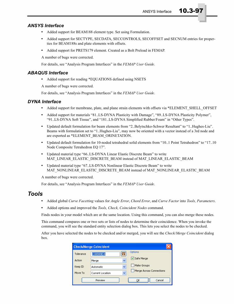
ANSYS Interface 10.3-97
ANSYS Interface• Added support for BEAM188 element type. Set using Formulation.
• Added support for SECTYPE, SECDATA, SECCONTROLS, SECOFFSET and SECNUM entries for proper-ties for BEAM188s and plate elements with offsets.
• Added support for PRETS179 element. Created as a Bolt Preload in FEMAP.
A number of bugs were corrected.
For details, see “Analysis Program Interfaces” in the FEMAP User Guide.
ABAQUS Interface• Added support for reading *EQUATIONS defined using NSETS
A number of bugs were corrected.
For details, see “Analysis Program Interfaces” in the FEMAP User Guide.
DYNA Interface• Added support for membrane, plate, and plane strain elements with offsets via *ELEMENT_SHELL_OFFSET
• Added support for materials “81..LS-DYNA Plasticity with Damage”, “89..LS-DYNA Plasticity Polymer”, “91..LS-DYNA Soft Tissue”, and “181..LS-DYNA Simplified Rubber/Foam” in “Other Types”.
• Updated default formulation for beam elements from “2..Belytschko-Schwer Resultant” to “1..Hughes-Liu”. Beams with formulation set to “1..Hughes-Liu”, may now be oriented with a vector instead of a 3rd node and are exported as *ELEMENT_BEAM_ORINETATION.
• Updated default formulation for 10-noded tetrahedral solid elements from “10..1 Point Tetrahedron” to “17..10 Node Composite Tetrahedron EQ 17”.
• Updated material type “66..LS-DYNA Linear Elastic Discrete Beam” to write MAT_LINEAR_ELASTIC_DISCRETE_BEAM instead of MAT_LINEAR_ELASTIC_BEAM
• Updated material type “67..LS-DYNA Nonlinear Elastic Discrete Beam” to write MAT_NONLINEAR_ELASTIC_DISCRETE_BEAM instead of MAT_NONLINEAR_ELASTIC_BEAM
A number of bugs were corrected.
For details, see “Analysis Program Interfaces” in the FEMAP User Guide.
Tools• Added global Curve Facetting values for Angle Error, Chord Error, and Curve Factor into Tools, Parameters.
• Added options and improved the Tools, Check, Coincident Nodes command.
Finds nodes in your model which are at the same location. Using this command, you can also merge these nodes.
This command compares one or two sets or lists of nodes to determine their coincidence. When you invoke the command, you will see the standard entity selection dialog box. This lets you select the nodes to be checked.
After you have selected the nodes to be checked and/or merged, you will see the Check/Merge Coincident dialog box.

10.3-98 Finite Element Modeling
FEMAP has two separate node merging algorithms, “Safe Merge” and “Original Merge”. The Safe Merge check box under Options selects which algorithm will be used (checked = Safe Merge, unchecked = Original Merge).
In the Check/Merge Coincident dialog box, specify a merge Tolerance. Nodes whose difference in locations are less than this distance are considered to be coincident. It is a good idea to set this to a small number relative to your model size. If desired, click the Measure Distance icon button to choose two locations from the screen to use as the Tolerance.
The Action drop-down list allows you to choose what will happen to any coincident nodes which are found.
If you want to eliminate the coincident nodes which are found, choose either Merge or Merge and List. .
If you want to only list the coincident nodes, choose List or Detailed List.
List - simply lists the nodes which would be merged based on the specified Tolerance value, along with the distance between the two nodes.
Detailed List - expands the list to include every pair of nodes that fall within the specified Tolerance, including nodes which will not be merged. Reasons nodes will not be merged include instances where nodes are on both sides of a Connector or merging the nodes would result in alteration or collapse of another element.
The Keep ID drop-down allows you to select which nodes will remain in the model after the nodes are merged.
There are four Keep ID options:
Automatic - merges nodes based on how the algorithm locates the coincident nodes and gives the user NO control of which nodes will be merged and kept.
Lower ID - for each set of coincident nodes, FEMAP will keep the node with the lowest ID numerically and merge any nodes coincident to the “lowest ID node”.
Higher ID - for each set of coincident nodes, FEMAP will keep the node with the highest ID numerically and merge any nodes coincident to the “highest ID node”.
Select Node(s) to Keep - allows you to specify a second list of nodes to check/keep against the list you originally specified. When using this option, after you press OK in Check/Merge Coincident dialog box, you will be asked for a second set of nodes. With the second set of nodes, you may choose nodes you want to remain in the model after the merging process. This option gives you a bit more control, specifically if you want to assure certain nodes will remain in the model.
After determining any number of nodes are within the specified Tolerance to one another, the Move To drop-down allows you to select where the “kept” node from any particular “set of nodes” will be located after the nodes are merged. If any nodes in each “set of nodes” cannot be merged to any of the other nodes for some reason, this is taken into consideration.
There are four Move To options:
Current Location - the “kept” node(s) will remain in their original locations.
Lower ID - the “kept” node(s) will be moved to the location of the node with the lowest ID for each “set of nodes”.
Note: “Safe Merge” is the default and should be used whenever possible. The only reason to use “Origi-nal Merge” is if you find an issue with “Safe Merge”. Also, when using “Original Merge”, the entire Move To drop-down list and the Detailed List option in the Action drop-down list are not available. All listing in “Original Merge” behaves like Detailed List in “Safe Merge”. Finally, “Original Merge” will be removed in a future version.
Note: FEMAP determines the default node merge tolerance based on overall model size. The number is 1/10000 of the “model box diagonal” (think of the model box being an invisible box that com-pletely encapsulates every entity in the model).
You can override the default node merge tolerance by specifying a value in Tools, Parameters. Simply change the Merge Tolerance option to “Specified” and enter a value. This value will be saved with your model.
Note: If knowing the IDs of the coincident nodes is NOT important, use Merge option, as it takes less time.
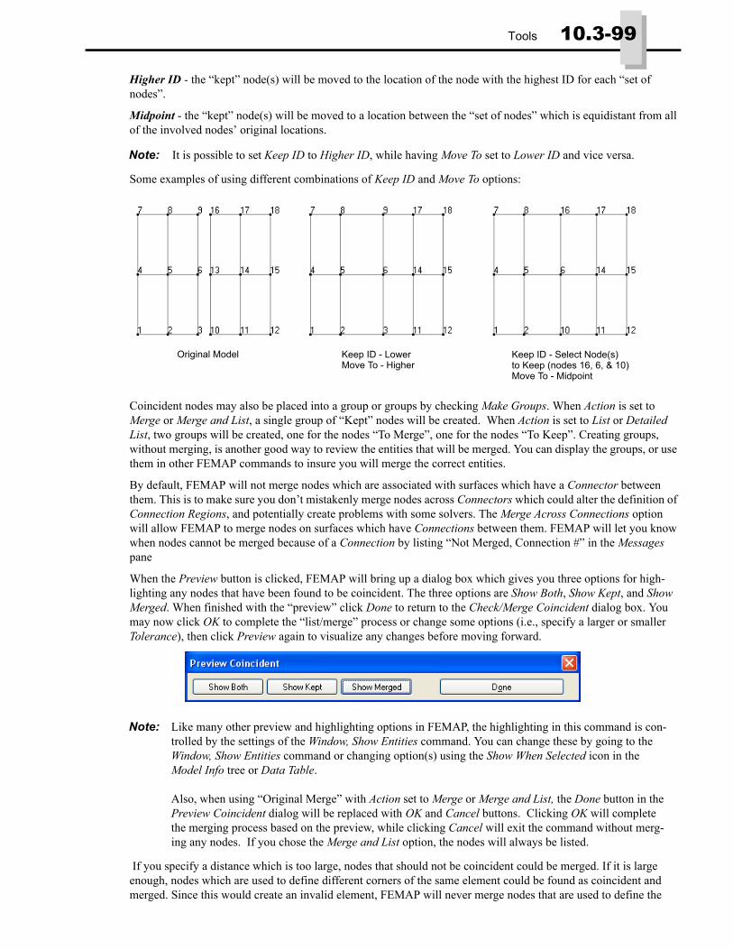
Tools 10.3-99
Higher ID - the “kept” node(s) will be moved to the location of the node with the highest ID for each “set of nodes”.
Midpoint - the “kept” node(s) will be moved to a location between the “set of nodes” which is equidistant from all of the involved nodes’ original locations.
Some examples of using different combinations of Keep ID and Move To options:
Coincident nodes may also be placed into a group or groups by checking Make Groups. When Action is set to Merge or Merge and List, a single group of “Kept” nodes will be created. When Action is set to List or Detailed List, two groups will be created, one for the nodes “To Merge”, one for the nodes “To Keep”. Creating groups, without merging, is another good way to review the entities that will be merged. You can display the groups, or use them in other FEMAP commands to insure you will merge the correct entities.
By default, FEMAP will not merge nodes which are associated with surfaces which have a Connector between them. This is to make sure you don’t mistakenly merge nodes across Connectors which could alter the definition of Connection Regions, and potentially create problems with some solvers. The Merge Across Connections option will allow FEMAP to merge nodes on surfaces which have Connections between them. FEMAP will let you know when nodes cannot be merged because of a Connection by listing “Not Merged, Connection #” in the Messages pane
When the Preview button is clicked, FEMAP will bring up a dialog box which gives you three options for high-lighting any nodes that have been found to be coincident. The three options are Show Both, Show Kept, and Show Merged. When finished with the “preview” click Done to return to the Check/Merge Coincident dialog box. You may now click OK to complete the “list/merge” process or change some options (i.e., specify a larger or smaller Tolerance), then click Preview again to visualize any changes before moving forward.
If you specify a distance which is too large, nodes that should not be coincident could be merged. If it is large enough, nodes which are used to define different corners of the same element could be found as coincident and merged. Since this would create an invalid element, FEMAP will never merge nodes that are used to define the
Note: It is possible to set Keep ID to Higher ID, while having Move To set to Lower ID and vice versa.
Note: Like many other preview and highlighting options in FEMAP, the highlighting in this command is con-trolled by the settings of the Window, Show Entities command. You can change these by going to the Window, Show Entities command or changing option(s) using the Show When Selected icon in the Model Info tree or Data Table.
Also, when using “Original Merge” with Action set to Merge or Merge and List, the Done button in the Preview Coincident dialog will be replaced with OK and Cancel buttons. Clicking OK will complete the merging process based on the preview, while clicking Cancel will exit the command without merg-ing any nodes. If you chose the Merge and List option, the nodes will always be listed.
Original Model Keep ID - LowerMove To - Higher
Keep ID - Select Node(s)to Keep (nodes 16, 6, & 10)Move To - Midpoint
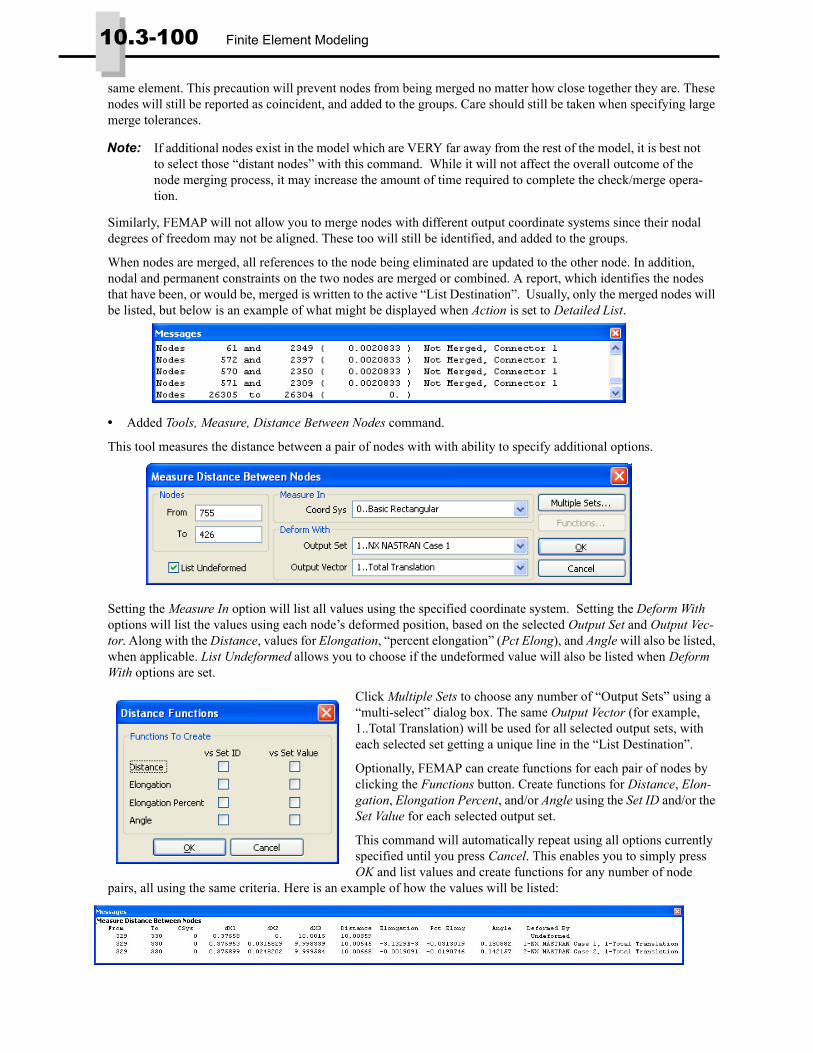
10.3-100 Finite Element Modeling
same element. This precaution will prevent nodes from being merged no matter how close together they are. These nodes will still be reported as coincident, and added to the groups. Care should still be taken when specifying large merge tolerances.
Similarly, FEMAP will not allow you to merge nodes with different output coordinate systems since their nodal degrees of freedom may not be aligned. These too will still be identified, and added to the groups.
When nodes are merged, all references to the node being eliminated are updated to the other node. In addition, nodal and permanent constraints on the two nodes are merged or combined. A report, which identifies the nodes that have been, or would be, merged is written to the active “List Destination”. Usually, only the merged nodes will be listed, but below is an example of what might be displayed when Action is set to Detailed List.
• Added Tools, Measure, Distance Between Nodes command.
This tool measures the distance between a pair of nodes with with ability to specify additional options.
Setting the Measure In option will list all values using the specified coordinate system. Setting the Deform With options will list the values using each node’s deformed position, based on the selected Output Set and Output Vec-tor. Along with the Distance, values for Elongation, “percent elongation” (Pct Elong), and Angle will also be listed, when applicable. List Undeformed allows you to choose if the undeformed value will also be listed when Deform With options are set.
Click Multiple Sets to choose any number of “Output Sets” using a “multi-select” dialog box. The same Output Vector (for example, 1..Total Translation) will be used for all selected output sets, with each selected set getting a unique line in the “List Destination”.
Optionally, FEMAP can create functions for each pair of nodes by clicking the Functions button. Create functions for Distance, Elon-gation, Elongation Percent, and/or Angle using the Set ID and/or the Set Value for each selected output set.
This command will automatically repeat using all options currently specified until you press Cancel. This enables you to simply press OK and list values and create functions for any number of node
pairs, all using the same criteria. Here is an example of how the values will be listed:
Note: If additional nodes exist in the model which are VERY far away from the rest of the model, it is best not to select those “distant nodes” with this command. While it will not affect the overall outcome of the node merging process, it may increase the amount of time required to complete the check/merge opera-tion.
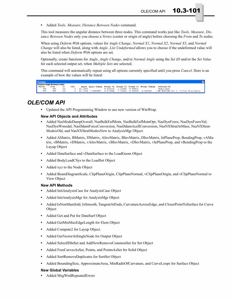
OLE/COM API 10.3-101
• Added Tools, Measure, Distance Between Nodes command.
This tool measures the angular distance between three nodes. This command works just like Tools, Measure, Dis-tance Between Nodes only you choose a Vertex (center or origin of angle) before choosing the From and To nodes.
When using Deform With options, values for Angle Change, Normal X1, Normal X2, Normal X3, and Normal Change will also be listed, along with Angle. List Undeformed allows you to choose if the undeformed value will also be listed when Deform With options are set.
Optionally, create functions for Angle, Angle Change, and/or Normal Angle using the Set ID and/or the Set Value for each selected output set, when Multiple Sets are selected.
This command will automatically repeat using all options currently specified until you press Cancel. Here is an example of how the values will be listed:
OLE/COM API• Updated the API Programming Window to use new version of WinWrap.
New API Objects and Attributes• Added NasModeDampOverall, NasBulkEnfMotn, NasBulkEnfMotnOpt, NasDynFzero, NasDynFzeroVal,
NasDynWmodal, NasDdamForceConversion, NasDdamAcellConversion, NasNXStratAtMass, NasNXStrat-ModexOld, and NasNXStratModexNew to AnalysisMgr Object.
• Added AMatrix, BMatrix, DMatrix, AInvMatrix, BInvMatrix, DInvMatrix, InPlaneProp, BendingProp, vAMa-trix, vBMatrix, vDMatrix, vAInvMatrix, vBInvMatrix, vDInvMatrix, vInPlaneProp, and vBendingProp to the Layup Object
• Added DataSurface and vDataSurface to the LoadGeom Object
• Added BodyLoadCSys to the LoadSet Object
• Added xyz to the Node Object
• Added BeamDiagramScale, ClipPlaneOrigin, ClipPlaneNormal, vClipPlaneOrigin, and vClipPlaneNormal to View Object
New API Methods• Added InitAnalysisCase for AnalysisCase Object
• Added InitAnalysisMgr for AnalysisMgr Object
• Added IsNonManifold, IsSmooth, TangentAtEnds, CurvatureAcrossEdge, and CloserPointToSurface for Curve Object
• Added Get and Put for DataSurf Object
• Added GetMinMaxEdgeLength for Elem Object
• Added Compute2 for Layup Object.
• Added GetVectorAtSingleNode for Output Object
• Added SelectIDInSet and AddNewRemoveCommonSet for Set Object
• Added FreeCurvesAsSet, Points, and PointsAsSet for Solid Object
• Added SortRemoveDuplicates for SortSet Object
• Added BoundingSize, ApproximateArea, MinRadiiOfCurvature, and CurveLoops for Surface Object
New Global Variables• Added MsgWndRepeatedErrors
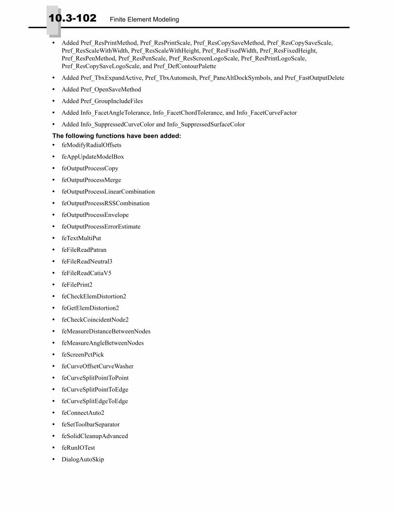
10.3-102 Finite Element Modeling
• Added Pref_ResPrintMethod, Pref_ResPrintScale, Pref_ResCopySaveMethod, Pref_ResCopySaveScale, Pref_ResScaleWithWidth, Pref_ResScaleWithHeight, Pref_ResFixedWidth, Pref_ResFixedHeight, Pref_ResPenMethod, Pref_ResPenScale, Pref_ResScreenLogoScale, Pref_ResPrintLogoScale, Pref_ResCopySaveLogoScale, and Pref_DefContourPalette
• Added Pref_TbxExpandActive, Pref_TbxAutomesh, Pref_PaneAltDockSymbols, and Pref_FastOutputDelete
• Added Pref_OpenSaveMethod
• Added Pref_GroupIncludeFiles
• Added Info_FacetAngleTolerance, Info_FacetChordTolerance, and Info_FacetCurveFactor
• Added Info_SuppressedCurveColor and Info_SuppressedSurfaceColor
The following functions have been added:• feModifyRadialOffsets
• feAppUpdateModelBox
• feOutputProcessCopy
• feOutputProcessMerge
• feOutputProcessLinearCombination
• feOutputProcessRSSCombination
• feOutputProcessEnvelope
• feOutputProcessErrorEstimate
• feTextMultiPut
• feFileReadPatran
• feFileReadNeutral3
• feFileReadCatiaV5
• feFilePrint2
• feCheckElemDistortion2
• feGetElemDistortion2
• feCheckCoincidentNode2
• feMeasureDistanceBetweenNodes
• feMeasureAngleBetweenNodes
• feScreenPctPick
• feCurveOffsetCurveWasher
• feCurveSplitPointToPoint
• feCurveSplitPointToEdge
• feCurveSplitEdgeToEdge
• feConnectAuto2
• feSetToolbarSeparator
• feSolidCleanupAdvanced
• feRunIOTest
• DialogAutoSkip
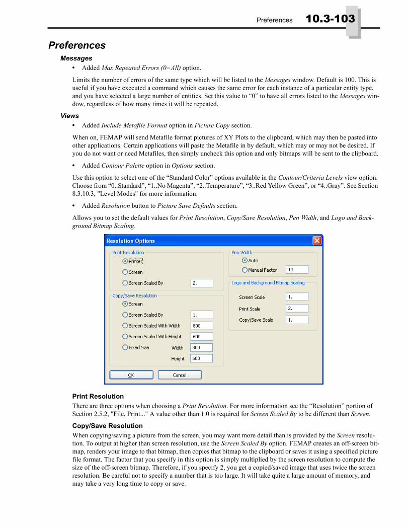
Preferences 10.3-103
PreferencesMessages
• Added Max Repeated Errors (0=All) option.
Limits the number of errors of the same type which will be listed to the Messages window. Default is 100. This is useful if you have executed a command which causes the same error for each instance of a particular entity type, and you have selected a large number of entities. Set this value to “0” to have all errors listed to the Messages win-dow, regardless of how many times it will be repeated.
Views• Added Include Metafile Format option in Picture Copy section.
When on, FEMAP will send Metafile format pictures of XY Plots to the clipboard, which may then be pasted into other applications. Certain applications will paste the Metafile in by default, which may or may not be desired. If you do not want or need Metafiles, then simply uncheck this option and only bitmaps will be sent to the clipboard.
• Added Contour Palette option in Options section.
Use this option to select one of the “Standard Color” options available in the Contour/Criteria Levels view option. Choose from “0..Standard”, “1..No Magenta”, “2..Temperature”, “3..Red Yellow Green”, or “4..Gray”. See Section 8.3.10.3, "Level Modes" for more information.
• Added Resolution button to Picture Save Defaults section.
Allows you to set the default values for Print Resolution, Copy/Save Resolution, Pen Width, and Logo and Back-ground Bitmap Scaling.
Print ResolutionThere are three options when choosing a Print Resolution. For more information see the “Resolution” portion of Section 2.5.2, "File, Print..." A value other than 1.0 is required for Screen Scaled By to be different than Screen.
Copy/Save ResolutionWhen copying/saving a picture from the screen, you may want more detail than is provided by the Screen resolu-tion. To output at higher than screen resolution, use the Screen Scaled By option. FEMAP creates an off-screen bit-map, renders your image to that bitmap, then copies that bitmap to the clipboard or saves it using a specified picture file format. The factor that you specify in this option is simply multiplied by the screen resolution to compute the size of the off-screen bitmap. Therefore, if you specify 2, you get a copied/saved image that uses twice the screen resolution. Be careful not to specify a number that is too large. It will take quite a large amount of memory, and may take a very long time to copy or save.
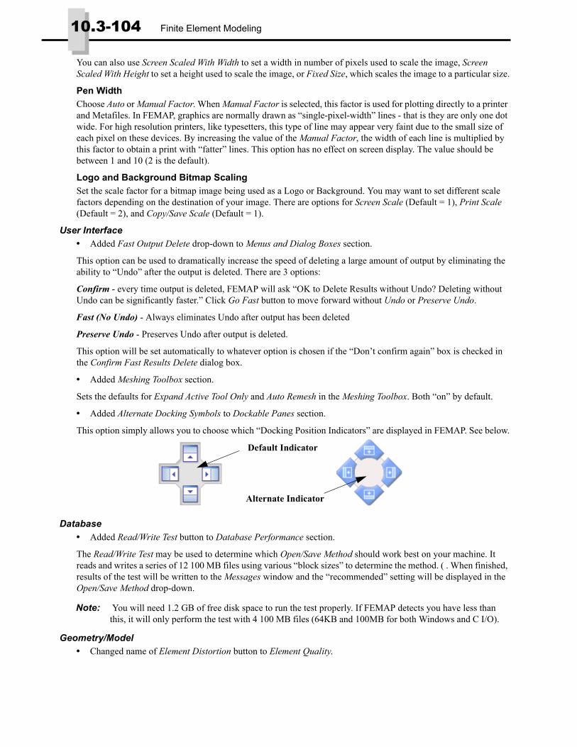
10.3-104 Finite Element Modeling
You can also use Screen Scaled With Width to set a width in number of pixels used to scale the image, Screen Scaled With Height to set a height used to scale the image, or Fixed Size, which scales the image to a particular size.
Pen WidthChoose Auto or Manual Factor. When Manual Factor is selected, this factor is used for plotting directly to a printer and Metafiles. In FEMAP, graphics are normally drawn as “single-pixel-width” lines - that is they are only one dot wide. For high resolution printers, like typesetters, this type of line may appear very faint due to the small size of each pixel on these devices. By increasing the value of the Manual Factor, the width of each line is multiplied by this factor to obtain a print with “fatter” lines. This option has no effect on screen display. The value should be between 1 and 10 (2 is the default).
Logo and Background Bitmap ScalingSet the scale factor for a bitmap image being used as a Logo or Background. You may want to set different scale factors depending on the destination of your image. There are options for Screen Scale (Default = 1), Print Scale (Default = 2), and Copy/Save Scale (Default = 1).
User Interface• Added Fast Output Delete drop-down to Menus and Dialog Boxes section.
This option can be used to dramatically increase the speed of deleting a large amount of output by eliminating the ability to “Undo” after the output is deleted. There are 3 options:
Confirm - every time output is deleted, FEMAP will ask “OK to Delete Results without Undo? Deleting without Undo can be significantly faster.” Click Go Fast button to move forward without Undo or Preserve Undo.
Fast (No Undo) - Always eliminates Undo after output has been deleted
Preserve Undo - Preserves Undo after output is deleted.
This option will be set automatically to whatever option is chosen if the “Don’t confirm again” box is checked in the Confirm Fast Results Delete dialog box.
• Added Meshing Toolbox section.
Sets the defaults for Expand Active Tool Only and Auto Remesh in the Meshing Toolbox. Both “on” by default.
• Added Alternate Docking Symbols to Dockable Panes section.
This option simply allows you to choose which “Docking Position Indicators” are displayed in FEMAP. See below.
Database• Added Read/Write Test button to Database Performance section.
The Read/Write Test may be used to determine which Open/Save Method should work best on your machine. It reads and writes a series of 12 100 MB files using various “block sizes” to determine the method. ( . When finished, results of the test will be written to the Messages window and the “recommended” setting will be displayed in the Open/Save Method drop-down.
Geometry/Model• Changed name of Element Distortion button to Element Quality.
Note: You will need 1.2 GB of free disk space to run the test properly. If FEMAP detects you have less than this, it will only perform the test with 4 100 MB files (64KB and 100MB for both Windows and C I/O).
Default Indicator
Alternate Indicator

Preferences 10.3-105
Interfaces• Added Create Groups from INCLUDE files option to Nastran Solver Write Options section.
This option will automatically create groups based on INCLUDE statements found in imported Nastran input files. Each INCLUDE statement points to a different Nastran input file. The entities found in each unique input file will be placed into a separate group. INCLUDE statements may point to files which also contain INCLUDE statements, creating a “nested” hierarchy. If this is the case, FEMAP will create a “Referenced Group” containing groups (reg-ular or referenced) automatically created from INCLUDE statements. Therefore, it may be possible to have a “ref-erenced group” which references any number of other “referenced groups” or “regular groups”. This is all done to try and keep the hierarchy of the original Nastran input file in place via groups in FEMAP.
• Changed the default for the Direct Output To option in the Nastran Solver Write Options section from “0..Cur-rent Directory” to “1..Model File Directory”.

10.3-106 Finite Element Modeling

What’s New for version 10.1.1 10.3-107
What’s New for version 10.1.1
User InterfaceMenu, Entity Select, Model Info tree, Data Table, Graphics
Menu• Added File, Picture, Copy Desktop command. Works much like File, Picture, Save Desktop, except it copies a
picture of the entire FEMAP GUI to the clipboard instead of saving it to a file.
• Added File, Picture, Copy Layout and File, Picture, Save Layout commands. These commands work much like File, Picture, Copy Desktop and File, Picture, Save Desktop, except they only copy to the clipboard or save to a file the contents of the “Graphics Area” instead of the entire GUI.
• Added Delete, Model, Mesh on Nodes command. Works exactly like Delete, Model, Mesh except nodes are selected instead of elements.
Entity Select• Added the ability to quickly access “Polygon picking” without choosing “Polygon” from the “Pick” menu in
the Entity Selection dialog box. Simply hold down both the Shift and Ctrl keys at once and press the left mouse button to specify the first point of the selection polygon, then click additional points on the screen until the appropriate area is within the polygon.
• Added “Filter” and “Clear All Filters” buttons and corresponding text field to the “Select One or More...” dia-log boxes displayed when the Select From List button is pressed in the Entity Selection dialog box. Once text is entered into the text field click the Filter icon button to reduce the list to just those entries that contain the text you specified. You can now enter additional text, then press Filter icon button again to further reduce the list. Press Clear All Filters icon button to return to the full list and start again.
• Added “Color” option to the “Pick” menu of the Entity Selection dialog box. This option allows you to select a color from the Color Palette, then adds all entities of the current type which are also the selected color to the selection list. Options also exist to Match Color, Match Pattern/Transparency, and Match Line Style options which may turned on/off to either broaden or narrow the selection criteria. By default, all Options are on.

10.3-108 Finite Element Modeling
• Added “Property/Material Value” option to the “Pick” menu of the Entity Selection dialog box. This option allows you to choose entities in the model with values Equal to a specific material/property value (i.e., Plane Element Thickness, Young’s Modulus, BEAM End A Area etc.) or entities which have values within a range (Above or Below a single value; Between or Outside two values) for a particular material/property entry.
• Improved “Copy as List” option on the “Pick” menu of the Entity Selection dialog box. Using this function on “Large” models containing several million nodes has gone from taking hours to taking seconds.
• Added “Filter” and “Clear All Filters” buttons and corresponding text field to all “Select ‘single entity’ from list” dialog boxes. An example of a command that would display such a dialog box would be Modify, Update Elements, Property ID, which displays “Select Property for Update”.
• Added graphical picking of Solids from the Solid Manager dialog box. Also, the displayed Loads Set, Con-straint Set, Group (only when single group displayed), or View can be graphically chosen from the screen and then become highlighted in the appropriate Manager dialog box.
Model Info tree• Added “Auto Create Definition” to context-sensitive menu for “Other Loads”. Allows you to highlight any
number of loads and will automatically create new load definitions based on load type, load values, and addi-tional load information (i.e., loaded face of an element). A new definition will be created for loads of the same type which have different values and/or different additional load information, which differs from the Create Definition command.
• Added ability to hold down Alt key and left click the “expand/collapse” toggle to expand/collapse all of the “sub-branches” under the highlighted branch. Also, pressing the right arrow key while holding down the Alt key will “expand” all sub-branches, while pressing the left arrow with Alt will “collapse” all sub-branches.
Data Table• Added “Select All” command on context-sensitive menu for the Data Table. Selects all rows currently in the
Data Table regardless of which rows are currently highlighted.
Graphics• Improved performance of undo/redo of surface facets.

Geometry 10.3-109
Geometry• Added 3 “Align” options to the Geometry, Curve - From Surface, Pad command
The orientation of the “pad” can specified 3 separate ways. Auto Align will simple use a circular curve’s existing points and extend out from them. Vector Align allows you to specify an orientation vector so the pad can be posi-tioned in a certain orientation. Finally, Tangent Align will prompt you to select an additional curve and then create a pad which has an outer edge aligned tangent to the selected curve.
Meshing• Added automatically assigning corners to surfaces with more than 4 corners when using the “Mapped - Four
Corner” approach of the Mesh, Mesh Control, Approach on Surface command.
If you do not select any “corners”, FEMAP will attempt to choose appropriate “corners” on certain types of sur-faces. This includes surfaces with more than four points.
Example surfaces where “corners” likely do not need to be selected to achieve mapped mesh:
• Added “Radial Offset Around Vector” option to Modify, Update Elements, Line Element Offsets command.
• Improved performance of midside node attachment significantly, especially on models with a large number of geometric entities (Surfaces, Curves. Points). This capability is used when creating new mesh on a solid, as well as when using the Modify, Associativity, Automatic command.
Pads With “Auto Align” Pads With “Vector Align”(aligned to displayed Vector)
Pads With “Tangent Align”(Aligned using closest curves)
Surfaces with all points shown Automatically selected “mesh corners” shown withresulting mesh

10.3-110 Finite Element Modeling
Elements• Added “New Node At Center” method to Independent (Reference) section of Define RIGID Element dialog
box. When this method is used, FEMAP will automatically create a node at “center” of all the selected Depen-dent (Nodes to Average) nodes, much like the “Spider” API command.
• Added “Convert” button to Define RIGID Element dialog box. This button is used to convert a rigid element to an interpolation element and vice versa. When converting from rigid element to interpolation, FEMAP will ask “OK to Convert only Translational Degrees of Freedom?”.
• Added “Distance Weighting” option to the Update Interpolation Element dialog box displayed after clicking the “Update” button in Define RIGID Element dialog box. This option will create different interpolation factors for highlighted Nodes to Average based on their distance from the Reference node. Multiple nodes must be highlighted in the list for this option to have any effect.
Materials• Added support for Sussman-Bathe hyperelastic material to Other Types for solution 601 in NX Nastran
• Added support for Shape Memory Alloy material to Other Types for solution 601 in NX Nastran
Layups• Added ability to create PCOMPG instead of PCOMP entries for Nastran by specifying a Global Ply for every
Ply in a Layup. If even 1 ply does not have a Globally Ply assigned, the PCOMP will be written instead.

Loads and Constraints 10.3-111
The following Layup would be written as a PCOMPG:
• Added “Ok to Update Material and Thickness of Global Ply # in all Layups?” question to Edit Ply capability in the Global Ply Definition dialog box.
Loads and Constraints• Added “Bearing Force” Load type to “Model, Load, On Surface” command.
When creating a Bearing Force, enter a Magnitude, Load Angle (specifies the area in which the “bearing” is in con-tact, entered in degrees. 180 is the default), and Phase (if needed), then specify a vector to represent the direction of the load. Additionally, there is an option to have the Bearing Force be Normal to Surface (“on” by default), which will apply the loads radially to cylindrical surfaces. Also, the load may be a Traction Load (“off “by default), which will essentially have the load “pull” on a surface instead of “push”.
Bearing Force on single
Bearing Force on multiplesurfaces with “Total Load” and “Normal to Surface” options “On”
Bearing Force on multiplesurfaces with “Total Load”, “Normal to Surface”, and “Traction Load” options “On”
surface with “Normal toSurface” option “On”
Bearing Force on singlesurface with “Normal toSurface” option “Off”
Vector used to definebearing forces on this
Vector used to definebearing forces on this
line
line
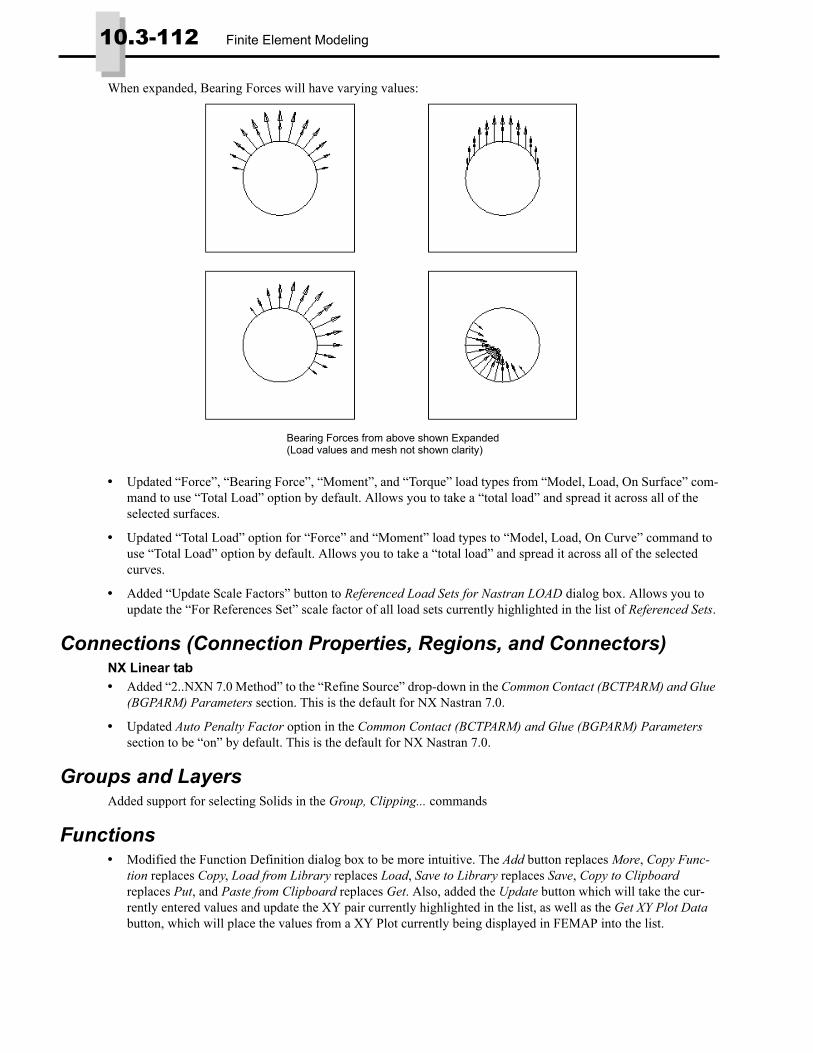
10.3-112 Finite Element Modeling
When expanded, Bearing Forces will have varying values:
• Updated “Force”, “Bearing Force”, “Moment”, and “Torque” load types from “Model, Load, On Surface” com-mand to use “Total Load” option by default. Allows you to take a “total load” and spread it across all of the selected surfaces.
• Updated “Total Load” option for “Force” and “Moment” load types to “Model, Load, On Curve” command to use “Total Load” option by default. Allows you to take a “total load” and spread it across all of the selected curves.
• Added “Update Scale Factors” button to Referenced Load Sets for Nastran LOAD dialog box. Allows you to update the “For References Set” scale factor of all load sets currently highlighted in the list of Referenced Sets.
Connections (Connection Properties, Regions, and Connectors)NX Linear tab• Added “2..NXN 7.0 Method” to the “Refine Source” drop-down in the Common Contact (BCTPARM) and Glue
(BGPARM) Parameters section. This is the default for NX Nastran 7.0.
• Updated Auto Penalty Factor option in the Common Contact (BCTPARM) and Glue (BGPARM) Parameters section to be “on” by default. This is the default for NX Nastran 7.0.
Groups and LayersAdded support for selecting Solids in the Group, Clipping... commands
Functions• Modified the Function Definition dialog box to be more intuitive. The Add button replaces More, Copy Func-
tion replaces Copy, Load from Library replaces Load, Save to Library replaces Save, Copy to Clipboard replaces Put, and Paste from Clipboard replaces Get. Also, added the Update button which will take the cur-rently entered values and update the XY pair currently highlighted in the list, as well as the Get XY Plot Data button, which will place the values from a XY Plot currently being displayed in FEMAP into the list.
Bearing Forces from above shown Expanded(Load values and mesh not shown clarity)
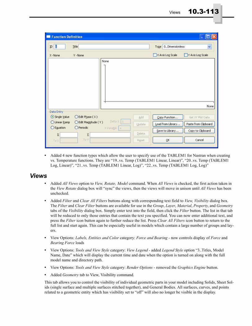
Views 10.3-113
• Added 4 new function types which allow the user to specify use of the TABLEM1 for Nastran when creating vs. Temperature functions. They are “19..vs. Temp (TABLEM1 Linear, Linear)”, “20..vs. Temp (TABLEM1 Log, Linear)”, “21..vs. Temp (TABLEM1 Linear, Log)”, “22..vs. Temp (TABLEM1 Log, Log)”
Views• Added All Views option to View, Rotate, Model command. When All Views is checked, the first action taken in
the View Rotate dialog box will “sync” the views, then the views will move in unison until All Views has been unchecked.
• Added Filter and Clear All Filters buttons along with corresponding text field to View, Visibility dialog box. The Filter and Clear Filter buttons are available for use in the Group, Layer, Material, Property, and Geometry tabs of the Visibility dialog box. Simply enter text into the field, then click the Filter button. The list in that tab will be reduced to only those entries that contain the text you specified. You can now enter additional text, and press the Filter icon button again to further reduce the list. Press Clear All Filters icon button to return to the full list and start again. This can be especially useful in models which contain a large number of groups and lay-ers.
• View Options: Labels, Entities and Color category: Force and Bearing - now controls display of Force and Bearing Force loads
• View Options: Tools and View Style category: View Legend - added Legend Style option “3..Titles, Model Name, Date” which will display the current time and date when the option is turned on along with the full model name and directory path.
• View Options: Tools and View Style category: Render Options - removed the Graphics Engine button.
• Added Geometry tab to View, Visibility command.
This tab allows you to control the visibility of individual geometric parts in your model including Solids, Sheet Sol-ids (single surface and multiple surfaces stitched together), and General Bodies. All surfaces, curves, and points related to a geometric entity which has visibility set to “off” will also no longer be visible in the display.
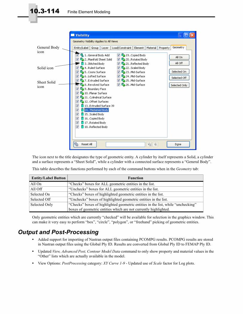
10.3-114 Finite Element Modeling
The icon next to the title designates the type of geometric entity. A cylinder by itself represents a Solid, a cylinder and a surface represents a “Sheet Solid”, while a cylinder with a connected surface represents a “General Body”.
This table describes the functions performed by each of the command buttons when in the Geometry tab:
Only geometric entities which are currently “checked” will be available for selection in the graphics window. This can make it very easy to perform “box”, “circle”, “polygon”, or “freehand” picking of geometric entities.
Output and Post-Processing• Added support for importing of Nastran output files containing PCOMPG results. PCOMPG results are stored
in Nastran output files using the Global Ply ID. Results are converted from Global Ply ID to FEMAP Ply ID.
• Updated View, Advanced Post, Contour Model Data command to only show property and material values in the “Other” lists which are actually available in the model.
• View Options: PostProcessing category: XY Curve 1-9 - Updated use of Scale factor for Log plots.
Entity/Label Button FunctionAll On “Checks” boxes for ALL geometric entities in the list.All Off “Unchecks” boxes for ALL geometric entities in the list.Selected On “Checks” boxes of highlighted geometric entities in the list.Selected Off “Unchecks” boxes of highlighted geometric entities in the list.Selected Only “Checks” boxes of highlighted geometric entities in the list, while “unchecking”
boxes of geometric entities which are not currently highlighted.
General Bodyicon
Solid icon
Sheet Solid icon

Geometry Interfaces 10.3-115
Geometry InterfacesThe following FEMAP interfaces have been updated to support newer geometry formats:
• Added support to optionally read or skip blanked/invisible/hidden parts when importing NX 6 assemblies
• Restored support for ACIS versions 7, 8, and 9, which had been removed in a previous version.
For details, see “Geometry Interfaces” in the FEMAP User Guide.
Analysis Program InterfacesSeveral of the analysis program interfaces have been improved. These changes include:
• Analysis Set Manager Enhancements
• FEMAP Neutral File Interface
• NX Nastran Interface
• Nastran Interfaces (NX and MSC/MD)
• MSC/MD Nastran Interface
• ABAQUS Interface
Analysis Set Manager EnhancementsFor details, see “Analysis Program Interfaces” in the FEMAP User Guide.
• Improved performance of the Preview window significantly.
• Added ability to hold down Alt key and left click the “expand/collapse” toggle to expand/collapse all of the “sub-branches” under the highlighted branch. Also, pressing the right arrow key while holding down the Alt key will “expand” all sub-branches, while pressing the left arrow with Alt will “collapse” all sub-branches.
• Enhanced Analysis Multiple capability for MSC Nastran to perform as expected.
FEMAP Neutral File Interface• Updated Neutral Write to use the proper versions of ACIS and Parasolid when exporting neutral files for older
version of FEMAP.
NX Nastran Interface• Added Support for BCTADD and BGADD entries for version 7.0
• Updated XDB import to only allow reading of regular stress or nonlinear stress, not both.
• Added support for Sussman-Bathe hyperelastic material
• Added support for Shape Memory Alloy material
A number of bugs were corrected
For details, see “Analysis Program Interfaces” in the FEMAP User Guide.
Nastran Interfaces (NX and MSC/MD)• Added support for PCOMPG entry
FEMAP Interface Latest Supported VersionParasolid Parasolid 22.0Solid Edge Solid Edge with Synchronous Technology 2NX NX 7Pro/Engineer Wildfire 4ACIS ACIS 20CATIA V5 V5 release 19SolidWorks SolidWorks 2009

10.3-116 Finite Element Modeling
• Added support to read the QVOL, CONV, PCONV, QHBDY, QVECT, QBDY1, CHBDYG, VIEW, VIEW3D, RADM, RADMT, RADCAV, and RADSET entries
• Added support to read and write PARAM,SIGMA and PARAM,TABS
• Added support to write TABLEM1 entries when creating vs. Temperature functions using specific function types in FEMAP.
• Added ability to Skip NLPARM in the Nonlinear Control Options dialog box for the Master and all Subcases when creating an analysis set for a nonlinear analysis.
A number of bugs were corrected
For details, see “Analysis Program Interfaces” in the FEMAP User Guide.
MSC/MD Nastran InterfaceA number of bugs were corrected.
For details, see “Analysis Program Interfaces” in the FEMAP User Guide.
NEi Nastran InterfaceA number of bugs were corrected.
For details, see “Analysis Program Interfaces” in the FEMAP User Guide.
ABAQUS InterfaceA number of bugs were corrected.
For details, see “Analysis Program Interfaces” in the FEMAP User Guide.
OLE/COM API• For functions that take input arguments that are Arrays/Variants, you can now pass a single value/constant
directly if the entire array is supposed to be filled with the same value.
• Disabled Undo after calling feFileRebuild, feFileSave, feFileSaveAs, and feFileSaveAll from the API.
• Converted UserData to a non-Entity-based object. Implemented numerous methods that are identical in call to Entity-based objects, but work properly with UserData
New API Objects and Attributes• Added Length to Element object
New API Methods• Added AddAllTitle, AddAllColor, and AddMidsideNodes to Set object
• Added ComputeStdShape and ComputeGeneralShape for Property object
• Added CountLoads and IsTotalLoad for LoadDefinition object
• Added Add to LoadMesh object
• Added Add to BCNode object
• Added Preview to AnalysisMgr object
• Added HasFullGlobalPly for Layup object
New Global Variables• Added Pref_PictureCopyTextForXY
• Added Pref_PictureFormat, Pref_AnimationFormat, Pref_GIFColorOpt, Pref_GIFAnimationDelay, and Pref_GIFFrameSeries
• Added Pref_NasQstOn, Pref_NasQstVal, and Pref_DeleteRdScratchLdSets
• Added Pref_CustomToolsPath
Preferences 10.3-117
The following functions have been added:• feAppMessageStartListing
• feAppMessageEndListing
• feFilePictureSave2
• feFilePictureCopy2
• feFormatReal
• feTruncateReal
• feModifyRadialOffsets
• feDeleteMesh
PreferencesViews• Added Include Text for XY Plots option in Picture Copy section.
When on, which is the default, the XY values representing the data points in the XY plot will be sent as a table of XY values to the clipboard. When off, this table will not be sent to the clipboard.
• Added Picture Save Defaults section.
These options control set defaults file format when using the File, Picture, Save; File, Picture, Save Layout; and File, Picture, Save Desktop commands.
Picture
Sets the default file format when using any of the File, Picture commands, while the display is NOT animating. Choices are Bitmap (*.BMP), JPEG (*.JPG), GIF(*.GIF), PNG(*.PNG), or TIFF (*.TIF).
Animation
Sets default file format when using the File, Picture, Copy command, only when the display is animating. Choices are Bitmap (*.BMP), Bitmap Series (*.BMP), Video for Windows (*.AVI), or Animated GIF (*.GIF).
GIF Options button
Sets default options when saving a GIF or Animated GIF file. For GIF files, choose from Network, Octree, and Color Diffusion (Dither). In addition, the Frame Delay may be set for animated GIFs (milliseconds) and an option exists to Save GIF Frame Series. Depending on your machine and other applications where you might be placing saved pictures, one of these formats may produce a better image than the other two or similar image quality using a smaller file size.
User Interface• Added Captions Always on Top option to Dockable Panes section.
This option will force the Title Bar of any “docked” dockable pane to always be on the top of the pane, regardless of where the pane is currently docked. By default, dockable panes which are docked on the top or bottom of the graphics area will have the title bar displayed on the left side of the pane to use less space vertically.
Interfaces• Added Auto Answer Post Questions button.
Pressing this button will display a dialog box which will allow you to toggle “Auto Answer” check boxes for a variety of questions which may appear in dialog boxes during import of Nastran results from .f06 file. One addi-tional General Question may also be “auto-answered” with regard to reading Nonlinear Stresses and Strains from the .f06 and .op2 files.
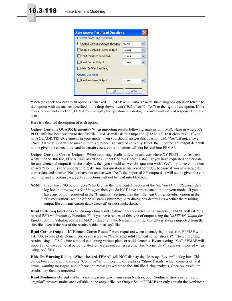
10.3-118 Finite Element Modeling
When the check box next to an option is “checked”, FEMAP will “Auto Answer” the dialog box question related to that option with the answer specified in the drop-down menu (“0..No” or “1..Yes”) to the right of the option. If the check box is “not checked”, FEMAP will display the question in a dialog box and await manual response from the user.
Here is a detailed description of each option:
Output Contains QUADR Elements - When importing results following analysis with MSC Nastran where XY PLOT info has been written to the .f06 file, FEMAP will ask “Is Output on QUADR/TRIAR elements?”. If you have QUADR/TRIAR elements in your model, then you should answer this question with “Yes”, if not, answer “No”. It is very important to make sure this question is answered correctly. If not, the imported XY output data will not be given the correct title, and in certain cases, entire functions will not be read into FEMAP.
Output Contains Corner Output - When importing results following analysis where XY PLOT info has been written to the .f06 file, FEMAP will ask “Does Output Contain Corner Data?”. If you have requested corner data for any elemental output from the analysis, then you should answer this question with “Yes”, if you have not, then answer “No”. It is very important to make sure this question is answered correctly, because if you have requested corner data and answer “No”, or have not and answer “Yes”, the imported XY output data will not be given the cor-rect title, and in certain cases, entire functions will not be read into FEMAP..
Read PSD/Freq functions - When importing results following Random Response analysis, FEMAP will ask “OK to read PSD vs. Frequency Functions?”. If you have requested this type of output using the NASTRAN Output for Random Analysis dialog box in FEMAP or directly in the Nastran input file, this data is always imported from the .f06 file, even if the rest of the results reside in an .op2 file.
Read Corner Output - If “Element Corner Results” were requested when an analysis job was run, FEMAP will ask “OK to read plate element corner stresses?” or “OK to read solid element corner stresses?” when importing results using a .f06 file into a model containing various plane or solid elements. By answering “Yes”, FEMAP will import all of the additional output related to the element corner results. This “corner data” is always imported when using .op2 files.
Hide f06 Warning Dialog - When checked, FEMAP will NOT display the “Message Review” dialog box. This dialog box allows you to simply “Continue” with importing of results or “Show Details” which consists of fatal errors, warning messages, and information messages written to the .f06 file during analysis. Once reviewed, the results may then be imported.
Read Nonlinear Output - When a nonlinear analysis is run using Nastran, both Nonlinear stresses/strains and “regular” stresses/strains are available in the output file. An Output Set in FEMAP can only contain the Nonlinear
Note: If you have NO output types “checked” in the “Elemental” section of the Nastran Output Requests dia-log box in the Analysis Set Manager, then you do NOT have corner data output in your model. If you have any output requested in the “Elemental” section, then the “Element Corner Results” option in the “Customization” section of the Nastran Output Requests dialog box determines whether the resulting output file contains corner data (checked) or not (unchecked).

Preferences 10.3-119
OR the “Regular” stresses/strains, not both. Checking this option will always read in the Nonlinear stresses/strains from the output file of a nonlinear analysis. If this option is not checked, which is the default, FEMAP will bring up a dialog box during the import of results which allows you to choose which stresses/strains to read (Yes = Nonlin-ear, No = “Regular”).
• Added Delete Read Synthetic Load Sets option.
When importing a Nastran input file, several additional load sets are sometimes created to facilitate combinations of structural, thermal, and dynamic loads. FEMAP allows different types of loads to be in a single load set, so often these additional load sets are not required after they have been assembled. When this option is “on”, FEMAP will simply delete these component load sets, as they are no longer needed.

10.3-120 Finite Element Modeling
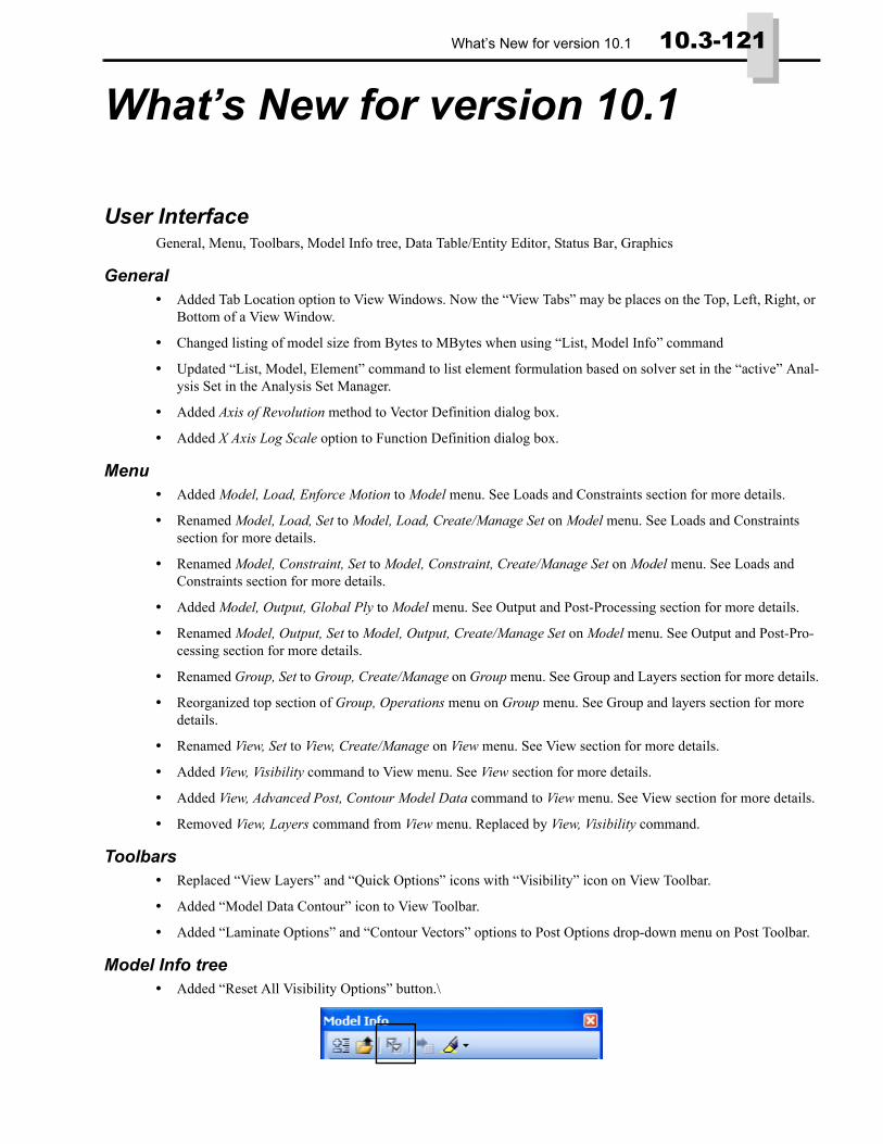
What’s New for version 10.1 10.3-121
What’s New for version 10.1
User InterfaceGeneral, Menu, Toolbars, Model Info tree, Data Table/Entity Editor, Status Bar, Graphics
General• Added Tab Location option to View Windows. Now the “View Tabs” may be places on the Top, Left, Right, or
Bottom of a View Window.
• Changed listing of model size from Bytes to MBytes when using “List, Model Info” command
• Updated “List, Model, Element” command to list element formulation based on solver set in the “active” Anal-ysis Set in the Analysis Set Manager.
• Added Axis of Revolution method to Vector Definition dialog box.
• Added X Axis Log Scale option to Function Definition dialog box.
Menu• Added Model, Load, Enforce Motion to Model menu. See Loads and Constraints section for more details.
• Renamed Model, Load, Set to Model, Load, Create/Manage Set on Model menu. See Loads and Constraints section for more details.
• Renamed Model, Constraint, Set to Model, Constraint, Create/Manage Set on Model menu. See Loads and Constraints section for more details.
• Added Model, Output, Global Ply to Model menu. See Output and Post-Processing section for more details.
• Renamed Model, Output, Set to Model, Output, Create/Manage Set on Model menu. See Output and Post-Pro-cessing section for more details.
• Renamed Group, Set to Group, Create/Manage on Group menu. See Group and Layers section for more details.
• Reorganized top section of Group, Operations menu on Group menu. See Group and layers section for more details.
• Renamed View, Set to View, Create/Manage on View menu. See View section for more details.
• Added View, Visibility command to View menu. See View section for more details.
• Added View, Advanced Post, Contour Model Data command to View menu. See View section for more details.
• Removed View, Layers command from View menu. Replaced by View, Visibility command.
Toolbars• Replaced “View Layers” and “Quick Options” icons with “Visibility” icon on View Toolbar.
• Added “Model Data Contour” icon to View Toolbar.
• Added “Laminate Options” and “Contour Vectors” options to Post Options drop-down menu on Post Toolbar.
Model Info tree• Added “Reset All Visibility Options” button.\
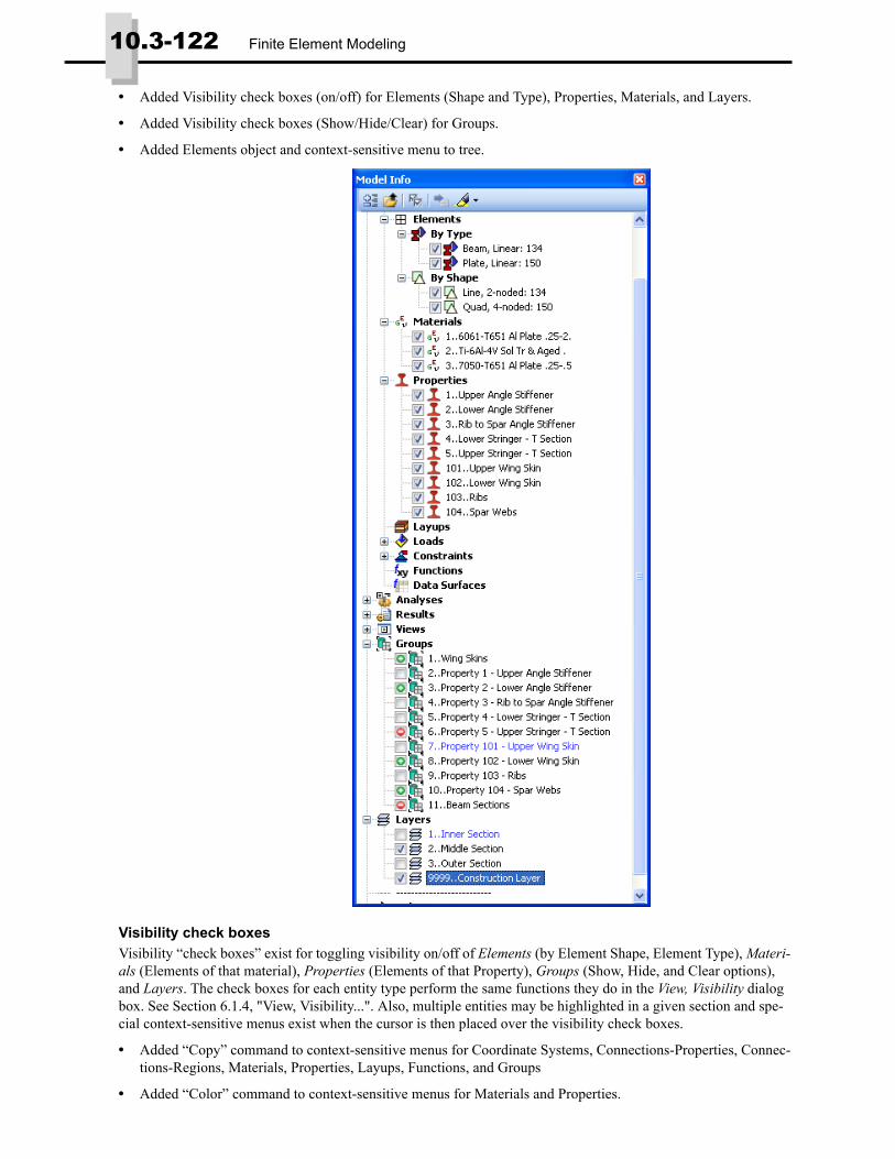
10.3-122 Finite Element Modeling
• Added Visibility check boxes (on/off) for Elements (Shape and Type), Properties, Materials, and Layers.
• Added Visibility check boxes (Show/Hide/Clear) for Groups.
• Added Elements object and context-sensitive menu to tree.
Visibility check boxesVisibility “check boxes” exist for toggling visibility on/off of Elements (by Element Shape, Element Type), Materi-als (Elements of that material), Properties (Elements of that Property), Groups (Show, Hide, and Clear options), and Layers. The check boxes for each entity type perform the same functions they do in the View, Visibility dialog box. See Section 6.1.4, "View, Visibility...". Also, multiple entities may be highlighted in a given section and spe-cial context-sensitive menus exist when the cursor is then placed over the visibility check boxes.
• Added “Copy” command to context-sensitive menus for Coordinate Systems, Connections-Properties, Connec-tions-Regions, Materials, Properties, Layups, Functions, and Groups
• Added “Color” command to context-sensitive menus for Materials and Properties.

Data Table/Entity Editor 10.3-123
• Added “Layer” command to context-sensitive menus for Materials and Properties.
• Added “Global Ply” command to Layups context-sensitive menu.
• Added “Referenced Sets” command to context-sensitive menus for Loads and Constraints.
• Added “Edit Where Applied” command to context-sensitive menus for Load Definitions and Constraint Defini-tions.
• Changed “Edit” command to “Edit Load” on Load Definition context-sensitive menu.
• Changed “Edit” command to “Edit Constraint” on Constraint Definition context-sensitive menu.
• Added “Show Constrained Entities” command to Constraints context-sensitive menu.
• Added “Referenced Groups” command to Groups context-sensitive menu.
• Changed “View Active” command to “Show Active Group” and added “Show Full Model” and “Show Multi-ple Groups” to Groups context-sensitive menu.
• Changed “Show All Layers” to “View All Layers” and “Show Visible Layers Only” to “View Visible Layers Only” on Layers context-sensitive menu.
• Removed “Make Visible”, “Make Hidden”, and “Manage” commands from Layers context-sensitive menu. No longer needed due to Visibility check boxes.
Data Table/Entity Editor• Added “Memb-Bend Coupling” fields for plate elements.
• Added support for “Nastran LOAD Combination Sets” and “Nastran SPCADD/MPCADD Combination Sets”
Status Bar• Changed “Set” to “Create/Manage (Set)” for Load Sets, Constraint Sets, Groups, and Output Sets
• Changed “View Active” to “Show Active” for Groups and added “Show Full Model” and “Show Multiple” options
GraphicsFacets are now stored in memory instead of with the model file. When model is opened, it will be facetted. This is beneficial as model files containing a large amount of geometry will be smaller.
Geometry• Implemented the Solid Manager which is used to activate, update, or make no solids active in the model.
• Modified Geometry, Curve - From Surface, Pad command. Entering an Pad Size Factor of 1.0 will extend curves out using the radius of the chosen circular curves, while entering a value of 1.5 would offset the curves 1.5*the radius of the chosen circular curves in all directions.
Meshing• Added “Use Reference Point” option to Mesh, Mesh Control, Attributes Along Curve
Elements• Added Update Button to Define RIGID Element dialog box. Allows you to update the Interpolation Factor and
DOFs on any number of highlighted nodes in the Nodes to Average section when using the Interpolation option.
Layups• Updated Global Ply Definition dialog box for Layups
Global Ply ID (optional):This option can be used to save a particular ply of one layup for use in other layups in your model.
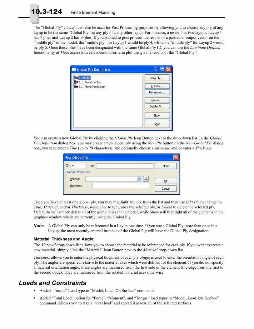
10.3-124 Finite Element Modeling
The “Global Ply” concept can also be used for Post Processing purposes by allowing you to choose any ply of any layup to be the same “Global Ply” as any ply of a any other layup. For instance, a model has two layups, Layup 1 has 7 plies and Layup 2 has 9 plies. If you wanted to post process the results of a particular output vector on the “middle ply” of the model, the “middle ply” for Layup 1 would be ply 4, while the “middle ply” for Layup 2 would be ply 5. Once these plies have been designated with the same Global Ply ID, you can use the Laminate Options functionality of View, Select to create a contour/criteria plot using a the results of the “Global Ply”.
You can create a new Global Ply by clicking the Global Ply Icon Button next to the drop down list. In the Global Ply Definition dialog box, you may create a new global ply using the New Ply button. In the New Global Ply dialog box, you may enter a Title (up to 79 characters), and optionally choose a Material, and/or enter a Thickness.
Once you have at least one global ply, you may highlight any ply from the list and then use Edit Ply to change the Title, Material, and/or Thickness, Renumber to renumber the selected ply, or Delete to delete the selected ply, Delete All will simply delete all of the global plies in the model, while Show will highlight all of the elements in the graphics window which are currently using the Global Ply.
Material, Thickness and Angle:The Material drop-down list allows you to choose the material to be referenced for each ply. If you want to create a new material, simply click the “Material” Icon Button next to the Material drop-down list.
Thickness allows you to enter the physical thickness of each ply. Angle is used to enter the orientation angle of each ply. The angles are specified relative to the material axes which were defined for the element. If you did not specify a material orientation angle, these angles are measured from the first side of the element (the edge from the first to the second node). They are measured from the rotated material axes otherwise.
Loads and Constraints• Added “Torque” Load type to “Model, Load, On Surface” command.
• Added “Total Load” option for “Force”, “Moment”, and “Torque” load types to “Model, Load, On Surface” command. Allows you to take a “total load” and spread it across all of the selected surfaces.
Note: A Global Ply can only be referenced in a Layup one time. If you use a Global Ply more than once in a Layup, the most recently entered instance of the Global Ply will have the Global Ply designation.

Loads and Constraints 10.3-125
• Added “Total Load” option for “Force” and “Moment” load types to “Model, Load, On Curve” command. Allows you to take a “total load” and spread it across all of the selected curves.
• Implemented the Load Set Manager for creation, management, and activation of Load Sets
• Added option to create a Load “Set Type” option which allows you to create a Nastran LOAD Combination and use Referenced Load Sets
Load Set Type
You may choose a Set Type for the new load set. A Standard load set is any combination of Load Definitions, Body Loads, and Other Loads used to define the loading conditions for that load set.
A Nastran LOAD Combination is a special type of load set which is a combination of “referenced” Standard load sets in the model. When used, all of the selected Standard load sets referenced by a Nastran LOAD Combination Set are written to the Nastran input file and combined by Nastran via a LOAD entry also written to the input file.
Note: Only Forces, Moments, Pressures, loads on Scalar points (SPOINTS), Rotational Velocity Body Loads, and Gravity Loads may be combined using the LOAD entry. Also, Nastran LOAD Combinations in FEMAP are only used when performing a Static Analysis.
Create new load sets
Renumber highlighted
Update the title of anexisting load set
Load Set
Delete highlightedLoad Set
Delete all Load Sets
Copy highlightedLoad Set
Define “Nastran LOAD
Deactivate All LoadSets
Combination Set”
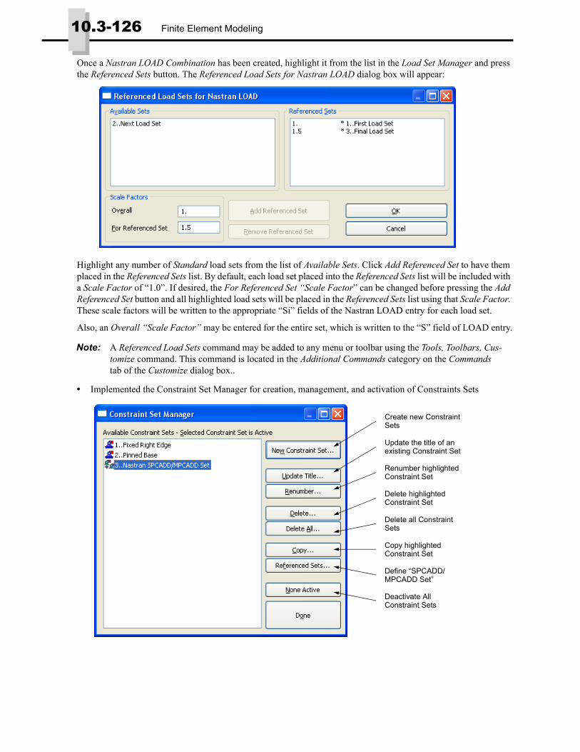
10.3-126 Finite Element Modeling
Once a Nastran LOAD Combination has been created, highlight it from the list in the Load Set Manager and press the Referenced Sets button. The Referenced Load Sets for Nastran LOAD dialog box will appear:
Highlight any number of Standard load sets from the list of Available Sets. Click Add Referenced Set to have them placed in the Referenced Sets list. By default, each load set placed into the Referenced Sets list will be included with a Scale Factor of “1.0”. If desired, the For Referenced Set “Scale Factor” can be changed before pressing the Add Referenced Set button and all highlighted load sets will be placed in the Referenced Sets list using that Scale Factor. These scale factors will be written to the appropriate “Si” fields of the Nastran LOAD entry for each load set.
Also, an Overall “Scale Factor” may be entered for the entire set, which is written to the “S” field of LOAD entry.
• Implemented the Constraint Set Manager for creation, management, and activation of Constraints Sets
Note: A Referenced Load Sets command may be added to any menu or toolbar using the Tools, Toolbars, Cus-tomize command. This command is located in the Additional Commands category on the Commands tab of the Customize dialog box..
Create new Constraint
Renumber highlighted
Update the title of anexisting Constraint Set
Constraint Set
Delete highlightedConstraint Set
Delete all Constraint
Copy highlightedConstraint Set
Define “SPCADD/MPCADD Set”
Deactivate AllConstraint Sets
Sets
Sets

Connections (Connection Properties, Regions, and Connectors) 10.3-127
• Added option to create a Load Set which represents a Nastran SPCADD/MPCDD Combination and use Refer-enced Constraint Sets
You may choose a Set Type for the new constraint set. A Standard constraint set is any combination of Constraint Definitions and Other Loads used to define the boundary conditions for that constraint set.
A Nastran SPCADD/MPCADD Combination is a special type of constraint set which “references” any number of existing Standard constraint sets in the model. When used, all of the selected Standard constraint sets referenced by a particular Nastran SPCADD/MPCADD Combination are written to the Nastran input file and combined by Nas-tran via a SPCADD entry when dealing with normal constraints or a MPCADD when dealing with constraint equa-tions.
Once a Nastran SPCADD/MPCADD Combination Set has been created, highlight it from the list in the Constraint Set Manager and press the Referenced Sets button. The Referenced Constraint Sets for Nastran SPCADD/MPCADD dialog box will appear:
Highlight any number of Standard constraint sets from the list of Available Sets. Click Add Referenced Set to have them placed in the Referenced Sets list.
Connections (Connection Properties, Regions, and Connectors)• Added “Reverse” button to Connection Regions to switch “positive” to “negative” and vice versa for surfaces
and “Face 1” to “Face 2” and vice versa for shell elements.
NX Linear tab• Added Adaptive Stiffness and Penetration Factor to the Contact Property (BCTPARM) section. Create the
PENAPAPT and PENETFAC fields on the BCTPARM entry.
• Added Glue Type and Glue Factor to the Common Contact (BCTPARM) and Glue (BGPARM) Parameters sec-tion. Create the GLUETYPE and PENGLUE fields on the BGPARM entry.
• Added Auto Penalty Factor to the Common Contact (BCTPARM) and Glue (BGPARM) Parameters section. Creates the PENAUTO field on the BCTPARM entry.
Note: A Referenced Constraint Sets command may be added to any menu or toolbar using the Tools, Toolbars, Customize command. This command is located in the Additional Commands category on the Com-mands tab of the Customize dialog box..

10.3-128 Finite Element Modeling
• Modified Penalty Factor Units in the Common Contact (BCTPARM) and Glue (BGPARM) Parameters section to have different options depending on what option is set for Connect Type.
NEiNastran tab• Added 10..Offset Welded Contact option to Penetration Type drop-down list.
Groups and Layers• Implemented the Group Manager for creation, management, and activation of Groups
• Added ability to create “Referenced Groups”
The concept of Referenced Groups allows an existing group to “reference” other existing groups in your model (essentially, create a “Group of Groups”). A group which “references” other groups may also contain any number
Group containingReferenced Groupsicon
Create new Group
Renumber highlighted
Update the title of anexisting Group
Constraint Set
Delete highlightedGroup
Delete all Groups
Define “Referenced
Deactivate AllGroups
Regular Groupicon
Group”

Views 10.3-129
of additional entities. Once a group is referencing other groups, the icon will change in the Group Manager dialog box. Groups which reference other groups may also be referenced by any other group.
The Referenced Groups for Group drop-down list may be used to select any existing group. Any number of groups may be moved between the Available Groups list and Referenced Groups list for a particular group by highlighting the groups in the appropriate list and pressing the Add or Remove buttons. Remove All will move all groups from Referenced Groups to Available Groups. When a group which references other groups is added to the Referenced Groups list, the referenced groups will be listed in a “tree structure” beneath that group (Shown above).
• Updated Group, Operations, Evaluate; Group, Operations, Evaluate Always; and Group, Operations, Renum-ber Rules to allow selection of multiple groups.
• Updated Group, Operations, Condense to allow selection of multiple groups and “condense” the groups “in place” without creating a copy.
• Added Condense New Group option to Group, Operations, Copy to also condense the active group when cop-ied.
• Implemented the Layer Manager for creation, management, and activation of Layers
This dialog box works just like the other “Create/Manage” set dialog boxes. Simply press the New Layer button to create a new layer. Then enter a Title, choose a Color by pressing the Palette button, then press OK to return to the Layer Manager dialog box or More to be prompted to create another new layer.
Views• View, Create/Manage
Displays the View Manager, which allows you to create a new view using the New View button. The new view will become the active view when created. The Update Title, Delete View, and Copy View buttons can be used to update the name, delete, or copy the view currently highlighted in the Available Views - Selected View is Active list.
Note: If Group “A” is referenced by Group “E” and Group “F” and both groups “E” and “F” are then refer-enced by another group, Group “G”, Group “A” will only appear once in the Referenced Groups list. All other instances of Group “A” will be shown using a red “X” in the middle of group brackets.
Create new Layer
Renumber highlighted
Update the Title or Colorof existing Layer
Layer
Delete highlightedLayer
Delete all Layers
Deactivate AllLayers

10.3-130 Finite Element Modeling
• View, Visibility
This command allows you to control visibility of Entity Types, Entity Labels, Groups (one or multiple), Layers, Load Sets, Constraint Sets, and sets of Elements based on Element Shape, Element Type, associated Material, and/or associated Property.
Each tab of the Visibility dialog box controls different aspects of what is displayed in the FEMAP graphics window. Combinations of settings on multiple tabs give the user a vast array of options for creating the desired display.
The two buttons at the bottom of the dialog box, Reset All and Done are available while in any tab. Done closes the Visibility dialog box, while Reset All returns the model to the “default display configuration” of FEMAP, which is:
• All Entity Types displayed
• Labels on for Coordinate Systems, all Constraints (including Permanent and Equations), and all Loads
• View All Layers option set on Layer tab, Show Full Model option set on Group tab.
• View Active Load Set and View Active Constraint Set options set on Load/Constraint tab.
• All Element Shapes, Element Types, and Elements associated with all Properties and Materials displayed
The number of buttons on the right side of the dialog box and what the buttons actually do changes for each tab.
Once displayed, certain entities may or may not be available for selection based on the visibility options.
For instance, if Elements are turned off on the Entity/Label tab, no Groups are being viewed (i.e., Show Full Model option), all Layers are currently visible, and all Element shapes, Element types, and elements associated with all Materials and Properties are also displayed, then elements are still available for selection from the graphics win-dow.
On the other hand, only entities in displayed Groups, on visible Layers, and Elements of types, shapes, and associ-ated to Properties and Materials which are currently checked “on” in the Visibility dialog box or the Model Info tree are available for selection from the graphics window.
Note: The Visibility settings on the Entity/Label, Group, Layer, and Load/Constraint tabs apply to the Active View only. Settings on the Element, Material, and Property tabs apply to All Views in the model.

Views 10.3-131
Find buttonThe Find button is available for use in all tabs of the Visibility dialog box except the Load/Constraint tab. Simply enter text into the field, then click the Find button. Any item in the “list” of the current tab which contains the text you entered, will be automatically highlighted. This functionality can be very helpful in finding certain groups or layers in complex models.
Quickly Choosing VisibilityIn addition to using the Visibility icon on the View Toolbar or using Ctrl+Q, you can also access the Visibility dialog box directly from the “Quick Access” menu. Simply press the right mouse button with the cursor anywhere inside any graphics window, and select Visibility.
Entity/Label tabThere are times that you will want to quickly toggle on/off the overall visibility of entire entity types and/or the labels for various entity types. The Entity/Label tab of the Visibility dialog box provides a single place to perform both of these actions.
When Draw Entity is selected above the lists of entity types, visibility of each entity type is controlled by the check box next to the entity type name. When Labels is selected, visibility for the entity type labels is controlled by the check box. Visibility and/or labels for portions of the list can be turned on/off using the “special” check box next to any entity type “header” (Geometry, Mesh, Connections, Constraints, and Loads).
Two additional options exist when the Labels option is selected. When Entity Color is checked, all labels will be displayed using the same color as the entity. When Erase Background is checked, FEMAP will erase the area where the label will be drawn, prior to drawing the label. If you are labelling filled areas, it is often good to choose this option, as they are easier to read.
The table describes the functions performed by each of the command buttons:
Entity/Label Button FunctionAll On Turns Draw Entity or Labels check box on for all entities.All Off Turns Draw Entity or Labels check box off for all entities.Selected On Turns Draw Entity or Labels check box on for selected entities.Selected Off Turns Draw Entity or Labels check box off for selected entities.

10.3-132 Finite Element Modeling
Group tabThis tab enables you to specify visibility options for groups which allow you to display only a portion of your model. Groups are essentially subsets of the model based on entity IDs, rules to include entities related to other entities already in the group (i.e., nodes on elements currently in the group), or limited by “clipping” regions.
There are 4 visibility options for groups:
• Show Full Model - Groups are not currently being used to only display a portion of your model.
• Show Active Group - The “active” group will be used to only display a portion of your model. The active group can be changed by selecting a different group from the drop-down list.
• Show Single Group - Any single group can be chosen from the drop-down menu and used to display only a por-tion of the model.
• Show/Hide Multiple Groups - Any number of groups can be set to “Show” (Green Circle with “+”), “Hide” (Red Circle with “-”), or “Clear” (no marker in box) to create the desired display.
By default, the Group option is set to Show Full Model, therefore the entire model will be displayed. Activating an existing group will not change the display, but will allow you to graphically select entities from your entire model to place into the group. If you want to display only a portion of your model, switch this option to Show Active Group, Show Single Group, or Show/Hide Multiple Groups. Then only the entities which are in the appropriate group(s) will be displayed.
Selected Only Turns Draw Entity or Labels check box on for selected entities, while turning all unselected entities off.
Entity Colors Changes Color mode to Entity Colors for all options.View Colors Changes Color mode to View Colors for all options.Note: The following buttons change the entire view (selections, alignment, magnification, etc.), not just the view options.Load View Updates the current view by restoring from the View library.Save View Store the current view in the View libraryReset View Resets the entire view to FEMAP defaults.
Entity/Label Button Function
Group Set to “Show”
Groups Set to “Hide”
Referenced Group Set to “Show”
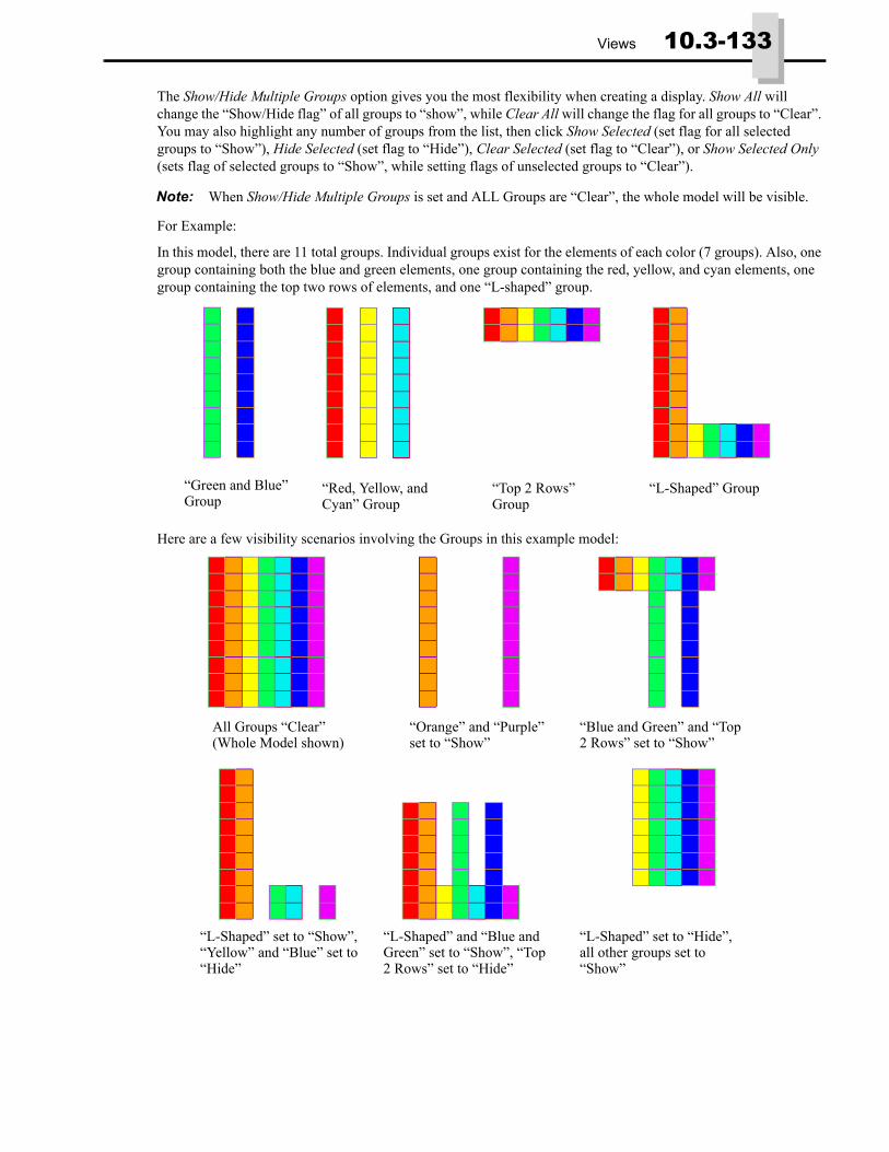
Views 10.3-133
The Show/Hide Multiple Groups option gives you the most flexibility when creating a display. Show All will change the “Show/Hide flag” of all groups to “show”, while Clear All will change the flag for all groups to “Clear”. You may also highlight any number of groups from the list, then click Show Selected (set flag for all selected groups to “Show”), Hide Selected (set flag to “Hide”), Clear Selected (set flag to “Clear”), or Show Selected Only (sets flag of selected groups to “Show”, while setting flags of unselected groups to “Clear”).
For Example:
In this model, there are 11 total groups. Individual groups exist for the elements of each color (7 groups). Also, one group containing both the blue and green elements, one group containing the red, yellow, and cyan elements, one group containing the top two rows of elements, and one “L-shaped” group.
Here are a few visibility scenarios involving the Groups in this example model:
Note: When Show/Hide Multiple Groups is set and ALL Groups are “Clear”, the whole model will be visible.
“Green and Blue” “Red, Yellow, and “Top 2 Rows” “L-Shaped” GroupCyan” Group GroupGroup
All Groups “Clear”(Whole Model shown)
“Orange” and “Purple”set to “Show”
“Blue and Green” and “Top2 Rows” set to “Show”
“L-Shaped” set to “Show”,“Yellow” and “Blue” set to
“L-Shaped” and “Blue andGreen” set to “Show”, “Top
“L-Shaped” set to “Hide”,all other groups set to
“Hide” 2 Rows” set to “Hide” “Show”
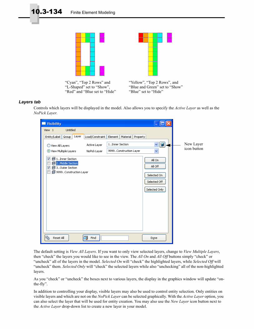
10.3-134 Finite Element Modeling
Layers tabControls which layers will be displayed in the model. Also allows you to specify the Active Layer as well as the NoPick Layer.
The default setting is View All Layers. If you want to only view selected layers, change to View Multiple Layers, then “check” the layers you would like to see in the view. The All On and All Off buttons simply “check” or “uncheck” all of the layers in the model. Selected On will “check” the highlighted layers, while Selected Off will “uncheck” them. Selected Only will “check” the selected layers while also “unchecking” all of the non-highlighted layers.
As you “check” or “uncheck” the boxes next to various layers, the display in the graphics window will update “on-the-fly”.
In addition to controlling your display, visible layers may also be used to control entity selection. Only entities on visible layers and which are not on the NoPick Layer can be selected graphically. With the Active Layer option, you can also select the layer that will be used for entity creation. You may also use the New Layer icon button next to the Active Layer drop-down list to create a new layer in your model.
“Cyan”, “Top 2 Rows” and“L-Shaped” set to “Show”,
“Yellow”, “Top 2 Rows”, and“Blue and Green” set to “Show”
“Red” and “Blue set to “Hide” “Blue” set to “Hide”
New Layericon button
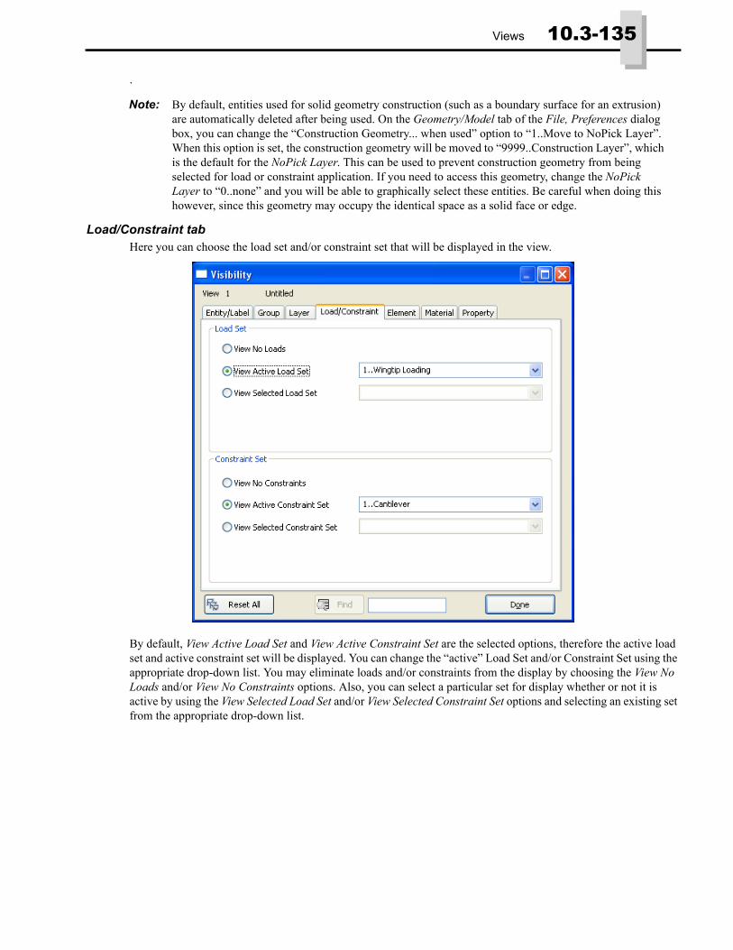
Views 10.3-135
.
Load/Constraint tabHere you can choose the load set and/or constraint set that will be displayed in the view.
By default, View Active Load Set and View Active Constraint Set are the selected options, therefore the active load set and active constraint set will be displayed. You can change the “active” Load Set and/or Constraint Set using the appropriate drop-down list. You may eliminate loads and/or constraints from the display by choosing the View No Loads and/or View No Constraints options. Also, you can select a particular set for display whether or not it is active by using the View Selected Load Set and/or View Selected Constraint Set options and selecting an existing set from the appropriate drop-down list.
Note: By default, entities used for solid geometry construction (such as a boundary surface for an extrusion) are automatically deleted after being used. On the Geometry/Model tab of the File, Preferences dialog box, you can change the “Construction Geometry... when used” option to “1..Move to NoPick Layer”. When this option is set, the construction geometry will be moved to “9999..Construction Layer”, which is the default for the NoPick Layer. This can be used to prevent construction geometry from being selected for load or constraint application. If you need to access this geometry, change the NoPick Layer to “0..none” and you will be able to graphically select these entities. Be careful when doing this however, since this geometry may occupy the identical space as a solid face or edge.

10.3-136 Finite Element Modeling
Element, Material, and Property tabsThese tabs allow you to control the visibility of elements based on Element Shape and/or Element Type (Element tab) and elements associated with specific Materials or Properties in your model.
The number of elements of each type or shape is listed after the type name or shape name when in the Element tab.
A special check box exists in the Material tab which allows you to toggle visibility on/off for “Elements with No Material” which include plot only, link, spring/damper, DOF spring, gap, laminate (reference several materials, not one), mass, mass matrix, rigid/interpolation, stiffness matrix, and slide line elements. A similar box exists in the Property tab for “Elements with No Property” which include plot only and rigid/interpolation elements.
This table describes the functions performed by each of the command buttons when in a Element, Material, or Property tab:
Only elements of shapes/types or associated with materials or properties which are currently “checked” will be available for selection in the graphics window. This can make it very easy to perform “box”, “circle”, “polygon”, or “freehand” picking of certain element types/shapes, materials, or properties.
Note: Element visibility using the Element, Material, and Property tabs applies to All Views in the model, not just the Active View like the Entity/Label, Group, Layer, and Load/Constraint tabs.
Entity/Label Button FunctionAll On “Checks” boxes for ALL element shapes/types, materials, or properties (includes
box for Elements with No Material/Property).All Off “Unchecks” boxes for all element shapes/types, materials, or properties (includes
box for Elements with No Material/Property).Selected On “Checks” boxes of highlighted element shapes/types, materials, or properties.Selected Off “Unchecks” boxes of highlighted element shapes/types, materials, or properties.Selected Only “Checks” boxes of highlighted element shapes/types, materials, or properties, while
“unchecking” boxes of shapes/types, materials, or properties which are not currently highlighted.
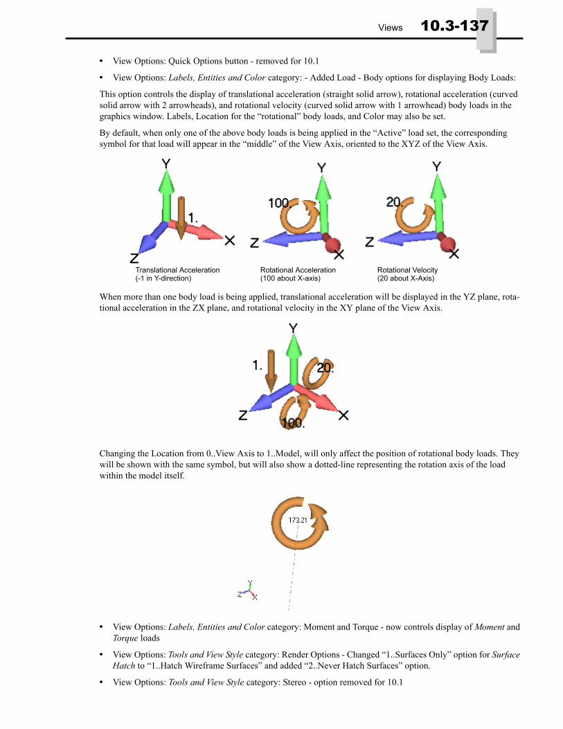
Views 10.3-137
• View Options: Quick Options button - removed for 10.1
• View Options: Labels, Entities and Color category: - Added Load - Body options for displaying Body Loads:
This option controls the display of translational acceleration (straight solid arrow), rotational acceleration (curved solid arrow with 2 arrowheads), and rotational velocity (curved solid arrow with 1 arrowhead) body loads in the graphics window. Labels, Location for the “rotational” body loads, and Color may also be set.
By default, when only one of the above body loads is being applied in the “Active” load set, the corresponding symbol for that load will appear in the “middle” of the View Axis, oriented to the XYZ of the View Axis.
When more than one body load is being applied, translational acceleration will be displayed in the YZ plane, rota-tional acceleration in the ZX plane, and rotational velocity in the XY plane of the View Axis.
Changing the Location from 0..View Axis to 1..Model, will only affect the position of rotational body loads. They will be shown with the same symbol, but will also show a dotted-line representing the rotation axis of the load within the model itself.
• View Options: Labels, Entities and Color category: Moment and Torque - now controls display of Moment and Torque loads
• View Options: Tools and View Style category: Render Options - Changed “1..Surfaces Only” option for Surface Hatch to “1..Hatch Wireframe Surfaces” and added “2..Never Hatch Surfaces” option.
• View Options: Tools and View Style category: Stereo - option removed for 10.1
Translational Acceleration Rotational Acceleration Rotational Velocity(-1 in Y-direction) (100 about X-axis) (20 about X-Axis)

10.3-138 Finite Element Modeling
Output and Post-Processing• View, Advanced Post, Contour Model Data
... allows you to view model data as contour/criteria plots or beam diagrams. This commands is not really a post-processing capability. Some common uses would be viewing a contour plot of the thicknesses of plane elements in a shell model or a criteria plot of Youngs Modulus of the materials in an assembly model using solid elements.
If you would like to display model data on elements in the graphics window, the first option to check would be Show Model Data Contour in the Contour Data From section. Next choose a single material/property data value for display by highlighting a specific value from the tree structure. Most material/property data values in FEMAP should be available for selection, with the major exceptions being the material values of the materials of the “Other Types” material type. There are 5 “special cases” which are a little more flexible with regard to the type of materi-als/properties in the model. For instance, “Plane Element Thickness” will work for any plane elements which have a thickness, including laminates. Others like “Bar/Beam/Rod Area” will allow you to show a criteria plot of areas on all the Beams/Bars/Rods in your model at once.
Once a value is chosen, you can choose to display the values as a Contour, Criteria, or Beam Diagram in the Show As section. The Allow Labels will toggle the output labels on/off for all three of the Show As options.
Finally, you can choose to plot the material/property data values on the entire model using the All option in the Show On section or only a portion of the model by choosing Group and then selecting an existing group from the drop-down list.
For example, here is a contour plot of “Plane Element Thickness” on a Shell model containing laminates of various thicknesses:

Output and Post-Processing 10.3-139
To turn off the display of material/property data values, choose the command again and UNCHECK the Show Model Data Contour check box in the Contour Data From section.
• View, Select: Contour Vectors - 2D Tensor Plot option
The 2D Tensor Plot (i.e.,“Crow’s Foot” plot) allows you to create a plot of three vectors on a 2D element. Vector 1 will be plotted in the X-direction (based on the option selected in the Output Data is Stored Relative To section), Vector 2 in the Y-direction, and Vector 3 at a 45 degree angle between the X-direction and the Y-direction. Although it may be used to show any three vectors on 2D elements, this is very useful when showing three related vectors, with two being “directional” and one being “shear”, such as Plate X Normal Stress (Vector 1), Plate Y Nor-mal Stress (Vector 2), and Plate XY Shear Stress (Vector 3).
This plot differs from the other available Vector Type plots. By default, the options set in the PostProcessing cate-gory of View Options for Vector Style and Contour Vector Style will be ignored, and the plot will be always be shown with all vectors displayed using uniform vector length, centered on the element, with output values
• View, Select: Laminate Options
Used to control the display of laminate results. By default, this option will be set to Selected Output Vector, which will simply create a contour/criteria plot using the Contour vector currently selected in the Output Vectors section of the Select PostProcessing Data dialog box. The other options are Top Ply of Layup, Bottom Ply of Layup, and Global Ply.
Note: While the Show Model Data Contour box is checked, all Contour Style settings in the View Select dia-log box (View, Select command) will be ignored until the display of model data has been turned off.
Note: If you want the 2D Tensor Plot to follow the options set in Vector Style and Contour Vector Style, simply select the File, Preferences command, choose the Views tab, then “uncheck” the “2D Tensor Plot View Options Override” option.
2D Tensor Plot showing X Normal Stress, Y Normal Stress and XY Shear Stress
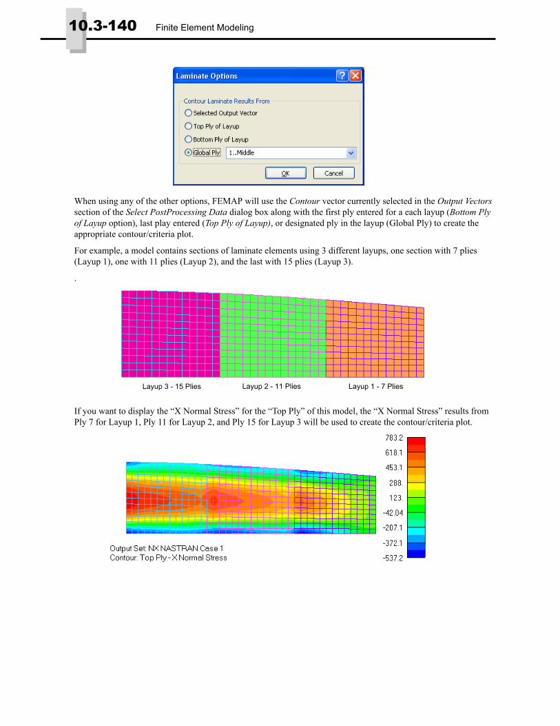
10.3-140 Finite Element Modeling
When using any of the other options, FEMAP will use the Contour vector currently selected in the Output Vectors section of the Select PostProcessing Data dialog box along with the first ply entered for a each layup (Bottom Ply of Layup option), last play entered (Top Ply of Layup), or designated ply in the layup (Global Ply) to create the appropriate contour/criteria plot.
For example, a model contains sections of laminate elements using 3 different layups, one section with 7 plies (Layup 1), one with 11 plies (Layup 2), and the last with 15 plies (Layup 3).
.
If you want to display the “X Normal Stress” for the “Top Ply” of this model, the “X Normal Stress” results from Ply 7 for Layup 1, Ply 11 for Layup 2, and Ply 15 for Layup 3 will be used to create the contour/criteria plot.
Layup 3 - 15 Plies Layup 2 - 11 Plies Layup 1 - 7 Plies

Geometry Interfaces 10.3-141
If you want to display the “X Normal Stress” for the “Bottom Ply” of this model, the “X Normal Stress” results from Ply 1 for Layup 1, Ply 1 for Layup 2, and Ply 1 for Layup 3 will be used to create the contour/criteria plot.
Finally, if you want to display the “X Normal Stress” for the “Middle Ply” of this model, you would need to desig-nate the “middle ply” of each layup using a “Global Ply”. To set up a “Global Ply”, you will need to first create a global ply in the Layup Editor, then choose a ply in each Layup and click the Update Global Ply button. See Sec-tion 4.2.5, "Model, Layup..." for more information about a global ply.
Once the Global Ply has been assigned to a ply in each layup, you can then choose it from the Global Ply drop-down list. In this case, the “X Normal Stress” results from Ply 4 for Layup 1, Ply 6 for Layup 2, and Ply 8 for Layup 3 will be used to create the contour/criteria plot.
• View Options: PostProcessing category: Contour Vector Style - Added “Exponent” Color Modes, Digits, and Length options
Geometry InterfacesThe following FEMAP interfaces have been updated to support newer geometry formats:
For details, see “Geometry Interfaces” in the FEMAP User Guide.
Analysis Program InterfacesSeveral of the analysis program interfaces have been improved. These changes include:
FEMAP Interface Latest Supported VersionParasolid Parasolid 22.0Solid Edge Solid Edge with Synchronous Technology 2NX NX 6Pro/Engineer Wildfire 4ACIS ACIS 20CATIA V5 V5 release 18SolidWorks SolidWorks 2009

10.3-142 Finite Element Modeling
• Analysis Set Manager Enhancements
• FEMAP Neutral File Interface
• NX Nastran Interface
• Nastran Interfaces (NX and MSC/MD)
• MSC/MD Nastran Interface
• NEi Nastran Interface
• ANSYS Interface
• ABAQUS Interface
• DYNA Interface
Analysis Set Manager EnhancementsFor details, see “Analysis Program Interfaces” in the FEMAP User Guide.
• Added Previous (Prev...) buttons to many of the Analysis Set Manager dialog boxes when using the Nastran Solvers.
• Enhanced Analyze and Analyze Multiple options to use internal solver queuing system when multiple jobs in one model or jobs from any number of models are sent to the solver. Queuing system now tracks which model the analysis job was launched from and will attempt to return to the correct model and import results before beginning the next analysis job. Also, added “Clear Queue” button to clear the internal queuing system.
FEMAP Neutral File Interface• Updated Neutral Read and Write for v10.1 changes
NX Nastran InterfaceA number of bugs were corrected
Solution 601 updates
• Turned the “Loads Change with Deformation” option in the Analysis Options section of NXSTRAT Solver Parameters dialog box “on” by default.
• Turned the “Constraint Force” option in the Nodal section of Nastran Output Requests dialog box “on” by default.
• Added support to SOL601 for function dependent acceleration body loads.
Solution 701 updates
• Turned the “Loads Change with Deformation” option in the Analysis Options section of NXSTRAT Solver Parameters dialog box “on” by default.
• Turned the “Constraint Force” option in the Nodal section of Nastran Output Requests dialog box “on” by default.
For details, see “Analysis Program Interfaces” in the FEMAP User Guide.
Nastran Interfaces (NX and MSC/MD)• Turned off PARAM,MAXRATIO by default
• Added support to read the CVISC and PVISC entries
• Added support to read and write PARAM,RESVINER
• Added support to read and write LOAD, SPCADD, and MPCADD entries
• Added support to set the All Plates as QUADR/TRIAR option when CQUADR and CTRIAR elements are imported
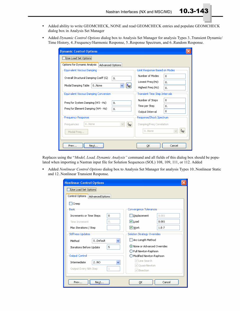
Nastran Interfaces (NX and MSC/MD) 10.3-143
• Added ability to write GEOMCHECK, NONE and read GEOMCHECK entries and populate GEOMCHECK dialog box in Analysis Set Manager
• Added Dynamic Control Options dialog box to Analysis Set Manager for analysis Types 3..Transient Dynamic/Time History, 4..Frequency/Harmonic Response, 5..Response Spectrum, and 6..Random Response.
Replaces using the “Model, Load, Dynamic Analysis” command and all fields of this dialog box should be popu-lated when importing a Nastran input file for Solution Sequences (SOL) 108, 109, 111, or 112. Added
• Added Nonlinear Control Options dialog box to Analysis Set Manager for analysis Types 10..Nonlinear Static and 12..Nonlinear Transient Response.

10.3-144 Finite Element Modeling
Replaces using the “Model, Load, Nonlinear Analysis” command and all fields of this dialog box should be popu-lated when importing a Nastran input file for Solution Sequences (SOL) 106 or 129, when an NLPARM entry exists.
• Added support to read DLOAD, NONLINEAR, TSTEP, TSTEPNL, NLPARM, SDAMPING, FREQUENCY, RANDOM Case Control entries
• Added support to read PARAMs LMODES, LFREQ, HFREQ, W3, W4, G, RSPECTRA, SCRSPEC, OPTION (ABS, SRSS, NRL, NRLO), CLOSE, LANGLE
• Added support to read TSTEP, TSTEPNL, NLPARM, NLPCI, RANDPS, DTI Bulk Data entries
A number of bugs were corrected
For details, see “Analysis Program Interfaces” in the FEMAP User Guide.
MSC/MD Nastran InterfaceA number of bugs were corrected.
For details, see “Analysis Program Interfaces” in the FEMAP User Guide.
NEi Nastran Interface• Added support to read PARAM,OPTION,CQC
A number of bugs were corrected.
For details, see “Analysis Program Interfaces” in the FEMAP User Guide.
ANSYS InterfaceA number of bugs were corrected.
For details, see “Analysis Program Interfaces” in the FEMAP User Guide.
ABAQUS InterfaceA number of bugs were corrected.
For details, see “Analysis Program Interfaces” in the FEMAP User Guide.
DYNA Interface• Added support 8-noded Quad elements
• Added support for nonstructural mass for Beam and Shell elements
• Added support for the following element formulations:
Fully Integrated DKT triangular, Fully Integrated linear DK quadrilateral, Fully Integrated linear assumed strain C0, 1 point Eulerian Navier-Stokes, 8 point Eulerian Navier-Stokes, and CVFEM Eulerian Navier-Stokes
A number of bugs were corrected.
For details, see “Analysis Program Interfaces” in the FEMAP User Guide.
OLE/COM APINew API Objects and Attributes• Added NasBulkDynLdAsLOADSET, NasBulkResViner, NasGCheckNone, NasBulkWriteAllLoadBCSets,
NasDynOn, NasDynUseLoadSet, NasDynDampOverall, NasDynDampW3, NasDynDampW4, vNasDynKeep-Freq, NasDynTranDT, NasDynFreqTbl, NasDynDampModalTbl, NasDynKeepModes, NasDynTran-TimeSteps, NasDynTransOutInt, NasDynDampModalMethod, NasDynRespSpect, vNasDynNoFreq, vNasDynLogInterp, vNasDynFreqType, vNasDynMinFreq, vNasDynMaxFreq, and vNasDynSpreadCluster to AnalysisMgr object

OLE/COM API 10.3-145
• NasCnlIncrements, NasCnlTime_Increment, NasCnlMaxIter, vNasCnlConvergenceFlags, vNasCnlConver-genceValue, NasCnlCtiffnessMethod, NasCnlKstep, NasCnlIntermediateOutput, NasCnlOutputInterval, NasCnlSolutionStrategy, NasCnlSolutionOverrides, NasCnlModnewtonLineSearch, NasCnlModnewton-QuasiNewton, NasCnlModnewtonBisection, NasCnlArcConstraintType, NasCnlArcMinAdjust, NasCnlArc-MaxAdjust, NasCnlArcLoadScale, NasCnlArcDesiredIter, NasCnlArcMaxSteps, NasCnlTimeSkipAdjust, NasCnlDominantPeriodSteps, NasCnlBoundsRb, NasCnlStabilityTolerance, NasCnlDivergenceLimit, NasCn-lQuasiNewtonVectors, NasCnlMaxLineSearch, NasCnlCreep, NasCnlLineSearchTolerance, NasCnlMaxBisec-tions, NasCnlMaxRotation, NasCnlFstress, and NasCnlMaxAdjust to AnalysisMgr object.
• Added IsCombination to LoadSet object.
• Added Gradient to LoadETemp object.
• Added IsCombination to BCSet object
• Added GlobalPlyLocation to View object.
New API Methods• Added AddCoordinate, AddAroundPoint, AddAroundVector, AddAroundPlane, AddNodesOnGeometry, and
SelectList methods for Set object
• Added RemoveSet, ConvertToBoundarySurfaces, and SelectListmethods for Sort object
• Added ClearAnalysisQueue, GetCorrelate2, and PutCorrelate2 methods forAnalysisMgr object
• Added GetDataSurfType method for DataSurf object
• Added PartialLengthXYZ, PartialLengthNode, and SelectList methods for Curve object
• Added IsBoundingSolidRegion, Mesh, and ResetMeshAttr methods for Surface object
• Added IsGeneral method for Solid object
• Added GetClosest method for Node object
• Added Thickness, Area, and Inertia methods for Elem object
• Added Thickness, Area, and Inertia methods for Prop object
• Added GetCombination and PutCombination methods for LoadSet object
• Added GetCombination and PutCombination methods for BCSet object
• Added ReferencedGroups method for Group object
• Added DefineReal method for Var object
• Added GetMultiGroupList, SetMultiGroupList, and ClearMultiGroupList methods for View object
• Added InitScalarAtBeam and PutScalarAtBeam methods for Output object
• Added Reverse method for Contact and ConnectionRegion objects
New Global Variables• Added Pref_NastranUseILP64, Pref_ConstructionGeometry, and Pref_NastranWriteAllLdbcSets
• Added FLT_SNTORQUE for Load Type
• Added FVD_AXIS_OF_SURFACE for Vector Definition Method
The following functions have been added:• feSurfaceRemoveHole
• feModifySolidFacetting
• feSolidRemoveFace
• feMeshSurface2
• feAppRegisterAddInPaneWithFrame
• feVectorAxisOfSurface
10.3-146 Finite Element Modeling
• feMeshSurfaceByAttributes
PreferencesViews• Added 2D Tensor Plot View Options Override option.
This option is on by default. When viewing contour vectors using the 2D Tensor Plot option, the options set in the PostProcessing category of View Options for Vector Style and Contour Vector Style will be ignored, and the plot will be always be shown with all vectors displayed using uniform vector length, centered on the element, with out-put values
Database• Added Open/Save Method option.
This option should only be used if you are experiencing VERY slow opening/saving FEMAP model files. On cer-tain hardware, switching to option “2..64K widows I/O” may make a dramatic difference in the time a model takes to open/save. Essentially, what option 2 does is copy to (opening) and from the scratch directory (saving) in 64K “blocks” instead of allowing the hardware to choose the size. Options 1 and 3 are simply other alternatives to try.
Interfaces• Added Use ILP-64bit NX Nastran option.
If you have NX Nastran installed on a 64-bit system, this option will instruct NX Nastran to solve using the “ILP” version of 64-bit Nastran. “ILP” is able to allocate more memory than “regular” 64-bit NX Nastran by using a 64-bit word size and 64-bit memory pointer, while integers are 64-bits and floating point uses one 64-bit word.
• Added Write All Static Load/BC Sets option.
When this option is on, FEMAP will write ALL loads and constraint sets to the Nastran input file for Linear Static Analysis. This essentially forces FEMAP to write out Nastran input files for SOL 101 the way it has in all versions before FEMAP 10.1.