Female labor force participation

Heidi L. WilliamsMIT 14.662Spring 2015

Outline

1) Goldin (2006) Ely lecture

2) Compensating differentials:

Goldin (2014), Bertrand et al. (2010), Goldin and Katz (forthcoming)

3) Roy model: Mulligan and Rubinstein (2008)

1 Facts: Goldin (2006)

Goldin argues that the most significant change in labor markets over the past century was the

increased participation of women in the labor market. Figure 1 summarizes historical trends in

mens’ and womens’ labor force participation.

Courtesy of Claudia Goldin and the AmericanEconomic Association. Used with permission.

1

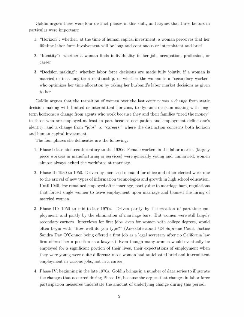
Goldin argues there were four distinct phases in this shift, and argues that three factors in

particular were important:

1. “Horizon”: whether, at the time of human capital investment, a woman perceives that her

lifetime labor force involvement will be long and continuous or intermittent and brief

2. “Identity”: whether a woman finds individuality in her job, occupation, profession, or

career

3. “Decision making”: whether labor force decisions are made fully jointly, if a woman is

married or in a long-term relationship, or whether the woman is a “secondary worker”

who optimizes her time allocation by taking her husband’s labor market decisions as given

to her

Goldin argues that the transition of women over the last century was a change from static

decision making with limited or intermittent horizons, to dynamic decision-making with long-

term horizons; a change from agents who work because they and their families “need the money”

to those who are employed at least in part because occupation and employment define one’s

identity; and a change from “jobs” to “careers,” where the distinction concerns both horizon

and human capital investment.

The four phases she delineates are the following:

1. Phase I: late nineteenth century to the 1920s. Female workers in the labor market (largely

piece workers in manufacturing or services) were generally young and unmarried; women

almost always exited the workforce at marriage.

2. Phase II: 1930 to 1950. Driven by increased demand for office and other clerical work due

to the arrival of new types of information technologies and growth in high school education.

Until 1940, few remained employed after marriage, partly due to marriage bars, regulations

that forced single women to leave employment upon marriage and banned the hiring of

married women.

3. Phase III: 1950 to mid-to-late-1970s. Driven partly by the creation of part-time em-

ployment, and partly by the elimination of marriage bars. But women were still largely

secondary earners. Interviews for first jobs, even for women with college degrees, would

often begin with “How well do you type?” (Anecdote about US Supreme Court Justice

Sandra Day O’Connor being offered a first job as a legal secretary after no California law

firm offered her a position as a lawyer.) Even though many women would eventually be

employed for a significant portion of their lives, their expectations of employment when

they were young were quite different: most woman had anticipated brief and intermittent

employment in various jobs, not in a career.

4. Phase IV: beginning in the late 1970s. Goldin brings in a number of data series to illustrate

the changes that occurred during Phase IV, because she argues that changes in labor force

participation measures understate the amount of underlying change during this period.

2

She argues that women more accurately anticipated their future working lives, using data

from the National Longitudinal Survey (NLS) of Young Women, which asked questions about

expectations of paid employment at age 35. As shown in Figure 2, young woman in the 1970s

began with expectations similar to the actual participation of their mothers’ generation (around

0.3), but in the next ten years began to correctly anticipate - and slightly overstate - their future

labor force participation rates.

Courtesy of Claudia Goldin and the AmericanEconomic Association. Used with permission.

3

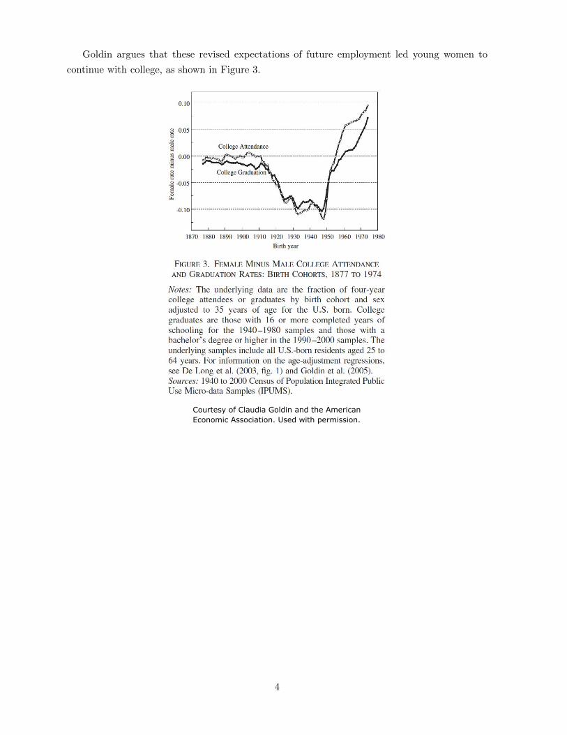
Goldin argues that these revised expectations of future employment led young women to

continue with college, as shown in Figure 3.

Courtesy of Claudia Goldin and the AmericanEconomic Association. Used with permission.

4

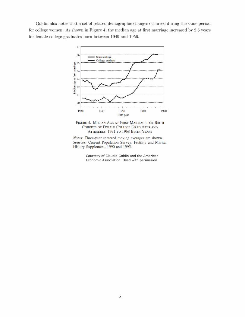
Goldin also notes that a set of related demographic changes occurred during the same period

for college women. As shown in Figure 4, the median age at first marriage increased by 2.5 years

for female college graduates born between 1949 and 1956.

Courtesy of Claudia Goldin and the AmericanEconomic Association. Used with permission.

5

Women also began to further their education in professional and graduate schools around

1970, as shown in Figure 5.

Courtesy of Claudia Goldin and the AmericanEconomic Association. Used with permission.

6

The earnings of women relative to men began to increase around 1980, after remaining flat

since the 1950s, as shown in Figure 7.

Occupations shifted from “traditional” women’s occupations to a more varied group, as

shown in Figure 8.

Courtesy of Claudia Goldin and the AmericanEconomic Association. Used with permission.

Courtesy of Claudia Goldin and the AmericanEconomic Association. Used with permission.

7

Goldin’s discussion of the potential drivers of these Phase IV changes focuses on several

factors. First, women in these cohorts observed the large increase in participation and full-time

work of their predecessors, and extrapolated from that more accurate expectations for their

futures. In doing so, they were better prepared to invest in their human capital. Marriage delay

enabled women to take formal education more seriously, and she argues that one underlying

driver of this marriage delay was the introduction of the contraceptive “pill.” While the pill was

FDA approved in 1960, restrictive state laws were in place until the late 1960s and early 1970s.

2 Compensating differentials:

Goldin (2014), Bertrand et al. (2010), Goldin and Katz (forthcoming)

2.1 Goldin (2014)

Goldin’s 2014 AEA Presidential address follows on her Ely lecture, with a focus on the con-

vergence in earnings between men and women. Figure 1 plots the earnings gender gap by age

using synthetic birth cohorts (for college graduates working full-time full-year). The two striking

findings from this graph are that each cohort has a higher ratio of female to male earnings than

the preceding one, and that the ratio is closer to parity for younger individuals than for older

individuals, up to some age, but the ratio increases again when individuals are in their forties.

The main conclusion she draws from this is that differences in earnings by sex greatly increases

during the first several decades of working life.

8

Courtesy of Claudia Goldin and the American Economic Association. Used with permission.

9

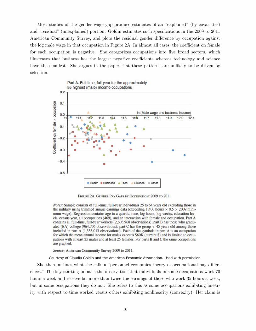
Most studies of the gender wage gap produce estimates of an “explained” (by covariates)

and “residual” (unexplained) portion. Goldin estimates such specifications in the 2009 to 2011

American Community Survey, and plots the residual gender difference by occupation against

the log male wage in that occupation in Figure 2A. In almost all cases, the coefficient on female

for each occupation is negative. She categorizes occupations into five broad sectors, which

illustrates that business has the largest negative coefficients whereas technology and science

have the smallest. She argues in the paper that these patterns are unlikely to be driven by

selection.

Courtesy of Claudia Goldin and the American Economic Association. Used with permission.

She then outlines what she calls a “personnel economics theory of occupational pay differ-

ences.” The key starting point is the observation that individuals in some occupations work 70

hours a week and receive far more than twice the earnings of those who work 35 hours a week,

but in some occupations they do not. She refers to this as some occupations exhibiting linear-

ity with respect to time worked versus others exhibiting nonlinearity (convexity). Her claim is

10

that when earnings are linear with respect to time worked the gender gap is low; when there is

nonlinearity the gender gap is higher.

While total hours worked are relevant, she notes that often what counts are the particular

hours worked. The employee who is around when others are as well may be rewarded more than

the employee who leaves at 11am for two hours but is hard at work for two additional hours in

the evening.

In many workplaces, employees meet with clients and accumulate knowledge about them. If

an employee is unavailable and communicating the information to another employee is costly,

the value of the individual to the firm will decline. Equivalently, employees often gain from

interacting with each other in meetings or through random exchanges.

Her key point is that whenever an employee does not have a perfect substitute, nonlinearities

can arise. When there are perfect substitutes for particular workers and zero transaction costs,

there is never a premium in earnings with the respect to the number or the timing of hours. If

there were perfect substitutes earnings would be linear with respect to hours.

2.2 MBAs: Bertrand, Goldin and Katz (2010)

Despite the narrowing of the gender gap in business education, there is a growing sense that

women are not getting ahead fast enough in the corporate and financial world. There is ex-

perimental evidence that women have less taste for the highly-competitive environments in top

finance and corporate jobs. Women may also fall behind because of the career/family conflicts

arising from the purportedly long hours, heavy travel commitments, and inflexible schedules of

most high-powered finance and corporate jobs.

Although male and female MBAs have nearly identical earnings at the outset of their careers,

Bertrand et al. (2010) find their earnings soon diverge, with the male earnings advantage reaching

almost 60 log points a decade after MBA completion. The authors argue that three proximate

factors account for the large and rising gender gap in earnings: differences in training prior to

MBA graduation, differences in career interruptions, and differences in weekly hours.

2.2.1 Data

The authors conducted web-based surveys of University of Chicago MBAs from the graduating

classes of 1990 to 2006. The participants were asked detailed questions about each of the jobs

or positions they had since graduation, including earnings (both at the beginning and end of a

given position), usual weekly hours worked, job function, sector, size of firm, and type of firm.

The authors collected administrative data from the University of Chicago to match to the

survey data, providing information on MBA courses and grades, under- graduate school, under-

graduate GPA, GMAT scores, and demographic information (age, ethnicity, and immigration

status).

Among the MBAs in these classes with known e-mail addresses, about 31 percent responded

to the survey. Of this group, 2,485 (or 97 percent) were matched to University of Chicago

11

administrative records. These 1,856 men and 629 women form the basis of their sample. The

respondents do not differ much from the nonrespondents based on the observables.

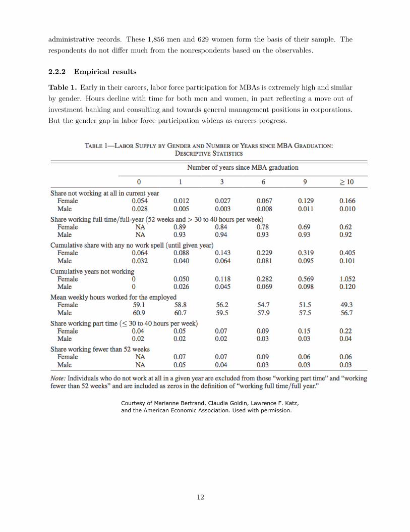
2.2.2 Empirical results

Table 1. Early in their careers, labor force participation for MBAs is extremely high and similar

by gender. Hours decline with time for both men and women, in part reflecting a move out of

investment banking and consulting and towards general management positions in corporations.

But the gender gap in labor force participation widens as careers progress.

Courtesy of Marianne Bertrand, Claudia Goldin, Lawrence F. Katz,and the American Economic Association. Used with permission.

12

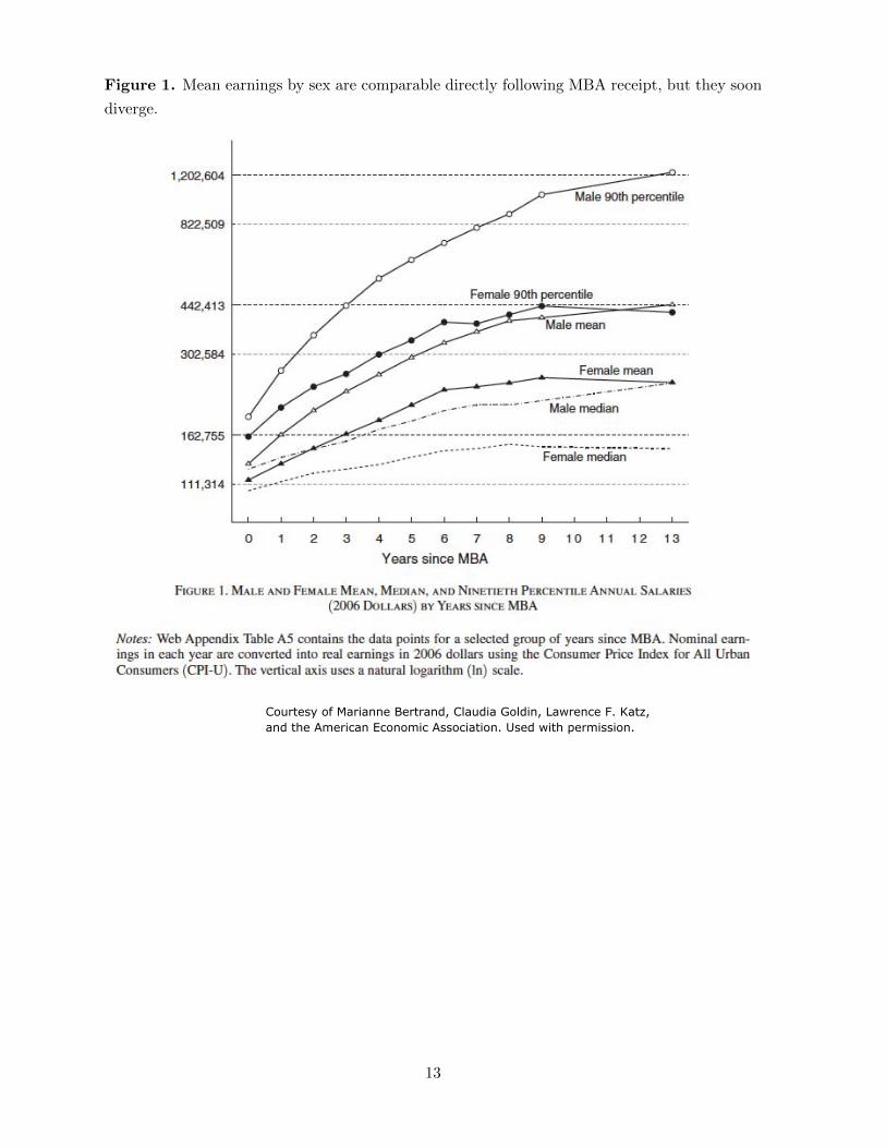
Figure 1. Mean earnings by sex are comparable directly following MBA receipt, but they soon

diverge.

Courtesy of Marianne Bertrand, Claudia Goldin, Lawrence F. Katz,and the American Economic Association. Used with permission.

13

Table 4. Differences in three factors - MBA performance (24%; GPA and finance courses),

career interruptions and job experience (30%), and hours worked (30%) - account for 84 percent

of the gender gap in earnings pooled across all years since MBA completion.

Courtesy of Marianne Bertrand, Claudia Goldin, Lawrence F. Katz,and the American Economic Association. Used with permission.

Perhaps unsurprisingly, children appear to be a main contributor to women’s labor supply

changes. Women with children work 24% fewer hours per week than men or than women without

children. The association between children and female labor supply differs strongly by spousal

income, with MBA moms with high-earning spouses having labor force participation rates that

are 18.5 percentage points lower than those with lesser-earning spouses.

14

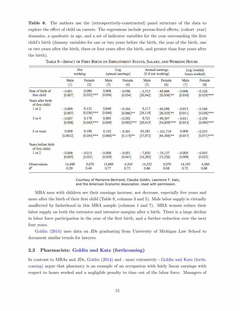
Table 8. The authors use the (retrospectively-constructed) panel structure of the data to

explore the effect of child on careers. The regressions include person-fixed effects, (cohort year)

dummies, a quadratic in age, and a set of indicator variables for the year surrounding the first

child’s birth (dummy variables for one or two years before the birth, the year of the birth, one

or two years after the birth, three or four years after the birth, and greater than four years after

the birth).

Courtesy of Marianne Bertrand, Claudia Goldin, Lawrence F. Katz,and the American Economic Association. Used with permission.

MBA men with children see their earnings increase, not decrease, especially five years and

more after the birth of their first child (Table 8, columns 3 and 5). Male labor supply is virtually

unaffected by fatherhood in this MBA sample (columns 1 and 7). MBA women reduce their

labor supply on both the extensive and intensive margins after a birth. There is a large decline

in labor force participation in the year of the first birth, and a further reduction over the next

four years.

Goldin (2014) uses data on JDs graduating from University of Michigan Law School to

document similar trends for lawyers.

2.3 Pharmacists: Goldin and Katz (forthcoming)

In contrast to MBAs and JDs, Goldin (2014) and - more extensively - Goldin and Katz (forth-

coming) argue that pharmacy is an example of an occupation with fairly linear earnings with

respect to hours worked and a negligible penalty to time out of the labor force. Managers of

15

pharmacies get paid more because they work more hours. Female pharmacists get paid less

because they work fewer hours. But there is no “part time penalty.”

Goldin and Katz (forthcoming) study closely how pharmacy became the most egalitarian

profession over the time period 1970-2010. The authors argue that three production and health-

care changes are the forces behind the evolution of the pharmacy sector - technological changes

increasing the substitutability among pharmacists, the growth of pharmacy employment in retail

chains and hospitals, and the related decline of independent pharmacies.

1. Drug stores have increased in their scope and scale since 1970. These changes led to a

greater share of corporate-owned pharmacies (e.g., CVS, Walgreens and Rite-Aid) and a

lower share of owner-operated pharmacies, against a backdrop of evolution of retail chain

stores. Owner-operated pharmacies demand more hours of work whereas in corporate-

owned pharmacies the hours are more flexible. Changes in the healthcare sector led to an

increase of pharmacists working in hospitals and mail-order pharmacies.

2. Demand-side substitutability. Pharmacists can access the prescriptions of clients through

electronic systems administered by the Pharmacy Benefit Manager, so there is less cost/friction

when pharmacists handoff clients.

3. Standardization of pharmacy products and services. Medicines have been increasingly pro-

duced by pharmaceutical companies, rather than being compounded in individual phar-

macies. As a result, the idiosyncratic expertise of a particular pharmacist have become

less important.

Over time, the demand for pharmacists has grown. The authors outline a compensating

differentials framework along the lines of Goldin (2014) to clarify two cases. First, a demand

side shift raising the demand for an amenity would imply an increase in the cost of the amenity

and hence a likely decline in women’s relative earnings. In contrast, a supply side shift lowering

the cost to firms of providing the amenity implies a decrease in the cost of the amenity and

hence a likely increase in women’s relative earnings. They argue that the data and institutional

context are more consistent with the latter than the former.

Unfortunately, the paper does little to tease apart the potential channels proposed by the

authors. Doing so would seem to require either going beyond a case study of one profession, or

using cross-geography variation in the three mechanisms.

Goldin (2014) concludes her paper by arguing that there are many occupations and sectors

that have moved in the direction of less costly flexibility (physicians are a good example). But

she stresses that not all positions can be changed.

16

3 Roy model: Mulligan and Rubinstein (2008)

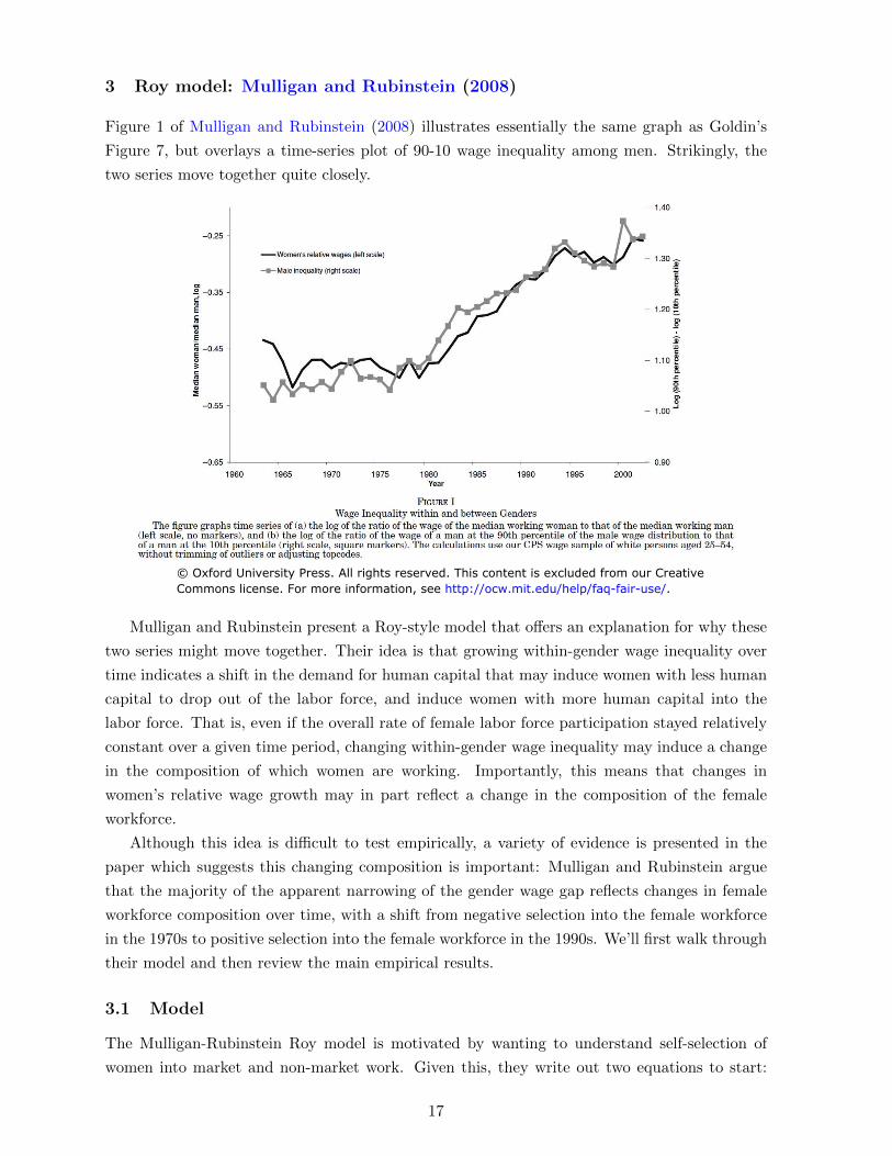
Figure 1 of Mulligan and Rubinstein (2008) illustrates essentially the same graph as Goldin’s

Figure 7, but overlays a time-series plot of 90-10 wage inequality among men. Strikingly, the

two series move together quite closely.

© Oxford University Press. All rights reserved. This content is excluded from our CreativeCommons license. For more information, see http://ocw.mit.edu/help/faq-fair-use/.

Mulligan and Rubinstein present a Roy-style model that offers an explanation for why these

two series might move together. Their idea is that growing within-gender wage inequality over

time indicates a shift in the demand for human capital that may induce women with less human

capital to drop out of the labor force, and induce women with more human capital into the

labor force. That is, even if the overall rate of female labor force participation stayed relatively

constant over a given time period, changing within-gender wage inequality may induce a change

in the composition of which women are working. Importantly, this means that changes in

women’s relative wage growth may in part reflect a change in the composition of the female

workforce.

Although this idea is difficult to test empirically, a variety of evidence is presented in the

paper which suggests this changing composition is important: Mulligan and Rubinstein argue

that the majority of the apparent narrowing of the gender wage gap reflects changes in female

workforce composition over time, with a shift from negative selection into the female workforce

in the 1970s to positive selection into the female workforce in the 1990s. We’ll first walk through

their model and then review the main empirical results.

3.1 Model

The Mulligan-Rubinstein Roy model is motivated by wanting to understand self-selection of

women into market and non-market work. Given this, they write out two equations to start:

17

a potential market wage equation and a nonmarket wage equation. Let woman i’s date t log

reservation wage rit be:

rit = µrt + σrt εrit (1)

and let her date t log potential wage (if working) wit be:

wit = µwt + γt + σwt εwit (2)

As in the Borjas model, these expressions decompose wages into the part explained by observable

characteristics (µwt and µrt ) and the part explained by unobserved characteristics (εwit and εrit).

The εwit and εrit terms are normalized to have mean zero and standard deviation 1: εwit N(0, 1)

and εr∼

it ∼ N(0, 1). Note that this implicitly assumes that the underlying skill distributions are

time-invariant. The unobserved factors are weighted by either market (σwt ) or non-market (σrt )

prices.

Woman i will choose to work at time t (Lit = 1) ⇐⇒ wit > rit, which is trueσwt ε

wit

⇐⇒r − εrit > −

γ( t+µwt −µrt

r ). Mulligan and(Rubinstein) (focus on the case where εw rit and εσ it follow a

t σtεw

standard bivariate normal distribution: itεr ∼ 1 ρN ( 0

0 ) , ρ 1 . Note that this assumes thatit

the cross-sectional correlation between log reservation wages

(and

))log potential market wages, ρ,

is constant over time.

Mulligan and Rubinstein focus on the case in which all men work but not all women work,

implying that the actual gender gap γt differs from the gender gap observed in the data. Theyσw

derive an expression for the observed gender gap as follows. Let ν t εwit r

it = εσrt− it. The derivation

here is very similar to what we worked out before for the Borjas model; in particular, recall thatσ

E (ε |v) = 0,v0 2 v. The observed gender gap Gt can then be written as:

σv (σwεw

Gt = γt + E σwt εwit| t it γ

σr− εr t + µwt µrt

it >−−( )

t σrt

)(3)

w r

= γ + σwE

(εw

γt + µt µtt t it >

−|νit −( )σrt

)(4)

γt + µw µr= γt + σw (εwt E

(E it|ν t t

it) |νit > −(−

)σrt

)(5)

w r,νw

(σεwit it γ| − t + µ µ

= γt + σt E νit νit > ( t − t )σ2νit σrt

)(6)

σw w w rt σε ,ν νit νit γt + µ µ

= γ E tt + it it

> ( (7)νit

(−

σνit| t )

σ σ rνit

−σνitσt

σ w

)w,ν µrε σ wε ,ν γ +µ

Recall that σεw = 1, so that ρ itwν = it = it it . We can rewrite E νit νit > ( t t − t )

it 1·σ rν σν σν σνit it

|it

− σν σit it t

φ(−δt) γt+µw r

as where δ t t( t =−µr . Interchanging φ( δt) = φ(δt) and rewriting 1 Φ( δt) = Φ(δt)1 Φ( δt) σν σ −

(− −

)− − it t

w r

implies that E νit γ>

ν| νit µσνit

−( t+ t −µtσ σν σr )

it it t

)φ(δcan be simplified to λ(δt) = t) . We then have:Φ(δt)

18

Gt = γt + σwt ρwνλ(δt) (8)

The second term in this expression is the selection bias term weighted by market prices σwt .σwεw

It is useful to derive an expression for σεw,νit it . Because νit = t itσr εrit, we know that νitt− ∼

σw 2 2ρσwN

(0, 1 +

(tr

)− t

r

). We can then derive ρwν as follows:σt σt

σεw,νit = cov (νit, εw

it it) (9)

= cov

(σwt ε

wit − εr , εw (10)

σr it itt

)= cov

(σw wt εit , εw

)− cov (εr , εw)

σr it it it (11)t

σw= t var (εw

σr it)t

− cov (εrit, εwit) (12)

σw= t ρ (13)

σrt−

2σw 2 w

Substituting σ t ρσtν wr rit = 1 + σεσ − and the expression for ,νσ it it from above into ρwν =

t tσ wε ,νit it , we have:

√σ

( )νit

Gt = γt + σwt

σwtσrt− ρ

λ(δt) (14)σw 2 1 t 2ρσw

+ t

σrt σrt

w

−σ

t

√ ρ

Let b √ r

denote the σ−

( ) t

t ( w w

)2 λ(δt) expression, which is a selection bias term (weighted

σ 2ρσ1+ t

rσt− t

rσt

in the Gt expression by market prices σwt ). Selection bias will be positive only if the numerator inσw

this expression is positive (that is, if tr >t−ρ 0). Hence, the sign of self-selection depends on theσσw

ratio of market to non-market prices ( t ) and the correlation between market and non-marketσrt

skills (ρ). This analogues the Borjas model, where self-selection depending relative inequality

and the correlation of ability in the two settings.

Mulligan and Rubinstein then look at how selection changes with changes in the ratio of

market to non-market prices, and show that (∂btwσ )∣∣∣∣∣ > 0. This comparative static says

∂ trσt dλt=0

that an increase in market prices relative to non-market prices increases selection bias: if bt is

negative, it becomes less negative; if bt is positive, it becomes more positive. They also derive a

second comparative static of how bt changes with changes in λ(δt). The sign of this comparative

static can be positive or negative: if self-selection is negative, increases in female labor force

participation will increase female wages; on the other hand, if self-selection is positive, increases

in female labor force participation will decrease female wages.

19

3.2 Data and estimation

Mulligan and Rubinstein use the March Current Population Survey (CPS) files in a series of

empirical specifications; we here focus on their two main specifications: a Heckman two-step

estimator, and an identification at infinity analysis. Recovering the latent gender gap - the goal

of these exercises - is difficult, and neither of these strategies is perfect.

The Heckman two-step estimator follows directly from the Roy model (taking seriously the

normality assumption). Mulligan and Rubinstein estimate a probit model of female labor force

participation as a function of demographic characteristics (Xit) and an excluded instrument (the

number of children aged 0-6 interacted with marital status); Zit denotes Xit together with the

excluded instrument:

Pt(Zit) = Φ(Zitδt) = Prob(work|Zit, female) (15)

Pt(Zit) are estimated as the fitted values from this probit equation, estimated on a sample

of women; Pt(Zit) is set to 1 for men. Then, on the sample of employed men and women, theyφ(Z δ )estimate log wages as a function of Xit and the Inverse Mills Ratio λ(Zitδt) = it t :Φ(Zitδt)

wit = Xitβt + giγt + giθtλ(Zitδt) + uit (16)

Even if you don’t use the Heckman two-step estimator in your own research, it is important

that you are literate in this method and understand its strengths and weaknesses. In short,

in the absence of an excluded instrument the Heckman correction lives off a functional form

assumption: the Inverse Mills Ratio is a non-linear function of the same Xit that are included

linearly in the second (wage) regression. Here, Mulligan and Rubinstein use an instrument, but

the exclusion restriction is not very plausible. These concerns are what motivate the second

(identification at infinity) strategy.

The Roy model suggests that selection bias disappears for groups with characteristics Xit

such that practically all individuals work, even dropping the normality assumption. This ob-

servation motivates an identification at infinity method which estimates the wage equation on a

sample selected such that almost all of the sample works. Mulligan and Rubinstein implement

this method by estimating a probit equation for labor force participation separately by gender as

a function from the Xit’s above and a vector of coefficients for gender. The purpose of this probit

model is to select which demographic groups to include in the wage equation: they include only

men and women who are employed and who have demographic characteristics such that their

predicted probability of employment α is close to one. In practice, they show results for several

α’s. A selection-corrected gender wage gap is then calculated as the conditional gender wage

gap for this selected sample. This method essentially predicts female labor force participation

as a function of a bunch of stuff including schooling. But schooling is a choice variable, and we

know that the selection of women vs. men into higher education levels has changed over time,

so it seems unlikely that comparing (essentially) the wage gap between highly educated men

20

and highly education women over time is “taking care of” selection given the changing selection

into education over time (differentially by gender).

3.3 Results

Mulligan and Rubinstein’s main results are summarized in Figure VI. The Heckman two-step

and identification at infinity strategies give similar results: both suggest the latent gender wage

gap has barely changed since 1975.

In terms of key take-aways, I would stress two. First, both of the empirical strategies here

leave room for improvement, in the sense that assumptions underlying each approach seem

unlikely to hold. Second, substantively this is an incredibly important question, and taken at

face value this is a very thought-provoking set of results. If we think that in fact there has been

little to no change in the latent gender wage gap over time, that provides a very different picture

of how women are faring in the labor force relative to if we thought that womens’ wages were

converging towards mens’ wages over time.

References

Bertrand, Marianne, Claudia Goldin, and Lawrence Katz, “Dynamics of the gender gap amongyoung professionals in the corporate and financial sectors,” American Economic Journal: AppliedEconomics, 2010, 2 (3), 228–255.

21

É Oxford University Press. All rights reserved. This content is excluded from our CreativeCommons license. For more information, see http://ocw.mit.edu/help/faq-fair-use/.

Goldin, Claudia, Understanding the Gender Gap: An Economic History of American Women, OxfordUniversity Press, 1990.

, “Richard T. Ely lecture: The quiet revolution that transformed women’s employment, education,and family,” American Economic Review, 2006, 96 (2), 1–21.

, “AEA Presidential Address: A grand gender convergence, Its last chapter,” American EconomicReview, 2014, 104 (4), 1091–1119.

and Lawrence Katz, “The most egalitarian profession: Pharmacy and the evolution of a family-friendly occupation,” Journal of Labor Economics, forthcoming.

Mulligan, Casey and Yona Rubinstein, “Selection, investment, and women’s relative wages overtime,” Quarterly Journal of Economics, 2008, 123 (3), 1061–1110.

22

MIT OpenCourseWarehttp://ocw.mit.edu

14.662 Labor Economics IISpring 2015

For information about citing these materials or our Terms of Use, visit: http://ocw.mit.edu/terms.