FEM: A Basic Overview of the Method & Outlook on Applications
92
Max-Planck-Institut für Eisenforschung, Düsseldorf, Germany 1 FEM: A Basic Overview of the Method & Outlook on Applications William Counts Max-Planck-Institut für Eisenforschung, Düsseldorf , August 25, 2008, Aachen
Transcript of FEM: A Basic Overview of the Method & Outlook on Applications

Max-Planck-Institut für Eisenforschung, Düsseldorf, Germany
1
FEM: A Basic Overview of the Method & Outlook on Applications
William Counts
Max-Planck-Institut für Eisenforschung, Düsseldorf
, August 25, 2008, Aachen

Max-Planck-Institut für Eisenforschung, Düsseldorf, Germany
2
Introduction
FEM: Finite Element Method
A great picture generating tool!!!!
MORE THAN JUST COMPUTER GENERATED ART

Max-Planck-Institut für Eisenforschung, Düsseldorf, Germany
3
Put the solution
pieces together to form global solution
Make simple
approximation of solution for each piece
Decompose
problem into pieces
Problem
(usually partial differential equation)
FEM Solution
My view: FEM is a mathematical tool.
Any physically meaningful output MUST result from physical
input provided by you to FEM

Max-Planck-Institut für Eisenforschung, Düsseldorf, Germany
4
Example: Computing the circumference of a circle with radius r
Node
Node
Element
!! Decompose (or Discretize) the problem
6 Elements 8 Elements 14 Elements
!! Approximate solution for each piece (or element)
!! Assemble the Element Equations and Solve
Ne = 6 Pc = 6.00 r
Ne = 8 Pc = 6.12 r Ne = 14 Pc = 6.23 r
2!r

Max-Planck-Institut für Eisenforschung, Düsseldorf, Germany
5
Problem Type DOF #1 DOF #2
Structures and solid mechanics Displacement Mechanical force
Heat conduction Temperature Heat flux
Acoustic fluid Displacement potential Particle velocity
Potential flows Pressure Particle velocity
General flows Velocity Fluxes
Electrostatics Electric potential Charge density
Magnetistatics Magnetic potential Magnetic intensity
!! Going to use “Structures and solid mechanics” examples
!! Easily apply other problem types by substituting appropriate
variables and equations
!! FEM can be applied to many different problems
Max-Planck-Institut für Eisenforschung, Düsseldorf, Germany
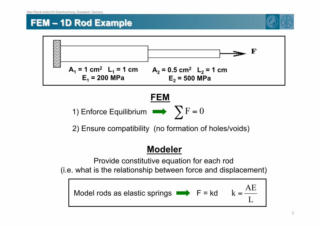
6
2) Ensure compatibility (no formation of holes/voids)
FEM
A1 = 1 cm2 L1 = 1 cm
E1 = 200 MPa A2 = 0.5 cm2 L2 = 1 cm
E2 = 500 MPa
1) Enforce Equilibrium
Modeler
Provide constitutive equation for each rod
(i.e. what is the relationship between force and displacement)
Model rods as elastic springs F = kd

Max-Planck-Institut für Eisenforschung, Düsseldorf, Germany
7
For each element, write a force balance at each node
F
Node 1 Node 2 Node 3
Element 1 Element 2
k1 k2
Element 1 Element 2

Max-Planck-Institut für Eisenforschung, Düsseldorf, Germany
8
!! Apply Boundary Conditions
3 equations and 3 unknowns Easily solve with a matrix inversion
!! Assemble the force balance equations for all 3 nodes
K = Stiffness Matrix u = displacement vector f = force vector
Max-Planck-Institut für Eisenforschung, Düsseldorf, Germany
9
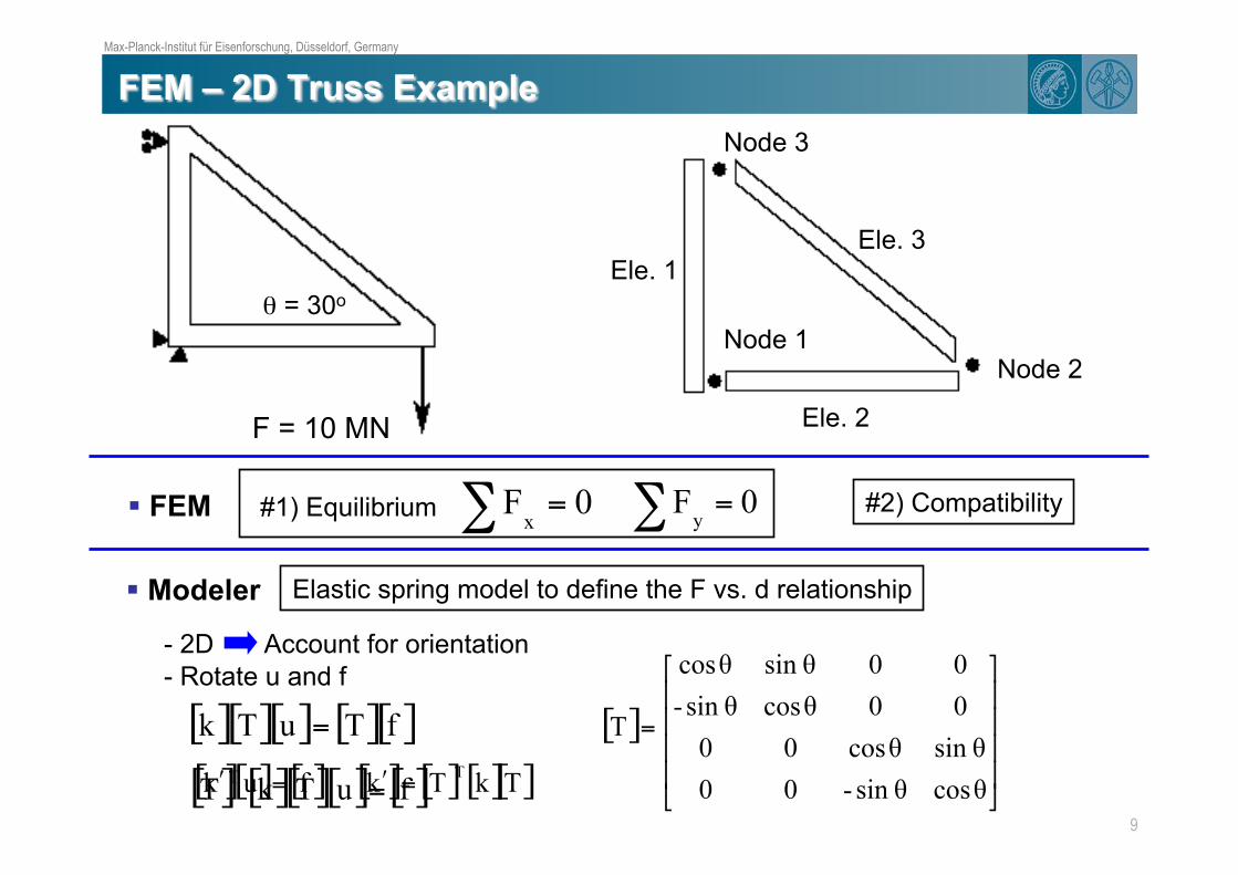
F = 10 MN
" = 30o
Ele. 1
Ele. 2
Ele. 3
Node 1 Node 2
Node 3
!! FEM
!! Modeler
-! 2D Account for orientation
-! Rotate u and f
#1) Equilibrium #2) Compatibility
Elastic spring model to define the F vs. d relationship
Max-Planck-Institut für Eisenforschung, Düsseldorf, Germany
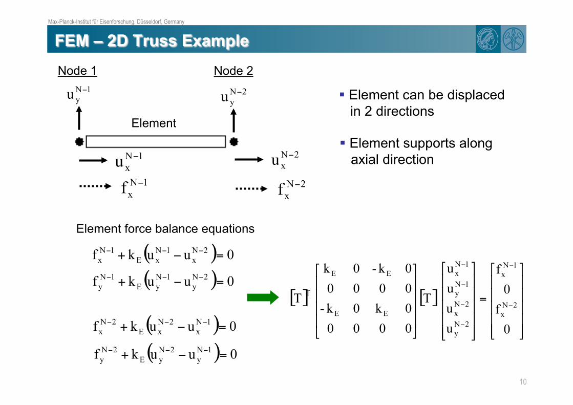
10
Element force balance equations
!! Element supports along
axial direction
Element
Node 1 Node 2
!! Element can be displaced
in 2 directions

Max-Planck-Institut für Eisenforschung, Düsseldorf, Germany
11
A(m2) E(MPa) L(m)
Ele 1 0.01 10 5 Ele 2 0.01 10 8.66
Ele 3 0.01 10 10
Ele. 1
Ele. 2
Ele. 3
Node 1 Node 2
Node 3
k1 = 2000 k2 = 1154.73 k3 = 1000

Max-Planck-Institut für Eisenforschung, Düsseldorf, Germany
12
!! Calculate the element stiffness matrixes
For example Element 3:
Max-Planck-Institut für Eisenforschung, Düsseldorf, Germany
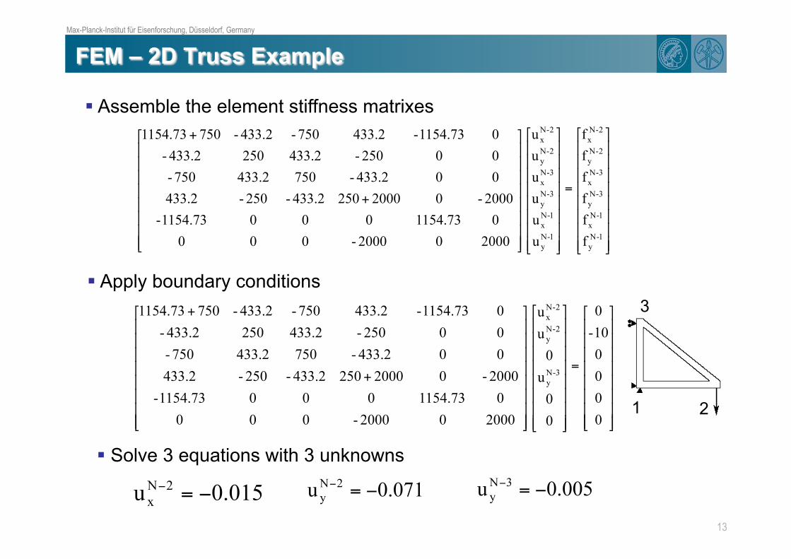
13
!! Assemble the element stiffness matrixes
!! Apply boundary conditions
!! Solve 3 equations with 3 unknowns
1 2
3

Max-Planck-Institut für Eisenforschung, Düsseldorf, Germany
14
!! Governing equations are usually complex differential
equations
!! Often these equations cannot be solved over an element
PROBLEM
Equations do not permit the exact solution
SOLUTION
Instead of finding an exact solution at every point, we find a
solution that satisfies the strong form on average over the
domain
TOOL
Variational Approach

Max-Planck-Institut für Eisenforschung, Düsseldorf, Germany
15
Assume Linear Elastic material:
Weak Form is based on Potential Energy (#)
L
Example System: b
(eng. density)

Max-Planck-Institut für Eisenforschung, Düsseldorf, Germany
16
!! Governing PDE’s with
boundary conditions
L
Strong Form
PDE:
BC:
FEM
Weak Form
!! Variational statement
of the problem
b

Max-Planck-Institut für Eisenforschung, Düsseldorf, Germany
17
Exact solution, u(x) is unknown
FEM “guesses” an admissible displacement field, w(x)
Exact solution for the
displacement field u(x)
Any other “admissible”
displacement field w(x)
L 0 x
Admissible: 1)! 1st derivative must be real
2)! w(0) = 0 (Force BC automatically satisfied)
FEM works w(x)

Max-Planck-Institut für Eisenforschung, Düsseldorf, Germany
18
How are w(x) and u(x) related?
Principle of Minimum Potential Energy
Among all admissible displacements ( w(x)’s ),
the one that MINIMIZES the total potential energy (#) is u(x)
Given the Principle of
Minimum Potential Energy
Iterative scheme to find a w(x)
that closely approximates u(x)
Guess w(x) Calculate #(w) Check accuracy
Unacceptable
Acceptable
FEM
Max-Planck-Institut für Eisenforschung, Düsseldorf, Germany
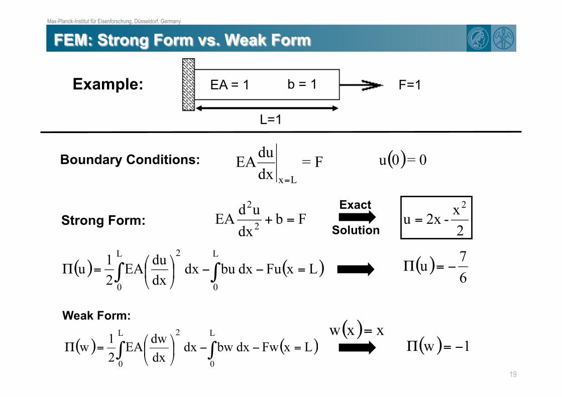
19
L=1
EA = 1 F=1 Example:
Strong Form:
b = 1
Boundary Conditions:
Exact
Weak Form:
Solution

Max-Planck-Institut für Eisenforschung, Düsseldorf, Germany
20
!! Weak Form weaker statement of the problem !! Based on potential energy
!! Has the effect of relaxing the problem
!! “Average” solution over the domain
!! A solution of the strong form will also satisfy the weak
form, but not vice versa.
!! Principle of Minimum Potential Energy !! w(x) that minimizes #, equals u(x)
Strong Form vs. Weak Form

Max-Planck-Institut für Eisenforschung, Düsseldorf, Germany
21
How does FEM determine w(x) function?
w(x) must be 1st order continuous and satisfy BC
Generally, polynomials and sine/cosine functions are simple
enough to be practical.
wi’s are to be determined
Numerical Methodology used to
determine wi’s
Galerkin’s Method/
Rayleigh-Ritz
Max-Planck-Institut für Eisenforschung, Düsseldorf, Germany
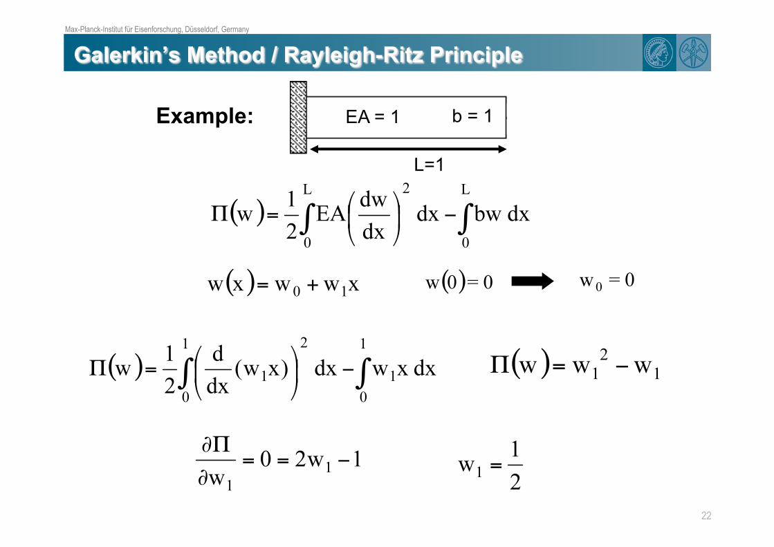
22
L=1
EA = 1 Example: b = 1

Max-Planck-Institut für Eisenforschung, Düsseldorf, Germany
23
At the end points, we get the
exact solution!
Max-Planck-Institut für Eisenforschung, Düsseldorf, Germany
24
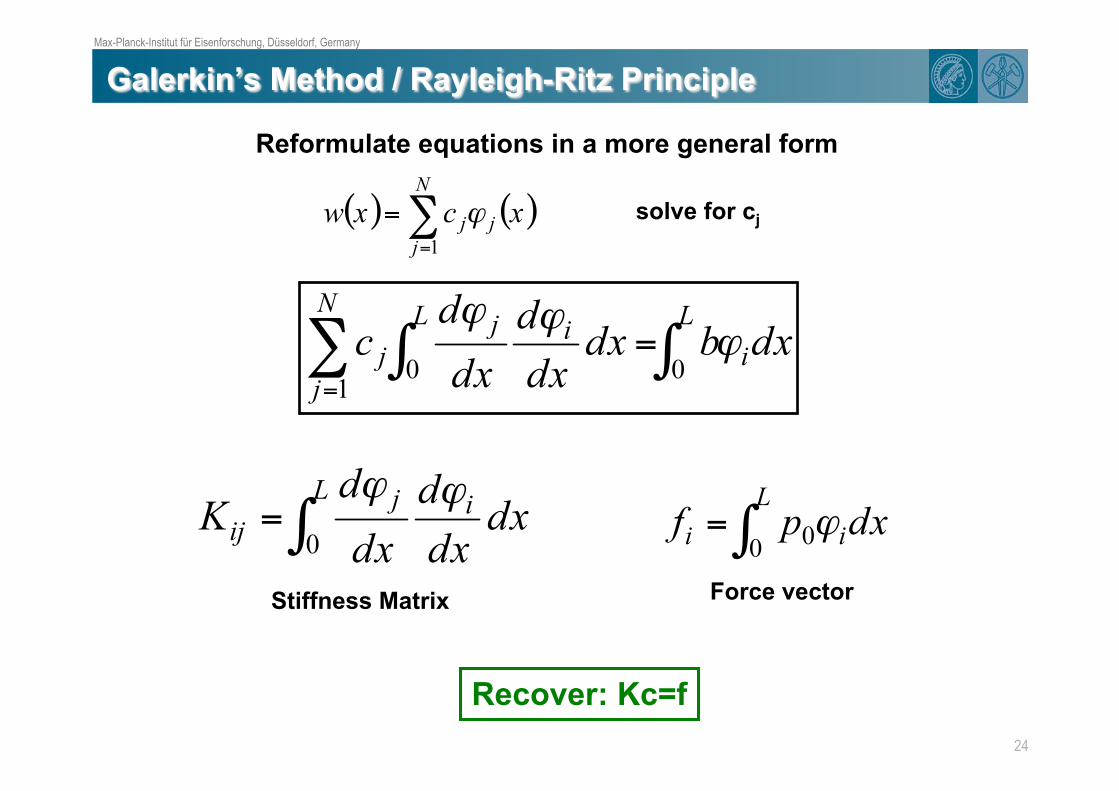
Reformulate equations in a more general form
Recover: Kc=f
solve for cj
Stiffness Matrix Force vector

Max-Planck-Institut für Eisenforschung, Düsseldorf, Germany
25
!! Wide range of element types and shapes
Sample Elements
!! Main difference Solution form within the element
Max-Planck-Institut für Eisenforschung, Düsseldorf, Germany
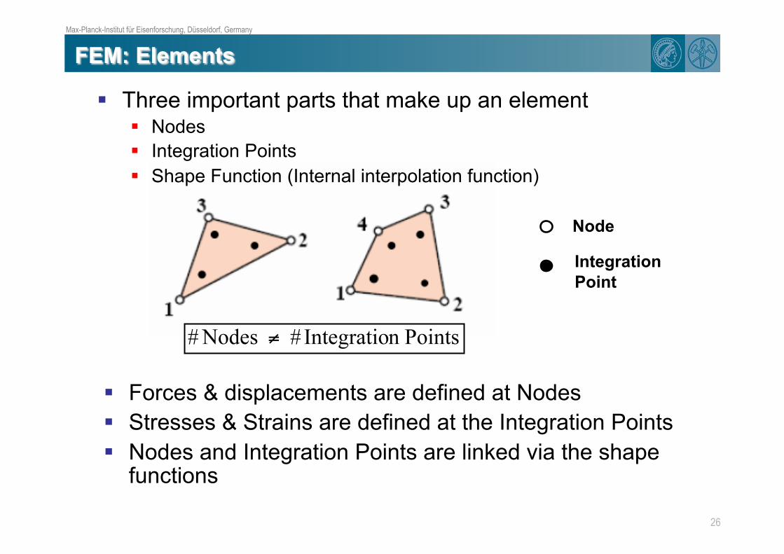
26
Node
Integration
Point
!! Three important parts that make up an element !! Nodes
!! Integration Points
!! Shape Function (Internal interpolation function)
!! Forces & displacements are defined at Nodes
!! Stresses & Strains are defined at the Integration Points
!! Nodes and Integration Points are linked via the shape functions
Max-Planck-Institut für Eisenforschung, Düsseldorf, Germany
27
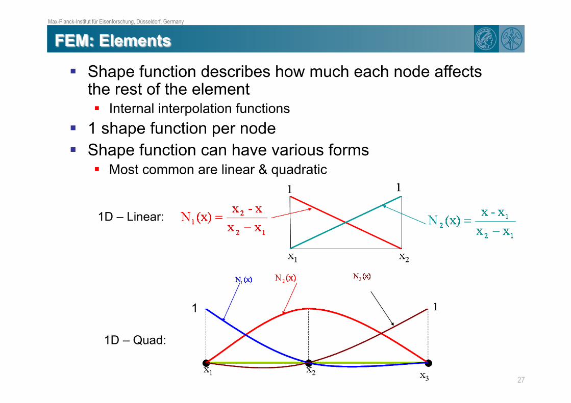
!! Shape function describes how much each node affects the rest of the element !! Internal interpolation functions
!! 1 shape function per node
!! Shape function can have various forms !! Most common are linear & quadratic
1D – Linear:
1D – Quad:
1

Max-Planck-Institut für Eisenforschung, Düsseldorf, Germany
28
Linear Shape functions Quad. Shape Functions
!! 2D Shape functions are planes rather than lines
!! Shape functions guarantee nodal based quantities (like force and displacement) are CONTINUOUS across element boundaries
!! Shape function derivatives are NOT CONTINUOUS across element boundaries
N1 N2 N3
= nodal values

Max-Planck-Institut für Eisenforschung, Düsseldorf, Germany
29
2D Linear Element:
A displacement approximation
v = displacement in y
u = displacement in x

Max-Planck-Institut für Eisenforschung, Düsseldorf, Germany
30
FEM calculates strain from the nodal displacements
Definition of Strain FEM Strain Calculation
Based on the derivative of the shape functions
!! Because shape function derivatives are NOT CONTINUOUS across
element boundaries, calculating $ at nodes could be a problem.
!! $ is always calculated at integration points (inside the element)

Max-Planck-Institut für Eisenforschung, Düsseldorf, Germany
31
Linear Shape Functions
Linear shape functions lead to elements that have a
constant strain profile
Note: No dependence on x
1D Element with Linear Shape Functions
x1 x2
L
Define a shape function derivative matrix: [B]

Max-Planck-Institut für Eisenforschung, Düsseldorf, Germany
32
Quadratic shape functions lead to elements that have
a linear strain profile
Note: There is linear dependence on x
Quad. Shape Functions
1D Element with Quadratic Shape Functions
x1 x2
L
x3

Max-Planck-Institut für Eisenforschung, Düsseldorf, Germany
33
Linear shape functions lead to elements that have a
constant strain profile
Linear Shape Functions
Note: No dependence on x and y
Max-Planck-Institut für Eisenforschung, Düsseldorf, Germany
34
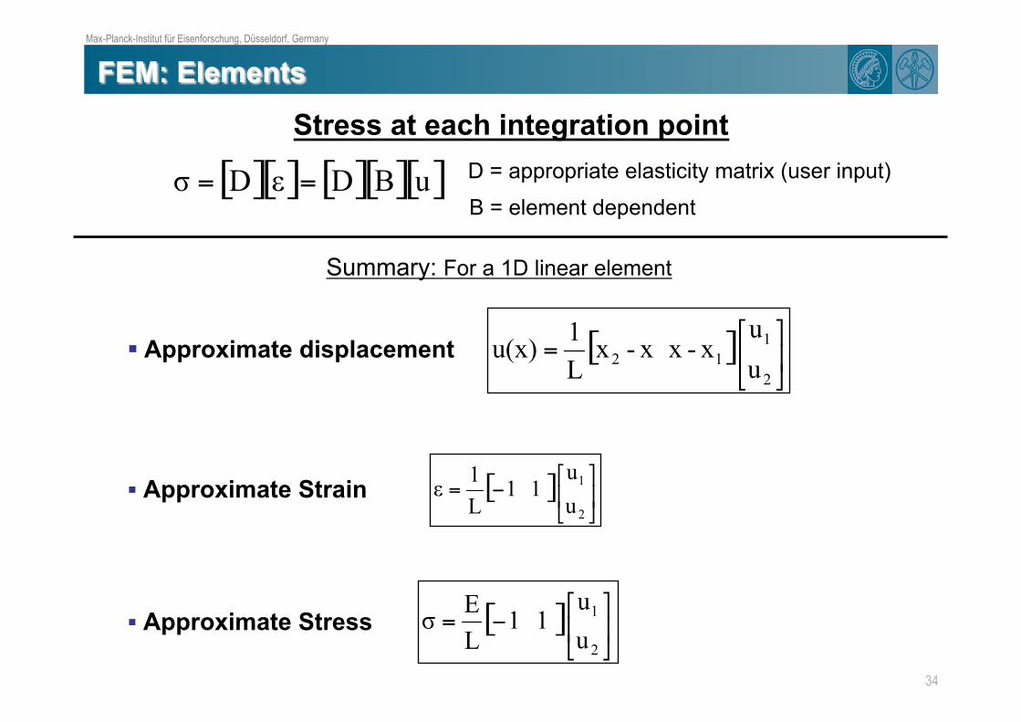
Stress at each integration point
D = appropriate elasticity matrix (user input)
B = element dependent
!! Approximate displacement
!! Approximate Strain
Summary: For a 1D linear element
!! Approximate Stress

Max-Planck-Institut für Eisenforschung, Düsseldorf, Germany
35
!! Assemble individual element stiffness matrix
FEM Method with Elements
!! Apply Boundary Conditions
!! Assemble global stiffness matrix

Max-Planck-Institut für Eisenforschung, Düsseldorf, Germany
36
There are three general sources of error in
a finite-element solution
#1: Errors due to the approximation of the domain
#2: Errors due to the approximation of the solution
#3: Errors due to numerical computation
(like numerical integration and round-off errors in a computer)
The estimation of these errors, in general, is not
a simple matter.
vs.
vs.

Max-Planck-Institut für Eisenforschung, Düsseldorf, Germany
37
!! The accuracy and convergence of the finite-element solution depends on a number of factors
!! Like the differential equation solved (or the variational form used) and the type of element.
!! Accuracy
!! Difference between the exact
solution and the finite-element
solution
!! Convergence
!! The accuracy of the solution
as the number of elements in
the mesh is increased
Converged solution is NOT necessarily an accurate solution Desired Result

Max-Planck-Institut für Eisenforschung, Düsseldorf, Germany
38
!! FEM Partial Differential Equation Solver
!! Solves PDE by
1)! Breaking solution space into pieces (elements)
2)! Approximating the solution on each element
3)! Solving a force balance (equilibrium) equation
K = stiffness matrix (composed of element and material
properties)
!! FEM solves the weak form of the equilibrium equation
!! “Average” solution over the domain NOT the exact solution
!! Three primary parts of an element
!! Nodes
!! Integration Points
!! Shape Functions

Max-Planck-Institut für Eisenforschung, Düsseldorf, Germany
39
!! Large number of element types and shapes
!! Element choice will affect your results
!! FEM Error
!! Domain Approximation
!! Solution Approximation
!! Numerical Computations
!! Convergence vs. Accuracy
!! A converged result is NOT necessarily an accurate result
Linear elements Constant strain
Quadratic elements Linear strain
Any physically meaningful output MUST result from physical
input provided by you to FEM
FEM error is difficult to quantify

Max-Planck-Institut für Eisenforschung, Düsseldorf, Germany
40
Examples:
Coupled temperature and
deformation problems
Time dependent temperature
analysis due to friction

Max-Planck-Institut für Eisenforschung, Düsseldorf, Germany
41
Complex deformations Elastic spring-back

Max-Planck-Institut für Eisenforschung, Düsseldorf, Germany
42
Multiple components/complex geometries

Max-Planck-Institut für Eisenforschung, Düsseldorf, Germany
43
•! 2 Material Science examples
–! FEM “works”
!!Converges to a solution
!!Solution is not correct
•! Length scale issues
•! Inhomogeneous Materials

Max-Planck-Institut für Eisenforschung, Düsseldorf, Germany
44
150 um! 3.4 um!!! Finite element mesh
has dimensions!
!! Structural finite
element codes are
continuum based!
!! Predicted %!$ results
from two different
grain sizes are similar!
!! Local models:
dimensions do not
effect the %!$ result!

Max-Planck-Institut für Eisenforschung, Düsseldorf, Germany
45
Problem Statement
To investigate the effect of element type and mesh
resolution on the %-$ response of a two phase material.
(Hard Phase: Martensite) (Soft Phase: Ferrite)
Motivation
!! Accounting for microstructure heterogeneity within a
material computationally expensive.
!! At the microscopic scale, strain and stress path are
complex.
!! Generally, it is not possible to exactly mesh and simulate
the material’s microstructure

Max-Planck-Institut für Eisenforschung, Düsseldorf, Germany
46
Coarsest Mesh: 1 Material per Int. Point
12 x 12 elements (144 total elements) 48 x 48 elements (2304 total elements)
Finest Mesh: 1 Material per 4 elements Material
per IP
Material
per element
Material
per 4 elements

Max-Planck-Institut für Eisenforschung, Düsseldorf, Germany
47
•! Element Types
–! 2D Linear (4 nodes)
–! 2D Quadratic (9 nodes)
Full Integration Reduced Integration
Full Integration Reduced Integration

Max-Planck-Institut für Eisenforschung, Düsseldorf, Germany
48
•! Prescribe displacements
•! Volume conserving ($x = $y)
2D Plane Strain Rolling
•! 30 % thickness reduction
•! Elastic-plastic constitutive equations
Study the effect of element type & mesh resolution on the %-$ response

Max-Planck-Institut für Eisenforschung, Düsseldorf, Germany
49
Element type and mesh resolution do
affect the overall %-$ response
&%Total =100 MPa
%-$ curves of 4 different element types with 3 different mesh resolutions
&%Linear = 10 MPa
&%Quad = 70 MPa

Max-Planck-Institut für Eisenforschung, Düsseldorf, Germany
50
Increasing the mesh resolution leads to a softer %-$ response
Element type: Quadratic; Full integration
&% = 45 MPa

Max-Planck-Institut für Eisenforschung, Düsseldorf, Germany
51
Use of quad. elements leads to a softer response.
Use of reduced integration leads to a harder
response.
Mesh resolution

Max-Planck-Institut für Eisenforschung, Düsseldorf, Germany
52
!! Linear elements $ is relatively flat
!! Quad elements $ flows around the martensite
Quad Element; Full Integration Linear Element; Full Integration
Mesh resolution
Strain state appears reasonable

Max-Planck-Institut für Eisenforschung, Düsseldorf, Germany
53 Use of linear elements GREATLY reduces computation time

Max-Planck-Institut für Eisenforschung, Düsseldorf, Germany
54
!! Mesh dimensions do not enter into %-$ constitutive relationship
!! Element type and mesh resolution do affect the overall %-$ response !! &% = 100 MPa
!! Increasing the mesh resolution leads to a softer %-$ response
!! Use of quadratic elements leads to a softer %-$ response
!! Linear elements predict a relatively flat e profile
!! Quadratic elements predict a much more contoured e profile
!! Use of linear elements GREATLY reduces computation time
content
PART IV
Polycrystal Plasticity Models

micro-macro homogenization
motivation
material point comprises lots of grains
representation of texture
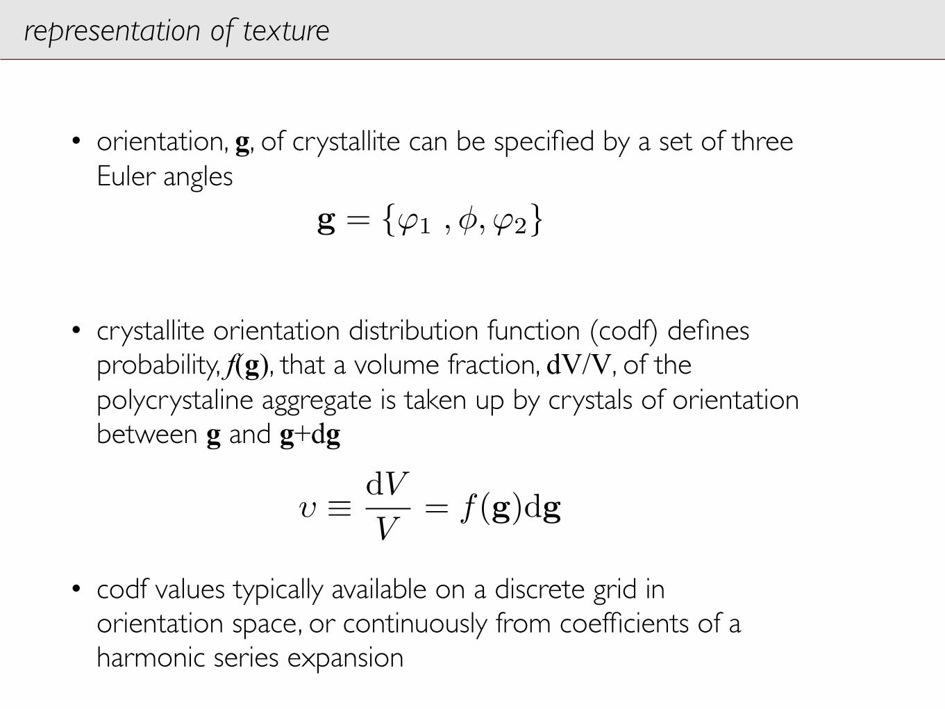
• orientation, g, of crystallite can be specified by a set of three Euler angles
• crystallite orientation distribution function (codf) defines probability, f(g), that a volume fraction, dV/V, of the polycrystaline aggregate is taken up by crystals of orientation between g and g+dg
• codf values typically available on a discrete grid in orientation space, or continuously from coefficients of a harmonic series expansion
υ ≡ dV
V= f(g)dg
g = {ϕ1 , φ,ϕ2}

goal
!box spacing
orientation
i-1 i i+1

goal
!box spacing
orientation
i-1 i i+1
• select N * from all those N orientations having non-zero !i in discrete
codf representation

probabilistic reconstruction
!box spacing
orientation
i-1 i i+1

• add randomly selected orientation if random number
• continue until N * orientations collected
probabilistic reconstruction
r ∈ [0, 1] ≤ υi
L.S. Tóth, P. Van Houtte, Textures Microstruct. 19 (1992) 229–244.
!box spacing
orientation
i-1 i i+1

• add randomly selected orientation if random number
• continue until N * orientations collected
probabilistic reconstruction
!
orientation
r ∈ [0, 1] ≤ υi
L.S. Tóth, P. Van Houtte, Textures Microstruct. 19 (1992) 229–244.

• add randomly selected orientation if random number
• continue until N * orientations collected
probabilistic reconstruction
!
orientation
r ∈ [0, 1] ≤ υi
L.S. Tóth, P. Van Houtte, Textures Microstruct. 19 (1992) 229–244.

• add randomly selected orientation if random number
• continue until N * orientations collected
probabilistic reconstruction
!
orientation
r ∈ [0, 1] ≤ υi
L.S. Tóth, P. Van Houtte, Textures Microstruct. 19 (1992) 229–244.
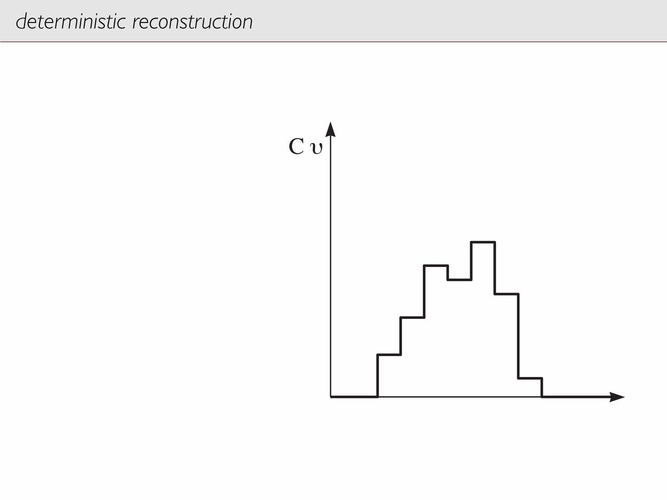
deterministic reconstruction
C !

• select each orientation
times
deterministic reconstruction
1
0.5
C !
n* = 0 0 1 1 0 01
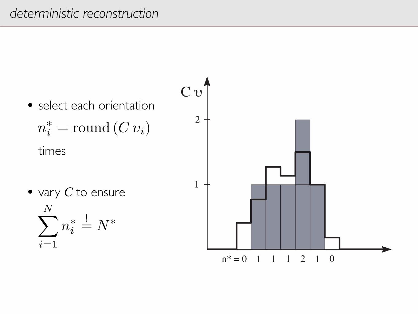
n∗i = round (C υi)

• select each orientation
times
• vary C to ensure
deterministic reconstruction
1
0.5
C !
n* = 0 0 1 1 0 01
N∑
i=1
n∗i
!= N∗
n∗i = round (C υi)
• select each orientation
times
• vary C to ensure
deterministic reconstruction
2
1
n* = 0 1 1 2 1 01
C !
N∑
i=1
n∗i
!= N∗
n∗i = round (C υi)

• select each orientation
times
• vary C to ensure
deterministic reconstruction
1
2
3
n* = 1 2 3 3 2 03
C !
N∑
i=1
n∗i
!= N∗
n∗i = round (C υi)
T. Leffers, D. Juul Jensen, Textures Microstruct. 6 (1986) 231–263.
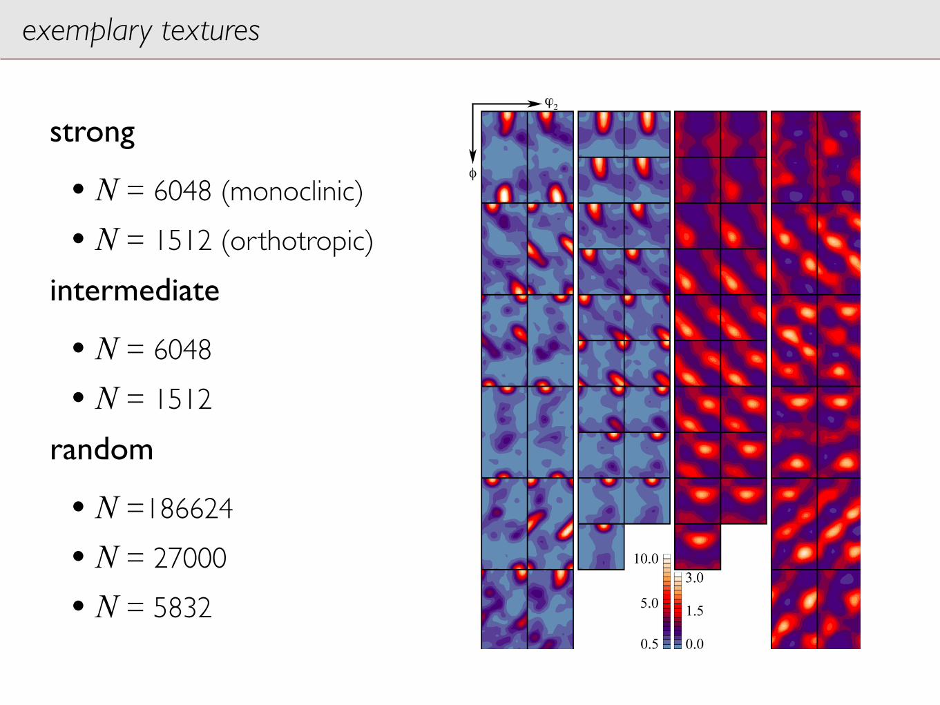
exemplary textures
strong
• N = 6048 (monoclinic)
• N = 1512 (orthotropic)
intermediate
• N = 6048
• N = 1512
random
• N =186624
• N = 27000
• N = 5832

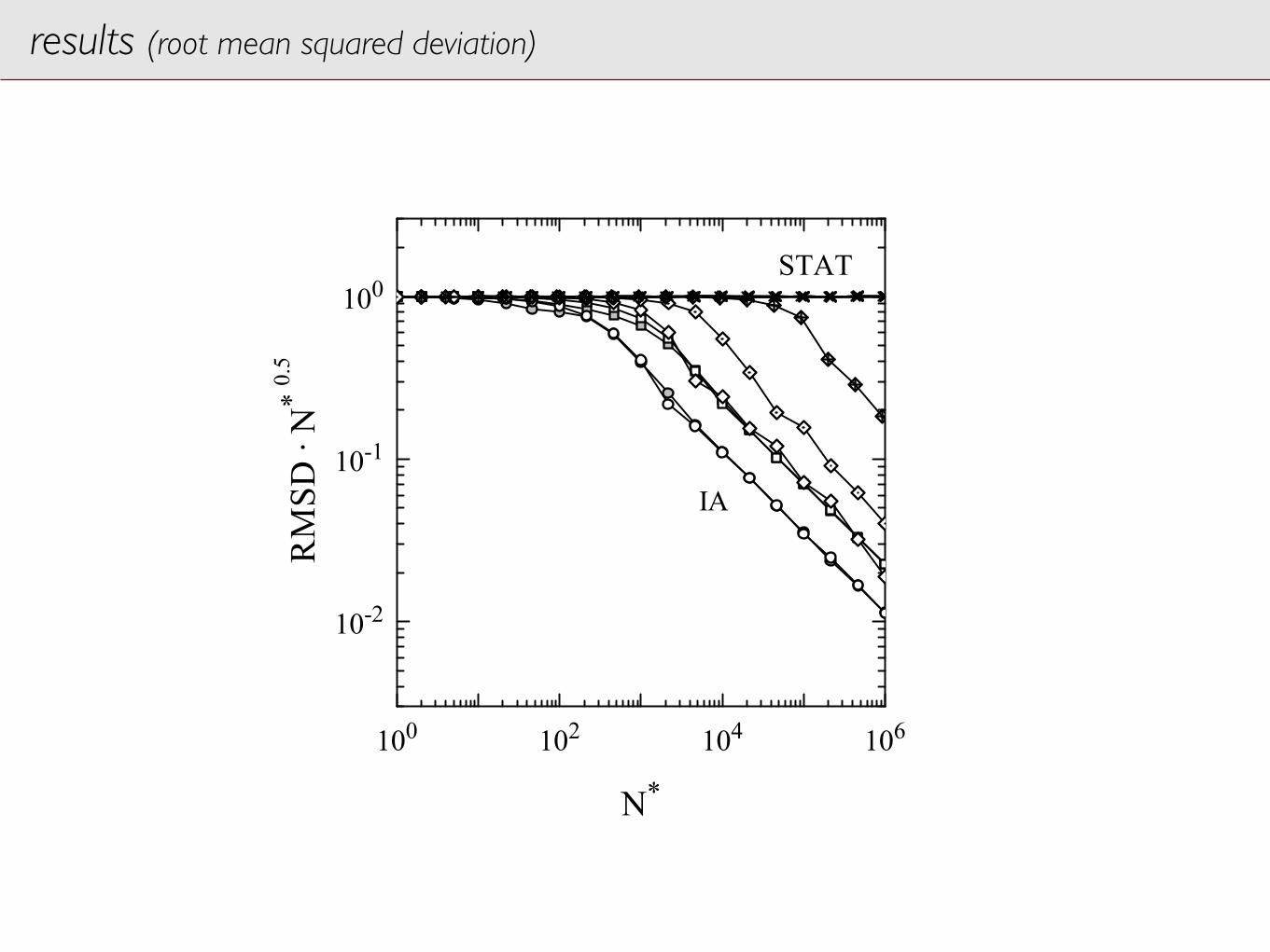
measure of approximation quality
RMSD =
√√√√N∑
i=1
(υi − υ∗i )2

100
102
104
106
10-6
10-4
10-2
100
STAT
IA
RM
SD
N*
results (root mean squared deviation)
100
102
104
106
10-2
10-1
100
IA
STAT
!
"#$%
!&!'(!)*+
N*
results (root mean squared deviation)

10-4
10-2
100
102
10-2
10-1
100
!
"#$%
!&!'(!)*+
N*/N
STAT
IA
results (root mean squared deviation)
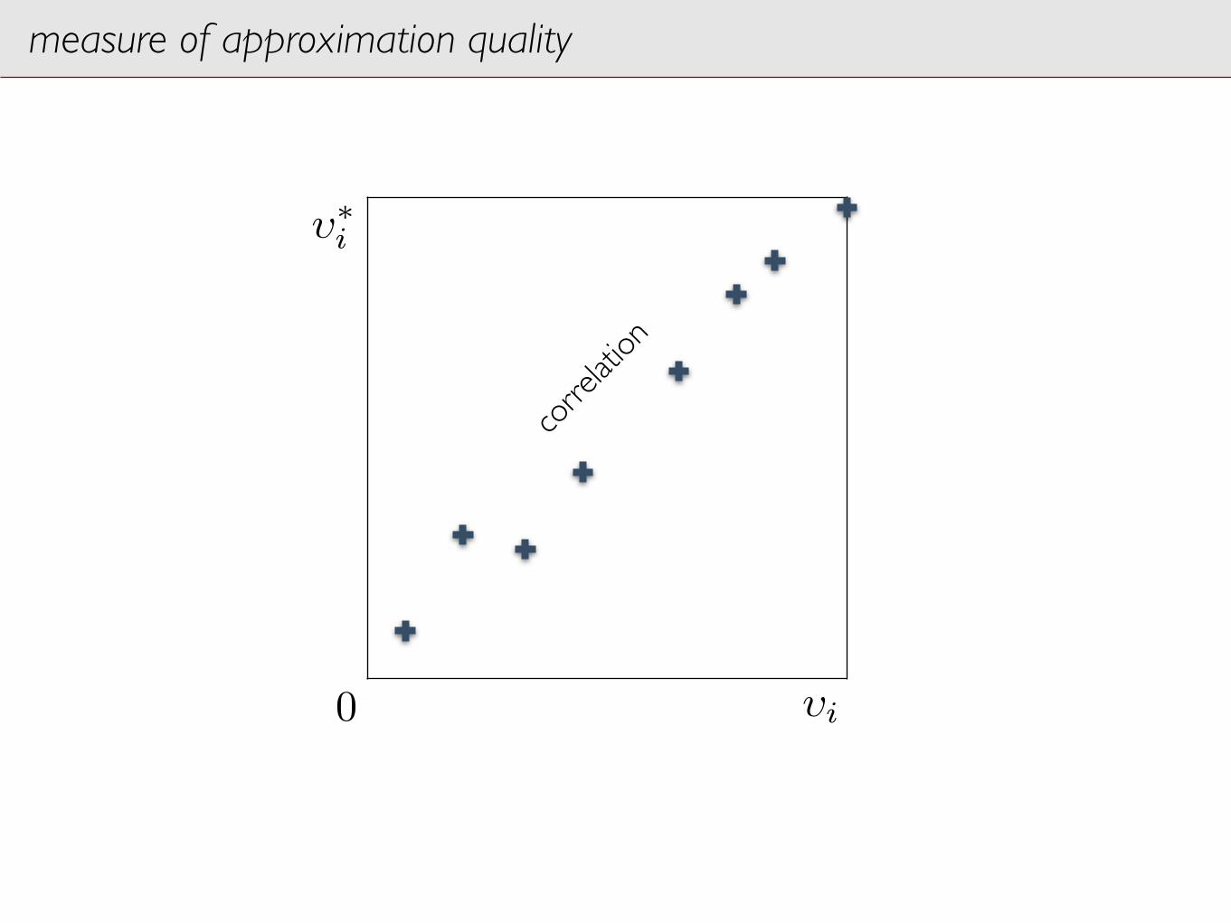
measure of approximation quality
υi
υ∗i
0
corre
lation

a
fC
measure of approximation quality
a =N
N∑i=1
υiυ∗i −N∑
i=1υi
N∑i=1
υ∗i
NN∑
i=1υiυi −
N∑i=1
υi
N∑i=1
υi
fC =
N∑i=1
υiυ∗i /N −⟨υi
⟩⟨υ∗i
⟩
√⟨υi
2⟩−
⟨υi
⟩2√⟨
υ∗i2⟩−
⟨υ∗i
⟩2
J. Tarasiuk and K. Wierzbanowski, Phil. Mag. A 73 (1996) 1083–1091
υi
υ∗i
0
corre
lation

results (correlation for strong texture / probabilistic reconstruction)
0 0.5
0.0
0.5
1.0
1.5
2.0
0 0.5 0 0.5 1
!
* i /
%N
*/N = 1/8 1/2 2
!i / %
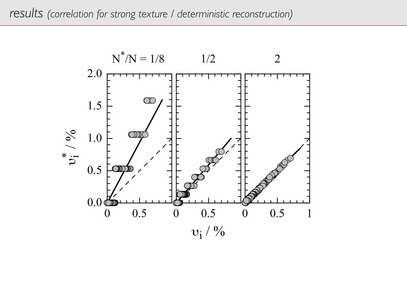
results (correlation for strong texture / deterministic reconstruction)
0 0.5
0.0
0.5
1.0
1.5
2.0
0 0.5 0 0.5 1
!* i /
%1/2 2N
*/N = 1/8
!i / %

10-4
10-2
100
102
0.1
0.2
0.4
0.6
0.8
1
f C
N*/N
IA STAT
results (correlation factor)

10-4
10-2
100
102
0.1
0.2
0.4
0.6
0.8
1
IA STAT
f C
N*/N
results (correlation factor)

10-4
10-2
100
102
0.1
0.2
0.4
0.6
0.8
1
IA STAT
f C
N*/N
results (correlation factor)

10-4
10-2
100
102
0
2
4
a
N*/N
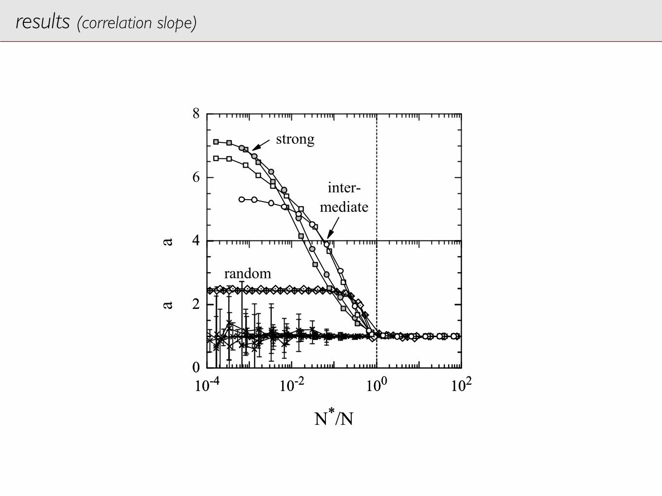
results (correlation slope)
10-4
10-2
100
102
0
2
4
a
N*/N
10-4
10-2
100
102
0
2
4
6
8
inter-
mediate
a
N*/N
strong
random
results (correlation slope)

10-4
10-2
100
102
0
2
4
a
N*/N
10-4
10-2
100
102
0
2
4
6
8
inter-
mediate
a
N*/N
strong
random
results (correlation slope)
1
0.5
C !
n* = 0 0 1 1 0 01
1
2
3
n* = 1 2 3 3 2 03
C !
N∑
i=1
n∗i
!= max (N∗, N)
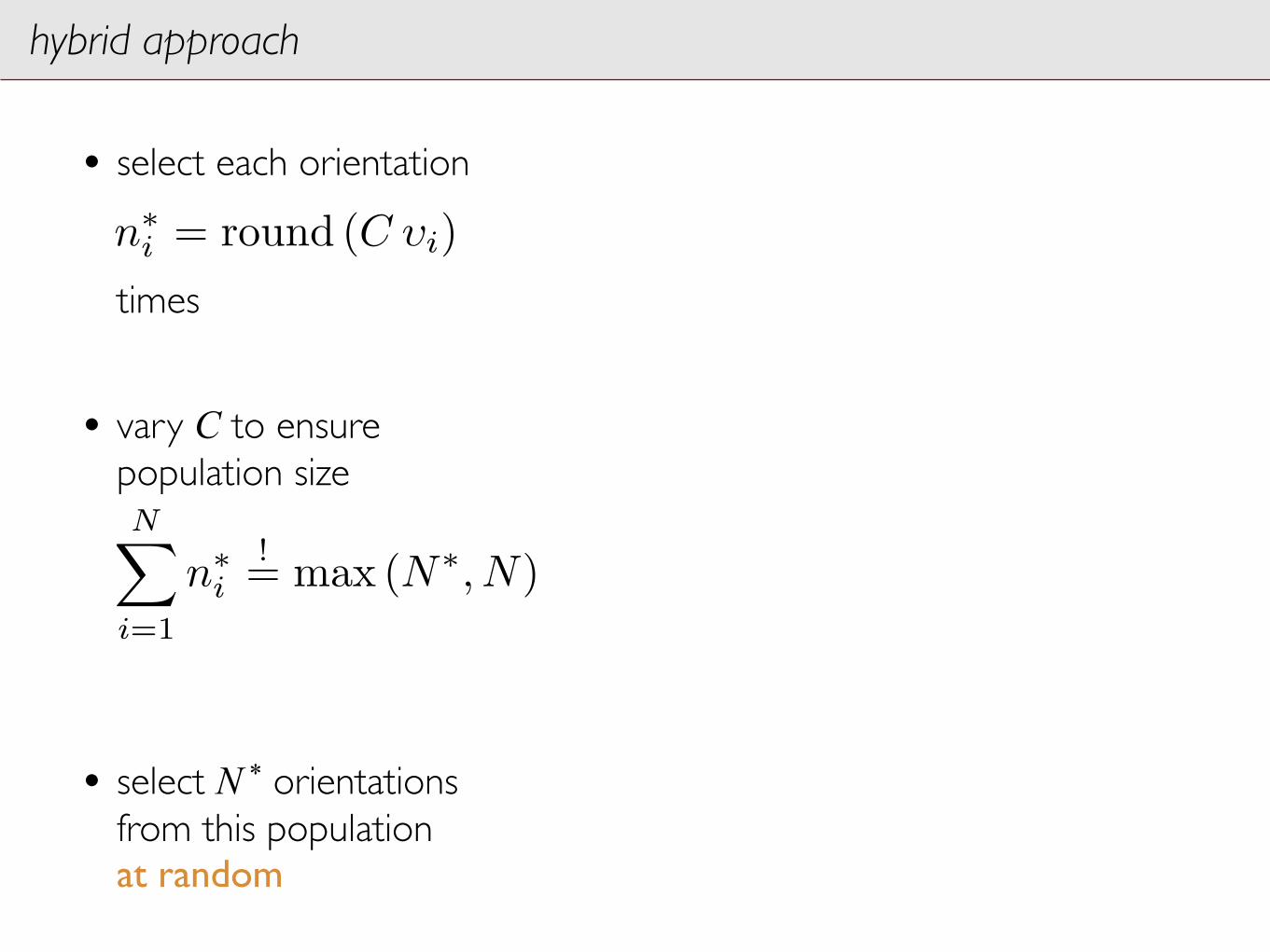
hybrid approach
• select each orientation
times
• vary C to ensure population size
• select N * orientations from this population at random
n∗i = round (C υi)

2
1
n* = 0 1 2 2 1 01
C !
N∑
i=1
n∗i
!= max (N∗, N)
hybrid approach
• select each orientation
times
• vary C to ensure population size
• select N * orientations from this population at random
n∗i = round (C υi)

N∑
i=1
n∗i
!= max (N∗, N)
hybrid approach
• select each orientation
times
• vary C to ensure population size
• select N * orientations from this population at random
n∗i = round (C υi)
2
1
n* = 0 1 2 2 1 01
C !
0 0.5
0.0
0.5
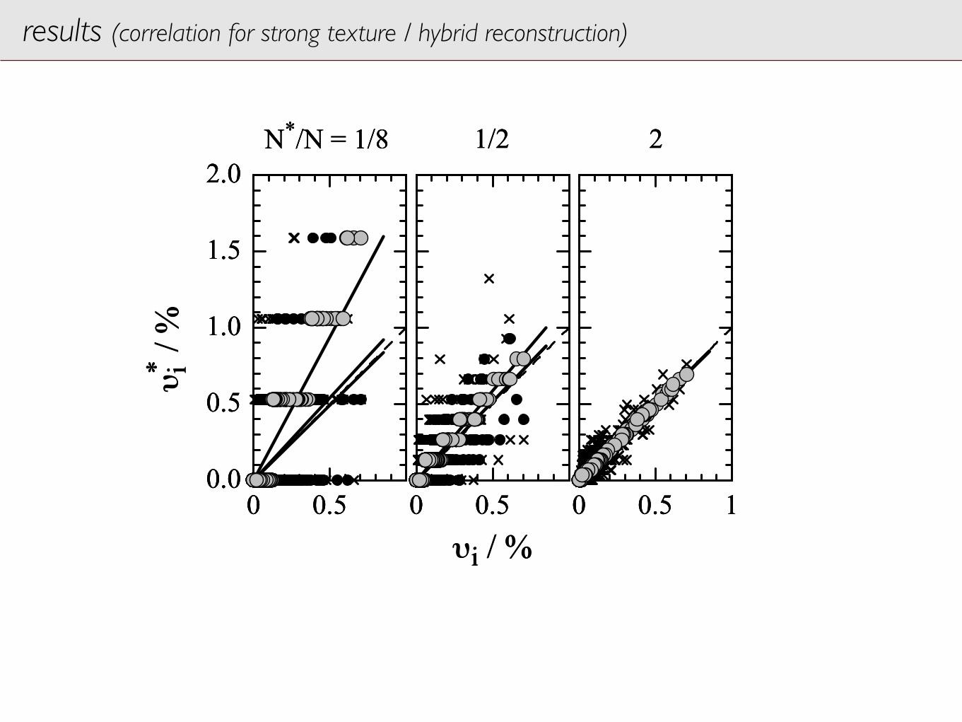
1.0
1.5
2.0
0 0.5 0 0.5 1
N*/N = 1/8 1/2 2
!* i /
%
!i / %
0 0.5
0.0
0.5
1.0
1.5
2.0
0 0.5 0 0.5 1
!
* i /
%N
*/N = 1/8 1/2 2
!i / %
0 0.5
0.0
0.5
1.0
1.5
2.0
0 0.5 0 0.5 1
!* i /
%1/2 2N
*/N = 1/8
!i / %
results (correlation for strong texture / hybrid reconstruction)

results (correlation factor)
10-4
10-2
100
102
0.1
0.2
0.4
0.6
0.8
1
10-4
10-2
100
102
10-4
10-2
100
102
IA
f C
!
hybrid IA
STAT STAT
hybrid IA
IA
"
N*/N
STAT
IA
random
10-4
10-2
100
102
0
2
4
a
N*/N
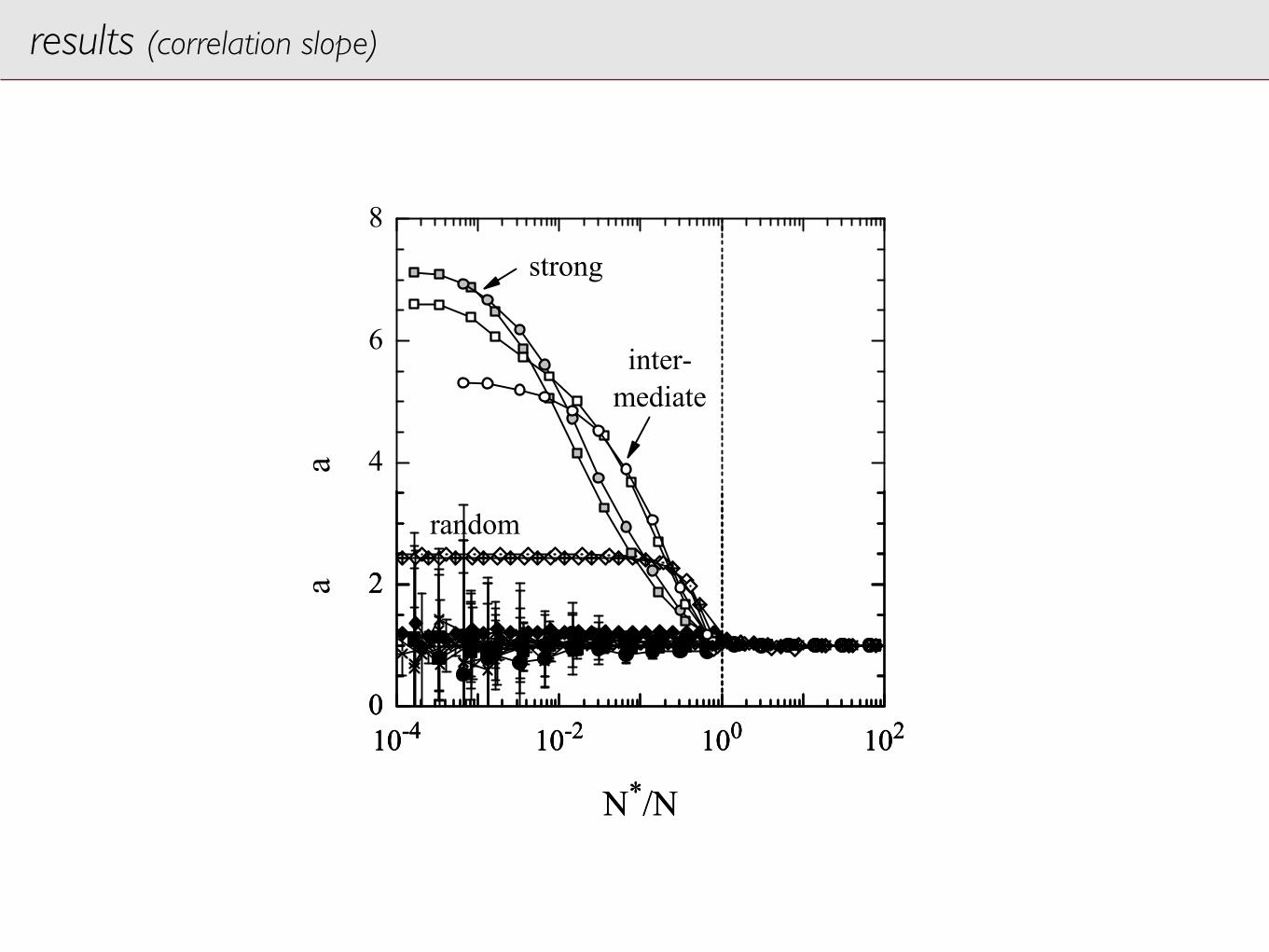
results (correlation slope)
10-4
10-2
100
102
0
2
4
6
8
inter-
mediate
a
N*/N
strong
random
10-4
10-2
100
102
0
2

results (root mean squared deviation)
10-4
10-2
100
102
10-2
10-1
100
!
"#$%
!&!'(!)*+
N*/N
10-4
10-2
100
102
10-2
10-1
100"#$%
!&!'(!)*+
N*/N
STAT
IA
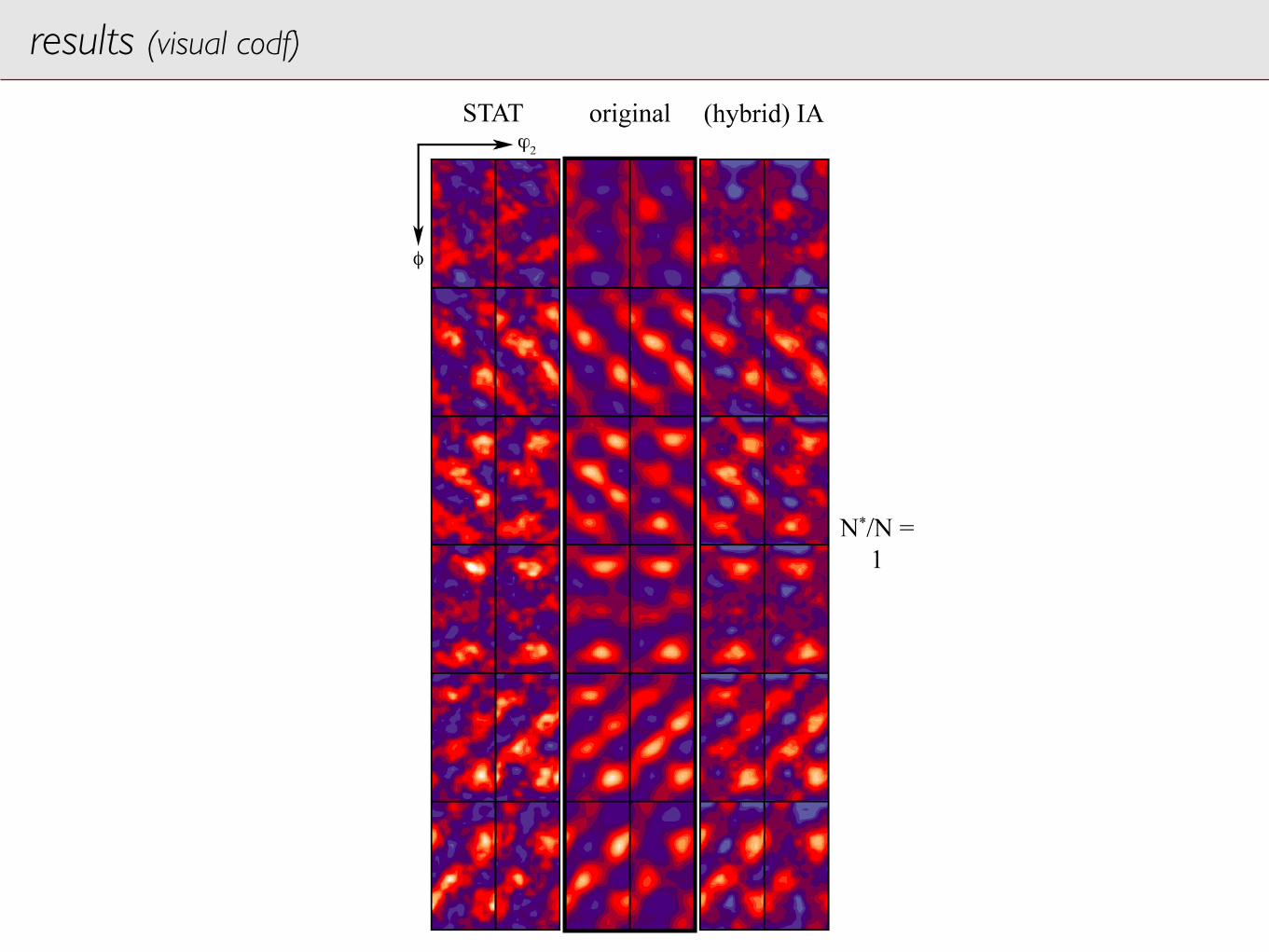
results (visual codf)