FEEM’S INPUT TO CliMares Arctic WP 310 NERSC, BERGEN, 22-23 October 2009 Andrea Bigano.
30
FEEM’S INPUT TO CliMares Arctic WP 310 NERSC, BERGEN, 22-23 October 2009 Andrea Bigano
-
Upload
colin-booth -
Category
Documents
-
view
214 -
download
0
Transcript of FEEM’S INPUT TO CliMares Arctic WP 310 NERSC, BERGEN, 22-23 October 2009 Andrea Bigano.

FEEM’S INPUT TO CliMares Arctic WP 310
NERSC, BERGEN, 22-23 October 2009
Andrea Bigano

CliMares Arctic2
WP310: Economic impact studies
WP310 in particular is the one in which FEEM models can be applied. It is however crucial to understand how these models can interact with the model already proposed (i.e. MADIAMS-ARCTIC modelling tool)
The ICES model can be useful to unravel the economic interconnections among the sectors analysed in the other WP within a computable general equilibrium (CGE) model.
The WITCH model could instead be used to assess the effect of the positive feedback effects of climate change on the Arctic on mitigation policies and costs (albedo reduction , CH4 release from permafrost thawing etc. on the basis of the physical impact assessment results of other WPs. This issue seems very relevant to us, but not touched in the current version of the proposal at least after a very quick view of the document.
In theory we believe that, according to what we know already of the MADIAMS model, there should be an innovative stream of research open and to be explored in this project in which we should work on the coupling of multiscale models from top-down CGE models to bottom-up agent based models, with MADIAMS, somehow in the middle, with the capability of taking advantage of large scale signals provided by the FEEM models cited above and integrate also those coming from bottom-up approaches, such as the approach of the paper by Berman et al., attached to this.
CliMares Arctic3
WITCH
The use of Integrated Assessment Modelsfor studying Climate Change
CliMares Arctic4
IAMs
Climate Change is an intrinsically long term problem
Nightmare of any modeler: action taken now affects variables decades or centuries from now
Integrated Assessment Models (IAMs) combine economy-energy-environment
It is then possible to study how these three macro areas interact among themselves and try to assess policies for counteracting climate change
Two broad classes: Top-down (TD): macroeconomic models with little energy detail Bottom-up (BU): energy system models without a proper description of the
macroeconomic environment Hybrid: try to combine the two classes above to grasp a better understanding
CliMares Arctic5
Main features/1
Ramsey-type neo-classical optimal growth (dynamic, perfect foresight)
Detailed energy input specification (BU)
Hard-link (stand-alone optimization) hybrid
World, 12 regions, interacting strategically (open-loop game)
Endogenous Technical Change
Climate module feedback
Solved numerically
WITCH: a “TOP DOWN” optimization framework, with a energy sector description as a downward expansion of the energy input.

CliMares Arctic6
“TOP DOWN “ perspective: strategic optimal investment strategy both on a time dimension (inter-temporality) and a regional dimension (non-cooperative game)
“BOTTOM UP” component: enables a strategic assessment of the optimal investment in different energy technologies
Electric and non electric energy use 6 Fuels types (Oil, Gas, Coal, Uranium, Trad. Biofuels, Adv. Biofuels) 7 Technologies for electricity generation (+ 1 Backstop Technology)
Optimal intertemporal investment strategies in all fuel technologies and R&D are determined as a dynamic Nash equilibrium of the game among the 12 regions (free riding incentives on CO2 , fuel prices, LbD, LbR).
When choosing optimal investments agents are forward looking (take into account future events, including future policies) and behave strategically (take into account present and future policy measures in the other regions).
Main features/2

CliMares Arctic7
Regional Disaggragation/1
World disaggregated into 12 macro regions, clustered on the basis of geography, income and the structure of energy demand.
Each region behaves strategically in a non-cooperative game, interacting through 5 channels:
CO2 externality (climate damage feedback)
Fossil Fuel prices (aggregate demand)
Investment costs of W&S (Learning by Doing)
Price of Advanced Biofuels (work in progress)
Global CO2 permit market (when emission caps are imposed)

CliMares Arctic8
Regional Disaggregation/2
CAJANZ (Canada, Japan, New Zealand)USALACA (Latin America, Mexico and Caribbean)OLDEURO (Old Europe)NEWEURO (New Europe)MENA (Middle East and North Africa)SSA (Sub-Saharan Africa excl. South Africa)TE (Transition Economies)SASIA (South Asia)CHINA (including Taiwan)EASIA (South East Asia)KOSAU (Korea, South Africa, and Australia)

CliMares Arctic9
Output and Climate Damage
Gross output produced via capital, labour (=population) and energy services.
Climate Damage
(3) tntnESntnLtnKntnTFPtnY nnC ,,))(1(,,)(,,
/1)()(1
Climate Module
EmissionsCO2 emissions
CO2 concentrations
Radiative Force
Temperature
CliMares Arctic10
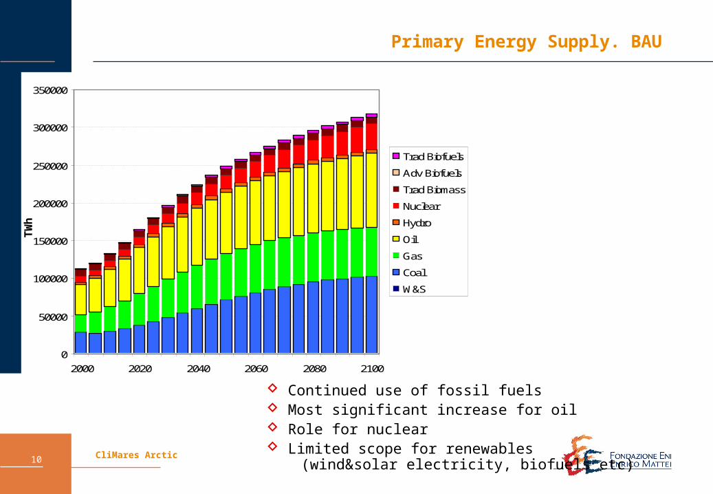
Primary Energy Supply. BAU
0
50000
100000
150000
200000
250000
300000
350000
2000 2020 2040 2060 2080 2100
Trad Biofuels
Adv Biofuels
Trad Biomass
Nuclear
Hydro
Oil
Gas
Coal
W&S
TW
h
Continued use of fossil fuels Most significant increase for oil Role for nuclear Limited scope for renewables (wind&solar electricity, biofuels etc)

CliMares Arctic11
BAU: World Electricity Mix
World Electricity Generation
TW
h
2000 2020 2040 2060 2080 21000
1
2
3
4
5
6x 10
4
BackNuclearHydroelectricOilGasAdv Coal+CCSCoal deSOX deNOXOld CoalWind&Solar
Electricity increases steadily Coal supplies most of the demand Nuclear plays an important role

CliMares Arctic12
Emissions by Region. BAUCO2 Emissions by Region
GtC
2020 2040 2060 2080 21000
5
10
15
20
25
LACAEASIACHINASASIASSAMENATECAJANZKOSAUNEWEUROOLDEUROUSA
20 GtC by 2100Developing Asia the biggest emitter
CliMares Arctic13
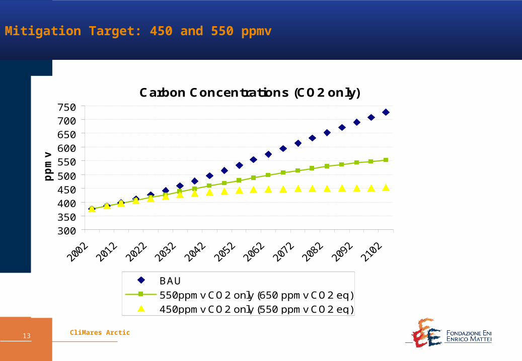
Mitigation Target: 450 and 550 ppmv
Carbon Concentrations (CO2 only)
300350400450500
550600650700750
pp
mv
BAU
550ppmv CO2 only (650 ppmv CO2 eq)
450ppmv CO2 only (550 ppmv CO2 eq)

CliMares Arctic14
Mitigation Target: 450 and 550 ppmv
Radiative Forcing
0
1
2
3
4
5
6
7
W/m
^2
BAU
450ppmv CO2 only (550 ppmv CO2 eq)
550ppmv CO2 only (650 ppmv CO2 eq)

CliMares Arctic15
Trajectories in the energy intensity/carbon intensity wrt 2002
-10%
0%
10%
20%
30%
40%
50%
60%
0% 20% 40% 60% 80%
Reduction in Energy Intensity wrt 2002
Re
du
cti
on
in
Ca
rbo
n
Inte
ns
ity
wrt
20
02
BAU
Trajectories in the energy intensity/carbon intensity wrt 2002
-10%
0%
10%
20%
30%
40%
50%
60%
0% 20% 40% 60% 80%
Reduction in Energy Intensity wrt 2002
Re
du
cti
on
in
Ca
rbo
n
Inte
ns
ity
wrt
20
02
550
BAU
Energy and Carbon Intensities
Trajectories in the energy intensity/carbon intensity wrt 2002
-10%
0%
10%
20%
30%
40%
50%
60%
0% 20% 40% 60% 80% 100%
Reduction in Energy Intensity wrt 2002
Re
du
cti
on
in
Ca
rbo
n
Inte
ns
ity
wrt
20
02
450
550
BAU
2100
2100
2100
Energy efficiency
Dec
arbo
nisa
tion
CliMares Arctic16
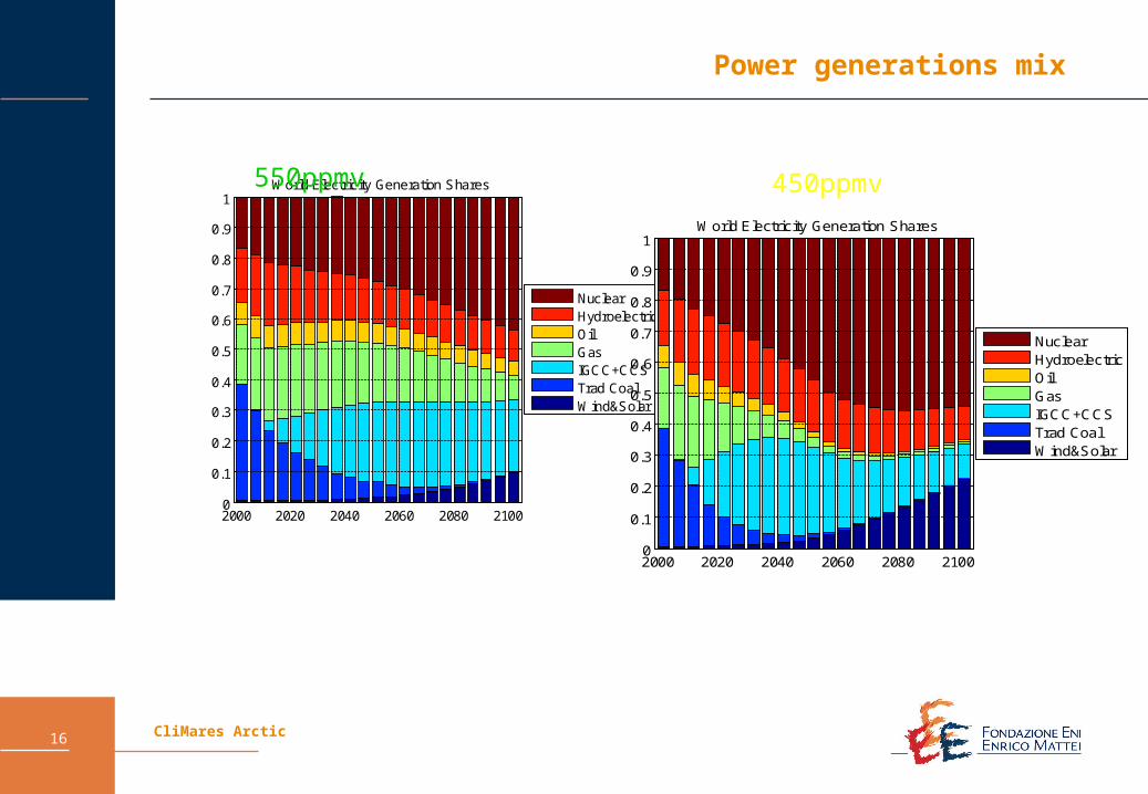
Power generations mix
World Electricity Generation Shares
2000 2020 2040 2060 2080 21000
0.1
0.2
0.3
0.4
0.5
0.6
0.7
0.8
0.9
1
NuclearHydroelectricOilGasIGCC+CCSTrad CoalWind&Solar
World Electricity Generation Shares
2000 2020 2040 2060 2080 21000
0.1
0.2
0.3
0.4
0.5
0.6
0.7
0.8
0.9
1
NuclearHydroelectricOilGasIGCC+CCSTrad CoalWind&Solar
550ppmv 450ppmv

CliMares Arctic17
ICES

CliMares Arctic18
ICES Overview
Recursive dynamic general equilibrium model used for assessment of economic and climate change: Impacts Policies
Top-Down modelInter sectoral factor mobilityInternational tradeInternational investment flowsGHG emissions
CO2 (Carbon dioxide) CH4 (Methane) N2O (Nitrous oxide) SO2 (New - non GHG)
Geographical coverage – up to 87 world regions
CliMares Arctic19
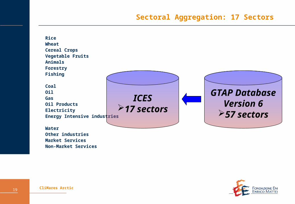
RiceWheatCereal CropsVegetable FruitsAnimalsForestryFishing
CoalOilGasOil ProductsElectricityEnergy Intensive industries
WaterOther industriesMarket ServicesNon-Market Services
Sectoral Aggregation: 17 Sectors
GTAP DatabaseVersion 6
57 sectors
ICES17 sectors

CliMares Arctic20
1° Level
2° Level
3° Level
4° Level
5° Level
6° Level
Supply
OutputOutput
V.A. + Energy
V.A. + Energy Other Inputs
Other Inputs
Domestic
Domestic Foreign
ForeignNatural
Resources
Natural Resource
s LandLand
LabourLabour Capital
+ Energy
Capital +
Energy
CapitalCapital
EnergyEnergy
Non Electric
Non Electric Electric
Electric
CoalCoalNon
Coal
Non Coal
GasGas
OilOil
Petroleum Products
Petroleum Products
Domestic
Domestic Foreign
Foreign
Domestic
Domestic Foreign
Foreign
Domestic
Domestic Foreign
Foreign Domestic
Domestic Foreign
Foreign
DomesticDomestic
ForeignForeign
Reg 1
Reg 1
Reg n
Reg n
Reg ..
Reg ..
Reg 1
Reg 1 Reg
n
Reg n
Reg ..
Reg ..
Reg 1
Reg 1 Reg
n
Reg n
Reg ..
Reg ..
Reg 1
Reg 1 Reg
n
Reg n
Reg ..
Reg ..
Reg 1
Reg 1 Reg
n
Reg n
Reg ..
Reg ..
Region 1Region 1
Region ...
Region ...
Region nRegion n
Representative Firm - cost minimizingLeontief
CES VAE D
CES KE
CES =0.5 D
CES =1
D
CES =1
D
D
D
M
M
M
M
M
M
CliMares Arctic21
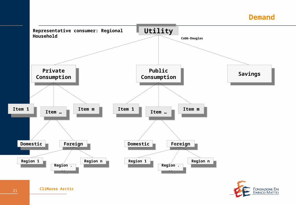
Demand
UtilityUtility
Private Consumptio
n
Private Consumptio
nSavings
Savings
Domestic
Domestic Foreign
Foreign
Region 1Region 1
Region nRegion n
Region ...
Region ...
Item …Item … Item m
Item mItem 1
Item 1
Public Consumptio
n
Public Consumptio
n
Domestic
Domestic Foreign
Foreign
Region 1Region 1
Region nRegion n
Region ...
Region ...
Item …Item … Item m
Item mItem 1
Item 1
Representative consumer: Regional Household
Cobb-Douglas
CliMares Arctic22
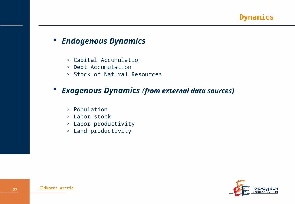
Dynamics
Endogenous Dynamics
> Capital Accumulation> Debt Accumulation> Stock of Natural Resources
Exogenous Dynamics (from external data sources)
> Population> Labor stock> Labor productivity> Land productivity
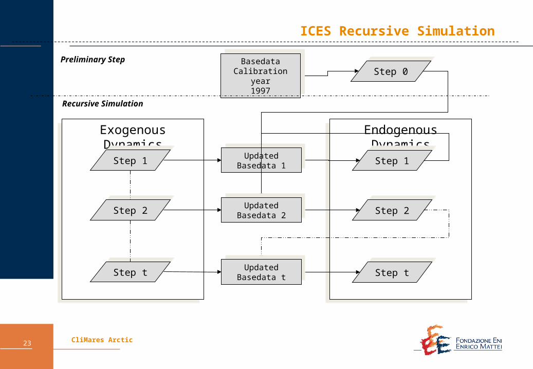
CliMares Arctic23
Endogenous DynamicsEndogenous DynamicsExogenous DynamicsExogenous Dynamics
ICES Recursive Simulation
Preliminary Step BasedataCalibration year
1997
BasedataCalibration year
1997
Step 0Step 0
UpdatedBasedata 1Updated
Basedata 1Step 1Step 1
UpdatedBasedata 2Updated
Basedata 2Step 2Step 2Step 2Step 2
Step 1Step 1
UpdatedBasedata tUpdated
Basedata tStep tStep tStep tStep t
Recursive Simulation
CliMares Arctic24
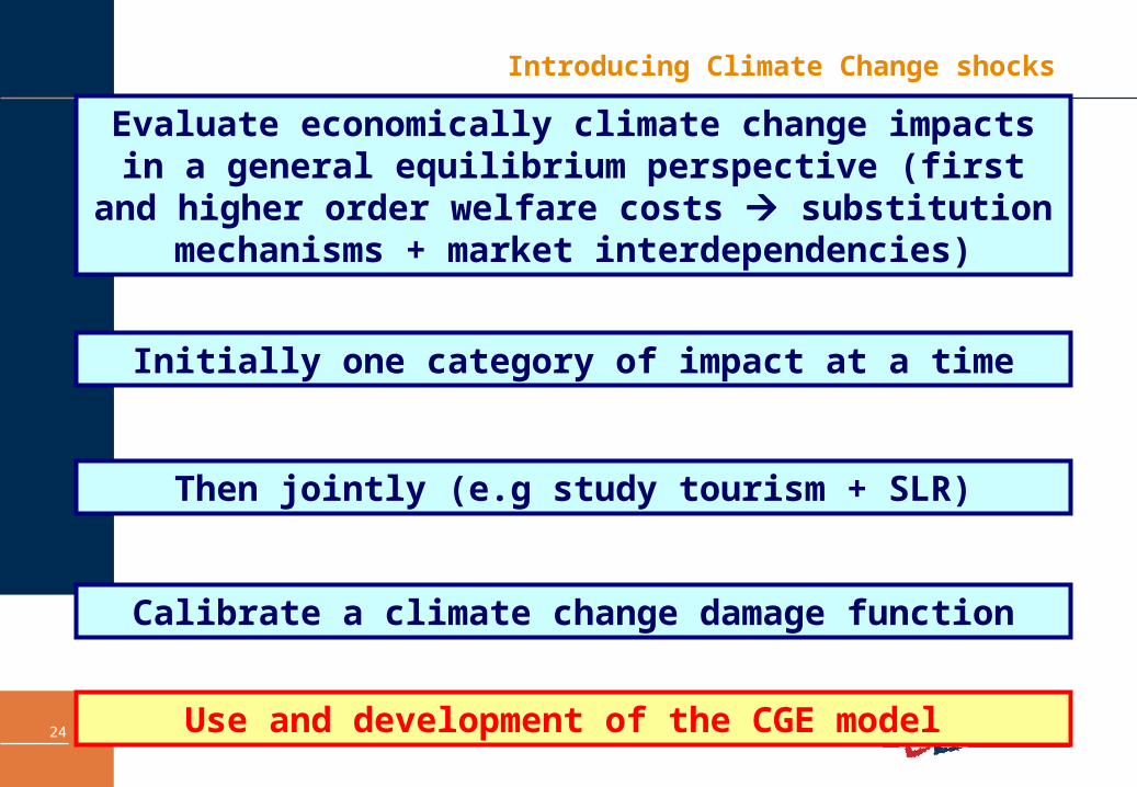
Introducing Climate Change shocks
Evaluate economically climate change impacts in a general equilibrium perspective (first and higher order
welfare costs substitution mechanisms + market interdependencies)
Initially one category of impact at a time
Then jointly (e.g study tourism + SLR)
Use and development of the CGE model
Calibrate a climate change damage function
CliMares Arctic25
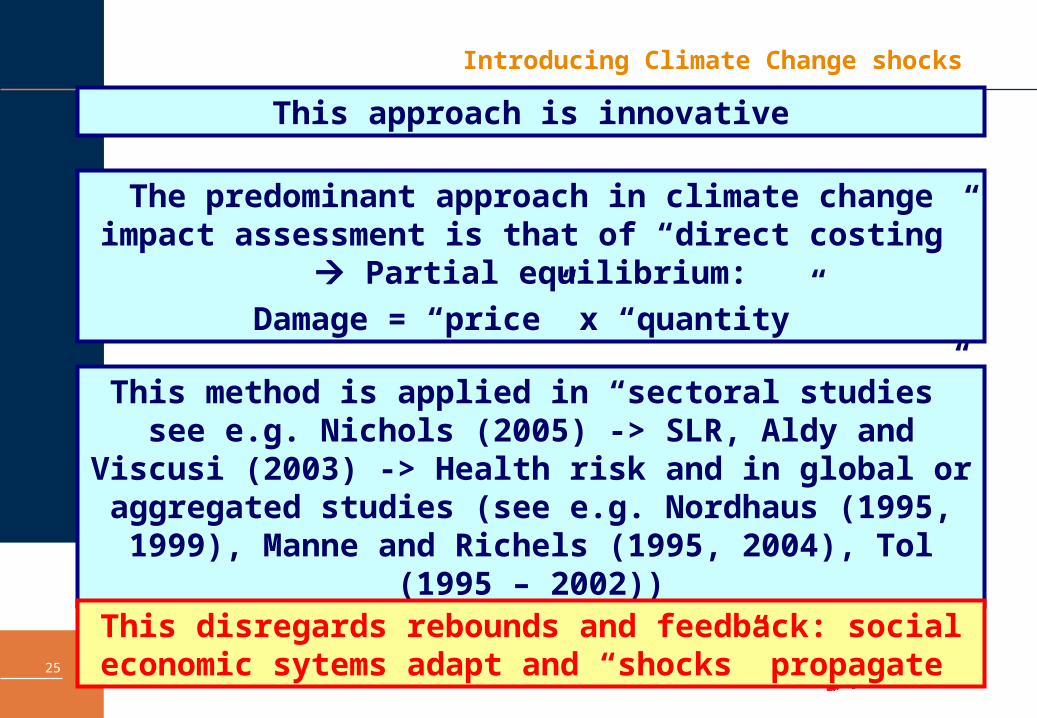
Introducing Climate Change shocks
This approach is innovative
The predominant approach in climate change impact assessment is that of “direct costing” Partial
equilibrium:
Damage = “price” x “quantity”
This method is applied in “sectoral studies” see e.g. Nichols (2005) -> SLR, Aldy and Viscusi (2003) -> Health
risk and in global or aggregated studies (see e.g. Nordhaus (1995, 1999), Manne and Richels (1995, 2004),
Tol (1995 – 2002))
This disregards rebounds and feedback: social economic sytems adapt and “shocks” propagate

CliMares Arctic26
Introducing Climate Change shocks
Integrated Assessment and Modularity
Global Circulation
Models
Climate Change and Variability
Environm.Impact Models
• Temp. increase• Temp. rate of change• Precipitation• Sea level rise
Disentangle Climate Change in (some) Physical Impacts
• Loss of land (sq. Km.)• Changes in tourism flows • Changes in crop yields• .......................
Economic (GE)
Model
Provides welfare evaluation of physical
impacts+
Feedback on the environment
(e.g. emissions)

CliMares Arctic27
Introducing Climate Change shocks
Regional Increase in TemperatureRegional Increase in Temperature
Changes in Households’ demand for “energy” commodities. (Changes in Heating/cooling patterns)
Changes in Households’ demand for “energy” commodities. (Changes in Heating/cooling patterns)
Changes in Households’ preferences for some locations
Changes in Households’ preferences for some locations
Changes in Tourism flowsChanges in Tourism flows
Changes in regional incomeChanges in regional income
OriginOrigin Effect/modelled asEffect/modelled as
Changes in demand for “Market Services” commodity
Changes in demand for “Market Services” commodity

CliMares Arctic28
The difference between direct and general equilibrium cost
-0.012
-0.010
-0.008
-0.006
-0.004
-0.002
0.000
USA CAN WEU JPK ANZ EEU FSU MDE CAM SAM
Land loss value as % of GDP
Final impact on GDP
-0.25
-0.20
-0.15
-0.10
-0.05
0.00
SAS SEA CHI NAF SSA SIS
Land loss value as % of GDP
Final impact on GDP

CliMares Arctic29
Tourism Alone
Imposed Endogeno
us USA -0.874 -1.259 1.457 -0.365 -0.0015 -0.511 -0.626CAN 0.459 0.755 -1.381 0.211 -0.0004 0.420 -0.116WEU 0.883 1.357 -2.287 0.378 0.0556 0.331 0.238JPK 5.639 8.096 -14.760 2.779 -0.1768 3.768 3.810ANZ -1.530 -2.096 3.475 -0.696 0.0493 -0.063 -0.654EEU -3.172 -4.683 3.255 -1.169 -0.1068 -0.803 -0.999FSU -0.024 -0.073 0.052 -0.011 -0.0311 -0.135 -0.390MDE -5.974 -8.600 8.295 -2.074 0.0030 -2.279 -1.960CAM -5.519 -7.980 7.518 -2.387 -0.1139 -1.030 -1.805SAM -1.521 -2.015 1.583 -0.558 -0.0027 -0.100 -1.161SAS -1.532 -1.794 1.102 -0.453 0.0251 0.596 -0.507SEA -5.452 -7.057 6.854 -1.629 -0.0324 -0.825 -0.620CHI -6.777 -8.020 2.731 -1.129 -0.0442 -1.127 -0.854NAF -3.204 -4.179 1.314 -0.646 -0.1614 -0.795 -0.640SSA -3.068 -4.122 2.993 -1.053 -0.0079 -0.359 -0.951SIS -12.251 -18.984 17.001 -5.990 -0.5330 -7.522 -7.852
Market services demand
Other goods/services dem.
Income transfers
GDP Terms of
TradeInvest. Flows
Reference Year 2050: % changes wrt baseline
CliMares Arctic30
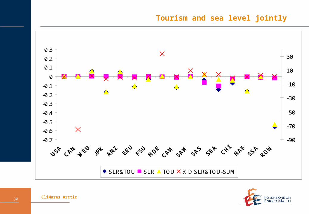
Tourism and sea level jointly
-0.7
-0.6
-0.5
-0.4
-0.3
-0.2
-0.1
0
0.1
0.2
0.3
-90
-70
-50
-30
-10
10
30
SLR&TOU SLR TOU %D SLR&TOU-SUM