Feeder Performance Analysis with Distributed Algorithm

Lingyun Wang

Thesis submitted to the Faculty of the

Virginia Polytechnic Institute and State University

in partial fulfillment of the requirements for the degree of

Master of Science

in

Computer Engineering

Robert P. Broadwater (Co-Chair),

Binoy Ravindran (Co-Chair),

Yue Wang

April 25, 2011

Blacksburg, Virginia

Keywords: Feeder Performance, Distributed Computing, Electric Power Distribution

System, Diakoptics, Locational Marginal Price (LMP)

Copyright© 2011 Lingyun Wang

Feeder Performance Analysis with Distributed Algorithm

Lingyun Wang

ABSTRACT

How to evaluate the performance of an electric power distribution system unambiguously

and quantitatively is not easy. How to accurately measure the efficiency of it for a whole year,

using real time hour-by-hour Locational Marginal Price data, is difficult. How to utilize

distributed computing technology to accomplish these tasks with a timely fashion is challenging.

This thesis addresses the issues mentioned above, by investigating feeder performance

analysis of electric power distribution systems with distributed algorithm.

Feeder performance analysis computes a modeled circuit’s performance over an entire

year, listing key circuit performance parameters such as efficiency, loading, losses, cost impact,

power factor, three phase imbalance, capacity usage and others, providing detailed operating

information for the system, and an overview of the performance of every circuit in the system.

A diakoptics tearing method and Graph Trace Analysis based distributed computing

technology is utilized to speed up the calculation. A general distributed computing architecture

is established and a distributed computing algorithm is described.

iii

To the best of the author’s knowledge, it is the first time that this detailed performance

analysis is researched, developed and tested, using a diakoptics based tearing method and

Graph Trace Analysis to split the system so that it can be analyzed with distributed computing

technology.

iv

To my beloved parents

Guoqing Wang and Daogui She

v

Acknowledgements

I would like to thank my advisor Dr. Robert Broadwater for his support, encouragement,

and assistance both in my research and in writing this thesis. It has always been enjoyable to

work with him and I have been continuously inspired by his erudition, patience and dedication.

I would like to thank Electric Distribution Design (EDD) Inc. for providing facilities to finish

this research work.

I would also want to thank Dr. Binoy Ravindran and Dr. Yue Wang for serving on my

advisory committee.

My appreciation is extended to my fellow graduate students in my group and other

friends I have met so far for their friendship during my study in Virginia Tech.

Specially, I am deepest grateful to my wife, Jiadong Jin and my parents-in-law, Jiansheng

Jin and Yanfei Yao for their endless love and support.

vi

Table of Contents

CHAPTER 1 Introduction .............................................................................................................. 1

1.1 Overview .......................................................................................................................... 1

1.2 Challenges in Feeder Performance Analysis with Distributed Computation ................... 3

1.3 Literature Review ............................................................................................................. 5

1.3.1 Computer-Aided Analysis of Electric Power Distribution Systems ........................... 5

1.3.2 Distributed Computing ............................................................................................. 8

1.4 Thesis Outline ................................................................................................................. 10

CHAPTER 2 Feeder Performance Analysis ................................................................................. 12

2.1 Introduction.................................................................................................................... 12

2.2 Feeder Performance Analysis Implementation ............................................................. 13

2.2.1 Locational Marginal Pricing (LMP) Data Analysis.................................................... 15

2.2.2 Power Flow Analysis ............................................................................................... 19

2.2.3 Performance Analysis ............................................................................................. 20

2.3 Alternative Design Evaluation through Feeder Performance Analysis .......................... 28

vii

2.4 Feeder Performance Analysis Case studies .................................................................... 30

2.5 Challenges of Feeder Performance Analysis .................................................................. 46

CHAPTER 3 Feeder Performance Analysis with Distributed Algorithm ..................................... 48

3.1 Introduction.................................................................................................................... 48

3.1.1 Introduction to distributed systems and distributed computing ........................... 48

3.1.2 Diakoptics, the method of system tearing ............................................................. 50

3.2 Distributed computing architecture in DEW .................................................................. 51

3.2.1 Graph Trace Analysis ............................................................................................... 53

3.2.2 GTA Notation for Distributed Algorithm ................................................................. 57

3.3 Feeder Performance Analysis with Distributed Algorithm Case Studies ....................... 59

CHAPTER 4 Conclusions and Future Work ................................................................................. 63

4.1 Conclusion ...................................................................................................................... 63

4.2 Future Work ................................................................................................................... 64

References……………………………………………………………………………………………………………………………….66

viii

List of Figures

Figure 1.1 Electric Power System .................................................................................................... 1

Figure 2.1 Feeder Performance Analysis Overview ...................................................................... 14

Figure 2.2 LMP Data Analysis ........................................................................................................ 17

Figure 2.3 Feeder Performance Analysis Flow Chart .................................................................... 21

Figure 2.4 Using Feeder Performance to Evaluate Alternative Feasible Designs ......................... 29

Figure 2.5 Example power distribution system ............................................................................ 33

Figure 2.6 Feeder Performance Analysis Interface ....................................................................... 33

Figure 2.7 Sample Circuit Annual Load Plot .................................................................................. 34

Figure 2.8 Sample Circuit Annual Loss Plot ................................................................................... 34

Figure 2.9 Sample Circuit Annual LMP Value Plot ........................................................................ 35

Figure 2.10 Sample Circuit Annual Cost Plot ................................................................................ 35

Figure 2.11 Sample Circuit Annual Efficiency Plot ........................................................................ 36

Figure 2.12 Sample Circuit Annual Phase A Loss Plot ................................................................... 36

Figure 2.13 Sample Circuit Annual Phase A Cost Plot ................................................................... 37

Figure 2.14 Sample Circuit Annual Power Factor (A) Plot ............................................................ 37

Figure 2.15 Sample Circuit Annual Maximum Power Factor Deviation Plot ................................ 38

Figure 2.16 Sample Circuit Annual Phase Imbalance Plot ............................................................ 38

Figure 2.17 Sample Circuit Annual Maximum Imbalance Plot ..................................................... 39

Figure 2.18 Sample Circuit Annual Smallest Single Phase Capacity Plot ...................................... 39

Figure 2.19 Sample Circuit Annual Smallest Three Phase Capacity Plot ...................................... 40

Figure 2.20 Sample Circuit Phase A Current Plot .......................................................................... 40

Figure 2.21 Sample Circuit Smallest Phase A Customer Level Voltage Plot ................................. 41

Figure 2.22 Sample System Annual Efficiency Factor Summary Plot ........................................... 41

Figure 2.23 Sample System Annual Energy Loss Summary Plot ................................................... 42

Figure 2.24 Sample System Annual Loss Cost Summary Plot ....................................................... 42

Figure 2.25 Sample System Annual Energy Supplied Summary Plot ............................................ 43

Figure 2.26 Sample System Annual Phase A Energy Loss Summary Plot ..................................... 43

Figure 2.27 Sample System Annual Phase A Cost Summary Plot ................................................. 44

Figure 2.28 Sample System Annual Average Maximum Imbalance Summary Plot ..................... 44

Figure 2.29 Sample System Annual Average Maximum Power Factor Deviation Summary Plot 45

Figure 3.1 Distributed Systems ..................................................................................................... 49

Figure 3.2 Diakoptics for Distributed Computing ......................................................................... 51

Figure 3.3 Distributed Computing Architecture in DEW ............................................................... 52

Figure 3.4 Sample Circuit for Illustrating GTA [19], [used with permission] ................................ 54

Figure 3.5 Start Componet in DEW ............................................................................................... 55

ix

Figure 3.6 Sample System to Be Separated .................................................................................. 56

Figure 3.7 Dividing the System in DEW Flow Chart ..................................................................... 57

Figure 3.8 Distributed Algorithm Flow Chart ................................................................................ 59

Figure 3.9 Eight machines used for distributed computing .......................................................... 60

Figure 3.10 Distributed Algorithm Performance Plot ................................................................... 61

x

List of Tables

Table 2.1 MISO LMP Data Format ................................................................................................. 16

Table 2.2 Sample Nonstandard LMP Data .................................................................................... 18

Table 2.3 Sample of Standard LMP Data Format .......................................................................... 18

Table 2.4 System Improvement by Phase Balancing (1) ............................................................... 45

Table 2.5 System Improvement by Phase Balancing (2) ............................................................... 46

Table 2.6 System Improvement by Phase Balancing (3) ............................................................... 46

Table 2.7 System Improvement by Phase Balancing (4) ............................................................... 46

Table 3.1 Basic Iterators Used in GTA ........................................................................................... 53

Table 3.2 Iterators for Sample Circuit [19], [used with permission] ............................................ 54

Table 3.3 GTA Operations Used in Distributed Algorithm ............................................................ 58

Table 3.4 Configuration Information for the Eight Feeder Performance ..................................... 60

Table 3.5 Configuration Information for the Circuit Server.......................................................... 60

Table 3.6 Processing Time and Speed-Up for Feeder Performance Analysis with Distributed

Algorithm ...................................................................................................................................... 61

1

CHAPTER 1 Introduction

1.1 Overview

In 1882, the first electric power station, Pearl Street Electric Station in New York City,

went into operation, symbolizing the birth of the electric utility industry [1]. Since then, this

industry has expanded remarkably with generation stations and transmission and distribution

networks spreading across the whole country as energy is expected to be increasingly

converted to electricity [2].

Figure 1.1 illustrates the electric power system and its major systems, including

generation system, transmission system and distribution system.

Figure 1.1 Electric Power System

In past years, the analysis of the high-voltage transmission systems drew the major

attention of researchers and engineers in the electric power industry while little effort was put

2

into the analysis of the distribution system [3], especially the detailed performance analysis of

such systems.

It is reported in [4] that the electric power distribution system can account for up to 60

percent of the total capital budget and 20 percent of the operating cost, and the distribution

system can be 80 percent larger than the transmission system [5]. So, it is critical for the

electric utility industry to understand the overall performance of the electric power distribution

system as the analysis of these systems has been a very important part of the overall planning

of power systems. A viable and optimized plan can not only bring great social benefits by

assuring that the growing demand for electricity of customers is satisfied, but also generate

vast economic benefits by dramatically reducing the cost, with the most conservative estimate

by 5 to 10 percent [4].

In [3], the author points out that distribution planners must accomplish the task of how to

identify the goals for their system by clarifying what exactly constitutes “satisfactory

performance” and how is that measured both unambiguously and quantitatively. What is more,

a reasonable performance analysis can also help planners to target the best design from among

the thousands or even tens of thousands of feasible designs that might work for their system

and fully exploit every opportunity for savings or improvement as it can be a truly daunting task

considering the increasing cost of additions and modifications and the limitation of resources.

Electric power distribution systems are complicated combinatorial entities, consisting of

hundreds of thousands of individual circuit elements. By taking advantage of modern

computational tools which have the ability to accurately model the operating characteristics of

3

unbalanced three-phase distribution feeders, it is possible to conduct the analysis of electric

power distribution system in a more detailed manner.

Various computer programs have been developed to assist engineers in electric power

system analysis, including load estimation, power flow, capacitor design, phase balancing and

reconfiguration analysis, etc. However, detailed performance analysis that takes into account

hourly load variations of electrical power distribution systems has never been conducted. Thus,

feeder performance analysis, which can analyze and evaluate the efficiency of electric power

distribution systems over 8760 hours for non-leap years (8784 hours for leap years), using real

time hour-by-hour Locational Marginal Prices data, is to be investigated here.

As extensive computation on the electric power distribution model is needed in order to

accomplish feeder performance analysis, distributed computation technology could be utilized

to speed up the computation, considering the fact that there exist points in the power

distribution system which can decompose the whole system into several independent

subsystems naturally. With distributed computation technology, multiple autonomous

computers and storage devices as well as databases are organized together to interactively co-

operate with each other to achieve a common goal.

1.2 Challenges in Feeder Performance Analysis with Distributed

Computation

The challenges in feeder performance analysis with distributed computation are

summarized as the following:

4

Modeling

To have a proper model of an electric power distribution system is not an easy task. There

are three aspects in terms of a proper model.

The model reflects the real world, considering all the important attributions of

the system. In electric power distribution systems, this means the system

topology information, component configuration information, system load

information [6], and power flow information.

The model cannot be too complicated by considering every possible attribution

of the system.

The volume of data involved for modeling the electric power distribution system

is huge, and how to prepare the correct data is an intimidating task. Garbage in,

garbage out would be one of most unavoidable problems if the data itself is

incorrect. Actually, as indicated in [7], there is very limited actual data about the

system for modeling and analysis due to the fact that the distribution system is

designed to operate without much monitoring and control. Fortunately, the

smart grid technology arising recently brings hope [8].

This thesis is not dedicated to solving the modeling problem of electric power distribution

systems. However, without a proper model, it is not even possible to conduct the detailed

performance analysis of the electrical power distribution system.

5

Computation Time

Modeling of an electrical power distribution system requires large amounts of computer

memory, and it is typically time consuming to conduct computation on the entire model

Generality

Different utilities usually have different system topology structures, component

configurations and particularly, data information. For example, Locational Marginal Price is a

very important data source in order to evaluate the cost of the operation of electric power

distribution systems. However, the format for the LMP data varies among Independent System

Operators (ISOs) [9] [10]. How to conduct performance analysis on electric power distribution

systems operated by different utilities needs to be addressed.

1.3 Literature Review

A literature search has been performed in the areas listed below:

Computer –Aided analysis of electric power distribution systems

Distributed Computing

1.3.1 Computer-Aided Analysis of Electric Power Distribution Systems

Various innovative computer-aided analysis of electrical power distribution systems have

been researched and implemented. Computer-aided tools can be categorized into three groups

as follows:

6

Modeling tools

Analysis tools

Design tools

Modeling tools provide the computer software framework for electric power distribution

analysis. In papers [11]- [18], an Integrated System Model (ISM) which aims to tie the various

utility data systems, including Geography Information System (GIS), Supervisory Control and

Data Acquisition (SCADA) system, billing system, etc., are discussed. The concept of integrated

modeling considers using results from multiple, fundamental analysis applications. The

fundamental architecture, programming data structures and algorithms are addressed in [19]-

[21], especially Graph Trace Analysis (GTA), a multidiscipline approach that uses generic

algorithms and a common model-based analysis framework.

Basic analysis tools for electric power distribution systems are intended to predict or

evaluate the key attributions of the system such as the load, impedance, voltage, currents, real

and reactive power flows, efficiency, etc. Analysis tools are usually built on top of the modeling

tool. The most fundamental analysis tools include load estimation, impedance analysis, and

power flow analysis. Other analysis tools may include, but are not limited to, fault analysis,

flicker analysis, reliability analysis, phase prediction, harmonic analysis and feeder performance

analysis. In [22], load estimation analysis is conducted by using load research data to calculate

the diversity factors and KWHR-to-peark-KW conversion factors, which aims to predict the time

at which the daily peak KW demand, for a specific class of customer, will occur. It is suggested

in this paper that one of the most efficient ways of estimating the peak load is by dividing the

7

customers into classes based on their usage patterns. Cable impedance analysis is studied in [23]

by comparing approximate impedance calculations used by utilizes in distribution networks

with exact calculations. The ISM power flow analysis as described in [24] presents a sweep-

based, multi-phase power flow method for solving general distribution networks that can be

heavily meshed and include transformers in the loops. Furthermore more, it is demonstrated

that it can solve both IEEE standard transmission and distribution problems, which are solved

with different algorithms traditionally. Fault analysis and reliability analysis based on the

framework proposed in [11]-[18] are described in [25], [26] and [27]. For the phase prediction

analysis, a low cost, algorithmic approach for estimating the phasing of laterals is presented in

[28].

The design tools are oriented to help utilities make decisions about how to build or

upgrade the system. Common design analysis includes reconfiguration, phase balancing,

capacitor design, and protection design, to name a few. Authors in [29] introduce and compare

four algorithms by which the reconfiguration for restoration of an arbitrary number of

interdependent critical infrastructure systems can be achieved. An object-oriented analysis of

distribution system reconfiguration for power restoration is discussed in [30] and a heuristic,

nonlinear constructive method is described in [31]. Phase balancing analysis, which can

recommend how to connect single and double phase laterals to the three phase spine, is

explained in [32]. Literatures related to the design issues of how to optimally locate and size

capacitor banks is found in [33]-[35].

8

1.3.2 Distributed Computing

The literature review about the topic of distributed computing is organized as follows:

Traditional theoretical foundations of distributed computing

Distributed computing in analysis of electric power systems

Diakoptics: the method of tearing

In terms of theoretical foundations of distributed computing, people usually talk about

distributed algorithms [36]. A distributed algorithm is an algorithm designed to run on

distributed systems. Since 1960s, researchers have conducted research on different topics

concerning distributed computing algorithms.

Mutual exclusion

Paper [37] presented the first solution to the mutual exclusion problem, which is

considered as the start of the field of concurrent and distributed algorithms [38]. M. Crummey

and M.L.Scotty proposed a practical mutual exclusion algorithm in [39], which generates O(1)

remote references per lock acquisition, independent of the number of processors attempting to

acquire the lock. This algorithm is recognized as one of the most influential and practical mutual

exclusion algorithms [40].

Consensus

In [41] and [42] the authors introduced and studied the Byzantine fault tolerance model,

pointing out that agreement between computers cannot be made if at least 1/3 of the nodes

are faulty. It is shown in [43] that it is impossible to achieve distributed consensus when one

9

faulty node exists in an asynchronous system. Paper [44] introduced the concept of partial

synchrony in a distributed system and further studied the consensus problem in the partial

synchronous system.

Distributed computing technology has also been applied in the analysis of electric power

distribution systems, especially for the power flow calculation, which usually requires extensive

computation. In [45], distributed algorithms for both radial and looped load flows for

unbalanced, muti-phase electric power distribution systems are proposed, implemented and

tested. An optimized contingency analysis program running in a distributed computation

environment is presented in [46].

The Diakoptics method was presented by Gabriel Kron in the book entitled ‘Diakoptics:

The Piecewise Solution of Large-Scale Systems’ in 1963 *47+. The terminology diakoptics

originated from the Greek words “kopto” which means to tear and “dia” which means systems.

Hence diakoptics can be interpreted as system-tearing .

The main idea of diakoptics is to decompose physical systems, typically electrical circuits,

into subsystems with the particular property that the subsystems overlap on their boundaries.

Each subsystem can be analyzed and solved separately as if the other subsystems were non-

existent. Then the solution to each subsystem is recombined to give an exact overall solution

[48].

The original purpose of diakoptics was not to distribute computing, but to facilitate the

solution of complex problems that cannot be solved in one piece .When there were no digital

10

computers with the capability to handle the calculation of large and complicated electrical

circuits in one piece, Diakoptics was an effective way to approach the overwhelmingly difficult

task. However, with the development of computer technology, especially computer network

technology, Diakoptics, the method of tearing provides a natural way to make good use of

distributed computing for systems with natural points of separation [49]. In particular, this

technique divides the computation into relatively independent local parts, which may be done

without any interprocessor communication, and thus the mutual exclusion and consensus

problems are solved naturally at the same time.

1.4 Thesis Outline

The remainder of this thesis consists of three chapters.

Chapter two explains in detail the feeder performance analysis of electric power

distribution systems, which computes a circuit's performance parameters over an entire year,

listing key circuit performance parameters for all hours of the year. Power flow, the foundation

of feeder performance analysis, is introduced briefly. Locational Marginal Prices analysis is also

explained. A case study of a real word electric power distribution system is presented.

Chapter three discusses feeder performance analysis with distributed computation. The

disturbed computation architecture is illustrated and a Graph Trace Analysis based description

of the operation of the distributed computing algorithm is presented. A case study of a real

world electric power distribution system is then conducted.

11

Chapter four presents conclusions and outlines possible further research.

12

CHAPTER 2 Feeder Performance Analysis

2.1 Introduction

Electric power distribution systems comprise the parts of an electrical power system

between the subtransmission system and the consumers’ service. The goal is to transport the

power from the transmission system to the customer efficiently, effectively, economically, as

well as reliability.

By taking advantage of modern computing technology, it is possible to establish a

detailed model for the electric power distribution system. Based on the model, feeder

performance analysis of an electric power distribution system calculates feeder energy losses

and their cost, three phase imbalance, as well as capacity usage, etc. It can measure the

efficiency of feeders over 8760 hours for non-loop years (8784 hours for leap years), using real

time hour-by-hour Locational Marginal Pricing (LMP).

Incorporated with phase balancing analysis and other design tools, it can evaluate system

improvement projects with concrete cost data. It is also possible to use feeder performance

analysis to select the most economical designs.

This chapter first introduces the Distributed Engineering Workstation, the platform in

which feeder performance analysis is developed, and the overall architecture of feeder

performance analysis. Then, Locational Marginal Pricing (LMP) analysis is discussed, followed by

a brief introduction of power flow analysis. After that, the feeder performance analysis is

explained in detail and using feeder performance to evaluate alternative feasible designs is

13

illustrated. A case study of feeder performance analysis using a real world electrical power

distribution system is conducted. Finally, the challenges of feeder performance analysis are

summarized.

2.2 Feeder Performance Analysis Implementation

Feeder Performance analysis is built inside the Distributed Engineering Workstation

(DEW). DEW is a multidiscipline, open-architecture environment, providing researchers the

ability to conduct distribution systems engineering studies. The open architecture framework

of DEW supports future expansion, which allows for applications to utilize the results from

other applications [12]. An Application Programmer Interface (API) [17] is supplied for

integrating application modules into the framework without affecting the operation of the

other parts of DEW via the use of dynamic link libraries (DLLs).

The Feeder Performance DEW analysis is built upon Power Flow analysis by requesting

results from the power flow. Figure 2.1 provides an overview of the software architecture of

the Feeder Performance application.

In Figure 2.1, Locational Marginal Pricing data is obtained from the internet first. This

data is then converted to the standard DEW Locational Marginal Price data format through an

LMP data analysis program. Using hourly Locational Marginal Price information, the Feeder

Performance analysis can measure the efficiency of feeders over 8760 hours per year.

14

Figure 2.1 Feeder Performance Analysis Overview

For the performance evaluation of the electric power distribution system, the equipment

load, power supply, power factor, losses, voltage values, costs and others are of interest to

distribution engineers. Although the power flow analysis can supply the basic information of

these attributes, the power flow analysis results are not enough to obtain a complete view of

the performance of the whole system. By incorporating the power flow analysis together with

the Locational Marginal Price data, feeder performance analysis of the power distribution

system calculates feeder energy losses and their associated loss cost along with summary

results concerning three-phase imbalance and equipment capacities. Engineers using feeder

performance analysis with actual energy cost data generated by power flow analysis can

15

evaluate system improvement projects with concrete cost benefits that derive from the time

varying load pattern and costs and not just peak load values.

2.2.1 Locational Marginal Pricing (LMP) Data Analysis

LMP, the abbreviation of Locational Marginal Price, is the theoretical price of electricity at

each node on the network, in other words, the price of energy at a location. As described in

[50], a more formal definition of LMP is: “the marginal cost of supplying, at least cost, the next

increment of electric demand at a specific location (node) on the electric power network, taking

into account both supply (generation/import) bids and demand (load/export) offers and the

physical aspects of the transmission system including transmission and other operational

constraints.”

It has the following characteristics [51]:

LMP is the cost of supplying an increment of load at a particular location.

LMPs are usually produced as a result of economic dispatch, which is the “operation of

generation facilities to produce energy at the lowest cost to reliabily serve consumers,

recognizing any operational limits of generation and transmission facilities” *52+.

Bid-based : In general, by matching offers from generators to bids from consumers at

each node, a supply and demand equilibrium price is established, and the LMP in the

day-ahead market is determined [53]

Security constrained: the LMP calculation is subject to the constraints that exist on the

transmission network, which may be caused when a potential overload occur due to a

contingent event

16

The LMP data is accessible from websites maintained by the Independent System

Operators (ISO). The format for the LMP data varies by different ISOs. For example, the format

of LMP data supplied by New York ISO (NYISO) [9] is different from the one released by the

Midwest ISO (MISO) [10]. The NYISO records LMP data at intervals varying from one to ten

minutes, while the LMP data provided by MISO is on a constant hourly interval.

It is observed that the LMP data format maintained by MISO is relatively clear, well

organized and easy to understand. Thus, it is suitable to be the prototype of a standard LMP

data format.

The MISO LMP data format is shown in Table 2.1

Table 2.1 MISO LMP Data Format

MARKET_DAY NODE TYPE VALUE HE1 HE2 … HE23 HE24

MARKET_DAY : the date

NODE: the location

TYPE: the type of the node

VALUE: HE1 – HE24 represent the LMP value

HE(X): the LMP value between hour (X-1) and hour X for the given date

For nonstandard LMP data (such as the NYISO data), formula 2.1 is utilized to convert it to

the standard format with the price specified at hourly intervals.

17

∑

(2.1)

where is the LMP value for node , denotes the number of LMP records in the

hour under consideration for node , represents the LMP value for node between

time point and .

The LMP Data Analysis Program flow chart is shown in Figure 2.2.

Figure 2.2 LMP Data Analysis

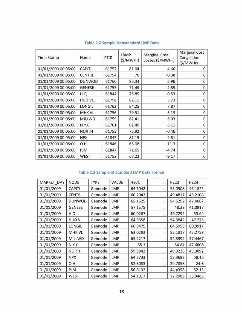
Table 2.2 shows a sample of the nonstandard LMP data and Table 2.3 shows a sample of

the selected standard format for the LMP data.

18

Table 2.2 Sample Nonstandard LMP Data

Time Stamp Name PTID LBMP ($/MWHr)

Marginal Cost Losses ($/MWHr)

Marginal Cost Congestion ($/MWHr)

01/01/2009 00:05:00 CAPITL 61757 81.04 4.66 0

01/01/2009 00:05:00 CENTRL 61754 76 -0.38 0

01/01/2009 00:05:00 DUNWOD 61760 82.34 5.96 0

01/01/2009 00:05:00 GENESE 61753 71.49 -4.89 0

01/01/2009 00:05:00 H Q 61844 75.85 -0.53 0

01/01/2009 00:05:00 HUD VL 61758 82.11 5.73 0

01/01/2009 00:05:00 LONGIL 61762 84.25 7.87 0

01/01/2009 00:05:00 MHK VL 61756 79.51 3.13 0

01/01/2009 00:05:00 MILLWD 61759 82.41 6.03 0

01/01/2009 00:05:00 N.Y.C. 61761 82.49 6.11 0

01/01/2009 00:05:00 NORTH 61755 75.92 -0.46 0

01/01/2009 00:05:00 NPX 61845 81.19 4.81 0

01/01/2009 00:05:00 O H 61846 65.08 -11.3 0

01/01/2009 00:05:00 PJM 61847 71.65 -4.74 0

01/01/2009 00:05:00 WEST 61752 67.22 -9.17 0

Table 2.3 Sample of Standard LMP Data Format

MARKET_DAY NODE TYPE VALUE HE01 … HE23 HE24

01/01/2009 CAPITL Gennode LMP 64.1042 … 53.0508 46.1825

01/01/2009 CENTRL Gennode LMP 60.2042 … 49.4817 43.2108

01/01/2009 DUNWOD Gennode LMP 65.1625 … 54.5292 47.4067

01/01/2009 GENESE Gennode LMP 57.1575 … 48.28 41.0917

01/01/2009 H Q Gennode LMP 60.0267 … 49.7292 53.64

01/01/2009 HUD VL Gennode LMP 64.9658 … 54.3842 47.275

01/01/2009 LONGIL Gennode LMP 66.9475 … 64.5958 60.9917

01/01/2009 MHK VL Gennode LMP 63.0283 … 52.1817 45.2758

01/01/2009 MILLWD Gennode LMP 65.2217 … 54.5992 47.4467

01/01/2009 N.Y.C. Gennode LMP 65.3 … 54.84 47.6608

01/01/2009 NORTH Gennode LMP 59.9842 … 49.9225 43.3092

01/01/2009 NPX Gennode LMP 64.2733 … 53.3692 58.16

01/01/2009 O H Gennode LMP 52.6083 … 29.7858 24.6

01/01/2009 PJM Gennode LMP 56.6192 … 44.4358 52.13

01/01/2009 WEST Gennode LMP 54.1017 … 32.2983 33.9483

19

2.2.2 Power Flow Analysis

Power flow analysis (also called load flow analysis) is applied to a power system model to

compute the voltage magnitude and angle at each bus under steady-state conditions. Real and

reactive power flows for all the equipment interconnecting the buses, as well as equipment

losses, are computed [1].

As the characteristics of transmission networks, which are typically three-phase and

mostly operate balanced, are different from the characteristics of distribution networks, which

can have any number of phases and are usually radial and unbalanced, the power flow of

transmission networks is usually distinct from that of distribution networks.

The power flow algorithm described in [24], solves both IEEE standard transmission and

distribution systems. Building on the analysis results of the power flow, the feeder performance

analysis is developed.

The power flow analysis results which are used in feeder performance analysis are as

follows:

Voltage magnitude at the end of component, in kV

Voltage phase angle, in degrees

Current magnitude at the start of component, in A

Current phase angle, in degrees

Power flow through a component, in kW

Reactive power flow through a component, in kVar

Power Factor associated with complex power flow through a component, in percent

20

Phase imbalance calculated in terms of power flow imbalance

Customer level voltage, in volts

Calculated load for line/cable section, in kW

Percentage of Available Capacity, in percent

2.2.3 Performance Analysis

The Feeder Performance application computes a modeled circuit's performance

parameters over an entire year, listing key circuit performance parameters for all hours of the

year. To the best of our knowledge, it is the first time that this detailed performance analysis is

investigated.

Figure 2.3 illustrates the flow chart of feeder performance analysis.

21

Figure 2.3 Feeder Performance Analysis Flow Chart

The performance analysis results include an hourly based report for every circuit and a

summary report for all circuits in the system.

The hourly based feeder performance analysis results are:

The time for the analysis results

22

The total circuit loading, in kWh

The total circuit losses, in kWh

The applicable LMP for the associated circuit and time point, in dollars/mWh

The cost impact of circuit losses, in dollars

The efficiency for the circuit, in percent

Circuit losses of phase A, in kWh

Circuit losses of phase B, in kWh

Circuit losses of phase C, in kWh

The cost impact of circuit losses of phase A, in dollars

The cost impact of circuit losses of phase B, in dollars

The cost impact of circuit losses of phase C, in dollars

Power factor of phase A, in percent

Power factor of phase B, in percent

Power factor of phase C, in percent

Maximum power factor deviation, which represents the worst performing phase's

power factor deviation from unity, in percent

Phase imbalance calculated in terms of power flow imbalance, in percent

Phase A current at start of circuit, in Amps

Phase B current at start of circuit, in Amps

Phase C current at start of circuit, in Amps

Maximum phase imbalance, which represents the maximum imbalance for the three-

phase portion of circuit only, in Amps

23

Smallest single phase capacity, which represents the minimum available capacity over

all single (and two) phase primary lines and cables, in percent

Unique Identifier (UID) of the component with the smallest single phase capacity, which

can be used to locate the component in the model

Smallest three phase capacity, which represents the minimum capacity over all three

phase primary lines and cables, in percent

UID of the component having the smallest three phase capacity, which can be used to

locate the component in the model

Smallest customer level voltage of phase A, in volts

UID of the component with the smallest customer level voltage of phase A, providing

the location of that component.

Smallest customer level voltage of phase B, in volts

UID of the component with smallest customer level voltage of phase B, which can be

used to locate the component in the model

Smallest customer level voltage of phase C, in volts

UID of the component with smallest customer level voltage of phase C, which can be

used to locate the component in the model.

The loading for circuit at time is represented by and is calculated by formula 2.2

∑ (2.2)

,where is the phase power flow and is the phase circuit losses for circuit

at time point , .

24

The total losses for circuit at time is represented by and is calculated by

formula 2.3.

∑ (2.3)

The cost impact of losses occurred in circuit for the associated time point , ,is

given by formula 2.4.

(2.4)

, where is the LMP price for circuit as calculated in formula 2.1. Circuit needs to be

in the area of node .

The efficiency of the circuit at time point , ,is given by formula 2.5.

(2.5)

The maximum Power Factor deviation of circuit at time point , ,which gives the

worst performing phase's power factor deviation from unity, is determined by formula 2.6.

(2.6)

,where is the phase power factor of circuit at time point , .

The Maximum Phase Imbalance of circuit at time point , , showing the maximum

current imbalance, is calculated from formula 2.7.

(2.7)

25

, where and is the phase, current for circuit at time point ,

and .

The smallest single phase capacity of circuit at time point , , which

demonstrates the minimum available capacity from all single (and two) phase primary lines and

cables is evaluated by formula 2.8.

(2.8)

, where is the available capacity for the single phase (or two phase) component

in circuit at time point and

,

The smallest three phase capacity of circuit at time point , , which demonstrates

the minimum available capacity from all three phase primary lines and cables in the circuit is

evaluated by formula 2.9.

(2.9)

,where is the available capacity for the three component in circuit at time

point ,

26

The smallest customer level phase voltage of circuit at time point , , is

represented by formula 2.10.

(2.10)

, where is the customer level phase voltage for the component in circuit at

time point ,

, all components with customer level voltage

The summary report results for all the circuits provide the following information for each

circuit:

Feeder name

Annual energy loss, in kWh

Annual loss cost, in dollars

Annual energy supplied, in kWh

Annual efficiency factor, in percent

Annual phase A energy loss, in kWh

Annual phase B energy loss, in kWh

Annual phase C energy loss, in kWh

Annual phase A cost, in dollars

Annual phase B cost, in dollars

Annual phase C cost, in dollars

Average max phase imbalance of the circuit for the start of the circuit, in amps

27

Average max power factor deviation of the circuit for the start of the circuit, in percent

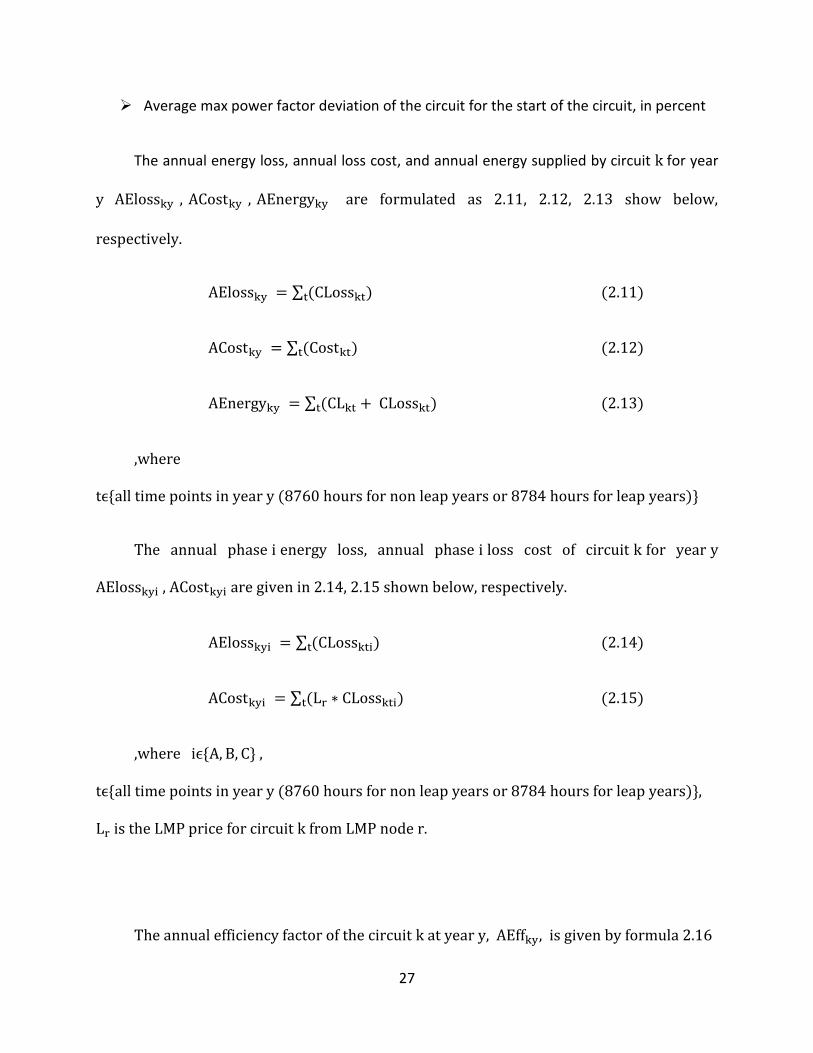
The annual energy loss, annual loss cost, and annual energy supplied by circuit for year

, , are formulated as 2.11, 2.12, 2.13 show below,

respectively.

∑ (2.11)

∑ (2.12)

∑ (2.13)

,where

The annual phase energy loss, annual phase loss cost of circuit for year

, are given in 2.14, 2.15 shown below, respectively.

∑ (2.14)

∑ (2.15)

,where ,

,

is the LMP price for circuit from LMP node .

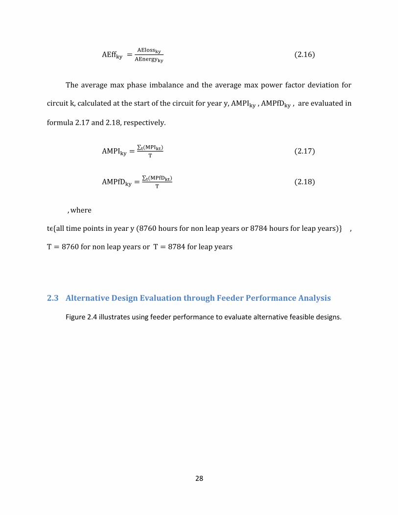
The annual efficiency factor of the circuit at year , , is given by formula 2.16

28

(2.16)

The average max phase imbalance and the average max power factor deviation for

circuit , calculated at the start of the circuit for year , , , are evaluated in

formula 2.17 and 2.18, respectively.

∑

(2.17)

∑

(2.18)

, where

,

2.3 Alternative Design Evaluation through Feeder Performance Analysis

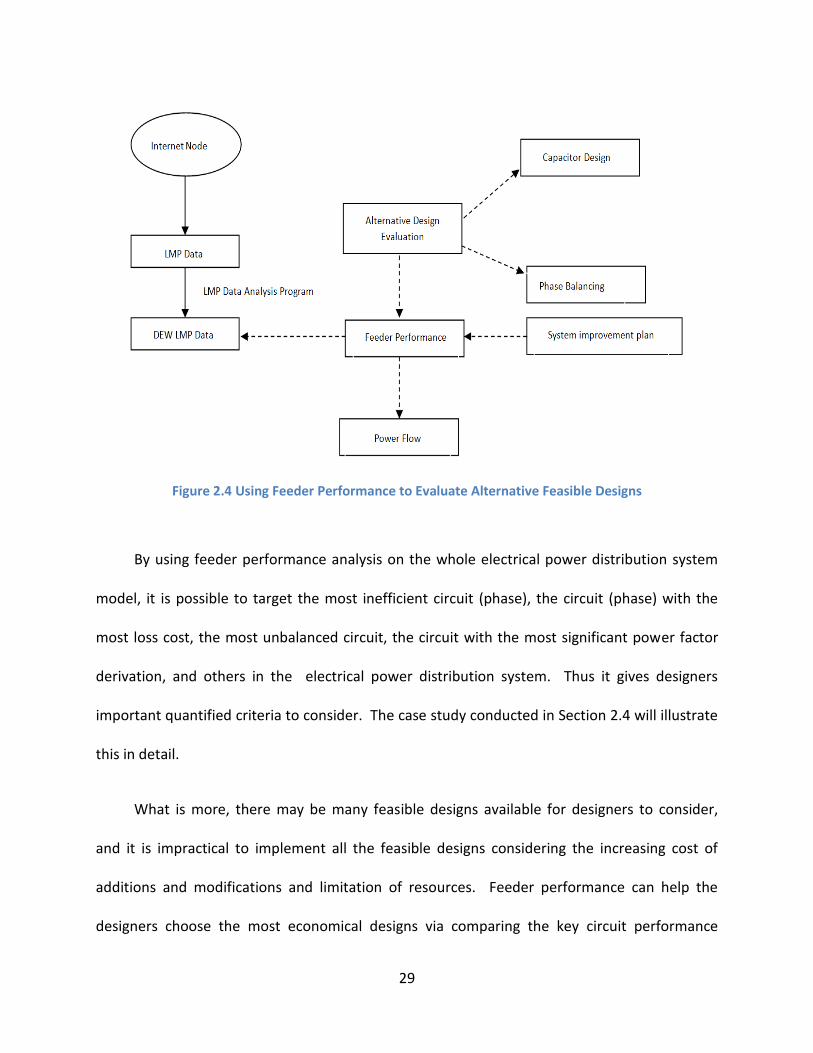
Figure 2.4 illustrates using feeder performance to evaluate alternative feasible designs.

29

Figure 2.4 Using Feeder Performance to Evaluate Alternative Feasible Designs

By using feeder performance analysis on the whole electrical power distribution system

model, it is possible to target the most inefficient circuit (phase), the circuit (phase) with the

most loss cost, the most unbalanced circuit, the circuit with the most significant power factor

derivation, and others in the electrical power distribution system. Thus it gives designers

important quantified criteria to consider. The case study conducted in Section 2.4 will illustrate

this in detail.

What is more, there may be many feasible designs available for designers to consider,

and it is impractical to implement all the feasible designs considering the increasing cost of

additions and modifications and limitation of resources. Feeder performance can help the

designers choose the most economical designs via comparing the key circuit performance

30

parameters. For example, if a circuit needing improvement has significant phase unbalancing

issue while the power factor remains in an acceptable range, it is wise to do phase balancing

instead of capacitor design. Regarding how to choose the most suitable design, the case study

conducted as follows will provide further demonstration.

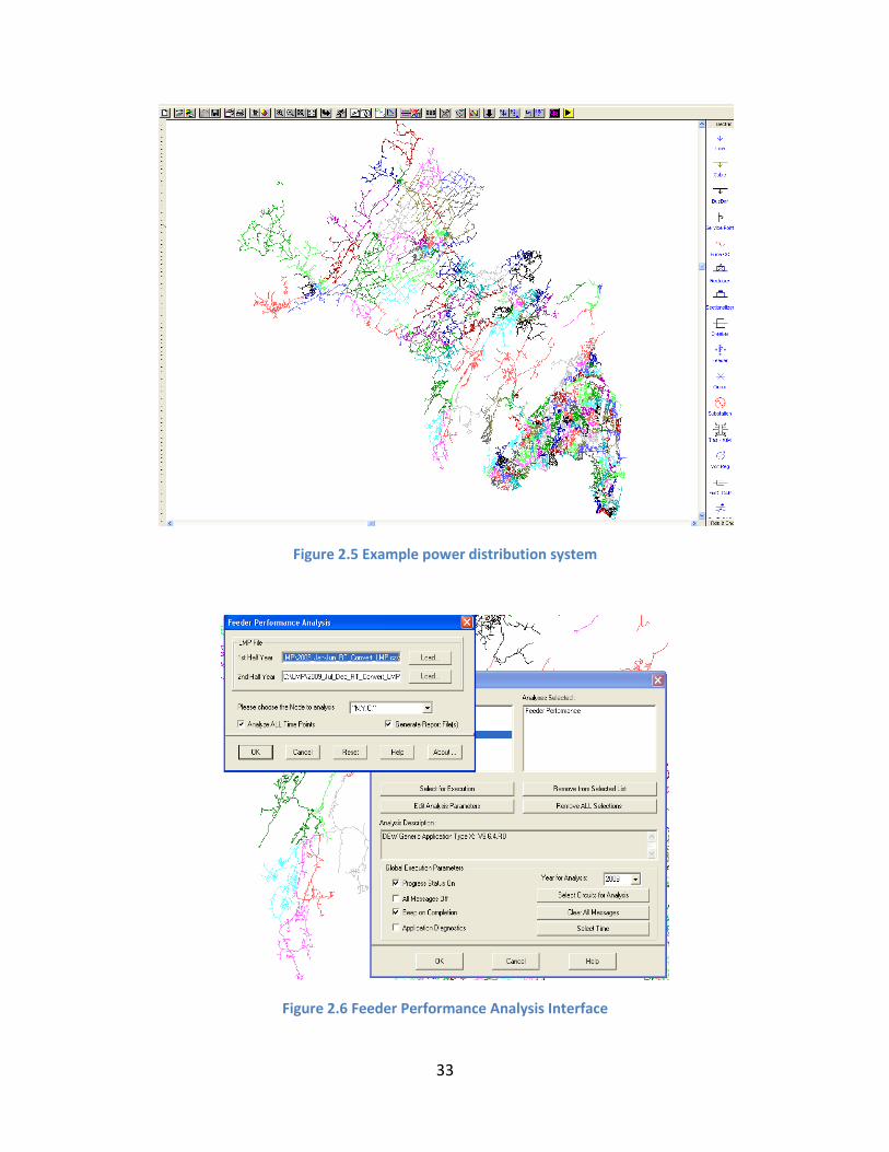
2.4 Feeder Performance Analysis Case studies

Figure 2.5 shows a real-world electrical power distribution system model built in DEW and

Figure 2.6 shows the Feeder Performance Analysis Interface in DEW. The LMP data in Figure 2.6

is downloaded from ISO websites and the location (node) information is indicated by the user.

Feeder Performance Analysis is then utilized on the system shown in Figure 2.5.

Figure 2.7 to Figure 2.21 illustrate the hourly based feeder performance analysis for a

sample circuit in the electrical power distribution system as shown in Figure 2.5.

It is demonstrated in Figure 2.7 that the load demand reaches the peak value in summer

at 5500 kWh to 6200 kWh, causing the maximum loss of the whole year at the same period as

shown in Figure 2.8 at around 160kWh to 210kWh. It also can be concluded that the load

demand is always 20 to 40 percent higher, depending on the season, during the weekends than

during the weekdays of the same month from Figure 2.7.

The annual LMP value as shown in Figure 2.9 is very uneven. It may rise sharply from tens

of dollars/mWh to around 700 dollars/mWh in July and it is also possible to fall dramatically

31

from 100 dollars/mWh to -300 dollars/mWh at the end of June, which means serving an

additional MW of load at that time will reduce the operating cost.

By multiplying the loss of the sample circuit and LMP value of it, the sample circuit annual

cost is plotted in Figure 2.10. By comparing Figures 2.9 and 2.10, it is concluded that the cost is

largely dependent on the LMP value itself.

The annual efficiency of the circuit as plotted in Figure 2.11 remains relatively constantly

at around 97% to 98%, meaning that the operation of the sample circuit is pretty efficient.

It is not so surprising to find in Figure 2.14 that the power factor of phase A of the sample

circuit in summer is lower than that in other seasons in the year by 2 to 8 percent and in Figure

2.15 that the maximum power factor deviation in summer is greater than that in other seasons

in the year by 5 to 9 percent.

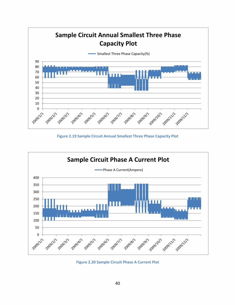
Figure 2.18 makes it clear that the smallest single phase capacity in September is negative,

around -8 percent, implying that some of the single phase laterals in the sample circuit are

overloaded during that time and may need special attention. In Figure 2.20, the phase A

current goes as high as 350A in the summer and the smallest phase A customer level voltage is

drop down to around 105V in the summer as shown in Figure 2.21, verifying the fact that the

summer demand load is large.

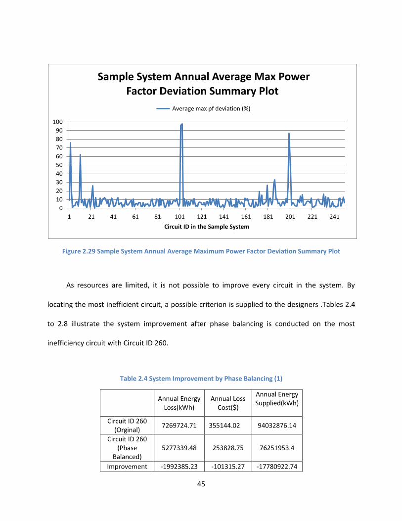
Figures 2.22 to 2.29 show the summary report results for the sample system shown in

Figure 2.5. These plots provide circuit ID in the sample system to the various key performance

32

parameters such as circuit annual efficiency, annual energy loss, annual loss cost, annual

average maximum phase imbalance, and annual average maximum power factor deviation.

There are wild fluctuations in the annual efficiency factor as shown in Figure 2.22, with

the lowest efficiency at ID 250. By comparing Figure 2.22 with Figures 2.23 and 2.24, it is

concluded that the higher the annual efficiency of the circuit, the lower its annual energy loss

and cost are.

Similarly, the system annual maximum phase imbalance as shown in Figure 2.28 and

the system annual maximum power factor deviation as shown in Figure 2.29 are erratic, but the

circuit with the worst performance, in terms of either worst phase balance or power factor

deviation, can be easily located.

33

Figure 2.5 Example power distribution system

Figure 2.6 Feeder Performance Analysis Interface

34

Figure 2.7 Sample Circuit Annual Load Plot

Figure 2.8 Sample Circuit Annual Loss Plot

0

1000

2000

3000

4000

5000

6000

7000

Sample Circuit Annual Load Plot

Circuit Load(kWh)

0

50

100

150

200

250

Sample Circuit Annual Loss Plot

Circuit Loss(kWh)

35

Figure 2.9 Sample Circuit Annual LMP Value Plot

Figure 2.10 Sample Circuit Annual Cost Plot

-400

-200

0

200

400

600

800

Sample Circuit Annual LMP Value Plot

LMP Value (Dollars/mWh)

-60

-40

-20

0

20

40

60

80

100

120

140

Sample Circuit Annual Cost Plot

Cost(Dollars)

36

Figure 2.11 Sample Circuit Annual Efficiency Plot

Figure 2.12 Sample Circuit Annual Phase A Loss Plot

0.968

0.97

0.972

0.974

0.976

0.978

0.98

0.982

Sample Circuit Annual Efficiency Plot

Efficiency of the Circuit

0

20

40

60

80

100

120

Sample Circuit Annual Phase A Loss Plot

Phase A Loss(kWh)

37

Figure 2.13 Sample Circuit Annual Phase A Cost Plot

Figure 2.14 Sample Circuit Annual Power Factor (A) Plot

-30

-20

-10

0

10

20

30

40

50

60

Sample Circuit Annual Phase A Cost Plot

Phase A Cost($)

78

80

82

84

86

88

90

92

94

Sample Circuit Annual Power Factor (A) Plot

Power Factor(A %)

38

Figure 2.15 Sample Circuit Annual Maximum Power Factor Deviation Plot

Figure 2.16 Sample Circuit Annual Phase Imbalance Plot

0

2

4

6

8

10

12

14

16

18

Sample Circuit Annual Max Power Factor Deviation Plot

Max pf deviation (%)

0

0.05

0.1

0.15

0.2

0.25

0.3

Sample Circuit Annual Phase Imbalance Plot

PhImbal

39

Figure 2.17 Sample Circuit Annual Maximum Imbalance Plot

Figure 2.18 Sample Circuit Annual Smallest Single Phase Capacity Plot

0

20

40

60

80

100

120

140

160

Sample Circuit Annual Max Imbalance Plot

Max Imbalance(A)

-20

-10

0

10

20

30

40

50

60

70

80

90

Sample Circuit Annual Smallest Single Phase Capacity Plot

Smallest Single Phase Capacity(%)

40

Figure 2.19 Sample Circuit Annual Smallest Three Phase Capacity Plot

Figure 2.20 Sample Circuit Phase A Current Plot

0

10

20

30

40

50

60

70

80

90

Sample Circuit Annual Smallest Three Phase Capacity Plot

Smallest Three Phase Capacity(%)

0

50

100

150

200

250

300

350

400

Sample Circuit Phase A Current Plot

Phase A Current(Ampere)

41

Figure 2.21 Sample Circuit Smallest Phase A Customer Level Voltage Plot

Figure 2.22 Sample System Annual Efficiency Factor Summary Plot

95

100

105

110

115

120

125

Sample Circuit Smallest Phase A Customer Level Voltage Plot

Smallest Phase A CustV (Volts)

0.78

0.8

0.82

0.84

0.86

0.88

0.9

0.92

0.94

0.96

0.98

1

1 21 41 61 81 101 121 141 161 181 201 221 241

Circuit ID in the Sample System

Sample System Annual Efficiency Factor Summary Plot

Efficiency Factor

42

Figure 2.23 Sample System Annual Energy Loss Summary Plot

Figure 2.24 Sample System Annual Loss Cost Summary Plot

0

1000000

2000000

3000000

4000000

5000000

6000000

7000000

1 21 41 61 81 101 121 141 161 181 201 221 241

Circuit ID in the Sample System

Sample System Annual Energy Loss Summary Plot

Annual Energy Loss(kWh)

0

50000

100000

150000

200000

250000

300000

350000

400000

1 21 41 61 81 101 121 141 161 181 201 221 241Circuit ID in the Sample System

Sample System Annual Loss Cost Summary Plot

Annual Loss Cost($)

43

Figure 2.25 Sample System Annual Energy Supplied Summary Plot

Figure 2.26 Sample System Annual Phase A Energy Loss Summary Plot

0

20000000

40000000

60000000

80000000

100000000

120000000

1 21 41 61 81 101 121 141 161 181 201 221 241

Circuit ID in the Sample System

Sample System Annual Energy Supplied Summary Plot

Annual Energy Supplied(kWh)

0

500000

1000000

1500000

2000000

2500000

3000000

3500000

4000000

4500000

1 21 41 61 81 101 121 141 161 181 201 221 241

Circuit ID in the Sample System

Sample System Annual Phase A Energy Loss Summary Plot

Annual Phase A Energy Loss(kWh)

44

Figure 2.27 Sample System Annual Phase A Cost Summary Plot

Figure 2.28 Sample System Annual Average Maximum Imbalance Summary Plot

0

50000

100000

150000

200000

250000

300000

350000

1 21 41 61 81 101 121 141 161 181 201 221 241

Circuit ID in the Sample System

Sample System Annual Phase A Cost Summary Plot

Annual Phase A Cost($)

0

50

100

150

200

250

300

350

400

450

500

1 21 41 61 81 101 121 141 161 181 201 221 241

Circuit ID in the Sample Circuit

Sample System Annual Average Max Imbalance Summary Plot

Average max imbalance (A)

45

Figure 2.29 Sample System Annual Average Maximum Power Factor Deviation Summary Plot

As resources are limited, it is not possible to improve every circuit in the system. By

locating the most inefficient circuit, a possible criterion is supplied to the designers .Tables 2.4

to 2.8 illustrate the system improvement after phase balancing is conducted on the most

inefficiency circuit with Circuit ID 260.

Table 2.4 System Improvement by Phase Balancing (1)

Annual Energy

Loss(kWh) Annual Loss

Cost($)

Annual Energy Supplied(kWh)

Circuit ID 260 (Orginal)

7269724.71 355144.02 94032876.14

Circuit ID 260 (Phase

Balanced)

5277339.48

253828.75 76251953.4

Improvement -1992385.23 -101315.27 -17780922.74

0

10

20

30

40

50

60

70

80

90

100

1 21 41 61 81 101 121 141 161 181 201 221 241

Circuit ID in the Sample System

Sample System Annual Average Max Power Factor Deviation Summary Plot

Average max pf deviation (%)

46

Table 2.5 System Improvement by Phase Balancing (2)

Annual Phase

A Energy Loss(kWh)

Annual Phase B Energy

Loss(kWh)

Annual Phase C Energy

Loss(kWh)

Circuit ID 260 (Orginal)

1885309.93 2982200.34 2402214.44

Circuit ID 260 (Phase

Balanced)

2003144.85

1434355.33 1839839.31

Improvement 117834.92 -1547845.01 -562375.13

Table 2.6 System Improvement by Phase Balancing (3)

Annual Phase

A Cost($) Annual Phase

B Cost($) Annual Phase

C Cost($)

Circuit ID 260 (Orginal)

91167.49 147206.52 116770.01

Circuit ID 260 (Phase

Balanced)

95813.26

69377.71 88637.79

Improvement 4645.77 -77828.81 -28132.22

Table 2.7 System Improvement by Phase Balancing (4)

Average max imbalance (A)

Average max pf deviation

(%)

Efficiency Factor

Circuit ID 260 (Orginal)

29.25 9.19 0.92

Circuit ID 260 (Phase

Balanced)

5.67

8.19 0.93

Improvement -23.58 -1 0.01

2.5 Challenges of Feeder Performance Analysis

The challenges of feeder performance analysis are as follows:

Computation time

47

It is very time consuming to conduct feeder performance analysis on a single computer as

the electrical power distribution system is usually extremely large, typically containing

hundreds of thousands of components. For the example system shown in Figure 2.5, it will take

around 12 hours and 20 minutes to finish the feeder performance analysis on the machine

configured as Intel Xeon E5405@2,4GHz and 3.5G RAM.

Memory usage

It takes around 2G RAM to run the feeder performance analysis on the machine above

and thus significantly reduce the run speed. Another potential issue is that if the system

analyzed is sufficiently big, then the main memory can not hold the analysis calculations for

even a single time point, and the feeder performance analysis can not be conducted.

48

CHAPTER 3 Feeder Performance Analysis with Distributed

Algorithm

3.1 Introduction

As discussed in Chapter 2, it is very time and memory consuming to conduct feeder

performance analysis on a single computer as the electrical power distribution system is usually

extremely large.

Motivated by speeding up the calculations and reducing the memory usage so that the

performance analysis can run in a more timely fashion, distributed computing is considered.

This chapter first reviews the background of distributed computing. Diakoptics, is then

considered and briefly introduced. Finally, the architecture of distributed computing for feeder

performance analysis is discussed with a case study using a real world electrical power

distribution system, for which the performance improvement is illustrated.

3.1.1 Introduction to distributed systems and distributed computing

The advent of the computer network in the 1970s made communication among

computers possible. More and more computing tasks, such as SETI@home[54], a project

dedicated to the search for Extraterrestrial Intelligence (SETI), require huge computing

capability. Although there are a variety of ways to greet this challenge, distributed computing

using ordinary computers is perhaps the most economical approach, especially when compared

to supercomputers.

49

A distributed system consists of multiple autonomous computers, storage devices and

databases which interactively co-operate, aiming for a common goal. There are various

definitions of a distributed system. Basically, there are loosely coupled distributed systems, in

which users are aware of a multiplicity of machines. There are also tightly coupled distributed

systems, in which the differences between the various computes and the ways they

communicate with each other are hidden from users [55]. The distributed system should have

the following basic characteristics:

It has multiple computers to cooperate with each other

It is connected by the network

It can be expanded or scaled.

Figure 3.1 presents an example of a distributed system.

Figure 3.1 Distributed Systems

50

Based on the nature of distributed computing, the main motivation to explore

distributing computing technology can be summarized as the two following key points:

The application itself is inherently distributed. This kind of application will require the

use of a communication network which connects several computers. Although there are

many cases in which we can us a single computer in principle, the introduction of a

distributed system provides practical benefits.

A distributed system may have higher performance/cost ratio to obtain the

desired level of performance.

A distributed system may be expanded based on the performance requirement.

A distributed system may be more reliable than a non-distributed system as a

result of redundancy.

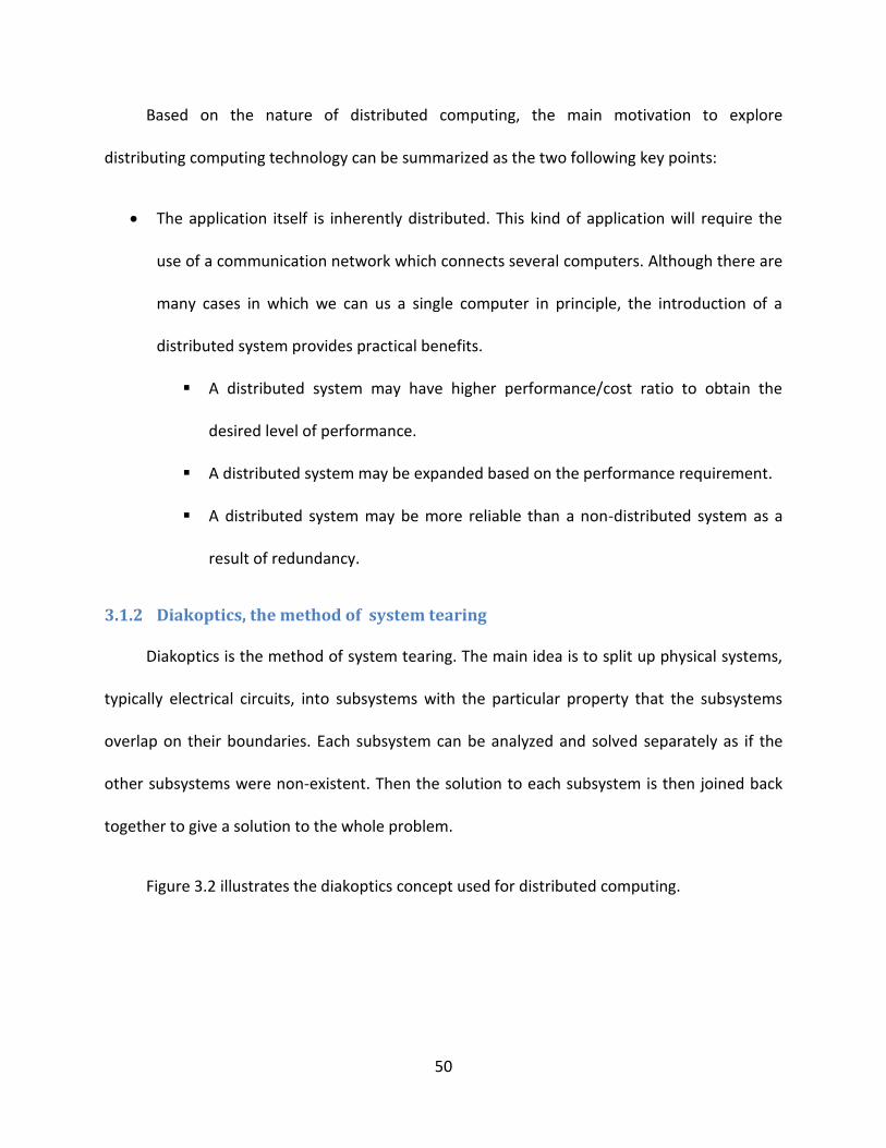
3.1.2 Diakoptics, the method of system tearing

Diakoptics is the method of system tearing. The main idea is to split up physical systems,

typically electrical circuits, into subsystems with the particular property that the subsystems

overlap on their boundaries. Each subsystem can be analyzed and solved separately as if the

other subsystems were non-existent. Then the solution to each subsystem is then joined back

together to give a solution to the whole problem.

Figure 3.2 illustrates the diakoptics concept used for distributed computing.

51

Figure 3.2 Diakoptics for Distributed Computing

3.2 Distributed computing architecture in DEW

Contrasted to the transmission and sub transmission lines which are in a meshed network,

the distribution feeders are usually radial to simplify overcurrent protection [31]. With the

radial configuration of electrical power distribution systems in mind, the DEW system model is

designed to have natural points at which the tearing can occur. These natural points are usually

circuits, voltage sources as well as feeders and cotrees. By taking advantage of Graph Trace

Analysis (GTA) on the model, which will be discussed further in Section 3.2.1, the system can be

separated into independent subsystems naturally, and thus the analysis for the system in

distributed computing can be conducted based on the diakoptics approach.

52

Figure 3.3 shows the distributed computing architecture in DEW. A circuit sever is

responsible for breaking the system into independent circuits and then placing them into a

circuit queue. Feeder performance workers are independent processors which grab

independent circuits in the circuit queue and conduct feeder performance analysis, generating

the independent output reports. Finally, the circuit server collects all of the independent output

reports and combines them into one summary report.

Figure 3.3 Distributed Computing Architecture in DEW

53

3.2.1 Graph Trace Analysis

Graph Trace Analysis (GTA) is a multidiscipline method originally developed at Virginia

Tech for addressing generic analysis with topology iterators, especially electric power systems,

but which has been extended now to other system types [19], [21] and [56].

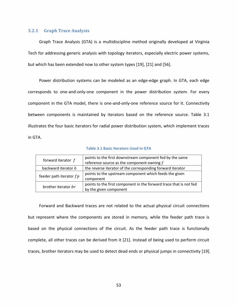
Power distribution systems can be modeled as an edge-edge graph. In GTA, each edge

corresponds to one-and-only-one component in the power distribution system. For every

component in the GTA model, there is one-and-only-one reference source for it. Connectivity

between components is maintained by iterators based on the reference source. Table 3.1

illustrates the four basic iterators for radial power distribution system, which implement traces

in GTA.

Table 3.1 Basic Iterators Used in GTA

forward iterator points to the first downstream component fed by the same reference source as the component owning

backward iterator the reverse iterator of the corresponding forward iterator

feeder path iterator points to the upstream component which feeds the given component

brother iterator points to the first component in the forward trace that is not fed by the given component

Forward and Backward traces are not related to the actual physical circuit connections

but represent where the components are stored in memory, while the feeder path trace is

based on the physical connections of the circuit. As the feeder path trace is functionally

complete, all other traces can be derived from it [21]. Instead of being used to perform circuit

traces, brother iterators may be used to detect dead ends or physical jumps in connectivity [19].

54

Figure3.4 gives an example circuit and Table 3.2 illustrates the four basic iterators for

every component in the example circuit.

Figure 3.4 Sample Circuit for Illustrating GTA [19], [used with permission]

Table 3.2 Iterators for Sample Circuit [19], [used with permission]

Component

1 2 NULL NULL NULL

2 3 1 1 NULL

3 4 2 2 NULL

4 5 3 3 6

5 6 4 4 6

6 7 5 3 NULL

7 8 6 6 13

8 9 7 7 9

9 10 8 7 13

10 11 9 9 11

11 12 10 9 13

12 13 11 11 13

13 14 12 6 NULL

14 NULL 13 13 NULL

55

The four iterators described above are sufficient for the trace algorithms for radial circuits.

For non-radial circuits, adjacent iterators are used to manage and track cotree elements, which

mark an independent loop [17], [19]. This work only discusses the distributed algorithm for

radial power distribution systems. More information on the distributed algorithm for looped

power distribution systems can be found in [45].

The iterator based trace analysis described above enables the “tearing” of independent

circuits from the integrated system model, and thus naturally structures the distributed

computing.

Figure 3.5 Start Componet in DEW

In DEW, for every circuit, there is one component called start-of-circuit which identifies

the start of a separate circuit run, as shown in Figure 3.5. It is the reference for all the

remaining components in that circuit. This provides a natural point to “tear” or separate the

system as shown in Figure 3.6.

56

Figure 3.6 Sample System to Be Separated

Figure 3.7 illustrates the flow chart for dividing the system in DEW into independent

circuits. By locating the starting points of the circuits contained in the system, single circuits are

retrieved by utilizing a forward GTA trace.

57

Figure 3.7 Dividing the System in DEW Flow Chart

3.2.2 GTA Notation for Distributed Algorithm

As the primary focus of GTA is on sets and sequences, [57], a declarative language which

can describe operations on collections, with some minor modifications, is used to describe the

operations of the distributed computing algorithm. Table 3.3 lists the GTA operations used in

the distributed computing algorithm.

58

Table 3.3 GTA Operations Used in Distributed Algorithm

Operation Result Effect

set or seq expr For all elements in , do operation expressed by

seq element The first element of

Set or seq boolean Returns whether there is an element of

element element Assigns to

element Runs feeder performance analysis on

element expr Runs b on a

expr Wait until expr is false

Using GTA, the distributed computing problem can be defined as follows:

A power distribution system to be analyzed by the processor set with distributed

computing, is divided into separate circuits , , … , , … , , which will be uniformly

assigned to available processors for processing by a specified algorithm. The processors

that are busy are placed in the set . Thus,

Formula 3.1 shows the algorithm.

3.1

Figure 3.8 illustrates formula 3.1.

59

Figure 3.8 Distributed Algorithm Flow Chart

3.3 Feeder Performance Analysis with Distributed Algorithm Case Studies

The feeder performance analysis with distributed algorithm case studies is conducted on

the same real-world electrical power distribution system model as shown in Figure 2.5 with

eight identical machines connected in the Gigabit Ethernet LAN at Electrical Distribution Design

Inc as the feeder performance workers and another computer as the circuit server. Tests are

run with 1, 2, 4, and 8 machines.

The distributed computing environment is shown in the photo below.

60

Figure 3.9 Eight machines used for distributed computing

Table 3.4 illustrates the configuration information for the eight feeder performance

workers

Table 3.4 Configuration Information for the Eight Feeder Performance

Workers Used for Distributed Computing

Model Dell Precision T3500

CPU Intel Xeon @2,4GHz

RAM 4G

Table 3.5 illustrates the configuration information for the circuit server

Table 3.5 Configuration Information for the Circuit Server

Model Dell Latitude D630

CPU Intel Core 2 Duo T9300@2,5GHz, 2,49Hz

RAM 3.5G

61

Table 3.6 illustrate the processing time and speed-up for feeder performance analysis

with distributed algorithm

Table 3.6 Processing Time and Speed-Up for Feeder Performance Analysis with Distributed Algorithm

Number of Machines Processing Time (Minutes) Speed UP

1 88 1

2 46 1.913043

4 29 3.034483

8 15 5.866667

Figure 3.10 shows a distributed computing performance plot, which illustrates the

improvements in processing time as the number of computers is increased.

Figure 3.10 Distributed Algorithm Performance Plot

0

15

30

45

60

75

90

0 2 4 6 8

Processing Time

(Minutes)

Number of the Computers

Distributed Algorithm Performance Plot

Processing Time

62

The following observations can be concluded from Table 3.6 and Figure 3.10:

The processing time is significantly decreased and thus the overall performance is

effectively improved.

The overall running time is approximately linearly scaled down. However,

performance analysis itself could not be parallelized in the algorithm proposed in

this thesis for every single feeder, the linear scalability holds only when the quantity

of feeder needed to be analyzed significantly surpass the available amount of

computers.

Overhead exists as a result of communication between circuit server and feeder

performance workers

As the overall running time is affected by computation time and communication

time and it is roughly linearly scaled down, it can be concluded that the computation

time dominates the communication overhead time.

63

CHAPTER 4 Conclusions and Future Work

4.1 Conclusion

This thesis investigates feeder performance analysis of electric power distribution

systems with distributed algorithm. To the best of the author’s knowledge, it is the first time

that this detailed performance analysis is researched, developed and tested, using a diakoptics

based tearing method and Graph Trace Analysis (GTA) to split the system so that it can be

analyzed with distributed computing technology.

The main contributions of this work are summarized as follows:

Detailed feeder performance analysis of electric power distribution system is

conducted with case studies on real world systems.

Built up on DEW, Power flow analysis, and LMP analysis as the groundwork,

feeder performance analysis of electric power distribution system computes a

modeled circuit’s performance over an entire year, listing key circuit

performance parameters such as efficiency, loading, losses, cost impact, power

factor, three phase imbalance, and capacity usage, providing detailed operating

information of the system.

By analyzing the whole system, it provides an overall view of the performance of

every circuit in the system, providing the ability to target the inefficient circuits,

three phase imbalance or cost impact and others.

64

Real time Locational Marginal Price (LMP) is used to evaluate the cost

LMP analysis is implemented to convert non-standard LMP data to standard data. By

incorporating standard LMP data with feeder performance analysis, the performance of circuits

is accurately measured with concrete cost.

Distributed computation technology is utilized to speed up the computation

Based on a diakoptics tearing method and Graph Trace Analysis, a distributed computing

architecture is proposed. The distributed computing algorithm is described with Graph Trace

Analysis. The performance improvement is demonstrated through a real world system case

study.

4.2 Future Work

The following work is recommended as possible future improvements:

A performance based planning tool may be researched and developed based upon

feeder performance analysis.

Performance analysis can help planners to target the best design from among many

feasible designs that might work for their system by simulating the plan first on computer. It is

not only meaningful but also practical to have a planning tool researched and designed based

on feeder performance analysis presented in this work.

65

The distributed computing architecture may be extended to other analysis.

As the distributed computing architecture proposed in this work is a general one, it is

possible to extend it to other analysis of electrical power distribution systems other than feeder

performance analysis.

66

References

[1]J.D.Glover, M.S.Sarma , T.J.Overbye, “Power System Analysis and Design”, Foruth Edition,

Cengage Learning

[2]T.Gonen, “Electric Power Distribution System Engineering”, Second Edition, CRC Press

[3]H.L.Willis, “Power Distribution Planning Reference Book”, Second Edition, MARCEL DEKKER,

INC.

[4]H.L.Willis, H.Tram, M.V.Engel, L.Finley, “Optimization applications to power distribution”,

IEEE Transactions on Computer Applications in Power, Vol.8, Iss.4, pp.12-17, Oct, 1995

[5]I. P. E. Society, "Smart Distribution Grid and the Advanced Integrated Distribution

Management Systems (IDMS)," in PSCE Tutorial, Seattle, Washington, 2009.

[6]Y. Liang, K.S. Tam, R. Broadwater, “Load Calibration and Model Validation Methodologies for

Power Distribution Systems”, IEEE Transactions on Power Systems, Vol.25, Iss.3, Aug, 2010

*7+M. Baran, "Challenges in distribution system analysis”, IEEE Power Engineering Society

Summer Meeting, vol.2, pp. 627, 1999

[8]H. Brown, S. Suryanarayanan, “A survey seeking a definition of a smart distribution system,”

IEEE North American Power Symposium (NAPS), Starkville, MS, 2009

67

[9]New York Independent System Operator, http://www.nyiso.com/public/index.jsp, (accessed

Oct. 29, 2010

[10]Midwest ISO, http://www.midwestmarket.org/page/LMP+Contour+Map+(EOR), (accessed

Oct. 29, 2010)

[11]H.E. Shaalan, J. Thompson, R. Broadwater, H. Ng , “DEWorkstation: a comprehensive

distribution modeling tool” , IEEE Transmission and Distribution Conference, 1996

[12]H.E. Shaalan, J. Thompson, R. Broadwater, M. Ellis, H. Ng , “Distribution engineering tool

features a flexible framework” IEEE Transctions on Computer Applications in Power, Vol.8, Iss.3,

1995

[13]M.Dilet, R.P.Broadwater, “An introduction to integrated design in electrical distribution”,

IEEE Power Engineering Society Winter Meeting, Vol.2, pp.991-994, 2002.

[14]F. Li, R. Broadwater, “Software Framework Concepts for Power Distribution System

Analysis,” IEEE Transactions on Power Systems, Vol. 19, No. 2, pp. 948-956, May, 2004.

[15]J.Hambrick, R. Broadwater, “Configurable, Hierarchical, Model-based Control of Electrical

Distribution Circuits,” IEEE Transactions on Power Systems, 2010.

[16]H.Shaalan, J.Thompson, R.Broadwatre, M.Ellis and H.Ng, “Distribution Engineering Tool

Features a Flexible Framework” IEEE Computer Applications in Power, Vol. 8, No. 3, pp. 21-24,

July, 1995

68

[17]R. Broadwater, J. Thompson, M. Ellis, H. Ng, N. Singh, D. Lloyd, “Application Programmer

Interface For The EPRI Distribution Engineering Workstation,” IEEE Transactions on Power

Systems, Vol. 10, No. 1, pp. 499-505, February, 1995.

[18]R. Broadwater, M.Dilet, J. Thompson, D. Lloyd, “Design of integrated software for

reconfiguration, reliability, and protection system analysis”, IEEE/PES Transmission and

Distribution Conference and Exposition, 2001

[19]R.Broadwate, J.Thompson, and T.E. McDermott, “Pointers and linked lists in electric power

distribution circuit analysis.’’ IEEE Power Industry Computer Application Conference, pp. 16–2,

1991

[20]L.R. Feinauer, M. E. Ison, R. Broadwater, “Generic Algorithms for Analysis of Interdependent

Multi-Domain Network Systems,” International Journal on Critical Infrastructures, Vol. 6, No.

1,pp. 81-95. 2010

*21+L.R. Feinauer, K.J.Russell, R. Broadwater, “Graph Trace Analysis and Generic Algorithms for

Interdependent Reconfigurable System Design and Control“, Naval Engineers Journal, Vol.120,

Iss.1, 2008.

[22]A. Sargent, R. Broadwater, J.C.Thompson, J. Nazarko, “ Estimation of diversity and kWHR-

to-peak-kW factors from load research data”, IEEE Transactions on Power Systems, Vol. 9, Iss. 3,

pp. 1450-1456, Aug, 1994

69

*23+F.Li, R.Broadwater, A.Sargent, ”Cable impedance calculations with parallel circuits and

multi-neutral returns in distribution networks” IEEE Power Engineering Society Winter Meeting,

2001.

[24]M. Dilek, F.D.Leon, R.Broadwater, S. Lee, “A Robust Multiphase Power Flow for General

Distribution Networks”, IEEE Transactions on Power Systems, Vol. 25, No.2, pp.760-768, May,

2010

[25]M. Dilek, R. Broadwater, R. Sequin, "Computing Distribution System Fault Currents and

Voltages via Numerically Computed Thevenin Equivalents and Sensitivity Matrices," IEEE Power

Systems Conference and Exposition, October, 2004

[26]D. Zhu, R. Broadwater, K. Tam, R. Seguin, and H. Asgeirsson, “Impact of DG placement on

reliability and efficiency with time-varying loads,” IEEE Transactions on Power Systems., Vol. 21,

No. 1, pp. 419-427, Feb, 2006.

[27]R. Broadwater, H. E. Shaalan, A.Oka, R. Lee, “Distribution system reliability and restoration

analysis”, Electric Power System Research, pp. 203-211, 1994.

[28]M. Dilek, R. Broadwater, R. Sequin,” Phase prediction in distribution systems”, IEEE Power

Engineering Society Winter Meeting, 2002.

[29]D. Kleppinger, R. Broadwater, C. Scirbona, “Generic Reconfiguration for Restoration,”

Electric Power Systems Research Journal, Vol. 80, Iss. 3, pp.287-295, March, 2010

70

[30]I.Drezga, R.Broadwater, A.J.Sugg, “Object-oriented analysis of distribution system

reconfiguration for power restoration “, IEEE Power Engineering Society Summer Meeting, 2001.

*31+T.E.Mcdermott, I.Drezga, R.Broadwater, ” A heuristic nonlinear constructive method for

distribution system reconfiguration”, IEEE Transactions on Power Systems, Vol.14, Iss.2, pp.

478-483, May, 1999

[32]M. Dilek, R. Broadwater, J. Thompson, R. Sequin, “Simultaneous Phase Balancing at

Substations and Switches with Time-Varying Load Patterns”, IEEE Transactions on Power

Systems, Vol. 16, No. 4, pp. 922-928, Nov, 2001

[33]M. Dilek, “Integrated Design of Electrical Distribution Systems: Phase Balancing and Phase

Prediction Case Studies” , Ph.D. Dissertation, Electrical and Computer Engineering Department,

Virginia Polytechnic Institute and State University, Blacksburg, VA, 2001

[34]Y. Y. Hsu, H. C. Kuo, “Dispatch of capacitors on distribution system using dynamic

programming”, IEEE Proceedings in Generation, Transmission and Distribution, Vol. 140, Iss. 6,

pp. 433–438, Nov, 1993.

[35]J.Teng, C.Chen, C.Chen, Y.Liu, “Optimal capacitor control for unbalanced distribution

systems with distributed generations,” in IEEE International Conference on Sustainable Energy

Technologies, 2008

[36]W.H.Kersting, “Distribution System Modeling and Analysis”, Second Edition, CRC Press

71

[37]E.W. Dijkstra, "Solution of a problem in concurrent programming control", Communications

of the ACM , Vol.5, Nom.9, September, 1965

[38]PODC Influential Paper Award: 2002, http://www.podc.org/influential/2002.html,

(accessed April. 25, 2010)

*39+M.Crummey, M. L.Scotty: “Algorithms for scalable synchronization on shared-memory

multiprocessors” ACM Transactions on Computer Systems, Vol 9, No. 1, , pp. 21-65, February,

1991

[40]Edsger W. Dijkstra Prize in Distributed Computing: 2006,

http://www.podc.org/dijkstra/2006.html, (accessed April. 25, 2010)

[41]M.Pease, R. Shostak, L.Lamport, "Reaching agreement in the presence of faults", Journal of

the Association for Computing Machinery, Vol. 27, No. 2, pp 228-234, April, 1980

[42]L.Lamport, R.Shostak, M.Pease, "The Byzantine generals problem", ACM Transactions on

Programming Languages and Systems, Vol. 4, No. 3, pp. 382-401, July, 1982

[43]M.Fische, N.Lynch, M.Paterson, "Impossibility of distributed consensus with one faulty

process" Journal of the Association for Computing Machinery, Vol. 32, No. 2, pp. 374-382, April,

1985,

[44]C. Dwork, N.Lynch, L. Stockmeyer, "Consensus in the presence of partial synchrony",

Journal of the Association for Computing Machinery, Vol. 35, No. 2, pp. 288-323, April, 1988

72

*45+F. Li, R.Broadwater, “Distributed algorithms with theoretic scalability analysis of radial and

looped load flows for power distribution systems”, Electrical Power System Research, Vol. 65,

Iss.2, pp.169-177, March, 2003

[46]J.R. Santos, A.G. Exposito, J.L.M. Ramos, “Distributed contingency analysis: practical issues”,

IEEE Transactions on Power Systems”, Vol. 14 Iss.4, pp.1349-1354, 1999

[47]G. Kron, "Diakoptics: The Piecewise Solution of Large Scale Systems", MacDonald, 1963

[48]H.H.Happ, “Diakoptics—The solution of system problems by tearing” Proceedings of the

IEEE”, Vol.62, Iss.7, 1974

[49]C.H.Lai , "Diakoptics, Domain Decomposition and Parallel Computing", The Computer

Journal, Vol 37, No, 10, pp. 840-846, 1994

[50]“Locational Marginal Pricing (LMP): Basics of Nodal Price Calculation”,

http://www.caiso.com/docs/2004/02/13/200402131607358643.pdf, (accessed Feb. 1, 2011)

[51]E. Litvinov, “Power System & LMP Fundamentals”, ISO New England Inc., 2006

[52]P. Springs, “Economic Dispatch: Concepts, Practices and Issues”, Presentation to the Joint

Board for the Study of Economic Dispatch, 2005

[53]W. W. Hogan, “Electricity market design: Coordination, Pricing and Incentives”, Conference

on the Economics of Energy Markets, June, 2008

73

[54]Search for Extraterrestrial Intelligence (SETI), http://setiathome.berkeley.edu/, (accessed

April. 21, 2010)

[55]Cornell CS 414 Operating System Class Website,

http://www.cs.cornell.edu/Courses/cs414/2004su/slides/18_distributed.pdf, (accessed April.

21, 2010)

[56]D.L. Kleppinger, K.J. Russell, and R.Broadwater, “Graph trace analysis based shipboard

HM&E system priority management and recovery analysis,’’ IEEE Electric Ship Technologies

Symposium, May 2007, pp. 109–114.

[57]J. Warmer and A. Kleppe, “Object Constraint Language, The: Getting Your Models Ready for

MDA”. Second Edition, Addison-Wesley Professional, 2003.