FEEDBACK STABILIZATION METHODS FOR THE …iasonkar/paper38.pdfFEEDBACK STABILIZATION METHODS FOR ODE...
35
DISCRETE AND CONTINUOUS doi:10.3934/dcdsb.2011.16.283 DYNAMICAL SYSTEMS SERIES B Volume 16, Number 1, July 2011 pp. 283–317 FEEDBACK STABILIZATION METHODS FOR THE NUMERICAL SOLUTION OF ORDINARY DIFFERENTIAL EQUATIONS Iasson Karafyllis Department of Environmental Engineering Technical University of Crete 73100 Chania, Greece Lars Gr¨ une Mathematical Institute University of Bayreuth 95440 Bayreuth, Germany (Communicated by Peter E. Kloeden) Abstract. In this work we study the problem of step size selection for numer- ical schemes, which guarantees that the numerical solution presents the same qualitative behavior as the original system of ordinary differential equations. We apply tools from nonlinear control theory, specifically Lyapunov function and small-gain based feedback stabilization methods for systems with a glob- ally asymptotically stable equilibrium point. Proceeding this way, we derive conditions under which the step size selection problem is solvable (including a nonlinear generalization of the well-known A-stability property for the implicit Euler scheme) as well as step size selection strategies for several applications. 1. Introduction. It is well-known that step size control can enhance the perfor- mance of numerical schemes for solving ordinary differential equations (ODEs). In fact, the use of the word “control” suggests that methods and techniques from math- ematical control theory can in principle be used in order to achieve certain objectives for the numerical solution. For example, in [16] the authors use a “Proportional- Integral” technique which is similar to the “Proportional-Integral” controller used in Linear Systems Theory in order to keep the local discretization error within certain bounds, see also [14, 15, 19]. Theoretical results on the behavior of adaptive time stepping methods have been presented in [27, 29] and the control theoretic notion of input-to-state stability (ISS) has been successfully used in [11, 12] in order to explain the behavior of attractors under discretization. In this work, we develop tools for numerical schemes which are similar to methods used in nonlinear control theory. We consider the problem of selecting the step size for numerical schemes so that the numerical solution presents the same qualitative behavior as the original nonlinear ODE. It is well-known that any consistent and stable numerical scheme for ODEs inherits the asymptotic stability of the original equation in a practical sense, even for more general attractors than equilibria, see 2000 Mathematics Subject Classification. Primary: 65L07, 34D20; Secondary: 65L06, 93D15. Key words and phrases. Asymptotic stability of numerical approximations, feedback stabiliza- tion, nonlinear differential equations. 283
Transcript of FEEDBACK STABILIZATION METHODS FOR THE …iasonkar/paper38.pdfFEEDBACK STABILIZATION METHODS FOR ODE...

DISCRETE AND CONTINUOUS doi:10.3934/dcdsb.2011.16.283DYNAMICAL SYSTEMS SERIES BVolume 16, Number 1, July 2011 pp. 283–317
FEEDBACK STABILIZATION METHODS FOR THE
NUMERICAL SOLUTION OF ORDINARY
DIFFERENTIAL EQUATIONS
Iasson Karafyllis
Department of Environmental Engineering
Technical University of Crete
73100 Chania, Greece
Lars Grune
Mathematical Institute
University of Bayreuth95440 Bayreuth, Germany
(Communicated by Peter E. Kloeden)
Abstract. In this work we study the problem of step size selection for numer-ical schemes, which guarantees that the numerical solution presents the same
qualitative behavior as the original system of ordinary differential equations.
We apply tools from nonlinear control theory, specifically Lyapunov functionand small-gain based feedback stabilization methods for systems with a glob-
ally asymptotically stable equilibrium point. Proceeding this way, we derive
conditions under which the step size selection problem is solvable (including anonlinear generalization of the well-known A-stability property for the implicit
Euler scheme) as well as step size selection strategies for several applications.
1. Introduction. It is well-known that step size control can enhance the perfor-mance of numerical schemes for solving ordinary differential equations (ODEs). Infact, the use of the word “control” suggests that methods and techniques from math-ematical control theory can in principle be used in order to achieve certain objectivesfor the numerical solution. For example, in [16] the authors use a “Proportional-Integral” technique which is similar to the “Proportional-Integral” controller used inLinear Systems Theory in order to keep the local discretization error within certainbounds, see also [14, 15, 19]. Theoretical results on the behavior of adaptive timestepping methods have been presented in [27, 29] and the control theoretic notionof input-to-state stability (ISS) has been successfully used in [11, 12] in order toexplain the behavior of attractors under discretization.
In this work, we develop tools for numerical schemes which are similar to methodsused in nonlinear control theory. We consider the problem of selecting the step sizefor numerical schemes so that the numerical solution presents the same qualitativebehavior as the original nonlinear ODE. It is well-known that any consistent andstable numerical scheme for ODEs inherits the asymptotic stability of the originalequation in a practical sense, even for more general attractors than equilibria, see
2000 Mathematics Subject Classification. Primary: 65L07, 34D20; Secondary: 65L06, 93D15.Key words and phrases. Asymptotic stability of numerical approximations, feedback stabiliza-
tion, nonlinear differential equations.
283
284 IASSON KARAFYLLIS AND LARS GRUNE
for instance [11, 12, 26] and [35, Chapter 7] for fixed step size and [5, 27] forschemes with variable step size. Practical asymptotic stability means that thesystem exhibits an asymptotically stable set close to the original attractor, i.e., inour case a small neighbourhood around the equilibrium point, which shrinks down tothe attractor as the time step h tends to 0. In contrast to these results, in this paperwe investigate the case in which the numerical approximation is asymptoticallystable in the usual sense, i.e., not only practically.
Here, we concentrate on nonlinear systems for which an equilibrium point is theglobal attractor. In Section 2 of the present work it is shown how the problemof appropriate step size selection can be converted to a rigorous abstract feedbackstabilization problem for a particular hybrid system. The idea of representing nu-merical schemes as hybrid systems goes back to [22] and the reader should noticethat the standard stability analysis of numerical schemes uses discrete-time system,see, e.g., [19, 17, 21, 28, 35], rather than hybrid systems. With this approach, weare in the position to use all methods of feedback design for nonlinear systems.Specifically, we consider methods based on small-gain theorems and methods basedon Lyapunov functions.
Both methods have been used widely in nonlinear systems theory for the solu-tion of feedback stabilization problems, see [1, 4, 20, 23, 25, 33, 34] and referencestherein. In the present work, the above methods are used for the step size selectionfor numerical schemes for ODEs, see Section 3 and Section 4. While the small-gainmethod allows for the design of novel numerical schemes for nonlinear systems withspecific structures, cf. Theorem 3.1 and Theorem 3.3, the Lyapunov function basedmethod allows for results for general nonlinear systems. It applies to arbitrary con-sistent Runge-Kutta schemes (see Theorem 4.5, Theorem 4.9 and Theorem 4.12) aswell as to specific Runge-Kutta schemes, see Corollary 4.7 and Theorem 4.17. Someof our results constitute nonlinear extensions of well-known properties of numericalschemes like, e.g., A-stability, cf. Corollary 4.18. While the idea behind this Lya-punov based approach is conceptually similar to the geometric integration methodrecently proposed in [10], our methodology relies on the appropriate selection of thetime step rather than on the modification of the numerical scheme.
The key idea used in small-gain approach is to formulate numerical schemesin such a way that small-gain criteria from the hybrid control systems literaturebecome applicable. These criteria then induce an upper bound on the time stepfor which stability of the numerically computed solutions can be guaranteed. Inthe Lyapunov based approach, the basic idea is to use a Lyapunov function for thecontinuous time system as a Lyapunov function for the numerical approximation,which in turn implies the desired stability property by Lemma 4.1. Conditionsunder which this is possible and corresponding bounds on the time step are derivedeither from estimates on the discretization error as in Theorem 4.5, Theorem 4.9and Theorem 4.12, or from structural properties of the scheme and the Lyapunovfunction as in Theorem 4.17.
A number of applications of the obtained results is developed in Sections 5 and6. For instance, in Section 6 we consider the possibility of using explicit schemesfor stiff linear systems of ODEs. An application of the stabilization method basedon the small-gain analysis for systems described by partial differential equations(PDEs) is presented in Section 5.
Thus, the contribution of the paper is twofold. On the one hand, our control theo-retic approach yields new insight into the stability properties of numerical schemes
FEEDBACK STABILIZATION METHODS FOR ODE NUMERICS 285
and as such it adds another means to the toolbox for stability investigations ofnumerical schemes. On the other hand, our method leads to the design of newdiscretization schemes and step size control algorithms, which instead of the usualcontrol of the local discretization error take care of the global qualitative behaviour.
Notation Throughout this paper we adopt the following notation:Let A ⊆ Rn be a set. By C0(I ; Ω), we denote the class of continuous functions
on I, which take values in Ω. By Ck(I ; Ω), where k ≥ 1 is an integer, we denotethe class of differentiable functions on A with continuous derivatives up to orderk, which take values in Ω. By C∞(A; Ω), we denote the class of differentiablefunctions on A having continuous derivatives of all orders, which take values in Ω,i.e., C∞(A; Ω) =
⋂k≥1 C
k(A; Ω).
For a vector x ∈ Rn we denote by |x| its usual Euclidean norm and by x′ itstranspose. By Bε(x), where ε > 0 and x ∈ Rn, we denote the ball of radius ε > 0centered at x ∈ Rn, i.e., Bε(x) := y ∈ Rn : |y − x| < ε . For a real matrix A ∈Rn×m we denote by |A| its induced norm, i.e., |A| := max |Ax| : x ∈ Rm , |x| = 1 and by A′ ∈ Rm×n its transpose.
R+ denotes the set of non-negative real numbers and Z+ the set of non-negativeinteger numbers. C denotes the set of complex numbers. By K∞ we denote theset of all increasing and continuous functions ρ : R+ → R+ with ρ(0) = 0 andlims→+∞ ρ(s) = +∞.
For every scalar continuously differentiable function V : Rn → R, ∇V (x) denotesthe gradient of V at x ∈ Rn, i.e., ∇V (x) = ( ∂ V∂x1
(x), . . . , ∂ V∂xn (x)). We say that a
function V : Rn → R+ is positive definite if V (x) > 0 for all x 6= 0 and V (0) = 0.We say that a continuous function V : Rn → R+ is radially unbounded if for everyM > 0 the set x ∈ Rn : V (x) ≤M is compact.
For a sufficiently smooth function V : Rn → R we denote by LfV (x) :=
∇V (x)f(x) the Lie derivative of V along f and we define recursively L(i+1)f V (x) =
Lf (L(i)f V (x)) for i ≥ 1.
2. Setup, preliminaries and problem formulation. Consider the autonomoussystem
z(t) = f(z(t)) , z(t) ∈ Rn (1)
where f : Rn → Rn is a locally Lipschitz vector field with f(0) = 0. For everyz0 ∈ Rn and t ≥ 0, the solution of (1) with initial condition z(0) = z0 will bedenoted by z(t, z0).
There are several ways of formalizing numerical approximations of system (1)with varying step-sizes as dynamical systems. In this paper we will use hybridsystems for this purpose. After introducing this class of systems, establishing itsrelation to numerical schemes and deriving some of its properties, we will discussin Remark 2.1 why we prefer to use this formulation. The hybrid system we areconsidering is given by
x(t) = F (hi, x(τi)) , t ∈ [τi, τi+1)
τ0 = 0 , τi+1 = τi + hi
hi = ϕ(x(τi)) exp(−u(τi))
x(t) ∈ Rn , u(t) ∈ [0,+∞)
(2)
286 IASSON KARAFYLLIS AND LARS GRUNE
where ϕ ∈ C0(Rn; (0, r]), r > 0 is a constant, F :⋃x∈Rn ([0, ϕ(x)]× x) → Rn
is a (not necessarily continuous) vector field with F (h, 0) = 0 for all h ∈ [0, ϕ(0)],limh→0+ F (h, z) = f(z), for all z ∈ Rn. More specifically, the solution x(t) of thehybrid system (2) is obtained for every locally bounded u : R+ → R+ and x0 ∈ Rnby setting τ0 = 0, x(0) := x0 and then proceeding iteratively for i = 0, 1, . . . asfollows (cf. [22]):
(i) Given τi and x(τi), calculate τi+1 according to τi+1 = τi+ϕ(x(τi)) exp(−u(τi))(ii) Compute the state trajectory x(t), t ∈ (τi, τi+1] as the solution of the differ-
ential equation x(t) = F (hi, x(τi)), i.e., x(t) = x(τi) + (t− τi)F (hi, x(τi)) fort ∈ (τi, τi+1].
We denote the resulting trajectory by x(t, x0, u) or briefly x(t) when x0 and u areclear from the context.
We will further assume that there exists a continuous, non-decreasing functionM : R+ → R+ such that
|F (h, x)| ≤ |x|M (|x|) for all x ∈ Rn and h ∈ [0, ϕ(x)] (3)
It should be noticed that the hybrid system (2) under hypothesis (3) is an au-tonomous system, which satisfies the “Boundedness-Implies-Continuation” prop-erty and for each locally bounded input u : R+ → R+ and x0 ∈ Rn there existsa unique absolutely continuous function [0,+∞) 3 t → x(t) ∈ Rn with x(0) = x0
which satisfies (2), see [22]. Some remarks are needed in order to explain the name“numerical approximation of system (1)” for the hybrid system (2).
(i) The condition limh→0+ F (h, z) = f(z) is the usual consistency condition forthe numerical scheme applied to (1).
(ii) The sequence hi∞0 is the sequence of step sizes used in order to obtainthe numerical solution. Notice that for the case ϕ(x) ≡ r, constant inputsu(t) ≡ u ≥ 0 will produce constant step sizes with hi ≡ r exp(−u). Arbitraryvariable step size sequences hi ∈ (0, ϕ(x(τi)] can be represented easily byselecting appropriate inputs u : R+ → R+.
(iii) The constant r > 0 is the maximal allowable step size.(iv) The function ϕ ∈ C0(Rn; (0, r]) determines the maximum allowable step size
ϕ(x(τi)) for each x(τi) ∈ Rn. This is important for implicit numerical schemesas shown below.
All consistent s-stage Runge-Kutta methods can be represented by the hybrid sys-tem (2). More specifically, let x0 ∈ Rn and consider a consistent s-stage Runge-Kutta method for (1):
Yi = x0 + h
s∑j=1
aijf(Yj), i = 1, . . . , s (4)
x = x0 + h
s∑i=1
bif(Yi) (5)
with∑si=1 bi = 1. If the scheme is explicit, i.e., if aij = 0 for j ≥ i, then there
always exists a unique solution to equations (4). If the scheme is implicit, then inorder to be able to guarantee that equations (4) admit a unique solution it may benecessary to restrict the step size to h ∈ [0, ϕ(x0)] for some maximal step size ϕ(x0)
FEEDBACK STABILIZATION METHODS FOR ODE NUMERICS 287
depending on the state x0 ∈ Rn. In all subsequent statements on implicit schemes,we will tacitly assume that such a step size restriction is imposed if necessary.
A suitable choice for ϕ(x) may be obtained in the following way. Let γ : R+ → R+
be a continuous, non-decreasing function with |f(x)| ≤ |x| γ (|x|) for all x ∈ Rn(such a function always exists since f : Rn → Rn is a locally Lipschitz vec-tor field with f(0) = 0). Let Lλ : Rn → (0,+∞) be a continuous function
with Lλ(x0) ≥ sup|f(x)−f(y)||x−y| : x, y ∈ Nλ(x0) , x 6= y
for all x0 ∈ (Rn\0),
with Nλ(x0) := x ∈ Rn : |x− x0| ≤ λ |x0| , λ ∈ (0, 1). The continuous func-tion ϕ(x) := λ
|A| (Lλ(x)+γ(|x|)) , where |A| := maxi=1,...,s
∑sj |aij |, guarantees that for
all x0 ∈ Rn and h ∈ [0, ϕ(x0)] the equations (4) have a unique solution satisfyingYi ∈ Nλ(x0), i = 1, . . . , s.
Note, however, that this bound may be conservative. For instance, we may applythe implicit Euler scheme (s = 1, a11 = b1 = 1) to an asymptotically stable linearODE of the form x = Qx with a matrix Q ∈ Rn×n, i.e., all eigenvalues of Q havenegative real part. Then (4) becomes
Y1 = x0 + hQY1 ⇔ (I − hQ)Y1 = x0
which always has a unique solution because all eigenvalues of −Q and thus of I−hQhave positive real parts for all h ≥ 0; hence I − hQ is invertible for all h ≥ 0.
In order to obtain the hybrid system (2) from (4), (5), we define
F (h, x0) := h−1 (x− x0) =
s∑i=1
bif(Yi) (6)
A moment’s thought reveals that for every locally bounded u : R+ → R+ andx0 ∈ Rn the solution of (2) with (6) coincides at each τi, i ≥ 0 with the numericalsolution of (1) with x(0) = x0 obtained by using the Runge-Kutta numerical scheme(4), (5) and using the discretization step sizes hi = ϕ(x(τi)) exp(−u(τi)), i ≥ 0. Thereader should notice that other ways (besides (6)) of defining the vector field F :⋃x∈Rn ([0, ϕ(x)]× x) → Rn may be possible; here we have selected the simplest
way of obtaining a piecewise linear numerical solution.Appropriate step size restriction can always guarantee that (3) holds for F from
(6). For example, if ϕ(x) := λ|A| (Lλ(x)+γ(|x|)) is the step size restriction described
above, then for all x ∈ Rn and h ∈ [0, ϕ(x)] the function F from (6) satisfies
|F (h, x)| ≤ |x|
[1 + r(1 + λ)
(s∑i=1
|bi|
)γ ((1 + λ) |x|)
].
Thus, (3) holds with M(y) := 1 + r(1 + λ) (∑si=1 |bi|) γ ((1 + λ)y).
Before we turn to the problem formulation, we collect some further estimates onRunge-Kutta schemes which will be useful in the following sections.
If the Runge-Kutta scheme (4), (5) is of order p ≥ 1, we will occasionally furtherassume that f ∈ Cp(Rn;Rn) and for each fixed x ∈ Rn the mapping [0, ϕ(x)] 3h→ F (h, x) is p times continuously differentiable with
|F (h, x)|+p∑j=1
∣∣∣∣ ∂j∂ hjF (h, x)
∣∣∣∣≤ G (|x|) max |f(y)| : y ∈ Rn , |y − x| ≤ |x|ϕ(x)M(|x|)
(7)
for all x ∈ Rn and h ∈ [0, ϕ(x)] and some continuous, non-decreasing functionG : R+ → R+, where M : R+ → R+ is the function involved in (3). Again,

288 IASSON KARAFYLLIS AND LARS GRUNE
appropriate step size restriction can always guarantee that (7) holds for F from(6). Notice that the implicit function theorem for (4) guarantees for each fixedx ∈ Rn the existence of ϕ(x) > 0 such that the mapping [0, ϕ(x)] 3 h → F (h, x)is p times continuously differentiable. A suitable choice for ϕ(x) may be obtainedby the formula ϕ(x) := λ
1+2|A|max |Df(z)| : |z|≤(1+λ)|x| , where λ ∈ (0, 1), |A| :=
maxi=1,...,s
∑sj |aij |. However, again this step size restriction may be conservative,
e.g., for explicit schemes.Using Theorem II.3.1 in [18], (7), the fact that f ∈ Cp(Rn;Rn) and the fact that
gk(z(h, x)) = ∂k
∂ hkz(h, x) for k ≥ 1, where gk : Rn → Rn for k = 1, . . . , p + 1 are
vector fields obtained by the recursive formulae g1(z) = f(z), gi+1(z) = Dgi(z)f(z),we may conclude that there exist continuous functions N : Rn → (0,+∞), C : Rn →R+ such that the inequalities
C(x) ≤ N (x)[
max |f(y)| : y ∈ Rn , |y − x| ≤ |x|ϕ(x)M(|x|)
+ max |f(z(h, x))| : h ∈ [0, ϕ(x)] ] (8)
and|z(h, x)− x− hF (h, x)| ≤ hp+1C(x) (9)
hold for all x ∈ Rn and h ∈ [0, ϕ(x)].If we further assume that there exists a neighborhood N ⊆ Rn with 0 ∈ N
satisfying
(i) there exists a constant Λ > 0 and an integer q ≥ 1 such that |f(x)| ≤ Λ |x|qfor all x ∈ N
(ii) there exists a constant Q > 0 such that |z(h, x)| ≤ Q |x| for all x ∈ N andh ∈ [0, ϕ(x)]
then it follows from (8) that there exists a neighborhood N ⊆ N with 0 ∈ N anda constant K > 0 such that
C(x) ≤ K |x|q for all x ∈ N . (10)
Remark 2.1. Modelling numerical schemes as hybrid systems is nonstandard sinceusually numerical approximations are represented as discrete time dynamical sys-tems. In this context, varying time steps can either be handled as part of anextended state space, cf. [29], or by defining the discrete time system on the nonuni-form time grid τ0, τ1, τ2, . . . induced by the time steps, cf. [27] or [5]. In particular,the formulation in [5] in which the time steps hi are included as additional argu-ments in the solution maps is very similar to our approach and we conjecture thatwith this setting one could obtain similar results as in this paper. Still, we believethat for our purposes hybrid systems have some advantages over the alternativediscrete time approaches as summarized in the following points.
(i) In our problem formulation, below, we aim at stability statements for allstep size sequences (hi)i∈N0 with hi > 0 and hi ≤ ϕ(x(τi)), cf. the discussion afterDefinition 2.3. Once ϕ is fixed, for the hybrid system (2) this is equivalent toensuring the desired stability property for all locally bounded functions u : R+ →R+. Hence, our hybrid approach leads to an explicit condition (“for all u”) whilethe discrete time approach leads to a more technical implicit condition (“for all hisatisfying hi ≤ ϕ(x(τi))”).
(ii) The interpolation of the solution in between the grid points τi as inducedby the definition of F in (6) does not complicate our analysis. Indeed, it is wellknown that any meaningful interpolation of numerical solutions does not change
FEEDBACK STABILIZATION METHODS FOR ODE NUMERICS 289
the stability behavior of the resulting solution. We have decided to include theinterpolation in order to make our definition of hybrid systems compatible with theliterature we are using. While on the one hand this makes the definition of thenumerical approximation somewhat more technical, on the other hand we do nothave to keep track of the grid points τn or time steps hi in formulating our resultswhich enhances the readability of these statements.
(iii) Last but not least, the formulation via hybrid models enables us to usereadily available stability results from the hybrid control systems literature, whilefor other formulations we would have to rely on ad hoc arguments in several placesin this paper.
Let us now turn to the formulation of the problem we will consider in this paper.We assume that (1) satisfies the following property, cf. [30] (see also [22, 25]).
Definition 2.2. We say that the origin 0 ∈ Rn is uniformly globally asymptoticallystable (UGAS) for (1) if it is
(i) Lyapunov stable, i.e., for each ε > 0 there exists δ > 0 such that |z(t, z0)| ≤ εfor all t ≥ 0 and all z0 ∈ Rn with |z0| ≤ δ and
(ii) uniformly attractive, i.e., for each R > 0 and ε > 0 there exists T > 0 suchthat |z(t, z0)| ≤ ε for all t ≥ T and all z0 ∈ Rn with |z0| ≤ R.
Furthermore, we say that 0 ∈ Rn is locally exponentially stable if there existsC > 0, σ > 0 and δ > 0 such that |z(t, z0)| ≤ C exp(−σt)|z0| holds for all t ≥ 0 andall z0 ∈ Rn with |z0| ≤ δ.
Given an ordinary differential equation (1) for which the origin is UGAS, our goalis to be able to produce numerical solutions which inherit this qualitative property.That is, we would like to know a continuous function ϕ : Rn → (0, r] such thatthe numerical solution produced by (2) has the correct qualitative behavior, i.e.,that x(t, x0, u) (instead of z(t, z0)) satisfies Definition 2.2(i) and (ii). Continuity ofthe function ϕ : Rn → (0, r] is essential because without continuity it may happenthat lim infx→0 ϕ(x) = 0. This would require discretization step sizes of vanishingmagnitude as t→ +∞ which we would like to avoid.
More specifically, we would like to be able to guarantee the correct behaviorfor the numerical solution uniformly for arbitrary positive discretization step sizeshi ≤ ϕ(x(τi)). By means of our choice of the step size as hi = ϕ(x(τi)) exp(−u(τi)),this leads to the following definition, cf. [22].
Definition 2.3. We say that the origin 0 ∈ Rn is uniformly robustly globally asymp-totically stable (URGAS) for (2) if it is
(i) robustly Lagrange stable, i.e., for each ε > 0 it holds that sup|x(t, x0, u)| | t ≥0, |x0| ≤ ε, u : R+ → R+ locally bounded <∞.
(ii) robustly Lyapunov stable, i.e., for each ε > 0 there exists δ > 0 such that|x(t, x0, u)| ≤ ε for all t ≥ 0, all x0 ∈ Rn with |x0| ≤ δ and all locally boundedu : R+ → R+ and
(iii) robustly uniformly attractive, i.e., for each R > 0 and ε > 0 there existsT > 0 such that |x(t, x0, u)| ≤ ε for all t ≥ T , all x0 ∈ Rn with |x0| ≤ R and alllocally bounded u : R+ → R+.
Contrary to the ordinary differential equation (1), for the hybrid system (2)Lyapunov stability and attraction do not necessarily imply Lagrange stability. Thisis why — in contrast to Definition 2.2 — we explicitly included this property inDefinition 2.3.
290 IASSON KARAFYLLIS AND LARS GRUNE
Ensuring asymptotic stability for all (positive) step sizes hi ≤ ϕ(x(τi)) is im-portant because it allows us to couple our method with other step size selectionschemes. For instance, we could use the step size minϕ(x(τi)), hi where hi ischosen such that a local error bound is guaranteed. Such methods are classical,cf. [18] or any other textbook on numerical methods for ODEs and also Example2.4, below. Proceeding this way results in a numerical solution which is asymptot-ically stable and at the same time maintains a pre-defined accuracy. Note that ourapproach will not incorporate error bounds, hence the approximation may deviatefrom the true solution, at least in the transient phase, i.e., away from 0. On theother hand, as Example 2.4, below, shows, local error based step size control does ingeneral not guarantee asymptotic stability of the numerical approximation. Thus,a coupling of both approaches may be needed in order to ensure both accuracy andasymptotic stability.
The precise formulation of the problems we consider in this paper is as follows.(P1) Existence Problem Is there a continuous function ϕ : Rn → (0, r], such
that 0 ∈ Rn is URGAS for system (2)?(P2) Design Problem Construct a continuous function ϕ : Rn → (0, r], such
that 0 ∈ Rn is URGAS for system (2).Since ϕ in these problems can be interpreted as a stabilizing feedback for the
hybrid system (2), this leads to studying a feedback stabilization problem. Conse-quently, for answering (P1) and (P2) we will use methods from nonlinear controltheory.
It is well known that any consistent and stable numerical scheme for ODEsinherits the asymptotic stability of the original equation in a practical sense, evenfor more general attractors than equilibria see for instance [11, 12] or [35, Chapter7]. Practical asymptotic stability means that the system exhibits an asymptoticallystable set close to the original attractor, i.e., in our case a small neighbourhoodaround the equilibrium point, which shrinks down to the attractor as the time steph tends to 0.
Here, the property we are looking for, i.e., “true” asymptotic stability, is astronger property which cannot in general be deduced from practical stability. In[35, Chapter 5], several results for our problem for specific classes of ODEs are de-rived using classical numerical stability concepts like A-stability, B-stability and thelike. In contrast to this reference, in the sequel we use nonlinear control theoreticanalysis and feedback design techniques; more precisely small-gain and Lyapunovfunction techniques in Sections 3 and 4, respectively, for solving Problems (P1) and(P2). This allows us to obtain asymptotic stability results under different structuralassumptions and for more general classes of systems as in [35, Chapter 5].
The following example illustrates that in general standard step size control algo-rithms based on estimating the local error do not solve problem (P2).
Example 2.4. Consider the linear planar system
x1 = −0.005x1 + x2, x2 = −x1 − 0.005x2 (11)
The standard local discretization error-based step size control method relies on thecomparison of the solutions for two methods with different consistency orders, cf.[18, pages 167–169]. Here we use the explicit Euler and the Heun scheme. For these

FEEDBACK STABILIZATION METHODS FOR ODE NUMERICS 291
schemes, the new step size is given by the formula
hnew = hmin
P , 0.8
√1
err
, (12)
where
err =
√1
2
(x1,EULER − x1,HEUN
sc1
)2
+1
2
(x2,EULER − x2,HEUN
sc2
)2
and
sci = Atol +Rtol max |xi| , |xi,HEUN | , i = 1, 2.
Here Atol > 0 is the tolerance for absolute errors, Rtol > 0 is the tolerance forrelative errors, P ≥ 1 is a constant factor which determines the magnitude ofa (possible) increase of the step size, xi,EULER and xi,HEUN , i = 1, 2, are theapproximations of the components of the solution by the respective schemes. Weapplied this method to (2.4) with initial condition (x1, x2) = (1, 0), parameter P = 2and different error tolerances.
Figure 1(left) shows the phase portrait for Atol = Rtol = 10−2: the numericalsolution exhibits an asymptotically stable limit cycle of radius r = 0.17195. Fig-ure 1(right) shows the corresponding step sizes over time which take values in theinterval [0.347, 0.351] for large times.
-1
-0,5
0
0,5
1
-1 -0,5 0 0,5 1x1
x2
0
0,05
0,1
0,15
0,2
0,25
0,3
0,35
0,4
0 2000 4000 6000 8000t
h
Figure 1. Phase portrait of the numerical solution (left) and timesteps (right) for Example 2.4 with Atol = Rtol = 10−2
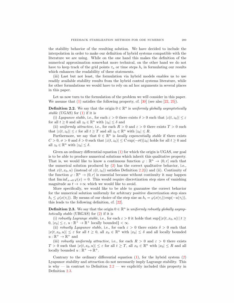
The limit cycle shrinks to the origin as Atol, Rtol → 0, but exists for all Atol,Rtol > 0. This is also visible from Figure 2, which shows the logarithm of thesquared Euclidean norm along the numerical solution for Atol = Rtol = 10−2 onthe left and for Atol = Rtol = 10−3 on the right. Obviously, the numerical solutionsare not asymptotically stable.
We will reconsider system (2.4) in Example 4.16, below, where we apply one ofthe methods proposed in this paper.
292 IASSON KARAFYLLIS AND LARS GRUNE
-4
-3,5
-3
-2,5
-2
-1,5
-1
-0,5
00 2000 4000 6000 8000 10000t
ln(V
(t))
-9
-8
-7
-6
-5
-4
-3
-2
-1
00 2000 4000 6000 8000t
ln(V
(t))
Figure 2. Logarithm of the squared Euclidean norm V (t) =
|x(t)|2 of the numerical solution for Example 2.4 with Atol =Rtol = 10−2 (left) and Atol = Rtol = 10−3 (right)
3. Small-gain methodology. One of the tools used in mathematical control the-ory for nonlinear feedback design is the methodology based on small-gain results.The method was first used in [20] where a nonlinear small-gain result based on thenotion of input-to-state stability (ISS, see [32]) was presented. Since then it hasbeen applied successfully to many feedback stabilization problems. Recently, thesmall-gain theorem was extended to general control systems including hybrid sys-tems (see [23]) and is thus applicable for the solution of problem (P2) for certainclasses of nonlinear systems (1). Here we apply the method to two types of sys-tems. The first is a system in triangular form which is called cascade in the controlliterature. In Section 5, below, we will see that this particular structure is suitablefor handling discretizations of certain PDEs.
We consider the system
z = f0(z) (13)
x1 = −a1(x1)x1 + f1(z)
xi = −ai(xi)xi + fi(z, x1, . . . , xi−1), i = 2, . . . , n (14)
with z ∈ Rm and x = (x1, . . . , xn)′ ∈ Rn. Here f0 : Rm → Rm, f1 : Rm → R,fi : Rm × Ri−1 → R and ai : R → R, i = 2, . . . , n are locally Lipschitz mappingswith f0(0) = 0, f1(0) = . . . = fn(0, 0, . . . , 0) = 0. We assume that there existconstants Li > 0, i = 1, . . . , n such that
ai(y) ≥ Li for all y ∈ R (15)
We also assume that 0 ∈ Rm is UGAS for (13). Under these assumptions, usingthe fact that system (13), (14) has a cascade structure, we may prove by inductionover n that the system is UGAS.
The proof for n = 1 is based on the fact that for every x10 ∈ R and for everymeasurable u : R+ → R the solution of x1 = −a1(x1)x1 + u with initial conditionx1(0) = x10 satisfies
FEEDBACK STABILIZATION METHODS FOR ODE NUMERICS 293
|x1(t)| ≤ exp
(−L1
2t
)|x10|+
1
L1sup
0≤s≤t|u(s)| for all t ≥ 0 (16)
Consequently, we obtain |x1(t)| ≤ exp(−L1
2 t)|x10|+ 1
L1sup0≤s≤t |f1(z(s))| for the
the solution of x1 = −a1(x1)x1 + f1(z), i.e., it is uniformly ISS with respect to theinput z ∈ Rm. Since 0 ∈ Rm is UGAS for (13), a well-known corollary of the small-gain theorem for systems in cascade guarantees UGAS for the composite system.For n ≥ 2 this argument is used inductively.
Now suppose that a stable numerical scheme is available for (13), i.e., there existfunctions ϕ ∈ C0(Rm; (0, r]), r > 0 and F0 :
⋃z∈Rm ([0, ϕ(z)]× z) → Rm with
F0(h, 0) = 0 for all h ∈ [0, ϕ(0)] and limh→0+ F0(h, z) = f0(z), for all z ∈ Rm suchthat 0 ∈ Rm is URGAS for the hybrid system (2) with F = F0. Then we proposethe following first order numerical scheme for the subsystem (14).
x1(t+ h) = x1(t)− ha1(x1(t))x1(t+ h) + hf1(z(t))
xi(t+ h) = xi(t)− hai(xi(t))xi(t+ h) + hfi(z(t), x1(t), . . . , xi−1(t)),
i = 2, . . . , n
(17)
The above scheme is a partitioned scheme which treats the state xi and the statesz, x1, . . . , xi−1 in different ways. The continuous dynamics of the resulting hybridsystem are
z(t) = F0(hi, z(τi))
x1(t) =−a1 (x1(τi))
1 + hia1 (x1(τi))x1(τi) +
1
1 + hia1 (x1(τi))f1(z(τi)) (18)
xj(t) =−aj (xj(τi))
1 + hiaj (xj(τi))xj(τi) +
1
1 + hiaj (xj(τi))fj(z(τi), x1(τi), . . . , xj−1(τi))
for j = 2, . . . , n. For this scheme the following theorem holds.
Theorem 3.1. The origin 0 ∈ Rm × Rn is URGAS for system (18).
The proof of this theorem, which can be found at the end of this section, relies onthe following technical lemma which is based on the variations of constants formula.
Lemma 3.2. Let a : R→ R be a continuous function with L = infy∈R a(y) > 0 andr > 0 be a constant. Then for every sequence hi∞0 with hi ∈ (0, r] for all i ≥ 0,for every locally bounded function v : R+ → R and for every x0 ∈ R the solution of
x(t) =−a (x(τi))
1 + hia (x(τi))x(τi) +
1
1 + hia (x(τi))v(τi), t ∈ [τi, τi+1)
τi+1 = τi + hi , hi ∈ (0, r] , x(t) ∈ R(19)
with initial condition x(0) = x0 ∈ R, τ0 = 0 satisfies
|x(t)| ≤ exp (σ r) |x0| exp (−σ t) +1
σ Lsup
0≤s≤t|v(s)| for all t ∈ [0, sup
i≥0τi) (20)
where σ > 0 is any constant such that 11+s ≤ exp(−σ s) for all s ∈ [0, rL], i.e.,
σ ≤ ln(1+rL)rL .

294 IASSON KARAFYLLIS AND LARS GRUNE
Proof. For every i ≥ 0 the variations of constants formula implies
x(τi+1) = x0
i∏j=0
(1 + hja (x(τj)))−1 +
i∑j=0
hjv(τj)
i∏k=j
(1 + hka (x(τk)))−1
(21)
Using the definition of L, we obtain the following bound from (21)
|x(τi+1)| ≤ |x0|i∏
j=0
(1 + hjL)−1 + maxj=0,...,i
|v(τj)|i∑
j=0
hj i∏k=j
(1 + hkL)−1
(22)
Now the definition of σ implies
i∑j=0
hj i∏k=j
(1 + hkL)−1
≤i∑
j=0
hj i∏k=j
exp(−σ Lhk)
=
i∑j=0
[hj exp(−σ L(τi+1 − τj))] = exp(−σ Lτi+1)
i∑j=0
[exp(σ Lτj)
∫ τj+1
τj
ds
]
≤ exp(−σ Lτi+1)
i∑j=0
[∫ τj+1
τj
exp(σ Ls)ds
]
= exp(−σ Lτi+1)
∫ τi+1
0
exp(σ Ls)ds ≤ 1
σ L
which in conjunction with (22) implies
|x(τi+1)| ≤ |x0| exp (−σ τi+1) +1
σ Lmax0≤j≤i
|v(τj)| (23)
for all i ≥ 0. Now for every i ≥ 0 and t ∈ [τi, τi+1) it holds that
|x(t)| ≤ max|x(τi)|, |x(τi+1)|. (24)
Combining (23) and (24) finishes the proof.
Proof of Theorem 3.1. We proceed by induction over n. For n = 0, the asser-tion follows immediately from the assumption on F0. For n → n + 1, Lemma 3.2guarantees
|xn+1(t)| ≤ exp (σ r) |xn+1(0)| exp (−σ t) +1
σ Ln+1sup
0≤s≤t|fn+1(z(s), . . . , xn(s))| ,
where σ > 0 is a constant with 11+s ≤ exp(−σ s) for all s ∈ [0, rmaxi=1,...,n+1(Li)].
Now Remark 3.2(b) in [23] (for systems in cascade) guarantees URGAS.
In Theorem 3.1 we use the special triangular cascade structure of (18). Indeed,due to this cascade structure we could also have derived the result from the dis-crete time Gronwall lemma. The following application shows that with small-gainarguments we can also handle more complex coupling structures. Consider theequation
xi = −ai(xi)xi + fi(x−i), i = 1, . . . , n (25)
with x = (x1, . . . , xn)T ∈ Rn and x−i = (x1, . . . , xi−1, xi+1, . . . , xn)T ∈ Rn−1. Herefi : Rn−1 → R and ai : R→ R are supposed to be locally Lipschitz for i = 1, . . . , n.
FEEDBACK STABILIZATION METHODS FOR ODE NUMERICS 295
We assume the existence of constants Li > 0 and Gij > 0, i, j = 1, . . . , n, with
ai(xi) ≥ Li and |fi(x−i)| ≤ maxj 6=i
Gij |xj | for all x ∈ Rn. (26)
Systems of the form (25) under the assumption (26) are frequently found in theneural networks literature, in particular for Hopfield neural networks, see [31] andthe references therein.
Again we consider a partitioned first order numerical scheme which is here of theform
xi(t+ h) = xi(t)− hai(xi(t))xi(t+ h) + hfi(x−i(t)), i = 1, . . . , n. (27)
The resulting hybrid system can be written in explicit form as
xj(t) =−aj(xj(τi))
1 + hiaj(xj(τi))xj(τi) +
1
1 + hiaj(xj(τi))fj(x−j(τi)), j = 1, . . . , n (28)
with τi and hi as in (2) where we use the constant step size selection ϕ ≡ r > 0.by virtue of Lemma 3.2 and recent small-gain results in [24] the following resultfollows. Observe that the resulting scheme is explicit and does not require aniterative solution of nonlinear equations for its implementation.
Theorem 3.3. The origin 0 ∈ Rn is URGAS for system (27) provided that foreach p = 2, . . . , n the inequality
Gi1i2Gi2i3 · · ·Gipi1 <(
ln(1 + rmaxL1, . . . , Ln)rmaxL1, . . . , Ln
)pLi1Li2 · · ·Lip (29)
holds for all ij ∈ 1, . . . , n with ij 6= ik for j 6= k.
Condition (29) is termed a cyclic or cycle small-gain condition in mathematicalsystems theory, cf. [3], [24] or [36]. For r → 0 we obtain
ln(1 + rmaxL1, . . . , Ln)rmaxL1, . . . , Ln
→ 1
and we recover the cyclic small-gain condition Gi1i2Gi2i3 · · ·Gipi1 < Li1Li2 · · ·Lipwhich guarantees that 0 ∈ Rn is UGAS for the continuous time system (25). Pro-vided that this inequality holds, (29) gives a condition on the upper bound on thetime step ϕ ≡ r such that the asymptotic stability carries over to the numericalapproximation.
Finally, note that Theorem 3.3 can easily be adapted to other classes of largescale systems which can be decomposed into smaller subsystems.
4. Lyapunov function based Step Selection. While the small-gain methodol-ogy is suitable for systems of differential equations with particular structures, itcannot be applied to general systems in a systematic way. On the other hand,Lyapunov-based feedback design methods can be applied to general nonlinear sys-tems of differential equations and yield explicit formulas for the feedback law (see[33]). In this section we apply the Lyapunov-based feedback design methodology forthe solution of Problems (P1) and (P2). It is well known that Lyapunov functionsexist for every asymptotically stable ODE and in many applications one can evengive explicit formulas for these functions (some examples can be found in Section6). However, even if a Lyapunov function is not exactly known, under suitable as-sumptions on the ODE, certain structural properties of the Lyapunov function canbe obtained (cf., e.g., Proposition 4.4, below) and used in our context. Hence, themain task of this section is to derive conditions under which the Lyapunov function
296 IASSON KARAFYLLIS AND LARS GRUNE
for the ODE system can be used in order to conclude stability for the hybrid system(2) and thus for the numerical approximation of system (1).
The results will be developed in the following way. First we provide some back-ground material needed for the derivation of the main results in Section 4.1. InSection 4.2 we consider general consistent Runge-Kutta schemes and provide suf-ficient conditions for the solvability of Problem (P1) and (P2). The results arespecialized for the explicit Euler method. Finally, in Section 4.3, we present specialresults for the implicit Euler scheme.
4.1. Background Material. The crucial technical result that allows the use ofLyapunov functions for hybrid systems of the form (2) is the following lemma.
Lemma 4.1. Consider system (2) and suppose that there exist a continuous, pos-itive definite and radially unbounded function V : Rn → R+ and a continuous,positive definite function W : Rn → R+ such that for every x ∈ Rn the followinginequality holds for all h ∈ [0, ϕ(x)].
V (x+ hF (h, x)) ≤ V (x)− hW (x) (30)
Then the origin 0 ∈ Rn is URGAS for system (2).
Proof. Notice first that by virtue of (3) there exist a function a ∈ K∞ such thatfor each x0 ∈ Rn and h ∈ [0, ϕ(x0)] the solution y(t) of y(t) = F (h, x0), y(0) = x0
exists for all t ∈ [0, h] and satisfies
|y(t)| ≤ a (|x0|) for all t ∈ [0, h]. (31)
This a can be chosen, e.g., as a(s) = s(1 + rM(s)) for M from (3).Now consider R ≥ 0 and the solution x(t, x0, u) of (2) with initial condition
x(0) = x0 satisfying |x0| ≤ R. Since V : Rn → R+ is continuous, positive definiteand radially unbounded, it follows from Lemma 3.5 in [25] that there exist functionsa1, a2 ∈ K∞ with
a1 (|x|) ≤ V (x) ≤ a2 (|x|) for all x ∈ Rn. (32)
Using induction over i and (30) we obtain
V (x(τi, x0, u)) ≤ V (x0) for all i ≥ 0. (33)
Inequality (33) in conjunction with (32) and (31) shows that
|x(t, x0, u)| ≤ a(a−1
1 (a2 (|x0|)))
for all t ∈ [0, sup τi). (34)
Moreover, inequality (33) implies that the sequence x(τi, x0, u) is bounded, whichcombined with the fact that u : R+ → R+ is locally bounded, implies that tmax =sup τi = +∞. Consequently, estimate (34) guarantees both robust Lagrange androbust Lyapunov stability, i.e., Definition 2.3(i) and (ii). In order to prove URGASit remains to show uniform robust global attractivity, i.e., Definition 2.3(iii). Tothis end, we next establish that for every ε > 0 the inequality
V (x(τi, x0, u)) ≤ a1(a−1(ε)) for all i ∈ Z+ with τi ≥a2 (R)
w(ε,R), (35)
holds with
w(ε,R) := minW (x) : a−1
2
(a1(a−1(ε))
)≤ |x| ≤ a
(a−1
1 (a2 (R)))
> 0. (36)
Using (32), (35) and (31) this property implies |x(t, x0, u)| ≤ ε for all t ≥ T = r +a2(R)w(ε,R) . Since T is independent of u, this shows Uniform Robust Global Attractivity.

FEEDBACK STABILIZATION METHODS FOR ODE NUMERICS 297
It remains to prove (35) which we do by contradiction. Let ε > 0 be arbitrary.
Suppose that (35) does not hold, i.e., that there exists i ≥ 0 with τi ≥ a2(R)w(ε,R)
such that V (x(τi)) > a1(a−1(ε)). By virtue of (30) it follows that V (x(τk, x0, u)) >a1(a−1(ε)), for all k = 0, . . . , i. The previous inequality in conjunction with inequal-ities (30), (34) and definition (36) implies V (x(τk+1, x0, u)) ≤ V (x(τk, x0, u)) −hkw(ε,R) for all k = 0, . . . , i − 1. Thus, we obtain V (x(τi, x0, u)) ≤ V (x0) −w(ε,R)
∑i−1k=0 hk. Notice that inequality (32) implies that V (x0) ≤ a2 (R). Since
τi =∑i−1k=0 hk, we obtain a1(a−1(ε)) < a2 (R) − τiw(ε,R) ≤ 0, a contradiction.
This finishes the proof.
The essential problem with the use of Lemma 4.1 is the knowledge of the Lya-punov function V . In the sequel, we will use a Lyapunov function for the continuous-time system (1) in order to construct a Lyapunov function for its hybrid numericalapproximation. To this end we use the following definition.
Definition 4.2. A positive definite, radially unbounded function V ∈ C1(Rn;R+)is called a Lyapunov function for system (1) if the inequality
∇V (x)f(x) < 0 (37)
holds for all x ∈ Rn\0.
In the following subsections, we show that under certain assumptions a Lyapunovfunction V for the original system (1) can be used as a control Lyapunov function(see [1, 4, 33, 34]) for its numerical approximation (2) in order to design the stepsize function ϕ : Rn → (0, r] in problems (P1) and (P2). For this purpose we needthe following technical results whose proofs are provided in the appendix.
Lemma 4.3. Let V ∈ C1(Rn;R+) be a Lyapunov function for system (1). Thenthe following statements hold.
(i) There exists a locally Lipschitz, positive definite function W : Rn → R+ suchthat the inequality
W (x) ≤ −∇V (x)f(x) (38)
holds for all x ∈ Rn.(ii) Let lf : Rn → (0,+∞) be a continuous function satisfying
lf (x) ≥ sup
|f(y)− f(z)||y − z|
: y, z ∈ Rn , y 6= z , maxV (z), V (y) ≤ V (x)
for all x ∈ (Rn\0). Then for every positive constant b > 0 there exists a
continuous, positive definite function W : Rn → R+ such that the inequality
V (z(h, x)) ≤ V (x)− hW (x) (39)
holds for all x ∈ Rn and h ∈ [0, ϕ(x)] with
ϕ(x) :=b
lf (x). (40)
(iii) Let b > 0, W : Rn → R+ be the function from statement (i), above, and letlbW : Rn → R+ be a continuous positive definite function satisfying
lbW (x) ≥ sup
|W (y)−W (z)||y − z|
: y, z ∈ Rn , y 6= z , max |y| , |z| ≤ exp(b) |x|

298 IASSON KARAFYLLIS AND LARS GRUNE
for all x ∈ Rn \ 0. If there exist constants ε, c > 0 such that
|x| lbW (x) ≤ cW (x) (41)
holds for all x ∈ Bε(0), then for each λ ∈ (0, 1) inequality (39) holds for all
x ∈ Rn and h ∈ [0, ϕ(x)] with W (x) := λW (x) where ϕ ∈ C0(Rn; (0,+∞)) isany function satisfying
ϕ(x) ≤ min
b
lf (x),
(1− λ) exp(−b)W (x)
|x| lbW (x)lf (x)
for all x ∈ Rn\0. (42)
Proposition 4.4. Suppose that f : Rn → Rn is a continuously differentiable vectorfield, 0 ∈ Rn is UGAS and locally exponentially stable for (1). Then there exist aLyapunov function V ∈ C1(Rn;R+) for (1), a symmetric, positive definite matrixP ∈ Rn×n and constants ε, µ > 0 such that the following inequalities hold.
V (x) = x′Px for all x ∈ Bε(0) (43)
∇V (x)f(x) ≤ −µ |x|2 for all x ∈ Rn (44)
4.2. General Runge-Kutta Schemes. In this section we will provide two the-orems giving different sufficient conditions for the solvability of the problems (P1)and (P2) for general Runge-Kutta schemes based on a Lyapunov function V forthe continuous dynamical system (1). Since the expressions involved in these theo-rems can be quite involved, in addition we present a simple computational methodbased on our approach in Algorithm 4.14. Our first result uses information on thederivatives of V as formulated in the following theorem.
Theorem 4.5. Suppose that there exists an integer p ≥ 1 and a Lyapunov functionV ∈ C(p+1)(Rn;R+) for system (1). Consider system (2) corresponding to a Runge-Kutta scheme for (1) and suppose that
(i) for each fixed x ∈ Rn the mapping [0, ϕ(x)] 3 h→ V (x+ hF (h, x)) is (p+ 1)times continuously differentiable
(ii) the Runge-Kutta scheme is consistent with order p ≥ 1, i.e., for every x ∈Rn and h ∈ [0, ϕ(x)] there exists constant K > 0 such that the inequality|z(h, x)− x− hF (h, x)| ≤ Khp+1 holds
(iii) there exists a constant λ ∈ (0, 1) such that for every x ∈ Rn the inequalityϕ(x) minj=1,...,pKj(x) ≤ (λ− 1)LfV (x) holds, where
Kj(x) := max j∑i=2
si−2
i!LifV (x)
+sj−1
(j + 1)!
∂j+1
∂ hj+1V (x+ hF (h, x)) : h, s ∈ [0, ϕ(x)]
for j ≥ 2 and K1(x) := 1
2 max
∂2
∂ h2V (x+ hF (h, x)) : h ∈ [0, ϕ(x)]
.
Then 0 ∈ Rn is URGAS for system (2).
Proof. Since for each fixed x ∈ Rn the mapping [0, ϕ(x)] 3 h → g(h) = V (x +hF (h, x)) is (p + 1) times continuously differentiable, by Taylor’s theorem for allj = 1, . . . , p and h ∈ [0, ϕ(x)] we have
V (x+ hF (h, x)) = g(h) ≤ g(0) +
j∑i=1
hi
i!
dig
dhi(0) +
hj+1
(j + 1)!max
0≤ξ≤h
dj+1g
dhj+1(ξ). (45)
FEEDBACK STABILIZATION METHODS FOR ODE NUMERICS 299
Since the Runge-Kutta scheme is of order p ≥ 1, we have
dig
dhi(0) = LifV (x) for all i = 1, . . . , p. (46)
Consequently, for all j = 1, . . . , p and h ∈ [0, ϕ(x)] we obtain
V (x+ hF (h, x)) ≤ V (x) + hLfV (x) + h2Kj(x) (47)
or, equivalently, for all h ∈ [0, ϕ(x)]
V (x+ hF (h, x)) ≤ V (x) + hLfV (x) + h2 minj=1,...,p
Kj(x) (48)
The inequality ϕ(x) minj=1,...,pKj(x) ≤ (λ − 1)LfV (x) in conjunction with (48)implies V (x + hF (h, x)) ≤ V (x) + λhLfV (x). Thus, Lemma 4.1 implies that0 ∈ Rn is URGAS for system (2).
Remark 4.6. (a) Theorem 4.5 implies the following property for a Runge-Kuttascheme with order p ≥ 1 satisfying (7) and a system of ODEs (1) with f ∈C(p+1)(Rn;Rn) for which 0 ∈ Rn is UGAS:
If a Lyapunov function V ∈ C(p+1)(Rn;R+) for (1) is available for which thereexist constants K,Λ > 0, an integer q ≥ 1 and a neighborhood N ⊂ Rn with 0 ∈ Nsuch that ∇V (x)f(x) ≤ −K |x|q+1
and |f(x)| ≤ Λ |x|q for all x ∈ N , then for everyλ ∈ (0, 1) and every compact S ⊂ Rn we can find h > 0 sufficiently small such thatV (x+ hF (h, x)) ≤ V (x) + λh∇V (x)f(x) for all x ∈ S.
This fact follows from (7) and the observation that K1(x) = O(|x|q+1) for x closeto zero. Consequently, the numerical solution of (1) with sufficiently small step sizewill give the correct dynamic behavior.
(b) The functions Kj , j ≥ 1 involved in hypothesis (iii) of Theorem 4.5 are ingeneral difficult to be computed for higher order Runge-Kutta schemes. However,for the explicit Euler scheme F (h, x) = f(x) the function K1(x) can be computedwithout difficulty as K1(x) := 1
2 maxf ′(x)∇2V (x+ hf(x))f(x) : h ∈ [0, ϕ(x)]
.
Consequently, we obtain the following corollary.
Corollary 4.7. (Explicit Euler method) Suppose that there exists a Lyapunovfunction V ∈ C2(Rn;R+) for system (1) where f ∈ C0(Rn;Rn) is locally Lipschitzand that there exist constants r ≥ δ > 0, λ ∈ (0, 1) and a neighborhood N ⊂ Rnwith 0 ∈ N and
δ q(x) ≤ −2(1− λ)∇V (x)f(x) for all x ∈ N , (49)
where q(x) := maxf ′(x)∇2V (x+ hf(x))f(x) : h ∈ [0, r]
. Then Problem (P1)
is solvable for system (2) with F (h, x) := f(x) and Problem (P2) is solved for anyϕ ∈ C0(Rn; (0, r]) satisfying
ϕ(x)q(x) ≤ −2(1− λ)∇V (x)f(x) for all x ∈ Rn. (50)
Proof. Inequality (49) guarantees the existence of ϕ ∈ C0(Rn; (0, r]) satisfying (50),e.g., we may define ϕ(x) := δ if x ∈ N , ϕ(x) := δ if x /∈ N and q(x) ≤ 0, and
ϕ(x) := min− 2(1−λ)∇V (x)f(x)
q(x) , δ
else. The rest is a consequence of Theorem
4.5 and the fact that 2K1(x) ≤ q(x) for all x ∈ Rn.
300 IASSON KARAFYLLIS AND LARS GRUNE
Remark 4.8. Corollary 4.7 implies the following property for a system of ODEs(1) with f ∈ C0(Rn;Rn) being locally Lipschitz for which 0 ∈ Rn is UGAS:
If a Lyapunov function V ∈ C2(Rn;R+) for (1) is available for which there existconstants K,Λ > 0, an integer q ≥ 1 and a neighborhood N ⊂ Rn with 0 ∈ Nsuch that ∇V (x)f(x) ≤ −K |x|2q and |f(x)| ≤ Λ |x|q for all x ∈ N , then for everyλ ∈ (0, 1) and every compact S ⊂ Rn we can find h > 0 sufficiently small such thatV (x+ hf(x)) ≤ V (x) + λh∇V (x)f(x) for all x ∈ S.
This fact follows from (7) and the observation that q(x) = O(|x|2q) for x closeto zero. Note the difference to Remark 4.6(a): due to the particular structure of
the Euler method here we only need to require ∇V (x)f(x) ≤ −K |x|2q instead of
∇V (x)f(x) ≤ −K |x|q+1.
The following second theorem for general Runge-Kutta schemes provides alter-native sufficient conditions for the solvability of problem (P2) based on a Lyapunovfunction for the ODE (1). The conditions are different from those in Theorem 4.5,in particular they do not require the Lyapunov function to be smoother than C1.
Theorem 4.9. Consider system (2) corresponding to a Runge-Kutta scheme for(1) of order p ≥ 1 satisfying (7), (8), (9) for certain ϕ ∈ C0(Rn; (0,+∞)). Supposethat
(i) there exist a Lyapunov function V ∈ C1(Rn;R+) for system (1) and a con-
tinuous, positive definite function W : Rn → R+ such that (39) holds for allx ∈ Rn and h ∈ [0, ϕ(x)]
(ii) there exists b ≥ 0 with |z(h, x)| ≤ exp(b) |x| and |x+ hF (h, x)| ≤ exp(b) |x|for all x ∈ Rn and h ∈ [0, ϕ(x)]
(iii) there exists a constant λ ∈ (0, 1) such that
ϕ(x) ≤
((1− λ) W (x)
lbV (x)C(x)
) 1p
for all x ∈ Rn \ 0, (51)
where lbV (x) := max |∇V (z)| : z ∈ Rn , |z| ≤ exp(b) |x| for all x ∈ Rn andC : Rn → R+ is a continuous positive definite function satisfying the inequality|z(h, x)− x− hF (h, x)| ≤ C(x)hp+1 for all x ∈ Rn and h ∈ [0, ϕ(x)].
Then 0 ∈ Rn is URGAS for system (2).
Proof. Utilizing hypotheses (i) and (ii) and
lbV (x) ≥ sup
|V (z)− V (y)||z − y|
: z, y ∈ Rn , max |y| , |z| ≤ exp(b) |x| , z 6= y
,
for all x ∈ Rn \ 0 and h ∈ [0, ϕ(x)] we obtain
V (x+ hF (h, x)) ≤ |V (x+ hF (h, x))− V (z(h, x))|+ V (z(h, x))
≤ lbV (x) |x+ hF (h, x)− z(h, x)|+ V (x)− hW (x)
For all x ∈ Rn and h ∈ [0, ϕ(x)] this inequality in conjunction with (9) gives
V (x+ hF (h, x)) ≤ V (x)− h(W (x)− hplbV (x)C(x)
),
where C : Rn → R+ is the continuous positive definite function from (iii). Togetherwith (51) this implies
V (x+hF (h, x)) ≤ V (x)−λhW (x) for all x ∈ Rn\0 and all h ∈ [0, ϕ(x)]. (52)

FEEDBACK STABILIZATION METHODS FOR ODE NUMERICS 301
Observing that (3) guarantees that (52) holds for x = 0 as well, Lemma 4.1 impliesthat 0 ∈ Rn is URGAS for system (2).
Remark 4.10. The proof of Lemma 4.3 (see formula (87) in the appendix), in-equality (10) and Theorem 4.8 imply the following fact for a Runge-Kutta schemewith order p ≥ 1 and a system of ODEs (1) with f ∈ Cp(Rn;Rn) for which 0 ∈ Rnis UGAS:
If a Lyapunov function V ∈ C2(Rn;R+) for (1) is available for which there existconstants K,Λ, c > 0, an integer q ≥ 1 and a neighborhood N ⊂ Rn with 0 ∈ N suchthat ∇V (x)f(x) ≤ −K |x|q+1
, |f(x)| ≤ Λ |x|q and (41) with W (x) := −∇V (x)f(x)holds for all x ∈ N, then for every λ ∈ (0, 1) and every compact S ⊂ Rn we can findh > 0 sufficiently small such that V (x + hF (h, x)) ≤ V (x) + λh∇V (x)f(x) for allx ∈ S. This property follows from (10) and the observation that
lbV (x) := max |∇V (z)| : z ∈ Rn , |z| ≤ exp(b) |x| = O (|x|)
for x close to zero. The reader should notice that in contrast to Remark 4.6(a) weneed less smoothness of V here.
The following example illustrates Remarks 4.6 and 4.10.
Example 4.11. Consider the three planar systems with x = fk(x), k = 1, 2, 3,x = (x1, x2)′ ∈ R2 with
f1(x) :=
[−x1 + x2
−x1 − x2
], f2(x) :=
[− |x|2 x1 + x2
−x1 − |x|2 x2
], f3(x) := |x|2
[−x1 + x2
−x1 − x2
].
For each of the systems we can use the Lyapunov function V (x) = |x|2. We obtain
∇V (x)f1(x) = −2 |x|2 , ∇V (x)f2(x) = −2 |x|4 , ∇V (x)f3(x) = −2 |x|4 .
Clearly, for k = 1, 2, 3 there exist constants Λk > 0, integers qk ≥ 1 and a neigh-borhood N ⊂ R2 with 0 ∈ N such that |fk(x)| ≤ Λk |x|qk for all x ∈ N withq1 = q2 = 1 and q3 = 3. Remark 4.6(a) shows that for k = 1 and k = 3 we canapply any consistent Runge-Kutta numerical scheme with sufficiently small stepsize and produce a qualitatively correct numerical solution. The same conclusionis derived from Remark 4.10 (notice that (41) holds for each of the systems with
Wk(x) := −∇V (x)fk(x), lbW1(x) = 4 exp(b) |x|, lbW2
(x) = lbW3(x) = 8 exp(3b) |x|3
for a neighborhood N ⊂ R2 with 0 ∈ N ). This is confirmed by the numericalsimulations for the Euler and Heun scheme shown in Figure 3 for constant step sizeh = 0.2.
On the other hand, the requirements presented in Remark 4.6(a) or Remark 4.10are not fulfilled for k = 2. Similarly, the requirements presented in Remark 4.8 arenot fulfilled for k = 2. Consequently, we cannot conclude that the application ofany consistent Runge-Kutta numerical scheme with sufficiently small step size willproduce a qualitatively correct numerical solution. Numerical solutions with theexplicit Euler and the Heun scheme confirm these results, cf. Figure 4. For the sys-tem x = f2(x) both schemes applied with constant h > 0 exhibit an asymptoticallystable limit cycle, which shrinks to the origin as h→ 0, but exists for all h > 0.
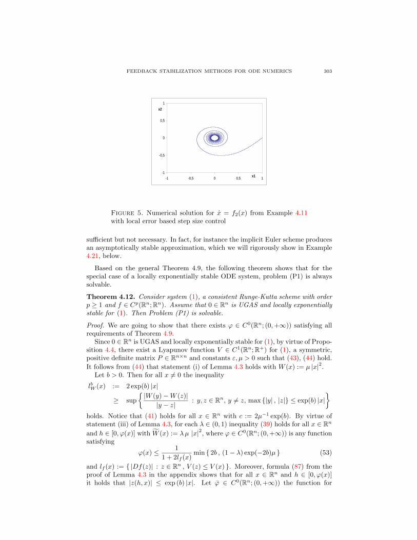
Observe that a local error based step size control does not resolve the lack ofasymptotic stability of the origin for our second example. Figure 5 shows thesolutions for this method using the Euler and Heun schemes outlined in Example2.4 for parameters P = 1, Rtol = 0 and Atol = 10−4. Again, the numerical solution

302 IASSON KARAFYLLIS AND LARS GRUNE
-1
-0,5
0
0,5
1
-1 -0,5 0 0,5 1x1
x2
EULERHEUN
-1
-0,5
0
0,5
1
-1 -0,5 0 0,5 1x1
x2
EULERHEUN
Figure 3. Numerical solution for x = f1(x) (left) and x = f3(x)(right) from Example 4.11 with initial condition x = (1, 0) usingthe explicit Euler and the Heun method
-1
-0,5
0
0,5
1
-1 -0,5 0 0,5 1x1
x2
-1
-0,5
0
0,5
1
-1 -0,5 0 0,5 1x1
x2
Figure 4. Numerical solution for x = f2(x) from Example 4.11with initial condition x = (1, 0) using the explicit Euler (left) andthe Heun method (right)
exhibits an asymptotically stable limit cycle which shrinks to the origin as Atol→ 0,but exists for all Atol > 0.
This behavior is expected from our theoretical results, since the fact that therequirements of Remarks 4.6(a), 4.8 and 4.10 are not satisfied indicates that forthis system and the chosen explicit methods any step size control method will failto provide an asymptotically stable solution.
We would like to emphasize that Theorem 4.5 and Theorem 4.9 and the respectiveRemarks 4.6(a), 4.8 and 4.10 derived from these theorems do not state that theredoes not exist a Runge-Kutta scheme which produces an asymptotically stableapproximation for system x = f2(x), since the conditions in these results are merely
FEEDBACK STABILIZATION METHODS FOR ODE NUMERICS 303
-1
-0,5
0
0,5
1
-1 -0,5 0 0,5 1x1
x2
Figure 5. Numerical solution for x = f2(x) from Example 4.11with local error based step size control
sufficient but not necessary. In fact, for instance the implicit Euler scheme producesan asymptotically stable approximation, which we will rigorously show in Example4.21, below.
Based on the general Theorem 4.9, the following theorem shows that for thespecial case of a locally exponentially stable ODE system, problem (P1) is alwayssolvable.
Theorem 4.12. Consider system (1), a consistent Runge-Kutta scheme with orderp ≥ 1 and f ∈ Cp(Rn;Rn). Assume that 0 ∈ Rn is UGAS and locally exponentiallystable for (1). Then Problem (P1) is solvable.
Proof. We are going to show that there exists ϕ ∈ C0(Rn; (0,+∞)) satisfying allrequirements of Theorem 4.9.
Since 0 ∈ Rn is UGAS and locally exponentially stable for (1), by virtue of Propo-sition 4.4, there exist a Lyapunov function V ∈ C1(Rn;R+) for (1), a symmetric,positive definite matrix P ∈ Rn×n and constants ε, µ > 0 such that (43), (44) hold.
It follows from (44) that statement (i) of Lemma 4.3 holds with W (x) := µ |x|2.Let b > 0. Then for all x 6= 0 the inequality
lbW (x) := 2 exp(b) |x|
≥ sup
|W (y)−W (z)||y − z|
: y, z ∈ Rn, y 6= z, max |y| , |z| ≤ exp(b) |x|
holds. Notice that (41) holds for all x ∈ Rn with c := 2µ−1 exp(b). By virtue ofstatement (iii) of Lemma 4.3, for each λ ∈ (0, 1) inequality (39) holds for all x ∈ Rn
and h ∈ [0, ϕ(x)] with W (x) := λµ |x|2, where ϕ ∈ C0(Rn; (0,+∞)) is any functionsatisfying
ϕ(x) ≤ 1
1 + 2lf (x)min 2b , (1− λ) exp(−2b)µ (53)
and lf (x) := |Df(z)| : z ∈ Rn , V (z) ≤ V (x) . Moreover, formula (87) from theproof of Lemma 4.3 in the appendix shows that for all x ∈ Rn and h ∈ [0, ϕ(x)]it holds that |z(h, x)| ≤ exp (b) |x|. Let ϕ ∈ C0(Rn; (0,+∞)) the function for
304 IASSON KARAFYLLIS AND LARS GRUNE
which (7), (8), (9) hold for all x ∈ Rn and h ∈ [0, ϕ(x)]. We notice that theinequality |x+ hF (h, x)| ≤ exp(b) |x| holds for all x ∈ Rn and h ∈ [0, ϕ(x)], whereϕ ∈ C0(Rn; (0,+∞)) is any function satisfying
ϕ(x) ≤ min
ϕ(x) ,
exp(b)
1 + ϕ(x)M (|x|)
for all x ∈ Rn (54)
and M : R+ → R+ is the continuous, non-decreasing function involved in (3).Next we show the existence of ϕ ∈ C0(Rn; (0,+∞)) satisfying (51). It suffices to
show that there exist constants δ > 0, λ ∈ (0, 1) and a neighborhood N ⊂ Rn with0 ∈ N such that
δp lbV (x)C(x) ≤ (1− λ)µλ |x|2 for all x ∈ N , (55)
where C : Rn → R+ is a continuous positive definite function satisfying the in-equality |z(h, x)− x− hF (h, x)| ≤ C(x)hp+1 for all x ∈ Rn and h ∈ [0, ϕ(x)]. LetN = Bρ(0), where ρ := ε exp(−b) and ε > 0 is the constant involved in (43).Clearly, (43) implies
lbV (x) ≤ 2 |P | exp(b) |x| for all x ∈ N , (56)
where P ∈ Rn×n is the symmetric, positive definite matrix involved in (43). Noticethat without loss of generality we may assume that there exists constant K > 0such that (10) holds with q = 1 for all x ∈ N and h ∈ [0, ϕ(x)] (the existence ofQ > 0 with |z(h, x)| ≤ Q |x| for all x ∈ N and h ≥ 0 is a consequence of localexponential stability). Consequently, by virtue of (10), (56), we can guarantee that
(55) holds for every λ ∈ (0, 1) with δ :=(
(1−λ)µλ2K|P | exp(b)
) 1p
. Therefore, from all the
above we conclude that we may define
ϕ(x) :=
min
δ , ϕ(x) , exp(b)
1+ϕ(x)M(|x|) ,κ
1+2lf (x)
, x ∈ N
min
δ , ϕ(x) , exp(b)
1+ϕ(x)M(|x|) ,κ
1+2lf (x) ,(
(1−λ)λµ|x|2lbV (x)C(x)
) 1p
, x /∈ N ,
where κ := min 2b , (1− λ) exp(−2b)µ , so that all requirements of Theorem 4.9are fulfilled. The proof is complete.
Remark 4.13. Theorem 4.12 is an existence result which does not give an explicitestimate for ϕ(x), i.e., it answers (P1) but does not solve (P2). However, similar toRemark 4.8 and 4.10 we can conclude that the numerical approximation is asymp-totically stable on each compact set S for sufficiently small step size h. Note thatlocal exponential stability is not a necessary condition for asymptotic stability ofexplicit Runge-Kutta schemes, as Example 4.11 shows: there 0 ∈ R2 is UGAS butnot locally exponentially stable for x = f3(x).
The calculations needed in order to verify whether a map ϕ meets the assump-tions of Theorem 4.5 or Theorem 4.9 are rather complex. However, given that theassumptions of one of these theorems are satisfied, an appropriate time step can beobtained by the following straightforward algorithm. Here we assume that we aregiven a Runge-Kutta scheme and a parameter λ ∈ (0, 1).
Algorithm 4.14. In each step of the computation:
(1) Set h := 2h (where h > 0 on the right hand side is the time step from theprevious step)

FEEDBACK STABILIZATION METHODS FOR ODE NUMERICS 305
(2) If V (x+ hF (h, x)) ≤ V (x) + λhLfV (x) then the time step h > 0 is accepted;otherwise set h := h/2 and go to (2)
Here V ∈ C2(Rn;R+) is a Lyapunov function for (1) for which there exist aconstant K > 0 and a neighborhood N ⊂ Rn with 0 ∈ N such that ∇V (x)f(x) ≤−K |x|2 for all x ∈ N . Using this algorithm, we do not have to compute the step sizefunction ϕ(x) that guarantees robust global asymptotic stability of the numericalapproximation. The following example illustrates this point.
Example 4.15. We consider four different explicit numerical schemes: the explicitEuler scheme, Heun’s scheme, the 2nd order improved polygonal scheme and Kutta’s3rd order scheme. The numerical schemes are applied to the planar system
x1 = −x1 + x22, x2 = −x2 − x1x2 (57)
using the Lyapunov function V (x) = (x21 +x2
2)/2. For all numerical schemes (exceptthe explicit Euler method) the calculation of the maximum allowed time step byusing Theorem 4.5 or Theorem 4.9 is very complicated. However, using Algorithm4.14, for each x we can determine the maximum h > 0 for which the inequalityV (x + hF (h, x)) ≤ V (x) + λhLfV (x) with λ = 1
2 holds. Figure 6 shows thegraph of the maximum allowable time step for the four numerical methods withx = (x1, 1)′ ∈ R2 and varying x1 ∈ R.
0
0,2
0,4
0,6
0,8
1
-15 -10 -5 0 5 10 15 20x1
h
HEUN
EULER
POLYGONAL
KUTTA
Figure 6. Maximum allowable time step determined by Algo-rithm 4.14 with λ = 1/2 for various numerical schemes and (57)with x = (x1, 1)′ ∈ R2
It should be noticed that for x1 close to zero all higher order schemes allow greatertime steps than the the explicit Euler method (notice that for x = (x1, 1)′ ∈ R2 andλ = 1
2 the maximum allowable time step for which the inequality V (x+hF (h, x)) ≤V (x) + λhLfV (x) holds for the explicit Euler method is h = 1
2 ). However, forlarge values of |x1| the maximum allowable time step for higher order schemes

306 IASSON KARAFYLLIS AND LARS GRUNE
are considerably smaller than the time step allowed by the explicit Euler method.This shows that a higher order method does not necessarily allow higher valuesfor the maximum allowable time step for which the inequality V (x + hF (h, x)) ≤V (x) + λhLfV (x) holds.
Example 4.16. We apply Algorithm 4.14 to the planar system (11). Figure 7shows the logarithm of the value of the Lyapunov function V (x) = x2
1 + x22 for the
numerical solution obtained by Heun’s 2nd order scheme with λ = 0.5 or λ = 0.9and initial condition (x1, x2) = (1, 0): the numerical solution exhibits convergenceto the globally exponentially stable equilibrium point 0 ∈ R2. In both cases thestep is selected once and remains constant thereafter (h = 0.277 for λ = 0.5 andh = 0.165 for λ = 0.9). Observe that in contrast to Example 2.4 here asymptoticstability of the numerical approximation is achieved.
-50
-45
-40
-35
-30
-25
-20
-15
-10
-5
00 2000 4000 6000 8000 10000t
ln(V
(t))
lambda=0.5lambda=0.9
Figure 7. Logarithm of the Lyapunov function V (x) = x21 + x2
2
along the numerical solution of (11) using Algorithm 4.14 withλ = 0.5 or λ = 0.9.
Since V (t) = −0.01V (t) for system (11), it is clear that the logarithm of theLyapunov function V (x) = x2
1 + x22 along the exact solution will be a straight line
with slope −0.01. As λ→ 1 our numerical result approaches this line at the cost ofusing smaller step sizes.
4.3. Implicit Runge-Kutta schemes. In this section we show how Lyapunovfunction based arguments can be used for implicit schemes. In order to keep thepresentation technically simple, we restrict ourselves to the implicit Euler schemefor which we can prove the following result.
Theorem 4.17. (Implicit Euler method) Suppose that there exists a convexLyapunov function for (1), where f ∈ C0(Rn;Rn) is locally Lipschitz. Let ϕ ∈C0(Rn; (0,+∞)) be such that the equation Y = x + hf(Y ) has a unique solution
FEEDBACK STABILIZATION METHODS FOR ODE NUMERICS 307
Y ∈ Rn for all h ∈ [0, ϕ(x)] and x ∈ Rn. Then for each r > 0 the origin 0 ∈Rn is URGAS for the corresponding system (2) with F (h, x) := f(Y ), ϕ(x) :=min ϕ(x) , r , where Y = x+ hf(Y ).
Proof. Define the functions
W1(x) := min −∇V (y)f(y) : y ∈ Rn , V (x) ≥ V (y) ≥ V (x)/2 W2(x) := 1
2rV (x).(58)
By virtue of (37) both functions are continuous and positive definite. Since V ∈C1(Rn;R+) is convex the following inequality holds for all x1, x2 ∈ Rn:
V (x1) +∇V (x1)x2 ≤ V (x1 + x2) (59)
Applying (59) with x1 = Y and x2 = −hf(Y ), where Y = x + hf(Y ) and h ∈[0, ϕ(x)], we get
V (x) = V (Y − hf(Y )) ≥ V (Y )− h∇V (Y )f(Y ) (60)
By virtue of (37), (60) implies that V (Y ) ≤ V (x). Now we distinguish the followingcases.
Case 1: V (Y ) ≥ 12V (x). In this case from (60) in conjunction with definition
(58) of W1 we obtainV (Y ) + hW1(x) ≤ V (x). (61)
Case 2: V (Y ) < 12V (x). In this case definition (58) of W2 implies
V (Y ) + hW2(x) ≤ V (x) (62)
for all h ∈ [0, r].Consequently, in both cases we obtain
V (Y ) ≤ V (x)− hW (x) (63)
for all h ∈ [0, ϕ(x)] and all x ∈ Rn, with Y = x + hf(Y ) and the positive definitefunction W (x) := min W1(x),W2(x). Thus, Lemma 4.1 yields the assertion.
The following corollary shows that Theorem 4.17 can be seen as a nonlineargeneralization of the well-known A-stability property of the implicit Euler method.
Corollary 4.18. Consider the system of ODEs x = Ax, x ∈ Rn where A ∈ Rn×n isa matrix whose eigenvalues have negativereal parts. Then the implicit Euler methodis URGAS for arbitrary step size h > 0.
Proof. As pointed out before (6), the implicit Euler method is well defined for eachstep size h > 0. Furthermore, the system x = Ax, x ∈ Rn admits the quadraticLyapunov function V (x) = x′Px, where P ∈ Rn×n is a symmetric, positive definitematrix, see [34, Theorem 5.7.18]. This Lyapunov function is obviously convex andthus Theorem 4.17 yields the assertion.
Remark 4.19. The main result in [13] guarantees that if n 6= 4, 5 then there existsa homeomorphism Φ : Rn → Rn with Φ(0) = 0, being a diffeomorphism on Rn \0and C1 on Rn such that the transformed system (1) y = DΦ(Φ−1(y))f
(Φ−1(y)
)admits the convex Lyapunov function V (y) := 1
2 |y|2. Consequently, the implicit
Euler can be applied to the transformed system, see [22]. However, for numericalpurposes the method is not practical, since the homeomorphism Φ : Rn → Rn isusually not available. On the other hand, for certain classes of systems Theorem4.17 is directly applicable. One such class are the so called gradient systems, asshown in the following example.
308 IASSON KARAFYLLIS AND LARS GRUNE
Example 4.20. Consider the following class of systems
x = f(x) = −(P (x) +G(x))(∇V (x))′, x ∈ Rn, (64)
where V ∈ C2(Rn;R+) is a positive definite, radially unbounded function withpositive definite Hessian and ∇V (0) = 0, P (x) ∈ Rn×n is a symmetric positivedefinite matrix with locally Lipschitz elements and G(x) ∈ Rn×n is a matrix withlocally Lipschitz elements with G′(x) = −G(x) for all x ∈ Rn. The class of systemsof the form (64) is a generalization of the class of the so-called gradient systems,see [35].
Under our assumptions, V is a convex Lyapunov function for (64). Hence,it follows from Theorem 4.17 that the implicit Euler scheme produces asymp-totically stable numerical solutions of of (64) for every r > 0, λ ∈ (0, 1) with
ϕ(x) := min
λLλ(x)+γ(x) , r
, where γ : Rn → R+ is a continuous function with
|f(x)| ≤ |x| γ (x) for all x ∈ Rn, Lλ : Rn → (0,+∞) is a continuous function
with Lλ(x) ≥ sup|f(z)−f(y)||z−y| : z, y ∈ Nλ(x) , z 6= y
for all x ∈ Rn \ 0 and
Nλ(x) := y ∈ Rn : |y − x| ≤ λ |x| .
We end this section by noting that Theorem 4.17 also applies to all systemsconsidered in Example 4.11.
Example 4.21. Consider again systems x = fk(x), k = 1, 2, 3 from Example 4.11.
Since these systems admit the convex Lyapunov function V (x) = |x|2, it followsfrom Theorem 4.17 that the implicit Euler scheme produces asymptotically stablesolutions for all systems x = fk(x), k = 1, 2, 3 of Example 4.11.
5. Application of the small-gain step selection. In this section we show anapplication of the small-gain based step selection method developed in Section 3 toa discretization of a PDE. Consider the infinite-dimensional dynamical system
∂ x
∂ t(t, z) + c
∂ x
∂ z(t, z) = b(x(t, z))x(t, z), z ∈ (0, 1], x(t, 0) = 0 (65)
with x(t, z) ∈ R, b : R → R being locally Lipschitz, c > 0 and initial conditionx(0, z) = x0(z), where x0 ∈ C1([0, 1];R) with x0(0) = dx0
dz (0) = 0, under thefollowing hypothesis
(H) There exists constant K ≥ 0 such that b(x) ≤ K for all x ∈ R.Using the method of characteristics and hypothesis (H), it can be shown that the
PDE (65) admits a unique classical solution x(t, · ) ∈ C1([0, 1];R) with x(t, 0) =∂ x∂ z (t, 0) = 0 for all t ≥ 0. Moreover, the zero solution is globally asymptotically
stable, since for every x0 ∈ C1([0, 1];R) with x0(0) = dx0
dz (0) = 0, the unique
classical solution x(t, · ) ∈ C1([0, 1];R) of (65) with initial condition x(0, z) = x0(z)satisfies x(t, z) = 0 for all t ≥ c−1z.
Using a uniform space grid of n+1 points with space discretization step ∆z = 1n ,
setting xi(t) = x(t, i∆z), i = 0, 1, . . . , n and approximating the spatial derivativeby the backward difference scheme
∂ x
∂ z(t, i∆z) ≈ x(t, i∆z)− x(t, (i− 1)∆z)
∆z=xi(t)− xi−1(t)
∆z
for i = 1, . . . , n, we obtain the following set of ordinary differential equations.
FEEDBACK STABILIZATION METHODS FOR ODE NUMERICS 309
x1 = −( c
∆z− b(x1)
)x1
xi = −( c
∆z− b(xi)
)xi +
c
∆zxi−1, i = 2, . . . , n
(66)
It is clear that system (66) has the structure of system (13), (14) with ai(xi) =c
∆z − b(xi) for i = 1, . . . , n. Moreover, if the space discretization step is selected sothat
K∆z < c (67)
holds for K ≥ 0 from Hypothesis (H), then inequalities (15) hold as well withLi = c
∆z − K for i = 1, . . . , n. Theorem 3.1 allows us to conclude that for everyh > 0 the numerical scheme
x1(t+ h) =x1(t)
1 + h(c
∆z − b(x1(t)))
xi(t+ h) =xi(t) + ch
∆zxi−1(t)
1 + h(c
∆z − b(xi(t))) , i = 2, . . . , n
(68)
will give the correct qualitative behavior.The reader should notice that for the case b(x) ≡ 0 inequality (67) is automati-
cally satisfied (with K = 0) and the numerical scheme (68) reduces to the so-calledimplicit upwind scheme for the advection equation, which is unconditionally stable.
6. Applications of the Lyapunov-based step selection. In this section wepresent some applications for the Lyapunov-based step selection method providedin Section 4. It should be emphasized that this method can in principle be appliedto all dynamical systems for which a Lyapunov function is known with a globallyasymptotically stable and locally exponentially stable equilibrium, cf. Theorem 4.12.However, as the following applications show, there are certain classes of systems forwhich we can guarantee more properties or which deserve special attention.
6.1. Solution of Nonlinear Programming Problems. There are many nonlin-ear programming problems which can be solved by constructing a dynamical sys-tem with a globally asymptotically stable equilibrium point which coincides withthe minimizer of the nonlinear programming problem, see [9, 37, 38, 39]. A specialfeature for such methods is that a Lyapunov function is available, however, theposition of the equilibrium point is not known (this is what we seek). Consider thefollowing nonlinear programming problem
min f(x) , x ∈ Rns.t. Ax = b,
(P)
where f ∈ C3(Rn;R) is strictly convex and radially unbounded with positive definiteHessian and A ∈ Rm×n, b ∈ Rm with m < n satisfies det(AA′) 6= 0. Under thesehypotheses there is a global minimum x∗ ∈ Rn of problem (P). Moreover, thereexists a vector z∗ ∈ Rm such that (x∗, z∗) ∈ Rn+m is the unique solution of theequations
∇f(x) + z′A = 0Ax = b.
(69)
Problem (P) may be solved by means of differential equations if we further as-
sume that the function G(x) =∣∣∇f(x)
(I −A′(AA′)−1A
) ∣∣2 + |Ax− b|2 is radially

310 IASSON KARAFYLLIS AND LARS GRUNE
unbounded. Indeed, the system
x = −(∇2f(x) (∇f(x) + z′A)
′+A′(Ax− b)
)z = −A (∇f(x) + z′A)
′ (70)
has the unique equilibrium point (x∗, z∗) ∈ Rn+m, which is UGAS for (70). This
fact can be proved by using the Lyapunov function V (x, z) = 12 |∇f(x) + z′A|2 +
12 |Ax− b|
2, which is radially unbounded. Notice that V = − |x|2 − |z|2 for all
(x, z) ∈ Rn+m. Thus, the dynamical system (70) can be solved by means of Runge-Kutta methods with a Lyapunov-based step selection methodology: each Runge-Kutta method applied to the dynamical system (70) will yield a method for thesolution of the nonlinear programming problem (P).
Here we will discuss the explicit Euler method. Indeed, the requirements ofCorollary 4.7 are fulfilled. In order to see this, let r > 0, λ ∈ (0, 1) and notice thatthe function q : Rn+m → (0,+∞) involved in (49), (50) satisfies
q(x, z) ≤ |(x, z)|2 p(x, z), (71)
where p(x, z) := max ∣∣∇2V (y, ξ)
∣∣ : |(y − x, ξ − z)| ≤ r |(x, z)|
is a continuousfunction which can be evaluated without knowing the equilibrium point (x∗, z∗) ∈Rn+m. Let N ⊂ Rn+m be defined by N := (x, z) ∈ Rn+m : |(x− x∗, z − z∗)| <c, where c > 0 is any positive constant. Then condition (49) is implied by theinequality
δ p(x, z) ≤ 2(1− λ) for all (x, z) ∈ N (72)
and it is clear that (72) holds with δ > 0 sufficiently small. Notice that inequality
(50) is satisfied with ϕ(x, z) ≤ min
2(1−λ)p(x,z) , r
. Consequently, Corollary 4.7 guar-
antees that for every (x0, z0) ∈ Rn+m, the sequence (xk, zk) ∈ Rn+m∞0 generatedby the recursive formulae
xk+1 = xk − hk(∇2f(xk) (∇f(xk) + z′kA)
′+A′(Axk − b)
)zk+1 = zk − hkA (∇f(xk) + z′kA)
′ (73)
will converge to the (unknown) equilibrium point (x∗, z∗) ∈ Rn+m of (70), provided
that the discretization step size hk > 0 satisfies hk ≤ min
2(1−λ)p(xk,zk) , r
.
6.2. Control Systems under Feedback Control. A class of dynamical systemsfor which a Lyapunov function is known is the class of control systems for whicha continuous feedback stabilizer is designed by using a Lyapunov function basedmethodology, see [1, 4, 25, 33]. This is evident for the class of so-called triangularcontrol systems, cf. [4]. Consider the triangular control system
xi = fi(x1, . . . , xi) + gi(x1, . . . , xi)xi+1, i = 1, . . . , n− 1
xn = fn(x) + gn(x)u,(74)
where x = (x1, . . . , xn)′ ∈ Rn, u ∈ R and fi : Ri → R, gi : Ri → R, i = 1, . . . , n arelocally Lipschitz functions with fi(0) = 0 and gi(y) > 0 for all y ∈ Ri.
Using backstepping [4], we can construct a smooth function k : Rn → R withk(0) = 0 and a positive definite and radially unbounded smooth function V : Rn →

FEEDBACK STABILIZATION METHODS FOR ODE NUMERICS 311
R+ such that
∇V (x)
f1(x1) + g1(x1)x2
...fn(x) + gn(x)k(x)
≤ −σ V (x), for all x ∈ Rn (75)
for an appropriate constant σ > 0. Moreover, 0 ∈ Rn is locally exponentially stablefor the closed-loop system (74) with u = k(x) and for every ∆ ≥ 0 there existconstants K1,K2 > 0 with
K1 |x|2 ≤ V (x) ≤ K2 |x|2 for all x ∈ Rn with |x| ≤ ∆. (76)
Consequently, Corollary 4.7 guarantees that the explicit Euler method can be usedfor the numerical approximation of the closed-loop system (74) with u = k(x).Furthermore, Corollary 4.7 can be used in order to obtain an explicit estimate ofthe allowable discretization time step for the explicit Euler method. Indeed, noticethat all requirements of Corollary 4.7 hold: (75) in conjunction with (76) show that
∇V (x)
f1(x1) + g1(x1)x2
...fn(x) + gn(x)k(x)
≤ −c |x|2 for appropriate c > 0 for every bounded
neighborhood of the origin. Formula (50) combined with (75) provides an explicitupper bound for the function ϕ ∈ C0(Rn; (0, r]) given by
ϕ(x) ≤ min
−2(1− λ)σV (x)
p(x) |F (x)|2, r
for all x ∈ Rn \ 0, (77)
where F (x) :=
f1(x1) + g1(x1)x2
...fn(x) + gn(x)k(x)
and p : Rn → (0,+∞) is defined by
p(x) := max ∣∣∇2V (y)
∣∣ : |y − x| ≤ r |F (x)|
(78)
Other Runge-Kutta numerical schemes can be used as well. Notice that the back-stepping procedure achieves the construction of the Lyapunov function V : Rn →R+ by constructing a diffeomorphism Φ : Rn → Rn with Φ(0) = 0 such thatV (x) = Φ′(x)PΦ(x), where P ∈ Rn×n is a symmetric, positive definite matrix.Then Theorem 4.17 guarantees that the implicit Euler can be used as well for thetransformed closed-loop system (74) with u = k(x), i.e.,
z = F (z) := DΦ(x)F (x)|x=Φ−1(z) with F (x) :=
f1(x1) + g1(x1)x2
...fn(x) + gn(x)k(x)
. (79)
It follows that for every r > 0, λ ∈ (0, 1), the implicit Euler scheme can be applied
to (79) with ϕ(z) := min
λLλ(z)+γ(z) , r
, where γ : Rn → R+ is a continuous
function with∣∣∣F (z)
∣∣∣ ≤ |z| γ (z) for all z ∈ Rn, Lλ : Rn → (0,+∞) is a continuous
function with
Lλ(z) ≥ sup
∣∣∣F (x)− F (y)
∣∣∣|x− y|
: x, y ∈ Nλ(z) , x 6= y
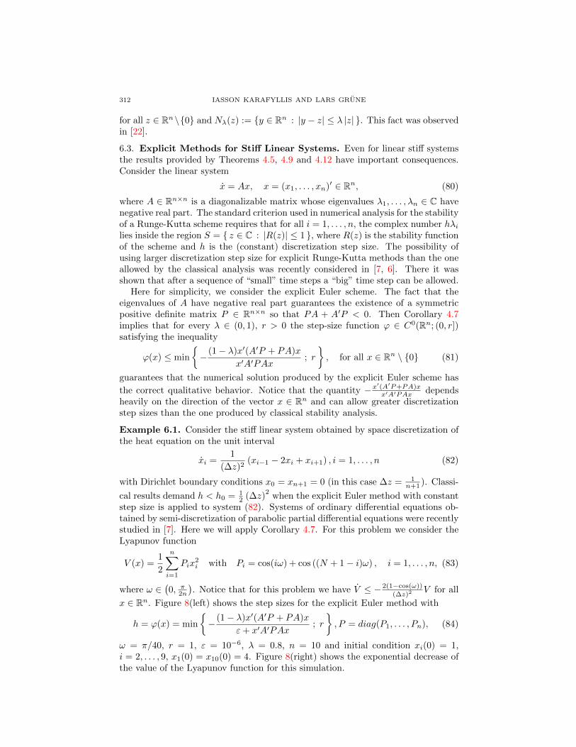
312 IASSON KARAFYLLIS AND LARS GRUNE
for all z ∈ Rn\0 and Nλ(z) := y ∈ Rn : |y − z| ≤ λ |z| . This fact was observedin [22].
6.3. Explicit Methods for Stiff Linear Systems. Even for linear stiff systemsthe results provided by Theorems 4.5, 4.9 and 4.12 have important consequences.Consider the linear system
x = Ax, x = (x1, . . . , xn)′ ∈ Rn, (80)
where A ∈ Rn×n is a diagonalizable matrix whose eigenvalues λ1, . . . , λn ∈ C havenegative real part. The standard criterion used in numerical analysis for the stabilityof a Runge-Kutta scheme requires that for all i = 1, . . . , n, the complex number hλilies inside the region S = z ∈ C : |R(z)| ≤ 1 , where R(z) is the stability functionof the scheme and h is the (constant) discretization step size. The possibility ofusing larger discretization step size for explicit Runge-Kutta methods than the oneallowed by the classical analysis was recently considered in [7, 6]. There it wasshown that after a sequence of “small” time steps a “big” time step can be allowed.
Here for simplicity, we consider the explicit Euler scheme. The fact that theeigenvalues of A have negative real part guarantees the existence of a symmetricpositive definite matrix P ∈ Rn×n so that PA + A′P < 0. Then Corollary 4.7implies that for every λ ∈ (0, 1), r > 0 the step-size function ϕ ∈ C0(Rn; (0, r])satisfying the inequality
ϕ(x) ≤ min
− (1− λ)x′(A′P + PA)x
x′A′PAx; r
, for all x ∈ Rn \ 0 (81)
guarantees that the numerical solution produced by the explicit Euler scheme has
the correct qualitative behavior. Notice that the quantity −x′(A′P+PA)xx′A′PAx depends
heavily on the direction of the vector x ∈ Rn and can allow greater discretizationstep sizes than the one produced by classical stability analysis.
Example 6.1. Consider the stiff linear system obtained by space discretization ofthe heat equation on the unit interval
xi =1
(∆z)2(xi−1 − 2xi + xi+1) , i = 1, . . . , n (82)
with Dirichlet boundary conditions x0 = xn+1 = 0 (in this case ∆z = 1n+1 ). Classi-
cal results demand h < h0 = 12 (∆z)
2when the explicit Euler method with constant
step size is applied to system (82). Systems of ordinary differential equations ob-tained by semi-discretization of parabolic partial differential equations were recentlystudied in [7]. Here we will apply Corollary 4.7. For this problem we consider theLyapunov function
V (x) =1
2
n∑i=1
Pix2i with Pi = cos(iω) + cos ((N + 1− i)ω) , i = 1, . . . , n, (83)
where ω ∈(0, π2n
). Notice that for this problem we have V ≤ − 2(1−cos(ω))
(∆z)2V for all
x ∈ Rn. Figure 8(left) shows the step sizes for the explicit Euler method with
h = ϕ(x) = min
− (1− λ)x′(A′P + PA)x
ε+ x′A′PAx; r
, P = diag(P1, . . . , Pn), (84)
ω = π/40, r = 1, ε = 10−6, λ = 0.8, n = 10 and initial condition xi(0) = 1,i = 2, . . . , 9, x1(0) = x10(0) = 4. Figure 8(right) shows the exponential decrease ofthe value of the Lyapunov function for this simulation.
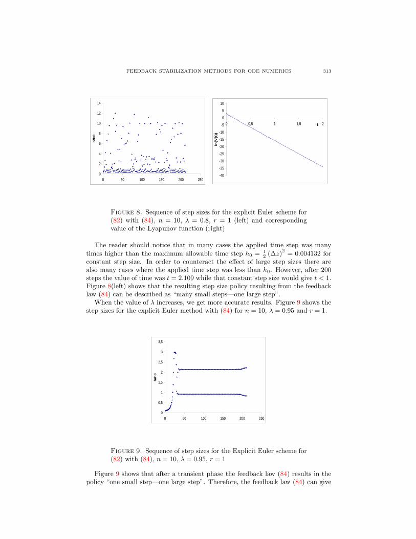
FEEDBACK STABILIZATION METHODS FOR ODE NUMERICS 313
0
2
4
6
8
10
12
14
0 50 100 150 200 250
h/h
0
-40
-35
-30
-25
-20
-15
-10
-5
0
5
10
0 0,5 1 1,5 2t
ln(V
(t))
Figure 8. Sequence of step sizes for the explicit Euler scheme for(82) with (84), n = 10, λ = 0.8, r = 1 (left) and correspondingvalue of the Lyapunov function (right)
The reader should notice that in many cases the applied time step was manytimes higher than the maximum allowable time step h0 = 1
2 (∆z)2
= 0.004132 forconstant step size. In order to counteract the effect of large step sizes there arealso many cases where the applied time step was less than h0. However, after 200steps the value of time was t = 2.109 while that constant step size would give t < 1.Figure 8(left) shows that the resulting step size policy resulting from the feedbacklaw (84) can be described as “many small steps—one large step”.
When the value of λ increases, we get more accurate results. Figure 9 shows thestep sizes for the explicit Euler method with (84) for n = 10, λ = 0.95 and r = 1.
0
0,5
1
1,5
2
2,5
3
3,5
0 50 100 150 200 250
h/h
0
Figure 9. Sequence of step sizes for the Explicit Euler scheme for(82) with (84), n = 10, λ = 0.95, r = 1
Figure 9 shows that after a transient phase the feedback law (84) results in thepolicy “one small step—one large step”. Therefore, the feedback law (84) can give
314 IASSON KARAFYLLIS AND LARS GRUNE
different step size policies for different values of λ. As expected, a trade-off betweenthe allowable time steps and the accuracy of the numerical solution exists. Forλ = 0.95, after 200 steps the value of time was t = 1.1956.
7. Conclusions. In this work, we considered the problem of step size selection fornumerical schemes such that the numerical solution presents the same qualitativebehavior as the original system of ODEs. Specifically, we developed tools for non-linear systems with a globally asymptotically stable equilibrium point which aresimilar to methods used in nonlinear control theory. It is shown how the problem ofappropriate step size selection can be converted to a rigorous abstract feedback sta-bilization problem for a particular hybrid system. Feedback stabilization methodsbased on Lyapunov functions and Small-Gain results were employed. The obtainedresults have been applied to several examples of applications including ODEs andsemi-discretized PDEs.
The methodology presented in the present work can be used for more complicatednumerical problems such as the step size selection problem for
(i) the numerical approximation of the solution of infinite-dimensional systems,i.e., systems governed by partial differential equations or systems describedby retarded functional differential equations
(ii) systems with more complicated attractors,(iii) time-varying systems(iv) systems with inputs.
Future work will address these problems.
Appendix A. Proofs from Section 4.1. In this appendix we provide the proofsof Lemma 4.3 and Proposition 4.4.Proof of Lemma 4.3. (i) Define Q(x) := −∇V (x)f(x). The function Q : Rn → R+
is continuous and by virtue of (37) it is positive definite, too. Standard results oninf-convolutions (see, e.g., [2, Section 3.5]) guarantee that the function W (x) :=inf Q(y) + |y − x| : y ∈ Rn is globally Lipschitz on Rn with Lipschitz constantL = 1, positive definite and satisfies (38).
(ii) Since f(0) = 0, for all x ∈ Rn it follows
|f(z)| ≤ lf (x) |z| for all z ∈ Rn with V (z) ≤ V (x). (85)
Inequality (85) in conjunction with the fact that V (z(t, x)) ≤ V (x) for all t ≥ 0 andGronwall’s inequality implies
exp (−lf (x) t) |x| ≤ |z(t, x)| ≤ exp (lf (x) t) |x| for all (t, x) ∈ R+ × Rn (86)
Therefore, (40) and inequality (86) imply
exp (−b) |x| ≤ |z(h, x)| ≤ exp (b) |x| for all h ∈ [0, ϕ(x)]. (87)
Let W : Rn → R+ be the locally Lipschitz, positive definite function which satisfiesinequality (38) and define
W (x) := min W (y) : y ∈ Rn , exp(−b) |x| ≤ |y| ≤ exp(b) |x| . (88)
Clearly, definition (88) guarantees that W : Rn → R+ is a continuous, positivedefinite function. Moreover, by virtue of inequalities (38), (87) and definition (88)

FEEDBACK STABILIZATION METHODS FOR ODE NUMERICS 315
we obtain for all h ∈ [0, ϕ(x)] and x ∈ Rn
V (z(h, x))− V (x) =
∫ h
0
∇V (z(s, x))f(z(s, x))ds ≤ −∫ h
0
W (z(s, x))ds ≤ −hW (x),
(89)i.e., (39).
(iii) Notice first that (41) guarantees the existence of ϕ ∈ C0(Rn; (0,+∞)) sat-isfying (42). Define
M bf (x) := max |f(y)| : y ∈ Rn , |y| ≤ exp(b) |x| . (90)
Inequality (85) and definition (90) imply
M bf (x) ≤ lf (x) exp(b) |x| . (91)
Taking into account inequalities (87), (91) and (42) in conjunction with definition(90) we obtain for all h ∈ [0, ϕ(x)] and x ∈ Rn
|W (x)−W (z(h, x))| ≤ lbW (x) |x− z(h, x)| ≤ lbW (x)lf (x) exp(b) |x|ϕ(x). (92)
Inequalities (92) and (42) imply
−W (z(h, x)) ≤ −λW (x) for all h ∈ [0, ϕ(x)] and all x ∈ Rn. (93)
Moreover, by virtue of inequalities (38), (87) and definition (88) we obtain
V (z(h, x))−V (x) =
∫ h
0
∇V (z(s, x))f(z(s, x))ds ≤ −∫ h
0
W (z(s, x))ds ≤ −λhW (x)
for all h ∈ [0, ϕ(x)] and all x ∈ Rn, i.e., the assertion. This finishes the proof.
Proof of Proposition 4.4. Since the origin 0 ∈ Rn is locally exponentially stablefor (1), it follows that the matrix A := Df(0) has only eigenvalues with negativereal part. Consequently there exists a symmetric, positive definite matrix P ∈ Rn×nand a constant µ > 0 such that
x′(A′P + PA)x ≤ −2µ |x|2 for all x ∈ Rn, (94)
see [34]. Consequently, for sufficiently small δ > 0 we obtain
2x′Pf(x) ≤ −µ |x|2 for all x ∈ Rn with |x| ≤ 2δ. (95)
Let W : Rn → R+ a continuously differentiable function with
W (x) :=
−2x′Pf(x), |x| < δ
µ |x|2(
1 + |f(x)|2), |x| > 2δ
and W (x) ≥ µ |x|2 for all x ∈ Rn
(96)and define the function
V (x) :=
∫ +∞
0
W (z(t, x))dt. (97)
By virtue of Theorem 2.46 in [8], V as defined by (97) is a Lyapunov function for(1) satisfying
∇V (x)f(x) = −W (x) for all x ∈ Rn. (98)
From Proposition 2.48 in [8] it follows that V is the unique function satisfying(98) with V (0) = 0. An inspection of the proof of this proposition yields that ifequation (98) holds on a forward invariant set for (1) then uniqueness holds on thisset, because uniqueness is established by looking at trajectories in forward time.Furthermore, by virtue of (98) and definition (96) it follows that (44) holds.

316 IASSON KARAFYLLIS AND LARS GRUNE
Now we pick a forward invariant neighborhood N ⊂ Bδ(0) of zero which existsbecause 0 ∈ Rn is asymptotically stable. Then we observe by (96) that the function
V (x) = x′Px satisfies (98) as well on N ⊂ Bδ(0) and V (0) = 0. Consequently,
V (x) ≡ V (x) = x′Px on N ⊂ Bδ(0). Thus, for ε > 0 sufficiently small such thatBε(0) ⊆ N , it follows that (43) holds.
REFERENCES
[1] Z. Artstein, Stabilization with relaxed controls, Nonlinear Anal., 7 (1983), 1163–1173.
[2] P. Cannarsa and C. Sinestrari, “Semiconcave Functions, Hamilton-Jacobi Equations, and
Optimal Control,” Progress in Nonlinear Differential Equations and their Applications, 58,Birkhauser Boston Inc., Boston, MA, 2004.
[3] S. Dashkovskiy, B. S. Ruffer and F. R. Wirth, An ISS small gain theorem for general networks,
Math. Control Signals Systems, 19 (2007), 93–122.[4] R. A. Freeman and P. V. Kokotovic, “Robust Nonlinear Control Design – State-Space and
Lyapunov Techniques,” Birkhauser, Boston, MA, 1996.
[5] B. M. Garay and K. Lee, Attractors under discretization with variable stepsize, DiscreteContin. Dyn. Syst., 13 (2005), 827–841.
[6] C. W. Gear and I. G. Kevrekidis, Projective methods for stiff differential equations: Problemswith gaps in their eigenvalue spectrum, SIAM J. Sci. Comput., 24 (2003), 1091–1106.
[7] C. W. Gear and I. G. Kevrekidis, Telescopic projective methods for parabolic differential
equations, J. Comput. Phys., 187 (2003), 95–109.[8] P. Giesl, “Construction of Global Lyapunov Functions Using Radial Basis Functions,” volume
1904 of “Lecture Notes in Mathematics,” Springer, Berlin, 2007.
[9] B. S. Goh, Algorithms for unconstrained optimization problems via control theory, J. Optim.Theory Appl., 92 (1997), 581–604.
[10] V. Grimm and G. R. W. Quispel, Geometric integration methods that preserve Lyapunov
functions, BIT, 45 (2005), 709–723.[11] L. Grune, “Asymptotic Behavior of Dynamical and Control Systems under Perturbation and
Discretization,” volume 1783 of “Lecture Notes in Mathematics,” Springer, Berlin, 2002.
[12] L. Grune, Attraction rates, robustness, and discretization of attractors, SIAM J. Numer.Anal., 41 (2003), 2096–2113.
[13] L. Grune, E. D. Sontag and F. R. Wirth, Asymptotic stability equals exponential stability,and ISS equals finite energy gain—if you twist your eyes, Syst. Control Lett., 38 (1999),
127–134.
[14] K. Gustafsson, Control-theoretic techniques for stepsize selection in explicit Runge-Kuttamethods, ACM Trans. Math. Software, 17 (1991), 533–554.
[15] K. Gustafsson, Control-theoretic techniques for stepsize selection in implicit Runge-Kuttamethods, ACM Trans. Math. Software, 20 (1994), 496–517.
[16] K. Gustafsson, M. Lundh and G. Soderlind, A PI stepsize control for the numerical solution
of ordinary differential equations, BIT, 28 (1988), 270–287.
[17] E. Hairer, C. Lubich and G. Wanner, “Geometric Numerical Integration. Structure-PreservingAlgorithms for Ordinary Differential Equations,” Springer, Berlin, second edition, 2006.
[18] E. Hairer, S. P. Nørsett and G. Wanner, “Solving Ordinary Differential Equations. I NonstiffProblems,” Springer, Berlin, second edition, 1993.
[19] E. Hairer and G. Wanner, “Solving Ordinary Differential Equations. II Stiff and Differential-
Algebraic Problems,” Springer, Berlin, second edition, 1996.[20] Z.-P. Jiang, A. R. Teel and L. Praly, Small-gain theorem for ISS systems and applications,
Math. Control Signals Systems, 7 (1994), 95–120.
[21] I. Karafyllis, Non-uniform robust global asymptotic stability for discrete-time systems andapplications to numerical analysis, IMA J. Math. Control Inform., 23 (2006), 11–41.
[22] I. Karafyllis, A system-theoretic framework for a wide class of systems. I, Applications to
numerical analysis, J. Math. Anal. Appl., 328 (2007), 876–899.[23] I. Karafyllis and Z.-P. Jiang, A small-gain theorem for a wide class of feedback systems with
control applications, SIAM J. Control Optim., 46 (2007), 1483–1517.
[24] I. Karafyllis and Z.-P. Jiang, A vector small-gain theorem for general nonlinear control sys-tems, In “Proceedings of the 48th IEEE Conference on Decision and Control,” pages 7996–
8001, Shanghai, China, 2009. arXiv:0904.0755.
FEEDBACK STABILIZATION METHODS FOR ODE NUMERICS 317
[25] H. K. Khalil, “Nonlinear Systems,” Prentice Hall, Upper Saddle River, third edition, 2002.[26] P. E. Kloeden and J. Lorenz, Stable attracting sets in dynamical systems and in their one-step
discretizations, SIAM J. Numer. Anal., 23 (1986), 986–995.
[27] P. E. Kloeden and B. Schmalfuss, Lyapunov functions and attractors under variable time-stepdiscretization, Discrete Contin. Dynam. Systems, 2 (1996), 163–172.
[28] V. Lakshmikantham and D. Trigiante, “Theory of Difference Equations: Numerical Methodsand Applications,” Marcel Dekker, New York, second edition, 2002.
[29] H. Lamba, Dynamical systems and adaptive timestepping in ODE solvers, BIT, 40 (2000),
314–335.[30] Y. Lin, E. D. Sontag and Y. Wang, A smooth converse Lyapunov theorem for robust stability,
SIAM J. Control Optim., 34 (1996), 124–160.
[31] J. Peng, Z.-B. Xu, H. Qiao and B. Zhang, A critical analysis on global convergence of Hopfield-type neural networks, IEEE Trans. Circuits Syst. I Regul. Pap., 52 (2005), 804–814.
[32] E. D. Sontag, Smooth stabilization implies coprime factorization, IEEE Trans. Automat.
Control, 34 (1989), 435–443.[33] E. D. Sontag, A “universal” construction of Artstein’s theorem on nonlinear stabilization,
Systems Control Lett., 13 (1989), 117–123.
[34] E. D. Sontag, “Mathematical Control Theory,” Springer, New York, second edition, 1998.[35] A. M. Stuart and A. R. Humphries, “Dynamical Systems And Numerical Analysis,” Cam-
bridge University Press, Cambridge, 1996.[36] A. R. Teel, Input-to-state stability and the nonlinear small gain theorem, Preprint, 2005.
[37] Y. Xia and J. Wang, A recurrent neural network for nonlinear convex optimization subject
to nonlinear inequality constraints, IEEE Trans. Circuits Syst., 51 (2004), 1385–1394.[38] H. Yamashita, A differential equation approach to nonlinear programming, Math. Program-
ming, 18 (1980), 155–168.
[39] L. Zhou, Y. Wu, L. Zhang and G. Zhang, Convergence analysis of a differential equationapproach for solving nonlinear programming problems, Appl. Math. Comput., 184 (2007),
789–797.
Received May 2010; revised August 2010.
E-mail address: [email protected]
E-mail address: [email protected]