Feedback Control Law for Variable Speed Control Moment...

Feedback Control Law for VariableSpeed Control Moment Gyros

Hanspeter Schaub , Srinivas R. Vadali and John L. Junkins

Simulated Reprint from

Journal of the Astronautical SciencesVol. 46, No. 3, July–Sept., 1998, Pages 307–328

A publication of theAmerican Astronautical SocietyAAS Publications OfficeP.O. Box 28130San Diego, CA 92198

Journal of the Astronautical Sciences Vol. 46, No. 3, July–Sept., 1998, Pages 307–328

Feedback Control Law for VariableSpeed Control Moment Gyros

Hanspeter Schaub∗, Srinivas R. Vadali† and John L. Junkins‡

Abstract

Variable speed control moment gyroscopes are single-gimbal gyroscopes where the fly wheel speed is allowedto be variable. The equations of motion of a generic rigid body with several such variable speed CMGsattached. The formulation is such that it can easily accommodate the classical cases of having either controlmoment gyros or reaction wheels to control the spacecraft attitude. A globally asymptotically stabilizingnonlinear feedback control law is presented. For a redundant control system, a weighted minimum norminverse is used to determine the control vector. This approach allows the variable speed control momentgyroscopes to behave either more like classical reaction wheels or more like control moment gyroscopes,depending on the local optimal steering logic. Where classical control moment gyroscope control laws haveto deal with singular gimbal angle configurations, the variable speed control moment gyroscopes are shownnot to encounter any singularities for many representative examples considered. Both a gimbal angle velocityand an acceleration based steering law are presented. Further, the use of the variable speed CMG null motionis discussed to reconfigure the gimbal angles to preferred sets. Having a variable reaction wheel speed allowsfor a more general redistribution of the internal momentum vector.

Introduction

Instead of using thrusters to perform precise spacecraft attitude maneuvers, usually control mo-ment gyros (CMGs) or reaction wheels (RWs) are used. A single-gimbal CMG contains a wheelspinning at a constant rate. To exert a torque onto the spacecraft this wheel is gimbaled or rotatedabout a body-fixed axis.1,2, 3 The rotation axis and rotation angle are referred to as the gimbal axisand gimbal angle respectively. A separate feedback control loop is used to spin up the rotor to therequired spin rate and maintain it. The advantage of a CMG is that a relatively small gimbal torqueinput is required to produce a large effective torque output on the spacecraft. This makes a clusterof CMGs a very popular choice for reorienting large space structures such as the space station orSkylab. The drawback of the single-gimbal CMGs is that their control laws can be fairly complexand that such CMG systems encounter certain singular gimbal angle configurations. At these singu-lar configurations the CMG cluster is unable to produce the required torque exactly, or any torqueat all if the required torque is orthogonal to the plane of allowable torques. Several papers deal withthis issue and present various solutions.4,1, 2, 3 However, even with singularity robust steering laws orwhen various singularity avoidance strategies are applied, the actual torque produced by the CMGcluster is never equal to the required torque when maneuvering in the proximity of a singularity.

∗Graduate Research Assistant, Aerospace Engineering Department, Texas A&M University, College Station TX 77843.†Professor, Department of Aerospace Engineering, Texas A&M University, College Station, TX 77843.‡George J. Eppright Distinguished Chair Professor of Aerospace Engineering, Aerospace Engineering Department, Texas

A&M University, College Station TX 77843, Fellow AAS.

1

2 Schaub, Vadali and Junkins

The resulting motion may be stable, but these path deviations can be highly undesirable in someapplications.

Reaction wheels (RWs), on the other hand, have a wheel spinning about a body fixed axis whosespin speed is variable. Torques are produced on the spacecraft by accelerating or decelerating thereaction wheels.5,6 RW systems don’t have singular configurations and typically have simpler controllaws than CMG clusters. Drawbacks to the reaction wheels include a relatively small effective torquebeing produced on the spacecraft and the possibility of reaction wheel saturation. To exert a giventorque onto a spacecraft, reaction wheels typically require more energy than CMGs.

Variable Speed Control Moment Gyroscopes (VSCMGs) combine positive features of both thesingle-gimbal CMGs and the RWs. The spinning disk can be rotated or gimbaled about a singlebody fixed axis, while the disk spin rate is also free to be controlled.7 This adds an extra degreeof control to the classical single-gimbal CMG device. Note that adding this variable speed featurewould not require the single-gimbal CMG to be completely reengineered. These devices already havea separate feedback loop that maintains a constant spin rate. What might need to be changed is thetorque motor controlling the RW spin rate, which would need to be stronger, and the constant speedRW feedback law, which would be abandoned. With this extra control, singular configurations, in theclassical CMG sense, will not be present. Because CMGs are known to be more efficient energy wisethan RWs, away from a classical single-gimbal CMG singular configuration, the VSCMG steeringlaw will ideally act like the classical CMG steering law. As a single-gimbal CMG singularity isapproached, the VSCMGs should begin to act more like RWs to avoid the excessive torques thatwould normally occur and ensure that the applied torque of the VSCMG cluster is exactly equalto the required torque. This strategy will allow for precise steering without path deviations nearclassical CMG singularities because the actual commanded torque will be generated at all times.In this paper, both a gimbal velocity based and an gimbal acceleration based steering law will bepresented. Lyapunov analysis will be used to guarantee global asymptotic stability of the feedbackcontrol law. Further, the use of the VSCMG null motion to reconfigure the gimbal angles and modifythe RW spin speed is discussed. Having a variable speed RW allows for this to be done in a muchmore general manner. The torque required of these types of maneuvers and whether they could bedone with existing CMG hardware will be investigated.

Equations of Motion

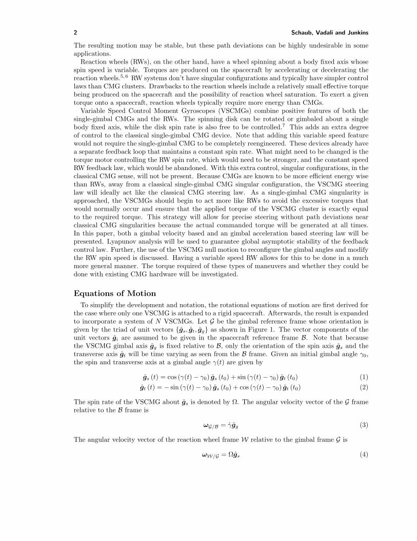
To simplify the development and notation, the rotational equations of motion are first derived forthe case where only one VSCMG is attached to a rigid spacecraft. Afterwards, the result is expandedto incorporate a system of N VSCMGs. Let G be the gimbal reference frame whose orientation isgiven by the triad of unit vectors gs, gt, gg as shown in Figure 1. The vector components of theunit vectors gi are assumed to be given in the spacecraft reference frame B. Note that becausethe VSCMG gimbal axis gg is fixed relative to B, only the orientation of the spin axis gs and thetransverse axis gt will be time varying as seen from the B frame. Given an initial gimbal angle γ0,the spin and transverse axis at a gimbal angle γ(t) are given by

gs (t) = cos (γ(t)− γ0) gs (t0) + sin (γ(t)− γ0) gt (t0) (1)gt (t) = − sin (γ(t)− γ0) gs (t0) + cos (γ(t)− γ0) gt (t0) (2)

The spin rate of the VSCMG about gs is denoted by Ω. The angular velocity vector of the G framerelative to the B frame is

ωG/B = γgg (3)

The angular velocity vector of the reaction wheel frame W relative to the gimbal frame G is

ωW/G = Ωgs (4)

Feedback Control Law for Variable Speed Control Moment Gyros 3

Ω

γ

gt

gs

gg

Figure 1: Illustration of a Variable Speed Control Moment Gyroscope

To indicate in which reference frame vector or matrix components are taken, a superscript letteris added before the vector or matrix name. Because the G frame unit axes are aligned with theprincipal gimbal frame axes, the gimbal frame inertia matrix [IG] expressed in the G frame is theconstant diagonal matrix.

[IG] = G [IG] = diag(IGs, IGt

, IGg) (5)

where IGs, IGt

and IGgare the gimbal frame inertias about the corresponding spin, transverse and

gimbal axes. The reaction wheel inertia about the same axes are denoted by IWs, IWt

and IWt.

[IW ] = W [IW ] = diag(IWs , IWt , IWt) (6)

Note that since the disk is symmetric about the gs axis W [IW ] = G [IW ]. In practice IWsis typically

much larger than any of the other gimbal frame or RW inertias. In this development the RW andgimbal frame inertias are not combined early on into one overall VSCMG inertia matrix; rather,they are retained as separate entities until later into the development. This will allow for a preciseformulation of the actual physical motor torques that drive the RWs or the CMGs.

The G frame orientation is related to the B frame orientation through the direction cosine matrix[BG] which is expressed in terms of the gimbal frame unit direction vectors as

[BG] = [gs gt gg] (7)

In Eq. (7) the gi vector components are taken in the B frame. The rotation matrix [BG] maps avector with components taken in the G frame into a vector with components in the B frame. Theconstant diagonal inertia matrices G [IG] and G [IW ] are expressed with components taken in the Bframe as the time varying matrices8,9

B[IG] = [BG] G [IG] [BG]T = IGs gsgTs + IGt gtg

Tt + IGg ggg

Tg (8)

B[IW ] = [BG] G [IW ] [BG]T = IWs gsgTs + IWt gtg

Tt + IWt ggg

Tg (9)

The total angular momentum of the spacecraft and the VSCMG about the spacecraft center ofmass is given by

H = HB + HG + HW (10)


where HB is the angular momentum component of the spacecraft, HG is the angular momentumof the gimbal frame and HW is the angular momentum of the RW. Let N be an inertial referenceframe and ωB/N be the relative angular velocity vector, then HB is written as

HB = [Is]ωB/N (11)

The matrix [Is] contains the spacecraft inertias and the VSCMG inertia components due to the factthat the VSCMG center of mass is not located at the spacecraft center of mass. Note that B[Is] isa constant matrix as seen from the B frame. The gimbal frame angular momentum HG is given by

HG = [IG]ωG/N (12)

where ωG/N = ωG/B + ωB/N . Using Eqs. (3), (5) and (8) this is rewritten as

HG =(IGs gsg

Ts + IGt gtg

Tt + IGg ggg

Tg

)ωB/N + IGg γgg (13)

To simplify the following notation, let the variables ωs, ωt and ωg be the projection of ωB/N ontothe G frame unit axes.

ωs = gTs ωB/N ωt = gT

t ωB/N ωg = gTg ωB/N (14)

The angular momentum HG is then written as

HG = IGsωsgs + IGt

ωtgt + IGg(ωg + γ) gg (15)

The RW angular momentum HW is given by

HW = [IW ]ωW/N (16)

where ωW/N = ωW/G + ωG/B + ωB/N . Using analogous definitions as for HG, HW is rewritten as

HW = IWs(ωs + Ω) gs + IWt

ωtgt + IWt(ωg + γ) gg (17)

To simplify the notation from here on, let us use the short hand notation ω = ωB/N . In somecalculations it will be convenient to express ω in the G frame as

Gω = ωsgs + ωtgt + ωggg (18)

To denote that a vector x is being differentiated relative to a reference frame A, the followingnotation is used.

Ad

dt(x)

Indicating an inertial time derivatives of a vector x will be abbreviated as

Nd

dt(x) ≡ x

The equations of motion of a system of rigid bodies follow from Euler’s equation8,9

H = L (19)

if all moments are taken about the center of mass. The vector L represents the sum of all the externaltorques experienced by the spacecraft. The time derivative of HW is expressed as expressed as

HW = gsIWs

(Ω + gT

s ω + γωt

)+ gt

(IWs

γωs + IWtgT

t ω + (IWs− IWt

) ωsωg + IWsΩ (γ + ωg)

)+ gg

(IWt

gTg (ω + γ) + (IWt

− IWs)ωsωt + IWs

Ωωt

) (20)


Let LW be the torque the gimbal frame exerts on the RW. Euler’s equation for the RW is HW =LW . The torque components in the gt and gg direction are produced by the gimbal frame itself.However, the torque component us about the gs axis is produced by the RW torque motor. Therefore,from Eq. (20) the spin control torque us is given by

us = IWs

(Ω + gT

s ω + γωt

)(21)

Differentiating Eq. (15), the momentum rate HG is written as

HG = gs

((IGs

− IGt+ IGg

)γωt + IGs

gTs ω +

(IGg

− IGt

)ωtωg

)+ gt

((IGs

− IGt− IGg

)γωs + IGt

gTt ω + (IGs

− IGt) ωsωg

)+ gg

(IGg

(gT

g ω + γ)

+ (IGt − IGs) ωsωt

) (22)

From here on it is convenient to combine the inertia matrices of the RW and the gimbal frame intoone VSCMG inertia matrix [J ] as

[J ] = [IG] + [IW ] = diag(Js, Jt, Jg) (23)

Let LG be the torque vector that the combined RW and CMG system exerts onto the spacecraft,then Euler’s equation states that HG + HW = LG. The LG torque component about the gg axis isproduced by the gimbal torque motor. Adding Eqs. (20) and (22) and making use of the definitionin Eq. (23), the gimbal torque ug is then expressed as

ug = Jg

(gT

g ω + γ)− (Js − Jt)ωsωt − IWs

Ωωt (24)

The inertial derivative of HB is simply

HB = [Is]ω + [ω][Is]ω (25)

where the tilde matrix operator [ω] is defined as

[ω] =

0 −ω3 ω2

ω3 0 −ω1

−ω2 ω1 0

(26)

To further simplify the equations of motions, we define the total spacecraft inertia matrix [I] as

[I] = [Is] + [J ] (27)

Substituting Eqs. (20), (22) and (25) back into Eq. (19) and making use of the definition in Eq. (27),we find the equations of motion for a rigid spacecraft containing one VSCMG.

[I]ω = −[ω][I]ω − gs

(Jsγωt + IWs

Ω− (Jt − Jg)ωtγ)

− gt ((Jsωs + IWsΩ) γ − (Jt + Jg) ωsγ + IWsΩωg)− gg (Jgγ − IWsΩωt) + L

(28)

At this point, we make the common assumption that Js ≈ IWs , i.e,. that the gimbal frame inertiaIGs about the spin axis is negligible. The corresponding equations of motion are simplified to

[I]ω = −[ω][I]ω − gs

(Js

(Ω + γωt

)− (Jt − Jg) ωtγ

)− gt (Js (ωs + Ω) γ − (Jt + Jg) ωsγ + JsΩωg)− gg (Jgγ − JsΩωt) + L

(29)


To obtain the equations of motion of a rigid spacecraft with several VSCMGs attached, we addthe effects of each HG and HW . To simplify notation, let us define the following useful matrices.The matrices [Gs], [Gt] and [Gg] contain the unit direction vectors of each VSCMG gimbal frame.

[Gs] = [gs1 · · · gsN] [Gt] = [gt1 · · · gtN

] [Gg] = [gg1 · · · ggN] (30)

The total spacecraft inertia matrix is expressed as

[I] = [Is] +N∑

i=1

[Ji] = [Is] +N∑

i=1

Jsi gsi gTsi

+ Jti gti gTti

+ Jgi ggi gTgi

(31)

The effective torque quantities τsi , τti and τgi are defined as

τs =

Js1

(Ω1 + γ1ωt1

)− (Jt1 − Jg1) ωt1 γ1

...JsN

(ΩN + γNωtN

)− (JtN

− JgN) ωtN

γN

(32a)

τs =

Js1 (Ω1 + ωs1) γ1 − (Jt1 + Jg1) ωs1 γ1 + Js1Ω1ωg1

...JsN

(ΩN + ωsN) γN − (JtN

+ JgN) ωsN

γN + JsNΩNωgN

(32b)

τg =

Jg1 γ1 − Js1Ω1ωt1...

JgNγN − JsN

ΩNωtN

(32c)

The rotational equations of motion for a rigid body containing N VSCMGs are then written com-pactly as

[I]ω = −[ω][I]ω − [Gs]τs − [Gt]τt − [Gg]τg + L (33)

Also, The rotational kinetic energy T of a rigid spacecraft with N VSCMGs is given by

T =12ωT [Is]ω +

12

N∑i=1

Jsi(Ωi + ωsi

)2 + Jtiω2

ti+ Jgi

(ωgi+ γi)

2 (34)

The kinetic energy or work rate, found after differentiating Eq. (34) with respect to time andperforming some lengthy algebra, is found to be

T =N∑

i=1

γiugi + Ωiusi + ωT L (35)

Actually, the energy rate expression for this system of rigid bodies was known apriori from the Work-Energy-Rate principle.10 Hence, the derivation of Eq. (35) from the equations of motion validatesthe equations of motion.

Feedback Control Law

In this section, a feedback law is derived using Lyapunov control theory. Given some initialangular velocity and attitude measure, the goal of the control law is to bring the rigid body to restat the zero attitude (aligned with the reference frame). The attitude coordinate system is chosensuch that the zero attitude is the desired attitude. To describe the rigid spacecraft attitude, thispaper uses the very elegant set of recently developed Modified Rodrigues Parameters (MRP) alongwith their “shadow” counterparts.11,12,13,14,15,16 They allow for a non-singular rigid body attitude


description with several other useful attributes. The MRPs can be defined in terms of the Eulerparameters β as11,13,16

σi =βi

1 + β0i = 1,2,3 (36)

Or, in terms of the principal rotation axis e and the principal rotating angle φ, the MRP vector is

σ = e · tan(φ/4) (37)

Note that the tangent function typically behaves very linearly for angles up to 20 degrees. SinceEq. (37) shows that σ is written in terms of tan(φ/4), the MRPs behave very linearly for principalrotations up to ±80 degrees. This is a much larger range of rotations that can be assumed to behavenear-linearly than what can be typically achieved using standard Euler Angles or even the classicalRodrigues parameters.

Like the Euler parameters, the modified Rodrigues parameters are not unique. A second set ofmodified Rodrigues parameters, called the “shadow” set, can be used to avoid the singularity of the“original” MRP at φ = ±360 at the cost of a discontinuity at a switching point. The transformationbetween the “original” and “shadow” sets of MRPs for any arbitrary switching surface σT σ =constant is11,17,15

σS = − σ

σT σ(38)

Typically the MRP vector σ is switched to it’s alternate set whenever σT σ > 1 which correspondsto the rigid body having tumbled past φ = ±180 degrees. The MRP differential kinematic equationonly contains a quadratic nonlinearity and is given by

dσ

dt=

12

[[I3×3]

(1− σT σ

2

)+ [σ] + σσT

]ωB/N (39)

where [I3x3] is a 3x3 identity matrix. In designing the control law, we assume that estimates ofω, σ, Ωi and γi are available. The following Lyapunov function V is a positive definite, radiallyunbounded measure of the total system state error relative to the target state ω = σ = 0 where Kis a scalar attitude feedback gain.6

V (ω,σ) =12ωT [I]ω + 2K log

(1 + σT σ

)(40)

The use of the logarithm function in this context was first introduced by Tsiotras in Ref. 13 and leadsto a control law which is linear in σ. Using Eqs. (14) and (31) the Lyapunov function is rewritten as

V =12ωT [Is]ω +

12

N∑i=1

(Jsiω

2si

+ Jtiω2ti

+ Jgiω2gi

)+ 2K log

(1 + σT σ

)(41)

Differentiating the Lyapunov function V yields

V = ωT

([I]ω +

N∑i=1

(Jsi− Jti

) γiωtigsi

+ Kσ

)(42)

Lyapunov stability theory requires that V be negative semi-definite to guarantee stability. Let [P ]be a positive definite angular velocity feedback gain matrix, then V is set to be

V = −ωT [P ]ω (43)


which, when combined with Eq. (42), leads to the following condition for stability.

[I]ω = −Kσ − [P ]ω −N∑

i=1

(Jsi − Jti) γiωti gsi (44)

After substituting the equations of motion given in Eq. (33) into Eq. (44) and simplifying the result,the following stability requirement is obtained.

N∑i=1

(gsi

JsiΩi + ggi

Jgiγi + gti

(Jsi(Ωi + ωsi

)− Jtiωsi

) γi

)= Kσ + [P ]ω + L (45)

To express this condition in a more compact and useable form, let us define the following 3xNmatrices.

[D0] = [gs1Js1 · · · gsNJsN

] (46a)[D1] = [gt1Js1 (Ω1 + ωs1) · · · gtN

JsN(ΩN + ωsN

)] (46b)[D2] = [gt1Jt1ωs1 · · · gtN

JtNωsN

] (46c)[B] = [gg1Jg1 · · · ggN

JgN] (46d)

Let Ω, γ and γ be Nx1 vectors whose i-th element contains the respective VSCMG angular velocityor acceleration or RW spin rate. Then the stability condition in Eq. (45) is

[D0]Ω + [B]γ + ([D1]− [D2]) γ = Lr (47)

where Lr = Kσ + [P ]ω + L is called the required control torque. Dropping the [D0]Ω term, thestandard single-gimbal CMG stability condition is retrieved as it is developed in Ref. 1. Note thatthe condition in Eq. (47) only guarantees global stability in the sense of Lyapunov for the states ωand σ because V in Eq. (43) is only negative semi-definite, not negative definite. However, Eq. (43)does show that ω → 0 as time goes to infinity. To prove that the stability condition in Eq. (47)guarantees asymptotic stability of all states including σ, the higher order time derivatives of V mustbe investigated. A sufficient condition to guarantee asymptotic stability is that the first nonzerohigher-order derivative of V , evaluated on the set of states such that V is zero, must be of odd orderand be negative definite.18,19,20 For this dynamical system V is zero when ω is zero. DifferentiatingEq. (43), the second derivative of V is

d2

dt2V = −2ωT [P ]ω (48)

which is zero on the set of states where ω is zero. Differentiating again, the third derivative of V is

d3

dt3V = −2ωT [P ]ω − 2ωT [P ]ω (49)

By substituting Eq. (44) and setting ω = 0, we may express the third derivative of the Lyapunovfunction as

d3

dt3V = −K2σT

([I]−1

)T[P ][I]−1σ (50)

which is a negative definite quantity because both [I] and [P ] are positive definite matrices. Thereforethe stability condition in Eq. (47) does guarantee global asymptotic stability.


Velocity Based Steering Law

Note that the stability condition in Eq. (47) does not contain the physical control torques usi

and ugiexplicitly. Instead only gimbal rates and accelerations and RW accelerations appear. This

will lead to a steering law that determines the required time history of γ and Ω such that Eq. (47)is satisfied. The reason for this is two fold. First, commercial CMGs typically require γ as theinput, not the actual physical torque vector ug. Secondly, writing Eq. (47) in terms of the torquevectors us and ug and then solving for these would lead to a control law that is equivalent to solvingEq. (47) directly for γ. As has been pointed out in Ref. 1, this leads to a very undesirable controllaw with excessive gimbal rates. A physical reason for this is that such control laws provide therequired control torque mainly through the [B]γ term. In this setup the CMGs are essentially beingused as RWs and the potential torque amplification effect in not being exploited. Because CMGgimbal inertias Jg are typically very small compared to their spin inertia Js, the corresponding [B]will also be very small which leads to very large γ vectors.

To take advantage of the potential torque amplification effect, most of the required control torquevector Lr should be produced by the ([D1]− [D2]) γ term. This is why classical CMG steering lawscontrol primarily the γ vector and not γ. For the VSCMGs it is desirable to have the required torqueLr be produced by a combination of the Ω and γ terms in Eq. (47). Paralleling the developmentof the classical single-gimbal CMG velocity steering laws, the terms containing the transverse andgimbal VSCMG inertias are ignored at this level. Eq. (47) then becomes

[D0]Ω + [D1]γ = Lr (51)

Comparing the [D1] matrix to that of standard CMG steering laws it is evident that an extragtJsωs term is present in the VSCMG formulation. This term is also dropped in the standard CMGformulation because it can be assumed that ωs will typically be much smaller than Ω. However,since for a VSCMG the RW spin speed Ω is variable, this assumption can no longer be justified andthis term is retained in this formulation.

For notational convenience, we introduce the 2Nx1 state vector η

η =[Ωγ

](52)

and the 3x2N matrix [Q]

[Q] =[D0

... D1

](53)

Eq. (51) can then be written compactly as

[Q]η = Lr (54)

Note that each column of the [D0] matrix is a scalar multiple of the gsi vectors, while each columnof [D1] is a scalar multiple of the gti

vectors. In the classical 4 single-gimbal CMG cluster, singulargimbal configurations are encountered whenever the rank of [D1] is less than 3. This occurs wheneverthe gti

no longer span the three-dimensional space but form a plane. If this occurs, any requiredtorque which does not lie perfectly in this plane is not generated exactly by the CMG cluster and thespacecraft deviates slightly from the desired attitude. If the required control torque is perpendicularto this plane, then the CMG cluster produces no effective torque on the spacecraft. These singularconfigurations can never occur with a VSCMG because the rank of the [Q] matrix will never beless than 3! Since the gsi

vectors are perpendicular to the gtivectors, even when all the transverse

axes are coplanar, there will always be at least one spin axis that is not in this plane. Thereforethe columns of [Q] will always span the entire three-dimensional space as long as at least 2 or moreVSCMGs are used with unique ggi vectors.

Because the [Q] matrix is never rank deficient, a minimum norm solution for η can be obtainedusing the standard Moore-Penrose inverse. However, because ideally the VSCMGs are to act like


classical CMGs away from single-gimbal CMG singular configurations, a weighted pseudo inverse isused instead.21 Let [W ] be a 2Nx2N diagonal matrix

[W ] = diagWs1 , . . . , WsN,Wg1 , . . . , WgN

(55)

where Wsiand Wgi

are the weights associated with how nearly the VSCMGs are to perform likeregular RWs or CMGs. Then, the desired η is

η =[Ωγ

]= [W ][Q]T

([Q][W ][Q]T

)−1Lr (56)

Note that there is no need here to introduce a modified pseudo-inverse as Nakamura and Hanafusadid in developing the singularity robustness steering law in Ref. 22. To achieve the desired VSCMGbehavior, the weights are made dependent on the proximity to a single-gimbal CMG singularity. Tomeasure this proximity the scalar factor δ is defined as

δ = det([D1][D1]T

)(57)

As the gimbal angles approach a singular CMG configuration this parameter δ will go to zero. Theweights Wsi

are then defined to be

Wsi = W 0si

e(−µδ) (58)

where W 0si

and µ are positive scalars to be chosen by the control designer. The gains Wgiare

simply held constant. Away from CMG singularities this steering law will have very small weightson the RW mode and essentially perform like a classical single-gimbal CMG. As a singularity isapproached, the steering law will start to use the RW mode to ensure that the gimbal rates donot become excessive and that the required control torque Lr is actually produced by the VSCMGcluster.

Two types of CMG singularities are commonly discussed. The simpler type of singularity is whenthe rank of the [D1] matrix drops below 3 which is indicated by δ, defined in Eq. (57), approachingor becoming zero. The VSCMG velocity steering law in Eq. (56) handles temporary rank deficienciesvery well. The required control torque is always produced correctly by making use of the additioncontrol authority provided by the RW modes. Another type of singularity is when the requiredcontrol torque is exactly perpendicular to the span of the transverse VSCMG axis (i.e. Lr is in thenullspace of [D1]). Naturally, this is only possible whenever δ is zero. To measure how close therequired torque Lr is to the nullspace of [D1] the orthogonality index O is used.1

O =LT

r [D1]T [D1]Lr

||Lr||2(59)

Whenever Lr becomes part of the nullspace of [D1], then O will tend towards zero. A classicalsingle-gimbal CMG steering law demands a zero γ vector with this type of singularity which “locksup” the gimbals produces no effective torque on the spacecraft. The VSCMG steering does notprevent the gimbals from being locked up in these singular orientations; however, the Lr vector isstill being produced thanks to the RW mode of the VSCMGs. If a gimbal lock is actually achieved,then without any further changes, such as a change in the required Lr, the VSCMG will simplycontinue the maneuvers acting like pure RWs. Running numerical simulations it was found thatunless one starts the simulation in a pure gimbal lock situation, it was very unlikely for the VSCMGsteering law to lock up the gimbals. Once a singularity is approached, the RWs are spun up ordown which also in return affects the gimbal orientation and lowers the likelihood of having theorthogonality index O go to zero. However, at present this VSCMG steering law makes no expliciteffort to avoid these singular configurations during a maneuver.


Acceleration Based Steering Law

The simplified formulation provided by the gimbal velocity based steering law in Eq. (56) isconvenient to study and analyze the steering law. However, to provide a more realistic simulation,the transverse inertia should be included and γ should be used as the actual control input. Havinga gimbal angle acceleration expression will also allow for simulations that study the actual workdone by the steering laws. If the transverse inertias are considered, then the stability condition inEq. (45) is given by

[D0]Ω + [B]γ + [D]γ = Lr (60)

where [D] = [D1] + [D2]. The goal of the gimbal acceleration based steering law is to provide thesame performance as the gimbal velocity based steering law. Let the vector ηd be the desired Ω andγ quantities provided by Eq. (56).

ηd = [W ][Q]T([Q][W ][Q]T

)−1Lr (61)

where the matrix [Q] is now defined as

[Q] =[D0

... D]

(62)

The vector η contains the actual Ω and γ states. As is done with CMG steering laws in Ref. 1,a feedback law is designed around the desired ηd such that the current η will approach ηd. Toaccomplish this we define the positive definite Lyapunov function Vγ as

Vγ =12

(ηd − η)T (ηd − η) (63)

with the derivative

Vγ = (ηd − η)T (ηd − η) (64)

To guarantee global asymptotic stability, Vγ is set to

Vγ = −Kγ (ηd − η)T (ηd − η) (65)

where Kγ is a positive scalar quantity. This leads to the following stability condition.

η = Kγ (ηd − η) + ηd (66)

As was done in designing the single-gimbal CMG acceleration steering law in Ref. 1, the vector ηd

is assumed to be small and is neglected. Substituting Eq. (61) into (66) we get

η =[Ωγ

]= Kγ

([W ][Q]T

([Q][W ][Q]T

)−1Lr −

[Ωγ

])(67)

The vector γ is the desired gimbal angle acceleration vector. The vector Ω, which representsthe reaction wheel “jerk”, is also assumed to be very small and is neglected. After some algebraicmanipulations, the desired RW and CMG angular acceleration vectors are given through the steeringlaw [

Ωγ

]=[I 00 KγI

]([W ][Q]T

([Q][W ][Q]T

)−1Lr −

[0γ

])(68)

Note that the RW angular acceleration vector Ω in Eq. (68) is the same as is commanded by thevelocity based steering law in Eq. (56). Since generally the initial γ vector will not be equal to thedesired velocity vector at the beginning of a maneuver, the gimbal acceleration vector γ will drivethe gimbal velocities to the desired values and then remain relatively small.


Reconfiguring the VSCMG Cluster using Null Motion

To perform a given spacecraft maneuver, there are infinitely many CMG configurations that wouldproduce the required torques. Depending on the torque direction and a given CMG momentum, someof these initial gimbal configurations will encounter CMG singularities during the resulting maneuver,while others will not. Vadali, et al. show in Ref. 23 a method for computing a preferred set of initialgimbal angles γ(t0) for which the maneuver will not encounter any CMG singularities. To reorientthe CMG cluster to these preferred gimbal angles without producing an effective torque onto thespacecraft, the null motion of [D1]γ = Lr is used. However, the set of gimbal angles between whichone can reorient the classical CMGs is very limited, because the inertial CMG cluster momentumvector must remain constant. Also, the null motion involves the inverse of the [D1][D1]T matrixwhich has to be approximated with the singularity robustness inverse whenever the determinantgoes to zero. This approximation results in a small torque being applied to the spacecraft itself.

If the VSCMGs are rearranged, however, there are now twice as many degrees of control available.In particular, the CMG angles can be rearranged in a more general manner by also varying the RWspin speed vector Ω. The null motion of Eq. (54) is given by

η =[[IN×N ]− [W ][Q]T

([Q][W ][Q]T

)−1[Q]]d = [τ ]d (69)

Note that the symmetric matrix [τ ] is a projection matrix and has the useful property that [τ ]2 = [τ ].Let the constant vector ηf be the preferred set of Ωf and γf . The error vector e is defined as

e = [A] (ηf − η) (70)

where [A] is the diagonal matrix

[A] =[aRW [IN×N ] [0N×N ]

[0N×N ] aCMG[IN×N ]

](71)

The parameters aRW and aCMG are either 1 or 0. If one is set to zero, this means that the resultingnull motion will be performed with no preferred set of either Ωf or γf . The derivative of e is

e = −[A]η (72)

The total error between preferred and actual states is given through the Lyapunov function

Ve(e) =12eT e (73)

Using Eqs. (69) and (72), the derivative of the Lyapunov function is

Ve = eT e = −eT [A][τ ]d (74)

After setting d = kee, where the scalar ke is a positive, and making use of the properties [A]e = eand [τ ]2 = [τ ], Ve is rewritten as

Ve = −eT [τ ]T [τ ]e ≤ 0 (75)

which is negative semi-definite. Therefore, the VSCMG null motion

η = ke

[[IN×N ]− [W ][Q]T

([Q][W ][Q]T

)−1[Q]][A](Ωf −Ωγf − γ

)(76)

is a globally stable. Note, however, that no guarantee of asymptotic stability can be made. As isthe case with the classical single-gimbal CMG null motion, it is still not possible to reorient betweenany two arbitrary sets of η vectors because the internal momentum vector must be conserved. Ifthe momentum is not conserved, than some torque acts on the spacecraft.


θ

1

2

3

4

Figure 2: Four VSCMGs in a Pyramid Configuration

Numerical Simulations

Neglecting the VSCMG transverse and gimbal inertia effects not only simplifies the analysis andsimulation, but only directly provides the correct control input γ required by CMGs. However,including these small inertia terms and using the gimbal acceleration based steering law provides fora more accurate simulation. Also, the physical torques required by the RW and CMG torque motorscan be obtained. Results for two simulations are presented in this section. The first simulation usesthe gimbal velocity based steering law in Eq. (56) to study the desired performance. The secondsimulation uses the acceleration based steering law to verify that it does indeed track the velocitybased steering law.

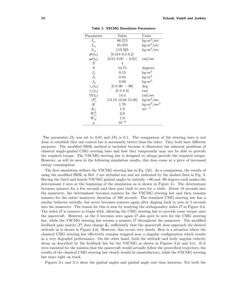
A rigid spacecraft with some initial body angular velocity ω and non-zero attitude σ is to bebrought to rest at a zero attitude vector. The σ vector is assumed to be measured from a desiredattitude. Four equal VSCMGs are embedded in the spacecraft in a standard pyramid configurationas shown in Figure 2. All simulation parameters are shown in Table 1. The angular velocity feedbackmatrix [P ] is chosen to be of diagonal form with the entries shown in the table. The initial γ valueis only used in the gimbal acceleration based steering law.

The VSCMG steering laws are compared to the single-gimbal CMG steering laws presented by Ohand Vadali in Ref. 1. Their steering law combines the Singularity Robustness Steering Law (SRSL)

γ = [D1]T([D1][D1]T + αI3x3

)−1Lr (77)

with a variable angular velocity feedback gain matrix [P ]. The parameter α depends on the singu-larity index δ through

α = α0e−δ (78)

The SRSL smoothly handles rank deficient [D1] matrices by having a slightly inaccurate matrixinverse. To escape situations where the orthogonality index O has gone to zero, the required torqueis varied by changing the feedback gain matrix [P ] elements through

[P ] =

P1 −δP δPδP P2 −δP−δP δP P3

(79)

where the smoothly varying parameter δP is related to the orthogonality factor through

δP =

δP0

O0−OO0

for O < O0

0 for O ≥ O0

(80)


Table 1: VSCMG Simulation Parameters

Parameter Value UnitsIs1 86.215 kg-m2/secIs2 85.070 kg-m2/secIs3 113.565 kg-m2/sec

σ(t0) [0.414 0.3 0.2]ω(t0) [0.01 0.05 − 0.01] rad/sec

N 4θ 54.75 degreesJs 0.13 kg-m2

Jt 0.04 kg-m2

Jg 0.03 kg-m2

γi(t0) [0 0 90 − 90] degγi(t0) [0 0 0 0] radΩ(t0) 14.4 rad/sec[P ] [13.13 13.04 15.08] kg-m2/secK 1.70 kg-m2/sec2

Kγ 1.0 sec−1

W 0si

2.0Wgi 1.0µ 10−9

The parameter O0 was set to 0.01 and δP0 is 0.1. The comparison of the steering laws is notdone to establish that one control law is necessarily better than the other. They both have differentpurposes. The modified SRSL method is included because it illustrates the inherent problems ofclassical single-gimbal CMG steering laws and how they temporarily may not be able to providethe required torque. The VSCMG steering law is designed to always provide the required torque.However, as will be seen in the following simulation results, this does come at a price of increasedenergy consumption.

The first simulation utilizes the VSCMG steering law in Eq. (56). As a comparison, the results ofusing the modified SRSL in Ref. 1 are included too and are indicated by the dashed lines in Fig. 3.Having the third and fourth VSCMG gimbal angles be initially +90 and -90 degrees each makes thedeterminant δ zero at the beginning of the simulation as is shown in Figure 3.i. The determinantbecomes nonzero for a few seconds and then goes back to zero for a while. About 18 seconds intothe maneuver, the determinant becomes nonzero for the VSCMG steering law and then remainsnonzero for the entire maneuver duration of 500 seconds. The standard CMG steering law has asimilar behavior initially, but never becomes nonzero again after dipping back to zero at 5 secondsinto the maneuver. The reason for this is seen by studying the orthogonality index O in Figure 3.ii.The index O is nonzero to begin with, allowing the CMG steering law to provide some torque ontothe spacecraft. However, as the δ becomes zero again O also goes to zero for the CMG steeringlaw, while the VSCMG steering law retains a nonzero O throughout the maneuver. The modifiedfeedback gain matrix [P ] does change Lr sufficiently that the spacecraft does approach the desiredattitude as is shown in Figure 3.iii. However, this occurs very slowly. Here is a situation where theclassical CMG steering law effectively remains trapped near a singular configuration which resultsin a very degraded performance. On the other hand, both the attitude and body angular velocitydecay as described by the feedback law for the VSCMG as shown in Figures 3.iii and 3.iv. If itwere essential for the mission that the spacecraft would actually follow the prescribed trajectory, theresults of the classical CMG steering law clearly would be unsatisfactory, while the VSCMG steeringlaw stays right on track.

Figures 3.v and 3.vi show the gimbal angles and gimbal angle rate time histories. For both the


0 10 20 30 40

0

20

40

60

80

VSCMG

CMGD

eter

min

ant

δ

(i) Determinant δ

0 10 20 30 4002468

1012141618

VSCMG

CMG

Ort

hogo

nalit

y M

easu

re O

(ii) Orthogonality Index O

0 100 200 300 400 500

0.00

0.10

0.20

0.30

0.40 VSCMG

CMG

Atti

tude

Vec

tor

σ

(iii) MRP Attitude Vector

0 50 100 150 200-0.05-0.04-0.03-0.02-0.010.000.010.020.030.040.05

VSCMG

CMG

Ang

. Vel

. Vec

tor

[rad

/s]

ω(iv) Body Ang. Vel. Vector

γ

0 50 100 150 200-300-250-200-150-100

-500

50100150

VSCMG

CMG

Gim

bal A

ngle

[de

g]

(v) Gimbal Angles

0 10 20-1.0-0.8-0.6-0.4-0.20.00.20.40.60.81.0

VSCMG

CMG

Gim

bal A

ngle

Rat

es

[

rad/

s]γ

(vi) Gimbal Angle Rates

0 50 100 150-0.2

0.0

0.2

0.4

0.6

0.8

1.0

1.2

time [s]

Required Torque

Actual Torque

Stee

ring

Tor

que

[N

-m]

(vii) Required vs. Actual Steering Torque

0 10 2010121416182022242628

time [s]

RW

Spi

n Sp

eed

[rad

/s]

Ω

(viii) RW spin speed

Figure 3: Gimbal Velocity Based Steering Law Simulation


VSCMG and CMG steering law the gimbal rates are relatively large at the beginning of the maneuverwhere the CMGs remain close to a singular configuration. After about 6 seconds the CMG ratesremain almost zero because the steering law is essentially “entrapped” in the singular configuration.Figure 3.vii compares the required torque Lr to the actual torque La produced by the CMG steeringlaw. The VSCMG actual torque is not shown in this figure because it is always equal to Lr. Whilehaving the SRSL and the time varying [P ] matrix to help the standard CMG steering law and thisspacecraft would eventually reach the desired target state, this Figure shows clearly that the actualtorque produced at several time segments much less than the required torque. However, for theVSCMG steering law to keep the spacecraft on track comes at the expense of spinning the RW upor down on occasion. The RW spin speeds Ω are shown in Figure 3.viii. The RW mode is employedtwice when the determinant δ goes to zero. Once the CMGs are away for a singular configuration,the spin speeds remain essentially constant.

0 5 10 15 20-1.0-0.8-0.6-0.4-0.20.00.20.40.60.8

Acc. Steering Law

Vel. Steering Law

Gim

bal A

ngle

Rat

e

[r

ad/s

]γ

(i) Gimbal Ang. Rates

γG

imba

l Ang

le R

ate

[

rad/

s]50 100 150 200

-0.02

-0.01

0.00

0.01

0.02 Acc. Steering Law

Vel. Steering Law

(ii) Gimbal Ang. Rates

0 100 200 300 400 500-200

-150

-100

-50

0

50

100

150

time [s]

Acc. Case

Vel. Case

Gim

bal A

ngle

[de

g]γ

(iii) Gimbal Angles

0 100 200 300 400 50010-710-610-510-410-310-210-1100101

time [s]

VSCMG

CMG

Wor

k R

ate

[J/

s]

(iv) Work Rates

Figure 4: Gimbal Acceleration Based Steering Law Simulation

The second simulation uses the gimbal acceleration based steering law in Eq. (68) and the resultsare shown in Figure 4. The gimbal acceleration were designed such that they would provide thesame performance as the velocity based steering law. Figures 4.i and 4.ii show the gimbal anglerates for both the gimbal acceleration and velocity based steering laws. As expected, during theinitial phase of the maneuver the two gimbal rates are quite different as seen in Figure 4.i. This isbecause the initial gimbal rates were set to zero and were not equal to the desired gimbal rates fromEq. (56). However, as Figure 4.ii shows clearly, after about 10 to 20 seconds into the maneuver, thegimbal rate performance of the acceleration steering approaches that of the desired velocity basedsteering law. The corresponding gimbal angles for both cases are shown in Figure 4.iii.

The natural drawback to using the RW modes of the VSCMG to maneuver through classical CMGsingularities is evident when studying the work rate of the VSCMG steering law compared to the


standard CMG steering law in Figure 4.iv. The work rate W for the VSCMGs is defined as

W =N∑

i=1

|Ωiusi |+ |γiugi | (81)

During the initial phase of the maneuver, where the determinant δ is very small, the energy con-sumption to drive the RW modes is relatively large compared to the CMG modes. Away from thissingularity, the energy consumption is very comparable to that of the CMG steering law. The powerof RW torques is typically the limiting factor for the VSCMG devices to decide on how large a struc-ture they could be used. However, for smaller spacecraft which may be able to afford temporaryRW modes, the VSCMG steering law provides interesting possibilities. Other authors have lookedinto augmenting CMG cluster with thrusters to keep the spacecraft on track during near singularconfigurations. Using the RW modes has several benefits over using thrusters. They provide a muchsmoother response compared to using thrusters and will excite few flexible modes within the space-craft. Also, RW don’t require propellant to operate, but use electrical power which can be readilyrecharged from solar arrays.

0 20 40 60 80 100-50-40-30-20-10

0102030405060

time [s]

Gim

bal A

ngle

s [

deg]

(i) Gimbal Angles γ

0 20 40 60 80 100-0.10-0.08-0.06-0.04-0.020.000.020.040.060.080.100.12

time [s]

Gim

bal R

ate

[ra

d/s]

(ii) Gimbal Ang. Rates γ

0 20 40 60 80 10013.413.613.814.014.214.414.614.815.015.215.4

time [s]

RW

Ang

. Vel

ocity

[ra

d/s]

(iii) RW Spin Speeds Ω

0 20 40 60 80 100-0.003

-0.002

-0.001

0.000

0.001

0.002

0.003

time [s]

RW

Mot

or T

orqu

e [N

-m]

(iv) RW Motor Torques us

Figure 5: Reconfiguring the CMG Gimbals using VSCMG Null Motion

The third simulation shown in Figure 5 illustrates the use of the VSCMG null motion to reorientthe CMGs to a set of preferred gimbal angles where the final Ω was irrelevant (i.e. aRW = 1 andaCMG = 1). The initial and preferred gimbal angles are (0, 0, 0, 20) degrees and (45, 45,−45,−45)degrees respectively. The scalar ke was set to 0.1 and the weights Wsi

were held constant at 2. Notethat this gimbal angle reconfiguration cannot be performed with the classical CMG null motionwhere Ω is held constant, because the initial configuration has an internal momentum vector andthe preferred configuration would have none. The performance of the classical CMG null motion is


shown in Figure 5 through dashed lines. Figure 5.i clearly shows that the VSCMG null motion is ableto reconfigure the γ much closer to γf than the CMG null motion. The corresponding gimbal ratesγ, shown in Figure 5.ii, are smooth and remain relatively small compared to the maximum allowablegimbal rates of 2 rad/s. The VSCMGs achieve this feat by varying the RW spin speeds. However,as shown in Figure 5.iii, they do not have to be changed much to prevent a torque being appliedonto the spacecraft. The corresponding torque required by the RW motors is shown in Figure 5.iv.The magnitude of these torques are of the same order as the RW torques required by the classicalCMG to maintain a constant Ω during a spacecraft reorientation. Therefore, no hardware changewould be required to use the VSCMG null motion to reconfigure the gimbal angles, only a changein the feedback control law of the RW speeds.

Another simulation was performed where the initial gimbal angles were (0, 0, 0, 0) degrees as wasdone in Ref. 23. Note that this reconfiguration can be accomplished with CMG null motion becausethe initial and final configuration has the same internal momentum vector. The VSCMG null motionwas identical to the CMG null motion where Ω was held constant even though Wsi was held constantat 2. The minimum norm inverse automatically used the more efficient CMG mode here.

Besides reorienting the gimbals with the VSCMG null motion, it is also possible to change the RWspin speeds Ω to desired values by setting aRW = 1. The extra degrees of control allow the internalmomentum vector to be redistributed across the CMG and RW modes in an infinity of ways. Alimiting factor in how fast this reconfiguring can be done is the typically the maximum allowableRW motor torques. The speed of the VSCMG null motion is directly control by the size of ke.

Conclusions

The equations of motion of a rigid spacecraft with N VSCMGs embedded are introduced, includingthe physical control torques required by the gimbal and the RW motors. A globally asymptoticallystable feedback control law based on Lyapunov theory is developed to stabilize the spacecraft at agiven attitude. The velocity based steering law contains a weighted minimum norm inverse. TheRW mode weights depend on the proximity of the gimbal frame to a classical single-gimbal CMGsingularity. Away from such a singularity the RW mode weights are essentially zero and the VSCMGperforms like a CMG. Close to a singularity the CMG mode is augmented with the RW mode toensure that the required torque Lr is always precisely produced. An acceleration based steering lawis also presented that will yield the desired velocity based steering law performance and allows forwork rate studies. Further, the use of the VSCMG null motion to reconfigure the gimbal angles andRW speeds is presented. The gimbal angles are able to be reoriented in a much more general mannerthan was possible with the CMG null motion, thus making it easier to avoid singularities altogether.The resulting torques required of the RW motors are typically well within the current capabilitiesof single-gimbal CMG reaction wheel motors. Therefore, utilizing the VSCMG null motion in thismanner would only require a change the RW feedback law and not necessary a hardware redesign.

References

[1] H. S. Oh and S. R. Vadali. “Feedback Control and Steering Laws for Spacecraft Using Single GimbalControl Moment Gyros,” Journal of the Astronautical Sciences, Vol. 39, No. 2, April–June 1991, pp.183–203.

[2] B. R. Hoelscher and S. R. Vadali. “Optimal Open-Loop and Feedback Control Using Single GimbalControl Moment Gyroscopes,” Journal of the Astronautical Sciences, Vol. 42, No. 2, April–June 1994,pp. 189–206.

[3] S. Krishnan and S. R. Vadali. “An Inverse-Free Technique for Attitude Control of Spacecraft UsingCMGs,” Acta Astronautica, Vol. 39, No. 6, 1997, pp. 431–438.

[4] N. S. Bedrossian. Steering Law Design for Redundant Single Gimbal Control Moment Gyro Systems.M.S. Thesis, Mechanical Engineering, MIT, Aug. 1987.

[5] J. L. Junkins and J. D. Turner. Optimal Spacecraft Rotational Maneuvers. Elsevier Science Publishers,Amsterdam, Netherlands, 1986.


[6] H. Schaub, R. D. Robinett, and J. L. Junkins. “Globally Stable Feedback Laws for Near-Minimum-Fueland Near-Minimum-Time Pointing Maneuvers for a Landmark-Tracking Spacecraft,” Journal of theAstronautical Sciences, Vol. 44, No. 4, Oct.–Dec. 1996, pp. 443–466.

[7] K. Ford and C. D. Hall. “Flexible Spacecraft Reorientations Using Gimbaled Momentum Wheels,”AAS/AIAA Astrodynamics Specialist Conference, Sun Valley, Idaho, August 1997. Paper No. 97-723.

[8] D. T. Greenwood. Principles of Dynamics. Prentice-Hall, Inc, Englewood Cliffs, New Jersey, 2ndedition, 1988.

[9] W. E. Wiesel. Spaceflight Dynamics. McGraw-Hill, Inc., New York, 1989.

[10] H. S. Oh, S. R. Vadali, and J. L. Junkins. “On the Use of the Work-Energy Rate Principle for DesigningFeedback Control Laws,” AIAA Journal of Guidance, Control and Dynamics, Vol. 15 No. 1, Jan–Feb1992, pp. 272–277.

[11] H. Schaub and J. L. Junkins. “Stereographic Orientation Parameters for Attitude Dynamics: A Gener-alization of the Rodrigues Parameters,” Journal of the Astronautical Sciences, Vol. 44, No. 1, Jan.–Mar.1996, pp. 1–19.

[12] P. Tsiotras, J. L. Junkins, and H. Schaub. “Higher Order Cayley Transforms with Applications toAttitude Representations,” Journal of Guidance, Control and Dynamics, Vol. 20, No. 3, May–June1997, pp. 528–534.

[13] P. Tsiotras. “Stabilization and Optimality Results for the Attitude Control Problem,” Journal ofGuidance, Control and Dynamics, Vol. 19, No. 4, 1996, pp. 772–779.

[14] T. F. Wiener. Theoretical Analysis of Gimballess Inertial Reference Equipment Using Delta-ModulatedInstruments. Ph.D. dissertation, Department of Aeronautics and Astronautics, Massachusetts Instituteof Technology, March 1962.

[15] S. R. Marandi and V. J. Modi. “A Preferred Coordinate System and the Associated OrientationRepresentation in Attitude Dynamics,” Acta Astronautica, Vol. 15, No. 11, 1987, pp. 833–843.

[16] M. D. Shuster. “A Survey of Attitude Representations,” Journal of the Astronautical Sciences, Vol. 41,No. 4, 1993, pp. 439–517.

[17] H. Schaub, P. Tsiotras, and J. L. Junkins. “Principal Rotation Representations of Proper NxN Orthog-onal Matrices,” International Journal of Engineering Science, Vol. 33, No. 15, 1995, pp. 2277–2295.

[18] J. L. Junkins and Y. Kim. Introduction to Dynamics and Control of Flexible Structures. AIAA EducationSeries, Washington D.C., 1993.

[19] R. Mukherjee and D. Chen. “Asymptotic Stability Theorem for Autonomous Systems,” Journal ofGuidance, Control, and Dynamics, Vol. 16, Sept.–Oct. 1993, pp. 961–963.

[20] R. Mukherjee and J. L. Junkins. “Invariant Set Analysis of the Hub-Appendage Problem,” Journal ofGuidance, Control, and Dynamics, Vol. 16, Nov.–Dec. 1993, pp. 1191–1193.

[21] J. L. Junkins. An Introduction to Optimal Estimation of Dynamical Systems. Sijthoff & NoordhoffInternational Publishers, Alphen aan den Rijn, Netherlands, 1978.

[22] Y. Nakamura and H. Hanafusa. “Inverse Kinematic Solutions with Singularity Robustness for RobotManipulator Control,” Journal of Dynamic Systems, Measurement, and Control, Vol. 108, Sept. 1986,pp. 164–171.

[23] S. R. Vadali, H. S. Oh, and S. R. Walker. “Preferred Gimbal Angles for Single-Gimbal Control MomentGyros,” Journal of Guidance, Control and Dynamics, Vol. 13, No. 6, Nov.–Dec. 1990, pp. 1090–1095.

Feedback Control Law for Variable Speed Control Moment...

Documents

Transcript of Feedback Control Law for Variable Speed Control Moment...