arX

iv:1

211.

4952

v2 [

quan

t-ph

] 1

5 N

ov 2

013

A discussion on the origin of quantum probabilities

Federico Holik1,2 , Angel Plastino3 and Manuel Saenz2

October 18, 2018

1- Universidad Nacional de La Plata, Instituto de Fısica (IFLP-CCT-CONICET), C.C. 727, 1900 LaPlata, Argentina

2- Departamento de Matematica - Facultad de Ciencias Exactas y NaturalesUniversidad de Buenos Aires - Pabellon I, Ciudad Universitaria

Buenos Aires, Argentina.3- Universitat de les Illes Balears and IFISC-CSIC, 07122 Palma de Mallorca, Spain

Abstract

We study the origin of quantum probabilities as arising from non-boolean propositional-operational structures. We apply the method developed by Cox to non distributive latticesand develop an alternative formulation of non-Kolmogorvian probability measures for quan-tum mechanics. By generalizing the method presented in previous works, we outline a generalframework for the deduction of probabilities in general propositional structures representedby lattices (including the non-distributive case).

Key words: Quantum Probability-Lattice theory-Information theory

1 Introduction

Quantum probabilities1 posed an intriguing question from the very beginning of quantum theory.It was rapidly realized that probability amplitudes of quantum process obeyed rules of a nonclassical nature, as for example, the sum rule of probability amplitudes giving rise to interferenceterms or the nonexistence of joint distributions for noncommuting observables. In 1936 vonNeumann wrote the first work ever to introduce quantum logics [1, 2, 3], suggesting that quantummechanics requires a propositional calculus substantially different from all classical logics. Herigorously isolated a new algebraic structure for quantum logics, and studied its connections withquantum probabilities. Quantum and classical probabilities have points in common as well asdifferences. These differences and the properties of quantum probabilities have been intensivelystudied in the literature [4, 5, 6, 7, 8, 9, 10, 11, 12, 13, 14]. It is important to remark that notall authors believe that quantum probabilities are essentially of a different nature than thosewhich arise in probability theory (see for example [26] for a recent account). Thought this is a

1By the term “quantum probabilities”, we mean the probabilities that appear in quantum theory. As is wellknown, they are ruled by the well known formula tr(ρP ), where ρ is a density matrix representing a generalquantum state and P is a projection operator representing an event (see Section 4 of this work for details).

1

major question for probability theory and physics, it is not our aim in this work to settle thisdiscussion.There exist two important axiomatizations of classical probabilities. One of them was providedby Kolmogorov [15], a set theoretical approach based on boolean sigma algebras of a samplespace. Probabilities are defined as measures over subsets of a given set. Thus, the Kolmogoro-vian approach is set theoretical and usually identified (but not necessarily) with a frequentisticinterpretation of probabilities. Some time later it was realized that quantum probabilities can beformulated as measures over non boolean structures (instead of boolean sigma algebras). Thisis the origin of the name “non-boolean or non-kolmogorovian” probabilities [8]. It is remark-able that the creation of quantum theory and the works on the foundations of probability byKolmogorov where both developed at the same time, in the twenties.An alternative approach to the Kolmogorovian construction of probabilities was developed byR. T. Cox [16, 17]. Cox starts with a propositional calculus, intended to represent assertionswhich portray our knowledge about the world or system under investigation. As it is well knownsince the work of Boole [18], propositions of classical logic (CL) can be represented as a Booleanlattice, i.e., an algebraic structure endowed with lattice operations “∧”, “∨”, and “¬”, whichare intended to represent conjunction, disjunction, and negation, respectively, together with apartial order relation “≤” which is intended to represent logical implication. Boolean lattices(as seen from an algebraic point of view) can be characterized by axioms [19, 20, 21]. Byconsidering probabilities as an inferential calculus on a boolean lattice, Cox showed that theaxioms of classical probability can be deduced as a consequence of lattice symmetries, usingentropy as a measure of information. Thus, differently form the set theoretical approach ofKolmogorov, the approach by Cox considers probabilities as an inferential calculus.

It was recently shown that Feymann’s rules of quantum mechanics can be deduced from oper-ational lattice structures using a variant of Cox method [24, 25, 26, 27, 28] (see also [19, 20]).For example, in [26, 27] this is done by:

• first defining an operational propositional calculus on a quantum system under study, andafter that,

• postulating that any quantum process (interpreted as a proposition in the operationalpropositional calculus) can be represented by a pair of real numbers and,

• using a variant of the method developed by Cox, showing that these pairs of real numbersobey the sum and product rules of complex numbers, and can then be interpreted as thequantum probability amplitudes which appear in Feymann’s rules.

There is a long tradition with regards to the application of lattice theory to physics and manyother disciplines. The quantum logical (QL) approach to quantum theory (and physics in gen-eral), initiated by von Neumann in [1], has been a traditional tool for studies on the foundationsof quantum mechanics (see for example [29, 30, 31, 32, 33, 34, 35, 36, 37, 38, 39, 5], and for acomplete bibliography [6], [40], and [41]).The (QL) approach to physics bases itself on defining elementary tests and propositions forphysical systems and then, studying the nature of these propositional structures. In someapproaches, this is done in an operational way [31, 42, 43, 44, 45, 46], and is susceptible ofconsiderable generalization to arbitrary physical systems (not necessarily quantum ones). Thatis why the approach is also called operational quantum logic (OQL)2. One of the most importantgoals of OQL is to impose operationally motivated axioms on a lattice structure in order that it

2In this paper we will use the terms QL and OQL interchangeably, but it is important to remark that -thoughsimilar- they are different approaches.

2

can be made isomorphic to a projection lattice on a Hilbert space. There are different positionsin the literature about the question of whether this goal has been achieved or not [14], andalso, of course, alternative operational approaches to physics, as the convex operational one[47, 48, 49, 50, 51, 4]. In this work, we are interested in the great generality of the OQLapproach. The operational approach presented in [4] bases itself only in the convex formulationof any statistical theory, and it can be shown that the more general structure which appearsunder reasonable operational considerations is a σ-orthocomplemented orthomodular poset, amore general class than orthomodular lattices (the ones which appear in quantum theory). Wewill come back to these issues and review the definitions for these structures below.In this work we complement the work presented in [20, 21] asking the following questions:

• is it possible to generalize Cox’s method to arbitrary lattices or more general algebraicstructures?

• what happens if the Cox’s method mentioned above is applied to general lattices (notnecessarily distributive), representing general physical systems? And in particular, whathappens if it is applied to the von Newmann’s lattice of projection operators?

• does the logical underlying structure of the theory determine the form and propertiesof the probabilities?

As we shall see below, it is possible to use these questions to give an alternative formulationof quantum probabilities. We will show that once the operational structure of the theoryis fixed, the general properties of probability theory are -in a certain sense to be clarifiedbelow- determined. We also discuss the implications of our derivation for the foundations ofquantum physics and probability theory, and compare with ours different approaches: the onepresented in [26, 27], the OQL approach, the operational approach of [4], and the traditionalone (represented by the von Neumann formalism of Hilbertian quantum mechanics [52]).The approach presented here shows itself to be susceptible of great generalization: we providean algorithm for developing generalized probabilities using a combination of the Cox’s methodwith the OQL approach. This opens the door to the development of more general probabilityand information measures. This methodology is advantageous because, in the particular caseof quantum mechanics, it includes mixed states in a natural way, unlike other approachesbased only on pure states (like the ones presented in [28] and [24]).

The paper is organized as follows. In Section 2 we review the QL approach to physics as well aslattice theory. In Section 3 we revisit Kolmogorov’s and Cox’ approaches to probability. Afterthat, in Section 4, we give a sketch concerning quantum probabilities and their differences withclassical ones. In Section 5 we discuss the approach developed in [24], [25], [26], [27], and [28]. InSection 6 we apply Cox’s method for the formulation of non-Kolmogorovian probabilities usingthe algebraic properties of non-boolean lattices and study several examples. Finally, in section7 some conclusions are drawn.

2 The lattice/operational approach to physics

The quantum logical approach to physics is vast and includes different programs. We willconcentrate on the path followed by von Neumann and the operational approach developed byJauch, Piron, and others. First, we recall the relationship between projection operators andelementary tests in QM . After studying the examples of lattices applied to QM and CM, wereview the main features of the QL approach. The reader familiar with these topics can skipthis Section.

3

2.1 Elementary notions of lattice theory

A partially ordered set (also called a poset) is a set X endowed with a partial ordering relation“<” satisfying

• 1- For all x, y ∈ X, x < y and y < x entail x = y

• 2- For all x, y, z ∈ X, if x < y and y < z, then x < z

The notation “x ≤ y” is used to denote “x < y” or “x = y”. A lattice L will be a poset in whichany two elements a and b have a unique supremum (the elements’ least upper bound “a ∨ b”;called their join) and an infimum (greatest lower bound “a∧ b”; called their meet). Lattices canalso be characterized as algebraic structures satisfying certain axiomatic identities imposed onoperations “∨” and “∧”. For a complete lattice all its subsets have both a supremum (join) andan infimum (meet).

A bounded lattice has a greatest (or maximum) and least (or minimum) element, denoted 1 and0 by convention (also called top and bottom, respectively). Any lattice can be converted intoa bounded lattice by adding a greatest and least element, and every non-empty finite latticeis bounded. For any set A, the collection of all subsets of A (called the power set of A) canbe ordered via subset inclusion to obtain a lattice bounded by A itself and the null set. Setintersection and union represent the operations meet and join, respectively.

Every complete lattice is a bounded lattice. While bounded lattice homomorphisms in generalpreserve only finite joins and meets, complete lattice homomorphisms are required to preservearbitrary joins and meets. If P is a bounded poset, an orthocomplementation in P a unaryoperation “¬(. . .)” such that:

¬(¬(a))) = a (1a)

a ≤ b −→ ¬b ≤ ¬a (1b)

a ∨ ¬a and a ∧ ¬a exist and botha ∨ ¬a = 1 (1c)

a ∧ ¬a = 0 (1d)

hold. A bounded poset with ortocomplementation will be called an orthoposet. An ortholattice,will be an orthoposet which is also a lattice. For a, b ∈ L (an ortholattice or orthoposet), wesay that a is orthogonal to b (a⊥b) iff a ≤ ¬b.

Distributive lattices are lattices for which the operations of join and meet are distributed overeach other. A complete complemented lattice that is also distributive is a Boolean algebra. Fora distributive lattice, the complement of x, when it exists, is unique. The prototypical examplesof Boolean algebras are collections of sets for which the lattice operations can be given by setunion and intersection, and lattice complementation by set theoretical complementation.A modular lattice is one that satisfies the following self-dual condition (modular law or modularidentity)

x ≤ b −→ x ∨ (a ∧ b) = (x ∨ a) ∧ b (2)

Modular lattices arise naturally in algebra and in many other areas of mathematics. For example,the subspaces of a finite dimensional vector space form a modular lattice. Every distributivelattice is modular. In a not necessarily modular lattice, there may still be elements b for which

4

the modular law holds in connection with arbitrary elements a and x (≤ b). Such an elementis called a modular element. Even more generally, the modular law may hold for a fixed pair(a, b). Such a pair is called a modular pair, and there are various generalizations of modularityrelated to this notion and to semi-modularity.

An orthomodular lattice will be an ortholattice satisfying the orthomodular law:

x ≤ b −→ x ∨ (¬x ∧ b) = b (3)

Orthomodularity is a weakening of modularity. As an example, the lattice LvN (H) of closedsubspaces of a Hilbert space H (see Section 2.2) is orthomodular. LvN (H) is modular only if His finite dimensional and strictly orthomodular for the infinite dimensional case.

The concept of lattice’s atom is of great physical importance. If L has a least element 0, thenan element x of L is an atom if 0 < x and there exists no element y of L such that 0 < y < x.One says that L is:i) Atomic, if for every nonzero element x of L, there exists an atom a of L such that a ≤ xii) Atomistic, if every element of L is a supremum of atoms.

2.2 Elementary measurements and projection operators

In QM, an elementary measurement given by a yes-no experiment (i.e., a test in which we getthe answer “yes” or the answer “no”), is represented by a projection operator. If R is the realline, let B(R) be the family of subsets of R such that

• 1 - The family is closed under set theoretical complements.

• 2 - The family is closed under denumerable unions.

• 3 - The family includes all open intervals.

The elements of B(R) are the Borel subsets of R [53]. Let P(H) be the set of all projectionoperators (or equivalently, the set of closed subspaces of H). In QM, a projection valued measure(PVM) M , is a mapping

M : B(R) → P(H) (4a)

such that

M(∅) = 0 (4b)

M(R) = 1 (4c)

M(∪j(Bj)) =∑

j

M(Bj), (4d)

for any disjoint denumerable family Bj . Also,

M(Bc) = 1−M(B) = (M(B))⊥ (4e)

Any elementary measurement is represented by a projection operator [52]. All operators repre-senting observables can be expressed in terms of PVM’s (and so, reduced to sets of elementarymeasurements), via the spectral decomposition theorem, which asserts that the set of spectral

5

measurements may be put in a bijective correspondence with the set A of self adjoint operatorsof H [53].

The set of closed subspaces P(H) of any quantum system can be endowed with a lattice structure:LvN (H) =< P(H), ≤, ∧, ∨, ¬, 0, 1 >, where “≤” is the set theoretical inclusion “⊆”, “∧”is set theoretical intersection “∩”, “∨” is the closure of the sum“⊕”, 0 is the empty set ∅, 1 isthe total space H and ¬(S) is the orthogonal complement of a subspace S [7]. Closed subspacescan be put in one to one correspondence with projection operators. Thus, elementary tests inQM, which are represented by projection operators, can be endowed with a lattice structure. Thislattice was called “Quantum Logic” by Birkhoff and von Neumann [1]. We will refer to thislattice as the von Neumann-lattice (LvN (H)) [7].

The analogous of this structure in Classical Mechanics (CM) was provided by Birkoff and vonNeumann [1]. Take for example the following operational propositions on a classical harmonicoscillator: “the energy is equal to E0” and “the energy is lesser or equal than E0”. The firstone corresponds to an ellipse in phase space, and the second to the ellipse and its interior. Thissimple example shows that operational propositions in CM can be represented by subsets of thephase space. Thus, given a classical system S with phase space Γ, let P(Γ) represent the setformed by all the subsets of Γ. This set can be endowed with a lattice structure as follows. If“∨” is represented by set union, “∧” by set intersection, “¬” by set complement (with respectto Γ), ≤ is represented by set inclusion, and 0 and 1 are represented by ∅ and Γ respectively,then < P(Γ), ≤, ∧, ∨, ¬, 0, 1 > conform a complete bounded lattice. This is the lattice ofpropositions of a classical system, which as it is well known, is a boolean one. Thus, P(Γ), aswell as P(H), can be endowed with a propositional lattice structure.

2.3 The Quantum Logical Approach to Physics

We have seen that operational propositions of quantum and classical systems can be endowedwith lattice structures. These lattices where boolean for classical systems, and non distributivefor quantum ones. This fact, discovered by von Neumann [1], raised a lot of interesting questions.The first one is: is it possible to obtain the formalism of QM (as well as CM) by imposingsuitable axioms on a lattice structure? The surprising answer is yes, it is possible. But theroad which led to this result was fairly difficult and full of obstacles. In the first place, it was avery difficult mathematical task to demonstrate that a suitably chosen set of axioms on a latticewould yield a representation theorem which would allow one to recover Hilbertian QM . The firstresult was obtained by Piron, and the final demonstration was given by Soler in 1995 [54] (seealso [6], page 72). One of the advantages ascribed to this approach was that the axioms imposedon a lattice structure could be given a clear operational interpretation: unlike the Hilbert spaceformulation, whose axioms have the disadvantage of being ad hoc and physically unmotivated,the quantum logical approach would be clearer and more intuitive from a physical point ofview. But of course, the operational validity of the axioms imposed on the lattice structure wascriticized by many authors (as an example, see [14]).

The second important question raised by the von Neumann discovery was: given that QM andCM can be described by operational lattices, is it possible to formulate the entire apparatus ofphysics in lattice theoretical terms? Given any physical system, quantum, classical, or obeyingmore general tenets, it is always possible to define an operational propositional structure on itusing the notion of elementary tests. A very general approach to physics can be given usingevent structures, which are sets of events endowed with probability measures satisfying certainaxioms [4]. It can be shown (see [4], Chapter 3) that any event structure is isomorphic toa σ-orthocomplete orthomodular poset, which is an orthocomplemented poset P, satisfying the

6

orthomodular identity (3), and for which if ai ∈ P and ai⊥aj (i 6= j), this implies that∨

ai existsfor i = 1, 2, . . .. Remark that event structures (or σ-orthocomplete orthomodular posets) neednot to be lattices. However, lattices are very general structures and encompass most importantexamples. Consequently, we will work with orthomodular lattices in this paper (and indicatewhich results can be easily extended to σ-orthocomplete orthomodular posets).There are other general approaches to statistical theories. One of them is the convex operationalone [55, 56, 57, 58], which consists on imposing axioms on a convex structure (formed by physicalstates). Indeed, the convex operational approach is even more general than the quantum logical,but we will not discuss this issue in detail here (although a link with it will be discussed in Section6.5).

3 Cox vs. Kolmogorov

In this Section we will review two different approaches to probability theory. On one hand, theCox’s approach, in which probabilities are considered as measures of the plausibility of a givenevent or happening. On the other hand, the traditional Kolmogorovian one, a set theoreticalapproach which is compatible with the interpretation of probabilities as frequencies.

3.1 Kolmogorov

Given a set Ω, let us consider a σ-algebra Σ of Ω. Then, a probability measure will be given bya function µ such that

µ : Σ → [0, 1] (5a)

which satisfiesµ(∅) = 0 (5b)

µ(Ac) = 1− µ(A), (5c)

where (. . .)c means set-theoretical-complement and for any pairwise disjoint denumerable familyAii∈I

µ(⋃

i∈I

Ai) =∑

i

µ(Ai) (5d)

where conditions (5) are the well known axioms of Kolmogorov. The triad (Ω,Σ, µ) is calleda probability space. Depending on the context, probability spaces obeying Eqs. (5) are usuallyreferred as Kolmogorovian, classical, commutative or boolean probabilities [4].It is possible to show that if (Ω,Σ, µ) is a kolmogorovian probability space, the inclusion-exclusion principle holds

µ(A ∪B) = µ(A) + µ(B)− µ(A ∩B) (6)

or (as expressed in logical terms)

µ(A ∨B) = µ(A) + µ(B)− µ(A ∧B) (7)

As remarked in [59], Eq. (6) was considered as crucial by von Neumann for the interpretation ofµ(A) and µ(B) as relative frequencies. If N(A∪B), N(A), N(B), N(A∩B) are the number of timesof each event to occur in a series of N repetitions, then (6) trivially holds.

7

As we shall discuss below, this principle does no longer hold in QM, a fact linked to the non-boolean QM-character. Thus, the relative-frequencies’ interpretation of quantum probabilitiesbecomes problematic [59]. The QM example shows that non-distributive propositional structuresplay an important role in probability theories different from that of Kolmogorov.

3.2 Cox’s approach

Propositions of classical logic can be endowed with a Boolean lattice structure [18]. The logicalimplication “−→” is associated with a partial order relation “≤”, the conjunction “and” withthe greatest lower bound “∧”, disjunction “or” with the lowest upper bound “∨”, and negation“not” is associated with complement “¬”. Boolean lattices can be characterized as ortholatticessatisfying:

• L1. x ∨ x = x, x ∧ x = x (idempotence)

• L2. x ∨ y = y ∨ x, x ∧ y = y ∧ x (commutativity)

• L3. x ∨ (y ∨ z) = (x ∨ y) ∨ z, x ∧ (y ∧ z) = (x ∧ y) ∧ z (associativity)

• L4. x ∨ (x ∧ y) = x ∧ (x ∨ y) = x (absortion)

• D1. x ∧ (y ∨ z) = (x ∧ y) ∨ (x ∧ z) (distributivity 1)

• D2. x ∨ (y ∧ z) = (x ∨ y) ∧ (x ∨ z) (distributivity 2)

It is well known that boolean lattices can be represented as subsets of a given set, with “≤”represented as set theoretical inclusion ⊆, “∨” represented as set theoretical union “∪”, “∧”represented as set intersection “∩”, and ¬ represented as the set theoretical complement “(. . .)c”.

As a typical feature, Cox develops classical probability theory as an inferential calculus onboolean lattices. A real valued function ϕ representing the degree to which a proposition yimplies another proposition x is postulated, and its properties deduced from the algebraic prop-erties of the boolean lattice (Eqns. (1) and (3.2)). These algebraic properties define functionalequations [60] which determine the possible elections of ϕ up to rescaling. It turns out thatϕ(x|y) –if suitably normalized– satisfies all the properties of a Kolmogorovian probability (Eqs.(5)). The deduction will be omitted here, and the reader is referred to [16, 17, 19, 20, 25] fordetailed expositions.

Despite their formal equivalence, there is a great conceptual difference between the approachesof Kolmogorov and Cox. In the Kolmogorovian approach probabilities are naturally interpreted(but not necessarily) as relative frequencies in a sample space. On the other hand, the approachdeveloped by Cox, considers probabilities as a measure of the degree of belief of an intelligentagent, on the truth of proposition x if it is known that y is true. This measure is given by thereal number ϕ(x|y), and in this way the Cox’s approach is more compatible with a Bayesianinterpretation of probability theory.

4 Quantum vs. classical probabilities

In this Section we will introduce quantum probabilities and look at their differences with classicalones. Great part of the hardship faced by Birkhoff and von Neumann in developing the logic ofquantum mechanics were due to the inadequacies of classical probability theory. Their point ofview was that any statistical physical theory could be regarded as a probability theory, founded

8

on a calculus of events. These events should be the experimentally verifiable propositions ofthe theory, and the structure of this calculus was to be deduced from empirical considerations,which, for the quantum case, resulted in an orthomodular lattice [1, 11]. We remark on thegreat generality of this conception: there is no need of restricting it to physics. Any statisticaltheory formulated as an event structure fits into this scheme.In the formulation of both classical and quantum statistical theories, states can be regarded asrepresenting consistent probability assignments [9, 55]. In the quantum mechanics instance this“states as mappings” visualization is achieved via postulating a function [7]

s : P(H) → [0; 1] (8a)

such that:s(0) = 0 (0 is the null subspace). (8b)

s(P⊥) = 1− s(P ), (8c)

and, for a denumerable and pairwise orthogonal family of projections Pj

s(∑

j

Pj) =∑

j

s(Pj). (8d)

Gleason’s theorem [61, 62], tell us that if the dimension of H ≥ 3, any measure s satisfying (8)can be put in correspondence with a trace class operator (of trace one) ρs via the correspondence:

s(P ) := tr(ρsP ) (9)

And vice versa: using equation (9) any trace class operator of trace one defines a measure asin (8). Thus, equations (8) define a probability: to any elementary test (or event), representedby a projection operator P , s(P ) gives us the probability that the event P occurs, and thisis experimentally granted by the validity of Born’s rule. But in fact, (8) is not a classicalprobability, because it does not obeys Kolmogorov’s axioms (5). The main difference comes fromthe fact that the σ-algebra in (5) is boolean, while P(H) is not. Thus, quantum probabilities arealso called non-kolmogorovian (or non-boolean) probability measures. The crucial fact is that,in the quantum case, we do not have a σ-algebra, but an orthomodular lattice of projections.One of the most important ensuing differences expresses itself in the fact that Eq. (6) is nolonger valid in QM. Indeed, it may happen that

s(A) + s(B) ≤ s(A ∨B) (10)

for A and B suitably chosen elementary sharp tests (see [4], Chapter 2). Another importantdifference comes from the difficulties which appear when one tries to define a quantum condi-tional probability (see for example [4] and [8] for a comparison between classical and quantumprobabilities). Quantum probabilities may also be considered as a generalization of classicalprobability theory: while in an arbitrary statistical theory a state will be a normalized measureover a suitable C∗-algebra, the classical case is recovered when the algebra is commutative [4, 8].We are thus faced with the following fact: on the one hand, there exists a generalization ofclassical probability theory to non-boolean operational structures. On the other hand, Coxderives classical probabilities from the algebraic properties of classical logic. As we shall see indetail below, this readily implies that probabilities in CM are determined by the operationalstructure of classical propositions (given by subsets of phase space). The question is: is it possibleto generalize Cox’s method to arbitrary propositional structures (representing the operationalpropositions of an arbitrary theory) even when they are not boolean? What would we expect to

9

find? We will see that the answer to the first question is yes, and for the second, it is reasonableto recover quantum probabilities (Eq. (8)). This approach may serve as a solution for a problemposed by von Neumann. In his words:

“In order to have probability all you need is a concept of all angles, I mean, other than90. Now it is perfectly quite true that in geometry, as soon as you can define the rightangle, you can define all angles. Another way to put it is that if you take the case ofan orthogonal space, those mappings of this space on itself, which leave orthogonalityintact, lives all angles intact, in other words, in those systems which can be used asmodels of the logical background for quantum theory, it is true that as soon asall the ordinary concepts of logic are fixed under some isomorphic transformation,all of probability theory is already fixed... This means however, that one has aformal mechanism in which, logics and probability theory arise simultaneously andare derived simultaneously.[59]”

and, as remarked by M. Redei [59]:

“It was simultaneous emergence and mutual determination of probability and logicwhat von Neumann found intriguing and not at all well understood. He very muchwanted to have a detailed axiomatic study of this phenomenon because he hoped thatit would shed “... a great deal of new light on logics and probability alter the wholeformal structure of logics considerably, if one succeeds in deriving this system fromfirst principles, in other words from a suitable set of axioms.”(quote) He emphasized–and this was his last thought in his address– that it was an entirely open problemwhether/how such an axiomatic derivation can be carried out.”

The problem posed above has remained thus far unanswered, and this work may be considered asconcrete step towards its solution. Before entering the subject, let us first review an alternativeapproach.

5 Alternative derivation of Feynman’s rules

Refs. [26], [27], and [28] present a novel derivation of Feynman’s rules for quantum mechanics,based on a modern reformulation [25] of Cox’s ideas on the foundations of probability [16, 17].To start with, an experimental logic of processes is defined for quantum systems. This is donein such a way that the resulting algebra is a distributive one. Given n measurements M1,. . .,Mnon a given system, with results m1, m2, . . ., mn, the later are organized in a measuring sequenceA = [m1,m2, . . . ,mn] as a particular process. The measuring sequence A = [m1,m2, . . . ,mn]must not be confused with the conditional (logical) proposition of the form (m2, . . . ,mn|m1).Sequence A has associated a probability P (A) = Pr(mn, . . . ,m2|m1) of obtaining outcomes m2,. . ., mn conditional upon obtaining m1 [26].If each of the mi’s has two possible values, 1 and 2, a measuring sequence of three measurementsis for example A1 = [1, 2, 1]. Another one could be A2 = [1, 1, 2], and so on.As is explained in Ref. [26]:

“A particular outcome of a measurement is either atomic or coarse-grained. Anatomic outcome cannot be more finely divided in the sense that the detector whoseoutput corresponds to the outcome cannot be sub-divided into smaller detectorswhose outputs correspond to two or more outcomes. A coarse-grained outcome isone that does not differentiate between two or more outcomes.”

10

Thus, if we want to “coarse grain” a certain measurement, sayM2, we can unite the two outcomes

in a joint outcome (1, 2), yielding the experiment (measurement) M2. Thus, a possible sequence

obtained by the replacement of M2 by M2 could be [1, (1, 2), 1]. This is used to define a logicaloperation

[m1, . . . , (mi,m′i), . . . ,mn] = [m1, . . . ,mi, . . . ,mn] ∨ [m1, . . . ,m

′i, . . . ,mn] (11)

It is intended that sequences of measurements can be compounded. For example, if we have[m1,m2] and [m2,m3], we have also the sequence [m1,m2,m3], paving the way for the generaldefinition

[m1, . . . ,mj, . . . ,mn] = [m1, . . . ,mj ] · [mj, . . . ,mn] (12)

Given measuring sequences A, B and C, these operations satisfy

A ∨B = B ∨A (13a)

(A ∨B) ∨ C = A ∨ (B ∨ C) (13b)

(A · B) · C = A · (B · C) (13c)

(A ∨B) · C = (A · C) ∨ (B · C) (13d)

C · (A ∨B) = (C · A) ∨ (C ·B), (13e)

and thus, we have commutativity and associativity of the operation “∨”, associativity of theoperation “·”, and right- and left-distributivity of “·” over “∨”.We had already seen in Section 3 that the method of Cox consists of deriving probability andentropy from the symmetries of a boolean lattice, intended to represent our propositions aboutthe world, while probability is interpreted as a measure of knowledge about an inference calculus.Once equations (13) are cast, the set-up for the derivation of Feynman’s rules is ready. Thepath to follow now is to apply Cox’s method to the symmetries defined by equations (13). Butthis cannot be done straightforwardly. In order to proceed, an important assumption has tobe made: each measuring sequence will be represented by a pair of real numbers. This -nonoperational- assumption is justified in [26] using Bohr’s complementarity principle. As we shallse below, the method proposed in this article is an alternative one, which is more direct andsystematic, and makes the introduction of these assumptions somewhat clearer.Once a pair of real numbers is assigned to any measurng sequence, the authors of [26] reasonablyassume that equations (13) induce operations onto pairs of reals numbers. If measuring sequencesA, B, etc. induce pairs of real numbers a, b, etc., then, we should have

a ∨ b = b ∨ a (14a)

(a ∨ b) ∨ c = a ∨ (b ∨ c) (14b)

(a · b) · c = a · (b · c) (14c)

(a ∨ b) · c = (a · c) ∨ (b · c) (14d)

11

c · (a ∨ b) = (c · a) ∨ (c · b) (14e)

We easily recognize in (14) operations satisfied by the complex numbers’ field (provided thatthe operations are interpreted as sum and product of complex numbers). If they constitutedthe only possible instance, sequences represented by pairs of real numbers would be complexnumbers, and thus, we could easily have Feyman’s rules. However, complex numbers are notthe only entities that satisfy (14). There are other such entities, and thus, extra assumptionshave to be made in order to restrict possibilities. These additional assumptions are presentedin [26] and [27], and improved upon in [28]. We list them below (and refer the reader to Refs.[26], [27], and [28] for details).

• Pair symmetry

• Additivity condition

• Symmetric bias condition

Leaving aside the fact that these extra assumptions are more or less reasonable (justifications fortheir use are given in [28]), it is clear that the derivation is quite indirect: the experimental logicis thus defined in order to yield algebraic rules compatible with complex multiplication (and therest of the strategy is to make further assumptions in order to discard other fields different fromthat of complex numbers). Further, the experimental logic characterized by equations (13) isnot the only possibility, as we have seen in Section 2.

In the rest of this work, we will apply Cox’s method to general propositional structuresaccording to the quantum logical approach. We will see that this allows for a new perspectivewhich sheds light onto the structure of non-boolean probabilities, and is at the same timesusceptible of great generalization. It opens the door to a general derivation of alternativekinds of probabilities, including quantum and classical theories as particular cases.

Yet another important remark is in order. As noted in the Introduction, the work presented in[26], [25], and [27] -as well as ours- is a combination of two approaches: 1) the one which definespropositions in an empirical way (something which it shares with the OQL approach) and 2)that of Cox. Cox’s spirit was to derive probabilities out of Chomsky’s generative propositionalstructures that are ingrained in our brain [63], and this boolean structure is independent of anyexperimental information. This does not imply, though, that the empirical logic needs to satisfythe same algebra than pervades our thinking, and that is indeed what happens. In this sense,any derivation involving empirical or operational logics deviates from the original intent of Cox.As we shall see, this is not a problem, but rather an important advantage in practice.

6 Cox’s method applied to non-boolean algebras

As seen in Section 2, operationally motivated axioms imposed on a lattice’s propositional struc-ture can be used to describe quantum mechanics and other theories as well. Disregarding thediscussion about the operational validity of this construction, we are only interested in the factthat the embodiment is feasible. Similar constructions can be made for many physical systems,beyond quantum mechanics: the connection between any theory and experience is given by anevent structure (elementary tests), and these events can be organized in a lattice structure inmost examples of interest.Thus, our point of departure will be the fact that physical systems can be represented by proposi-tional lattices, and that these lattices need not be necessarily distributive. We will consider atomicorthomodular lattices. Given a system S, and its propositional lattice L, we proceed to apply Cox’smethod in order to develop an inferential calculus on L.

12

6.1 Classical Mechanics

We start with classical mechanics (that theory satisfying Hamilton’s equations). Given a classicalsystem SC , the propositional structure is a boolean one, isomorphic to a perfectly boolean latticeused in our logical language (i.e., regarding its algebraic structure, it is the same as the one usedby Cox). Accordingly, as shown in Section 3 (proceeding in the same way as Cox [17, 16]), thecorresponding probability calculus has to be the one which obeys the laws of Kolmogorov (itsatisfies -in particular- equations 5), and the corresponding information measure is Shannon’s,as expected.

6.2 Quantum case

As shown by Birkoff and von Neumann in [1], if we follow the above path and try to definethe propositional structure for a quantum system SQ we find an orthomodular lattice LvN (H)isomorphic to the lattice of projections P(H). What are we going to find if we apply insteadCox’s method? It stands to reason that we would encounter a non-boolean probability measurewith the properties postulated in Section 4 (Eqs. (8)). Let us see that this is indeed the case.The first thing to remark is that in this derivation we assume to have a non-boolean latticeLvN (H), isomorphic to the lattice of projections P(H). We must show that the “degree ofimplication” measure s(· · · ) demanded by Cox’s method satisfies Eqs. (8). We will only considerthe case of prior probabilities. This means that we ask for the probability that a certain eventhappens for a given state of affairs, i.e., a concrete preparation of the system under certaincircumstances (which could be natural or artificial). Thus, we are looking for a function to thereal numbers s such that it is non-negative and s(P ) ≤ s(Q) whenever P ≤ Q.Under these assumptions, let us consider the operation “∨”. As the direct sum of subspaces isassociative, “∨” will be associative too. If P and Q are orthogonal projections (P ⊥ Q), thenP ∧Q = 0 (otherwise, there would be a vector in P which is not orthogonal to every vector ofQ). Next, we consider the relationship between s(P ), s(Q), and s(P ∨ Q). As P ∧ Q = 0, itshould happen that

s(P ∨Q) = F (s(P ), s(Q)), (15)

with F a function to be determined. Add now a third proposition R (notice that, for doing this,we need a space of dimension d ≥ 3, an interesting analogy with Gleason’s theorem), such thatP ⊥ R, Q ⊥ R, and Q ⊥ P (and thus P ∧ R = 0, Q ∧ R = 0, and Q ∧ P = 0). Build now theelement (P ∨Q)∨R. Then, because of the associativity of “∨”, we arrive at the following result

s((P ∨Q) ∨R) = s(P ∨ (Q ∨R)), (16)

and thus (using (15)),

F (F (s(P ), s(Q)), s(R)) = F (s(P ), F (s(Q), s(R))). (17)

The algebraic properties of associativity for ∨ and ⊥ are the only prerequisite for this result.Thus, proceeding as in [19, 20, 25] (and using the solutions to functional equations of the form(17) studied in [60]), we have that –up to a re-scaling:

s(P ∨Q) = s(P ) + s(Q). (18)

whenever P ⊥ Q. It thus follows that for any finite family of orthogonal projections Pj , 1 ≤j ≤ n, we have s(P1 ∨ P2 ∨ · · · ∨ Pn) = s(P1) + s(P2) + · · · + s(Pn). Now, as any projection Psatisfies P ≤ 1, then s(P ) ≤ s(1), and we can assume without loss of generality the normalization

13

condition s(1) = 1. Thus, for any denumerable pairwise orthogonal infinite family of projectionsPj , we have for each n

n∑

j=1

s(Pj) = s(n∨

j=1

Pj) ≤ 1. (19)

As s(Pj) ≥ 0 for each j, the sequence sn = s(∨n

j=1 Pj) is monotone, bounded from above, andthus converges. We write then

s(∞∨

j=1

Pj) =∞∑

j=1

s(Pj), (20)

and we recover condition (8d) of the axioms of quantum probability. Now, given any propositionLvN (H), consider P⊥. As P ∨ P⊥ = 1, and P is orthogonal to P⊥, we have

s(P ∨ P⊥) = s(P ) + s(P⊥) = s(1) = 1. (21)

In other words,

s(P⊥) = 1− s(P ), (22)

which is nothing but condition (8c). On the other hand, as 0 = 0 ∨ 0 and 0⊥0, then s(0) =s(0) + s(0), and thus, s(0) = 0, which is condition (8b).

This Section shows that using the algebraic properties of LvN , it is possible to derive the formof the quantum probabilities which, on the light of this discussion, do not need to be postulated.

Thus, we have proved that s is a probability measure on LvN . Is there any possibility thats differs from the standard formulation of a quantum probability measure as a density matrixusing the Born’s rule? The answer is no, and this is granted by Gleason’s theorem, becausewe have proved that s satisfies Eqs. (8), and Gleason’s theorem leaves no alternative (if thedimension of H ≥ 3).An important question is the following: which will be the effect of non-distributivity? As wesaw in Section 4, classical probabilities are sub-additive, i.e., they satisfy

µ(A ∨B) ≤ µ(A) + µ(B), (23)

and this is linked to the stronger assertion of Eq. (6) (see also [7], page 104). But as we haveseen, it is indeed the case that the analogous of Eq. (23) does not hold for quantum probabilities.

We show below that this derivation is susceptible of generalization. Indeed, the derivation reliesmainly on the algebraic properties of the lattice of projections, i.e., in its non-distributive latticestructure.

6.3 A Finite Non-distributive Example

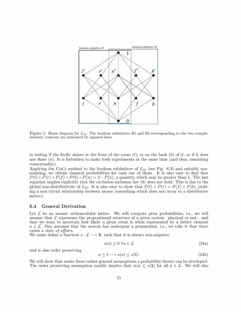
There are many systems of interest which can be represented by finite lattices. Many toy modelsserve to illustrate special features of different theories. Let us start first by analyzing L12, a nondistributive lattice which may be considered as the union of two incompatible experiments [64].The Hasse diagram of L12 is represented in Fig. 6.3. An example of L12 is provided by a fireflywhich flies inside a room. The first experiment is to test if the firefly shines on the right side(r) of the room, or on the left (l), or if it does not shine at all (n). Other experiment consists

14

Boolean sublattice B1 Boolean sublattice B2

Figure 1: Hasse diagram for L12. The boolean sublattices B1 and B2 corresponding to the two comple-mentary contexts are indicated by squared lines.

in testing if the firefly shines at the front of the room (f), or on the back (b) of it, or if it doesnot shine (n). It is forbidden to make both experiments at the same time (and thus, emulatingcontextuality).Applying the Cox’s method to the boolean sublattices of L12 (see Fig. 6.3) and suitably nor-malizing, we obtain classical probabilities for each one of them. It is also easy to find thatP (l)+P (r)+P (f)+P (b)+P (n) = 2−P (n), a quantity which may be greater than 1. The lastequation implies explicitly that the exclusion-inclusion law (6) does not hold. This is due to theglobal non-distributivity of L12. It is also easy to show that P (l) + P (r) = P (f) + P (b), yield-ing a non trivial relationship between atoms (something which does not occur in a distributivelattice).

6.4 General Derivation

Let L be an atomic orthomodular lattice. We will compute prior probabilities, i.e., we willassume that L represents the propositional structure of a given system –physical or not–, andthat we want to ascertain how likely a given event is when represented by a lattice elementa ∈ L. One assumes that the system has undergone a preparation, i.e., we take it that thereexists a state of affairs.We must define a function s : L −→ R, such that it is always non-negative

s(a) ≥ 0 ∀a ∈ L (24a)

and is also order preservinga ≤ b −→ s(a) ≤ s(b). (24b)

We will show that under these rather general assumptions a probability theory can be developed.The order preserving assumption readily implies that s(a) ≤ s(1) for all a ∈ L. We will also

15

assume that s(1) = K, a finite real number.Now, as an ortholattice is complemented (Eqs. (1)), we will always have that ¬¬a = a for alla ∈ L. Accordingly,

s(¬¬a) = s(a), (25)

for all a. Next, it is also reasonable to assume that s(¬a) is a function of s(¬a), say s(¬a) =g(s(a)). Thus, Eqs. (1a) and (25) imply

g(g(s(a))) = s(a), (26)

or, in other words,

g(g(x)) = x, (27)

for positive x. A family of functions which satisfy (26) are g(x) = x and g(x) = c − x, wherec is a real constant3. We discard the first possibility because if true, we would have s(0) =s(¬1) = g(s(1)) = s(1). But if s(0) = s(1), because of 0 ≤ x ≤ 1 for all x ∈ L, we haves(0) = s(x) = s(1), and our measure would be trivial. Thus, the only non-trivial option —upto rescaling— is s(¬a) = c− s(a).Now, let us see what happens with the “∨” operation. As L is orthocomplemented, the orthogo-nality notion for elements is available (see Section 2.1). If a, b ∈ L and a⊥b, because of (1b), wehave that a∧ b = 0. Thus, it is reasonable to assume that s(a∨ b) is a function of s(a) and s(b)only, i.e., s(a∨ b) = f(s(a), s(b)). By associativity of the “∨” operation, (a∨ b)∨ c = a∨ (b∨ c)for any a, b, c ∈ L, and this implies then that s((a ∨ b) ∨ c) = s(a ∨ (b ∨ c)). If a, b, and care orthogonal, we will have for the left hand side s((a ∨ b) ∨ c) = f(f(s(a), s(b)), s(c)) ands(a ∨ (b ∨ c)) = f(s(a), f(s(b), s(c))) for the right hand side. Thus,

f(f(s(a), s(b)), s(c)) = f(s(a), f(s(b), s(c))), (28)

or, in a simpler form

f(f(x, y), z) = f(x, f(y, z)), (29)

with x, y, and z positive real numbers. As shown in [60], the only solution (up to re-scaling) of(29) is f(x, y) = x+ y. We have thus shown that if a⊥b

s(a ∨ b) = s(a) + s(b), (30)

and we will also have

s(a1 ∨ a2 · · · ∨ an) = s(a1) + s(b2) + · · · + s(an), (31)

whenever a1, a2, · · · , an are pairwise orthogonal. Suppose now that aii∈N is a family ofpairwise orthogonal elements of L. For any finite n, we have that a1∨a2∨· · ·∨an ≤ 1, and thuss(a1 ∨ a2 ∨ · · · ∨ an) = s(a1) + s(b2) + · · ·+ s(an) ≤ s(1) = K. Then, sn = s(a1 ∨ a2 ∨ · · · ∨ an)is a monotone sequence bounded from above, and thus it converges to a real number. As∨aii∈N = limn−→∞

∨ni=1 ai, we can write

s(∨

aii∈N) =∞∑

i=1

s(ai). (32)

3There are additional solutions to this equation, but, if we suitably choose scales, we can disregard them forthese two cases. For a discussion on re-scaling of measures, their meaning and validity, see [17].

16

In any orthomodular lattice we have 1⊥0 (because 0 ≤ ¬1 = 0), and 1 ∨ 0 = 1. Thus,s(1 ∨ 0) = s(1) = s(1) + s(0). Accordingly, s(0) = 0. As ¬1 = 0, s(0) = c − s(1). Thus,s(1) = c and then, c = K. We will not lose generality if we assume the normalization conditionK = 1.

The results of this section show that in any orthomodular lattice, a reasonable measure s ofplausibility of a given event must satisfy that, for any orthogonal denumerable family aii∈N,one has (up to rescaling)

s(∨

aii∈N) =∞∑

i=1

s(ai) (33a)

s(¬a) = 1− s(a) (33b)

s(0) = 0. (33c)

Why do Eqs. (33) define non-classical (non-Kolmogorovian) probability measures? In a non-distributive orthomodular lattice there always exist elements a and b such that

(a ∧ b) ∨ (a ∧ ¬b) < a, (34)

so that (using (a∧¬b)⊥(a∧ b)), s((a∧¬b)∨ (a∧ b)) = s(a∧¬b)+s(a∧ b) ≤ s(a). The inequalitycan be strict, as the quantum case shows. But in any classical probability theory, by virtue ofthe inclusion-exclusion principle (Eqn. (7)), we always have s(a ∧ ¬b) + s(a ∧ b) = s(a). Thissimple fact shows that our measures will be non-classical in the general case.

In this way, we provide an answer to the problem posed by von Neumann and discussed inSection 4: the algebraic and logical properties of the operational event structure determine upto rescaling the general form of the probability measures which can be defined over the lattice.Accordingly, we did present a generalization of the Cox method to non-boolean structures,namely orthomodular lattices, and then we have indeed deduced a generalized probabilitytheory.

Remark that boolean lattices are also orthomodular. This means that our derivation is a gener-alization of that of Cox, and when we face a boolean structure, classical probability theory willbe deduced exactly as in [16, 17].Another important remark is that -as the reader may check- the derivation presented here isalso valid for σ-orthocomplete orthomodular posets (see Section 2 of this work), and thus, ofgreat generality. Indeed, in these structures the disjunction exists for denumerable collections oforthogonal elements and it is associative. This fact, together with orthocomplementation, makethe above results remain valid in these structures. But as it was mentioned in Section 2, σ-orthocomplete orthomodular posets are not lattices in the general case. In this way, we remarkthat the generalization of the Cox’s method goes well beyond lattice theory. Thus, yieldinga generalized probability calculus which includes the general physical approach presented forexample, in [4].

6.5 A general methodology

At this stage it is easy to envisage just how a general method could be developed. One firststarts by identifying the algebraic structure of the elementary tests of a given theory T . Theydetermine all observable quantities and, in the most important examples, they are endowedwith a lattice structure. Once the algebraic properties of the pertinent lattice are fixed, Cox’s

17

LQM L LCM

TQM TCMTTheory

Propositional

Latice

Probability

Theory

Cox’s

Method

von Neumann

PQM P PCM

Convex Set Of

States

Convex Structure

of Axioms

CQM C CCM

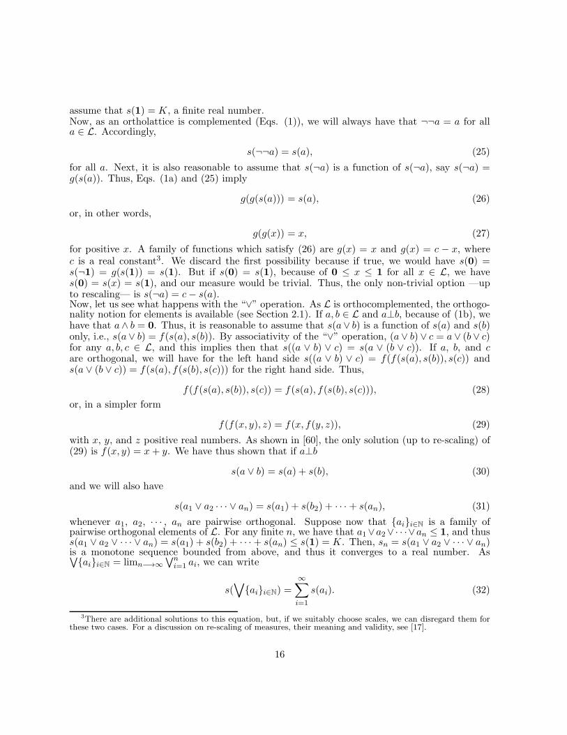
Figure 2: Schematic representation of the method proposed here. A general theory T determines via thevon Neumann approach the algebraic structure of the set of elementary tests. Then, by applying Cox’smethod, it is possible to determine the general properties of the canonical probability theory assigned toT . Next, by assigning particular values to prior probabilities of atoms, all states will be determined andthus, the form of C, the convex set of states. The quantum mechanical (QM) and the classical (CM)case are shown as the extreme instances of a vast family of theories.

method can be used to determine (up to rescaling) the general properties of prior probabilities.Of course, it does not predetermine the particular values that these probabilities might take onthe atoms of the theory. Such an specification would amount to determine a particular state ofthe system under scrutiny. The whole set of these states can be rearranged to yield a convexset. The path we have followed here is illustrated in Fig. 6.5, with the classical and quantumcases as extreme examples of a vast family.The method described in this work can be seen as a general epistemological background for ahuge family of scientific theories. In order to have a (quantitative) scientific theory, we must beable to make predictions on certain events of interest. Events are regarded here as propositionssusceptible of being tested. Thus, one starts from an inferential calculus which allows for quanti-fying the degree of belief on the certainty of an event x, if it is known that event y has occurred.The crucial point is that event structures are not always organized as boolean lattices (QM beingperhaps the most spectacular example). Thus, in order to determine the general properties ofthe probabilities of a given theory (and thus all possible states by specifying particular valuesof prior probabilities on the atoms), we must apply Cox’s method to lattices more general thanboolean ones.

7 Conclusions

By complementing the results presented in [24, 19, 20, 21, 25, 26, 28], in this work we showed thatit is possible to combine Cox’s method for the foundations of classical probability theory and theOQL approach, in order to give an alternative derivation of what is known as non-kolmogorovian(or non commutative) probability theory [4, 8].

18

Most physical probabilistic theories of interest can be endowed with orthomodular lattices. Theelements of these lattices represent the events of that theory. As in [20, 21], we have studied howthe algebraic properties of the lattices determine —up to rescaling— the general form of theprobabilities associated to the given physical theory. In this way, we provided a new formulationof the approach to physics based on non-kolmogorovian probability theory [4].

Differently from [24, 19, 20, 21, 25, 26, 28], in this work we have focused on the application ofthe Cox’s method to the von Neumann’s lattice of projection operators in a separable Hilbertspace and general orthomodular lattices as well, studying their particularities. In doing so,we obtained the von Neumann’s axioms of quantum probabilities, and thus (using Gleason’stheorem), quantum probabilities. In this way, our approach includes quantummixtures explicitlyand naturally.

It is interesting to remark (as in [20, 21]) that this construction is not necessarily restricted tophysics; any probabilistic theory endowed with a lattice structure of events will follow the sameroute.

We have also found that the method can be easily extended to σ-orthomodular posets (whichare not lattices in the general case), and thus, it contains generalizations of QM.

In deriving quantum probability out of the lattice properties, we have shown in a direct wayhow non-distributivity forbids the derivation of a Kolmogorovian probability. This sheds lighton the structure of quantum probabilities and on their differences with the classical case. Inparticular, we have shown that the properties of the underlying algebraic structure imply thatthe inclusion-exclusion principle is not valid for the von Neumann’s lattice. And, moreover, thatit can also fail in the more general framework of orthomodular (non-distributive) lattices. Wehave shown the explicit violation of the inclusion-exclusion principle for the finite example ofthe Chinese lantern and also for a non trivial relationship between atoms.

Furthermore, we have provided a non-trivial connection between the Cox’s approach and theproblem posed by von Neumann regarding the axiomatization of probabilities. This is a novelperspective on the origin and axiomatization of the probabilities which appear in quantumtheory. We believe that -far from being a definitive answer to the interpretation of quantumprobabilities- this is an interesting topic to be further investigated.

Using Cox’s approach, Shanon’s entropy can be deduced as a natural measure of informationover the boolean algebra of classical propositions [17, 28, 25]. We will provide a detailed studyof what happens with orthomodular latices elsewhere.

The strategy followed in this work suggests that we are at the gates of a great generalization.The general rule for constructing probabilities would read as follows:

• 1 - We start by identifying the operational logic of our physical system. The characteristicsof this “empirical” logic depends both on physical properties of the system and on theelection of the properties that we assume in order to study the system. This can be donein a standard way, and the method is provided by the OQL approach.

• 2 - Once the operational logic is identified, the symmetries of the lattice are used to de-fine the properties of the “degree of implication” function, which will turn out to be theprobability function associated to that particular logic. Remark that the same physicalsystem may have different propositional structures, depending of the election of the ob-servers. For example, if we look at the observable “electron’s” charge, we will face classicalpropositions, but if wee look at its momentum and position, we will have a non-booleanlattice.

19

This method is not only of physical interest, but also of mathematical one, because one is solvingthe problem of characterizing probability measures over general lattices (and other structuresas well). A final remark: our approach deviates from that of Cox, in the sense that we look foran empirical logic which would be intrinsic to the system under study, and because of that, notonly referred to our ignorance about it, but to assumptions about its nature. But this is not aproblem, but an advantage: any problem which can be transformed into the language of latticetheory (or the more general framework of σ-othocomplemented orthomodular posets) may fallinto this scheme, and a probability theory can be developed using the method described in thiswork.

Acknowledgements This work was partially supported by the grants PIP No 6461/05 amd1177 (CONICET). Also by the projects FIS2008-00781/FIS (MICINN) - FEDER (EU) (Spain,EU). The contribution of F. Holik to this work was done during his postdoctoral stance (CON-ICET) at Universidad Nacional de La Plata, Instituto de Fısica (IFLP-CCT-CONICET), C.C.727, 1900 La Plata, Argentina.

References

[1] G. Birkhoff and J. von Neumann, Annals Math. 37 (1936) 823-843.

[2] Dov M. Gabbay, JohnWoods, The Many Valued and Nonmonotonic Turn in Logic (Elsevier,Amsterdam, 2007), p. 205.

[3] M. Redei “The Birkhoff-von Neumann Concept of quantum Logic”, in Handbook of Quan-tum Logic and Quantum Structures, K. Engesser, D. M. Gabbay and D. Lehmann, eds.,Elsevier (2009).

[4] S. P. Gudder, Stochastic Methods in Quantum Mechanics North Holland, New York - Oxford(1979).

[5] S. P. Gudder, in Mathematical Foundations of Quantum Theory, A. R. Marlow, ed., Aca-demic, New York, (1978).

[6] M. L. Dalla Chiara, R. Giuntini, and R. Greechie, Reasoning in Quantum Theory, KluwerAcad. Pub., Dordrecht, (2004).

[7] M. Redei, Quantum Logic in Algebraic Approach, Kluwer Academic Publishers, Dordrecht,(1998).

[8] M. Redei and S. Summers, Studies in History and Philosophy of Science Part B: Studiesin History and Philosophy of Modern Physics Volume 38, Issue 2, (2007) 390-417.

[9] G. Mackey Mathematical foundations of quantum mechanics New York: W. A. Benjamin(1963).

[10] E. Davies and J. Lewis, Commun. Math. Phys. 17, (1970) 239-260.

[11] M. Srinivas, J. Math. Phys. 16, (1975) 1672.

[12] J. Acacio de Barros and P. Suppes, arXiv:quant-ph/0001017v1 (2000).

20

[13] C. Anastopoulos, Annals Of Physics 313, (2004) 368-382.

[14] J. Rau, Annals Of Physics 324, (2009) 2622-2637.

[15] Kolmogorov, A.N. Foundations of Probability Theory; Julius Springer: Berlin, Germany,(1933).

[16] Cox, R.T. Probability, frequency, and reasonable expectation. Am. J. Phys. 14, (1946) 1-13.

[17] Cox, R.T. The Algebra of Probable Inference; The Johns Hopkins Press: Baltimore, MD,USA, (1961).

[18] Boole, G. An Investigation of the Laws of Thought, Macmillan: London, UK, (1854).

[19] Knuth, K.H. Deriving laws from ordering relations. In Bayesian Inference and MaximumEntropy Methods in Science and Engineering, Proceedings of 23rd International Workshopon Bayesian Inference and Maximum Entropy Methods in Science and Engineering; Erick-son, G.J., Zhai, Y., Eds.; American Institute of Physics: New York, NY, USA, pp. 204-235(2004).

[20] Knuth, K.H. Measuring on lattices. In Bayesian Inference and Maximum Entropy Methodsin Science and Engineering, Proceedings of 23rd International Workshop on Bayesian In-ference and Maximum Entropy Methods in Science and Engineering; Goggans, P., Chan,C.Y., Eds.; American Institute of Physics: New York, NY, USA,; Volume 707, pp. 132-144(2004).

[21] Knuth, K.H. Valuations on lattices and their application to information theory. In Proceed-ings of the 2006 IEEE World Congress on Computational Intelligence, Vancouver, Canada,July (2006).

[22] E. T. Jaynes, Phys. Rev. Vol. 106, Number 4 (1957).

[23] E. T. Jaynes, Phys. Rev. Vol. 108, Number 2 (1957).

[24] A. Caticha, Phys. Rev. A 57 (1998) 1572-1582.

[25] Knuth, K.H. Lattice duality: The origin of probability and entropy. Neurocomputing 67C,(2005) 245-274.

[26] P. Goyal and K. Knuth, Symmetry 3 (2), (2011) 171-206, doi:10.3390/sym3020171.

[27] Goyal, P., Knuth, K.H. and Skilling, J., Phys. Rev. A 81 (2010) 022109.

[28] Knuth, K.H. and Skilling, arXiv:1008.4831v1 (2012).

[29] G. W. Mackey, Amer. Math. Monthly, Supplement 64 (1957) 45-57.

[30] J. M. Jauch, Foundations of Quantum Mechanics, Addison-Wesley, Cambridge, (1968).

[31] C. Piron, Foundations of Quantum Physics, Addison-Wesley, Cambridge, (1976).

[32] G. Kalmbach, Orthomodular Lattices, Academic Press, San Diego, (1983).

[33] G. Kalmbach, Measures and Hilbert Lattices, World Scientific, Singapore, (1986).

21

[34] V. Varadarajan, Geometry of Quantum Theory I, van Nostrand, Princeton, (1968).

[35] V. Varadarajan, Geometry of Quantum Theory II, van Nostrand, Princeton, (1970).

[36] J. R. Greechie, in Current Issues in Quantum Logic, E. Beltrameti and B. van Fraassen,eds., Plenum, New York, (1981) pp. 375-380.

[37] R. Giuntini, Quantum Logic and Hidden Variables, BI Wissenschaftsverlag, Mannheim,(1991).

[38] P. Ptak and S. Pulmannova, Orthomodular Structures as Quantum Logics, Kluwer AcademicPublishers, Dordrecht, (1991).

[39] E. G. Beltrametti and G. Cassinelli, The Logic of Quantum Mechanics, Addison-Wesley,Reading, (1981).

[40] A Dvurecenskij and S. Pulmannova, New Trends in Quantum Structures, Kluwer Acad.Pub., Dordrecht, (2000).

[41] Handbook Of Quantum Logic And Quantum Structures (Quantum Logic), Edited by K.Engesser, D. M. Gabbay and D. Lehmann, North-Holland (2009).

[42] D. Aerts and I. Daubechies, Lett. Math. Phys. 3 (1979) 11-17.

[43] D. Aerts and I. Daubechies, Lett. Math. Phys. 3 (1979) 19-27.

[44] D. Aerts, J. Math. Phys. 24 (1983) 2441.

[45] D. Aerts, Rep. Math. Phys 20 (1984) 421-428.

[46] D. Aerts, J. Math. Phys. 25 (1984) 1434-1441.

[47] B. Mielnik, Commun. Math. Phys. 9 (1968) 55-80.

[48] B. Mielnik, Commun. Math. Phys. 15 (1969) 1-46.

[49] B. Mielnik, Commun. Math. Phys. 37 (1974) 221-256.

[50] G. Ludwig, Commun. Math. Phys. 4, (1967) 331-348.

[51] G. Ludwig, Commun. Math. Phys. 9, (1968) 1-12.

[52] J. von Neumann, Mathematical Foundations of Quantum Mechanics, Princeton UniversityPress, 12th. edition, Princeton, (1996).

[53] M. Reed and B. Simon, Methods of modern mathematical physics I: Functional analysis,Academic Press, New York-San Francisco-London (1972).

[54] M. Soler, Communications in Algebra 23, (1995) 219-243.

[55] A. Wilce, Quantum Logic and Probability Theory, The Stanford Encyclope-dia of Philosophy (Spring 2009 Edition), Edward N. Zalta (ed.), URL =http://plato.stanford.edu/archives/spr2009/entries/qt-quantlog/. Archive edition: Spring2009.

22

[56] H. Barnum, J. Barret, M. Leifer and A. Wilce, Phys. Rev. Lett. 99, 240501 (2007).

[57] H. Barnum and A. Wilce, arXiv:0908.2352v1 [quant-ph] (2009); Electronic Notes in Theo-retical Computer Science Volume 270, Issue 1, Pages 3-15,(2011).

[58] H. Barnum, R. Duncan and A Wilce, arXiv:1004.2920v1 [quant-ph] (2010).

[59] M. Redei, The Mathematical Intelligencer, 21 (4), (1999) 7-12.

[60] Aczel, J., Lectures on Functional Equations and Their Applications, Academic Press, NewYork, (1966).

[61] A. Gleason, J. Math. Mech. 6, (1957) 885-893.

[62] D. Buhagiar, E. Chetcuti and A. Dvurecenskij, Found. Phys. 39, 550-558 (2009).

[63] N. Chomsky, IRE Transactions on Information Theory 2, 113 (1956).

[64] K. Svozil, Quantum Logic, Springer-Verlag, Singapore, (1998).

23