FEC 522: Financial Econometrics II - hs-stat · FEC 522: Financial Econometrics II Harald...
44
FEC 522: Financial Econometrics II Harald Schmidbauer c Harald Schmidbauer & Angi R¨ osch, 2011
Transcript of FEC 522: Financial Econometrics II - hs-stat · FEC 522: Financial Econometrics II Harald...

FEC 522:Financial Econometrics II
Harald Schmidbauer
c© Harald Schmidbauer & Angi Rosch, 2011

About These Slides
• The present slides are not self-contained; they need to be explained anddiscussed.
• Even though being a “work in progress” and subject to revision, theslides constitute copyrighted material.If you want to reproduce or copy anything from the slides, please ask:
Harald Schmidbauer harald at hs-stat dot comAngi Rosch angi at angi-stat dot com
• The slides were produced using LATEX (www.latex-project.org)and R (the R project; www.R-project.org) on a GNU/Linux system.
• R files used for this course are available upon request.
c© Harald Schmidbauer & Angi Rosch, 2011 About these slides 2/44

Chapter 5:
GARCH Processes
c© Harald Schmidbauer & Angi Rosch, 2011 5. GARCH Processes 3/44

5.1 Introduction
GARCH models: scope and outlook.
• There is usually a certain form of heteroskedasticity in a
series of returns.
• High volatility today can lead to high volatility tomorrow.
• Variances today and tomorrow are somehow related.
• For a time series (Xt) which is centered at 0, it holds that
var(Xt) = E(X2t ).
• This form of heteroskedasticity implies that there will be
autocorrelation in squared returns.
c© Harald Schmidbauer & Angi Rosch, 2011 5. GARCH Processes 4/44

5.1 Introduction
Example: IMKB 100 — the level series.
c© Harald Schmidbauer & Angi Rosch, 2011 5. GARCH Processes 5/44

5.1 Introduction
Example: IMKB 100 — the return series.
c© Harald Schmidbauer & Angi Rosch, 2011 5. GARCH Processes 6/44

5.1 Introduction
Example: IMKB 100 — acf of the return series.
0 5 10 15 20 25 30
0.0
0.2
0.4
0.6
0.8
1.0
AC
F
c© Harald Schmidbauer & Angi Rosch, 2011 5. GARCH Processes 7/44

5.1 Introduction
Example: IMKB 100 — acf of the squared return series.
0 5 10 15 20 25 30
0.0
0.2
0.4
0.6
0.8
1.0
AC
F
c© Harald Schmidbauer & Angi Rosch, 2011 5. GARCH Processes 8/44

5.1 Introduction
GARCH models: scope and outlook.
• GARCH models are a class of stochastic processes which
allow for this kind of heteroskedasticity.
• As before, the philosophy is:
Find a stochastic model which may have created the
observed series.
c© Harald Schmidbauer & Angi Rosch, 2011 5. GARCH Processes 9/44

5.2 Definition
GARCH: Definition.
A GARCH(p, q) process (εt) is defined as
εt = νt ·√ht, (νt): white noise with σ2
ν = var(νt) = 1,
and
ht = α0 +
q∑i=1
αiε2t−i︸ ︷︷ ︸
ARCH term
+
p∑i=1
βiht−i︸ ︷︷ ︸GARCH term
with parameters α0, α1, . . . , αq, β1, . . . , βp ≥ 0
and∑qi=1αi +
∑pi=1 βi < 1.
c© Harald Schmidbauer & Angi Rosch, 2011 5. GARCH Processes 10/44

5.2 Definition
GARCH: Some first comments.
• The GARCH is a model for heteroskedastic time series.
• GARCH stands for generalized autoregressive conditional
heteroskedasticity .
• The GARCH model was first developed by Engle (1982) and
Bollerslev (1986).
• A GARCH process is stationary. (Heteroskedasticity need
not be a reason for non-stationarity.)
c© Harald Schmidbauer & Angi Rosch, 2011 5. GARCH Processes 11/44

5.2 Definition
GARCH: Some first comments. — GARCH(1, 1):
εt = νt ·√ht, (νt): white noise with σ2
ν = var(νt) = 1,
ht = α0 + α1ε2t−1︸ ︷︷ ︸
ARCH term
+ β1ht−1︸ ︷︷ ︸GARCH term
with parameters α0, α1, β1 ≥ 0 and α1 + β1 < 1.
• Heteroskedasticity comes from the ht term.
• The term ht represents the one-period ahead forecast of the
variance.
• The term νt represents “news”, “shocks”, “residuals”.
c© Harald Schmidbauer & Angi Rosch, 2011 5. GARCH Processes 12/44

5.3 Conditional Heteroskedasticity
Conditional and unconditional moments of ARCH(1).
• Let’s now consider an ARCH(1) process:
εt = νt ·√α0 + α1ε2t−1
with var(νt) = 1, α0 > 0, 0 < α1 < 1.
• Our program:
– look at the unconditional moments,
– look at the conditional moments.
c© Harald Schmidbauer & Angi Rosch, 2011 5. GARCH Processes 13/44

5.3 Conditional Heteroskedasticity
Unconditional moments of ARCH(1).
• The model is:
εt = νt ·√α0 + α1ε2t−1
• Unconditional expectation:
E(εt) = E(νt) · E(√
α0 + α1ε2t−1
)= 0
c© Harald Schmidbauer & Angi Rosch, 2011 5. GARCH Processes 14/44

5.3 Conditional Heteroskedasticity
Unconditional moments of ARCH(1).
• The model is:
εt = νt ·√α0 + α1ε2t−1
• Unconditional variance:
var(εt) = E(ε2t) = E(ν2t ) · E(α0 + α1ε
2t−1
)=
α0
1− α1
• Unconditional correlation:
E(εt · εt+s) = 0, so that cor(εt, εt+s) = 0 for s ≥ 1.
c© Harald Schmidbauer & Angi Rosch, 2011 5. GARCH Processes 15/44

5.3 Conditional Heteroskedasticity
Conditional moments of ARCH(1).
• The model is:
εt = νt ·√α0 + α1ε2t−1
• Conditional expectation:
E(εt|εt−1, . . .) = E(νt) · E(√
α0 + α1ε2t−1
)= 0
c© Harald Schmidbauer & Angi Rosch, 2011 5. GARCH Processes 16/44

5.3 Conditional Heteroskedasticity
Conditional moments of ARCH(1).
• The model is:
εt = νt ·√α0 + α1ε2t−1
• Conditional variance:
var(εt|εt−1, . . .) = E(ε2t |εt−1) = α0 + α1ε2t−1 = ht
• This depends on εt−1! The ARCH is therefore a conditional
variance model.
• There will be positive autocorrelation in the process (ε2t).
c© Harald Schmidbauer & Angi Rosch, 2011 5. GARCH Processes 17/44

5.4 Simulation of a GARCH Process
The R code for simulating a GARCH(1,1) process.
a0 = 0.5; a1 = 0.3; b1 = 0.65
nu = rnorm(550)
epsi = rep(0, 550)
h = rep(0, 550)
for (i in 2:550) {
h[i] = a0 + a1 * epsi[i-1]^2 + b1 * h[i-1]
epsi[i] = nu[i] * sqrt(h[i])
}
epsi = epsi[51:550]
c© Harald Schmidbauer & Angi Rosch, 2011 5. GARCH Processes 18/44

5.4 Simulation of a GARCH Process
A simulated series.
0 100 200 300 400 500
−10
−5
05
10
c© Harald Schmidbauer & Angi Rosch, 2011 5. GARCH Processes 19/44

5.4 Simulation of a GARCH Process
Acf of the series and of the series of squares.
0 5 10 15 20 25
−0.
20.
20.
40.
60.
81.
0
0 5 10 15 20 25
0.0
0.2
0.4
0.6
0.8
1.0
c© Harald Schmidbauer & Angi Rosch, 2011 5. GARCH Processes 20/44

5.4 Simulation of a GARCH Process
Histogram of the distribution.
−10 −5 0 5 10
0.00
0.05
0.10
0.15
0.20
skewness: −0.250
s.e.: 0.34
kurtosis: 3.428
s.e.: 0.68
c© Harald Schmidbauer & Angi Rosch, 2011 5. GARCH Processes 21/44

5.5 Combining ARMA & GARCH
The purpose of combining ARMA and GARCH.
We have seen:
• ARMA models are conditional expectation models.
• Autocorrelation in the return series indicates that ARMA
may be appropriate.
• GARCH models are conditional variance models.
• Autocorrelation in the squared return series indicates that
GARCH may be appropriate.
c© Harald Schmidbauer & Angi Rosch, 2011 5. GARCH Processes 22/44

5.5 Combining ARMA & GARCH
The purpose of combining ARMA and GARCH.
The conclusion is:
• If there is autocorrelation in the series as well as in the
squared series, a combination of ARMA and GARCH may be
appropriate.
c© Harald Schmidbauer & Angi Rosch, 2011 5. GARCH Processes 23/44

5.5 Combining ARMA & GARCH
A mixed ARMA and GARCH model.
This is a process (Xt) defined as
a(L)Xt = c+ β(L)εt,
where
• a(L) is a polynomial of degree p in L,
• β(L) is a polynomial of degree q in L,
• (εt) is a GARCH process.
c© Harald Schmidbauer & Angi Rosch, 2011 5. GARCH Processes 24/44
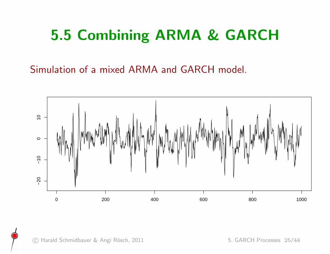
5.5 Combining ARMA & GARCH
Simulation of a mixed ARMA and GARCH model.
0 200 400 600 800 1000
−20
−10
010
c© Harald Schmidbauer & Angi Rosch, 2011 5. GARCH Processes 25/44

5.5 Combining ARMA & GARCH
Acfs of the simulated series and its squares.
0 5 10 15 20 25 30
0.0
0.2
0.4
0.6
0.8
1.0
0 5 10 15 20 25 30
0.0
0.2
0.4
0.6
0.8
1.0
c© Harald Schmidbauer & Angi Rosch, 2011 5. GARCH Processes 26/44

5.6 Examples
DJIA: the level series.
c© Harald Schmidbauer & Angi Rosch, 2011 5. GARCH Processes 27/44

5.6 Examples
DJIA: the return series.
c© Harald Schmidbauer & Angi Rosch, 2011 5. GARCH Processes 28/44

5.6 Examples
DJIA: acf of return series, squared return series.
0 5 10 15 20 25 30
0.0
0.2
0.4
0.6
0.8
1.0
AC
F
0 5 10 15 20 25 30
0.0
0.2
0.4
0.6
0.8
1.0
AC
F
c© Harald Schmidbauer & Angi Rosch, 2011 5. GARCH Processes 29/44

5.6 Examples
DJIA: fitting a GARCH model. (Mean return: 0.022)
Coefficient(s):
Estimate Std. Error t value Pr(>|t|)
a0 0.005481 0.002682 2.044 0.041 *
a1 0.056106 0.009821 5.713 1.11e-08 ***
b1 0.936337 0.011614 80.619 < 2e-16 ***
---
Signif. codes: 0 ’***’ 0.001 ’**’ 0.01 ’*’ 0.05 ’.’ 0.1 ’ ’ 1
Diagnostic Tests:
Jarque Bera Test
data: Residuals
X-squared = 4.2215, df = 2, p-value = 0.1211
Box-Ljung test
data: Squared.Residuals
X-squared = 3.6251, df = 1, p-value = 0.05692
c© Harald Schmidbauer & Angi Rosch, 2011 5. GARCH Processes 30/44
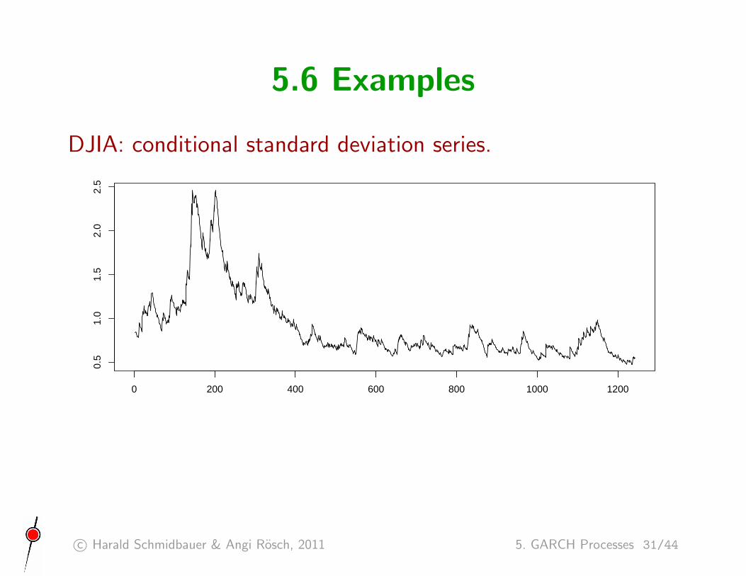
5.6 Examples
DJIA: conditional standard deviation series.
0 200 400 600 800 1000 1200
0.5
1.0
1.5
2.0
2.5
c© Harald Schmidbauer & Angi Rosch, 2011 5. GARCH Processes 31/44

5.6 Examples
Siemens: the level series.
c© Harald Schmidbauer & Angi Rosch, 2011 5. GARCH Processes 32/44

5.6 Examples
Siemens: the return series.
c© Harald Schmidbauer & Angi Rosch, 2011 5. GARCH Processes 33/44

5.6 Examples
Siemens: acf of return series, squared return series.
0 5 10 15 20 25 30
0.0
0.2
0.4
0.6
0.8
1.0
AC
F
0 5 10 15 20 25 30
0.0
0.2
0.4
0.6
0.8
1.0
AC
F
c© Harald Schmidbauer & Angi Rosch, 2011 5. GARCH Processes 34/44

5.6 Examples
Siemens: fitting a GARCH model. (Mean return: 0.071)
Coefficient(s):
Estimate Std. Error t value Pr(>|t|)
a0 0.030456 0.009857 3.090 0.00200 **
a1 0.056059 0.009051 6.193 5.89e-10 ***
b1 0.930380 0.011470 81.117 < 2e-16 ***
---
Signif. codes: 0 ’***’ 0.001 ’**’ 0.01 ’*’ 0.05 ’.’ 0.1 ’ ’ 1
Diagnostic Tests:
Jarque Bera Test
data: Residuals
X-squared = 214.8504, df = 2, p-value < 2.2e-16
Box-Ljung test
data: Squared.Residuals
X-squared = 0.0023, df = 1, p-value = 0.9617
c© Harald Schmidbauer & Angi Rosch, 2011 5. GARCH Processes 35/44

5.6 Examples
Siemens: conditional standard deviation series.
0 200 400 600 800 1000
1.0
1.5
2.0
2.5
3.0
3.5
c© Harald Schmidbauer & Angi Rosch, 2011 5. GARCH Processes 36/44

5.6 Examples
Brent crude oil: the level series.
c© Harald Schmidbauer & Angi Rosch, 2011 5. GARCH Processes 37/44

5.6 Examples
Brent crude oil: the return series.
c© Harald Schmidbauer & Angi Rosch, 2011 5. GARCH Processes 38/44

5.6 Examples
Brent crude oil: acf of return series, squared return series.
0 5 10 15 20 25 30
0.0
0.2
0.4
0.6
0.8
1.0
AC
F
0 5 10 15 20 25 30
0.0
0.2
0.4
0.6
0.8
1.0
AC
F
c© Harald Schmidbauer & Angi Rosch, 2011 5. GARCH Processes 39/44

5.6 Examples
Brent crude oil: fitting a GARCH model. (Mean return: 0.117)
Coefficient(s):
Estimate Std. Error t value Pr(>|t|)
a0 0.32744 0.15108 2.167 0.03021 *
a1 0.03889 0.01309 2.971 0.00297 **
b1 0.89014 0.04220 21.092 < 2e-16 ***
---
Signif. codes: 0 ’***’ 0.001 ’**’ 0.01 ’*’ 0.05 ’.’ 0.1 ’ ’ 1
Diagnostic Tests:
Jarque Bera Test
data: Residuals
X-squared = 62.6624, df = 2, p-value = 2.476e-14
Box-Ljung test
data: Squared.Residuals
X-squared = 2.3493, df = 1, p-value = 0.1253
c© Harald Schmidbauer & Angi Rosch, 2011 5. GARCH Processes 40/44

5.6 Examples
Brent crude oil: conditional standard deviation series.
0 200 400 600 800 1000 1200
2.0
2.2
2.4
2.6
2.8
3.0
3.2
c© Harald Schmidbauer & Angi Rosch, 2011 5. GARCH Processes 41/44

5.7 Limitations
This GARCH: symmetric & univariate.
Limitations of the GARCH processes we have seen are:
• “News impact” on the variance is symmetric:
ε 7→ α0 + α1ε2 + β1σ
2
• This process is univariate.
This limits its scope to investigate volatility spillovers.
c© Harald Schmidbauer & Angi Rosch, 2011 5. GARCH Processes 42/44

5.7 Limitations
Example: Asymmetry in the DJIA return series.
• Is there empirical evidence for asymmetry in the series of
returns?
• We can now do the following:
– Make a scatterplot of rt and r2t+1.
(Our plot uses daily data , Apr 1981 through Sep 2008.)
– Plot a local regression line. (R: lowess)
– Look for asymmetry!
Simulated GARCH data would produce a symmetric line.
c© Harald Schmidbauer & Angi Rosch, 2011 5. GARCH Processes 43/44

5.7 Limitations
Example: Asymmetry in the DJIA return series.
c© Harald Schmidbauer & Angi Rosch, 2011 5. GARCH Processes 44/44