Feature selection by higher criticism thresholding...

on August 19, 2018http://rsta.royalsocietypublishing.org/Downloaded from

Phil. Trans. R. Soc. A (2009) 367, 4449–4470doi:10.1098/rsta.2009.0129

Feature selection by higher criticismthresholding achieves the optimal phase diagram

BY DAVID DONOHO1 AND JIASHUN JIN2,*1Department of Statistics, Stanford University, Stanford, CA 94305, USA

2Statistics Department, Carnegie Mellon University, Pittsburgh,PA 15213, USA

We consider two-class linear classification in a high-dimensional, small-sample-sizesetting. Only a small fraction of the features are useful, these being unknown to us,and each useful feature contributes weakly to the classification decision. This was calledthe rare/weak (RW) model in our previous study (Donoho, D. & Jin, J. 2008 Proc. NatlAcad. Sci. USA 105, 14 790–14 795). We select features by thresholding feature Z -scores.The threshold is set by higher criticism (HC). For 1 ≤ i ≤ N , let πi denote the p-valueassociated with the ith Z -score and π(i) denote the ith order statistic of the collectionof p-values. The HC threshold (HCT) is the order statistic of the Z -score correspondingto index i maximizing (i/N − π(i))/

√i/N (1 − i/N ). The ideal threshold optimizes the

classification error. In that previous study, we showed that HCT was numerically closeto the ideal threshold.

We formalize an asymptotic framework for studying the RW model, considering asequence of problems with increasingly many features and relatively fewer observations.We show that, along this sequence, the limiting performance of ideal HCT is essentiallyjust as good as the limiting performance of ideal thresholding. Our results describe two-dimensional phase space, a two-dimensional diagram with coordinates quantifying ‘rare’and ‘weak’ in the RW model. The phase space can be partitioned into two regions—onewhere ideal threshold classification is successful, and one where the features are so weakand so rare that it must fail. Surprisingly, the regions where ideal HCT succeeds and failsmake exactly the same partition of the phase diagram. Other threshold methods, such asfalse (feature) discovery rate (FDR) threshold selection, are successful in a substantiallysmaller region of the phase space than either HCT or ideal thresholding. The FDR andlocal FDR of the ideal and HC threshold selectors have surprising phase diagrams, whichare also described. Results showing the asymptotic equivalence of HCT with ideal HCTcan be found in a forthcoming paper (Donoho, D. & Jin, J. In preparation).

Keywords: asymptotic rare/weak model; false discovery rate; linear classification;phase diagram; Fisher’s separation measure; feature selection by thresholding

*Author for correspondence ([email protected]).

Electronic supplementary material is available at http://dx.doi.org/10.1098/rsta.2009.0129 or viahttp://rsta.royalsocietypublishing.org.

One contribution of 11 to a Theme Issue ‘Statistical challenges of high-dimensional data’.

This journal is © 2009 The Royal Society4449

mailto:[email protected]

http://dx.doi.org/10.1098/rsta.2009.0129

http://rspa.royalsocietypublishing.org

http://rsta.royalsocietypublishing.org/

4450 D. Donoho and J. Jin


1. Introduction

The modern era of high-throughput data collection creates data inabundance. Some devices—spectrometers and gene chips come to mind—automatically generate measurements on thousands of standard features of eachobservational unit.

What has not changed in science is the difficulty of obtaining goodobservational units. High-throughput devices do not help us to find and enrolqualified patients, or to catch exotic butterflies or to observe primate matingbehaviour. So the number of observational units—be they patients, butterflies ormatings—has not increased; it stays in the dozens or hundreds. However, each ofthose few observational units can now be subjected to a large battery of automaticfeature measurements.

Many of those automatically measured features will have little relevance to anygiven project. This new era of feature glut poses a needle-in-a-haystack problem:we must detect a relatively few valuable features among many useless ones.Unfortunately, the combination of small sample sizes (few observational units)and high dimensions (many feature measurements) makes it hard to tell needlesfrom straw.

Orthodox statistical methods assumed quite a different set of conditions: moreobservations than features, and all features highly relevant. Modern statisticalresearch has started to address this modern, unorthodox setting; such researchcomprised much of the activity in the recent six-month Newton Instituteprogramme Statistical Theory and Methods for Complex, High-Dimensional Data.

This paper examines the challenges that feature glut poses to linearclassification schemes. A new feature selection principle—higher criticism (HC)thresholding—and a new optimality property—optimality of the phase diagram—will be introduced.

(a) Multivariate normal classification

In the standard model of linear classifier training, we have labelled trainingsamples (Yi , Xi), i = 1, . . . , n, where each label Yi is ±1 and each feature vectorXi ∈ Rp. For simplicity, let us assume that the training set contains equalnumbers of +1 and −1 and that the feature vectors Xi ∈ Rp obey Xi ∼ N (Yiμ, Σ),i = 1, . . . , n, for an unknown mean contrast vector μ ∈ Rp; here Σ denotes thefeature covariance matrix and n is the training set size. In this simple setting,one normally uses linear classifiers to classify an unlabelled test vector X ,taking the general form L(X ) = ∑p

j=1 w( j)X ( j), with ‘feature weights’ w = (w( j) :j = 1, . . . , p).

Classical theory going back to R. A. Fisher shows that the optimal classifierhas feature weights w ∝ Σ−1μ (Anderson 2003). However, modern feature glutrenders Fisher’s formula inapplicable.

(b) When p is larger than n

Frequently, in modern settings, the number p of measurements exceeds thenumber n of observational units. Naive application of the formula w ∝ Σ−1μ toempirical data in the p > n setting is then problematic, at a minimum, because

Phil. Trans. R. Soc. A (2009)


Feature selection by HC thresholding 4451


the matrix of empirical feature covariances Covn,p(X ) is not invertible. Eventhe generalized inverse Covn,p(X )† gives weights wnaive ∝ Covn,p(X )†Covn,p(Y , X ),yielding ‘noisy’ classifiers with low accuracy.

A by-now standard response to this problem is simply to ignore featurecovariances, and to standardize the features to mean 0 and variance 1. In effect,one pretends that the feature covariance matrix Σ is the identity matrix, anduses the formula w( j) ∝ Cov(Y , X ( j)) (Bickel & Levina 2004; Fan & Fan 2008).Even after this reduction, further challenges remain.

(c) When features are rare and weak

When feature glut arises from promiscuous measurement, researchers cannotsay in advance which features will be useful in a given project. Moreover, althoughone hopes to find a single ‘silver bullet’ feature that reliably classifies, in all toomany projects the useful features are relatively rare and individually quite weak.

Such thinking motivated the following rare/weak (RW) feature model inDonoho & Jin (2008). Under this model, the following hold.

(i) Useful features are rare. The contrast vector μ is non-zero in only k outof p elements, where ε = k/p is small, i.e. close to zero. As an example,think of p = 10 000, k = 100, so ε = k/p = 0.01.

(ii) Useful features are weak. The non-zero elements of μ have commonamplitude μ0, which is assumed not to be ‘large’. ‘Large’ can be measuredusing τ = √

nμ0; values of τ in the range of 2–4 imply that correspondingvalues of μ are not large.

Since the elements X ( j) of the feature vector where the class contrast μ( j) = 0are entirely uninformative about the value of Y ( j), only the k features whereμ( j) = μ0 are useful. The problem is how to identify and benefit from thoserare/weak features.

We speak of ε and τ as the sparsity and strength parameters for the RWmodel, and refer to the RW(ε, τ) model. Models with a ‘sparsity’ parameter ε arecommon in estimation settings (Donoho et al. 1992; Donoho & Johnstone 1994;Johnstone & Silverman 2004), but not with the feature strength constraint τ .Also closely related to the RW model is work in multiple testing by Ingster andother authors (Ingster 1997; Jin 2003; Donoho & Jin 2004).

(d) Feature selection by thresholding

Feature selection—i.e. working only with an empirically selected subset offeatures—is a standard response to feature glut. We are supposing, as announcedin §1b, that feature correlations can be ignored and that features are alreadystandardized to variance 1. We therefore focus on the vector of feature Z -scores,with components Z ( j) = n−1/2 ∑

i YiXi( j), j = 1, . . . , p. These are the Z -scores oftwo-sided tests of H0,j : Cov(Y , X ( j)) = 0. Under our assumptions, Z ∼ N (θ , Ip)

with θ = √nμ and μ the feature contrast vector. Features with non-zero μ( j)

typically have significantly non-zero Z ( j), while all other features will have Z ( j)values largely consistent with the null hypothesis μ( j) = 0. In such a setting,selecting features with Z -scores above a threshold makes sense.





We identify three useful threshold functions: η�t (Z ), with � ∈ {clip, hard, soft}.

These are: clipping, ηclipt (Z ) = sgn(Z ) · 1{|z |>t}, which ignores the size of the

Z -score, provided it is large; hard thresholding, ηhardt (Z ) = Z · 1{|Z |>t}, which uses

the size of the Z -score, provided it is large; and soft thresholding, ηsoftt (z) =

sgn(Z )(|Z | − t)+, which uses a shrunken Z -score, provided it is large.

Definition 1.1. Let � ∈ {soft, hard, clip}. The threshold feature selectionclassifier makes its decision based on L�

t <> 0, where L�t (X ) = ∑p

j=1 w�t ( j)X ( j),

and w�t ( j) = η�

t (Z ( j)), j = 1, . . . , p.

In other words, the classifier sums across features with large training setZ -scores, and a simple function of the Z -score generates the feature weight.

Several methods for linear classification in bioinformatics follow this approach.The shrunken centroids method (Tibshirani et al. 2002) is a variant of softthresholding in this two-class setting. The highly cited methods in Golub et al.(1999) and Hedenfalk et al. (2001) are variants of hard thresholding. Clippingmakes sense in the theoretical setting of the RW model (since then the usefulfeatures all have the same strength) and is simpler to analyse than the othernonlinearities.

One crucial question remains: how to choose the threshold based on thedata? Popular methods for threshold choice include cross-validation (Tibshiraniet al. 2002), control of the false discovery rate (Abramovich & Benjamini 1995;Benjamini & Hochberg 1995; Abramovich et al. 2006; Donoho & Jin 2006) andcontrol of the local false discovery rate (Efron et al. 2001).

(e) Higher criticism

Recent work on multiple comparisons offers a new method of threshold choice.

(i) Higher criticism testing

Suppose that we have a collection of N p-values πi , which, under theglobal null hypothesis, are uniformly (independent and identically) distributed:πi ∼i.i.d. U [0, 1]. Consider the order statistics π(1) ≤ π(2) ≤ · · · ≤ π(N ). Under thenull hypothesis, these order statistics have the usual properties of uniform orderstatistics, including the asymptotic normality π(i) ∼approx Normal(i/N , i/N (1 −i/N )). HC forms a Z -score comparing π(i) with its mean under the null, and thenmaximizes over a wide range of i.

Definition 1.2 (HC testing (Donoho & Jin 2004)). The higher criticismobjective is

HC(i; π(i)) = √N

i/N − π(i)√i/N (1 − i/N )

. (1.1)

Fix α0 ∈ (0, 1) (e.g. α0 = 0.10). The higher criticism test statistic is HC∗ =max1≤i≤α0N HC(i; π(i)).

HC seems insensitive to the selection of α, in rare/weak situations; here wealways use α0 = 0.10.

Expressed in words, we look for the largest standardized discrepancy for anyπ(i) between the observed behaviour and the expected behaviour under the null.When this is large, the whole collection of p-values is not consistent with the





0

0

0 0.02 0.04 0.06 0.08 0.10

5(a)

(b)

(c)

0.05

0.10

5

10

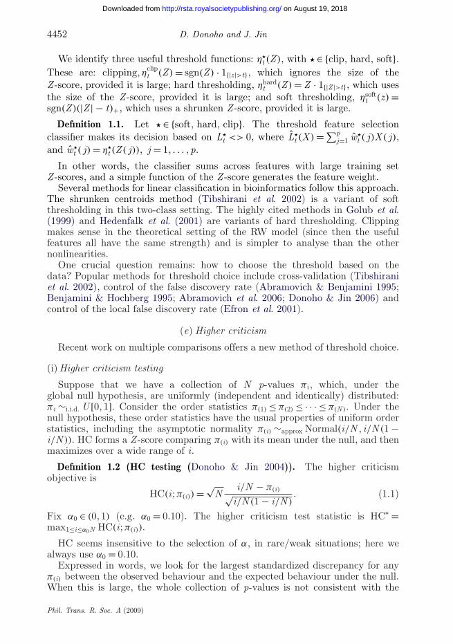
Figure 1. Illustration of HC thresholding. (a) The ordered |Z |-scores. (b) The corresponding orderedp-values in a PP plot. (c) The HC objective function in equation (1.1); this is largest at ı ≈ 0.007p.The x-axes are i/p. Vertical (red) lines indicate π(ı) in (b), and |Z |(ı) in (a).

global null hypothesis. The phrase ‘higher criticism’ is due to John Tukey, andreflects the shift in emphasis from single test results to the whole collectionof tests.

(ii) Higher criticism thresholding

We return to the classification setting in the previous sections. We have avector of feature Z -scores (Z ( j), j = 1, . . . , p). To apply HC notions, translate Z -scores into two-sided p-values, and maximize the HC objective over index i in theappropriate range. Define the feature p-values πi = Prob{|N (0, 1)| > |Z (i)|}, i =1, . . . , p; and define the increasing rearrangement π(i), the HC objective functionHC(i; π(i)), and the increasing rearrangement |Z |(i) correspondingly. Here is ourproposal.

Definition 1.3 (HC thresholding). Apply the HC procedure to the featurep-values. Let the maximum HC objective be achieved at index ı. The highercriticism threshold (HCT) is the value tHC = |Z |(ı). The HC threshold featureselector selects features with Z -scores exceeding tHC in magnitude.

Figure 1 illustrates the procedure. Figure 1a shows a sample of Z -scores, figure1b shows a probability–probability (PP) plot of the corresponding ordered p-values versus i/p, and figure 1c shows a standardized PP plot. The standardizedPP plot has its largest deviation from 0 at ı; and this generates thethreshold value.





(iii) Previously reported results for higher criticism threshold

Donoho & Jin (2008) reported several findings on the behaviour of HCT basedon numerical and empirical evidence. In the RW model, define the ideal thresholdas the optimal threshold based on full knowledge of the RW parameters ε and μ(see §2 below).

(i) The HCT threshold is numerically very close to the ideal threshold.(ii) In the case of very weak feature Z -scores, HCT has a false feature discovery

rate (FDR) substantially higher than other popular approaches, but afeature missed detection rate (MDR) substantially lower than those otherapproaches.

(iii) FDR and MDR of HCT closely match those of the ideal threshold.

In short, HCT has operating characteristics unlike those of popularthresholding schemes such as FDR thresholding (Abramovich & Benjamini 1995;Abramovich et al. 2006) and Bonferroni thresholding, but very similar to theideal ones.

(f ) Asymptotic rare/weak model, and the phase diagram

This paper reports a large-sample analysis of HCT and the RW model. Thenumber of observations n and the number of features p will tend to infinity in alinked fashion, with n remaining very small compared to p. (Empirical resultsin Donoho & Jin (2008) show that large-p theory is applicable at moderaten and p).

Definition 1.4. The phrase asymptotic rare/weak (ARW) model refers to thefollowing combined assumptions.

(i) Asymptotic setting. We consider a sequence of problems, with the numberof observations n and the number of features p both tending to ∞.

(ii) p dramatically larger than n. Along this sequence, n ∼ c(log p)γ for somepositive constants c and γ , so there are dramatically more features perobservational unit than there are observational units.

(iii) Increasing rarity. The sparsity ε tends to 0: ε = p−β , 0 < β < 1.(iv) Decreasing strength. The strength τ varies with n and p according

to τ = √2r log p, 0 < r < 1.

The symbol ARW(r , β; c, γ ) refers to the model combining these assumptions.

In this model, because r < 1, useful features are individually too weak todetect and, because 0 < β < 1, useful features are increasingly rare with increasingp, while increasing in total number with p. It turns out that c and γ areincidental, while r and β are the driving parameters. Hence, we always simplywrite ARW(r , β) below.

For many choices of (r , β), asymptotically successful classification is possible;for another large family of choices, it is impossible. To understand this fact,we use the concept of phase space, the two-dimensional domain, 0 < r , β < 1.We show that this domain is partitioned into two regions or ‘phases’. In the‘impossible’ phase, useful features are so rare and so weak that classification is





0.50 0.55 0.60 0.65 0.70 0.75 0.80 0.85 0.90 0.95 1.000

0.1

0.2

0.3

0.4

0.5

0.6

0.7

0.8

0.9

1.0

II

I

III

β

r

(1,1)

((β−r)/(2r), (β+r)/(4r))

(0,1/2) success

failure

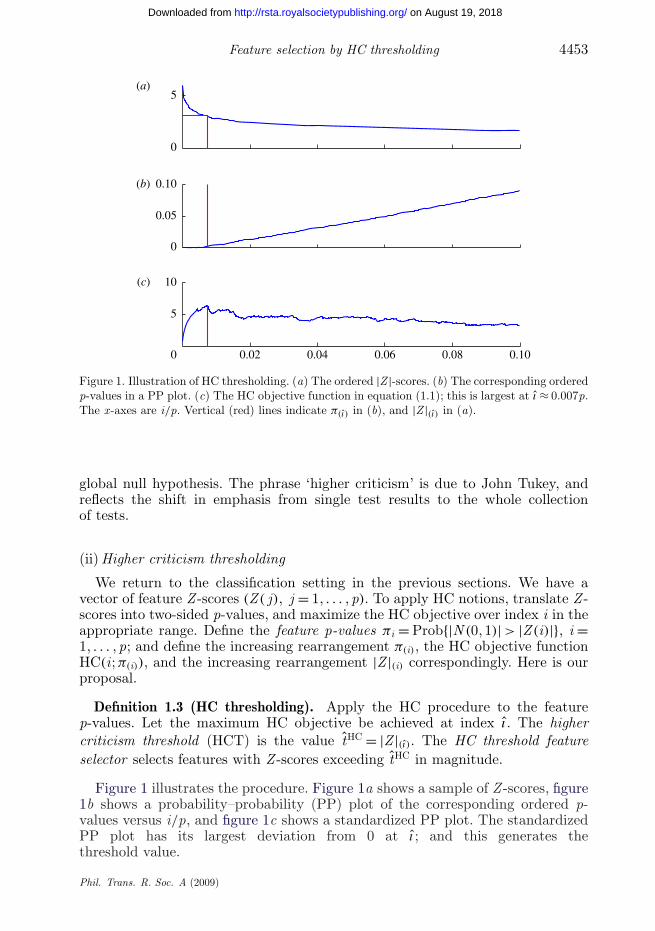
Figure 2. Phase diagram. The curve r = ρ∗(β) divides phase space into failure and success regions,and the latter further splits into three different regions I, II and III. Numbers in the brackets showlimits of ˜FDR and Lfdr at the ideal HCT as in theorem 3.7.

asymptotically impossible even with the ideal choice of threshold. In the ‘possible’phase, successfully separating the two groups is indeed possible—if one has accessto the ideal threshold. Figure 2 displays this domain and its partition into phases.Because of the partition into two phases, we also call this display the phasediagram. An explicit formula for the graph r = ρ∗(β) bounding these phases isgiven in equation (3.2) below.

The phase diagram provides a convenient platform for comparing differentprocedures. A threshold choice is optimal if it gives the same partition of phasespace as the one obtained with the ideal choice of threshold.

How does HCT compare to the ideal threshold, and what partition in the phasespace does HCT yield? For reasons of space, we focus in this paper on the ideal HCthreshold, which is obtained upon replacing the empirical distribution of featureZ -scores by its expected value. The ideal HC threshold is thus the one that HCTis ‘trying to estimate’.

The central surprise of our story is that ideal HCT behaves surprisinglywell: the partition of phase space describing the two regions where idealthresholding fails and/or succeeds also describes the two regions where HCTfails and/or succeeds. The situation is depicted in table 1: here ‘succeeds’ meansasymptotically zero misclassification rate, and ‘fails’ means asymptotically 50per cent misclassification rate.

In this sense of size of regions of success, HCT is just as good as the idealthreshold. Such statements cannot be made for some other popular thresholdingschemes, such as false discovery threshold selection. Even the very popular





Table 1. Comparison of ideal threshold and ideal HCT.

region property of ideal threshold property of ideal HCT

r < ρ∗(β) ideal threshold classifier fails ideal HCT failsr > ρ∗(β) ideal threshold classifier succeeds ideal HCT succeeds

cross-validated choice of threshold will fail if the training set size is bounded,while HCT will still succeed in the RW model in that case.

(g) Contents

The paper is organized as follows. Section 2 introduces a functional frameworkand several ideal quantities. These include the proxy classification error whereFisher’s separation (Sep) plays a key role, the ideal threshold as a proxy for theoptimal threshold, and the ideal HCT as a proxy of the HCT. Section 3 introducesthe main results on the asymptotic behaviour of the HC threshold under theasymptotic RW model, and the focal point is the phase diagram. Section 4outlines the basic idea behind the main results followed by the proofs. Section 5discusses the connection between the ideal threshold and the ideal HCT.Section 6 discusses the ideal behaviour of Bonferroni threshold feature selectionand FDR-controlling feature selection. Section 7 discusses the link between idealHCT and ordinary HCT, the finite-p phase diagram, and other appearances ofHC in recent literature.

This paper has three companions: Donoho & Jin (2008, in preparation) andJin (2009). The full proof of a broader set of claims, with a considerably moregeneral treatment, will appear in Donoho & Jin (in preparation) (see §7).

2. Fisher’s separation functional and ideal threshold

Suppose L is a fixed, non-random linear classifier, with decision boundary L <>0. Will L correctly classify the future realization (Y , X )? Suppose that Y = ±1are equiprobable and X ∼ N (Yμ, Ip). The misclassification probability can bewritten as:

P{YL(X ) < 0 | μ} = Φ(− 1

2Sep(L; μ)), (2.1)

where Φ denotes the standard normal distribution function and Sep(L; μ)measures the standardized interclass distance:

Sep(L; μ) = E{L(X ) | Y = 1} − E{L(X ) | Y = −1}SD(L(X ))

= 2∑

w( j)μ( j)(∑w( j)2

)1/2 = 2〈w, μ〉‖w‖2

. (2.2)

The ideal linear classifier Lμ with feature weights w ∝ μ and decision thresholdLμ <> 0 implements the likelihood ratio test. It also maximizes Sep, since, forevery other linear classifier L, Sep(L; μ) ≤ Sep(Lμ; μ) = 2‖μ‖2.





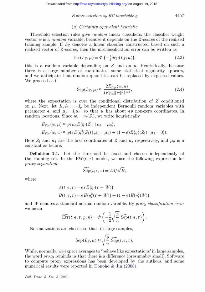
(a) Certainty equivalent heuristic

Threshold selection rules give random linear classifiers: the classifier weightvector w is a random variable, because it depends on the Z -scores of the realizedtraining sample. If LZ denotes a linear classifier constructed based on such arealized vector of Z -scores, then the misclassification error can be written as

Err(LZ , μ) = Φ(− 1

2Sep(LZ ; μ)); (2.3)

this is a random variable depending on Z and on μ. Heuristically, becausethere is a large number of coordinates, some statistical regularity appears,and we anticipate that random quantities can be replaced by expected values.We proceed as if

Sep(LZ ; μ) ≈ 2EZ |μ〈w, μ〉(EZ |μ‖w‖2)1/2

, (2.4)

where the expectation is over the conditional distribution of Z conditionedon μ. Next, let I1, I2, . . . , Ip be independent Bernoulli random variables withparameter ε, and μj = Ijμ0, so that μ has about εp non-zero coordinates, inrandom locations. Since wi = ηt(Zi), we write heuristically

EZ |μ〈w, μ〉 ≈ pεμ0E{ηt(Z1) | μ1 = μ0},EZ |μ〈w, w〉 ≈ p(εE{η2

t (Z1) | μ1 = μ0} + (1 − ε)E{η2t (Z1) | μ1 = 0}).

Here Z1 and μ1 are the first coordinates of Z and μ, respectively, and μ0 is aconstant as before.

Definition 2.1. Let the threshold be fixed and chosen independently ofthe training set. In the RW(ε, τ) model, we use the following expression forproxy separation:

Sep(t; ε, τ) = 2A/√

B,

where

A(t, ε, τ) = ετE{ηt(τ + W )},B(t, ε, τ) = εE{η2

t (τ + W )} + (1 − ε)E{η2t (W )},

and W denotes a standard normal random variable. By proxy classification errorwe mean

Err(t; ε, τ , p, n) = Φ

(−1

2

√pn

Sep(t, ε, τ)

).

Normalizations are chosen so that, in large samples,

Sep(LZ , μ) ≈√

pn

Sep(t, ε, τ).

While, normally, we expect averages to ‘behave like expectations’ in large samples,the word proxy reminds us that there is a difference (presumably small). Softwareto compute proxy expressions has been developed by the authors, and somenumerical results were reported in Donoho & Jin (2008).





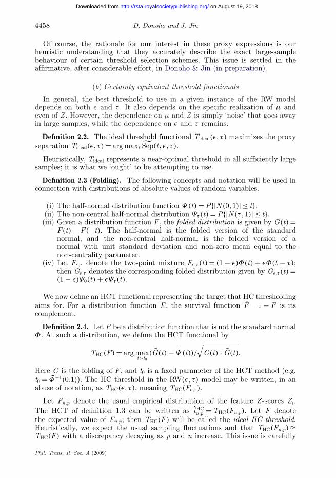
Of course, the rationale for our interest in these proxy expressions is ourheuristic understanding that they accurately describe the exact large-samplebehaviour of certain threshold selection schemes. This issue is settled in theaffirmative, after considerable effort, in Donoho & Jin (in preparation).

(b) Certainty equivalent threshold functionals

In general, the best threshold to use in a given instance of the RW modeldepends on both ε and τ . It also depends on the specific realization of μ andeven of Z . However, the dependence on μ and Z is simply ‘noise’ that goes awayin large samples, while the dependence on ε and τ remains.

Definition 2.2. The ideal threshold functional Tideal(ε, τ) maximizes the proxyseparation Tideal(ε, τ) = arg maxt Sep(t, ε, τ).

Heuristically, Tideal represents a near-optimal threshold in all sufficiently largesamples; it is what we ‘ought’ to be attempting to use.

Definition 2.3 (Folding). The following concepts and notation will be used inconnection with distributions of absolute values of random variables.

(i) The half-normal distribution function Ψ (t) = P{|N (0, 1)| ≤ t}.(ii) The non-central half-normal distribution Ψτ(t) = P{|N (τ , 1)| ≤ t}.(iii) Given a distribution function F , the folded distribution is given by G(t) =

F(t) − F(−t). The half-normal is the folded version of the standardnormal, and the non-central half-normal is the folded version of anormal with unit standard deviation and non-zero mean equal to thenon-centrality parameter.

(iv) Let Fε,τ denote the two-point mixture Fε,τ (t) = (1 − ε)Φ(t) + εΦ(t − τ);then Gε,τ denotes the corresponding folded distribution given by Gε,τ (t) =(1 − ε)Ψ0(t) + εΨτ (t).

We now define an HCT functional representing the target that HC thresholdingaims for. For a distribution function F , the survival function F = 1 − F is itscomplement.

Definition 2.4. Let F be a distribution function that is not the standard normalΦ. At such a distribution, we define the HCT functional by

THC(F) = arg maxt>t0

(G(t) − Ψ (t))/√

G(t) · G(t).

Here G is the folding of F , and t0 is a fixed parameter of the HCT method (e.g.t0 = Φ−1(0.1)). The HC threshold in the RW(ε, τ) model may be written, in anabuse of notation, as THC(ε, τ), meaning THC(Fε,τ ).

Let Fn,p denote the usual empirical distribution of the feature Z -scores Zi .The HCT of definition 1.3 can be written as tHC

n,p = THC(Fn,p). Let F denotethe expected value of Fn,p; then THC(F) will be called the ideal HC threshold.Heuristically, we expect the usual sampling fluctuations and that THC(Fn,p) ≈THC(F) with a discrepancy decaying as p and n increase. This issue is carefully





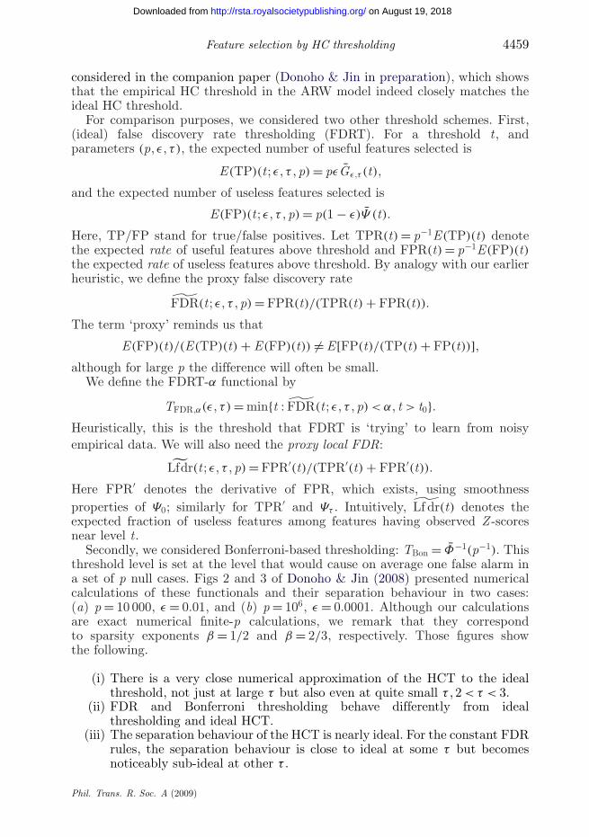
considered in the companion paper (Donoho & Jin in preparation), which showsthat the empirical HC threshold in the ARW model indeed closely matches theideal HC threshold.

For comparison purposes, we considered two other threshold schemes. First,(ideal) false discovery rate thresholding (FDRT). For a threshold t, andparameters (p, ε, τ), the expected number of useful features selected is

E(TP)(t; ε, τ , p) = pεGε,τ (t),

and the expected number of useless features selected is

E(FP)(t; ε, τ , p) = p(1 − ε)Ψ (t).

Here, TP/FP stand for true/false positives. Let TPR(t) = p−1E(TP)(t) denotethe expected rate of useful features above threshold and FPR(t) = p−1E(FP)(t)the expected rate of useless features above threshold. By analogy with our earlierheuristic, we define the proxy false discovery rate

˜FDR(t; ε, τ , p) = FPR(t)/(TPR(t) + FPR(t)).

The term ‘proxy’ reminds us that

E(FP)(t)/(E(TP)(t) + E(FP)(t)) = E[FP(t)/(TP(t) + FP(t))],although for large p the difference will often be small.

We define the FDRT-α functional by

TFDR,α(ε, τ) = min{t : ˜FDR(t; ε, τ , p) < α, t > t0}.Heuristically, this is the threshold that FDRT is ‘trying’ to learn from noisyempirical data. We will also need the proxy local FDR:

Lfdr(t; ε, τ , p) = FPR′(t)/(TPR′(t) + FPR′(t)).

Here FPR′ denotes the derivative of FPR, which exists, using smoothnessproperties of Ψ0; similarly for TPR′ and Ψτ . Intuitively, ˜Lf dr(t) denotes theexpected fraction of useless features among features having observed Z -scoresnear level t.

Secondly, we considered Bonferroni-based thresholding: TBon = Φ−1(p−1). Thisthreshold level is set at the level that would cause on average one false alarm ina set of p null cases. Figs 2 and 3 of Donoho & Jin (2008) presented numericalcalculations of these functionals and their separation behaviour in two cases:(a) p = 10 000, ε = 0.01, and (b) p = 106, ε = 0.0001. Although our calculationsare exact numerical finite-p calculations, we remark that they correspondto sparsity exponents β = 1/2 and β = 2/3, respectively. Those figures showthe following.

(i) There is a very close numerical approximation of the HCT to the idealthreshold, not just at large τ but also even at quite small τ , 2 < τ < 3.

(ii) FDR and Bonferroni thresholding behave differently from idealthresholding and ideal HCT.

(iii) The separation behaviour of the HCT is nearly ideal. For the constant FDRrules, the separation behaviour is close to ideal at some τ but becomesnoticeably sub-ideal at other τ .





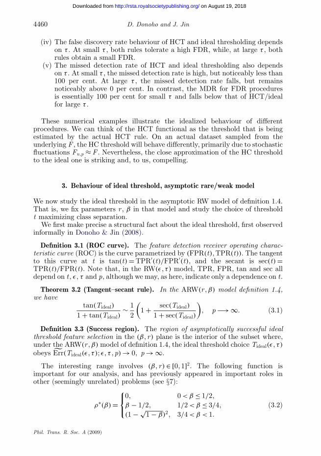
(iv) The false discovery rate behaviour of HCT and ideal thresholding dependson τ . At small τ , both rules tolerate a high FDR, while, at large τ , bothrules obtain a small FDR.

(v) The missed detection rate of HCT and ideal thresholding also dependson τ . At small τ , the missed detection rate is high, but noticeably less than100 per cent. At large τ , the missed detection rate falls, but remainsnoticeably above 0 per cent. In contrast, the MDR for FDR proceduresis essentially 100 per cent for small τ and falls below that of HCT/idealfor large τ .

These numerical examples illustrate the idealized behaviour of differentprocedures. We can think of the HCT functional as the threshold that is beingestimated by the actual HCT rule. On an actual dataset sampled from theunderlying F , the HC threshold will behave differently, primarily due to stochasticfluctuations Fn,p ≈ F . Nevertheless, the close approximation of the HC thresholdto the ideal one is striking and, to us, compelling.

3. Behaviour of ideal threshold, asymptotic rare/weak model

We now study the ideal threshold in the asymptotic RW model of definition 1.4.That is, we fix parameters r , β in that model and study the choice of thresholdt maximizing class separation.

We first make precise a structural fact about the ideal threshold, first observedinformally in Donoho & Jin (2008).

Definition 3.1 (ROC curve). The feature detection receiver operating charac-teristic curve (ROC) is the curve parametrized by (FPR(t), TPR(t)). The tangentto this curve at t is tan(t) = TPR′(t)/FPR′(t), and the secant is sec(t) =TPR(t)/FPR(t). Note that, in the RW(ε, τ) model, TPR, FPR, tan and sec alldepend on t, ε, τ and p, although we may, as here, indicate only a dependence on t.

Theorem 3.2 (Tangent–secant rule). In the ARW(r , β) model definition 1.4,we have

tan(Tideal)

1 + tan(Tideal)∼ 1

2

(1 + sec(Tideal)

1 + sec(Tideal)

), p −→ ∞. (3.1)

Definition 3.3 (Success region). The region of asymptotically successful idealthreshold feature selection in the (β, r) plane is the interior of the subset where,under the ARW(r , β) model of definition 1.4, the ideal threshold choice Tideal(ε, τ)

obeys Err(Tideal(ε, τ); ε, τ , p) → 0, p → ∞.

The interesting range involves (β, r) ∈ [0, 1]2. The following function isimportant for our analysis, and has previously appeared in important roles inother (seemingly unrelated) problems (see §7):

ρ∗(β) =⎧⎨⎩

0, 0 < β ≤ 1/2,β − 1/2, 1/2 < β ≤ 3/4,(1 − √

1 − β)2, 3/4 < β < 1.(3.2)





As it turns out, it marks the boundary between success and failure forthreshold feature selection. (The correct interpretation of ρ∗(β) = 0 for β ∈(0, 1/2] is simply that the critical value of τ separating success from failureis o(

√2 log p).)

Theorem 3.4 (Existence of phases). The success region is precisely r > ρ∗(β),0 < β < 1. In the interior of the complementary region, r < ρ∗(β), 1/2 < β < 1,even the ideal threshold cannot send the proxy separation to infinity withincreasing (n, p).

Definition 3.5 (Regions I, II, III). The success region can be split into threeregions, referred to here and below as regions I–III. The interiors of the regionsare as follows (figure 2):

I. 0 < r ≤ β/3 and 1/2 < β < 3/4; r > ρ∗(β).II. β/3 < r ≤ β and 1/2 < β < 1; r > ρ∗(β).

III. β < r < 1 and 1/2 < β < 1; r > ρ∗(β).

In the asymptotic RW model, the optimal threshold must behaveasymptotically like

√2q log p for a certain q = q(r , β). Surprisingly, we need not

have q = r .

Theorem 3.6 (Formula for ideal threshold). Under the asymptotic RWmodel ARW(r , β), with r > ρ∗(β), the ideal threshold has the form Tideal(ε, τ) ∼√

2q∗ log p where

q∗ ={4r , region I,(β + r)2/(4r), regions II, III.

(3.3)

Note in particular that, in regions I and II, q∗ > r , and hence Tideal(ε, τ) > τ .Although the features truly have strength τ , the threshold is best set higherthan τ . An apparently similar result was found in the detection setting (Donoho &Jin 2004), but the formula for q∗ was subtly different from equation (3.3).

We now turn to FDR properties. The tangent–secant rule implies immediately

˜Lf dr(Tideal)

(1 + ˜FDR(Tideal))/2−→ 1, p −→ ∞. (3.4)

Hence, any result about FDR is tied to one about local FDR, and vice versa.

Theorem 3.7. Under the asymptotic RW model ARW(r , β), at the idealthreshold Tideal(ε, τ), proxy FDR and proxy local FDR obey

˜FDR(Tideal, ε, τ) −→ b(β, r), ˜Lf dr(Tideal, ε, τ) −→ 1 + b(β, r)

2, p −→ ∞,

(3.5)where

b(β, r) =

⎧⎪⎪⎨⎪⎪⎩

1, region I,

(r + β)/(4r), region II (note β/3 < r < β),

1/2, region III.

Several aspects of the above solution are of interest.





(i) Threshold elevation. The threshold√

2q∗ log p is significantly higher than√2r log p in regions I and II. Instead of looking for features at the

amplitude they can be expected to have, we look for them at much higheramplitudes.

(ii) Fractional harvesting. Outside region III, we are selecting only a smallfraction of the truly useful features.

(iii) False discovery rate. Outside region III, we actually have a very large falsediscovery rate, which is very close to 1 in region I. Surprisingly, even thoughmost of the selected features are useless, we still correctly classify!

(iv) Training versus test performance. The quantity√

q can be interpretedas a ratio:

√q∗/r = max{(β + r)/2r , 2} = strength of useful features in

training/strength of those features in test. From equation (3.3), we learnthat, in region I, the selected useful features perform about half as well intesting as we might expect from their performance in training.

4. Behaviour of ideal clipping threshold

This section sketches the arguments supporting theorems 3.2, 3.4, 3.6 and 3.7.In view of space restrictions, arguments supporting lemmas from this and latersections may be found in the electronic supplementary material.

In the RW model, it makes particular sense to use the clipping thresholdfunction η

clipt , since all non-zeros are known to have the same amplitude. The

ideal clipping threshold is also very easy to analyse heuristically. However, itturns out that all the statements in theorems 3.2, 3.4, 3.6 and 3.7 are equallyvalid for all the three types of threshold function, so we prefer to explain thederivations using clipping.

(a) Sep in terms of true and false discoveries

In the RW model, we can express the components of the proxy separation verysimply when using the clipping threshold:

Aclip(t, ε, τ) = ετE[sgn(τ + W )1{|τ+W |>t}]and

Bclip(t, ε, τ) = εE[1{|τ+W |>t}] + (1 − ε)E[1{|W |>t}],where W denotes an N (0, 1) random variable. Recall the definitions of usefulselections TP and useless selections FP; we must also count inverted detections, forthe case where the μi > 0 but η

clipt (Zi) < 0. Put E(ID)(t; ε, τ , p) = εpΦ(−t − τ),

with Φ again the standard normal distribution, and define the inverted detectionrate by IDR = p−1E(ID). Then

Aclip(t; ε, τ) = τ(TPR(t) − 2IDR(t))

andBclip(t; ε, τ) = TPR(t) + FPR(t).

We arrive at an identity for Sep in the case of clipping:

Sep(t; ε, τ) = 2τ(TPR(t) − 2IDR(t))/√

TPR(t) + FPR(t).





To explain theorem 3.2, drop the term IDR and consider the alternative proxy

Sep(t) = (2τ)TPR(t)/√

TPR(t) + FPR(t) = 2A(t)/B1/2(t).

Lemma 4.1. Let ε > 0 and τ > 0. The threshold talt maximizing Sep(t) as afunction of t satisfies the tangent–secant rule as an exact identity; at this thresholdwe have Lf dr(talt) = 1

2(1 + FDR(talt)).

The connection Sep ∼ Sep follows from part (iii) of the next lemma.

(b) Analysis in the asymptotic rare/weak model

We now invoke the ARW(r , β) model: ε = p−β , τ = √2r log p, n ∼ c(log p)γ ,

p → ∞. Let tp(q) = √2q log p. We have

Ψ0(tp(q)) ∼√

2/πp−q

tp(q), p → ∞. (4.1)

We also need some notation for poly-log terms.Definition 4.2. Any occurrence of the symbol PL(p) denotes a term that falls

between C (log p)−ζ and C (log p)ζ as p → ∞ for some ζ > 0 and C > 0. Differentoccurrences of this symbol may stand for different such terms.

In particular, we may well have T1(p) = PL(p), T2(p) = PL(p), as p → ∞, andyet T1(p)/T2(p) → 1 as p → ∞. However, certainly T1(p)/T2(p) = PL(p), p → ∞.

The following lemma exposes the main phenomena driving theorems 3.2, 3.4,3.6 and 3.7. It follows by simple algebra, and several uses of Mills’ ratio (4.1) inthe convenient form Ψ0(tp(q)) = PL(p)p−β .

Lemma 4.3. In the asymptotic RW model, ARW(r , β), as p → ∞, we have thefollowing results.

(i) Quasi power law for useful feature discoveries:

E(TP)(tq(p), ε, τ) = PL(p)pδ(q,r ,β),

where the useful feature discovery exponent δ obeys

δ(q; β, r) ≡{1 − β, 0 < q ≤ r ,1 − β − (

√q − √

r)2, r < q < 1.

(ii) Quasi power law for useless feature discoveries:

E(FP)(tq(p), ε, τ) = PL(p)p1−q .(iii) Negligibility of inverted detections:

E(ID)(tq(p), ε, τ) = o(E(TP)(tq(p), ε, τ)).

As an immediate corollary, under ARW(r , β), we have

Sep(tq(p), ε, τ)(

12

√p/n

)= PL(p)pδ(q;β,r)/

√pδ(q;β,r) + p1−q , p → ∞.

On the right-hand side of this display, the poly-log term is relatively unimportant.The driving effect is the power-law behaviour of the fraction. The following lemmacontains the core idea behind the appearance of ρ∗ in theorems 3.2 and 3.4, andthe distinction between region I and regions II and III.





Lemma 4.4. Let (β, r) ∈ ( 12 , 1)2. For fixed q, r and β, let γ (q; r , β) denote the

rate at which pδ(q;β,r)/√

pδ(q;β,r) + p1−q tends to ∞ as p → ∞. Then γ > 0 if andonly if r > ρ∗(β). A choice of q maximizing this ratio is given by equation (3.3 ).

Lemma 4.4 shows that equation (3.3) gives us one choice of thresholdmaximizing the rate at which (

√p/n Sep) tends to infinity. Is it the only choice?

Define q2 = q2(r , β) = (β + r)2/(4r). Except in the case r > β (and so q2 ∈ (β, r)),this is indeed the only choice. As the proof of lemma 4.4 shows, if r > β,any q ∈ [β, r] optimizes the rate of separation. It turns out that, in that case,our formula q∗ not only maximizes the rate of separation, but also correctlydescribes the leading-order asymptotic behaviour of Tideal. The key point is thetangent–secant formula, which picks out, from among all q ∈ [β, r], uniquely q2.This is shown by the next two lemmas, which thereby complete the proof oftheorem 3.6.

Lemma 4.5. Set γ0(q; r , β) = −β − r + 2√

rq, for q ∈ (0, 1). In the ARW(r , β)model, consider the threshold tq(p). Then, as p → ∞,

TPR(tq(p))

FPR(tq(p))∼

⎧⎪⎪⎨⎪⎪⎩

pγ0(q,r ,β)

√q

2√

q − 2√

r, q > r ,

pq−β

√π

2tq(p), q < r .

(4.2)

Moreover, suppose q = r. Then

TPR′(tq(p))

FPR′(tq(p))= 1

2pγ0(q,r ,β), p → ∞. (4.3)

Lemma 4.6. The above defined q2(r , β) is the unique solution of γ0(q; r , β) = 0.Suppose r > β. As p → ∞, Tideal/tq2(p) → 1.

(c) False discovery rate/local false discovery rateproperties of ideal threshold

We now turn to Theorem 3.7 and make an important observation:

The asymptotic Tideal = tq∗(p)(1 + o(1)) is simply too crude todetermine the FDR and Lfdr properties of Tideal; it is necessaryto consider the second-order effects implicit in the (1 + o(1)) term.For this, the tangent–secant formula is essential.

Indeed, equation (4.3) shows that the only possibilities for limiting local FDRof a threshold of the exact form tq(p) are 0, 1/2, 1. The actual local FDR ofTideal spans a continuum from [0, 1], because small perturbations of tq(p)(1 + o(1))implicit in the o(1) can cause a change in the local FDR. To understand this, forq = r and s ∈ (0, ∞), put

q(q, r , s, p) =[r1/2 ±

√(q1/2 − r1/2)2 + (log s)/(log p)

]2,





where the sign of ± is + if and only if q > r . Clearly, q is well defined for allsufficiently large p. As an example, q(q, r , 1, p) = q. The peculiar definition ensuresthat φ(tq(p) − tr (p)) = φ(tq(p) − tr (p))s.

By simple algebra one can show the following result.

Lemma 4.7. Let q, r and s be fixed. With q = q(q, r , s, p), tq(p)/tq(p) → 1 andφ(tq(p))/φ(tq(p)) → 1, p → ∞.

Let us put for short Fs = FPR(tq(q,r ,s,p)(p)) and Ts = TPR(tq(q,r ,s,p)(p)).Combining several identities from the last few sentences, we have, as p → ∞,T ′

s = sT ′1, F ′

s ∼ F ′1, Ts ∼ sT1 and Fs ∼ F1. Hence,

FDR(tq(q,r ,s,p)(p)) = Fs/(Ts + Fs) ∼ F1/(sT1 + F1);

Lfdr(tq(q,r ,s,p)(p)) = F ′s/(T

′s + F ′

s) ∼ F ′1/(sT

′1 + F ′

1).

Choosing s appropriately, we can therefore obtain a perturbed q that perturbsthe Lfdr and FDR. In fact, there is a unique choice of s needed to ensure thetangent–secant formula.

Lemma 4.8. For given values F1, F ′1, T1 = 0 and T ′

1 = 0, put s∗ = (F ′1/T

′1) −

2(F1/T1). This choice of s obeys the tangent–secant rule: F ′1/(s

∗T ′1 + F ′

1) = 12(1 +

F1/(s∗T1 + F1)).

To use this, recall equations (4.2) and (4.3). These formulae give expressionsfor T1/F1 and T ′

1/F′1. Plugging in q = q∗, we get the following corollary.

Corollary 4.9. We have Tideal ∼ tq(q∗,r ,s∗,p)(p), where s∗ is obtained by settingT1 = (

√q∗ − √

r)−1, F1 = 2/√

q, T ′1 = 1 and F ′

1 = 2. Moreover, if β/3 < r < β,FDR(Tideal) ∼ (β − r)/2r, Lfdr(Tideal) ∼ (r + β)/4r.

5. Connection of higher criticism objective with ˜Sep

Let F = Fε,τ be the two-point mixture of definition 2.3 and G = Gε,τ thecorresponding folded distribution. For t = tq(p) in the asymptotic RW model,we have

HC(t; Fε,τ ) = G(t) − Ψ (t)√G(t)G(t)

= ε(Ψτ − Ψ0)(t)[((1 − ε)Ψ0 + εΨτ )((1 − ε)Ψ0 + εΨτ )]1/2

∼ ε(Ψτ − Ψ0)(t)[((1 − ε)Ψ0 + εΨτ )]1/2

∝ TPR(t) − ε/(1 − ε)FPR(t)[FPR(t) + TPR(t)]1/2

∼ TPR(t)[TPR(t) + FPR(t)]1/2

∼ (1 + o(1))Sep(t; ε, τ), p → ∞.

⎫⎪⎪⎪⎪⎪⎪⎪⎪⎪⎪⎪⎪⎪⎪⎪⎪⎪⎪⎪⎬⎪⎪⎪⎪⎪⎪⎪⎪⎪⎪⎪⎪⎪⎪⎪⎪⎪⎪⎪⎭

(5.1)





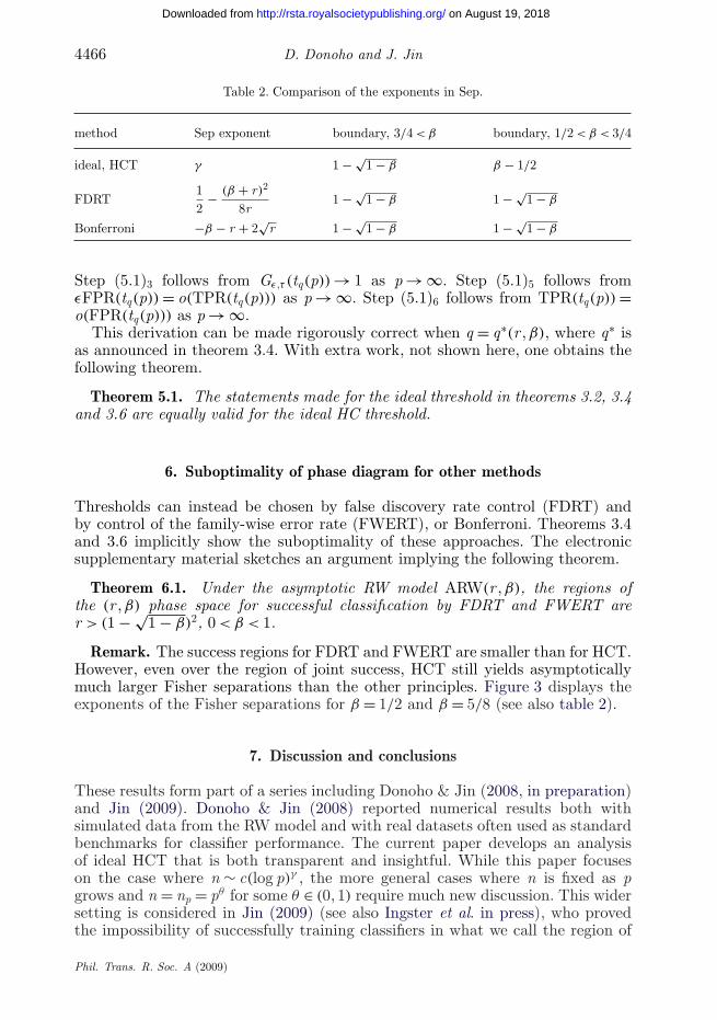
Table 2. Comparison of the exponents in Sep.

method Sep exponent boundary, 3/4 < β boundary, 1/2 < β < 3/4

ideal, HCT γ 1 − √1 − β β − 1/2

FDRT12

− (β + r)2

8r1 − √

1 − β 1 − √1 − β

Bonferroni −β − r + 2√

r 1 − √1 − β 1 − √

1 − β

Step (5.1)3 follows from Gε,τ (tq(p)) → 1 as p → ∞. Step (5.1)5 follows fromεFPR(tq(p)) = o(TPR(tq(p))) as p → ∞. Step (5.1)6 follows from TPR(tq(p)) =o(FPR(tq(p))) as p → ∞.

This derivation can be made rigorously correct when q = q∗(r , β), where q∗ isas announced in theorem 3.4. With extra work, not shown here, one obtains thefollowing theorem.

Theorem 5.1. The statements made for the ideal threshold in theorems 3.2, 3.4and 3.6 are equally valid for the ideal HC threshold.

6. Suboptimality of phase diagram for other methods

Thresholds can instead be chosen by false discovery rate control (FDRT) andby control of the family-wise error rate (FWERT), or Bonferroni. Theorems 3.4and 3.6 implicitly show the suboptimality of these approaches. The electronicsupplementary material sketches an argument implying the following theorem.

Theorem 6.1. Under the asymptotic RW model ARW(r , β), the regions ofthe (r , β) phase space for successful classification by FDRT and FWERT arer > (1 − √

1 − β)2, 0 < β < 1.

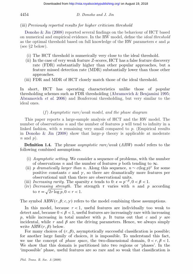
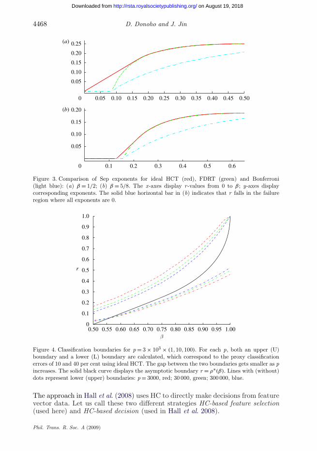
Remark. The success regions for FDRT and FWERT are smaller than for HCT.However, even over the region of joint success, HCT still yields asymptoticallymuch larger Fisher separations than the other principles. Figure 3 displays theexponents of the Fisher separations for β = 1/2 and β = 5/8 (see also table 2).

7. Discussion and conclusions

These results form part of a series including Donoho & Jin (2008, in preparation)and Jin (2009). Donoho & Jin (2008) reported numerical results both withsimulated data from the RW model and with real datasets often used as standardbenchmarks for classifier performance. The current paper develops an analysisof ideal HCT that is both transparent and insightful. While this paper focuseson the case where n ∼ c(log p)γ , the more general cases where n is fixed as pgrows and n = np = pθ for some θ ∈ (0, 1) require much new discussion. This widersetting is considered in Jin (2009) (see also Ingster et al. in press), who provedthe impossibility of successfully training classifiers in what we call the region of





impossibility. In Donoho & Jin (in preparation), we will develop a complete setof results for the more general linkages of n with p and for HCT as opposed toideal HCT.

Beyond ideal performance. Conceptually, the ideal threshold envisages asituation with an oracle, who, knowing ε and τ , and n and p, chooses the very bestthreshold possible under those given parameters. In this paper we have analysedthe behaviour of this threshold within a certain asymptotic framework. Clearly,no empirical procedure can duplicate the performance of the ideal threshold.

However, HC thresholding comes close. The HC threshold does not involveoptimal exploitation of knowledge of ε and τ ; it needs only the feature Z -scores.In this paper, we analysed the behaviour of the ideal HCT: tHC = THC(Fε,τ ).

This is an ideal procedure because in a real-life situation we do not knowthe distribution Fε,τ of Z -scores; we have instead the empirical cumulativedistribution function (CDF) Fn,p defined by Fn,p(z) = (1/p)

∑pj=1 1{Z ( j)≤z}. The

(non-ideal) HCT that we defined in §1e is then simply tHCn,p = THC(Fn,p). Because

Fε,τ (z) = E(Fn,p)(z), there is nothing controversial about the assertion thattHC ≈ tHC

n,p for large n and p. Indeed, there are generations of experience forother functionals T showing that we typically have T (Fn,p) ≈ T (E(Fn,p)) forlarge n, p for those other functionals. Proving this for T = THC is morechallenging than one might anticipate; the problem is that the functionalTHC is not continuous at F = Φ, and yet Fε(p),τ(p) → Φ as p → ∞. Afterconsiderable effort, we justify the approximation of HCT by ideal HCT inDonoho & Jin (in preparation). The analysis presented here only partiallyproves that HCT gives near-optimal threshold feature selection; it onlyexplains the connection at the level of ideal quantities. But this is themain insight.

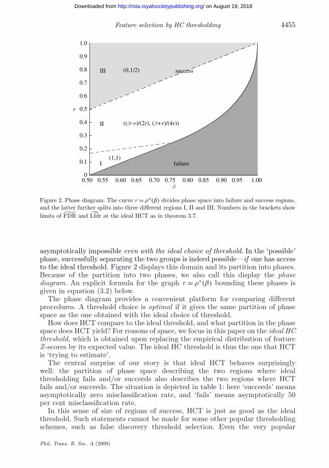
Phase diagram for finite sample sizes. The phase diagram correctly reflectsfinite (n, p) behaviour. In figure 4, we consider p = 3 × 103 × N , N = (1, 10, 100).For such p, we take n = (log p)/2 and display the boundary of the set of(β, r), where ideal HCT yields a classification error between 10 and 40per cent. As p grows, the upper and lower bounds migrate towards the limitcurve r = ρ∗(β).

Other work on HC. HC was originally proposed for use in a detection problemthat has nothing to do with threshold feature selection: testing an intersectionnull hypothesis μ( j) = 0, for all j (Donoho & Jin 2004). The literature hasdeveloped since then. Hall & Jin (2008, 2009) extend the optimality of HC indetection to correlated settings. Wellner and his collaborators investigated HC inthe context of goodness of fit; see for example Jager & Wellner (2007). Hall andhis collaborators have investigated HC for robustness; see for example Delaigle &Hall (2009). HC has been applied to data analysis in cosmology and astronomy(Cayon et al. 2005; Jin et al. 2005). HC has also been used as a principle tosynthesize new procedures: Cai et al. (2007) use HC to motivate estimators forthe proportion ε of non-null effects.

HC in classification. HC was previously applied to high-dimensionalclassification in Hall et al. (2008), but with a key conceptual difference fromthe present paper. Our approach uses HC in classifier training—it selectsfeatures in designing a linear classifier—but the actual classification decisionsare made by the linear classifier when presented with specific test feature vectors.





0 0.05 0.10 0.15 0.20 0.25 0.30 0.35 0.40 0.45 0.50

0.05

0.10

0.15

0.20

0.25

0.1 0.2 0.3 0.4 0.5 0.60

0.05

0.10

0.15

0.20

(a)

(b)

Figure 3. Comparison of Sep exponents for ideal HCT (red), FDRT (green) and Bonferroni(light blue): (a) β = 1/2; (b) β = 5/8. The x-axes display r-values from 0 to β; y-axes displaycorresponding exponents. The solid blue horizontal bar in (b) indicates that r falls in the failureregion where all exponents are 0.

0.50 0.55 0.60 0.65 0.70 0.75 0.80 0.85 0.90 0.95 1.000

0.1

0.2

0.3

0.4

0.5

0.6

0.7

0.8

0.9

1.0

β

r

Figure 4. Classification boundaries for p = 3 × 103 × (1, 10, 100). For each p, both an upper (U)boundary and a lower (L) boundary are calculated, which correspond to the proxy classificationerrors of 10 and 40 per cent using ideal HCT. The gap between the two boundaries gets smaller as pincreases. The solid black curve displays the asymptotic boundary r = ρ∗(β). Lines with (without)dots represent lower (upper) boundaries: p = 3000, red; 30 000, green; 300 000, blue.

The approach in Hall et al. (2008) uses HC to directly make decisions from featurevector data. Let us call these two different strategies HC-based feature selection(used here) and HC-based decision (used in Hall et al. 2008).





In the ARW model, for a given classifier performance level, the HC-baseddecision strategy requires much stronger feature contrasts to reach that levelthan the HC-based feature selection strategy. In this paper, we have shownthat HC feature selection requires useful features to have contrasts exceeding√

2ρ∗(β) log p/√

n(1 + o(1)), (n, p) → ∞. HC decision requires useful featuresto have contrasts exceeding

√2ρ∗(β) log p(1 + o(1)), p → ∞. Therefore, if the

number of training samples n > 1, HC feature selection has an advantage. Imaginethat we have n = 36 training samples; we will find that HC feature selection canasymptotically detect features at roughly 1/6 the strength required when usingHC directly for decision.

Other work on the RW model. During the review of this paper, a newmanuscript by Ingster et al. (2009) appeared in arXiv analysing a feature selectionsetting equivalent to the ARW model, using non-HC-based approaches.

The authors would like to thank the Isaac Newton Mathematical Institute at Cambridge forhospitality during the program Statistical Theory and Methods for Complex, High-DimensionalData, and for a Rothschild Visiting Professorship held by D.D. We would also like to thankan anonymous referee for many helpful comments. D.D. was partially supported by NSFDMS-0505303, and J.J. was partially supported by NSF CAREER award DMS-0908613.

References

Abramovich, F. & Benjamini, Y. 1995 Thresholding of wavelet coefficients as multiple hypothesestesting procedure. In Wavelets and statistics (eds A. Antoniadis & G. Oppenheim), pp. 5–14.New York, NY: Springer.

Abramovich, F., Benjamini, Y., Donoho, D. & Johnstone, I. 2006 Adapting to unknown sparsity bycontrolling the false discovery rate. Ann. Stat. 34, 584–653. (doi:10.1214/009053606000000074)

Anderson, T. W. 2003 An introduction to multivariate statistical analysis, 3rd edn. New York, NY:Wiley.

Benjamini, Y. & Hochberg, Y. 1995 Controlling the false discovery rate: a practical and powerfulapproach to multiple testing. J. R. Stat. Soc. B 57, 289–300.

Bickel, P. & Levina, E. 2004 Some theory of Fisher’s linear discriminant function, ‘naive Bayes’,and some alternatives when there are many more variables than observations. Bernoulli 10,989–1010. (doi:10.3150/bj/110631487)

Cai, T., Jin, J. & Low, M. 2007 Estimation and confidence sets for sparse normal mixtures. Ann.Stat. 35, 2421–2449. (doi:10.1214/009053607000000334)

Cayon, L., Jin, J. & Treaster, A. 2005 Higher criticism statistic: detecting and identifyingnon-Gaussianity in the WMAP first year data. Mon. Not. R. Astron. Soc. 362, 826–832.(doi:10.1111/j.1365-2966.2005.09277.x)

Delaigle, A. & Hall, J. 2009 Higher criticism in the context of unknown distribution, non-independence and classification. In Perspectives in mathematical sciences I: Probability andstatistics, Platinum Jubilee Proceedings of the Indian Statistical Institute (eds N. S. NarasimhaSastry, T. S. S. R. K. Rao, M. Delampady & B. Rajeev), Statistical Science and InterdisciplinaryResearch, vol. 7, pp. 109–138. Hackensack, NJ: World Scientific.

Donoho, D. & Jin, J. 2004 Higher criticism for detecting sparse heterogeneous mixtures. Ann. Stat.32, 962–994. (doi:10.1214/009053604000000265)

Donoho, D. & Jin, J. 2006 Asymptotic minimaxity of false discovery rate thresholding for sparseexponential data. Ann. Stat. 34, 2980–3018. (doi:10.1214/009053606000000920)

Donoho, D. & Jin, J. 2008 Higher criticism thresholding: optimal feature selection when usefulfeatures are rare and weak. Proc. Natl Acad. Sci. USA 105, 14 790–14 795. (doi:10.1073/pnas.0807471105)

Donoho, D. & Jin, J. In preparation. If useful features are rare and weak, HCT yields successfulclassification where success is possible.


http://dx.doi.org/doi:10.1214/009053606000000074

http://dx.doi.org/doi:10.3150/bj/110631487


http://dx.doi.org/doi:10.1111/j.1365-2966.2005.09277.x



http://dx.doi.org/doi:10.1073/pnas.0807471105





Donoho, D. & Johnstone, I. 1994 Minimax risk over lp-balls for lq -error. Prob. Theory RelatedFields 2, 277–303.

Donoho, D., Johnstone, I., Hoch, J. C. & Stern, A. S. 1992 Maximum entropy and the nearly blackobject. J. R. Stat. Soc. B 54, 41–81.

Efron, B., Tibshirani, R., Storey, J. & Tusher, V. 2001 Empirical Bayes analysis of a microarrayexperiment. J. Am. Stat. Assoc. 99, 96–104. (doi:10.1198/016214504000000089)

Fan, J. & Fan, Y. 2008 High-dimensional classification using features annealed independence rules.Ann. Stat. 36, 2605–2637. (doi:10.1214/07-AOS504)

Golub, T. et al. (1999) Molecular classification of cancer: class discovery and classprediction by gene expression monitoring. Science 286, 531–536. (doi:10.1126/science.286.5439.531)

Hall, P. & Jin, J. 2008 Properties of higher criticism under strong dependence. Ann. Stat. 36,381–402. (doi:10.1214/009053607000000767)

Hall, P. & Jin, J. 2009 Innovative higher criticism for detecting sparse signals in correlated noise.(http://arxiv.org/abs/0902.3837v1).

Hall, P., Pittelkow, Y. & Ghosh, M. 2008 Theoretical measures of relative performance ofclassifiers for high dimensional data with small sample sizes. J. R. Stat. Soc. B 70,158–173.

Hedenfalk, I. et al. 2001 Gene-expression profile in hereditary breast cancer. N. Engl. J. Med. 344,539–448. (doi:10.1056/NEJM200102223440801)

Ingster, Yu. I. 1997 Some problems of hypothesis testing leading to infinitely divisible distribution.Math. Methods Stat. 6, 47–69.

Ingster, Yu. I., Pouet, C. & Tsybakov, A. B. 2009 Sparse classification boundaries.(http://arxiv.org/abs/0903.4807v1).

Ingster, Yu. I., Pouet, C. & Tsybakov, A. B. 2009 Classification of sparse high-dimensional vectors.Phil. Trans. R. Soc. A 367, 4427–4448. (doi:10.1098/rsta.2009.0156)

Jager, L. & Wellner, J. 2007 Goodness-of-fit tests via phi-divergences. Ann. Stat. 35, 2018–2053.(doi:10.1214/0009053607000000244)

Jin, J. 2003 Detecting and estimating sparse mixtures. PhD thesis, Department of Statistics,Stanford University.

Jin, J. 2009 Impossibility of successful classification when useful features are rare and weak. Proc.Natl Acad. Sci. USA 106, 8859–8864. (doi:10.1073/pnas.0903931106)

Jin, J., Starck, J.-L., Donoho, D., Aghanim, N. & Forni, O. 2005 Cosmological non-Gaussiansignature detection: comparing performances of different statistical tests. EURASIP J. Appl.Signal Process 15, 2470–2485. (doi:10.1155/ASP.2005.2470)

Johnstone, I. & Silverman, B. 2004 Needles and straw in haystacks: empirical Bayes estimates ofpossibly sparse sequences. Ann. Stat. 32, 1594–1649. (doi:10.1214/009053604000000030)

Tibshirani, R., Hastie, T., Narasimhan, B. & Chu, G. 2002 Diagnosis of multiple cancer types byshrunken centroids of gene expression. Proc. Natl Acad. Sci. USA 99, 6567–6572. (doi:10.1073/pnas.082099299)



http://dx.doi.org/doi:10.1214/07-AOS504

http://dx.doi.org/doi:10.1126/science.286.5439.531

http://dx.doi.org/doi:10.1126/science.286.5439.531


http://arxiv.org/abs/0902.3837v1

http://dx.doi.org/doi:10.1056/NEJM200102223440801

http://arxiv.org/abs/0903.4807v1

http://dx.doi.org/doi:10.1098/rsta.2009.0156



http://dx.doi.org/doi:10.1155/ASP.2005.2470





Feature selection by higher criticism thresholding...

Documents

Transcript of Feature selection by higher criticism thresholding...