Feature-Based Visual Sentiment Analysis of Text Document Streams

CHRISTIAN ROHRDANTZ, University of Konstanz

MING C. HAO, UMESHWAR DAYAL, and LARS-ERIK HAUG, Hewlett Packard Labs

DANIEL A. KEIM, University of Konstanz

This article describes automatic methods and interactive visualizations that are tightly coupled with the

goal to enable users to detect interesting portions of text document streams. In this scenario the inter-

estingness is derived from the sentiment, temporal density, and context coherence that comments about

features for different targets (e.g., persons, institutions, product attributes, topics, etc.) have. Contribu-

tions are made at different stages of the visual analytics pipeline, including novel ways to visualize salient

temporal accumulations for further exploration. Moreover, based on the visualization, an automatic algo-

rithm aims to detect and preselect interesting time interval patterns for different features in order to guide

analysts. The main target group for the suggested methods are business analysts who want to explore

time-stamped customer feedback to detect critical issues. Finally, application case studies on two different

datasets and scenarios are conducted and an extensive evaluation is provided for the presented intelligent

visual interface for feature-based sentiment exploration over time.

Categories and Subject Descriptors: H.1.2 [Models and Principles]: User/Machine Systems—Human

information processing; H.3.1 [Information Storage and Retrieval]: Content Analysis and Indexing—

Linguistic processing; H.5.2 [Information Interfaces and Presentation]: User Interfaces—Graphical

user interfaces; H.4.0 [Information Systems Applications]: General; I.2.7 [Artificial Intelligence]:

Natural Language Processing—Text analysis; I.3.6 [Computer Graphics]: Methodology and Techniques—

Interaction Techniques; I.7.5 [Document and Text Processing]: Document Capture—Document analysis;

I.5.4 [Pattern Recognition]: Applications—Text processing; I.5.5 [Pattern Recognition]: Implementa-

tion—Interactive systems; J.1 [Administrative Data Processing]: Business

General Terms: Algorithms, Design, Human Factors

Additional Key Words and Phrases: Document time series, sentiment analysis, text mining, visual analytics

1. INTRODUCTION

In the last decade the amount of textual information readily available in digitalform has increased enormously. Especially, the amount of user-generated contenthas grown at a fast pace lately, as the Web 2.0 has enabled easy participation for all

Authors’ addresses: C. Rohrdantz (corresponding author), University of Konstanz, Box 78, 78457 Konstanz,Germany; email: christian.rohrdantz@uni-konstanz.de; M. C. Hao, U. Dayal, and L.-E. Haug, HewlettPackard Labs, 1501 Page Mill Road, Palo Alto, CA 94304; D. A. Keim, University of Konstanz, Box 78,78457 Konstanz, Germany.Permission to make digital or hard copies of part or all of this work for personal or classroom use is grantedwithout fee provided that copies are not made or distributed for profit or commercial advantage and thatcopies show this notice on the first page or initial screen of a display along with the full citation. Copyrightsfor components of this work owned by others than ACM must be honored. Abstracting with credit is permit-ted. To copy otherwise, to republish, to post on servers, to redistribute to lists, or to use any component ofthis work in other works requires prior specific permission and/or a fee. Permissions may be requested fromthe Publications Dept., ACM, Inc., 2 Penn Plaza, Suite 701, New York, NY 10121-0701, USA, fax +1 (212)869-0481, or permissions@acm.org.

2

Internet users. Large amounts of texts are provided through blogs, forums, wikis,twitter messages, companies’ online surveys, and feedback forms and also throughmore formal publications like RSS news feeds and online news Web sites.

These text sources constitute a rich body of information that is valuable to exploitfor different stakeholders with different information needs. Methods from text mining,natural language processing, and computational linguistics can help to extract inter-esting features out of the raw text data. However, not only automatic algorithms fordata analysis are important, but also to appropriately convey detected peculiaritiesto the analyst and offer possibilities for interactive data exploration. In the case ofsuch complex and ambiguous data as natural language text this requires possibilitiesto drill-down to the original text sources whenever needed in order to make sense ofthe automatic analysis, to enable an easy visual detection of interesting patterns, andto provide means to quickly generate or verify hypotheses. Methods from the fieldsof visual analytics and information visualization have been demonstrably shown tosupport such tasks.

In many concrete text analysis scenarios one crucial requirement is to extractsentiments or opinions contained in the documents. For example, companies mightbe interested in what their customers like or dislike about their products and ser-vices respectively what sentiments are associated with the brand or its productsin news. Similarly, organizations or individuals of public interest have to be awareof what is reported about them in news and how their decisions and statementsare reflected. Of course, many more related examples can be found, where opinionsor sentiments on certain topics have a high relevance. The vibrant field of opin-ion and sentiment analysis is dedicated to detect these kinds of statements fromtext.

As Web communication and publishing happens in real time more and more, a fur-ther particularly interesting issue from the data analysis perspective is the involve-ment of the time dimension. Temporal aspects like the distribution of text featuresover time and potentially also analyses in real time can be critical in different real-world applications.

This article is devoted to integrating methods from text mining, sentiment analysis,and visual analytics to enable the analyst to detect interesting temporal sentimentpatterns in text document streams. The main target group for the suggested meth-ods are business analysts that want to perform a temporal analysis of feedback thatcustomers directly send to a company via Web surveys.

For this purpose sentiments are extracted for features of different targets appearingin a text (e.g., products, persons, topics, etc.). In a next step, interactive visualizationsare introduced that provide global temporal overview or allow detailed insights intotemporal sentiment patterns about features. Furthermore, an automatic algorithmwas designed that detects interesting sentiment patterns with a high temporal den-sity and content coherence to guide the expert during analysis. Figure 1 gives anillustrating example.

Finally, application case studies are provided for two different analysis scenarioson document streams with different characteristics and an extensive evaluation isprovided.

2. RELATED WORK

This section describes relevant related work on automatic and visual feature-based sentiment analysis (Section 2.1), and the visual analysis of text time series(Section 2.2).

3

Fig. 1. Time density plots of an issue on the feature "password" with associated terms (bottom) and auto­matically annotated example comments (top). Among 50,000 customer comments, received within two years, all those are sequentially displayed that contain the noun "password". Each comment is represented by one vertic·al bar. The color indicates whether the noun "password" has been mentioned in a positive (green), negative (red), or neutral (gray) context. The height of a bar can encode another data dimension. In this case we experimented with the uncertainty involved in the sentiment analysis: the lower the bar, the more uncertain. The curve plotted below the sequential sentiment track is a time density track: the curve is high if the comments above have been relatively close in time. An automatic algorithm detects and highlights interesting portions of the visualization that analysts should explore in detail. Mousing over single com­ments, the content is displayed and the coloring of words indicates what the sentiment analysis has found. All nouns get a background coloring according to their sentiment context, sentiment words get font colors, and negation words are printed in italics. If the sentiment analysis of a noun was evaluated to be confident (little uncertainty) the corresponding word is underlined. Here, this is the case for "order" and "sales rep".

2.1. Feature-Based Sentiment Analysis

Feature-based sentiment analysis is a subtask of opinion and sentiment analysis. In literature the terms opinion and sentiment are often used interchangeably. For sim­plicity, in our approach we will use the term sentiment only.

Most approaches for feature-based sentiment analysis involve three or four consec­utive steps.

(1) Features for different targets (e.g., persons, organizations, products, services, or topics) are detected either directly from the corpus or based on predefined word lists.

(2) Sentiment words that describe the extracted features are searched in the docu­ments. Sentiment words are words that evoke positive or negative associations.

(3) A mapping strategy aims to detect which sentiment words refer to which feature, so that a sentiment score can be determined for each feature.

(4) Some approaches visualize the results of the feature-based sentiment analysis and enable the user to interactively explore the results in detail.

For the first two steps aht.mdant research has been published in the last years. For the sake ofbrevity we refer to comprehensive summaries given in Pang and Lee [2008] and Liu [2010] for details. Both features and sentiment words can be either learned from the processed text documents themselves, from external resources (e.g. , WordNet1) ,

or they can be gathered from predefined lists. One special challenge is to identify sentiment words that have no general validity, but depend on the domain or even on the feature. For example, in a domain like "printer" an adjective like "fast" is feature dependent, that is, positive in the sentence "the printer prints fast" and negative in the sentence "the ink cartridge runs out fast."

Details about steps 3 and 4 are listed in Sections 2 .1.1 and 2.1.2.

1 http://wordnet.princeton.edu/

4

2.1.1. Sentiment-to-Feature Mapping. Different approaches have been suggested in thepast to determine which sentiment words refer to which feature. Some of them usedistance-based heuristics, that is, the closer a sentiment word is to a feature word,the higher is its sentiment influence on the feature. Such approaches operate on wholesentences [Ding et al. 2008], on sentence segments ([Ding and Liu 2007; Kim and Hovy2004], or predefined word windows [Oelke et al. 2009].

Other approaches exploit advanced natural language processing methods, liketyped-dependency parsers, to resolve linguistic references from sentiment words tofeatures. There are several methods that resolve such references and thus can be usedfor feature-based sentiment analysis, although most of them were created for differentpurposes. Ng et al. [2006] use subject-verb, verb-object, and adjective-noun relationsfor polarity classification. Qiu et al. [2009] use dependency relations to extract bothfeatures (product attributes) and sentiment adjectives from reviews by a double prop-agation method. Popescu and Etzioni [2005] extract pairs (sentiment word, feature)based on 10 extraction rules that work on dependency relations and Riloff and Wiebe[2003] use lexico-syntactic patterns in a bootstrapping approach for subjectivity clas-sification resolving relations between opinion holders and verbs. Our method differsfrom the previous ones in that we use a predefined set of syntactic reference patternsthat are based on part-of-speech sequences only, in order to resolve references, insteadof using typed dependencies. In cases where this linguistically motivated method isnot able to resolve references, we rely on a distance-based heuristic. This approachalso allows us to estimate a degree of uncertainty involved in the analysis.

Recently, another approach was published that takes uncertainty into account [Wuet al. 2010]. The authors consider if customers do not express clear opinions, that is,“customers’ conflict and uncertainty about their opinions” as well as the uncertaintyinvolved in the automatic opinion analysis processing. As a result a feature mentioncan be both negative and positive at the same time. Their uncertainty score is basedon two parameters: The smaller the difference between the negative and positive sen-timent on a feature within a sentence and the longer the sentence, the higher theuncertainty. We also capture uncertainty in our analysis, however, we limit the analy-sis to the uncertainty the algorithm has when evaluating a sentence. In contrast to theexisting approach, our method relies on linguistic knowledge and not only on distance-based heuristics. In addition, the sentence length is not relevant in our analysis as weconsider only sentence segments.

2.1.2. Visual Exploration of Feature-Based Sentiment Analyses. Several different ap-proaches have been suggested to visualize the outcome of automatic feature-based sen-timent analyses and enable further user explorations. The Opinion Observer [Liu et al.2005] visualization enables users to compare products with respect to the amount ofpositive and negative reviews on different product features. A more scalable approachfor the same purpose, that is able to display more products and features at once, isthat of the Summary Reports presented in Oelke et al. [2009]. The same paper pro-vides further visualizations to identify groups of customers with similar opinions andcorrelations between individual feature scores and overall ratings. The AMAZINGSystem [Miao et al. 2009] also visualizes the sentiment of product reviews on certainproducts over time. The number of positive and negative reviews are aggregated overmonths and displayed with line charts. In Wanner et al. [2009] a visualization is sug-gested to track sentiments expressed in RSS news feeds on political parties and theircandidates during a presidential election.

Recently, OpinionSeer [Wu et al. 2010], a novel visual analysis tool for hotel reviews,was introduced, where uncertainty contained in reviews is visually represented andaggregated analyses can be performed, for example, on day, week, and month scale.

5

In contrast to the previous work, our approach enables a much more detailed insightinto the temporal development of sentiments on individual features.

2.2. Visual Text Time-Series Analysis

A comprehensive survey about the visualization and visual analysis of time series isgiven in Aigner et al. [2007]. Several further publications on the visual explorationof time-series data are related to the TimeSearcher Project2. Methods especially de-signed for text time series are often based on a linearly scaled time line, aggregatingevents according to predefined time bins. Many of these approaches have been inspiredby the ThemeRiver method [Havre et al. 2002]. So-called History Flows are used byViegas et al. [2004] to track collaborative authoring. Krstajic et al. [2010] visualizedaily aggregates of entity occurrences in news with stacked time series.

One particularity of our approach, however, is that it deals with unevenly spaceddata streams in which events (here: feature occurrences) may occur with an arbitrar-ily skewed temporal distribution. That means that the data includes short time spanswith high amounts of incoming data and large time spans that are only sparsely popu-lated. In Aris et al. [2005] several methods are presented to deal with unevenly spacedauction data. The (interleaved) event index method is the most similar one to our timedensity plots. It distorts the time axis in order to grant the same amount of space toeach event. While the temporal order is preserved the exact temporal relations arelost. Since the exact time between two consecutive events is not conveyed, the authorstry to support the user by shading the time axis segments.

Our visualization complements the previous work, in that it displays data recordsin sequential order without overlap and empty space, while still conveying informationabout exact temporal relations.

3. OUR APPROACH

Most of the previously mentioned feature-based sentiment analysis approaches dealwith collections of customer reviews on a certain product, as can be found on retailersides such as amazon.com. In contrast, this article focuses on customer reviews thatare directly sent to a company via a Web survey. This direct feedback is not necessarilyrelated to products but refers to any issue within the purchase and service process.Most importantly, not only the sentiment polarity but also the temporal and contextcoherence of customer comments are considered to detect critical issues that occur atcertain points in time. This paper covers the whole pipeline of methods necessaryto detect important sentiment pattern information in large document streams andcontributes at different stages of the analysis process by suggesting novel automaticand visual analysis approaches; see Figure 2. The required input for our analysisis rather generic in order to guarantee a wide applicability. It consists of a set oftime-stamped texts. To give an overview of the analysis steps, they are listed in thefollowing. Contributions are briefly explained.

— Linguistic Preprocessing— Feature Sentiment Identification. In the sentiment-to-feature attribution we aim to

achieve a good coverage while being as accurate as possible. Therefore, we combinedifferent methods to resolve sentiment-to-feature references and together with theanalysis results we give an estimation for the uncertainty involved in the analysis.This is a minor contribution that is not central to the overall approach but wasconsidered interesting to explore. For details see Section 4.

— Context Identification

2http://www.cs.umd.edu/hcil/timesearcher/

6

VfJu.llluUon and Jntll!!ractive V1w.al Analysis

Fig. 2. Overview of the steps involved in the visual analysis.

- Feature Time Density Calculation. Along the temporal dimension, we try to detect shifts in the occurrence frequency of a certain feature which may indicate time­related issues. The time density is calculated relative to the overall occurrence frequency of the feature. This allows us to detect interesting time patterns also for infrequent features. For details see Section 5.2.

- Visualization and Interactive Visual Analysis. To visualize sudden temporal ac­cumulations of comments on one feature, we propose an innovative visualization method: Sequential sentiment tracks together with time density tracks are able to display unevenly distributed feature occurrences without overlap and space­consuming gaps. Critical issues can readily be detected visually and explored in detail interactively accessing the relevant full text as a tooltip, as shown in Figure 1. To provide a global overview about the data distribution, pixel map calenders are applied. For details see Section 5.

- Time Interval Pattern Detection. In order to guide an analyst and advise her/him of critical issues, we further propose a new time pattern detection algorithm that operates both on past data and is also applicable in real time. Interesting time spans for features will be filtered and ranked according to their importance scores providing the basis for triggering real-time alerts. Patterns have to be comparatively dense in time, with a smooth time density curve, have to have a clearly negative sentiment connotation, and the feature has to appear in similar contexts within the documents of the pattern. With the purpose to determine the context coherence, terms are extracted that have a strong association with the pattern. Patterns are highlighted in the visualization and the associated terms are displayed in order to provide a quick insight. For details see Section 6.

To the best of our knowledge there are no other comparable approaches that offer a complete pipeline for the visual analysis of time-dependent sentiment patterns for text features. In Section 3 we discuss characteristics of two different datasets we use. Section 4 gives details about the feature-based sentiment analysis, Section 5 explains the visual analysis components, and Section 6 details the detection of interesting time interval patterns. In Section 7 we provide application case studies discussing

7

interesting results that were obtained on real data. An extensive evaluation ofdifferent parts of our approach including an expert user study is given in Section 8,where also advantages and limitations are discussed. In Section 9, we conclude thearticle with a summary.

Data and Applications

Our target users are industries, companies, and small businesses who want to exploretheir customer feedback. In addition to Web surveys, we also can readily apply ourvisualization and pattern detection methods to time-stamped news, twitter data, hotelreviews, movie/recreations reviews, etc., as long as the quality of the sentiment anal-ysis in that domain is reasonable. We use mostly standard methods for the automaticsentiment analysis that were suggested for mining customer reviews.

To apply our methods to datasets with different analysis scenarios and characteris-tics, in addition to customer Web surveys also RSS news feeds were explored.

— Customer Web Surveys. Web surveys give users the opportunity to directly com-ment, in a detailed way, on issues they liked or disliked about the product itselfand its purchase, service, delivery, payments, etc. This kind of information can beespecially valuable for companies as it might point them to problems that they hadbeen unaware of beforehand, having negative effects on their business performanceif the problems are not detected and eliminated in time. We gathered a datasetcontaining about 50,000 Web survey responses sent to a company between 2007and 2009.

— RSS News Feeds. RSS news feeds redistribute and spread current news in real time.For example, they are interesting for political analysts who want to see when andwhy political parties and persons are mentioned in negative contexts. To explorethe applicability of our methods for such a related task, we analyzed about 16,000RSS news items collected from 50 feeds about the U.S. presidential election in 2008.The collection started about one month before the election and ended on the electionday. The dataset was also used in Wanner et al. [2009].

4. FEATURE-BASED SENTIMENT ANALYSIS IN DOCUMENT STREAMS

The kind of data we deal with does not have a predefined limited topic coverage. Thereis no fixed set of features, that is, we are interested in any kind of feature for any kindof target (persons, organizations, products, services, topics, etc.). This also impliesthat we cannot define a domain- or attribute-dependent sentiment word list, but haveto rely on sentiment words with general validity. The feature-based sentiment analysiscomprises several steps where we apply standard methods.

(1) Linguistic Preprocessing. In a preprocessing step we apply part-of-speech tagging3

and lemmatization. Next, predefined negation words and their scope are detectedin sentences. Later, the polarity of sentiment words occurring after negations isinverted. The negation remains valid in the same sentence until one of the wordsor punctuation marks typically marking the end of a negation frame is encountered(e.g., ”,”, ”-”, ”but”, ”and”, ”though”, ”however”, etc.).

(2) Feature Extraction. All nouns and compound nouns are extracted as candidatefeatures. Whether a feature is interesting or not will only be determined in thelater time-related analysis. Features and further content-bearing context words

3http://opennlp.sourceforge.net/

8

Legend: =wildcard

NN=Noun JJ =Adjective RB = Adverb VB=Verb DT = Determiner Fealure Referencing Sentiment :'lloSenHment

Fig. 3. Syntactic sentiment reference patterns. Word order patterns go from left to right, the level indicates the exact position. The first pattern at the top left, for example, would match a sentence like " IIPRP really/RB like/VBP thisfDT printer INN". The positive polarity of the verb "to like" would then be attributed to the noun "printer". The graph summarizes the most frequent reliable patterns we could detect in our data and we therefore regarded in the analysis. In total, the graph covers 18 different patterns, one for each blue node.

(verbs and adjectives) are saved together with the information whether they ap­peared in a negated context. The context words are used when evaluating context coherences of interesting feature time interval patterns (see Section 6).

(3) Sentiment Word Detection. The polarity categories (positive, negative) from the Internet General Inquirer4 are applied in order to find sentiment words. The lists have been manually enhanced by removing some arguable words and adding fur­ther colloquial words. The positive word list contained 1594 words after removing 40 and adding 90. The negative word list contained 2018 words after removing 14 and adding 138.

(4) Sentiment-to-Feature Mapping. While the processing steps 1-3 are very similar to what has been done by other approaches before, this step includes novelties in that it relies both on syntactic Teference patterns and distance-based heuristics. It is described in detail in Section 4.

Sentiment-to-Feature Mapping in Document Streams

As outlined in the related work there are distance-based methods for sentiment-to­feature mapping and methods based on typed-dependency parses. The first set of methods has the problem that it does not involve any linguistic knowledge and the lat­ter type suffers high computational complexity and error-proneness. A series of simple tests we conducted indicates that such a parsing is not feasible for large amounts of text documents possibly coming in at real time. To illustrate the effect we sent three requests to the Stanford Parsei-5 and retrieved the quickest response time out of 20 trials: (1) It rains. (0.006s), (2) It rains quite often. (0.020s), (3) It rains quite often here these days, but still not as much as in other places that I have visited during my last trip. (0.824s).

On the other hand, it is not very accurate to rely only on distance-based heuristics. Therefore, we chose to have a hybrid sentiment attribution approach and also account for the uncertainty involved.

In the first step, we make use of a set of manually defined syntactic reference patterns (see Figure 3) that previously have been used successfully for resolving sentiment references in photo corpora [Kisilevich et al. 2010]. The only preprocessing

4http://www.wjh.harvard.edu/>vinquirer/ 5http://nlp.stanford.edu:8080/parserlindex.jsp

9

requirement is part-of-speech tagging, which was already performed to extractfeatures. We determine three levels of certainty.

(1) If a sentiment word stands in one of the syntactic pattern relations from Figure 3to a feature, then this mapping is considered to be correct with a high certainty,that is, we assign certainty level 1. In this case the certainty value is 1.

(2) If no sentiment word could be found in such a syntactic relation, then we use thedistance-based mapping from Ding et al. [2008]. We modify this mapping by notconsidering the whole sentence, but sentence segments [Ding and Liu 2007] andword windows. First, we try to detect sentence segments by searching typical seg-ment borders (“but”, “except”, “,”, “though”, “however”, etc.). Next, we consideronly the segment containing the feature and introduce a threshold for the maxi-mal distance that is still to be considered, like in Oelke et al. [2009]. In a set ofexperiments with manually annotated data, we determined the best threshold tobe 10. If only sentiment words of one polarity, that means either only positive oronly negative words, can be found within that sentence segment, then the certaintylevel is 2. In this case the certainty value is 2/3.

(3) If both polarities are encountered, the polarity with lower distance from the featureis assigned, but only with a certainty level of 3. If the feature itself is a sentimentword, for example, ”problem”, it is only regarded if no other sentiment words couldbe found in its reference window. In this case, again we assign the feature-polaritywith certainty level 3. In this case the certainty value is 1/3.

Finally, a sentiment value is saved for each feature occurrence. The sentiment valuecorresponds to the certainty value (1/3, 2/3 or 1) of an analysis multiplied with theassigned polarity (+ or -). The sentiment value can then be conveyed to the user aspart of the visualization of the analysis results. While this straightforward choiceof certainty levels is not sufficient to exactly reflect the uncertainty involved in theanalysis (see Section 8.2), it is a first meaningful step in that direction that bringstwo advantages: (1) These three levels can be deduced from the analysis and easilybe distinguished in a visualization. (2) We observed that it is important to sensitizeanalysts that the accuracy of an automatic sentiment analysis is not nearly 100%. Inaddition, they are pointed to cases where they should manually assure the correctnessof analysis result if crucial to them. This can be done reading the annotated tooltips,as shown in Figure 1.

5. VISUAL ANALYSIS

For the visual analysis of feature sentiment developments over time two complemen-tary visualizations are used. In order to provide global overview of the overall datadistribution, pixel map calendars are used [Hao et al. 2008]; see Section 5.1. To trackconcrete temporal developments of single features, with a focus on time spans withhigh data frequency, novel time density plots are applied; see Section 5.2. It has to bepointed out that in both visualizations each individual document gets a visual repre-sentation. Such a plotting on record level allows details, like the full text and furtherdata attributes, to be accessed and explored by mouse-over interaction, which is crucialto get a deeper understanding of the data.

5.1. Pixel Map Calendars

Each data point is represented by one pixel and displayed in hierarchical bins alongx and y dimension. For example, in Figure 4, x axis bins correspond to days and yaxis bins to years with months, but also any other combination of time units (seconds,minutes, hours, days, weeks, months, years, etc.) is possible. Within the bins of

10

I l 1 1 ~ t ~ ' ' ' ~ ~ y v ~ ' v 1 ? • ' ' 1' v ' ' v ~ ~ ' 1

,., ... ~ ~ ~ if}: ~1~:. ~ ~ ~ ~ ~. ~ ~ ~ ~ ~ ij il! f:. ~ ~ ~ :~ Yf! *~ li-~~ ~ f ~: ·~-,~ ~~ ~ rt i i i ~ ~ ~~ ~: ~,, ~ ~ l~ ¥1. ;;; ~ {i ~ ~ ~~~1 ~ t' ~ r ~ lH~ m '""'".)' 9 l> ~ ~~ :1' ::.1 &\ tl, % r, '!:o' 1l •1 J' f.' 'I I• llf ;1l" '· ' "~ o:· ;z;.. if<.'l!l~ f:' lA

i~ ~ ii 11 ~ ~ * ~ rt it ~ !'-~ A~ ~ :~ ~ \1 :i ~ ~ ~ ~ t.. ~ ;~ ~~. ~ti~ t~ f ... , ... ~ ~ :lff1Nl\~~ ~ .:Pt ~ ~~ ~:ir.~~7.lH~~ {!; ;.~ ,f~HI~Ui'HH~ :0: ~ ~ I ~ ~ l : l ...... '}~~~ i~~~~~~F<~t~:~~!hHf;~!:~l~~~ :•li iOUO-c..Jr,e ' ,. IQ' lit" 46'. f"'..tl .II) ~ t!, :oli:'( ., if.\1> p ~t loi r-:; 'l.~·':a ,;.=" ~ .'A: r. 7:' z:5. ·~ (.Itt J11J1 l'f:'1

\ ~ ~ r. l '• • t t; li ~ ;;. ~ t ~ ill ·~ ~ 'a ~ ! ~ ~ \ J ~ ~ ., ~ ,'{!'¢

~~ tt. r ! r~nn~~~t\'f.iU ~ ~- !1.. ii ~~ ~ : -~ 1 !~ ~ ~ ~ ~ ~ ~ tl ~ -~,~"-. ..l: ' ~ :i. )i iii ~ ~ ~ ~ ~; ~,, ~~:.. f: ~ l~ ~ ~:~ ~i ~ ~ ~ ~ ~i ~ 1;; ~ ~ l '*·C~'J, ~\t l...V.:\"!o ~~....:0--'--"--"--"--"'-..._.___.,__,__...'-"'--"'-"--"--'--"-.:._-..__..__,___........,.,_,

i008-C.ij= ):'!: 81 D. .QIOS-c61: ......... ""' • •

...... ., ?. ~ t l00e·10j\('!'1t!_;~~ !~ : 2 iotil-1~ ; 1., i ,..,.u~~~ l 0 ~:::~ : ;., : 0 ~Gri-tn~ ~ ~ ~ 8 """·"'·~W:'I-> 12: '1: IOGJ-<w.~ ~ ,:S: ':.~

April May

~,. J..'',~";j' ... ;.:-.. •.!IJ • ~ p .. :a:.-.. . .......... ·~- ~· -""~ Jri: •• .,.!.~ J: •••• J. • I ' (.il"o d! • .~q,..~~ o~"l •· n • .. " ·~Y • w=- I - • • ~ ..... .,;... .[ +,:.,. : ./l: .. : )' .. .. ':rrT .ii : '( ;...• of .J1': •• ~ (."

:oao-cc>,Q ~· r.f !. . ..i'l!e . ..---...-..,..,.-..~.,.,...,....,........,.......,....,.....,.....,.-.,...,,.....,,......rr":ll.....,.,,.....,._-.--:: .. ..-......,r-' -:qa•-v-r;f. ~ t: ~ ~ ~ ~ ~ ~ ;f. ~: ~ ~ r: ~.~ ·~ f. ~:1 a ~~ ~ E e :~_....,.) "\ W"J~,• ''C' •._ V.. #f : ~~ J t·• •,l .., I f ~ t 1 ! ' t ~ i I

Fig. 4. Pixel map calendar: Each document corresponds to one pixel and the color of the pixel indicates the overall sentiment of the document, which corresponds to the average of all contained feature sentiments. If the overall sentiment is positive, the pixel is colored in green, if it is neutral, the pixel is colored in yellow, and negative sentiments lead to a red pixel coloring. In the background the x-axis bins correspond to days and y-axis bins to years with months. Additionally, an enlarged view of April and May 2008 is provided, where the x-axis bins correspond to months and the y-axis bins to years. In this visualization the overall sentiment (top) can be compared to the sentiment on the feature "password" (bottom). It can easily be seen that "password" is a relatively infrequent term that mostly occurs in negative contexts.

the pixel map calendar, pixels (documents) are plotted in temporal order based on their arrival sequence from bottom to top and left to right. There is always enough space to place the documents in the corresponding bins, because the size of each bin is calculated from the maximum number of documents in a day as illustrated in Figure 4. All bins have equal width in the pixel map calendar. Different bin heights are used for the different months according to the maximum number of documents in a day. As a result empty space is visible in the bins which do not have enough documents to occupy the bin; see Figme 4. While temporal distances within bins are no longer visible, this method is very scalable with respect to the amount of data that can be displayed: Each document requires one pixel only. This makes pixel calendar maps a very suitable overview visualization and point of entry for further analyses. Feature occun·ences can be explored in the context of selectable temporal granularities and in the context of the overall data distribution.

5.2. Time Density Plots

The basic idea of the time density plots is similar to the event index method [Aris et al. 2005], described in related work, as it does not use the x axis for conveying ex· act temporal relations but grants the same amotmt of space to each event (document containing a certain feature). In this article, however, we suggest a time density track displaying both the temporal order of events on the x axis and the detailed temporal co­herences among events on the y axis. In addition, we omit the, for our purpose, mostly useless information about the exact lengths of the time intervals during which no events occtrr, and focus on areas with a high density of events. These interesting time

""'""""" " ' "' ' ,. ,. ., i-. I . . , .. . od

D-a. b c d e

(a) details about the construction of time density curves

Documents Mentioning Feature X

IJJI y

27 documents

linearly sca.led time line

Time Density Track

(b) example for a beneficial application of time density plots

11

Fig. 5. In the upper parts, all documents about one specific feature are plotted as they occur over time. The documents are shown in temporal order along a linearly scaled time line, each document being represented by one rectangle. In the dense areas many rectangles (documents) may overlap wbich does not allow an appropriate analysis. In the lower figure,. our new approach is shown that overcomes these problems and provides further insight for analysts.

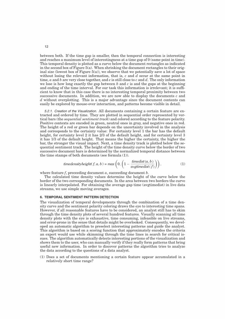
intervals get much more space than they would with linear time scaling and can easily be analyzed in detail without any overlap. For each feature one individual time den­sity plot is created. The threshold that determines when detailed temporal relations are displayed depends on the average frequency of the respective feature. Thus, data streams and features of very different temporal resolutions and granularities (as they appear in our data) can be readily handled in the same manner. This novel approach can be generalized for application scenarios, where such temporal accumulations of comments are the main interest. Our basic visualization consists of two parts that require the same space each, a sequential sentiment track on top and a time density track below; see Figure 5(b) for an example. The sequential sentiment track contains all documents mentioning a feature of interest in sequential order as they occur along the time dimension. The exact point in time is not relevant in this upper track, only the temporal order is maintained, so that both space-consuming gaps and overplotting are inherently avoided. Each rectangle bar encodes one document that contains the feature and indicates by its color the polarity of the feature. The height of a bar de­pends on the certainty level of the analysis, that is, the more certain the analysis, the higher the bar. The space that is needed in horizontal direction thus depends linearly on the number of documents in which the feature appears. Figure 5(a) provides details and an example on how the time density track is created. In the upper box, documents a, b, c, d, and e are plotted as rectangles on a time line. Document c and d have exactly the same time stamp and are thus plotted one on top of the other. The time distance between each pair of consecutive documents is given in the figure; for simplicity let us assume we have an overall time interval of 100 minutes. Then, a appears after 25 minutes, b after 30 minutes, and so on. As we observe 5 documents within 100 minutes we assume that if they were equally distributed over time, every 20 minutes we should be able to observe one document, as this is the average time distance between succes­sive documents. Therefore, we define that if the time gap between two documents is larger than the average (here: 20 minutes) there is no noteworthy temporal connection

12

between both. If the time gap is smaller, then the temporal connection is interestingand reaches a maximum level of interestingness at a time gap of 0 (same point in time).This temporal density is plotted as a curve below the document rectangles as indicatedin the second box of Figure 5(a). When shrinking the document rectangles to their orig-inal size (lowest box of Figure 5(a)), we observe that we potentially save a lot of spacewithout losing the relevant information, that is, c and d occur at the same point intime, a and b are very close together, and e is still close to c and d. The only informationwe lose is how long exactly the gap between b and c is and the gaps at the beginningand ending of the time interval. For our task this information is irrelevant; it is suffi-cient to know that in this case there is no interesting temporal proximity between twosuccessive documents. In addition, we are now able to display the documents c andd without overplotting. This is a major advantage since the document contents caneasily be explored by mouse-over interaction, and patterns become visible in detail.

5.2.1. Creation of the Visualization. All documents containing a certain feature are ex-tracted and ordered by time. They are plotted in sequential order represented by ver-tical bars (the sequential sentiment track) and colored according to the feature polarity.Positive contexts are encoded in green, neutral ones in gray, and negative ones in red.The height of a red or green bar depends on the uncertainty involved in the analysisand corresponds to the certainty value: For certainty level 1 the bar has the defaultheight, for certainty level 2 it has 2/3 of the default height, and for certainty level 3it has 1/3 of the default height. That means the higher the certainty, the higher thebar, the stronger the visual impact. Next, a time density track is plotted below the se-quential sentiment track. The height of the time density curve below the border of twosuccessive document bars is determined by the normalized temporal distance betweenthe time stamps of both documents (see formula (1)).

timedensityheight( f, a, b ) = max

(

0,

(

1 −timedist (a, b )

avgtimedist ( f )

))

, (1)

where feature f, preceeding document a, succeeding document b.The calculated time density values determine the height of the curve below the

border of the two corresponding documents. In the area between two borders the curveis linearly interpolated. For obtaining the average gap time (avgtimedist) in live datastreams, we use simple moving averages.

6. TEMPORAL SENTIMENT PATTERN DETECTION

The visualization of temporal developments through the combination of a time den-sity curve and the sentiment polarity coloring draws the eye to interesting time spans.However, if all reasonable features have to be considered, an analyst still has to skimthrough the time density plots of several hundred features. Visually scanning all timedensity plots with the eye is exhaustive, time consuming, infeasible on live streams,and error-prone in the sense that details might be overlooked. Consequently, we devel-oped an automatic algorithm to preselect interesting patterns and guide the analyst.This algorithm is based on a scoring function that approximately encodes the criteriaan expert would use while skimming through the time lines in search for critical is-sues. The algorithm automatically detects interesting portions of the visualization andshows them to the user, who can manually verify if they really form patterns that bringuseful new information. In order to discover patterns the algorithm tries to analyzethe data according to the questions of a data analyst.

(1) Does a set of documents mentioning a certain feature appear accumulated in arelatively short time range?

13

(2) Is this subset dominated by negative sentiments about the feature?(3) Is the feature mentioned in similar contexts, that is, do people report about the

same issue or about different ones?

The first question can be answered separating documents according to the occur-rence of features and investigating their temporal distribution. In order to detectinteresting time patterns within the documents mentioning a specific feature, firstcandidate time pattern intervals have to be identified. A candidate pattern is anypattern that corresponds to a relatively large interval of documents with high timedensity. Time-dense means that all time distances between consecutive documents inthis interval are smaller than the average (for the current feature). Visually this cor-responds to a portion of the time density curve that is constantly above zero, withoutinterruption. An interval is considered to be large if it is at least twice as long asthe average time-dense interval for the same feature. In addition, as the main goalis to detect problems, intervals that are dominated by negative feedback are of priorinterest. Thus, if an interval according to our criteria is both time-dense and large,and if it contains more negative than positive comments, it is inserted into the can-didate pattern list and regarded for further analysis. The following algorithm detailsthe detection of such candidate intervals.

Algorithm to extract candidate patterns for individual features:Definition

pattern = list of tuples (time distance, sentiment value);Input

L_t := List of ordered time stamps (for one feature)L_s := Corresponding list of sentiment values

multiplied with certainty valuesDerived

L_d := List of pairwise time distances of succeedingtime stamps (calculated from L_t);

d_avg := Average pairwise time distance of succeedingtime stamps (calculated from L_d);

L_p := new empty list of patterns;p_tmp := pattern, initialized with null;

for d at k in L_dif d < d_avg

if p_tmp is nullp_tmp := new empty pattern;

endifadd (d, L_s[k]) to p_tmp;

endifelse

if p_tmp is not nullif isNegative(p_tmp)

add p_tmp to L_p;endifp_tmp:= null;

endifendelse

endfordeleteShortPatterns(L_p)

14

OutputL_p

where- isNegative(pattern p) returns true if the sum of all sentimentvalues in pattern is negative- deleteShortPatterns(List of patterns L_p) deletes patterns that haveless than 2 times the average pattern length for the same feature.

Next, all candidate interval patterns for a feature F are scored and ranked with respectto their importance for analysts. The score was empirically designed and consists offour factors.

(1) DENSITY: The average height of the time density curve for a candidate pattern.The higher the curve is on average, the more densely the documents appear intime. In order to account for the undesired influence of uninteresting events on thetime density, the fraction of uninteresting events is incorporated as a compensatingweight. In the detection of negative sentiment patterns, for example, uninterestingevents correspond to documents mentioning a feature F with positive sentiment S.In general, the smaller the relative time distance D(x) of a document x to the nextdocument within the pattern P, the higher the density value of P. The time dis-tance is normalized with the average time distance avg(D(F)) among consecutivedocuments mentioning feature F.

density(P) =1

|{x ∈ P}|

∑

x∈P

(

1 −D(x)

avg(D(F))

)

·

(

1 −|{S(x) : S(x) > 0}|

|{S(x)}|

)

(2) SMOOTHNESS: The time density curves of many interesting patterns have ashape that clearly shows an increase, a plateau, and a subsequent decrease. Onthe other hand there are larger patterns of events that are rather loosely con-nected in time, showing a zigzag pattern. The latter ones are usually less interest-ing, and this is why we give a higher score to patterns with smoother time densitycurves. The smaller the average normalized difference of succeeding time distancesD among the documents x within the pattern P, the higher is the smoothness valueof pattern P. Note that all time distances D necessarily are smaller than the aver-age time distance for the same feature F as this is a criterion for being a candidatepattern.

smoothness(P) = 1 −1

(|x ∈ P| − 1)

i<(|x∈P|−1)∑

i=0

∣

∣

∣

∣

D(xi)

avg(D(F))−

D(xi+1)

avg(D(F))

∣

∣

∣

∣

(3) SENTIMENT-NEGATIVITY. The more negative the documents in a candidate pat-tern are, the more it might point to critical issues. The higher the certainty of thesentiments, the more interesting. Therefore, the sentiments S on the feature in in-dividual documents x are summed up. To get a positive score when having mostlynegative sentiments, values are multiplied with -1.

sentiment-negativity(P) =∑

x∈P

−S(x)

(4) CONTEXT-COHERENCE. There may be accumulations of negative comments ona feature that do not necessarily refer to the same issue. On the other hand, thosecandidate patterns are of most interest for which all documents apparently re-port about the same issue, that is, they mention the feature in similar contexts.

15

Table I. Contingency Table Showing theNumber of Documents DOC Depending

on a Certain Term T and a CertainPattern P

DOC ∈ P DOC /∈ P

T ∈ DOC A B

T /∈ DOC C D

A simple but effective heuristic was designed to take this context coherence intoaccount. For every potentially content-bearing term (adjectives, nouns, verbs) inan candidate pattern it was evaluated how strongly this term T is associated withthe documents DOCS of a pattern P. To measure the significance of an associationthe log-likelihood ratio test was used, which operates on a contingency table (seeTable I) and has been used before to measure the strength of word collocations[Manning and Schuetze 1999].

The document counts were used to calculate the log-likelihood ratio (see Eq. (2)),where A , B, C, and D correspond to the four cells in Table I.

log-likelihood ratio = A log

(

A/(A + B)

(A + C)/(N)

)

+ B log

(

B/(A + B)

(B + D)/N

)

+C log

(

C/(C + D)

(A + C)/N

)

+ D log

(

D/(C + D)

(B + D)/N

)

with N = A + B + C + D

(2)

Next, the top 10 associated terms for a pattern are determined and their log-likelihoodratios are summed up. This sum will be higher for patterns that have a number ofterms occurring significantly more likely within the documents of the pattern thanwithin the other documents. This is the case for patterns with a coherent context for afeature.

context-coherence(P) =

10∑

i=1

log-likelihood ratio(Ti, P)

where log-likelihood ratio(Ti, P) ≥ log-likelihood ratio(Ti+1, P)

OVERALL SCORE. All four outlined factors get equal influence in the score of a pat-tern P, as shown in the formula that follows.

score(P) = density(P) · smoothness(P) · sentiment-neg.(P) · context-coh.(P)

In a series of experiments on different test datasets (customer Web surveys, RSS news,and Twitter data) this score function yielded a very satisfying performance. However,it is possible for the analyst to adapt the weighting among the factors according to thecurrent focus of search. The default score makes it possible to find interesting patternsquickly without requiring any preknowledge about the data or deeper insight into thealgorithm. The effectiveness of the scoring function is described in Section 8 (evalu-ation), where also the influences of the individual factors on the overall performanceare shown.

6.1. Possibilities for Live Alerting

The whole pipeline of suggested methods (see Figure 2) is able to work on live datasetswith continuous updates. The only prerequisite is to have a limited amount of past

16

data in order to determine the moving average time density values for the differentfeatures. Then, each new customer feedback comment can be aggregated to the corre-sponding feature time lines as soon as it comes in. Alerts can be sent out right away ifa feature reaches considerably high scores. This automatic tracking of large numbersof different features puts analysts into the position of being able to instantly detectemerging trends and problems. The analyst is then able to react immediately on is-sues that otherwise might not have been discovered until the comments had a negativeimpact.

7. APPLICATION CASE STUDIES

One difficulty in the evaluation of an approach that helps to visually detect interestingtemporal sentiment patterns in large documents streams is the lack of appropriateground truths. For two datasets, however, we were able to get at least some basicground truth. In the following application case study we provide empirical evidenceand examples for the good performance of our method, by comparing its results withthese basic ground truths.

7.1. Customer Web Surveys

With the help of the data manager, who had provided the customer Web surveys, wewere able to construct a ground truth of known issues that had occurred in the timespan of the dataset (about 2 years); see Section 8.1 for details. We ran our automaticpattern detection algorithm and extracted the top 10 patterns; see Table II. One ofthose patterns was a false positive (issue 6) and two further patterns relate to knowngeneral problems that could not in particular be related to the determined time span(issue 4 and 8). The remaining issues had all been contained in the ground truth. Itcan be seen that patterns are detected in the feature time series of both frequent fea-tures, like “phone”, overall 1650 comments, and infrequent features like “packing list”,44 comments, or “customs”, 26 comments. The two latter ones can otherwise easilyremain undiscovered because of their infrequency. Even the top issue “password”, 129comments, is relatively infrequent considering the overall amount of documents (seeFigure 4). The spike is only visible in the time density plot and coincided with a loginissue that was not immediately corrected because it was not known at the time. Fur-ther detected issues cannot be discussed in detail, because of the confidentiality of thedata. The data manager stated that he learned several interesting things about hisdata and, during the ground-truth construction, discovered issues with help of the toolthat he had not been aware of. In general, it can be observed that patterns may havevarying time spans. In this dataset the available time resolution is on day basis anddiscovered issue time spans range from single days to several weeks. In Table II it canbe seen that the wrong detection of issues 4, 6, and 8 is an artifact of having a timeresolution on day basis. All of the wrongly discovered features are comparatively fre-quent and mostly negative. One feature mention per day is enough to keep their timedensity curves above 0. Apparently, this increases the chance to produce meaninglesspatterns.

7.2. RSS News on Electoral Campaigns

RSS news feed items mentioning the presidential candidates and their parties werecollected in the three weeks before the U.S. presidential election in 2008. With theformer approach three interesting events with negative sentiment connotation wereidentified in this time range (see Wanner et al. [2009]).

(1) Sarah Palin was accused of abusing her power as Alaska’s governor firing thestate’s public safety commissioner (“Troopergate”).

Table II. The Top Ten Issues Discovered by 1he Automatic Pattern Detection

·4 , Indi:a (cnattab) Tue Sep 18 ?.9Q7 -Thu Oct 04 2007

s, •oft•ai'&­MiJa Nov 26 ;;t007 ._ Sat Dec. 15 :2007

a . •nst~~h Tuc Nav .2'1 2007 ~ Tl;au t>o~ 9fi 2007

Vlsubl Patt$rn A$$oclat.e d Thrtlls

u1any, emaU a.ddrn:~, not to accept, web:dte,

uuaue:ceadul, phone, t.o t ry, to f$ il, timo

wrong, tot$.1, to 4b.ow, firs t, order confirmatJon~ nmount\ to di~n.pp<>int,

cou.fu.sion, accessory

hour, many, technical , l'll\Jl'IC:, b~t.~ic, f'i r1et , ll<'!rvice

peraon, t-o try, httrd

c~lurteO.u:t 1 lnn~riea.n, n Qt to understl.'.nd, <So meone, personnel, world, people,

folk, not good

to bold up. t..o dcl~y, paperwork, s ut"e, day,

indiAnllpoli.'l, pl:'por -work, not correct.., to hold

not same, aame, product ·~JJO<:, (abo, (;$r , promi:se.,

photos, compute.r, caU

n()t t.o r ecycle, cn-rtridc-e, not to inc lude, to recycle, new, n.ot t <) dlapose, not

to prin, , photo.sml:'rt c6380, t~cy(lle

noi to 3PC<'k. poor, too apeak, wrons, new, not .nicQ, not to u»d~rst-'nd,

hour , rep

oo , happy, old, basic, pTQKJ"arn, Qt.ber , nQt ne.w,

l\ow. not eom.pa.tiblo

£i r$l 0 wr<)n&, l\.ble, india, rep, to ta.ke, to c.-.11, few.

hour

In the left column issues contained in the ground truth are colored in red, general issues in yellow, and false positives in green. If two discovered features relate to the same issue, that is, they shared at least 50% of the documents contained in their patterns, they are regarded as one issue and only the plot of the higher-scored feature is displayed. The lower-scored features are added in parentheses.

17

18

1. Issue: "grandmother"

Man oct2D 200819:47-- Tue 0d 21 2001Z2:14 Alsoclat~m; to vbit to aei'Vt:, hawaii, ts-·ytar-old. til, wnt palm, campaicn tYent, to u nc:e:l. akk

2. Issue: "supremacist"

Associations: white, supremacist. killilncsPfee, natloNI, to p1ot, to 10, to disrupt. fed, s.klnhe•d plot. nnat

No big topic: "health insurance"

Many Amttklns do not have • health insunM'Ioe..

Fig. 6. Time density plots of the two top issue features and of a further feature "health insurance" that apparently did not play a big role in news about the electoral campaign.

(2) A plot of white supremacists to assassinate Barack Obama was uncovered. (3) Obama and McCain attacked each other and battled fiercely in a TV debate.

Surprisingly, the top pattern detected by our algorithm (feature "grandmother") cor­responds to a negative event (see Figure 6), that had not shown up in the previous analysis: Barack Obama interrupted his campaign to visit his gravely ill grandmother. Further patterns among the top 10 dealt with the known assassination plot and the Troopergate scandal. Another new issue was discovered at rank 10: Barack Obama's aunt was living illegally in the US. In the top 20 patterns further previously undis­covered issues were detected: Palin and McCain accused Obama of not being honest about his association with a former war protester. In a further issue they accused the Los Angeles Times of withholding a videotape showing Obama attending a party for a Palestinian-American professor and critic of Israel. Furthermore, one issue reveals that Palin took a prank call from a Canadian comedian posing as French President. Also, a voter registration fraud is reported.

However, the tv debate issue did not make it among the top patterns because it was not very negative. In general it could be observed that many different sources post very similar news within short time spans that are only slight variations of news agency messages. This facilitates the discovery of patterns.

It is also possible to track any topic of interest and try to visually detect patterns. Figure 6 shows the example of the feature "health insurance": It can be seen that it was not a big topic and did not mainly have negative connotations.

8. EVALUATION AND DISCUSSION

In addition to the application case study, further parts of our approach are evaluated individually: the automatic pattern detection (Section 8.1) and the modeling of uncer­tainty (Section 8.2). In Section 8.3 an expert user study is provided to give further insight into the r eal-world applicability and usability of the system. Along the evalua­tion different features and limitations of our approach are discussed.

8.1. Automatic Pattern Detection

For the customer Web survey dataset a ground truth of important issues was con­structed. The data analyst who provided the dataset and had been working with it during data collection was able to name 9 important issues that he was aware of. In addition, among the automatically extracted issues, he was able to identify 8 further issues interesting to him. With this ground truth of 17 time-related issues to be found we evaluated the precision and recall of the automatic pattern detection algorithm. To

19

All factors Without eontext-c:otterenoe Wlthovl smoothness

!3

~ !3

~ ~

~ ~ - :; d s d & d .~ d

l ..

l ~ 1 "' ~ 0

:;; :;; ~

:l :l ~ o.o 0.2 o.• 0.6 0.8 1.0 0.0 0.2 0.4 0.6 o.a 1.0 o.o 0.2 0.4 0.6 o.a 1.0

recall ...... - JJ

Wllhout density Wllhout unc0f1ainty Without sentiment-negativity

!3

k ~

~ !3

~ a a :; -

i ..

t ~ i d 0

.. ~ ~ a ~

:;; "! 0 ~·-

0 :l :l 0

0.0 0.2 0.4 0.6 o.a 1.0 0.0 0.2 0.4 0.6 0.8 1.0 o.o 0,2 OA 0.6 0.8 1.0

fetolli - -Fig. 7. Recall-precision diagrams for the score containing all factors (upper left) and modified scores where one factor is excluded. In these diagrams the recall-precision curve for the score with all factors is addition­ally displayed in black to enable comparison.

Table Ill. Precision and Recall Values when Extracting the Top 20 Patterns

Method Precision Recall Original Score 60.00% 70.59%

Without Sentiment-Negativity 55.00% 64.71%

Without Density 50.00% 58.82%

Without Smoothness 50.00% 58.82%

Without Uncertainty 45.00% 52.94%

Without Context-Coherence 40.00% 47.06%

this goal, the top 20 patterns according to the overall score were extracted and it was verified whether these patterns actually pointed to one of the 17 known issues. The recall-precision diagram for the overall score is displayed in the upper left of Figure 7. Taking all 20 results, the precision is 60.00% and the recall 70.59%. In addition, the results for modified scores are provided, performing a sensitivity analysis. For each of the other scores one factor of the overall score was left out and again a recall-precision diagram was created (Figure 7). The purpose of this sensitivity analysis was to validate that each factor in the score is actually beneficial, which is true if all top 20 results are considered; see Table Ill. However, the version that does not consider the sentiment­negativity partly outperforms the overall score when returning less than 20 results, as can be seen in Figure 7. Apparently, the exact negativity of a pattern is not that important as long as it is assured that the negative comments dominate. Even more astonishing is that the uncertainty has a beneficial influence on the overall score, al­though it just modifies the sentiment-negativity. We could observe that the uncertainty was preventing features that at the same time were sentiment words (e.g., problem, waste, error) from being weighted too much. The tmcertainty modeling causes these kind of features to get certainty value 1/3 if no other sentiment words can be found in their surroundings. From Table ill and Figure 7 it can also be deduced which among

20

Table IV. Results of the Sentiment Analysis Dependent on the Certainty Level

Dataset Level 1 Level 2 Level 3 No Sentiment

Customer Feedback Accuracy 85.7% 84.8% 80.0% 19.7 %

Customer Feedback Proportions 27.9% 39.3% 2.5% 30.3%

RSS Feeds Accuracy 80.0% 52.9% 62.5% 74.6%

RSS Feeds Proportions 14.9% 51.7% 4.0% 29.4%

All values are rounded to one decimal. The proportions show the fraction of all featurementions the algorithm assigned with the corresponding certainty level. The accuracyshows which fraction of the feature mentions of one certainty level have been assignedto the correct sentiment category (positive, negative, neutral).

the factors are most valuable when trying to detect interesting patterns. Surprisingly,the context coherence has the strongest positive effect on the score, which becomes evi-dent by the much worse performance when leaving it out. Next, the uncertainty has thesecond best influence, although it is not a real factor in the formula, but just a modify-ing element of the sentiment-negativity. Density and smootheness both cause the sameimprovement which still is a considerable contribution. Only the sentiment-negativitycannot unambiguously be classified as being beneficial. Interestingly, the good per-formance without this factor is due to the fact that some issues have been identifiedthat had not been detected in any of the other settings. This was the case when theautomatic sentiment analysis could not detect many negative statements, but the cor-responding issue still was in the ground truth. While sentiment analysis apparentlyis rather simple for some features, other features contain many implicit sentimentsand get higher scores when the sentiment-negativity is not even considered. It can beconcluded that whenever the sentiment analysis is accurate it is beneficial to includesentiment-negativity.

8.2. Uncertainty Assessment

It is well-known that automatic sentiment analyses cannot be 100% accurate, dueto different reasons (ambiguity, implicitness, etc.). To enable analysts to judge howconfident analysis results are, in our approach the uncertainty involved in the analysisis assessed and visually conveyed. To evaluate the uncertainty modeling, for both thecustomer Web surveys and the RSS news feeds, 201 feature mentions were annotatedmanually. For each dataset the first 3 mentions of the 67 most frequent features wereconsidered. This was done in order not to bias the results, because sentiments appearto be easier to detect for some features than for others. The resulting values areprovided in Table IV. The numbers are quite different for both datasets and in generalbetter for the customer Web surveys, for which the analysis had been designed firstof all. For these surveys there are no considerable differences in accuracy among thethree levels, which would be a good argument to omit them. However, as shown inthe evaluation of the pattern detection (Section 8.1), it is still beneficial to considerthe uncertainty, because it works better for the special case where words are featuresand sentiments at the same time. The value in the category “No Sentiment” showshow many of the feature mentions, for which no sentiment could be identified,actually did not have any sentiment. In other words a low accuracy here indicatesthat quite a number of sentiments have not been detected, which is the case for thecustomer Web surveys. This is quite different for the RSS feeds dataset. Apparently,this contains many more nouns not mentioned in relation with a sentiment thanthe customer surveys. In addition, a clear difference between level 1 and the twoother levels is visible. Considering the fact that the algorithm has three options forsentiment labels (positive, negative, neutral), the 52.9% accuracy for level 2 is still

21

0 _;_

(b) (c) (d)

Fig. 8. Numerical results of the study: (a) time-related issues detected correctly within 20 minutes (average per person), (b) confidence in discovering time-related issues (per issue) on a scale ranging from 1 (not very confident) to 5 (absolutely confident), (c) estimated amount of comments read (per discovered time-related issue), (d) overall amount of comments read by each participant including comments that did not lead to the discovery of time-related issues.

much better than chance but at the same time not quite satisfying. One reason is that in news about electoral campaigns the different political camps are often named in the same sentence, either comparing them or citing representatives of one camp talking about the opponents. In these cases our automatic sentiment analysis has problems attributing sentiments to the correct entity. For the automatic pattern detection, however, this flaw typically is not a big problem as sentiment-negativity was shown to be less influential than the other parameters.

8.3. Expert User Study

In order to gain a better understanding of the usefulness and usability of the system for target users an expert user study was conducted. We were able to get hold of 7 ex­perts willing to participate. The participants were asked to use the system to identify important time-related issues contained in the Web survey dataset. To this end, they were first given explanations about the underlying concepts of the visualizations con­tained in the tool and were given the chance to become familiar with the possibilities for interaction. This introductory phase took about 5 to 10 minutes depending on the questions a participant had about the techniques and the tool. Then, the participants were given 20 minutes to find as many time-related issues as possible. Moreover, they were asked to speak their thoughts aloud during the whole study, so it would be easier for the observing person to learn more about their strategies, assumptions, and prob­lems when using the tool. For each time-related issue a participant believed to have found she/he should provide further information: the feature that had helped to dis­cover the issue, a short description of the issue, the start and end time, the estimated number of comments read to identify and understand the issue, and finally the con­fidence in this analysis. The purpose of asking for a description of the issue as well as the start and end was to assure that the participant actually had gained an under­standing of the issues he or she discovered and was able to identify time ranges. The further information was collected to evaluate the reading efforts required and the con­fidence participants had gained in their analysis. As well, participants were given the option to state that they had discovered an issue that did not appear to be time-related but rather general. Finally, the participants were asked whether they considered the tool as being useful and if so what they liked the most. Further questions were what they disliked about it and what suggestions for improvement they had. Also, they were asked whether they ran out of time and thought they could have discovered more is­sues easily or if already within the given time they had problems discovering further issues.

22

Table V. The Aggregated Results for All Participants

Truly time-related Truly general Truly nothing

Time-related (participant) 35 0 3

General (participant) 2 10 0

Nothing (participant) 1 1 7

The choices of the participants (rows) in comparison with the ground truth (columns),only for those features participants actually had a chance to look at before running outof time.

Results and Discussion. First, we want to look at the quantitative performance shownin Figure 8. In average participants were able to discover 5 time-related issues within20 minutes and had to read 9.84 comments to verify them. They were pretty confidentin the analysis with an average of 4.45 (with 5 being the maximum and 1 the min-imum). Only 3 (7.9%) false time-related issues were identified, aggregating resultsfor all participants. The 3 false hits correspond exactly to those that were identifiedwith a confidence of 3 or lower. The overall amount of comments read (Figure 8(d))varies considerably. It could be observed that some participants read comments onlysuperficially focusing on the sentences containing the feature, while others read com-ments completely. The 74.57 comments participants read in average during the studyonly correspond to about 0.15% of the overall data (50,000 comments). Next, TableV shows the aggregated performances of all participants for all features which theymanaged to investigate within the 20 minutes. The overall precision is 88.14%, theprecision for time-related issues 92.11%. The 5 time-related issues participants wereable to detect in average correspond to a recall of 29.41%. However, the trade-offintroduced by the fixed time constraint is decisive here. All 7 participants were con-fident that they would have discovered more issues if having more time. At the sametime, one participant commented that if it was critical in a real-world analysis hewould have read every single comment of an interesting time interval pattern, whichhe did not during the study. All in all, the numerical evaluation of the performanceproved that the system is actually usable and suitable for the outlined task of identi-fying time-related issues in large sets of documents minimizing the reading efforts foranalysts.

More interesting than the numerical performance, however, were insights gainedwhen observing the experts using the tool. A basic strategy all participants sharedwas starting to have a closer look at the intervals automatically detected by the au-tomated analysis. Yet, to our surprise participants applied quite different individualstrategies to deal with these intervals. One participant first had a look at differentinteresting time density plots without exploring them in detail, in order to gain a bet-ter feeling for the visualization. In general, users got faster and more accurate thelonger they worked with the tool. When running out of time one user commented thathe probably had misinterpreted something at the beginning and had just realized thisafter researching further time density plots, which was actually true. When it came toexploring potentially interesting intervals, one user preferred reading negative com-ments with a high level of certainty while another user first read the comments at thebeginning and end of the highlighted area to see whether they were similar. Severalusers tended to ignore comments with neutral rating and rather read the other com-ments. A further user preferred to first read the associated terms of a highlighted areaand only then started reading; he was the one that read the least number of commentsto identify issues. While 4 participants focused mainly on reading comments withinhighlighted intervals the other 3 also read a considerable number of comments outsideintervals to see whether the reported issue might have persisted in time but just with

23

a lower frequency. In general it could be observed that the more homogeneous in con-tent the comments within an interval were, the quicker an issue was detected. Thiswas more often the case when dealing with generally infrequent features than withfrequent ones.

The answers to the survey questions at the end of the study revealed further details.All participants found the tool useful and when asked what they liked most made thefollowing responses (several things could be named by one participant): 6 mentionedthe automatic scoring and highlighting of interesting intervals, 3 mentioned the quickaccess to the documents via mouse-over, and 2 named the combination of sentimentand time density track. Not liked about the tool was that when zooming out too far,objects could disappear from the screen. This was mentioned by 4 participants andcould be fixed in the meantime. Another complaint was about the insufficient descrip-tion of the interface and one user would have liked an auto-size functionality to see awhole time density plot on the screen without zooming by himself. Further suggestionsfor improvement were given. One participant would have liked to be able to searchand highlight keywords, respectively highlight comments in which these keywords ap-peared. She wanted to see whether certain keywords appeared more frequently withinthe comments of an interval than outside. Another participant would have liked tobe able to combine two features to one time density plot, containing only documentswhere both selected features appeared.

As mentioned before, the target user group for our approach and also within theuser study were experts. Of course, experts in data analysis are a very experienceduser group, so the results cannot simply be generalized to common computer users.The similar level of experience of the participants may also have contributed to therelative homogeneity in performance, though their strategies were quite diverse. Inconclusion, the basic concept was well-received, participants gave a mostly positiveinformal feedback, and were able to identify time-related issues without larger readingefforts. Apart from fixing minor interaction problems further methods for filtering andselection should be integrated in future versions.

9. CONCLUSION

In this article, we address a feature-based sentiment analysis process that tightlycouples methods from automatic text processing, visual analytics, and informationvisualization. Our intelligent visual interface for several reasons is especially ben-eficial to explore sentiments over time. First, the uncertainty involved in automaticanalysis due to the complex and ambiguous nature of language requires furtherexploration: The textual content of customer comments can easily be accessed bymouse-over interaction for detailed insight and to derive meaning. Second, the factthat it is not quite clear beforehand what kind of interesting temporal patterns mightbe included in the data demands a broad feature coverage and visual exploration. Toquickly analyze vast volumes of text documents over time, we use two complementaryvisualizations: pixel map calendars for general overview and sequential time densityplots for detailed insights. Features of interest can be selected and visually exploredfor salient patterns, combining both visualizations. Furthermore, interesting intervalpatterns are automatically detected and scored. The score measures the importanceof an interval based on the height and smoothness of the time density curve, thesentiment negativity, and the context coherence. Analysts can use this score to auto-matically detect top issue patterns potentially also for early prevention in real time.Our new solutions were tailored for direct customer feedback through Web surveysand further tested on RSS news feeds. Previously unknown issues were discoveredand features of interest could be explored in detail. In an extensive evaluation wewere able to demonstrate the applicability, usability, and good performance of the

24

approach, learned about the impact of different parameters, and discussed limitations.Our future research will be in the areas of real-time visual sentiment comparison andreasoning.

ACKNOWLEDGMENTS

The authors wish to thank Meichun Hsu for her suggestions and encouragement.

REFERENCES

AIGNER, W., MIKSCH, S., MULLER, W., SCHUMANN, H., AND TOMINSKI, C. 2007. Visualizing time-orienteddata - A systematic view. Comput. Graph. 31, 3, 401–409.

ARIS, A., SHNEIDERMAN, B., PLAISANT, C., SHMUELI, G., AND JANK, W. 2005. Representing unevenly-spaced time series data for visualization and interactive exploration. In Proceedings of the INTERACTConference. 835–846.

DING, X. AND LIU, B. 2007. The utility of linguistic rules in opinion mining. In Proceedings of the 30thAnnual International ACM SIGIR Conference on Research and Development in Information Retrieval(SIGIR’07). ACM, New York, 811–812.

DING, X., LIU, B., AND YU, P. 2008. A holistic lexicon-based approach to opinion mining. In Proceedings ofthe International Conference on Web Search and Web Data Mining. 231–240.

HAO, M. C., KEIM, D. A., DAYAL, U., OELKE, D., AND TREMBLAY, C. 2008. Density displays for data streammonitoring. Comput. Graph. Forum 27, 3, 895–902.

HAVRE, S., HETZLER, E., WHITNEY, P., AND NOWELL, L. 2002. Themeriver: Visualizing thematic changesin large document collections. IEEE Trans. Vis. Comput. Graph. 8, 9–20.

KIM, S.-M. AND HOVY, E. 2004. Determining the sentiment of opinions. In Proceedings of the 20th Interna-tional Conference on Computational Linguistics (COLING’04). Association for Computational Linguis-tics, 1367–1373.

KISILEVICH, S., ROHRDANTZ, C., AND KEIM, D. A. 2010. “Beautiful picture of an ugly place”. Exploringphoto collections using opinion and sentiment analysis of user comments. In Proceedings of the Compu-tational Linguistics & Applications Conference (CLA’10). 419–428.

KRSTAJIC, M., MANSMANN, F., STOFFEL, A., ATKINSON, M., AND KEIM, D. A. 2010. Processing onlinenews streams for large-scale semantic analysis. In Proceedings of the 1st International Workshop onData Engineering Meets the Semantic Web.

LIU, B. 2010. Sentiment analysis and subjectivity. In Handbook of Natural Language Processing 2nd Ed.,N. Indurkhya and F. J. Damerau Eds., CRC Press, Boca Raton, FL.

LIU, B., HU, M., AND CHENG, J. 2005. Opinion observer: Analyzing and comparing opinions on the Web.In Proceedings of the 14th International Conference on World Wide Web (WWW’05). ACM, New York,342–351.

MANNING, C. D. AND SCHUETZE, H. 1999. Foundations of Statistical Natural Language Processing 1st Ed.The MIT Press.

MIAO, Q., LI, Q., AND DAI, R. 2009. Amazing: A sentiment mining and retrieval system. Expert Syst.Appl. 36, 3, Part 2, 7192 – 7198.

NG, V., DASGUPTA, S., AND ARIFIN, S. M. N. 2006. Examining the role of linguistic knowledge sources in theautomatic identification and classification of reviews. In Proceedings of COLING/ACL Main ConferencePoster Sessions. 611–618.

OELKE, D., HAO, M., ROHRDANTZ, C., KEIM, D. A., DAYAL, U., HAUG, L.-E., AND JANETZKO, H. 2009.Visual opinion analysis of customer feedback data. In Proceedings of the 2009 IEEE Symposium onVisual Analytics Science and Technology (VAST’09). 187–194.

PANG, B. AND LEE, L. 2008. Opinion mining and sentiment analysis. Found. Trends Inf. Retr. 2, 1–2,1–135.

POPESCU, A.-M. AND ETZIONI, O. 2005. Extracting product features and opinions from reviews. In Proceed-ings of the Conference on Human Language Technology and Empirical Methods in Natural LanguageProcessing (HLT’05). Association for Computational Linguistics, 339–346.

QIU, G., LIU, B., BU, J., AND CHEN, C. 2009. Expanding domain sentiment lexicon through double propa-gation. In Proceedings of the 21st International Joint Conference on Artifical Intelligence. 1199–1204.

RILOFF, E. AND WIEBE, J. 2003. Learning extraction patterns for subjective expressions. In Proceedings ofthe Conference on Empirical Methods in Natural Language Processing. Association for ComputationalLinguistics, 105–112.

25

VIEGAS, F. B., WATTENBERG, M., AND DAVE, K. 2004. Studying cooperation and conflict between authorswith history flow visualizations. In Proceedings of the SIGCHI Conference on Human Factors in Com-puting Systems (CHI’04). ACM, New York, 575–582.

WANNER, F., ROHRDANTZ, C., MANSMANN, F., OELKE, D., AND KEIM, D. A. 2009. Visual sentiment anal-ysis of rss news feeds featuring the us presidential election in 2008. In (IUI’09) Workshop on VisualInterfaces to the Social and the Semantic Web (VISSW). Online Proceedings.http://ceur-ws.org/Vol-443/paper7.pdf.

WU, Y., WEI, F., LIU, S., AU, N., CUI, W., ZHOU, H., AND QU, H. 2010. OpinionSeer: Interactive visualiza-tion of hotel customer feedback. IEEE Trans. Vis. Comput. Graph. 16, 6, 1109–1118.