Feasibility Study on SAR Systems on Small Satellites - UPCommons
84
Feasibility Study on SAR Systems on Small Satellites by Albert García Mondéjar Paco López Dekker, Project Advisor Barcelona, January 2009
Transcript of Feasibility Study on SAR Systems on Small Satellites - UPCommons
Feasibility Study on
SAR Systems on
Small Satellites by
Albert García Mondéjar
Paco López Dekker, Project Advisor
Barcelona, January 2009


ACKNOWLEDGEMENTS
This project would not have been possible without the academic and moral support of a
large number of people.
My first debt of gratitude is to Paco, my tutor and also a very good friend. I would like
to thank the teachers from TSC for having taught me all these interesting courses in
which I have taken part.
A special thank to my family and friends for his enormous support during these years of
degree. I would like to emphasize people from A.C Telecogresca for letting me be part
of this big family.
I do not want to finish without mentioning my girlfriend Senda. She has been the most
important person in the last year and she always tries to help me. Thanks a lot for these
beautiful moments.

Contents Feasibility Study on SAR Systems on Small Satellites
CONTENTS
1 I�TRODUCTIO� ....................................................................................................... 7
1.1 GLOBAL CONTEXT OF SAR REMOTE SENSING ....................................................... 7
1.1.1 History of SAR space missions ..................................................................................... 8
1.1.2 ICC, PCOT and SARMISP ......................................................................................... 18
1.2 PURPOSE AND LIMITATIONS OF THE PROJECT ........................................................ 19
1.3 DOCUMENT CONTENT .......................................................................................... 19
2 SAR SYSTEM CO�SIDERATIO�S ...................................................................... 20
2.1 ORBITAL SAR GEOMETRY .................................................................................... 20
2.1.1 Altitude (h) .................................................................................................................. 20
2.1.2 Incidence angle (η) ..................................................................................................... 21
2.2 SENSITIVITY: RADAR RANGE EQUATION .............................................................. 22
2.3 RESOLUTION CONSIDERATIONS. ........................................................................... 23
2.3.1 Range Resolution ........................................................................................................ 23
2.3.2 Azimuth Resolution ..................................................................................................... 24
2.4 THE ANTENNA ...................................................................................................... 24
2.4.1 Minimum antenna area (zero order ambiguity analysis) ........................................... 25
2.5 AMBIGUITY ANALYSIS ......................................................................................... 26
2.5.1 Azimuth ambiguity ...................................................................................................... 28
2.5.2 Range Ambiguity ........................................................................................................ 28
2.6 PRF SELECTION. ................................................................................................... 30
2.7 SIGNAL PARAMETERS (F0, τ0, POLARIZATION) ...................................................... 32
2.7.1 Frequency Band.......................................................................................................... 32
2.7.2 Bandwidth and pulse duration. ................................................................................... 32
2.7.3 Polarization. ............................................................................................................... 33
3 SAR SYSTEM TRADE-OFFS A�D DESIG� FLOW .......................................... 34
3.1 IDEAL CASE .......................................................................................................... 34
3.2 CONSTRAINT CASE ................................................................................................ 35
3.3 DESIGN FLOW VALIDATION: TERRASAR-X “REVISITED” .................................... 36
4 S3D BETA VERSIO� (SOFTWARE FOR SAR SE�SOR DESIG�) ................. 39
4.1 IDL INTRODUCTION.............................................................................................. 39
4.2 S3D BACK-END DESCRIPTION ............................................................................... 39
4.3 S3D FRONT-END DESCRIPTION ............................................................................. 40
5 COMPACT MISSIO� DESIG� PROPOSAL ....................................................... 43
5.1 APPLICATIONS OF INTEREST ................................................................................. 43
5.1.1 Agriculture .................................................................................................................. 43
5.1.2 Forestry ...................................................................................................................... 43
5.1.3 Urban Monitoring ...................................................................................................... 44
5.1.4 Coastal and Marine Applications ............................................................................... 45
5.1.5 The Hydrologic Cycle ................................................................................................. 46
5.1.6 Cartography ............................................................................................................... 47
5.2 ORBITAL DETERMINATION. ................................................................................... 47
5.3 SMALL SAR SENSOR PROPOSAL AT L, C AND X BAND .......................................... 49
5.4 DATA STORAGE AND DOWN LINK. ......................................................................... 54

Contents Feasibility Study on SAR Systems on Small Satellites
6 SUMMARY, CO�CLUSIO�S A�D FUTURE LI�ES ........................................ 57
6.1 SUMMARY ............................................................................................................ 57
6.2 CONCLUSIONS ...................................................................................................... 57
6.3 FUTURE LINES ....................................................................................................... 58
REFERE�CES .................................................................................................................. 60
APPE�DIX A. IDL ROUTI�ES ...................................................................................... 64

Chapter 1 Feasibility Study on SAR Systems on Small Satellites
7
1 I�TRODUCTIO�
1.1 Global Context of SAR Remote Sensing
Remote sensing is the group of techniques that allow us to acquire information of objects
or phenomenon’s, without the necessity of being in contact with the object (such as by way
of aircraft, spacecraft, satellite, or ship). Remote sensing is the collection through the use
of a variety of remote devices of information on an interesting object or area. Nowadays,
when we talk about remote sensing, it generally means the use of imaging sensor
technologies including the use of aircraft and spacecraft boarded instruments, and it is
distinct from other imaging-related fields such as medical imaging.
There are two classes of remote sensing systems. Passive sensors detect natural radiation
that is emitted or reflected by the object or the area being observed. Reflected sunlight is
the most common source of radiation measured by passive sensors. Examples of passive
remote sensors include film photography, infra-red, charge-coupled devices, and
radiometers.
On the other hand, active sensors emit energy with the intention to scan objects and areas.
Imaging radar (RAdio Detection And Ranging) is an example of active remote sensing and
has become an alternative technique for observing the Earth from space.
Radar provides its own energy source and, therefore, can operate either day or night and
through cloud cover. This means that Radar technology can provide day-and-night imagery
of the Earth independently of weather conditions
A radar system has three primary functions:
• It transmits a microwave signal (from a frequency of 0.3 GHz to 300 GHz) towards
a scene.
• It receives the portion of the transmitted energy backscattered from the scene.
• It observes the strength (detection) and the time delay (ranging) of the returned
signals
A SAR, Synthetic Aperture Radar, is a coherent radar system that can generate high-
resolution images. Signal processing uses magnitude and phase of the received signals over
successive pulses to create the image.
A synthetic aperture is produced by signal processing. The aperture has the effect of
lengthening the antenna, as the line of sight direction changes along the radar platform
trajectory.
The achievable azimuth resolution of a SAR is approximately equal to one-half the antenna
length and does not depend on platform altitude. High range resolution is achieved through
pulse compression techniques. With the aim of mapping the ground surface the radar beam

Chapter 1 Feasibility Study on SAR Systems on Small Satellites
8
is directed to the side of the platform trajectory; with a antenna beam wide enough in the
along-track direction, an identical target or area may be illuminated a number of times
without a change in the antenna look angle.
Remote sensing sensors can be carried on a variety of platforms to view and image targets.
Satellites provide a large fraction of the remote sensing imagery. They have several unique
characteristics which make them very useful for observing the Earth's surface. Remote
sensing satellites are designed to follow an orbit which, in conjunction with the Earth's
rotation, allows them to cover most of the Earth's surface over a certain period of time. The
area imaged on the surface, is referred to as the swath. Imaging swaths for space-borne
sensors generally vary between tens and hundreds of kilometers wide.
Sensors on satellites generally can "see" a much larger area of the Earth's surface than
would be possible from a sensor onboard an aircraft. Also, because they are continually
orbiting the Earth, it is relatively easy to collect imagery on a systematic and repetitive
basis in order to monitor changes over time.
The geometry of orbiting satellites can be calculated accurately and facilitates correction of
remote sensing images to their correct geographic orientation and position. However,
aircraft sensors can collect data at any time and over any portion of the Earth's surface
while satellite sensors are restricted to collecting data over only those areas and during
specific times dictated by their particular orbits.
Satellite orbits are matched to the capability and objective of the sensor(s) they carry. Orbit
selection can vary in terms of altitude (their height above the Earth's surface) and their
orientation and rotation relative to the Earth.
1.1.1 History of SAR space missions
Since the first launch of a SAR satellite many other missions have been planned. In the
last five years many research centers have been planning the development of small
platforms that were able to carry SAR systems. The reduction in the orbit altitude helps to
reduce costs and the delivery time of new data information.
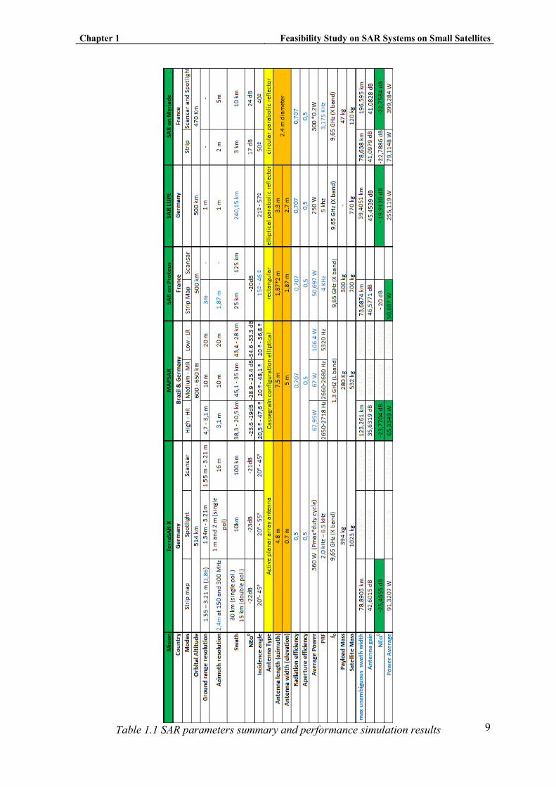
Table 1.1 summarizes the most important parameters of the recent space-borne SAR
missions. Values in blue were not available and have been simulated, calculated or
assumed.
1.1.1.1 SEASAT, 1978
SEASAT was the first Earth satellite designed for remote sensing of the Earth's oceans and
had onboard the first space-borne SAR. [1]
Chapter 1 Feasibility Study on SAR Systems on Small Satellites
9
Table 1.1 SAR parameters summary and performance simulation results
Chapter 1 Feasibility Study on SAR Systems on Small Satellites
10
The mission was designed to demonstrate the feasibility of global satellite monitoring of
oceanographic phenomena and to help determine the requirements for an operational ocean
remote sensing satellite system.
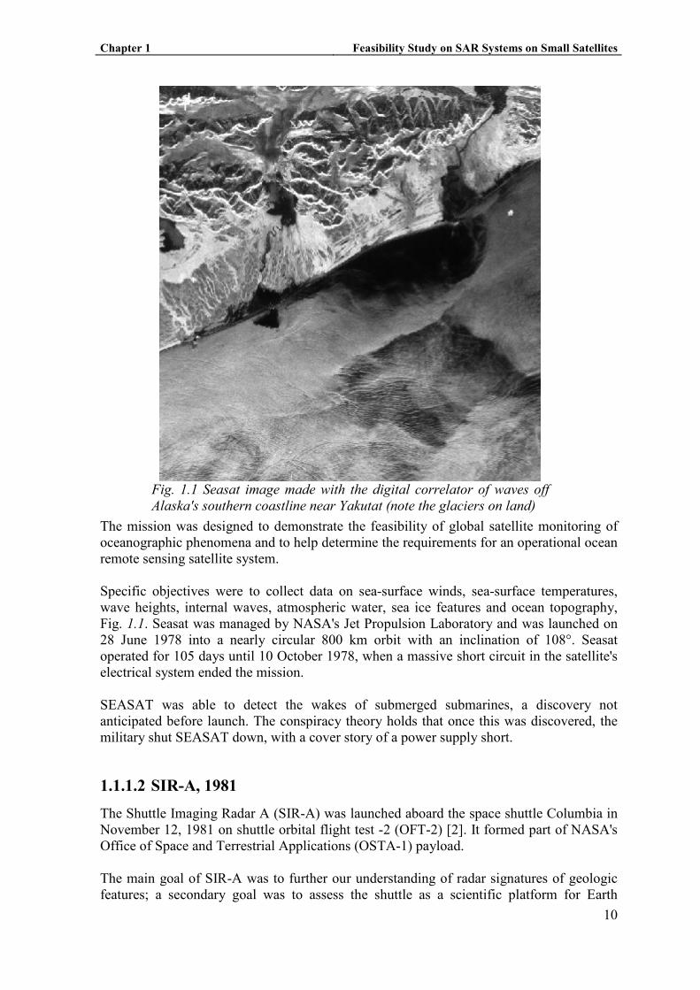
Specific objectives were to collect data on sea-surface winds, sea-surface temperatures,
wave heights, internal waves, atmospheric water, sea ice features and ocean topography,
Fig. 1.1. Seasat was managed by NASA's Jet Propulsion Laboratory and was launched on
28 June 1978 into a nearly circular 800 km orbit with an inclination of 108°. Seasat
operated for 105 days until 10 October 1978, when a massive short circuit in the satellite's
electrical system ended the mission.
SEASAT was able to detect the wakes of submerged submarines, a discovery not
anticipated before launch. The conspiracy theory holds that once this was discovered, the
military shut SEASAT down, with a cover story of a power supply short.
1.1.1.2 SIR-A, 1981
The Shuttle Imaging Radar A (SIR-A) was launched aboard the space shuttle Columbia in
November 12, 1981 on shuttle orbital flight test -2 (OFT-2) [2]. It formed part of NASA's
Office of Space and Terrestrial Applications (OSTA-1) payload.
The main goal of SIR-A was to further our understanding of radar signatures of geologic
features; a secondary goal was to assess the shuttle as a scientific platform for Earth
Fig. 1.1 Seasat image made with the digital correlator of waves off
Alaska's southern coastline near Yakutat (note the glaciers on land)

Chapter 1 Feasibility Study on SAR Systems on Small Satellites
11
observations. The satellite altitude was 265 km and operates in L-Band (frequency of 1.275
GHz).
1.1.1.3 SIR-B, 1982
Shuttle Imaging Radar B (SIR-B) was the second major step in the evolutionary NASA
radar remote sensing research program. [3]
The radar imagery collected at the fixed look angle SEASAT and SIR-A experiments
demonstrated the relationship between image intensity and the incidence angle of the radar
at the surface. This led to the design of SIR-B, the first space-borne SAR with a
mechanically tiltable antenna. This allowed the acquisition of multi-incidence angle
imagery.
SIR-B was launched on October 5, 1984 aboard the Space Shuttle Challenger on flight 41-
G into a nominally circular orbit. The average altitude for the first 20 orbits was 360 km;
for the next 29 orbits was 257 km; and for the duration of the mission 224 km. At the 224
km altitude, the orbit was allowed to drift slightly westward with an approximate 1- day
repeat cycle. This enabled SIR-B to image a given site at several different incidence angles
on subsequent days over the course of the mission.
1.1.1.4 Magellan, 1989
The Magellan spacecraft, named after the sixteenth-century Portuguese explorer whose
expedition first circumnavigated the Earth, was launched May 4, 1989, and arrived at
Venus on August 10, 1990. [4]
Magellan's solid rocket motor placed it into a near-polar elliptical orbit around the planet.
During the first 8-month mapping cycle around Venus, Magellan collected radar images of
84 percent of the planet's surface, with resolution 10 times better than that of the earlier
Soviet Venera 15 and 16 missions. Altimetry and radiometry data also measured the
surface topography and electrical characteristics.
1.1.1.5 ERS-1, 1991
European Remote Sensing satellite (ERS-1) was the first European Space Agency's Earth-
observing satellite. It was launched on July 17, 1991 into a Sun synchronous polar orbit at
a height of 782–785 km.[5]
It carried a comprehensive payload including an imaging SAR (operating in C band), a
radar altimeter and other powerful instruments to measure ocean surface temperature and
winds at sea.[6]
1.1.1.6 J-ERS-1, 1992
JERS-1, launched in Feb 1992 and finalized in Oct 1998, was a joint Japanese radar/optical
mission with NASDA/JAXA lead. [7]
Chapter 1 Feasibility Study on SAR Systems on Small Satellites
12
The overall objectives were the generation of global data sets with SAR and OPS sensors
aimed at surveying resources, establishing an integrated Earth observation system,
verifying instrument/system performances. The mission applications focused on survey of
geological phenomena, land usage, observation of coastal regions, geologic maps,
environment and disaster monitoring and demonstration of two-pass SAR interferometry
for change detection.
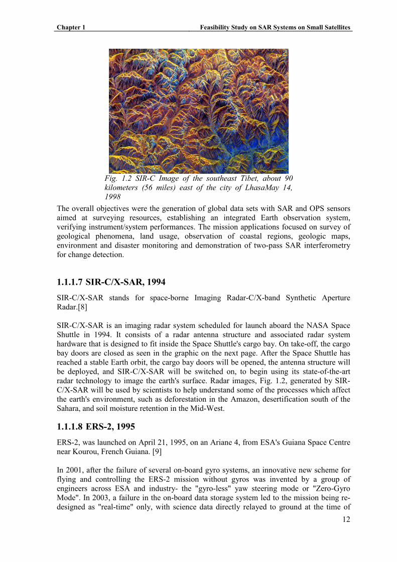
1.1.1.7 SIR-C/X-SAR, 1994
SIR-C/X-SAR stands for space-borne Imaging Radar-C/X-band Synthetic Aperture
Radar.[8]
SIR-C/X-SAR is an imaging radar system scheduled for launch aboard the NASA Space
Shuttle in 1994. It consists of a radar antenna structure and associated radar system
hardware that is designed to fit inside the Space Shuttle's cargo bay. On take-off, the cargo
bay doors are closed as seen in the graphic on the next page. After the Space Shuttle has
reached a stable Earth orbit, the cargo bay doors will be opened, the antenna structure will
be deployed, and SIR-C/X-SAR will be switched on, to begin using its state-of-the-art
radar technology to image the earth's surface. Radar images, Fig. 1.2, generated by SIR-
C/X-SAR will be used by scientists to help understand some of the processes which affect
the earth's environment, such as deforestation in the Amazon, desertification south of the
Sahara, and soil moisture retention in the Mid-West.
1.1.1.8 ERS-2, 1995
ERS-2, was launched on April 21, 1995, on an Ariane 4, from ESA's Guiana Space Centre
near Kourou, French Guiana. [9]
In 2001, after the failure of several on-board gyro systems, an innovative new scheme for
flying and controlling the ERS-2 mission without gyros was invented by a group of
engineers across ESA and industry- the "gyro-less" yaw steering mode or "Zero-Gyro
Mode". In 2003, a failure in the on-board data storage system led to the mission being re-
designed as "real-time" only, with science data directly relayed to ground at the time of
Fig. 1.2 SIR-C Image of the southeast Tibet, about 90
kilometers (56 miles) east of the city of LhasaMay 14,
1998
Chapter 1 Feasibility Study on SAR Systems on Small Satellites
13
acquisition. These in-flight adaptations have enabled the mission to be extended well
beyond its design lifetime, and recently led ERS-2 to celebrate its 60,000th orbit.
1.1.1.9 RADARSAT-1, 1995
RADARSAT-1 is Canada's first commercial Earth observation satellite. It was launched at
14h22 UTC on November 4, 1995 from Vandenberg AFB in California, into a sun-
synchronous orbit (dawn-dusk) above the Earth with an altitude of 798 kilometers and
inclination of 98.6 degrees. [10]
Developed under the management of the Canadian Space Agency (CSA) in cooperation
with Canadian provincial governments and the private sector, it provides images of the
Earth for both scientific and commercial applications. RADARSAT-1's images are useful
in many fields, including agriculture, cartography, hydrology, forestry, oceanography,
geology, ice and ocean monitoring, arctic surveillance, and detecting ocean oil slicks.
1.1.1.10 Shuttle Radar Topography Mission, 2000
SRTM (Shuttle Radar Topography Mission) is an international project spearheaded by the
National Geospatial-Intelligence Agency (NGA) and the National Aeronautics and Space
Administration (NASA). [11]
The SRTM obtained elevation data on a near-global scale to generate the most complete
high-resolution digital topographic database of Earth. SRTM consisted of a specially
modified radar system that flew onboard the Space Shuttle Endeavour during an 11-day
mission in February of 2000.
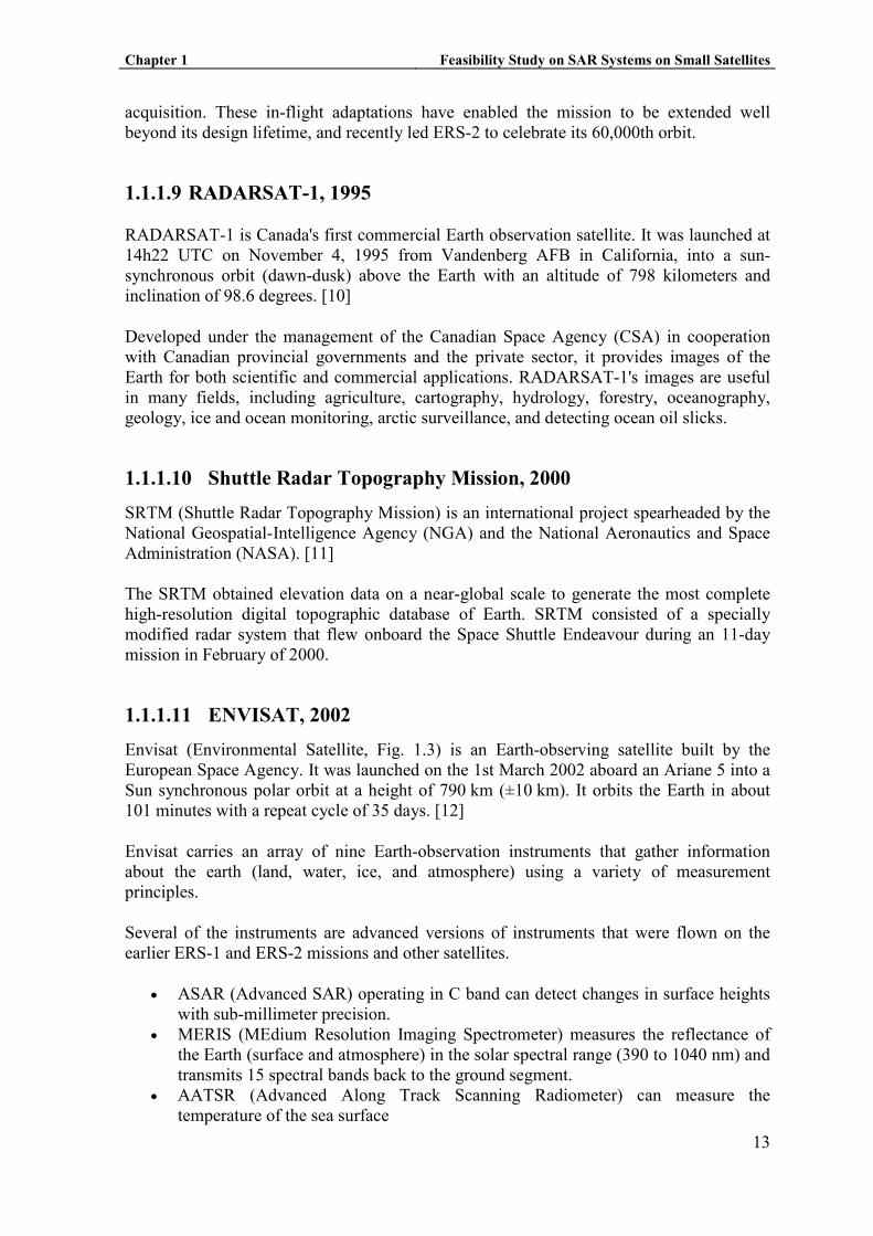
1.1.1.11 E�VISAT, 2002
Envisat (Environmental Satellite, Fig. 1.3) is an Earth-observing satellite built by the
European Space Agency. It was launched on the 1st March 2002 aboard an Ariane 5 into a
Sun synchronous polar orbit at a height of 790 km (±10 km). It orbits the Earth in about
101 minutes with a repeat cycle of 35 days. [12]
Envisat carries an array of nine Earth-observation instruments that gather information
about the earth (land, water, ice, and atmosphere) using a variety of measurement
principles.
Several of the instruments are advanced versions of instruments that were flown on the
earlier ERS-1 and ERS-2 missions and other satellites.
• ASAR (Advanced SAR) operating in C band can detect changes in surface heights
with sub-millimeter precision.
• MERIS (MEdium Resolution Imaging Spectrometer) measures the reflectance of
the Earth (surface and atmosphere) in the solar spectral range (390 to 1040 nm) and
transmits 15 spectral bands back to the ground segment.
• AATSR (Advanced Along Track Scanning Radiometer) can measure the
temperature of the sea surface
Chapter 1 Feasibility Study on SAR Systems on Small Satellites
14
• RA-2 (Radar Altimeter 2) is a dual-frequency Nadir pointing Radar operating in the
Ku band and S bands, it is used to define ocean topography, map/monitor sea ice
and measure land heights.
• MWR (Microwave Radiometer) for measuring water vapour in the atmosphere and
estimate the tropospheric delay for the Altimeter
• DORIS (Doppler Orbitography and Radiopositioning Integrated by Satellite) for
orbit determination to within 10 cm or less
• GOMOS (Global Ozone Monitoring by Occultation of Stars) looks to stars as they
descend through the Earth's atmosphere and change color, which also tells a lot
about the presence of gases such as O3 (ozone), and allows for the first time a
space-based measurement of the vertical distribution of these trace gases.
• MIPAS (Michelson Interferometer for Passive Atmospheric Sounding) is a
spectrometer
• SCIAMACHY (SCanning Imaging Absorption spectroMeter for Atmospheric
CHartographY) compares light coming from the sun to light reflected by the Earth,
which provides information on the atmosphere through which the earth-reflected
light has passed.
Fig. 1.3 Envisat during integration, 14 April 2000
Chapter 1 Feasibility Study on SAR Systems on Small Satellites
15
1.1.1.12 ALOS, 2006
Advanced Land Observation Satellite (ALOS), a Japanese satellite, was launched from
Tanegashima Island, Japan on January 24, 2006 by a H-IIA rocket. Weather and sensor
problems have caused launch delays. [13]
ALOS has been developed to contribute to the fields of mapping, precise regional land
coverage observation, disaster monitoring, and resource surveying. It enhances land
observation technologies acquired through the development and operation of its
predecessors, the Japanese Earth Resource Satellite-1 (JERS-1, or Fuyo) and the Advanced
Earth Observing Satellite (ADEOS, or Midori).
ALOS has three sensors onboard: the Panchromatic Remote-sensing Instrument for Stereo
Mapping (PRISM), which is comprised of three sets of optical systems to measure precise
land elevation; the Advanced Visible and Near Infrared Radiometer type 2 (AVNIR-2),
which observes what covers land surfaces; and the Phased Array type L-band Synthetic
Aperture Radar (PALSAR), which enables day-and-night and all-weather land observation.
1.1.1.13 TerraSAR-X, 2007
TerraSAR-X is a German remote sensing satellite program which is the first commercially
available radar satellite to offer one meter resolution [14][15].
TerraSAR-X is the first satellite ever to be built in a Public Private Partnership (PPP) in
Germany. In this partnership, the Federal Republic of Germany, represented by the
German Aerospace Center (DLR), and Europe’s leading satellite company ASTRIUM
GmbH have agreed to jointly bear the costs of constructing and implementing this X-band
radar satellite.
In order to ensure the commercial success of the mission, ASTRIUM GmbH founded its
100% subsidiary Infoterra GmbH in 2001; the company being responsible for establishing
a commercial market for TerraSAR-X data as well as TerraSAR-X-based geoinformation
products and services.
1.1.1.14 RADARSAT-2, 2007
RADARSAT-2 is an Earth observation satellite that was successfully launched December
14, 2007 for the Canadian Space Agency by Starsem, using a Soyuz FG launch vehicle,
from Kazakhstan's Baikonur Cosmodrome. RADARSAT-2 was previously assembled,
integrated and tested at the David Florida Laboratory near Ottawa, Ontario before the start
of its launch campaign. [16]
The Satellite has SAR sensor with multiple polarization modes. Its highest resolution will
be 3 m in Ultra Fine mode with 100 m positional accuracy. Its left looking capability allow
the spacecraft the unique capability to image the Antarctic on a routine basis providing
data in support of scientific research.
Chapter 1 Feasibility Study on SAR Systems on Small Satellites
16
RADARSAT-2 is based on RADARSAT-1. It has the same orbit (798 km altitude sun-
synchronous orbit with 6 p.m. ascending node and 6 a.m. descending node). RADARSAT-
2 is separated by half an orbit period (~50 min) from RADARSAT-1 (in terms of ground
track it would represent ~12 days ground track separation). It is filling a wide variety of
roles, including sea ice mapping and ship routing, iceberg detection, agricultural crop
monitoring, marine surveillance for ship and pollution detection, terrestrial defense
surveillance and target identification, geological mapping, land use mapping, wetlands
mapping, topographic mapping.
1.1.1.15 SAR-LUPE, 2007
SAR-Lupe is a SAR reconnaissance satellite imaging project of the German government,
in particular the German Ministry of Defense (BMVg) and the Federal Office of Defense
Technology and Procurement, referred to as BWB (Bundesamt für Wehrtechnik und
Beschaffung), Koblenz, Germany (BWB manages the procurement of the ground and
space segments). The overall objective is to provide high-resolution radar imagery to
German defense forces over a period of ten years starting in 2005. SAR-Lupe is in fact the
first dedicated reconnaissance satellite imaging project of Germany [17][18][19].
1.1.1.16 JianBing 5 (YaoGan WeiXing 1/3), 2007
A new satellite named Remote Sensing Satellite 1 (or YaoGan WeiXing-1 in its Chinese
translation) was successfully launched on 12 Nov 2007 by a CZ-4B (Batch-02) launch
vehicle from Taiyuan Satellite Launch Centre (TSLC). While the report about the purposes
and technical details of the satellites was very brief, it is understood that this 2,700 kg
satellite was in fact China’s first space-based SAR system, with a military designation
JianBing (JB-5) [20].
1.1.1.17 SURVEYOR, 2007
A unique and entirely commercial "Surveyor" SAR satellite constellation comprising 5
low-cost medium C Band sensors has been placed under a global design competition by the
Beijing-China sited company Tuyuan Technologies was launched in 2007 [21][22].
1.1.1.18 KOMPSAT-5, 2010
The goal of the KOMPSAT-5 (Korean Multi-purpose Satellite 5) project is to lead the
development of the first Korean SAR Satellite using manpower and facilities from the
KOMPSAT-3 program. It aims to support the national SAR satellite demand and form a
technology infrastructure to make inroads into the world space industry [23].
KOMPSAT-5, which started in the middle of 2005, will be launched in 2010 and its
payload will be an X-band SAR and it will operate at Dawn-Dusk orbit between 500km to
600km of altitude.
1.1.1.19 ASTROSAR-LITE, 2010
The AstroSAR-Lite satellite, pioneered by Astrium, provides an innovative, agile,
Chapter 1 Feasibility Study on SAR Systems on Small Satellites
17
affordable space SAR system focused to provide unprecedented revisit and coverage with
high resolution for the regional user in the tropics and sub-tropics. AstroSAR-Lite is
optimised to maritime, environmental, security and disaster monitoring applications.
The baseline satellite operates in various modes to obtain images ranging from 10 km x
1,000 km at three-metre resolution, up to 100 km x 1,000 km at 20–30 metre resolutions
over the ‘footprints’ of each of several regional users.
Mechanical steering of the whole satellite provides major beam pointing of ±45°, enabling
access to both left and right sides, augmenting and simplifying the electronic beam steering
thus minimizing cost of the expensive TR modules that are typical of other active phased
array systems.
Under a new initiative, AstroSAR-Lite customers have the option to join the AstroSAR
Lite Club – a shared constellation – effectively securing the use of several satellites for the
price of one.
1.1.1.20 SE�TI�EL,2011
The Sentinel-1 series of satellites will address the issue of data continuity for SAR data at
large. The immediate priority is to ensure such continuity for C-band data [25].
Under the current scenario, provision of ENVISAT data to feed SAR-based services is
likely to cease in the 20011-2013 timeframe. In order to meet the need for continuity, and
taking into account the availability of Radarsat-2, the first Sentinel 1 satellite should be
launched before the end of the Envisat operations.
The experience with ERS, Envisat and Radarsat constitutes the basis for the Sentinel-1
mission requirements and concept.
1.1.1.21 MAPSAR, 2013
The initiative of the joint study of a small space-borne SAR (MAPSAR) is a consequence
of a long-term Brazilian-German scientific and technical cooperation that was initiated
between INPE and DLR in the 1970s. The decision to perform a pre-phase “A” study for
MAPSAR was established in 2001 following several meetings in both agencies. Based on
the specific and complementary experience of both partners, the sharing of the thematic
responsibilities within the study was agreed. Brazil is responsible for the platform and
integrated satellite analysis and Germany for the payload and orbit analysis [26]
1.1.1.22 SAR on Proteus, launch not scheduled
PROTEUS is a French acronym standing for "Plateforme Reconfigurable pour
I'Observation, les TElecommunications et les Usages Scientifiques" (Reconfigurable
Platform for Observation, Communications and Scientific Applications) [27].
A SAR mission on the Proteus platform is being studied, the main objectives for this SAR
Chapter 1 Feasibility Study on SAR Systems on Small Satellites
18
mission concentrate in three areas:
• Accommodation due to the relatively large SAR antenna size
• Power and distribution in view of the critical requirements associated with the SAR
transmission
• Command / Control, due to the relatively large amount of data required to program the
SAR payload
1.1.1.23 SAR on Myriade, launch not scheduled
The Myrlade bus is already considered for the interferometric Cartweel (ICW’) mission
promoted by CNES. ICW aims at providing medium resolution DTM (Digital Terrain
Model) with several passive Microsar which receive the Radar echoes issued from the
transmission of a conventional SAR satellite being used as a source of opportunity. In
addition a small monostatic SAR mission is also under study [28].
1.1.2 ICC, PCOT and SARMISP
The aim of the “Institut Cartogràfic de Catalunya” (ICC), the official mapping agency of
Catalonia, is to remain in the leading edge of the mapping technologies. For a mapping
agency the benefits of satellite imagery are clear and include rapid acquisition of data
covering large areas.
The PCOT, the Catalan Earth Observation Program, is an ICC strategic program to boost
activities, products, and Earth Observation services. The aims of PCOT are:
• Promote the interest in the field of space technology in Catalonia.
• Encourage, improve and enlarge the participation of the Institute Cartographic of
Catalonia in the design, development and operation of small satellite missions for
Earth observation
• Team up with other mapping agencies doing similar projects.
• Allow public and private national end user's and stakeholders, in different fields
and at different levels, to have access to satellite information.
• Develop design methodologies and processes to translate data into useful mapping
information.
• Encourage new design ideas on satellite payload, satellite services, and satellite
constellations.
Whithin the PCOT projects, the ICC contracted a feasibility study to the Microwave
Remote Sensing group, which belongs to the Signal theory and Communications
Department of the Universitat Politècnica de Catalunya (UPC), to determine the state of
the art, main constraints and future developments in this field and to make
recommendations for a possible space-related initiative. This study is called SARMISP,
SAR Mission on Small Platforms.[29]
This final career project has been developed in the context of SARMISP and its first results
have been presented in the 2on Workshop PCOT on Radar Earth Observation.
Chapter 1 Feasibility Study on SAR Systems on Small Satellites
19
1.2 Purpose and limitations of the project
The design of an orbital SAR mission is the result of a number of trade-offs. For example,
a higher resolution requires more transmitted power, or an increase in the strip-map
azimuth resolution results in a smaller possible swath. In the following sections the most
relevant parameters of a SAR system are discussed and the inter-relation between different
parameters is explored.
It is important to emphasize right away that the most critical trade-offs are not
technological but are, instead, fundamental in nature. For example, while the transmitted
power may be increased through technological improvement, the dimensions of an
antenna, given some basic specifications, are lower bounded by first principles.
It is also worth noting that the scope of this study is limited to currently operational SAR
configurations, as the goal of this project is to evaluate the feasibility of an operational
SAR mission on a compact platform, and not to propose novel SAR concepts. Where
necessary in our analysis we have chosen the option most compatible with the nature of a
small mission. For example, within the margin of possible orbital altitudes, the lower range
is assumed since it reduces the required power.
1.3 Document Content
A brief introduction of this document contents is given next.
Chapter 2 discusses the SAR systems parameters that have to be considered in the design
of the mission. Chapter 3 presents the design flow established in order to design a SAR
mission with the parameters considered in chapter 2. Chapter 4 shows a description of the
software implemented. A SAR compact mission proposal is detailed in chapter 5.
Applications of interest, satellite orbit, sensor design and satellite down link are the main
points of the mission designed. The summary, conclusions and future lines are discussed in
chapter 6.
Chapter 2 Feasibility Study on SAR Systems on Small Satellites
20
2 SAR SYSTEM CO�SIDERATIO�S
The design of SAR system is generally dependent on the application for which it is
intended. Typically, the specifications are provided to the design engineer by the end-user
include:
• Ground range and azimuth resolution.
• Incidence angle.
• Desired swath width.
• Wavelength.
• Polarization.
• Sensitivity, which is usually expressed in as a noise equivalent 0σ .
• Radiometric accuracy; SNR.
Additional constraints are imposed by the available platform resources and overall mission
design: payload mass, available power and physical dimensions; platform altitude;
ephemeris/attitude determination accuracy; attitude control; downlink data rate, and so on.
It is worth noting that these constraints impose fundamental limitations to the achievable
performance of the resulting SAR system. For example:
• Mass and size limitations upper bound the antenna area (A) and, therefore, limit
also the antenna gain ( tG ). This has an impact on sensitivity but also on the
azimuth resolution and/or the achievable unambiguous swath.
• The maximum average radiated power (Pavg) is limited by the available DC power.
The final design is a result of an interactive procedure, trading-off conflicting requirements
to achieve the optimal design.
2.1 Orbital SAR geometry
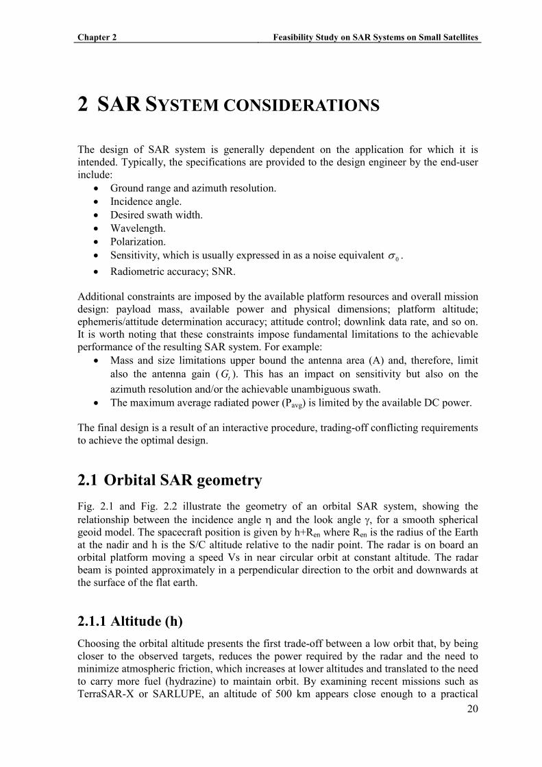
Fig. 2.1 and Fig. 2.2 illustrate the geometry of an orbital SAR system, showing the
relationship between the incidence angle η and the look angle γ, for a smooth spherical
geoid model. The spacecraft position is given by h+Ren where Ren is the radius of the Earth
at the nadir and h is the S/C altitude relative to the nadir point. The radar is on board an
orbital platform moving a speed Vs in near circular orbit at constant altitude. The radar
beam is pointed approximately in a perpendicular direction to the orbit and downwards at
the surface of the flat earth.
2.1.1 Altitude (h)
Choosing the orbital altitude presents the first trade-off between a low orbit that, by being
closer to the observed targets, reduces the power required by the radar and the need to
minimize atmospheric friction, which increases at lower altitudes and translated to the need
to carry more fuel (hydrazine) to maintain orbit. By examining recent missions such as
TerraSAR-X or SARLUPE, an altitude of 500 km appears close enough to a practical
Chapter 2 Feasibility Study on SAR Systems on Small Satellites
21
lower bound and will, therefore, be assumed throughout the rest of this chapter. As there
are missions that work in altitudes around 500 Km we will consider this altitude our
minimum altitude allowable.
The orbital velocity can be approximated by
·,t
s
t
G MV
R h=
+ (2.1)
where G is the universal gravitational constant (G ≈ 6,67428 x 10⁻¹¹
m3
kg-1
s-2
), Mt is the
Earth mass (Mt ≈ 5,9736 × 1024
kg), Rt is the Earht radius (Rt ≈ 6380 km) and h is the
satellite altitude. At 500 km height this gives an orbital velocity of approximately 7.6 km/s.
2.1.2 Incidence angle (ηηηη)
The incidence angle is the angle between the radar beam and the normal to the earth’s
surface at a particular point of interest. It is important because it affects the radar cross
section of target area (in general, a smaller incidence angle results in more backscattered
Fig. 2.1 System geometry considering a
smooth geoid.
Fig. 2.2 Simplified geometry of a side-
looking SAR
Chapter 2 Feasibility Study on SAR Systems on Small Satellites
22
power) but also the ground range resolution (which improves for larger incidence angles)
and the swath of the system.
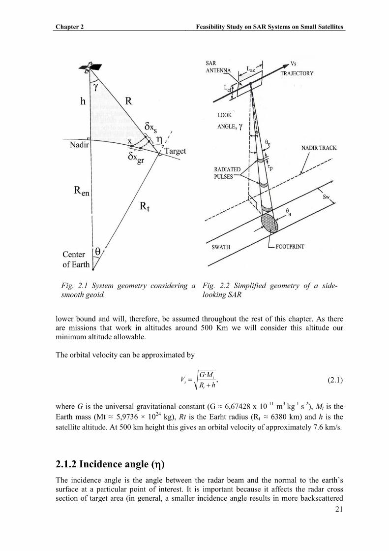
Pointing the radar beam between γmin and γmax, the system must be able to cover a given
area of interest. It is worth noting that by increasing the range of possible incidence angles
it is possible to reduce the system’s access time to any particular region of interest. The
relation between the look angle and the incidence angle is given by
( )( )sin1sin .en
t
h R
R
γη +−= (2.2)
The starting values of the look angle haven been chosen from 20º to 45º so we were able to
sight areas in 308 km with a single trace. We can calculate the range of incidence angles
and the slant range distances. Table 2.1 shows a summary of the geometric parameters
used in this report, which are further illustrated in Fig. 2.3.
2.2 Sensitivity: Radar Range Equation
One of the starting points for any radar design is the radar range equation, which relates the
signal to noise (SNR) at the receiver with the target’s radar cross-section, its distance to the
Minimum values Maximum values
γγγγ 20º 45º
ηηηη 21.64º 49.7º
R 532,13 Km 707,10 Km
Table 2.1: look angles, incidence angles and slant-range to targets
Fig. 2.3 Access region of the SAR sensor
Chapter 2 Feasibility Study on SAR Systems on Small Satellites
23
radar and a number of system parameters. The radar range equation (2.3) can be expressed
in a number of ways. For a SAR system, a useful expression is the single look signal to
noise, [30]
2 3
0 0
1 3 3,
2(4 ) ( )
ant avg t g
B sys s
P G RS=R
R k T V
η λ δ σ
π
=
(2.3)
where ηant is the radiation efficiency of the antenna, λ0 is the carrier wavelength, δRg is the
ground range resolution, σ0 is the normalized radar cross-section (radar cross-section per
area unit), R is the range to the target, kb is the Boltzmann constant, Tsys is the system
equivalent noise temperature and Vs the velocity of the platform. It is worth noting that
despite the strong dependence on the range, for orbital systems the range variation is small
in relative terms and has a smaller impact than, for example, across-swath antenna gain
variations.
The sensitivity is usually specified in terms of the noise equivalent σ0, which results from
setting SNR=1 in (2.3), which yields [31]
3 3
0, 2 3
0
2(4 ) ( ),
B sys s
ne
ant avg t g
R k T V
P G R
πσ
η λ δ
=
(2.4)
The sensitivity can be improved in several ways:
1. Increase the average power by increasing either the peak power, which is
technology-limited, or the pulse duration. It is upper-bounded by the total available
power.
2. Reduce the range to the target, which for an orbital case implies lowering the
orbital altitude.
3. Increase the antenna gain, which implies increasing it physical size and either
degrading the azimuth resolution or the swath width.
4. Reduce the required resolution.
5. Reduce the noise introduced by the system (either receiver noise or quantization
noise). It is worth stressing that the noise power is lower bounded by the noise
temperature of the antenna, which for a SAR system is usually in the order of
300K.
6. Reduce system losses by improving the antenna feed system (waveguide) or by
inserting T/R modules into the feed to improve the system gain; again at the cost of
increasing power consumption.
2.3 Resolution considerations.
2.3.1 Range Resolution
For a SAR system, the ground range resolution is given by [32]
,
2 sing
R
cR
Bδ
η= (2.5)

Chapter 2 Feasibility Study on SAR Systems on Small Satellites
24
where BR is the radar pulse bandwidth and η is the incidence angle. Within legal (In the
government web [33] the bandwidth limits for space earth observation are detailed) and
technological limitations, the range resolution can be made arbitrarily fine by increasing
the pulse bandwidth at the cost of loosing sensitivity. The resolution also improves for
increasing incidence angles, but this also increases the range and tends to reduce the
normalized radar cross-section. The relation between slant range and ground range
resolution is illustrated in Fig. 2.4.
2.3.2 Azimuth Resolution
The azimuth resolution limit of a SAR system is approximately given by
,
2
azLxδ ≥ (2.6)
where Laz is the azimuth dimension of the antenna. This expression results from
approximating the beam-width by θH = λ/Laz. The exact expression depends on the exact
beam-pattern and on how the SAR processing is implemented. Exists the possibility to
improve the along-track resolution ∆x it is necessary to decrease the antenna length in the
along-track dimension.
2.4 The Antenna
The SAR antenna assembly typically consists of either a single high gain used for both
transmit and receive consisting of a feed system or by an array of transmit/receive
elements, usually organized in tiles. The key antenna parameters affecting the SAR
performance are the antenna gain (or directivity) and its beam pattern. The antenna gain is
directly proportional to its effective area (Aef). The gain is given by the product of the
Fig. 2.4: Radar geometry illustrating the ground swath and θV

Chapter 2 Feasibility Study on SAR Systems on Small Satellites
25
antenna efficiency and its directivity D:
2 2
44 efaAA
G Dππ
η ηλ λ
= = = . (2.7)
The antenna efficiency is given by the product of the radiation efficiency (which depends
on resistive losses) and the aperture efficiency, which depends on the illumination.
Typically, to achieve the desired sensitivity for space-borne systems, aperture gains well
over 30 dB or more are required.
2.4.1 Minimum antenna area (zero order ambiguity analysis)
A first lower bound on the required antenna (effective) area can be derived from a zero
order analysis of range-azimuth ambiguities. For a given antenna length, which as seen in
(2.6) is approximately twice the azimuth, a minimum PRF can be immediately derived.
This can be done in several ways, but the simplest reasoning is that for each independent
sample in azimuth in the output image the system must acquire, at least, one raw sample.
Thus, a SAR system should transmit, at least, one pulse every time it advances a distance
of Laz/2 and the minimum PRF is, therefore
min
2 s
az
VPRF
L= . (2.8)
This minimum PRF sets a maximum unambiguous slant-range swath
slant,max
min
·swath
2· 4·
az
s
c Lc
PRF V= = , (2.9)
Which projected onto ground range gives a maximum swath of
max
·swath
4· sin
a
s
c L
V θ= . (2.10)
To avoid out of swath targets to produce significant ambiguous echoes, their signal must be
suppressed by the radiation pattern in elevation of the antenna. In other words, the foot-
print of the antenna must be smaller than the maximum swath. Combining the expression
of this footprint with (2.10) yields
4· tanseff
VA
c
λ θ≥ . (2.11)
This expression gives the minimum area of a SAR antenna given the carrier wavelength,
the incidence angle, and the orbital velocity, which is set by the orbital height and almost
constant for the range of useful orbital altitudes. It is noteworthy that this minimum area is
independent of other requirements, such as sensitivity or resolution.
For every band we will have different minimum antenna areas, as it is shown in Fig. 2.5.
It is worth noting that this minimum antenna area results from a zero order analysis, in

Chapter 2 Feasibility Study on SAR Systems on Small Satellites
26
which it is assumed that the PRF must satisfy the Nyquist minimum sapling rate. It is
worth noting that, strictly speaking, it is possible, to some extent, to operate with sub-
Nyquist PRF values by reducing the effective Doppler bandwidth, which results in a loss of
azimuth resolution. However, the condition given in (2.11) is both widely assumed in the
literature and satisfied by all existing SAR missions.
2.5 Ambiguity Analysis
In section 2.4.1 a zero order ambiguity analysis was presented. In this analysis it was
assumed that to reject ambiguous radar echoes corresponding to out of swath target it is
necessary that the swath be smaller than the footprint of the antenna pattern on the ground.
However, the size of this footprint was implicitly given in terms of the one-way 3 dB
beamwidth, which for a uniform antenna illumination in elevation is given by
,3H dB
HL
λθ = . (2.12)
This criterion would only provide 6dB suppression for ambiguous targets located at the
edges of the footprint. Considering the large dynamic range of σ0, it is obvious that this
suppression is insufficient. The existence of range ambiguities caused by the antenna
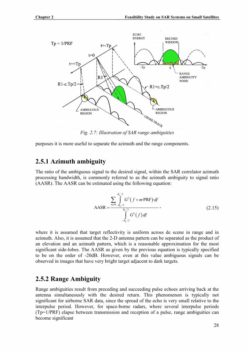
pattern elevation side-lobes is illustrated in Fig. 2.7.
Likewise, the expression for the minimum PRF given in (2.8) can be related to the need to
sample the Doppler spectrum at least at the Nyquist rate (twice the Doppler bandwidth).
Here the Doppler bandwidth is determined by the antenna beam-width in the azimuth
direction. Expression (2.8) corresponds to the Nyquist rate considering the 6dB Doppler
bandwidth, which does not prevent spectral components corresponding to the side-lobes of
the antenna pattern to alias back into the main part of the spectrum, which result in azimuth
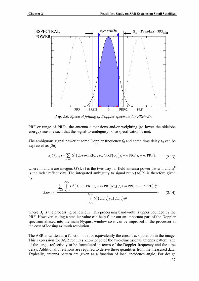
ambiguities. This spectral folding is illustrated in Fig. 2.6.
For a given range and azimuth antenna pattern, the PRF must be selected such that the total
ambiguity noise contribution is very small relatively to the signal. Alternatively, given a
Fig. 2.5 Minimum required antenna area for LEO SAR system at different
frequency bands.
Chapter 2 Feasibility Study on SAR Systems on Small Satellites
27
PRF or range of PRFs, the antenna dimensions and/or weighting (to lower the sidelobe
energy) must be such that the signal-to-ambiguity noise specification is met.
The ambiguous signal power at some Doppler frequency f0 and some time delay τ0 can be
expressed as [36]
( ) ( )2
0 0 0 0 0 0 0
, 0
( , ) ·PRF, / PRF · ·PRF, / PRFa
m n
S f G f m n f m nτ τ σ τ≠
= + + + +∑ , (2.13)
where m and n are integers G2(f, τ) is the two-way far field antenna power pattern, and σ0
is the radar reflectivity. The integrated ambiguity to signal ratio (ASR) is therefore given
by
( ) ( )
( ) ( )
/ 2
2
0 0 0 0 0
, 0 / 2
/ 2
2
0 0 0 0 0
/ 2
·PRF, / PRF · ·PRF, / PRF
( )
, · ,
p
p
p
p
B
m n B
B
B
G f m n f m n df
ASR
G f f df
τ σ τ
τ
τ σ τ
≠ −
−
+ + + +
=
∑ ∫
∫
, (2.14)
where Bp is the processing bandwidth. This processing bandwidth is upper bounded by the
PRF. However, taking a smaller value can help filter out an important part of the Doppler
spectrum aliased into the main Nyquist window so it can be improved in the processor at
the cost of loosing azimuth resolution.
The ASR is written as a function of τ, or equivalently the cross-track position in the image.
This expression for ASR requires knowledge of the two-dimensional antenna pattern, and
of the target reflectivity to be formulated in terms of the Doppler frequency and the time
delay. Additionally relations are required to derive these quantities from the measured data.
Typically, antenna pattern are given as a function of local incidence angle. For design
Fig. 2.6: Spectral folding of Doppler spectrum for PRF=BD
Chapter 2 Feasibility Study on SAR Systems on Small Satellites
28
purposes it is more useful to separate the azimuth and the range components.
2.5.1 Azimuth ambiguity
The ratio of the ambiguous signal to the desired signal, within the SAR correlator azimuth
processing bandwidth, is commonly referred to as the azimuth ambiguity to signal ratio
(AASR). The AASR can be estimated using the following equation:
( )
( )
/ 2
2
0 / 2
/ 2
2
/ 2
·PRF ·
AASR
p
p
p
p
B
m B
B
B
G f m df
G f df
≠ −
−
+
=
∑ ∫
∫
, (2.15)
where it is assumed that target reflectivity is uniform across de scene in range and in
azimuth. Also, it is assumed that the 2-D antenna pattern can be separated as the product of
an elevation and an azimuth pattern, which is a reasonable approximation for the most
significant side-lobes. The AASR as given by the previous equation is typically specified
to be on the order of -20dB. However, even at this value ambiguous signals can be
observed in images that have very bright target adjacent to dark targets.
2.5.2 Range Ambiguity
Range ambiguities result from preceding and succeeding pulse echoes arriving back at the
antenna simultaneously with the desired return. This phenomenon is typically not
significant for airborne SAR data, since the spread of the echo is very small relative to the
interpulse period. However, for space-borne radars, where several interpulse periods
(Tp=1/PRF) elapse between transmission and reception of a pulse, range ambiguities can
become significant
Fig. 2.7: Illustration of SAR range ambiguities
Chapter 2 Feasibility Study on SAR Systems on Small Satellites
29
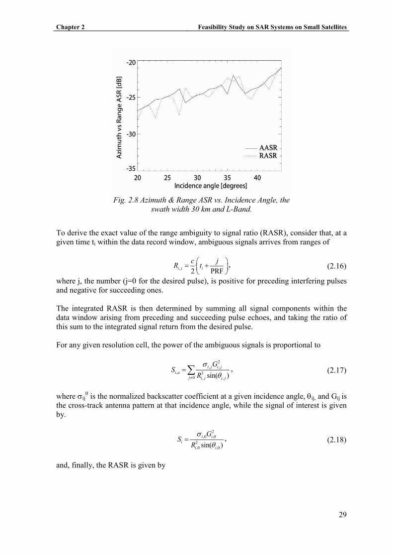
Fig. 2.8 Azimuth & Range ASR vs. Incidence Angle, the
swath width 30 km and L-Band.
To derive the exact value of the range ambiguity to signal ratio (RASR), consider that, at a
given time ti within the data record window, ambiguous signals arrives from ranges of
, ·
2 PRFi j i
c jR t
= +
, (2.16)
where j, the number (j=0 for the desired pulse), is positive for preceding interfering pulses
and negative for succeeding ones.
The integrated RASR is then determined by summing all signal components within the
data window arising from preceding and succeeding pulse echoes, and taking the ratio of
this sum to the integrated signal return from the desired pulse.
For any given resolution cell, the power of the ambiguous signals is proportional to
2
, ,
, 30 , ,sin( )
i j i j
i a
j i j i j
GS
R
σ
θ≠
= ∑ , (2.17)
where σij0 is the normalized backscatter coefficient at a given incidence angle, θij, and Gij is
the cross-track antenna pattern at that incidence angle, while the signal of interest is given
by.
2
,0 ,0
3
,0 ,0sin( )
i i
i
i i
GS
R
σθ
= , (2.18)
and, finally, the RASR is given by
Chapter 2 Feasibility Study on SAR Systems on Small Satellites
30
,
RASRi
i
i a
i
S
S=
∑∑
, (2.19)
the average ratio between signal of interest and ambiguous signal levels.
2.6 PRF Selection.
The set of values that the PRF can assume is constrained by a number of other factors. The
preceding discussions on azimuth and range ambiguities, the AASR and RASR are both
highly dependent on the selection of PRF. Its selection is further constrained for a SAR
system that has a single antenna for both transmit and receive. Considering that ina a
space-borne, at any given time, there are a number of pulses in the air, the transmitted
pulses must be interspersed with the data reception. Additionally, the PRF must be selected
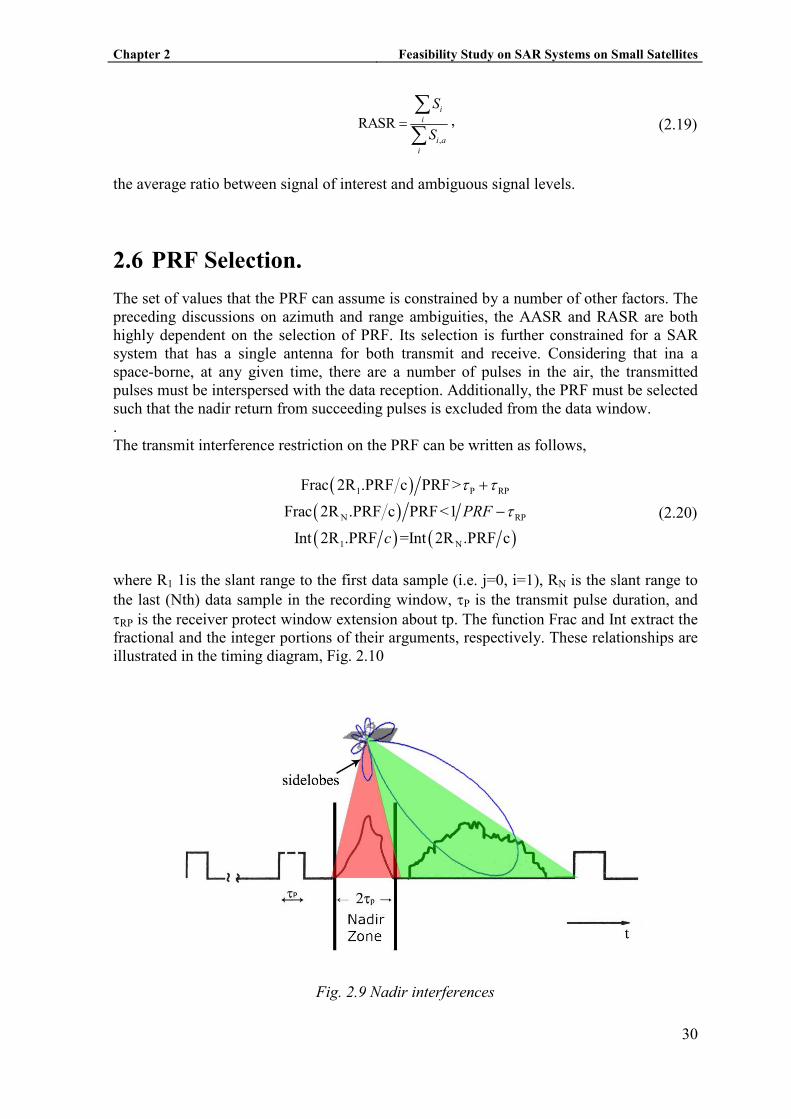
such that the nadir return from succeeding pulses is excluded from the data window.
.
The transmit interference restriction on the PRF can be written as follows,
( )1 P RPFrac 2R .PRF c PRF>τ τ+
( )N RPFrac 2R .PRF c PRF<1 PRF τ−
( ) ( )1 NInt 2R .PRF =Int 2R .PRF cc
(2.20)
where R1 1is the slant range to the first data sample (i.e. j=0, i=1), RN is the slant range to
the last (Nth) data sample in the recording window, τP is the transmit pulse duration, and
τRP is the receiver protect window extension about tp. The function Frac and Int extract the
fractional and the integer portions of their arguments, respectively. These relationships are
illustrated in the timing diagram, Fig. 2.10
Fig. 2.9 =adir interferences

Chapter 2 Feasibility Study on SAR Systems on Small Satellites
31
The nadir interference restriction on the PRF can be written as follows:
N
p 1
2h c + j PRF> 2R
2h c +2 + j PRF < 2R
c
cτ j=0,±1, ±2,…,±,nh (2.21)
where H ≅ Rs-Rt is the sensor altitude above the surface nadir point. We have assumed in
the above analysis that the duration of the nadir return is 2τp. The actual nadir return
duration will depend on the characteristics of the terrain. For rough terrain the significant
nadir return could be shorter or longer than 2τp. An example is given in Fig. 2.9.
Then, the range of PRFs values is established by the maximum acceptable range and
azimuth ambiguity-to-signal ratios, as well as the transmit and nadir interference. At some
look angles, there may be no acceptable PRFs that achieve the minimum requirements. In
general, as the off-nadir angle is increased, the PRF availability is reduced and the
ambiguity requirements must be lowered to find acceptable PRFs.
Fig. 2.11 PRF against η illustrating excluded zones as
a result of transmit and nadir interference. We have
considered a 30 Km swath width.
Fig. 2.10 Transmit interferences
Chapter 2 Feasibility Study on SAR Systems on Small Satellites
32
2.7 Signal Parameters (f0, ττττ0, polarization)
The radar transmits a waveform s(t) which is backscattered by a target at range R, so that
the echo corresponding to that target arrives with a time-delay τ = 2R/c. The energy of the
input signal is just
,S PE P τ= (2.22)
where τp is the duration of the pulse and Ps is the average power this duration (which for
chirp signals is also the peak power). Long pulses of tolerable average power can be used
to obtain large energy satisfying the detectability requirements, while at the same time a
wide bandwidth can be used to obtain good resolution.
2.7.1 Frequency Band
A fundamental system parameter is the center frequency of the system. Its choice depends
on the applications, the required resolution, and on technological aspects. In this study we
have considered three possible bands: L-band, C-band and X-band. Lower frequencies (P-
band) have been excluded from the start because of the large dimensions of the required
antennas. Higher frequencies have been discarded because of the intrinsic technological
difficulty associated to them.
At L-band, the longer wavelengths are appropriate for missions that require a larger degree
of penetration, for example for detection and imaging of soil moisture, or for retrieval of
biomass. Because the available bandwidth, both from a technological and from a legal
point of view, scales with frequency, this increased penetration goes at the expense of
resolution.
Moving to the high frequency end, X-band (10 GHz) is the preferred option for high
resolution systems. This is due the availability of large bandwidths (for example,
TerraSAR-X uses up to 300 MHz bandwidth) and the technological maturity of space
ready X-band components. Also, at higher frequencies the antenna area is smaller for a
given antenna gain, which enables the design of more compact systems.
The C-Band (typically around 5.4 GHz) is a compromise between the two extremes,
offering reasonable performance in terms of resolution and surface penetration. For the
past 15 years C-Band was the preferred choice for some very well performing SAR
systems like for the ESA missions ERS-1, -2 and ENVISAT due to the technological
availability at the time of system definition and in order to maintain data continuity over a
long period. All three missions are part of the strong Astrium GmbH SAR heritage basis,
due to its role as prime contractor, mission prime and SAR subsystem supplier.
2.7.2 Bandwidth and pulse duration.
The slant-range resolution of a SAR system is given by the two-way speed of light divided
by the transmitted pulse bandwidth,
Chapter 2 Feasibility Study on SAR Systems on Small Satellites
33
.
2 R
cR
Bδ = (2.23)
Using a chirp signal, the required bandwidth is achieved using a frequency modulated
signal, where the frequency varies linearly over the duration (τp). By increasing the pulse
duration (decreasing the chirp rate) higher energy pulses can be obtained with a reasonable
peak power (which is a technological limitation), as expressed by (2.22).
During the time that a given target is observed by a SAR system the corresponding echoes
are first received with a positive Doppler frequency shift, while the system is approaching
the target, which decreases until a maximum negative Doppler shift when the target exits
the radar beam. This Doppler shift distorts the received signal. In the case of a chirp signal,
this distortion introduces an apparent range shift, which is more severe for lower chirp
rates. This apparent shift should be small compared to the range resolution. This
considering the Doppler bandwidth, this condition can be expressed as
,
2
azp
s
L
Vτ ≪ (2.24)
where Laz is the length of the SAR antenna. This is well satisfied for current space systems.
2.7.3 Polarization.
SAR systems, like most radar systems, can be designed to operate either in a single
polarization mode, usually transmitting and receiving in the same linear polarization, or
designed to operate in a number of polarimetric modes:
1. Light polarimetry: in this mode the system transmits in a fixed polarization (which
can be linear or circular) and receives in two orthogonal polarizations. For example,
the system may transmit in vertical polarization and receive in both vertical and
horizontal, in which case the two channels are typically identified as VV and HV.
Light polarimetry is useful for some applications and does not imply any significant
fundamental trade-off. It does, however, increase the technological complexity of
the system and, everything else equal, it duplicates the data rate and downlink
bandwidth requirements.
2. Alternating polarization: in this mode (implemented, for example, in ENVISAT),
the system sends a number of pulses in one polarization, receiving in both
polarizations, followed by another series of pulses in the orthogonal polarization.
System considerations are the same as in the case of light polarimetry, except for
the fact that the azimuth resolution is degraded by at least a factor of two.
3. Full polarimetry: in this mode the system alternates pulses in both polarizations. In
contrast to the other modes, the implementation of this mode has an impact on a
number of design trade-offs.
Chapter 3 Feasibility Study on SAR Systems on Small Satellites
34
3 SAR SYSTEM TRADE-OFFS A�D DESIG�
FLOW
Taking into account the trade-offs between SAR parameters discussed in previous sections,
we have generated an orbital SAR mission design. This design flow corresponds to a
standard strip-map mode. Due to the limited scope of this study only first order
optimizations have been done.
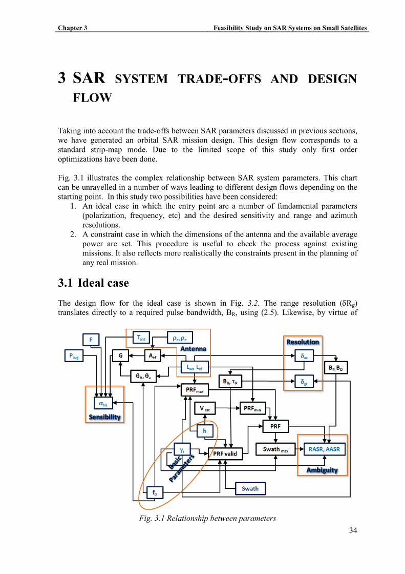
Fig. 3.1 illustrates the complex relationship between SAR system parameters. This chart
can be unravelled in a number of ways leading to different design flows depending on the
starting point. In this study two possibilities have been considered:
1. An ideal case in which the entry point are a number of fundamental parameters
(polarization, frequency, etc) and the desired sensitivity and range and azimuth
resolutions.
2. A constraint case in which the dimensions of the antenna and the available average
power are set. This procedure is useful to check the process against existing
missions. It also reflects more realistically the constraints present in the planning of
any real mission.
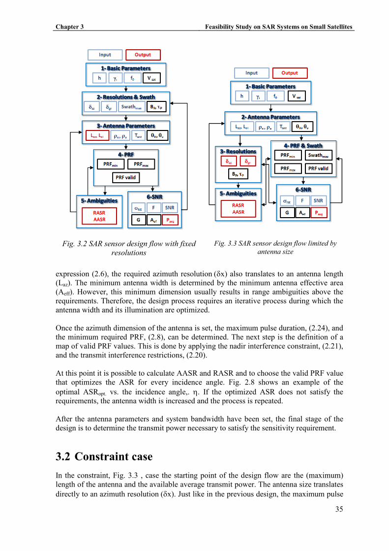
3.1 Ideal case
The design flow for the ideal case is shown in Fig. 3.2. The range resolution (δRg)
translates directly to a required pulse bandwidth, BR, using (2.5). Likewise, by virtue of
Fig. 3.1 Relationship between parameters
Chapter 3 Feasibility Study on SAR Systems on Small Satellites
35
expression (2.6), the required azimuth resolution (δx) also translates to an antenna length
(Laz). The minimum antenna width is determined by the minimum antenna effective area
(Aeff). However, this minimum dimension usually results in range ambiguities above the
requirements. Therefore, the design process requires an iterative process during which the
antenna width and its illumination are optimized.
Once the azimuth dimension of the antenna is set, the maximum pulse duration, (2.24), and
the minimum required PRF, (2.8), can be determined. The next step is the definition of a
map of valid PRF values. This is done by applying the nadir interference constraint, (2.21),
and the transmit interference restrictions, (2.20).
At this point it is possible to calculate AASR and RASR and to choose the valid PRF value
that optimizes the ASR for every incidence angle. Fig. 2.8 shows an example of the
optimal ASRopt. vs. the incidence angle,. η. If the optimized ASR does not satisfy the
requirements, the antenna width is increased and the process is repeated.
After the antenna parameters and system bandwidth have been set, the final stage of the
design is to determine the transmit power necessary to satisfy the sensitivity requirement.
3.2 Constraint case
In the constraint, Fig. 3.3 , case the starting point of the design flow are the (maximum)
length of the antenna and the available average transmit power. The antenna size translates
directly to an azimuth resolution (δx). Just like in the previous design, the maximum pulse
Fig. 3.2 SAR sensor design flow with fixed
resolutions
Fig. 3.3 SAR sensor design flow limited by
antenna size
Chapter 3 Feasibility Study on SAR Systems on Small Satellites
36
duration (2.24), the minimum PRF allowed (2.8), the maximum swath reachable (2.10) and
the valid PRF values are determined.
To obtain the required AASR and RASR, the antenna width and optimum values are
iteratively adjusted. The difference is that the antenna is not optimized for the ASR level,
because initially it can be wider than it needs to be. On the other hand, with wider antenna
values we can relax more the PRF conditions if the ASR level is far from -20dB.
The final stage is calculating the transmit power required to get the range resolution for a
specified sensitivity. For a fixed transmit power, a higher sensitivity can be attained by
decreasing the signal bandwidth at the cost of range resolution (2.5). More resolution
required proportionally more power.
3.3 Design Flow Validation: TerraSAR-X “revisited”
Trying to validate our design methodology we have tested the design flows considered in
this chapter. In order to validate the process, first main parameters of the TerraSAR-X
mission have been set as constraints in order to try to reproduce its final specifications.
This exercise is also useful to evaluate how tight the design of TerraSAR-X is.
The objective is to obtain a similar system as the actual TerraSAR-X, starting from its
mission parameters, which are listed in Table 3.1.
The minimum antenna area has been calculated using (2.11) and represented, as a function
of the incidence angle in Fig. 3.4. This yields a minimum area of 0.69 m2
for a 20º
incidence angle and 2.95 m2
for a 45º incidence angle. This latest figure would, therefore,
set the lower bound for the antenna area, without taking into account the ambiguity
requirements.
TerraSAR-X nominal strip-map azimuth resolution is 3 m, for which the optimal antenna
length is about 6 m. TerraSAR-X actual antenna length is around 4,8 m, which implies
that, the azimuth resolution have been relaxed in order to meet ASR requirements. For this
reason, a significant fraction of the Doppler Bandwidth is being filtered-out. this length and
the previously obtained minimum area, the minimum antenna width is 0.5 m.
Following the design flow, the valid PRF values are calculated and illustrated in Fig. 3.5.
Then, for each incidence angle the design procedure checks if there is a valid PRF that
gives the desired ASR for the desired 30 Km swath. If this condition is not achieved the
antenna width is and the process is repeated. In this particular case, the ASR requirements
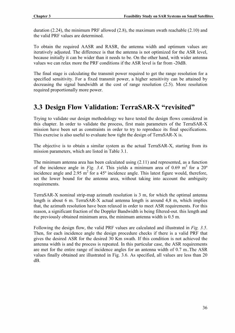
are met for the entire range of incidence angles for an antenna width of 0.7 m..The ASR
values finally obtained are illustrated in Fig. 3.6. As specified, all values are less than 20
dB.

Chapter 3 Feasibility Study on SAR Systems on Small Satellites
37
In order to calculate the AASR it has been assumed that the illumination of the antenna,
like in most orbital missions, is uniform in azimuth. In practice it found that an azimuth
tapering does not improve the AASR levels while reducing the antenna gain. In range
however, the RASR depends significantly on the tapering in elevation of the antenna. This
tapering is optimized, in terms of SNR and ASR for each operating mode of the system. In
our model this optimization has been limited to choosing between no tapering, which
works best for large incidence angles, and a Hanning tapering, which works best for small
incidence angles (see Fig. 3.7).
Incidence dependent tapering requires a relatively complex active antenna, like that of
ENVISAT’s ASAR and TerraSAR-X, which is also required for electronic steering in
elevation (in contrast to mechanical steering accomplished by rotating the platform). It is,
therefore, unclear that it is a viable solution for a compact, low-cost, mission.
Fig. 3.4 TerraSAR-X: Mínimum antenna area Fig. 3.5 TerraSAR-X: non interference
PRF values
f0 9.65 GHz (X-Band)
Orbital altitude 514 Km.
Incidence angle between 20º and 45º
Resolutions δRg= 1’7m
δx= 3 m
Swath 30 Km
σ0 -20 dB
ASR 20 dB
Mode Strip-map
Polarization single
Table 3.1 TerraSAR-X mission parameters
Chapter 3 Feasibility Study on SAR Systems on Small Satellites
38
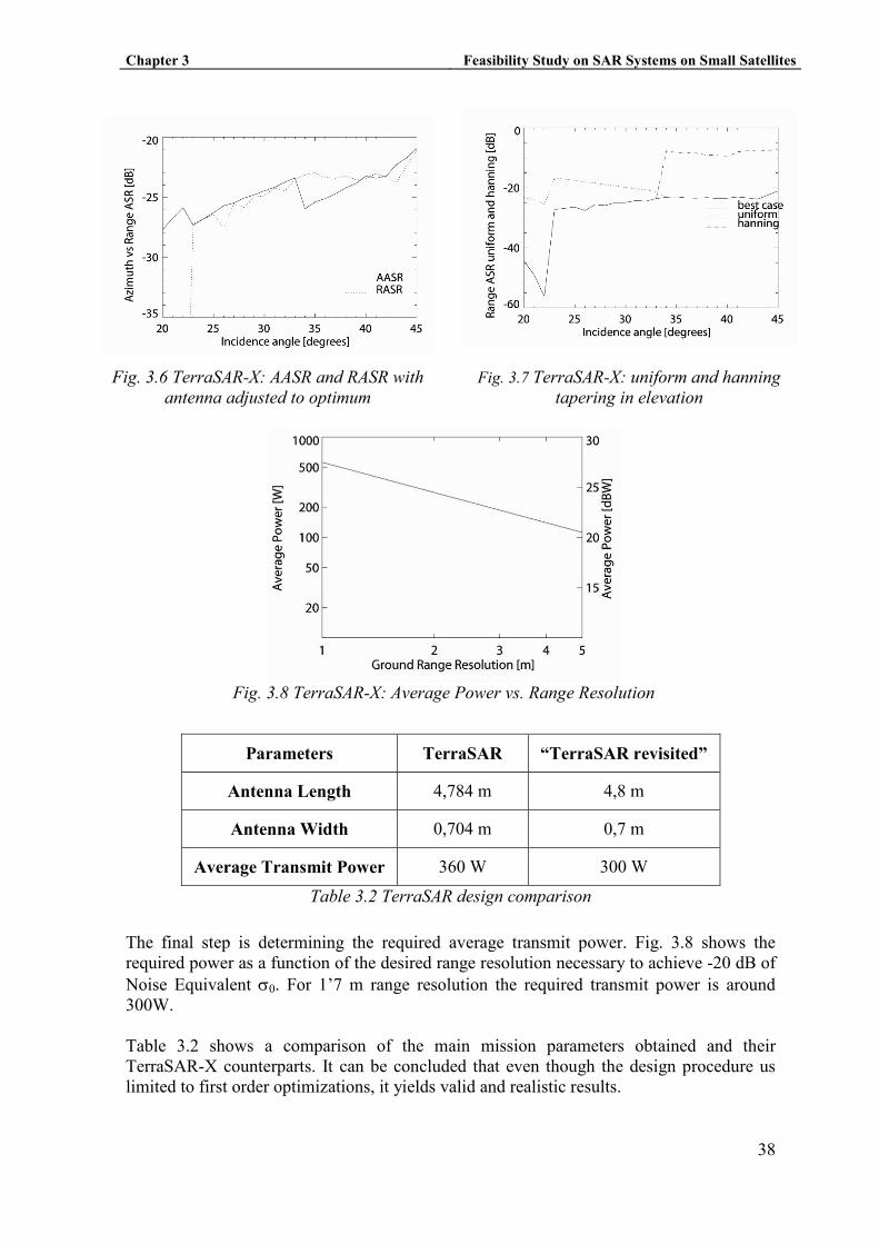
The final step is determining the required average transmit power. Fig. 3.8 shows the
required power as a function of the desired range resolution necessary to achieve -20 dB of
Noise Equivalent σ0. For 1’7 m range resolution the required transmit power is around
300W.
Table 3.2 shows a comparison of the main mission parameters obtained and their
TerraSAR-X counterparts. It can be concluded that even though the design procedure us
limited to first order optimizations, it yields valid and realistic results.
Fig. 3.6 TerraSAR-X: AASR and RASR with
antenna adjusted to optimum
Fig. 3.7 TerraSAR-X: uniform and hanning
tapering in elevation
Fig. 3.8 TerraSAR-X: Average Power vs. Range Resolution
Parameters TerraSAR “TerraSAR revisited”
Antenna Length 4,784 m 4,8 m
Antenna Width 0,704 m 0,7 m
Average Transmit Power 360 W 300 W
Table 3.2 TerraSAR design comparison
Chapter 4 Feasibility Study on SAR Systems on Small Satellites
39
4 S3D BETA VERSIO� (SOFTWARE FOR SAR
SE�SOR DESIG�)
The S3D can be divided in 2 parts. The front-end is the interface that allows the user to
introduce the parameters and see the results. The back-end is made up by a list of routines
that are called by the front-end.
4.1 IDL Introduction
The language used in the implementation of the S3D is IDL (Interactive Data Language).
IDL is a complete data analysis and visualization environment that is used in a wide range
of science and engineering disciplines for processing and analyzing numerical and image
data. It is often used in advanced science/technical courses. IDL integrates an array-
oriented language with numerous mathematical analysis and graphical display techniques,
thus giving you more flexibility than other mathematical languages.
4.2 S3D Back-end description
A list of routines and functions, 64 has been programmed in order to turn the mathematical
equations described in chapter 2 into processes that allow us to design the sensor.
In order to understand the capabilities of the software, a brief description of the most
relevant routine follows.
• mysar: Creates a structure with the parameters of the SAR mission.
• orbit_vel: Calculates the satellite velocity as shown in equation (2.1)
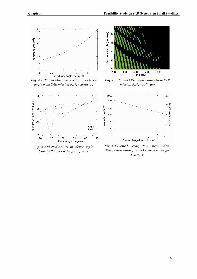
• areamin: Based on the theory explained in chapter 2.4.1, it calculates the lower
bound on the required antenna (effective) area from a zero order analysis of range-
azimuth ambiguities. It establishes the starting point of the antenna. The plotted
result is shown on Fig. 4.2.
• PRFbad: Based on the theory explained in chapter 2.6, it calculates the PRF valid
values. Optionally, it visualizes these valid PRF values for a range of incidence
angles, as seen in Fig. 4.3
• sarsens: Using Radar equation (chapter 2.2) it is easy to find a relation between the
Average Power and the Range Resolution. The use of the plot, Fig. 4.5, could be
very useful in the constraint case in which the range resolution could be adjusted to
establish a reasonable Average Power.
• saramb: This function calculates the Range and Azimuth ambiguities as explained
in section 2.5. The values of ASR are given for one concrete incidence angle, PRF,
antenna size and illumination tapering.

Chapter 4 Feasibility Study on SAR Systems on Small Satellites
40
• bestPRF: This function iterates saramb in order to find the PRF value that achieves
the best ASR rejection for every incidence angle. The ASR results can be plotted as
showed in Fig. 4.4
• bestLel: Starting from the minimum antenna width, it iterates bestPRF in order to
find the minimum width that satisfies the ASR requirements for every incidence
angle.
4.3 S3D Front-end description
The S3D front-end consists in 3 graphic user interfaces (GUI) based on the 2 design flow
cases described in chapter 3. The first one is only to choose the mission design flow, Fig.
4.1. The Ideal Case GUI, Fig. 4.6, shows the steps to follow in case the mission has
resolution requirements and freedom antenna size. Finally, the Constraint Case GUI, Fig.
4.7, follows the design flow in which the mission has to be built from an antenna specific
size. Every button of the GUI executes an IDL routine from the required action. Input and
output parameters for ideal and constraint case are listed.
• Ideal Case. Input parameters: SAR Mission Version, Sigma Noise, Ambiguity
Signal Ratio, Satellite altitude, Incidence Angle Range, Frequency, Pulse Time,
Azimuth Resolution, Range Resolution, Swath, PRF Range and Aperture
Efficiency.
• Ideal Case. Output parameters: PRF Valid values, Antenna Length, Antenna Width,
Average Power Required, ASR values.
• Constraint Case. Input parameters: SAR Mission Version, Sigma Noise, Ambiguity
Signal Ratio, Satellite altitude, Incidence Angle Range, Frequency, Pulse Time,
Antenna Length, Antenna Width, Aperture Efficiency, Range Resolution, Swath
and PRF Range.
• Constraint Case. Output parameters: PRF Valid values, Azimuth Resolution,
Average Power Required, ASR values.
In order to reduce the process time, improvements in the implementation of the algorithms
can be done. This is a preliminary version and more features can be added.
Fig. 4.1 Design Flow Selection GUI
Chapter 4 Feasibility Study on SAR Systems on Small Satellites
41
Fig. 4.2 Plotted Minimum Area vs. incidence
angle from SAR mission design Software
Fig. 4.3 Plotted PRF Valid Values from SAR
mission design software
Fig. 4.4 Plotted ASR vs. incidence angle
from SAR mission design software
Fig. 4.5 Plotted Average Power Required vs.
Range Resolution from SAR mission design
software
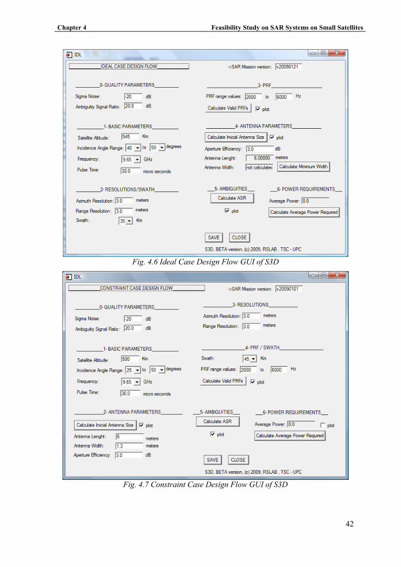
Chapter 4 Feasibility Study on SAR Systems on Small Satellites
42
Fig. 4.7 Constraint Case Design Flow GUI of S3D
Fig. 4.6 Ideal Case Design Flow GUI of S3D
Chapter 5 Feasibility Study on SAR Systems on Small Satellites
43
5 COMPACT MISSIO� DESIG� PROPOSAL
In this chapter the theory and procedures discussed in the previous chapters is applied to
the design a compact SAR mission. In order to set a context for the mission, operational
SAR applications are explained. Then a proposal of a possible SAR sensor is presented.
5.1 Applications of interest
This chapter contains a review of the main applications of the SAR technology. It is worth
mentioning that the level of maturity of the applications presented in this chapter must be
understood in the framework of the existing SAR systems.
For instance, most of the applications have been tested and analyzed at C-band, as data
were available from the ERS-1/2 and the ASAR-ENVISAT missions. The validity of these
applications at other bands, as for instance X-band, will be determined in the future thanks
to the recent launch of the TerraSAR system.
5.1.1 Agriculture
L or C band are the recommended bands in which a SAR system has to be focused on.
Nevertheless, an X-band system could be also exploited for this type of applications,
especially when the quantitative retrieval of plant parameters is the objective. L- or C-band
systems perform well when classification is the main issue [37].
Agriculture applications are feasible and clearly promising if polarimetric data are
available. The physical reason behind this statement is that polarimetry makes data
sensitive to the internal structure of the plant. This sensitivity cannot be achieved with non
polarimetric SAR data. Other sources of diversity as multitime or multifrequency improve
the retrieval of information.
High spatial resolution data are desirable as they make possible precision farming (Fig.
5.1), in order to retrieve internal information and inhomogeneities of single agricultural
fields.
One of the most appealing features of remote sensing for the final precision farming users
is the possibility to monitor the crops in time, that is, to perform multi-time acquisitions. In
general weekly information could fulfill the needs of the final users.
5.1.2 Forestry
Forests are a very important part of the Earth cover and its study, in terms of National
Forest Inventories, is important for both national and commercial agents [38]. The
complexity of the forest cover compromises, in part, the possibility to perform an accurate
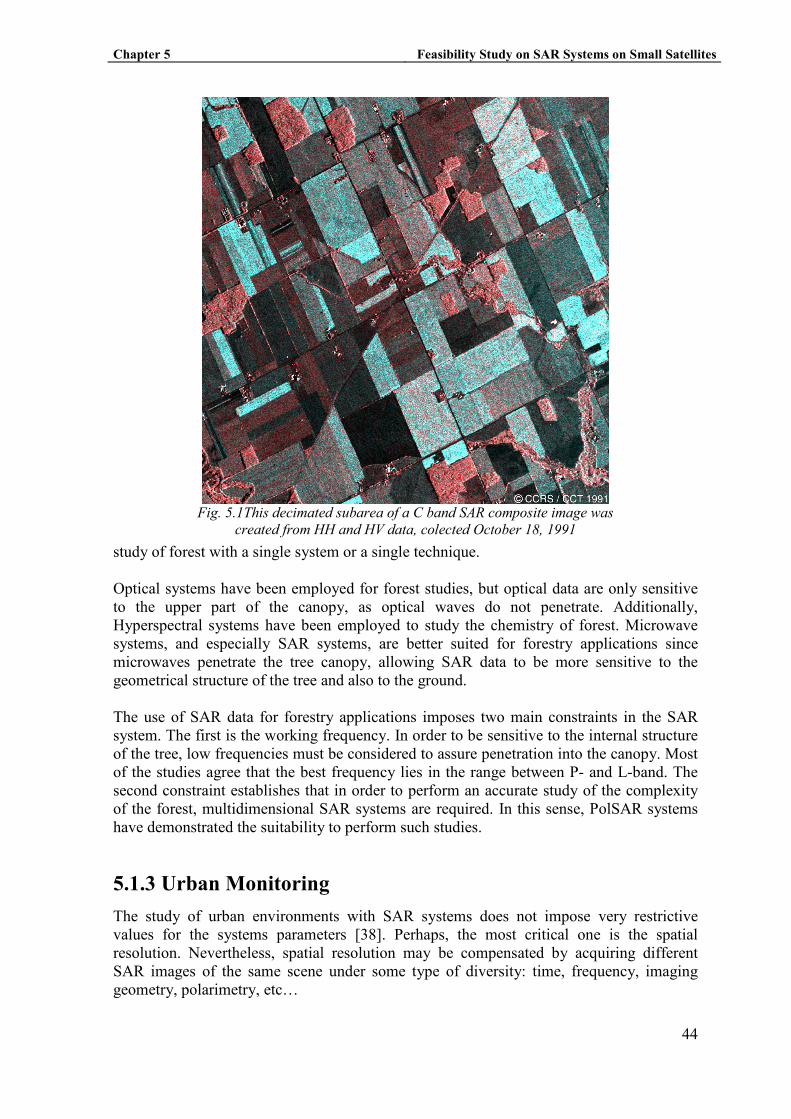
Chapter 5 Feasibility Study on SAR Systems on Small Satellites
44
study of forest with a single system or a single technique.
Optical systems have been employed for forest studies, but optical data are only sensitive
to the upper part of the canopy, as optical waves do not penetrate. Additionally,
Hyperspectral systems have been employed to study the chemistry of forest. Microwave
systems, and especially SAR systems, are better suited for forestry applications since
microwaves penetrate the tree canopy, allowing SAR data to be more sensitive to the
geometrical structure of the tree and also to the ground.
The use of SAR data for forestry applications imposes two main constraints in the SAR
system. The first is the working frequency. In order to be sensitive to the internal structure
of the tree, low frequencies must be considered to assure penetration into the canopy. Most
of the studies agree that the best frequency lies in the range between P- and L-band. The
second constraint establishes that in order to perform an accurate study of the complexity
of the forest, multidimensional SAR systems are required. In this sense, PolSAR systems
have demonstrated the suitability to perform such studies.
5.1.3 Urban Monitoring
The study of urban environments with SAR systems does not impose very restrictive
values for the systems parameters [38]. Perhaps, the most critical one is the spatial
resolution. Nevertheless, spatial resolution may be compensated by acquiring different
SAR images of the same scene under some type of diversity: time, frequency, imaging
geometry, polarimetry, etc…
Fig. 5.1This decimated subarea of a C band SAR composite image was
created from HH and HV data, colected October 18, 1991
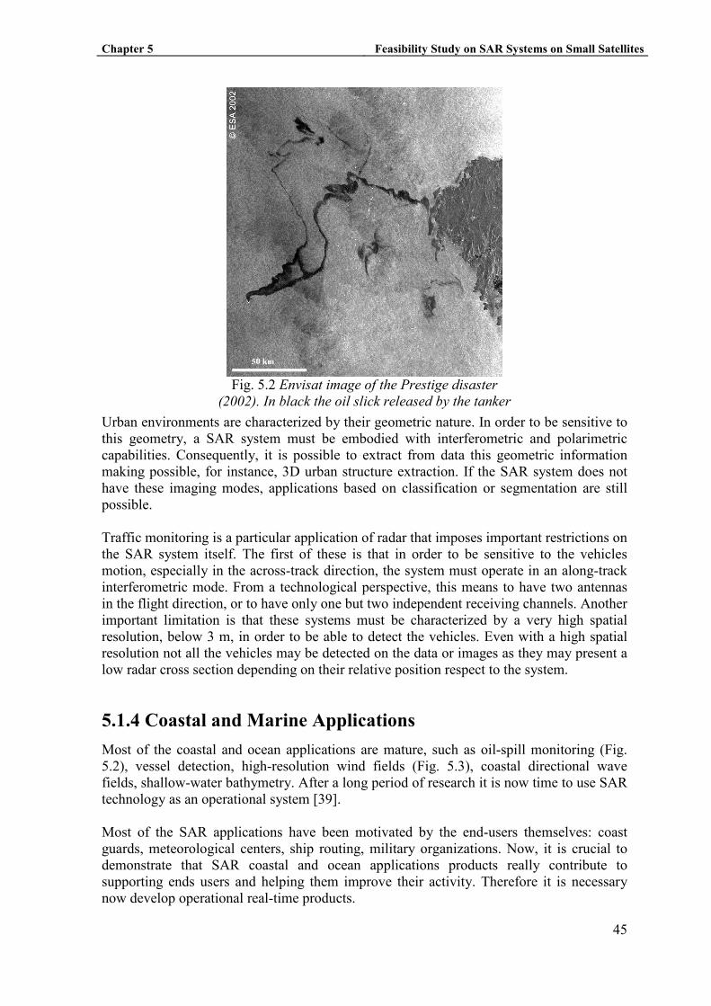
Chapter 5 Feasibility Study on SAR Systems on Small Satellites
45
Urban environments are characterized by their geometric nature. In order to be sensitive to
this geometry, a SAR system must be embodied with interferometric and polarimetric
capabilities. Consequently, it is possible to extract from data this geometric information
making possible, for instance, 3D urban structure extraction. If the SAR system does not
have these imaging modes, applications based on classification or segmentation are still
possible.
Traffic monitoring is a particular application of radar that imposes important restrictions on
the SAR system itself. The first of these is that in order to be sensitive to the vehicles
motion, especially in the across-track direction, the system must operate in an along-track
interferometric mode. From a technological perspective, this means to have two antennas
in the flight direction, or to have only one but two independent receiving channels. Another
important limitation is that these systems must be characterized by a very high spatial
resolution, below 3 m, in order to be able to detect the vehicles. Even with a high spatial
resolution not all the vehicles may be detected on the data or images as they may present a
low radar cross section depending on their relative position respect to the system.
5.1.4 Coastal and Marine Applications
Most of the coastal and ocean applications are mature, such as oil-spill monitoring (Fig.
5.2), vessel detection, high-resolution wind fields (Fig. 5.3), coastal directional wave
fields, shallow-water bathymetry. After a long period of research it is now time to use SAR
technology as an operational system [39].
Most of the SAR applications have been motivated by the end-users themselves: coast
guards, meteorological centers, ship routing, military organizations. Now, it is crucial to
demonstrate that SAR coastal and ocean applications products really contribute to
supporting ends users and helping them improve their activity. Therefore it is necessary
now develop operational real-time products.
Fig. 5.2 Envisat image of the Prestige disaster
(2002). In black the oil slick released by the tanker
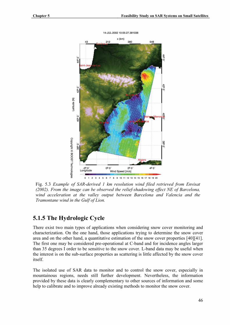
Chapter 5 Feasibility Study on SAR Systems on Small Satellites
46
5.1.5 The Hydrologic Cycle
There exist two main types of applications when considering snow cover monitoring and
characterization. On the one hand, those applications trying to determine the snow cover
area and on the other hand, a quantitative estimation of the snow cover properties [40][41].
The first one may be considered pre-operational at C-band and for incidence angles larger
than 35 degrees I order to be sensitive to the snow cover. L-band data may be useful when
the interest is on the sub-surface properties as scattering is little affected by the snow cover
itself.
The isolated use of SAR data to monitor and to control the snow cover, especially in
mountainous regions, needs still further development. Nevertheless, the information
provided by these data is clearly complementary to other sources of information and some
help to calibrate and to improve already existing methods to monitor the snow cover.
Fig. 5.3 Example of SAR-derived 1 km resolution wind filed retrieved from Envisat
(2002). From the image can be observed the relief-shadowing effect =E of Barcelona,
wind acceleration at the valley output between Barcelona and Valencia and the
Tramontane wind in the Gulf of Lion.
Chapter 5 Feasibility Study on SAR Systems on Small Satellites
47
5.1.6 Cartography
The most important application of SAR technology nowadays is the possibility to obtain
3D topographic maps by means of SAR interferometry (InSAR). This technique is based
on the fact that it is possible to derive topographic information by considering two SAR
acquisitions acquired from slightly different spatial locations. The separation between both
acquisitions is normally referred as baseline. In addition, the two SAR acquisitions may be
obtained at the same time, i.e. single-pass InSAR, or at different times, i.e. repeat-pass
InSAR [42].
The imaging mode of the SAR system, such as strip-map, ScanSAR, and spotlight, play a
special role as they determine the trade-offs between spatial resolution and coverage.
Although high resolution is an obvious requirement, wide swath systems also have their
advantages: given a satellite SAR that is required to image every point of the Earth, a wider
swath width allows for a shorter revisit cycle. This in turn increases scene coherence and is
favourable for repeat-pass InSAR.
Interferometric SARs boarded in space-borne systems is the possibility to perform global
mapping of topography and long-term monitoring of dynamic processes. Satellite data are
at least one order of magnitude cheaper than airborne data. This is particularly true for
inaccessible areas of the Earth. Space-borne remote sensing SAR sensors orbit the Earth at
an altitude of typically 200 km (space shuttle) to 800 km (satellites) at inclinations ranging
from 57º to 108º. Their spatial resolution is usually in the order of 5 m in azimuth and 25
m in ground range allowing for moderate averaging in azimuth for phase noise reduction to
end up with square resolution elements of 25 m2. Nevertheless, the new mission operating
at X-band, as for instance the future TanDEM-X mission, allow to improve the spatial
resolutions up to those obtained with airborne systems The imaged swath is about 50–100
km wide in standard imaging mode and up to 500 km with ScanSAR systems.
5.2 Orbital determination.
Satellites that monitor the global environment, like remote sensing and certain weather
satellites need to scan the entire surface regularly. We have to understand satellites as a
global tool and, therefore, design accordingly the most appropriate mission.
The mission’s orbital design should be performed adjusting the following 6 parameters:
1. The inclination of the orbital plane.
2. The longitude of the ascending nodal line.
3. The perigee angle obtained from the ascending node.
4. The semi-major axis of the ellipse.
5. The eccentricity of the orbit.
6. The pass time at the perigee (reference initial time).
The most usual orbit for earth-mapping, earth observation, and reconnaissance satellites, as
well as for some weather satellites, is a polar, or near-polar, orbit. The ground track of a
polar orbiting satellite is displaced to the west after each orbital period, due to the rotation
of the Earth. This displacement of longitude is a function of the orbital period (often less
than 2 hours for low altitude orbits). Depending on the ground swath of the satellite, it is

Chapter 5 Feasibility Study on SAR Systems on Small Satellites
48
possible to adjust the period (by varying the altitude), and thus the longitudinal
displacement, in such a way as to ensure the observation of any point on the Earth within a
certain time period.
It is common for polar orbiting satellites to choose a sun-synchronous orbit, each
successive orbital pass occurs at the same local time of day. They can be particularly
important for applications, where the most important thing to see may well be changes over
time, which you do not want to see aliased onto changes in local time. This is an important
factor for monitoring changes between images or for mosaicking adjacent images together,
as they do not have to be corrected for different illumination conditions. To keep the same
local time on a given pass, it is desirable for the orbit to be as short as possible, which is to
say as low as possible.
In order to earth/sun-synchronize the satellite, the orbit altitude has been increased around
11 km from de 500 km assumed in Fig. 2.3. The inclination of the orbital plane must be
97’41º. An example of the track described for the satellite while crossing Catalonia is
shown inFig. 5.4.
The disadvantage to polar orbit is that no one spot on the Earth's surface can be sensed
continuously. It is not suitable for applications in which a little (hours or one day) revisit
time is needed. To achieve a polar orbit requires more energy, thus more propellant, than
does an orbit of low inclination. It cannot take advantage of the “free ride” provided by the
Earth’s rotation, and thus the launch vehicle must provide all of the energy for attaining
orbital speed.
From the list of applications described in chapter 5.1 we can implement the ones that do
not required little revisit time. Enhancing terrain features for cartography, detecting small
surface movements, improving the agriculture procedures by giving information of influent
parameters for the harvest…
The orbital parameters described have been summarized in Table 5.1
Nominal orbit height at the equator 511,449 km
Orbits per day 15 + 1/5
Repeat cycle 5 days
Inclination 97,41 º
Table 5.1 Orbital Parameters
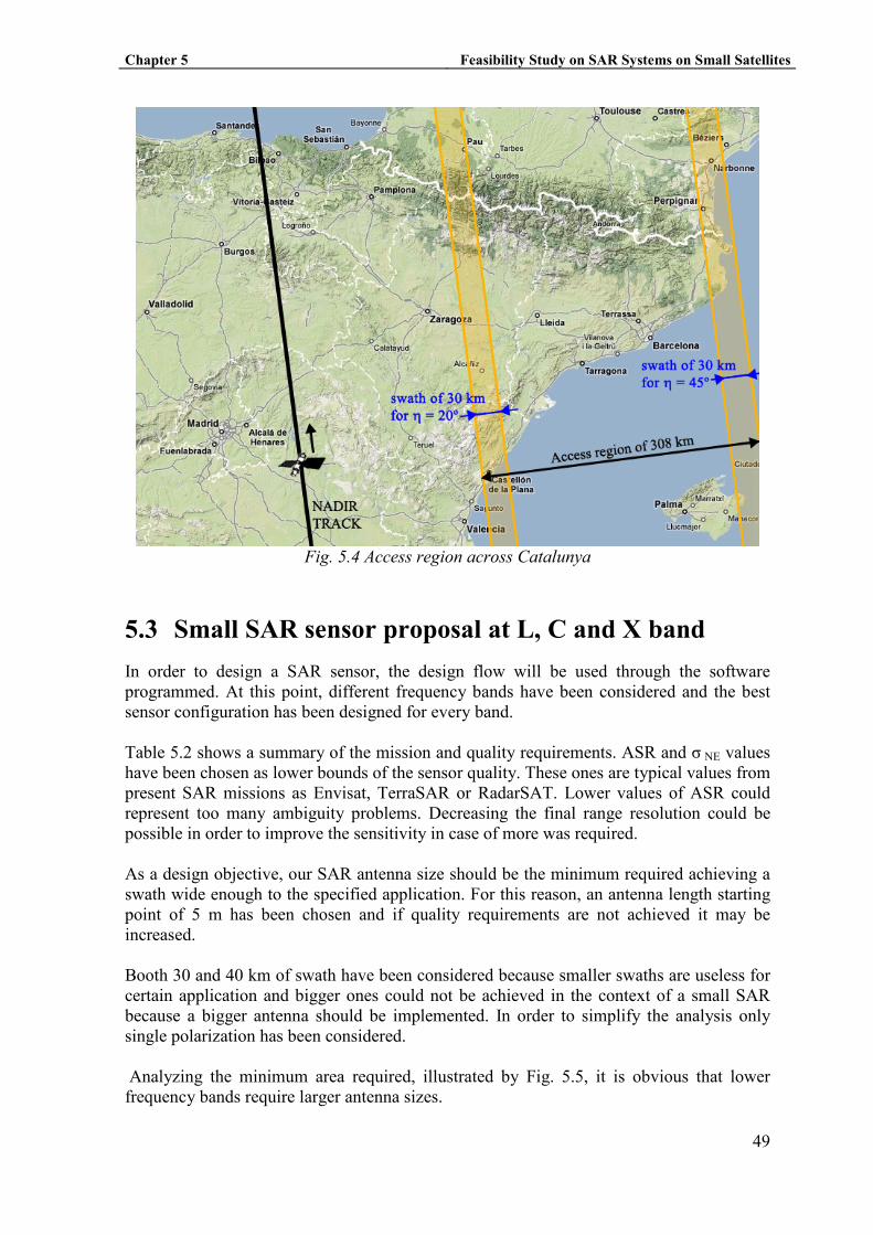
Chapter 5 Feasibility Study on SAR Systems on Small Satellites
49
5.3 Small SAR sensor proposal at L, C and X band
In order to design a SAR sensor, the design flow will be used through the software
programmed. At this point, different frequency bands have been considered and the best
sensor configuration has been designed for every band.
Table 5.2 shows a summary of the mission and quality requirements. ASR and σ NE values
have been chosen as lower bounds of the sensor quality. These ones are typical values from
present SAR missions as Envisat, TerraSAR or RadarSAT. Lower values of ASR could
represent too many ambiguity problems. Decreasing the final range resolution could be
possible in order to improve the sensitivity in case of more was required.
As a design objective, our SAR antenna size should be the minimum required achieving a
swath wide enough to the specified application. For this reason, an antenna length starting
point of 5 m has been chosen and if quality requirements are not achieved it may be
increased.
Booth 30 and 40 km of swath have been considered because smaller swaths are useless for
certain application and bigger ones could not be achieved in the context of a small SAR
because a bigger antenna should be implemented. In order to simplify the analysis only
single polarization has been considered.
Analyzing the minimum area required, illustrated by Fig. 5.5, it is obvious that lower
frequency bands require larger antenna sizes.
Fig. 5.4 Access region across Catalunya
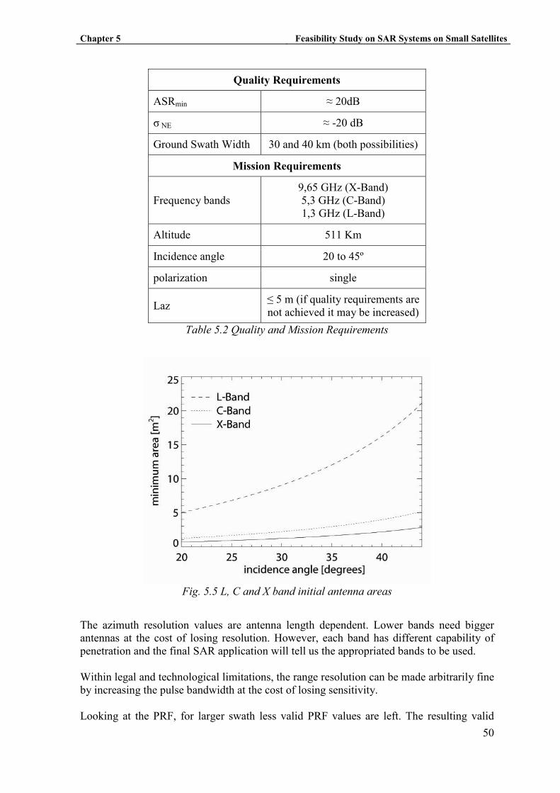
Chapter 5 Feasibility Study on SAR Systems on Small Satellites
50
The azimuth resolution values are antenna length dependent. Lower bands need bigger
antennas at the cost of losing resolution. However, each band has different capability of
penetration and the final SAR application will tell us the appropriated bands to be used.
Within legal and technological limitations, the range resolution can be made arbitrarily fine
by increasing the pulse bandwidth at the cost of losing sensitivity.
Looking at the PRF, for larger swath less valid PRF values are left. The resulting valid
Fig. 5.5 L, C and X band initial antenna areas
Quality Requirements
ASRmin ≈ 20dB
σ NE ≈ -20 dB
Ground Swath Width 30 and 40 km (both possibilities)
Mission Requirements
Frequency bands
9,65 GHz (X-Band)
5,3 GHz (C-Band)
1,3 GHz (L-Band)
Altitude 511 Km
Incidence angle 20 to 45º
polarization single
Laz ≤ 5 m (if quality requirements are
not achieved it may be increased)
Table 5.2 Quality and Mission Requirements
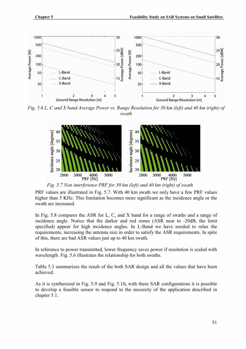
Chapter 5 Feasibility Study on SAR Systems on Small Satellites
51
PRF values are illustrated in Fig. 5.7. With 40 km swath we only have a few PRF values
higher than 5 KHz. This limitation becomes more significant as the incidence angle or the
swath are increased.
In Fig. 5.8 compares the ASR for L, C, and X band for a range of swaths and a range of
incidence angle. Notice that the darker and red zones (ASR near to -20dB, the limit
specified) appear for high incidence angles. In L-Band we have needed to relax the
requirements, increasing the antenna size in order to satisfy the ASR requirements. In spite
of this, there are bad ASR values just up to 40 km swath.
In reference to power transmitted, lower frequency saves power if resolution is scaled with
wavelength. Fig. 5.6 illustrates the relationship for both swaths.
Table 5.3 summarizes the result of the both SAR design and all the values that have been
achieved.
As it is synthesized in Fig. 5.9 and Fig. 5.10, with these SAR configurations it is possible
to develop a feasible sensor to respond to the necessity of the application described in
chapter 5.1.
Fig. 5.6 L, C and X band Average Power vs. Range Resolution for 30 km (left) and 40 km (right) of
swath
Fig. 5.7 =on interference PRF for 30 km (left) and 40 km (right) of swath
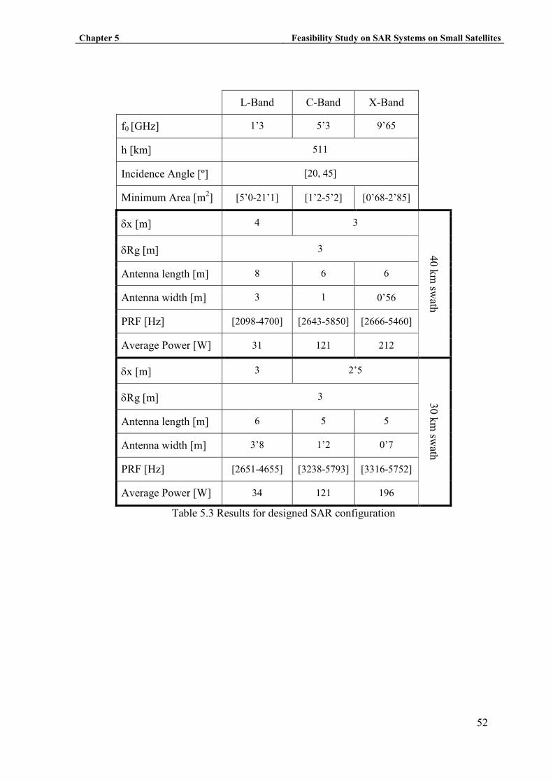
Chapter 5 Feasibility Study on SAR Systems on Small Satellites
52
L-Band C-Band X-Band
f0 [GHz] 1’3 5’3 9’65
h [km] 511
Incidence Angle [º] [20, 45]
Minimum Area [m2] [5’0-21’1] [1’2-5’2] [0’68-2’85]
δx [m] 4 3
40 k
m sw
ath
δRg [m] 3
Antenna length [m] 8 6 6
Antenna width [m] 3 1 0’56
PRF [Hz] [2098-4700] [2643-5850] [2666-5460]
Average Power [W] 31 121 212
δx [m] 3 2’5
30 k
m sw
ath
δRg [m] 3
Antenna length [m] 6 5 5
Antenna width [m] 3’8 1’2 0’7
PRF [Hz] [2651-4655] [3238-5793] [3316-5752]
Average Power [W] 34 121 196
Table 5.3 Results for designed SAR configuration
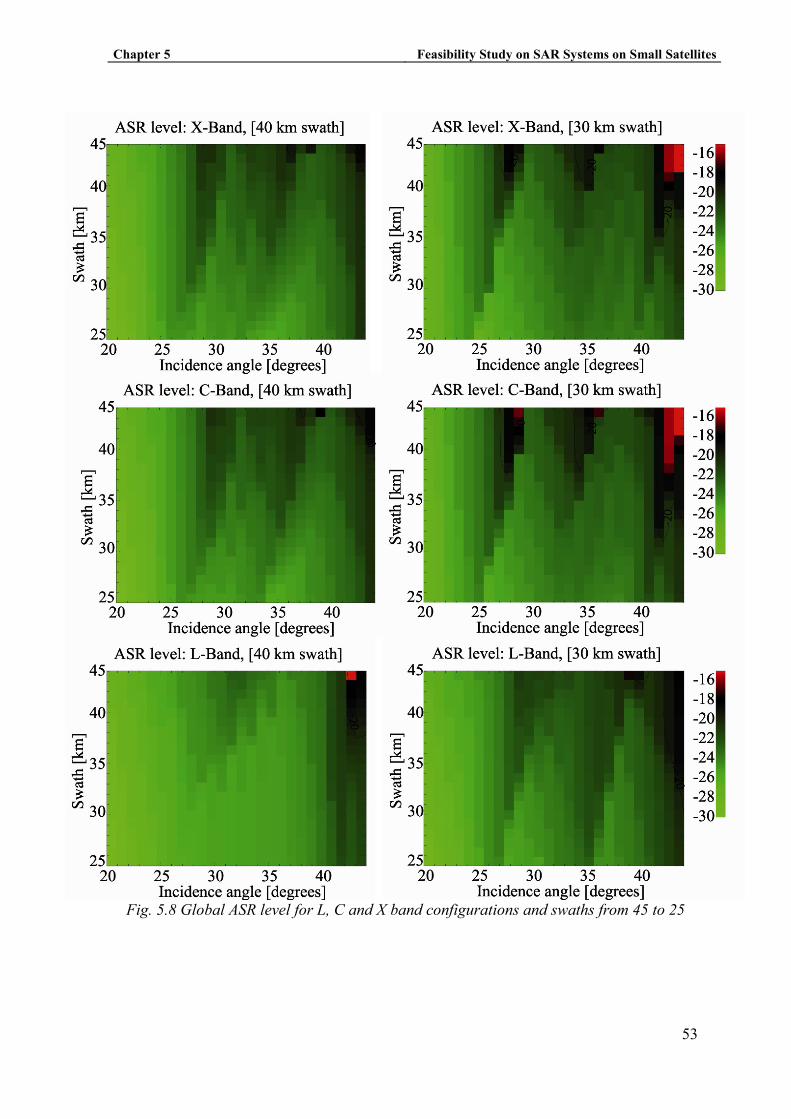
Chapter 5 Feasibility Study on SAR Systems on Small Satellites
53
Fig. 5.8 Global ASR level for L, C and X band configurations and swaths from 45 to 25

Chapter 5 Feasibility Study on SAR Systems on Small Satellites
54
5.4 Data storage and down link.
A major constraint in the design of most current space-borne SAR systems is the available
downlink data rate. For SAR systems, the swath width is either data rate limited or the
system dynamic range has been degraded by reduced the number of bits per sample.
Considering the mission designed before the downlink capacity can be calculated with this
Fig. 5.9 Capability of the three sensors designed in front of operational SAR
applications
Fig. 5.10 Capability of the three sensors designed in front of experimental SAR
applications

Chapter 5 Feasibility Study on SAR Systems on Small Satellites
55
considerations:
• Quantization [ ] 1.8
56
b
S=R dB=
−= = bits/sample
• Bandwidth ,2 sin
R
g
cB
Rδ η= incidence angle dependent
• PRF valid values (from 2666 to 5460) that optimize the .ASR.
• Swath width Sw = 40km
• Pulse time τp=30 µs
The required minimum slant range swath is approximately
Slantswath swath sin( ) 28Kmη≅ ⋅ =
wich corresponds to a observation time of
w slant p=2swath c + = 123 sτ τ µ
Assuming an oversampling factor gor = 1.2, the sampling frequency is fs = 84 Msamples/s.
The number of samples per range line is therefore
r s wN = f . = 10,332 samplesτ
and the instantaneous data rate is
i b sr = n .f = 420 Mbps
Assuming the ADC output is buffered to achieve time expansion over the entire inter-pulse
period, the average (sustained) real-time downlink data rate is
DL w ir = .r .PRF τ
and using the minimum and the maximum PRF values:
rDLmax= 282,06Mbps
rDLmin= 137,72 Mbps
Typically a downlink rate of these magnitudes cannot be achieved, since it would require a
large downlink transmitter and antenna subsystem that cannot be accommodated within the
platform resources, given the large mass and power requirements of the SAR. The
alternative is to reduce the system performance by modifying either the system design or
the data collection procedure. Among the available options are:
1- Increase the azimuth length (Laz) of the SAR antenna and reduce the PRF and/or the
azimuth oversampling factor (goa) at the cost of increased mass and degraded
azimuth resolution;
Chapter 5 Feasibility Study on SAR Systems on Small Satellites
56
2- Reduce the system Bandwidth (BR) and/or the range oversampling factor (gor) at the
cost of range resolution;
3- Reduce the Swath or change the imaging geometry to a steeper incidence angle (η)
at the cost of ground coverage and increased geometric distorsion from
foreshortening and layover effects
4- Reduce the quantization to fewer bits per sample (nb) at the cost of increased
distorsion noise and therefore a degraded impulse response function and
radiometric calibration accuracy.
If an onboard processor were available to generate the image data in real time, the
resolution degradation could be performed by multilook averaging, thus reducing the
speckle noise in the process.
Chapter 6 Feasibility Study on SAR Systems on Small Satellites
57
6 SUMMARY, CO�CLUSIO�S A�D FUTURE
LI�ES
6.1 Summary
The global context analyzed has showed us that nowadays, there is a trend toward
designing satellite SAR missions more compact and in lower orbits. At this point, some
questions appear in engineers minds: How small can we make a SAR system?
As the SAR system was designed to be boarded on a compact satellite, the antenna must be
as small as possible. However, the price of reducing the antenna is:
• Reduced Swath (smaller images and revisit time increased)
• Reduced Ambiguity rejection
• More power required (without varying the altitude)
Because of this trade-off, the antenna size is not technological limited. However, a smaller
antenna than the specified in Table 5.3 cannot be designed with the restrictions specified in
Table 5.2.
Relaxing the ASR restriction and the swath width can help to design a smaller antenna but
also can make the system data useless for most applications.
Bigger antennas are needed in lower frequency bands to satisfy the same restrictions. For
this reason new missions planned are tending to board X-band systems.
For applications such as agricultural or forestry, L-band systems could be more appealing
than C or X-band ones because of lower power is required. However, the penetration depth
required for the application will determinate which should be the system frequency.
In terms of resolution, it seems that resolutions around a few meters are the maximum
allowable for the system. For application with more precision like traffic monitoring, it
could be necessary to reduce the satellite altitude in order to reduce power required and
antenna size.
6.2 Conclusions
Compact platform are a good opportunity to design systems with good trade-offs between
performance and costs than other big satellites missions.
According with the results of the designed SAR mission proposal, a SAR on a compact
platform is feasible, with a certain degree. In order to establish a reference mission, a
smaller satellite than TerraSAR-X could have problems to achieve the minimum
Chapter 6 Feasibility Study on SAR Systems on Small Satellites
58
requirements for actual operational applications.
In the PCOT context, the design of a SAR system mission intended for cartography
applications and much cheaper than TerraSAR-X mission it seems it would be not feasible
with the current technology.
Analyzing the global context, Low Earth Orbit satellites are a global tool and it is useless
to develop a SAR system only to use it in a concrete region. For this reason most of the
missions are planned from partnerships in which research centers as the NASA (National
Aeronautics and Space Administration) or the ESA (European Space Agency) are
involved.
The solution to the PCOT SAR necessity could be other cheaper platforms as planes or
zeppelins in order to design local missions.
6.3 Future lines
The study done could be extended by introducing new SAR concepts such as high
resolution wide swath modes, new SAR antennas concepts working in other bands not
mentioned, etc
In the mission design, satellite mass payload has not been determined and it could be
interesting to study the antenna limit mass to establish its maximum weight.
Moreover, the satellite ground segment need to be designed: downlink antenna, control
centre, mission control systems, planning and scheduling, simulator, payload data
processing and archive.
The satellite altitude has been assumed from the recent missions so a extended study
should include other types of compact missions such as unnamed and stratospheric
platforms. They could be a good alternative to satellites for certain applications, or even a
good complement.
Constellation missions are gaining special prominence in near future planned missions.
• Tandem-X (TerraSAR-X add-on for Digital Elevation Measurements) is a second,
very similar spacecraft that will orbit in a close formation flight with TerraSAR-X,
scheduled to be launched in 2009 [43].
• The Italian COSMO-SkyMed mission is a 4-spacecraft constellation, each equipped
with X-band SAR. The first satellite was launched in June 2007, the second in
December 2007, the third in October 2008 with the fourth satellite scheduled for
launch in 2010.
A second version of the software could be programmed reducing some time process
functions and introducing new features like orbit or downlink design

Feasibility Study on SAR Systems on Small Satellites
59

References Feasibility Study on SAR Systems on Small Satellites
60
REFERE�CES
[1] SEASAT Home Page http://southport.jpl.nasa.gov/scienceapps/seasat.html
[2] SIR-A Home Page http://southport.jpl.nasa.gov/scienceapps/sira.html
[3] SIR-B Home Page http://southport.jpl.nasa.gov/scienceapps/sirb.html
[4] Magellan Home Page http://www2.jpl.nasa.gov/magellan/fact.html
[5] European Space Agency Home Page http://earth.esa.int/ers/satconc/
[6] http://www.esa.int/esaEO/SEMGWH2VQUD_index_0_m.html
[7] http://envisat.esa.int/object/index.cfm?fobjectid=3760
[8] SIR-C Home Page http://southport.jpl.nasa.gov/sir-c/
[9] European Space Agency Home Page http://earth.esa.int/ers/
[10] Canadian Space Agency Home Page
http://www.asc-csa.gc.ca/eng/satellites/radarsat1/default.asp
[11] Shuttle Radar Topography Mission Home Page http://www2.jpl.nasa.gov/srtm/
[12] Envisat Home Page http://envisat.esa.int/
[13] Japan Aerospace Exploration Agency Home Page
http://www.jaxa.jp/projects/sat/alos/index_e.html
[14] Jörg Herrmann, Alejandra González Bottero, “TerraSAR-X Mission: The New
Generation in High Resolution Satellites”, Anais XIII Simpósio Brasileiro de
Sensoriamento Remoto, Florianópolis, Brasil, 21-26 abril 2007, INPE, Pages: 7063-
7070.
[15] Rolf Werninghaus, Wolfgang Balzer, Stefan Buckreuss, Josef Mittermayer, Peter
Mühlbauer , “TerraSAR-X Mission”,
http://www.dlr.de/tsx/documentation/EUSAR-TX-Mission.pdf
[16] Radarsat Home Page http://www.radarsat2.info/
[17] OHB-System AG, Universitätsallee 27–29, The SAR-LUPE Programm-An
Industrial View -Security and Defence Aspects of Space:The Challenges for
EUAthens, Greece, May 8-9, 2003,
http://ec.europa.eu/comm/space/doc_pdf/merkle.pdf
References Feasibility Study on SAR Systems on Small Satellites
61
[18] OHB-System AG, Universitätsallee 27–29, “SAR-Lupe, The innovative program
for satellite-based radar reconnaissance” http://www.ohb-system.de/pdf/sar-lupe-
broschure.pdf
[19] SAR-Lupe Constellation
http://directory.eoportal.org/pres_SARLupeConstellation.html
[20] JianBing 5 (YaoGan WeiXing 1/3) Synthetic Aperture Radar Satellite
http://www.sinodefence.com/strategic/spacecraft/jianbing5.asp
[21] Tuyuan Technologies "Surveyor" Satellite Constellation
http://www.spaceref.com/news/viewpr.html?pid=14919
[22] China Plans Commercial SAR EO Constellation”
http://news.eoportal.org/eomissions/040907_surveyo.html
[23] Alcatel Alenia Space Radar System For The Korean EO Sat Kompsat-5,
http://www.spacemart.com/reports/Alcatel_Alenia_Space_Radar_System_For_The
_Korean_EO_Sat_Kompsat_5.html
[24] Ian Hønstvet , Ian Encke , David Hall , Yvonne Munro “ASTROSAR-LITE – A
RADAR SYSTEM FOR THE TROPICS” Anais XIII Simpósio Brasileiro de
Sensoriamento Remoto, Florianópolis, Brasil, 21-26 abril 2007, INPE, p. 4907-
4913.
[25] Attema, E., 2005. Mission Requirements ,Document for the European Radar
Observatory Sentinel-1, ESA, ES-RS-ESA-SY-0007, Noordwijk, The Netherlands,
http://esamultimedia.esa.int/docs/GMES/GMES_SENT1_MRD_1-
4_approved_version.pdf
[26] Reinhard Schröder, Jürgen Puls, Irena Hajnsek, Fritz Jochim, Thomas Neff, Janio
Kono,Waldir Renato Paradella, Mario Marcos Quintino da Silva, Dalton de
Morisson Valeriano, Maycira Pereira Farias Costa, “MAPSAR: a small L-band
SAR mission for land observation”, Acta Astronáutica 56 (2005), Pages: 35 – 43
[27] Vincent, N.; Gaillard, D.; Banos, T.; “Small satellite system for civilian radar
imagery application”, Geoscience and Remote Sensing Symposium Proceedings,
1998. IGARSS '98. 1998 IEEE International, Volume 1, 6-10 July 1998 Pages:
274 - 276 vol.1
[28] Aguttes, J.P., “High resolution (metric) SAR microsatellite, based on the CNES
MYRIADE bus”, Geoscience and Remote Sensing Symposium, 2001. IGARSS '01.
IEEE 2001 International, Volume 1, 9-13 July 2001 Pages:224 - 226 vol.1
[29] Albert Aguasca Solé, Antoni Broquetas Ibars, Adriano Camps Carmona, Xavier
Fàbregas Cànovas, Albert García Mondéjar, Paco López Dekker, Carlos López
Martínez, Jordi Mallorquí Franquet, SARMISP: “ SAR Mission on Small
Platforms” December 2008
[30] Ulaby, F.T., R.K. Moore and A.K. Fung (1982). Microwave Remote Sensing, Vol.
References Feasibility Study on SAR Systems on Small Satellites
62
2, Addison-Wesley, Reading, MA.
[31] Cutrona , L.J. (1970) “Synthetic Aperture Radar”, Chapter 23 in Radar Handbook
(Skolnik, M.I.,ed.) McGraw-Hill, New York
[32] John C. Curlander and Robert N. McDonough (1991)“Synthetic Aperture Radar –
systems and Signal Processing” Wiley series in remote sensing.
[33] http://www.mityc.es/Telecomunicaciones/Secciones/Espectro/cnaf/
[34] Boerner W.-M., Mott H., Lunenburg E., Livingstone C., Brisco B., Brown R. J.,
Patterson J. S. Polarimetry in Remote Sensing: Basic and Applied Concepts,
chapter 5: in Manual of Remote Sensing, Volume 2: Principles and Applications of
Imaging Radar. Wiley, 3rd edition, 1998.
[35] Sauer, S.; Ferro-Famil, L.; Reigber, A.; Pottier, E., "Multibaseline POL-InSAR analysis of
urban scenes for 3D modeling and physical feature retrieval at L-band," Geoscience and
Remote Sensing Symposium, 2007. IGARSS 2007. IEEE International , vol., no., pp.1098-
1101, 23-28 July 2007
[36] Bayman, R.W. and P.A. McInnes (1975). “Aperture Size and Ambiguity
Constraints for Synthetic Aperture Radar,” IEEE 1975 Inter. Radar Conf., pp.49-
504
[37] Kühbauch, W.; Hawlitschka, S., “Remote Sensing - A Future Technology in
Precision Farming,” Pol-InSAR 2003, Frascati, Italy, January 2003
[38] C. Lin and R. Päivinen, “Forestry user requirement assessment – the SAR for
Agriculture and Forestry in Europe (SAFE) project experiences and results,”
Retrieval of Bio- and Geo-Physical Parameters from SAR Data for Land
Applications Workshop ESTEC, 21-23 October 1998
[39] Vincent Kerboal, Fabrice Collard “SAR-Derived Coastal and Marine Applications:
From Research to Operational Products”, IEEE Journal of Oceananic Engineering,
Vol. 30, Nº 3, July 2005
[40] Lee, J., Schuler, T., Krogager, E. & Kasilingam, W. “On the estimation of radar
polarization orientation shifts induced by terrain slopes”, Geoscience and Remote
Sensing, IEEE Transactions on, vol. 40, pp 30-41 , 2002.
[41] L. Tsang, J.A. Kong and R.T. Shin. “Theory of Microwave Remote Sensing”,
Wiley Interscience Publication, New York, 1985.
[42] Zebker H A and Goldstein R M 1986 Topographic mapping from interferometric
synthetic aperture radar observations J. Geophys. Res. 91 4993–9
[43] Tandem-X http://www.infoterra.de/terrasar-x/tandem-x-mission.html
[44] COSMO-Skymed
http://www.deagel.com/C3ISTAR-Satellites/COSMO-SkyMed_a000256001.aspx

Feasibility Study on SAR Systems on Small Satellites
63
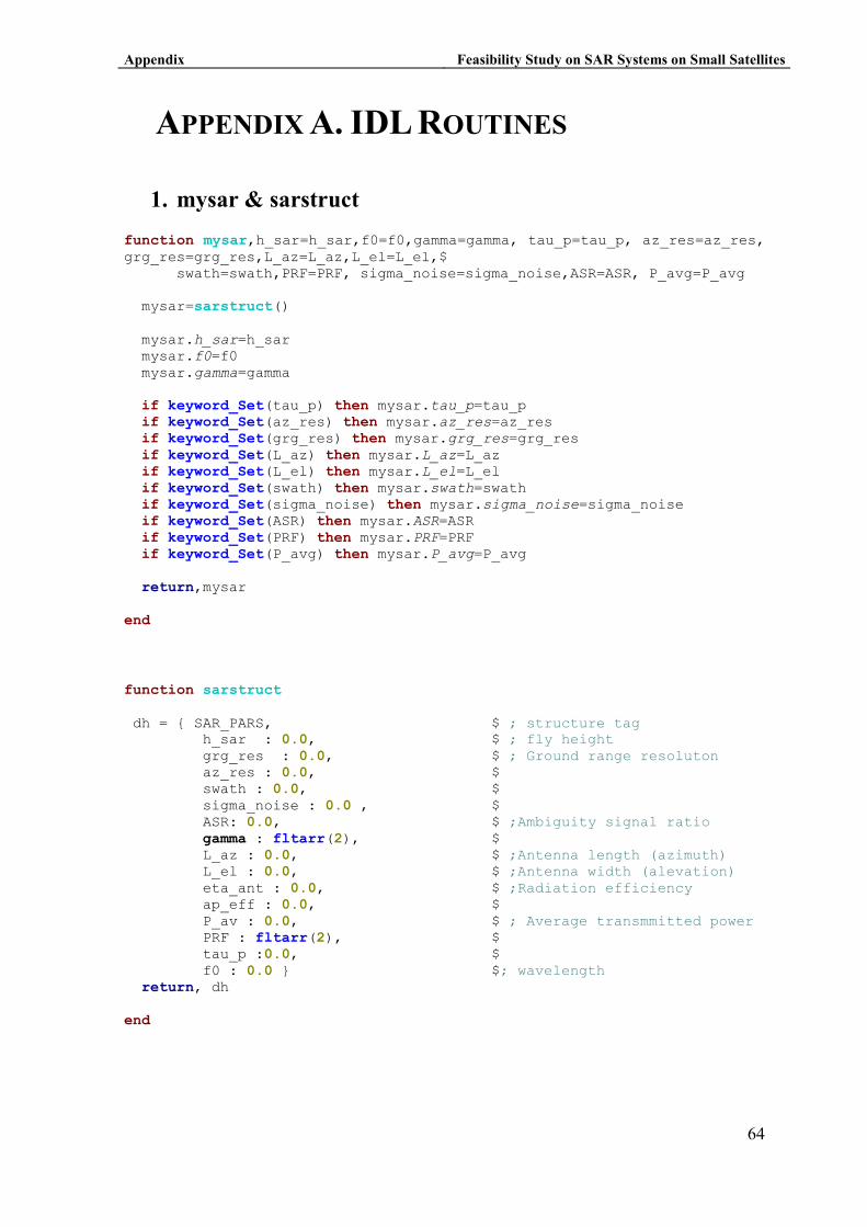
Appendix Feasibility Study on SAR Systems on Small Satellites
64
APPE�DIX A. IDL ROUTI�ES
1. mysar & sarstruct function mysar,h_sar=h_sar,f0=f0,gamma=gamma, tau_p=tau_p, az_res=az_res, grg_res=grg_res,L_az=L_az,L_el=L_el,$ swath=swath,PRF=PRF, sigma_noise=sigma_noise,ASR=ASR, P_avg=P_avg mysar=sarstruct() mysar.h_sar=h_sar mysar.f0=f0 mysar.gamma=gamma if keyword_Set(tau_p) then mysar.tau_p=tau_p if keyword_Set(az_res) then mysar.az_res=az_res if keyword_Set(grg_res) then mysar.grg_res=grg_res if keyword_Set(L_az) then mysar.L_az=L_az if keyword_Set(L_el) then mysar.L_el=L_el if keyword_Set(swath) then mysar.swath=swath if keyword_Set(sigma_noise) then mysar.sigma_noise=sigma_noise if keyword_Set(ASR) then mysar.ASR=ASR if keyword_Set(PRF) then mysar.PRF=PRF if keyword_Set(P_avg) then mysar.P_avg=P_avg return,mysar end
function sarstruct dh = { SAR_PARS, $ ; structure tag h_sar : 0.0, $ ; fly height grg_res : 0.0, $ ; Ground range resoluton az_res : 0.0, $ swath : 0.0, $ sigma_noise : 0.0 , $ ASR: 0.0, $ ;Ambiguity signal ratio gamma : fltarr(2), $ L_az : 0.0, $ ;Antenna length (azimuth) L_el : 0.0, $ ;Antenna width (alevation) eta_ant : 0.0, $ ;Radiation efficiency ap_eff : 0.0, $ P_av : 0.0, $ ; Average transmmitted power PRF : fltarr(2), $ tau_p :0.0, $ f0 : 0.0 } $; wavelength return, dh end
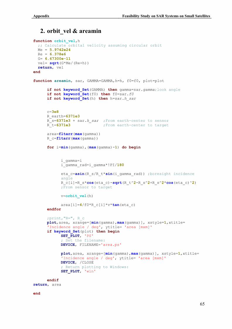
Appendix Feasibility Study on SAR Systems on Small Satellites
65
2. orbit_vel & areamin function orbit_vel,h ;; Calculate orbital velicity assuming circular orbit Me = 5.9742e24 Re = 6.378e6 G= 6.67300e-11 vel= sqrt(G*Me/(Re+h)) return, vel end function areamin, sar, GAMMA=GAMMA,h=h, f0=f0, plot=plot
if not keyword_Set(GAMMA) then gamma=sar.gamma;look angle if not keyword_Set(f0) then f0=sar.f0 if not keyword_Set(h) then h=sar.h_sar
c=3e8 R_earth=6371e3 R_s=6371e3 + sar.h_sar ;From earth-center to sensor R_t=6371e3 ;From earth-center to target
area=fltarr(max(gamma)) R_c=fltarr(max(gamma))
for i=min(gamma),(max(gamma)-1) do begin
i_gamma=i i_gamma_rad=i_gamma*!PI/180
eta_c=asin(R_s/R_t*sin(i_gamma_rad)) ;boresight incidence angle R_c[i]=R_s*cos(eta_c)-sqrt(R_t^2-R_s^2+R_s^2*cos(eta_c)^2) ;From sensor to target
v=orbit_vel(h) area[i]=4/f0*R_c[i]*v*tan(eta_c)
endfor ;print,"R=", R_c
plot,area, xrange=[min(gamma),max(gamma)], xstyle=1,xtitle= 'Incidence angle / deg', ytitle= 'area [mxm]'
if keyword_Set(plot) then begin SET_PLOT, 'PS' ; Set the filename: DEVICE, FILENAME='area.ps'
plot,area, xrange=[min(gamma),max(gamma)], xstyle=1,xtitle= 'Incidence angle / deg', ytitle= 'area [mxm]'
DEVICE, /CLOSE ; Return plotting to Windows: SET_PLOT, 'win' endif return, area end
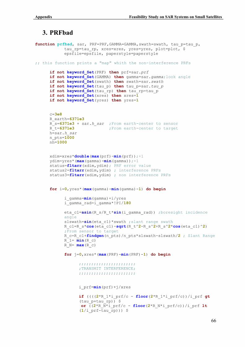
Appendix Feasibility Study on SAR Systems on Small Satellites
66
3. PRFbad function prfbad, sar, PRF=PRF,GAMMA=GAMMA,swath=swath, tau_p=tau_p,
tau_rp=tau_rp, xres=xres, yres=yres, plot=plot, $ epsfile=epsfile, paperstyle=paperstyle
;; this function prints a "map" whith the non-interference PRFs
if not keyword_Set(PRF) then prf=sar.prf if not keyword_Set(GAMMA) then gamma=sar.gamma;look angle if not keyword_Set(swath) then swath=sar.swath if not keyword_Set(tau_p) then tau_p=sar.tau_p if not keyword_Set(tau_rp) then tau_rp=tau_p if not keyword_Set(xres) then xres=1 if not keyword_Set(yres) then yres=1
c=3e8 R_earth=6371e3 R_s=6371e3 + sar.h_sar ;From earth-center to sensor R_t=6371e3 ;From earth-center to target h=sar.h_sar n_pts=1000 nh=1000
xdim=xres*double(max(prf)-min(prf));+1 ydim=yres*(max(gamma)-min(gamma));+1 status=fltarr(xdim,ydim); PRF error value status2=fltarr(xdim,ydim) ; interference PRFs status3=fltarr(xdim,ydim) ; non interference PRFs
for i=0,yres*(max(gamma)-min(gamma)-1) do begin
i_gamma=min(gamma)+i/yres i_gamma_rad=i_gamma*!PI/180
eta_c1=asin(R_s/R_t*sin(i_gamma_rad)) ;boresight incidence angle slswath=sin(eta_c1)*swath ;slant range swath R_c1=R_s*cos(eta_c1)-sqrt(R_t^2-R_s^2+R_s^2*cos(eta_c1)^2) ;From sensor to target R_c=R_c1+findgen(n_pts)/n_pts*slswath-slswath/2 ; Slant Range R_1= min(R_c) R_N= max(R_c)
for j=0,xres*(max(PRF)-min(PRF)-1) do begin
;;;;;;;;;;;;;;;;;;;;;;; ;TRANSMIT INTERFERENCE; ;;;;;;;;;;;;;;;;;;;;;;;
i_prf=min(prf)+j/xres if ((((2*R_1*i_prf/c - floor(2*R_1*i_prf/c))/i_prf gt (tau_p+tau_rp)) $ or ((2*R_N*i_prf/c - floor(2*R_N*i_prf/c))/i_prf lt (1/i_prf-tau_rp))) $
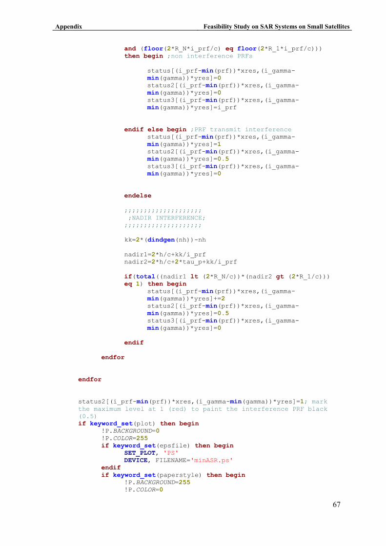
Appendix Feasibility Study on SAR Systems on Small Satellites
67
and (floor(2*R_N*i_prf/c) eq floor(2*R_1*i_prf/c))) then begin ;non interference PRFs
status[(i_prf-min(prf))*xres,(i_gamma-min(gamma))*yres]=0 status2[(i_prf-min(prf))*xres,(i_gamma-min(gamma))*yres]=0 status3[(i_prf-min(prf))*xres,(i_gamma-min(gamma))*yres]=i_prf
endif else begin ;PRF transmit interference status[(i_prf-min(prf))*xres,(i_gamma-min(gamma))*yres]=1 status2[(i_prf-min(prf))*xres,(i_gamma-min(gamma))*yres]=0.5 status3[(i_prf-min(prf))*xres,(i_gamma-min(gamma))*yres]=0
endelse
;;;;;;;;;;;;;;;;;;;; ;NADIR INTERFERENCE; ;;;;;;;;;;;;;;;;;;;;
kk=2*(dindgen(nh))-nh
nadir1=2*h/c+kk/i_prf nadir2=2*h/c+2*tau_p+kk/i_prf
if(total((nadir1 lt (2*R_N/c))*(nadir2 gt (2*R_1/c))) eq 1) then begin
status[(i_prf-min(prf))*xres,(i_gamma-min(gamma))*yres]+=2 status2[(i_prf-min(prf))*xres,(i_gamma-min(gamma))*yres]=0.5 status3[(i_prf-min(prf))*xres,(i_gamma-min(gamma))*yres]=0
endif
endfor
endfor
status2[(i_prf-min(prf))*xres,(i_gamma-min(gamma))*yres]=1; mark the maximum level at 1 (red) to paint the interference PRF black (0.5) if keyword_set(plot) then begin
!P.BACKGROUND=0 !P.COLOR=255 if keyword_set(epsfile) then begin SET_PLOT, 'PS' DEVICE, FILENAME='minASR.ps' endif if keyword_set(paperstyle) then begin !P.BACKGROUND=255 !P.COLOR=0

Appendix Feasibility Study on SAR Systems on Small Satellites
68
endif !P.MULTI = 0 image,status2,xmin=min(PRF),xmax=max(PRF),ymin=min(GAMMA),ymax=max( GAMMA),NOCOLORBAR=1,XTITOL='PRF [Hz]',YTITOL='Incidence angle [degrees]',PAPERSTYLE=1, charsize=1.5 ;, pngfile='prfbad2.png' if keyword_set(epsfile) then begin DEVICE, /CLOSE SET_PLOT, 'win' endif endif return, status3 end
Appendix Feasibility Study on SAR Systems on Small Satellites
69
4. sarsens
function sarsens, grg_res=grg_res, az_res=az_res, NF=NF, Tant=Tant, h_sar=h_sar, Gamp=Gamp, ADCrange=ADCrange, ADCnbits=ADCnbits, sigma_noise=sigma_noise, gamma=gamma, f0=f0, swath=swath, eta_ant=eta_ant, P_avg=P_avg, silent=silent, L_el=L_el, ap_eff=ap_eff, pulse_diversity=pulse_diversity ;;KEYWORDS ;;grg_res: ground range resolution (10) ;;az_res: aziuth resolution (10) ;;NF: receiver Noise Figure (7 dB) ;;f0: carrier frequency (5.3e9) ;;h_sar: platform altitude in m (780e3) ;;gamma: incidence angle, in degree (23) ;;eta_ant: radiation efficiency (0.5) ;;P_av: Average power. If not set it is calculated to achieve a given sensitivity ;;L_el: if not set this returns the calculated dimension of the ;;antenna in elevation, otherwise forces it ;;swath: if not set it is calculated as the maximum non ambiguous. ;; If it is passed and it is too large, it is modified. ;;ap_ef: aperture efficiency, set to 0.5 for ERS/ENVISAT ;;pulse_diversity: this option allows alternating waveforms to ;;resolve range ambiguities and introducing autoclutter ;if not keyword_set(grg_res) then grg_res=3. if not keyword_set(az_res) then az_res=3. if n_elements(NF) eq 0 then NF=7. if not keyword_Set(f0) then f0=9.65e9 if not keyword_set(h_sar) then h_sar=500e3 if not keyword_set(Tant) then Tant=300 if not keyword_set(sigma_noise) then sigma_noise=-22 if not keyword_set(gamma) then gamma=20 if not keyword_Set(eta_ant) then eta_ant=0.5 if not keyword_Set(ap_eff) then ap_eff=0.5 ;;constants c=3e8 ;Speed of light j=complex(0,1) kb=1.38e-23 ;Boltzman constant R_earth=6371e3 R_s=6371e3 + h_sar ;From earth-center to sensor R_t=6371e3 ;From earth-center to targe ;;derived constants lambda_0=c/f0 ;Carrier wavelength k_0=2*!pi/lambda_0 ;; Look angle gamma_1=!dtor*min(gamma) eta_c1=asin(R_s/R_t*sin(gamma_1)) ;Boresight incidence angle ;;Lets calculate the necessary bandwidth srg_res=grg_res*sin(eta_c1) ;Slant-range resolution ;;Therefore the chirp bandwidth is ;; srg_res=c/(2*NBW) NBW=c/2/srg_res R_1=h_sar/cos(gamma_1)

Appendix Feasibility Study on SAR Systems on Small Satellites
70
;;From the azimuth resolution we can derive the antenna length in ;;stripmap mode L_az=2*az_res ;;we can correct it by a spotlight factor... ;;TODO!!!!!!! ;;azimuth beamwidth gamma_az=lambda_0/L_az ;;Doppler bandwidth v_orb=orbit_vel(h_sar) B_dop=v_orb*gamma_az*2/lambda_0 PRFmin=B_dop PRTmax=1./PRFmin Ramb=c/2*PRTmax ;;Non ambiguous swath: swath_amb=(Ramb)/sin(eta_c1) if not keyword_set(silent) then print,'max unambiguous swath width',swath_amb if not keyword_Set(swath) then begin ;;If swath is not specified then set to max unambigous swath=swath_amb endif else begin if (swath gt (Ramb)/sin(eta_c1)) and (not keyword_Set(pulse_diversity)) then begin ;;If swath is set but too large then it is adjusted swath=swath_amb if not keyword_set(silent) then print, "Adjusting swath to maximum allowable" endif endelse ;;Elevation beamwidth adjusted to swath to get antenna width gamma_el=2*asin(cos(eta_c1)*swath/2/R_1) L_el_swath=lambda_0/gamma_el/ap_eff ;;Same adjusted to ambiguous swath gamma_el_amb=2*asin(cos(eta_c1)*swath_amb/2/R_1) L_el_amb=lambda_0/gamma_el_amb/ap_eff if not keyword_set(L_el) then begin L_el=L_el_amb endif else begin if (L_el_amb gt L_el) and not keyword_set(silent) then begin print, 'Antenna width is too small!' endif endelse if not keyword_set(silent) then print, "L_el=",L_el G_t=ap_eff*4*!pi*(L_el/lambda_0)*(L_az/lambda_0) if not keyword_set(silent) then print,"Antenna gain", db(G_t) Tsys=Tant+(db2lin(1.0*NF)-1)*290 N=kb*NBW*Tsys ;; eta_ant P_av Gt^2 lambda_0^3 dRg sigma_0 ;; SNR = ------------------------------------------ ;; 2 (4*!pi)^3 R^3 k Tsys v_sar

Appendix Feasibility Study on SAR Systems on Small Satellites
71
if keyword_set(P_avg) then begin if not keyword_set(silent) then print,"Calculating sigma_ne" sigma_noise=2*(4*!pi*R_1)^3*kb*Tsys*v_orb/ (P_avg*G_t^2*lambda_0^3*g rg_res) return, db(sigma_noise) endif else begin if not keyword_set(silent) then print,"Calculating P_avg" P_avg=2*(4*!pi*R_1)^3*kb*Tsys*v_orb/ (G_t^2*lambda_0^3*grg_res*db2lin(sigma_noise)) return, P_avg endelse return,db(1) end
Appendix Feasibility Study on SAR Systems on Small Satellites
72
5. saramb function saramb, sar, elbeam=elbeam, azbeam=azbeam, swath=swath, PRF=PRF, L_el=L_el, L_az=L_az,AASR=AASR,gamma=gamma, az_reso=az_reso ;; Options if not keyword_set(elbeam) then elbeam='uniform' if not keyword_set(azbeam) then azbeam='uniform' if not keyword_set(swath) then swath=sar.swath if not keyword_set(PRF) then PRF=sar.prf if not keyword_set(L_el) then L_el=sar.L_el if not keyword_set(L_az) then L_az=sar.L_az if not keyword_Set(gamma) then gamma=min(sar.gamma) if swath eq 0 then swath=30e3 if not keyword_set(az_reso) then az_reso=L_az/2 ;"az_reso" is the azimuth resolution considered in the procwindow. ;If not considered put the nominal Laz/2 ;;Constants c=3e8 j=complex(0,1) n_amb=16 n_pts=1000 ;geometry R_earth=6371e3 R_s=6371e3 + sar.h_sar ;From earth-center to sensor R_t=6371e3 ;From earth-center to targe gamma=gamma*!PI/180 eta_c1=asin(R_s/R_t*sin(gamma)) ;Boresight incidence angle ;swath in slant range slswath=swath*sin(eta_c1) lambda0=c/sar.f0 ;;;;;;;;;;;;;;;;;;;;;;;;;;;;;;;;;;;;;;;;;;;;;;;;;;;;;;;;;;;;; ;;RANGE AMBIGUITIES;;;;;;;;;;;;;;;;;;;;;;;;;;;;;;;;;;;;;;;;;; ;;;;;;;;;;;;;;;;;;;;;;;;;;;;;;;;;;;;;;;;;;;;;;;;;;;;;;;;;;;;; ;;find range to reference target at center of beam R_c1=R_s*cos(gamma)-sqrt(R_t^2-R_s^2+R_s^2*cos(gamma)^2) ;From sensor to target ;print, "R_c",R_c1 R_c=R_c1+findgen(n_pts)/n_pts*slswath-slswath/2 R_amb=(1+fltarr(1,n_amb))##R_c+(transpose([- reverse(1+indgen(n_amb/2)),1+indgen(n_amb/2)]))##(fltarr(n_pts)+1)* c/2./PRF gamma_amb=acos((R_amb^2+R_s^2-R_t^2)/(2*R_amb*R_s)) gamma_c=acos((R_c^2+R_s^2-R_t^2)/(2*R_c*R_s)) ;print,"gamma_amb =", gamma_amb/!dtor eta_amb=asin(R_s*sin(gamma_amb)/R_t) eta_c=asin(R_s*sin(gamma_c)/R_t) ;print, "eta=", eta_amb/!dtor case elbeam of 'uniform': begin bp2_amb=(sincbp(gamma_amb-gamma,L_el,sar.f0))^2
Appendix Feasibility Study on SAR Systems on Small Satellites
73
bp2_target=(sincbp((1+fltarr(1,n_amb))##gamma_c- gamma,L_el,sar.f0))^2 end 'circ_uniform': begin bp2_amb=(circbp(gamma_amb-gamma,L_el,sar.f0))^2 bp2_target=(circbp((1+fltarr(1,n_amb))##gamma_c- gamma,L_el,sar.f0))^2 end 'hanning': begin bp2_amb=(hanningbp(gamma_amb-gamma,L_el,sar.f0))^2 bp2_target=(hanningbp((1+fltarr(1,n_amb))##gamma_c- gamma,L_el,sar.f0))^2 end else : begin bp2_amb=(sincbp(gamma_amb-gamma,L_el,sar.f0))^2 bp2_target=(sincbp((1+fltarr(1,n_amb))##gamma_c- gamma,L_el,sar.f0))^2 end endcase badpoints=where(~finite(bp2_amb),n_bad) badpoints=where(~finite(gamma_amb),n_bad) if n_bad gt 0 then bp2_amb[badpoints]=0 rangeamb=(bp2_amb/bp2_target)* (((1+fltarr(1,n_amb))##R_c)/(R_amb))^3 ;;Return swath positions, integrated RASR and max RASR res=[[R_c],[total(rangeamb,2)],[max(rangeamb,dimension=2)]] ;window,xsize=800,ysize=600,TITLE='RASR', /FREE ;iplot,(res[*,0])/1000,db(res[*,1]), xtitle='Rc[Km]', ytitle='RASR [dB]' ;;;;;;;;;;;;;;;;;;;;;;;;;;;;;;;;;;;;;;;;;;;;;;;;;;;;;;;;;;;;; ;;AZIMUTH AMBIGUITIES;;;;;;;;;;;;;;;;;;;;;;;;;;;;;;;;;;;;;;;; ;;;;;;;;;;;;;;;;;;;;;;;;;;;;;;;;;;;;;;;;;;;;;;;;;;;;;;;;;;;;; ;; Satellite velocity (approx) v_sar_approx=orbit_vel(sar.h_sar) ;;Lets take 20 seconds t_span=30.*5.3e9/sar.f0 nazpts=20000 t=(findgen(nazpts)/nazpts-0.5)*t_span theta_az=(t*v_sar_approx*R_earth/R_s)/mean(R_c) dop=theta_az*2*v_sar_approx/lambda0 case azbeam of 'uniform': begin azbp2=sincbp(theta_az,L_az,sar.f0)^2 end 'circ_uniform': begin azbp2=circbp(theta_az,L_az,sar.f0)^2 end 'hanning': begin azbp2=hanningbp(theta_az,L_az,sar.f0)^2 end else : begin azbp2=sincbp(theta_az,L_az,sar.f0)^2 end endcase ;plot,dop,(azbp2) inwindow=where(abs(dop) le V_sar_approx/az_reso/2,howmany)

Appendix Feasibility Study on SAR Systems on Small Satellites
74
outwindow=where(abs(dop) le PRF/2,howmany2) kk=max(azbp2,whmax) procwin=hanning(howmany,alpha=0.54) if howmany gt 0 then Pmain=total(procwin*azbp2[inwindow]) else Pmain=0 nwin=floor(nazpts/howmany2-1)/2 Ptot=0 for i_win=-nwin,nwin do Ptot=Ptot+total(procwin*azbp2[inwindow+i_win*howmany2]) Pamb=Ptot-Pmain AASR=Pamb/Pmain ;;print,"AASR=",db(AASR) return, res end
Appendix Feasibility Study on SAR Systems on Small Satellites
75
6. bestPRF
function bestPRF, sar, GAMMA=GAMMA, SWATH_MAX=SWATH_MAX, PRF=PRF, asr_thres=asr_thres, elbeam=elbeam, azbeam=azbeam, nprfpts=nprfpts, plot=plot, epsfile=epsfile, swathres=swathres, swath_min=swath_min, paperstyle=paperstyle, L_el=L_el, L_az=L_az, az_reso=az_reso ;function to find the valid PRF values that minimize PRF ambiguities ;PRF: range of possible PRFs ;GAMMA: range of possible look angle values. ;SWATH: maximum swath wanted if not keyword_Set(GAMMA) then gamma=sar.gamma ;look angle if not keyword_Set(swath_max) then swath_max=sar.swath if not keyword_Set(asr_thres) then asr_thres=-20 if not keyword_Set(nprfpts) then nprfpts=100 if not keyword_Set(swathres) then swathres=10000 if not keyword_Set(swath_min) then swath_min=20e3 ;if not keyword_set(elbeam) then elbeam='uniform' if not keyword_set(azbeam) then azbeam='uniform' if not keyword_Set(L_el) then L_el=sar.L_el if not keyword_Set(L_az) then L_az=sar.L_az if not keyword_set(az_reso) then az_reso=L_az/2 nswaths=round((swath_max-swath_min)/swathres+1) nprfs=max(prf)-min(prf) prfs=round(min(prf)+(max(prf)-min(prf))*findgen(nprfpts)/(nprfpts)) ngamma=max(gamma)-min(gamma)+1 gammas=findgen(ngamma+1)+min(gamma) PRFvalid=fltarr(nprfs,ngamma) BestPRFs=fltarr(nswaths,ngamma) BestGAMMAs=fltarr(nprfs) RASR=fltarr(nswaths, nprfs,ngamma) RASR1=fltarr(nswaths, nprfs,ngamma) RASR2=fltarr(nswaths, nprfs,ngamma) hanning_mask=fltarr(nswaths, nprfs,ngamma) AASR=fltarr(nswaths,nprfs,ngamma) AASR_mask=fltarr(nswaths,nprfs,ngamma) AMB_level=fltarr(nswaths,nprfs,ngamma) ilevel=fltarr(nswaths,ngamma) RASRbest=fltarr(nswaths,ngamma) RASRbest1=fltarr(nswaths,ngamma) RASRbest2=fltarr(nswaths,ngamma) AASRbest=fltarr(nswaths,ngamma) for iswath=swath_max, swath_min, -swathres do begin i_swath=(iswath-swath_min)/swathres print, 'Definint PRF valides pel swath de', iswath/1000, 'km' PRFvalid=prfbad(sar, PRF=prf, GAMMA=GAMMAs, SWATH=iSWATH) ; Non interference PRFs for i_gamma=0, ngamma-1 do begin print, 'ASRs for look angle of ', i_gamma+min(gamma), 'º & swath of',iswath/1000, 'km' for i_prf=0,nprfpts-1 do begin

Appendix Feasibility Study on SAR Systems on Small Satellites
76
iprf=(prfs[i_prf]-min(prf)) if PRFvalid[iprf,i_gamma] ne 0 then begin ; valid PRF AMB=saramb(sar, L_az=L_az, L_el=L_el, PRF=PRFvalid[iprf,i_gamma], GAMMA= gammas[i_gamma], SWATH=iswath, AASR=thisaasr, az_reso=az_reso, elbeam='uniform', azbeam=azbeam) AMB2=saramb(sar, L_az=L_az,L_el=L_el, PRF=PRFvalid[iprf,i_gamma], GAMMA= gammas[i_gamma], SWATH=iswath, AASR=thisaasr, az_reso=az_reso, elbeam='hanning', azbeam=azbeam) AASR[i_swath,iprf,i_gamma]=db(thisaasr) RASR1[i_swath,iprf,i_gamma]=db(max(AMB[*,1])); amb finestra uniforme RASR2[i_swath,iprf,i_gamma]=db(max(AMB2[*,1])); amb finestra hamming ;em quedo amb el RASR que dona millor resultat de les dues finestres if RASR1[i_swath,iprf,i_gamma] gt RASR2[i_swath,iprf,i_gamma] then begin RASR[i_swath,iprf,i_gamma]= RASR2[i_swath,iprf,i_gamma] hanning_mask[i_swath,iprf,i_gamma]=1 endif else begin RASR[i_swath,iprf,i_gamma]= RASR1[i_swath,iprf,i_gamma] endelse ;em quedo amb el pitjor rebuig com a pitjor cas. if AASR[i_swath,iprf,i_gamma] gt RASR[i_swath,iprf,i_gamma] then begin AMB_level[i_swath,iprf,i_gamma]= AASR[i_swath,iprf,i_gamma] AASR_mask[i_swath,iprf,i_gamma]=1 endif else begin AMB_level[i_swath,iprf,i_gamma]= RASR[i_swath,iprf,i_gamma] endelse endif endfor endfor endfor print, 'End of ASR estimations, Lets select optimum values of PRF' for iswath=swath_max, swath_min, -swathres do begin i_swath=(iswath-swath_min)/swathres for i_gamma=0, ngamma-1 do begin ;print, 'best PRF for look angle of ', i_gamma+min(gamma), 'º & swath of',iswath, 'km' ilevel[i_swath,i_gamma]=0 bestiprf=0 for iprf=0,nprfpts-1 do begin
Appendix Feasibility Study on SAR Systems on Small Satellites
77
i_prf=(prfs[iprf]-min(prf)) if AMB_level[i_swath,i_prf,i_gamma] lt ilevel[i_swath,i_gamma] then begin ilevel[i_swath,i_gamma]= AMB_level[i_swath,i_prf,i_gamma] ;print, 'millor nivell pasem a ', ilevel[i_swath,i_gamma],'dB' BestPRFs[i_swath,i_gamma]=prfs[iprf] bestiprf=i_prf ;print, 'millor PRF ',bestiprf+min(prf),'Hz' endif endfor RASRbest[i_swath,i_gamma]= RASR[i_swath,bestiprf,i_gamma] RASRbest1[i_swath,i_gamma]= RASR1[i_swath,bestiprf,i_gamma] RASRbest2[i_swath,i_gamma]= RASR2[i_swath,bestiprf,i_gamma] AASRbest[i_swath,i_gamma]= AASR[i_swath,bestiprf,i_gamma] endfor endfor if keyword_set(plot) then begin !P.BACKGROUND=0 !P.COLOR=255 if keyword_set(epsfile) then begin SET_PLOT, 'PS' DEVICE, FILENAME='minASR.ps' endif if keyword_set(paperstyle) then begin !P.BACKGROUND=255 !P.COLOR=0 endif !P.MULTI = 0 plot,gammas, fltarr(ngamma)+asr_thres, xtitle="incidence angle (degrees)",ytitle="minimum ASR for each swath",xrange=[min(gammas), max(gammas)], yrange=[min(ilevel)- 1,max(ilevel)] for k=0, nswaths-1 do begin oplot,gammas,ilevel[k,*],LINESTYLE = k ;stop endfor ;device,decomposed=0 if keyword_set(epsfile) then begin DEVICE, /CLOSE SET_PLOT, 'win' endif endif return, {BestPRFs:BestPRFs,ASR:ilevel,gamma:gammas, AASR:AASRbest, RASR:RASRbest,RASR1:RASRbest1,RASR2:RASRbest2,ASR_mask:AASR_mask, Hanning_mask:hanning_mask, RASRall:RASR,AASRall:AASR} end
Appendix Feasibility Study on SAR Systems on Small Satellites
78
7. bestLel function bestLel, sar, GAMMA=GAMMA, SWATH_max=SWATH_max, PRF=PRF, asr_thres=asr_thres, elbeam=elbeam, azbeam=azbeam, nprfpts=nprfpts, plot=plot, epsfile=epsfile, Lel_res=Lel_res, paperstyle=paperstyle, Lel_min=Lel_min,Lel_max=Lel_max, L_az=L_az ;function to find the mínimum width that guarantie ambiguities requirements ;PRF: range of possible PRFs ;GAMMA: range of possible look angle values. ;SWATH: maximum swath wanted if not keyword_Set(GAMMA) then gamma=min(sar.gamma) ;look angle if not keyword_Set(swath_max) then swath_max=sar.swath if not keyword_Set(asr_thres) then asr_thres=-20 if not keyword_Set(nprfpts) then nprfpts=100 if not keyword_Set(Lel_res) then Lel_res=0.1 if not keyword_Set(Lel_min) then Lel_min=Lel_res if not keyword_set(elbeam) then elbeam='uniform' if not keyword_set(azbeam) then azbeam='uniform' if not keyword_Set(Lel_max) then Lel_max=sar.L_el if not keyword_Set(L_az) then L_az=sar.L_az nLel=round((Lel_max-Lel_min)/Lel_res+1) ngamma=max(gamma)-min(gamma)+1 gammas=findgen(ngamma+1)+min(gamma) nprfs=max(prf)-min(prf) prfs=round(min(prf)+(max(prf)-min(prf))*findgen(nprfpts)/(nprfpts)) PRFvalid=fltarr(nprfs,ngamma) BestPRFs=fltarr(nLel,ngamma) RASR=fltarr(nLel, nprfs,ngamma) AASR=fltarr(nLel,nprfs,ngamma) AMB_level=fltarr(nLel,nprfs,ngamma) ilevel=fltarr(nLel,ngamma) RASRbest=fltarr(nLel,ngamma) AASRbest=fltarr(nLel,ngamma) PRFvalid=prfbad(sar,PRF=prf, GAMMA=GAMMA, SWATH=SWATH_max,plot=1) ; Non interference PRFs iLel=Lel_max for iLel=Lel_max, Lel_min,-Lel_res do begin i_Lel=(iLel-Lel_min)/Lel_res for i_gamma=0, ngamma-1 do begin for i_prf=0,nprfpts-1 do begin iprf=(prfs[i_prf]-min(prf)) if PRFvalid[iprf] ne 0 then begin ; valid PRF AMB=saramb(sar, L_az=L_az, L_el=iLel, PRF=PRFvalid[iprf, i_gamma], GAMMA=
Appendix Feasibility Study on SAR Systems on Small Satellites
79
gammas[i_gamma], SWATH=swath_max, AASR=thisaasr, elbeam=elbeam, azbeam=azbeam) RASR[i_Lel,iprf,i_gamma]=db(max(AMB[*,1])) AASR[i_Lel,iprf,i_gamma]=db(thisaasr) if AASR[i_Lel, iprf,i_gamma] gt RASR[i_Lel, iprf,i_gamma] then begin AMB_level[i_Lel, iprf,i_gamma]=AASR[i_Lel, iprf,i_gamma] endif else begin AMB_level[i_Lel, iprf,i_gamma]=RASR[i_Lel, iprf,i_gamma] endelse endif endfor endfor endfor for iLel=Lel_max, Lel_min,-Lel_res do begin i_Lel=(iLel-Lel_min)/Lel_res for i_gamma=0, ngamma-1 do begin ilevel[i_Lel,i_gamma]=0 bestiprf=0 for iprf=0,nprfpts-1 do begin i_prf=(prfs[iprf]-min(prf)) if AMB_level[i_Lel,i_prf,i_gamma] lt ilevel[i_Lel,i_gamma] then begin ilevel[i_Lel,i_gamma]= AMB_level[i_Lel,i_prf,i_gamma] BestPRFs[i_Lel,i_gamma]=prfs[iprf] bestiprf=i_prf endif endfor RASRbest[i_Lel,i_gamma]= RASR[i_Lel,bestiprf,i_gamma] AASRbest[i_Lel,i_gamma]= AASR[i_Lel,bestiprf,i_gamma] endfor endfor if keyword_set(plot) then begin !P.BACKGROUND=0 !P.COLOR=255 if keyword_set(epsfile) then begin SET_PLOT, 'PS' DEVICE, FILENAME='minASR.ps' endif if keyword_set(paperstyle) then begin !P.BACKGROUND=255
Appendix Feasibility Study on SAR Systems on Small Satellites
80
!P.COLOR=0 endif !P.MULTI = 0 plot,gammas, fltarr(ngamma)+asr_thres, xtitle="incidence angle (degrees)",ytitle="minimum ASR for each L_el",xrange=[min(gammas), max(gammas)], yrange=[min(ilevel)- 1,max(ilevel)] for k=0, nLel-1 do begin oplot,gammas,ilevel[k,*],LINESTYLE = k endfor if keyword_set(epsfile) then begin DEVICE, /CLOSE SET_PLOT, 'win' endif endif return, {BestPRFs:BestPRFs,ASR:ilevel,gamma:gammas, AASR:AASRbest, RASR:RASRbest} end
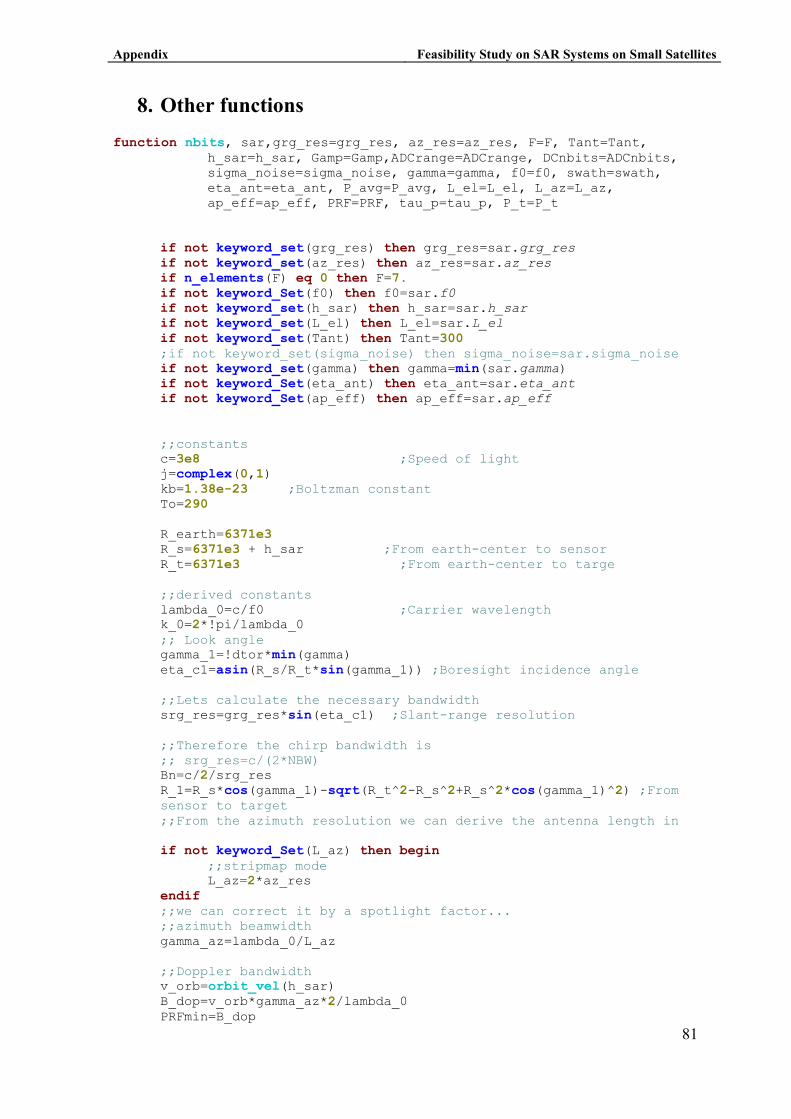
Appendix Feasibility Study on SAR Systems on Small Satellites
81
8. Other functions
function nbits, sar,grg_res=grg_res, az_res=az_res, F=F, Tant=Tant, h_sar=h_sar, Gamp=Gamp,ADCrange=ADCrange, DCnbits=ADCnbits, sigma_noise=sigma_noise, gamma=gamma, f0=f0, swath=swath, eta_ant=eta_ant, P_avg=P_avg, L_el=L_el, L_az=L_az, ap_eff=ap_eff, PRF=PRF, tau_p=tau_p, P_t=P_t if not keyword_set(grg_res) then grg_res=sar.grg_res if not keyword_set(az_res) then az_res=sar.az_res if n_elements(F) eq 0 then F=7. if not keyword_Set(f0) then f0=sar.f0 if not keyword_set(h_sar) then h_sar=sar.h_sar if not keyword_set(L_el) then L_el=sar.L_el if not keyword_set(Tant) then Tant=300 ;if not keyword_set(sigma_noise) then sigma_noise=sar.sigma_noise if not keyword_set(gamma) then gamma=min(sar.gamma) if not keyword_Set(eta_ant) then eta_ant=sar.eta_ant if not keyword_Set(ap_eff) then ap_eff=sar.ap_eff ;;constants c=3e8 ;Speed of light j=complex(0,1) kb=1.38e-23 ;Boltzman constant To=290 R_earth=6371e3 R_s=6371e3 + h_sar ;From earth-center to sensor R_t=6371e3 ;From earth-center to targe ;;derived constants lambda_0=c/f0 ;Carrier wavelength k_0=2*!pi/lambda_0 ;; Look angle gamma_1=!dtor*min(gamma) eta_c1=asin(R_s/R_t*sin(gamma_1)) ;Boresight incidence angle ;;Lets calculate the necessary bandwidth srg_res=grg_res*sin(eta_c1) ;Slant-range resolution ;;Therefore the chirp bandwidth is ;; srg_res=c/(2*NBW) Bn=c/2/srg_res R_1=R_s*cos(gamma_1)-sqrt(R_t^2-R_s^2+R_s^2*cos(gamma_1)^2) ;From sensor to target ;;From the azimuth resolution we can derive the antenna length in if not keyword_Set(L_az) then begin ;;stripmap mode L_az=2*az_res endif ;;we can correct it by a spotlight factor... ;;azimuth beamwidth gamma_az=lambda_0/L_az ;;Doppler bandwidth v_orb=orbit_vel(h_sar) B_dop=v_orb*gamma_az*2/lambda_0 PRFmin=B_dop
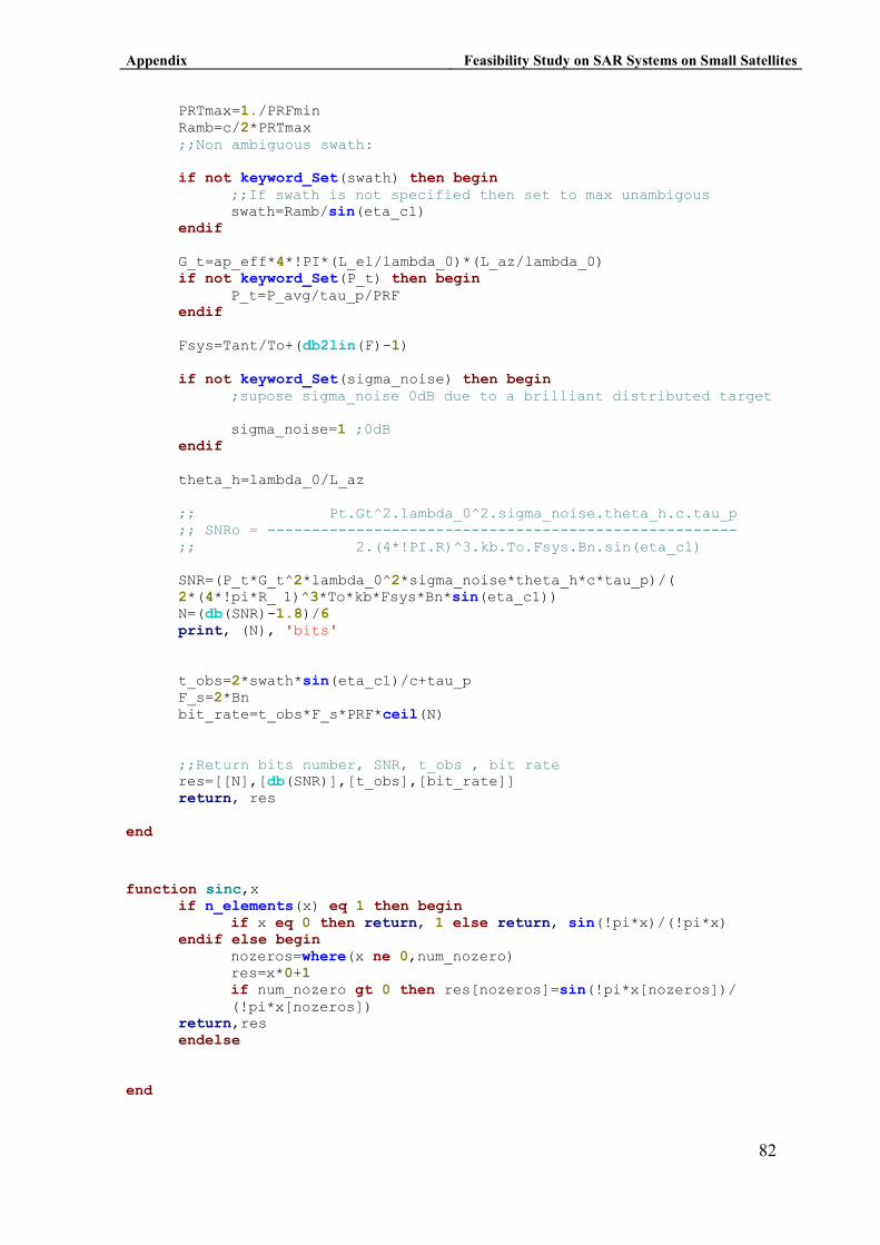
Appendix Feasibility Study on SAR Systems on Small Satellites
82
PRTmax=1./PRFmin Ramb=c/2*PRTmax ;;Non ambiguous swath: if not keyword_Set(swath) then begin ;;If swath is not specified then set to max unambigous swath=Ramb/sin(eta_c1) endif G_t=ap_eff*4*!PI*(L_el/lambda_0)*(L_az/lambda_0) if not keyword_Set(P_t) then begin P_t=P_avg/tau_p/PRF endif Fsys=Tant/To+(db2lin(F)-1) if not keyword_Set(sigma_noise) then begin ;supose sigma_noise 0dB due to a brilliant distributed target sigma_noise=1 ;0dB endif theta_h=lambda_0/L_az ;; Pt.Gt^2.lambda_0^2.sigma_noise.theta_h.c.tau_p ;; SNRo = ----------------------------------------------------- ;; 2.(4*!PI.R)^3.kb.To.Fsys.Bn.sin(eta_c1) SNR=(P_t*G_t^2*lambda_0^2*sigma_noise*theta_h*c*tau_p)/( 2*(4*!pi*R_ 1)^3*To*kb*Fsys*Bn*sin(eta_c1)) N=(db(SNR)-1.8)/6 print, (N), 'bits' t_obs=2*swath*sin(eta_c1)/c+tau_p F_s=2*Bn bit_rate=t_obs*F_s*PRF*ceil(N) ;;Return bits number, SNR, t_obs , bit rate res=[[N],[db(SNR)],[t_obs],[bit_rate]] return, res end
function sinc,x if n_elements(x) eq 1 then begin if x eq 0 then return, 1 else return, sin(!pi*x)/(!pi*x) endif else begin nozeros=where(x ne 0,num_nozero) res=x*0+1 if num_nozero gt 0 then res[nozeros]=sin(!pi*x[nozeros])/ (!pi*x[nozeros]) return,res endelse end
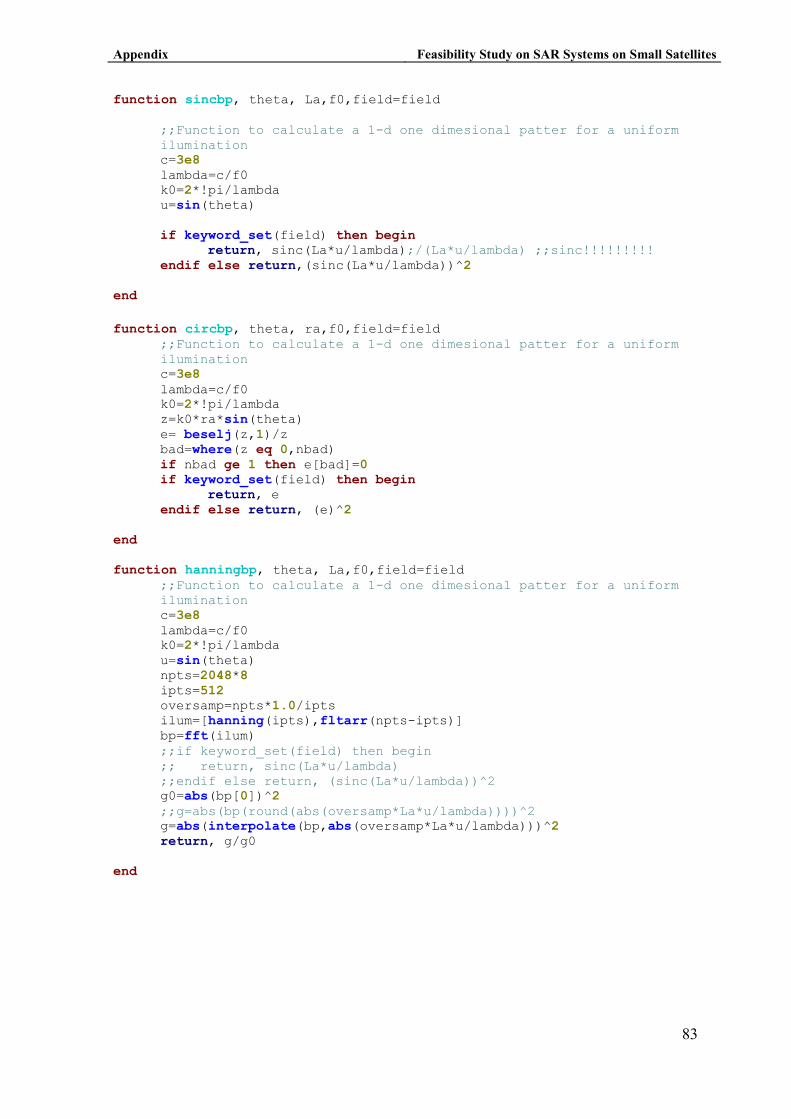
Appendix Feasibility Study on SAR Systems on Small Satellites
83
function sincbp, theta, La,f0,field=field ;;Function to calculate a 1-d one dimesional patter for a uniform ilumination c=3e8 lambda=c/f0 k0=2*!pi/lambda u=sin(theta) if keyword_set(field) then begin return, sinc(La*u/lambda);/(La*u/lambda) ;;sinc!!!!!!!!! endif else return,(sinc(La*u/lambda))^2 end
function circbp, theta, ra,f0,field=field ;;Function to calculate a 1-d one dimesional patter for a uniform ilumination c=3e8 lambda=c/f0 k0=2*!pi/lambda z=k0*ra*sin(theta) e= beselj(z,1)/z bad=where(z eq 0,nbad) if nbad ge 1 then e[bad]=0 if keyword_set(field) then begin return, e endif else return, (e)^2 end function hanningbp, theta, La,f0,field=field ;;Function to calculate a 1-d one dimesional patter for a uniform ilumination c=3e8 lambda=c/f0 k0=2*!pi/lambda u=sin(theta) npts=2048*8 ipts=512 oversamp=npts*1.0/ipts ilum=[hanning(ipts),fltarr(npts-ipts)] bp=fft(ilum) ;;if keyword_set(field) then begin ;; return, sinc(La*u/lambda) ;;endif else return, (sinc(La*u/lambda))^2 g0=abs(bp[0])^2 ;;g=abs(bp(round(abs(oversamp*La*u/lambda))))^2 g=abs(interpolate(bp,abs(oversamp*La*u/lambda)))^2 return, g/g0 end
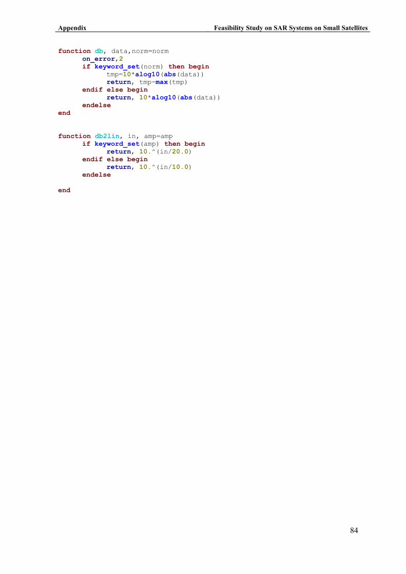
Appendix Feasibility Study on SAR Systems on Small Satellites
84
function db, data,norm=norm on_error,2 if keyword_set(norm) then begin tmp=10*alog10(abs(data)) return, tmp-max(tmp) endif else begin return, 10*alog10(abs(data)) endelse end function db2lin, in, amp=amp if keyword_set(amp) then begin return, 10.^(in/20.0) endif else begin return, 10.^(in/10.0) endelse end