August 2003

Leaders in Cutting Edge Technology

Software, Hardware and Services for The Engineering Community

LEAP

Australia Altair

Western Region US DYNAMAX

US Cril Technology

Simulation France

GISSETA

India MFAC Canada

DYNAmore Germany

Flotrend Taiwan

KOSTECH

Korea ERAB Sweden

THEME Korea

ALTAIR Italy

CAD-FEM Germany

Numerica SRL Italy

ANSYS China

Dr. Ted. Belytschko

US Dr. Bhavin V. Mehta

US Dr. Taylan Altan

US Dr. David Benson

US

Dr. Alexey L. Borovkov

Russia

Prof. Gennaro Monacelli

Italy

Prof. Ala Tabiei US

Articles

04 MSC.visualNastran 4D Improves Centrifugal Fan Design at Halifax Fans Ltd., UK 07 Website - Co-hosted Publication Sites for the LS-DYNA Engineering Community 08 FEA Information Participants 09 Special Announcements and Highlights of the News Page 10 INTEL Corporation Success Story 14 LS-DYNA User Conference Invitation 15 LS-OPT Section 2.6 Presentation Purdue University, CSD, Technical Report #03-011,2003 – Producing High-Quality

Visualizations of Large-Scale Simulations – Voicu Popescu, Chris Hoffman, CS – Sami Kilic, CRI – Mete Sozen, School of Civil Eng. – Scott Meador, ITaP Purdue University

Editor Trent Eggleston Editor – Technical Content Arthur B. Shapiro Technical Writer Dr. David Benson Technical Writer Uli Franz Graphic Designer Sandy Boling Graphic Designer Wayne Mindle Feature Director Marsha J. Victory

The contents of this publication is deemed to be accurate and complete. However, FEA Information Inc. doesn’t guarantee or warranty accuracy or completeness of the material contained herein. All trademarks are the property of their respective owners. This publication is published for FEA Information Inc., copyright 2003. All rights reserved. Not to be reproduced in hardcopy or electronic copy.

4

MSC.visualNastran 4D Improves Centrifugal Fan Design at Halifax Fans Ltd., UK Reprinted from Succcess Stories www.mscsoftware.com

© Copyright MSC Software, 2003

In 1965, Halifax Fan Ltd. was founded to serve local industryýs need for centrifugal fans. Today, almost 40 years later, Halifax Fan is one of the leading companies in the design, development and manufacture of centrifugal fans. These fans are now supplied to a wide range of industries around the world. Halifax Fan enjoys an excellent reputation, and the companyýs extensive customer list represents a comprehensive range of market sectors and applications, such as petrochemical, pharmaceutical, food, and power generation. Providing the highest quality product and customer service has always been of prime importance and a key factor in maintaining Halifax Fan's position at the forefront of fan technology. Since the companyýs founding, the development and design of fans has changed significantly, which consequently affects their design and production cycles. Halifax Fan used to employ an in-house Windows-based program to mechanically design and test products such as fan impellers. When production costs and time needed to be reduced and the design cycle shortened, Halifax Fan implemented MSC.visualNastran 4D in their design process. Within a 3D CAD environment, the required components are designed based on criteria such as volume, pressure and temperature, and then the design is validated by MSC.visualNastran 4D.

The Challenge: Aerofoil Blade Sections While Halifax Fan offers a broad range of standard products, a large proportion of their products are custom-designed to meet the many varied requirements of individual industry applications. In 2002, Halifax Fan undertook a feasibility study into aerofoil blade sections. The new sections required were different than the standard sections normally requested by clients and needed to be evaluated and analysed. Because the engineering techniques in place at the company did not provide a suitable understanding of the effects of the changes on these blades, other methods needed to be assessed. The engineers at Halifax Fan felt that a finite element analysis (FEA) program would yield quick and accurate results. Because they needed a software product they could easily combine with AutoCAD Mechanical Desktop, their 3D CAD software, MSC.visualNastran 4D, among others, was tested.

Today Halifax Fan uses MSC.visualNastran 4D mainly for the mechanical design of fan impellers and casings. In both applications, the design task is to optimise the strength of the components under operating conditions and to reduce the material needed in manufacturing the final product. With MSC.visualNastran 4D, Halifax engineers can predict the required thickness of the material and therefore reduce the material used in the final product.

5

Design Solutions with the co-operation of a student at Bradford University, writing his thesis on FEA software, MSC.visualNastran 4D was benchmarked against other software tools. Of primary importance to Halifax Fan was easy and accurate data exchange between the CAD and testing software without any loss of data, as well as the user-friendliness of the software. MSC.visualNastran 4D was found to be the best overall software package for Halifax Fan and was implemented into the design process. By using MSC.visualNastran 4D, Halifax Fan engineers were now able to use and test the already prepared 3D design of the impeller and the casing in a broader way. They could analyse the whole impeller as a complete assembly using the 3D CAD modelýs data, while with their previous design methods only one part could be analysed at a time and the interaction between parts was completely left to the judgement of the design engineers. The engineers were able to import the 3D model into MSC.visualNastran 4D, simulate the rotation speed of the impeller and then receive the results they needed to proceed with design and production. Thanks to MSC.visualNastran 4D, the Halifax Fan engineers gained greater confidence in their design and felt sure that they would design it right the first time, before actually building a physical prototype of the fan itself. As a consequence, new designs are being released 10% faster for manufacture. An All-Purpose Tool MSC.visualNastran 4D supports Halifax Fan in finding solutions for every type of fan, especially completely new fan types or critical designs ý for instance, as in the design of a fan case which needed to withstand an internal explosion. In this project, a standard 3D fan was modelled within the 3D software package, then analysed with the exact pressure the fan case would experience in case of an explosion. From this data, it was possible to predict the necessary material thickness, as well as the addition or removal of case stiffeners. Besides these examples, MSC.visualNastran 4D is widely used throughout the whole company. It has, for example, become an important tool in the Halifax Fan sales department: The company often bids for work covering one-off designs that are based on existing fan shapes. By using MSC.visualNastran4D, the assembly is designed with the Halifax fan CAD tool, then imported into 4D and tested before even writing the tender. This allows Halifax to offer a detailed and accurate bid for a product they already understand. In addition, Halifax Fan uses the visualisation aspects of MSC.visualNastran 4D for marketing purposes to demonstrate the company’s capabilities.

6

Conclusion: As existing techniques could not adequately cover the design of the aerofoil blade, Halifax Fans would have had to resort to physical testing to gain the knowledge for this one-off product. With MSC.visualNastran 4D, the need for building prototypes and testing was greatly reduced and Halifax Fan was able to improve the designs for a fraction of the cost on every contract. Due to the advanced technology of MSC.visualNastran 4D, Halifax Fan is able to produce products that are not over-engineered. This has led to a reduction of design and manufacturing time as well as to a reduction of the amount of material used. The thickness of the material used, as well as the correct type, can be predicted and tested virtually without the need to build a physical prototype. Thus, Halifax Fan has not only speeded up and improved their designs with MSC.visualNastran 4D, but also reduced the costs of the overall project. Implementing MSC.visualNastran 4D was part of the company’s strategy to maintain its position as a market leader through an ongoing investment programme. Halifax Fan plans to continue to use MSC.visualNastran 4D not only to improve their design and production process and in the areas of sales and research and development, but also for visualization capabilities in marketing. Displacement at Front Displacement at back

Computer Model of Entire Fan

7

Co-hosted Publications Sites for the LS-DYNA Engineering Community Brought to you by FEA Information Inc. (USA) and DYNAmore (Germany)

www.feapublications.com

www.dynalook.com

8

FEA Information Participants Commercial and Educational

Headquarters Company Australia Leading Engineering Analysis Providers www.leapaust.com.au Canada Metal Forming Analysis Corp. www.mfac.com China ANSYS – China www.ansys.com.cn France Cril Technology Simulation www.criltechnology.com Germany DYNAmore www.dynamore.de Germany CAD-FEM www.cadfem.de India GissEta www.gisseta.com Italy Altair Engineering srl www.altairtorino.it Italy Numerica srl www.numerica-srl.it Japan The Japan Research Institute, Ltd www.jri.co.jp Japan Fujitsu Ltd. www.fujitsu.com Japan NEC www.nec.com Korea THEME Engineering www.lsdyna.co.kr Korea Korean Simulation Technologies www.kostech.co.kr Russia State Unitary Enterprise - STRELA www.ls-dynarussia.com Sweden Engineering Research AB www.erab.se Taiwan Flotrend Corporation www.flotrend.com UK OASYS, Ltd www.arup.com/dyna USA INTEL www.intel.com USA Livermore Software Technology www.lstc.com USA Engineering Technology Associates www.eta.com USA ANSYS, Inc www.ansys.com USA Hewlett Packard www.hp.com USA SGI www.sgi.com USA MSC.Software www.mscsoftware.com USA DYNAMAX www.dynamax-inc.com USA AMD www.amd.com Educational Participants

USA Dr. T. Belytschko Northwestern University USA Dr. D. Benson Univ. California – San Diego USA Dr. Bhavin V. Mehta Ohio University USA Dr. Taylan Altan The Ohio State U – ERC/NSM USA Prof. Ala Tabiei University of Cincinnati Russia Dr. Alexey I. Borovkov St. Petersburg State Tech.

University Italy Prof. Gennaro Monacelli Prode – Elasis & Univ. of

Napoli, Federico II

9

Special Announcements and Highlights of News Pages

Posted on FEA Information and archived one month on the News Page July 07 AVI Library – AVI 25a Added USSID model AMD AMD Athlon™ XP-M processor up to 2400+ NEC Express5800/1080Rc MFAC Distributor in Canada July 14 AVI Library – AVI 200 CH-47 crash event ANSYS 2004 Conference Dynamax Distributor in US JRI JMAG-Studio SGI Silicon Graphics® Onyx4TM ERAB Distributor in Sweden July 27 ETA Corp. Profile Oaysis Primer Kostech Distributor in Korea

Events & Courses from the Events page on www.feainformation.com

2003

Oct 02-05 International Conference on CAE and Computational Technologies for Industry - Sardinia, Italy: info@consorziotcn.it

Oct 14-15

The Japan Research Institute LS-DYNA & JMAG Users Conference 2003 will be held at Akasaka Prince Hotel in Tokyo, Japan hosted by The Japan Research Institute. Contact : conf-info@sci.jri.co.jp

Oct 29-31 Hosted at the conveniently located Novi Expo Center in Detroit, Michigan, Testing Expo North America 2003 will bring together, under one roof, leading test equipment manufacturers and test service providers.

Nov 12-14 CAD-FEM User Conference 2003 - Dorint Sanssouci Hotel, Berlin Potsdam. Information will be posted soon

2004

May 2-3 8th International LS-DYNA Users conference will again be held at the Hyatt Regency Dearborn, Fairlane Town Center, Dearborn, MI hosted by LSTC and ETA

�

10

INTEL Corporation Success Story © Copyright, 2003 Intel Corporation

Excerpt from Cornell Theory Center Aricle. The full article can be read at: http://www.intel.com/ebusiness/casestudies/ctc/

Challenge: How can High-Performance Computing (HPC) users get the floating-point performance, large memories and memory bandwidth to meet their toughest challenges?

Solution: Capitalize on Intel® Architecture and the new Intel® Itanium® processor family. Cornell Theory Center* did, and saw a 340 percent speed-up in critical aspects of their teraflops-class materials science code. Intel®-based clusters are helping them solve more complex problems more quickly, collaborate more easily and ultimately accelerate the rate of scientific discovery and collaboration.

Understanding the Physics of Aging Airplanes: How long can an airplane remain in service? Aircraft cost millions to design and manufacture, so adding an extra year or two to an airplane's life can directly impact an aerospace company's bottom line. Yet no one wants to jeopardize safety by keeping a plane flying beyond its limits.

Materials Science and High-Performance Computing (HPC) solutions help make the call. And at one of the nation's leading HPC research centers, the breakthrough performance of Intel®-based clusters is enabling engineers and physicists to provide greater understanding and more nuanced answers to these and other Materials Science questions.

Manufactured products are made from materials—the metal and glass substances that have existed for eons, as well as state-of-the-art ceramics, plastics, semiconductors and more. Materials are so critical that past civilizations are known by the materials they used—think of the Stone Age, Bronze Age, Iron Age and so forth. Some experts assert that Materials Science is the most important engineering discipline today. From the computer industry (based largely on a single material&3151silicon) to new biotechnology materials that promise next-generation advances such as ceramic cement for bone repair or polymer-based tissue engineering, it's no exaggeration to say we live in a Material Age.

Materials Take Flight: Materials Science is a cornerstone technology for virtually all product design and manufacturing. At the start of the product life cycle, engineers analyze product requirements and determine what materials can fulfill them. At the other end of the life cycle, technologists use their knowledge of the properties and behavior of a product's component materials to help determine how long the product can remain viable. For aging aircraft fleets, materials scientists combine intense computer simulations with experimental data to predict how much longer an aircraft can safely fly.

"The average age of a commercial jet airliner is over 17 years, and the average plane in the U.S. Air Force fleet is 22 years old," says Anthony R. Ingraffea, professor of civil engineering at Cornell University*, associate director of the Cornell Theory Center* (CTC), and head of the Cornell Materials Institute* (CMI). "The materials in those airliners are being taxed to perform well beyond their originally intended design lives, and the airlines don't have an adequate way to predict the performance of those materials beyond the original intended life of these aircraft. In a sense, as the planes get older, they become flying test beds."

Ingraffea is part of a team of CMI engineers and physicists that's using powerful clusters based on the Microsoft* Windows* Advanced Server operating system and Intel® Pentium® III Xeon™ processors and Intel® Itanium® processors to determine how a minute fracture in an airplane's "skin" is likely to

11

spread and where and when it will likely rupture. Critical aspects of their sophisticated Crack Propagation on Teraflops Computers (CPTC) code have seen a speed-up of 3.42 times for single-processor execution on an Itanium-based system.

Cornell Theory Center: Solution

A Strategic Decision. The Cornell Theory Center is one of the U.S.’s premier research centers, making a mark as an early technology adopter and thought leader in HPC for both scientific and business end-users. The CTC was well ahead of the curve when it began investigating Windows-based* Intel® clusters for HPC in 1996 and deploying them in 1997. With the release of the Intel® Itanium® processor family in 2000, the rest of the industry is catching up—and CTC is firmly convinced that Intel Itanium architecture is an inflection point that will transform HPC solutions in both industry and academia.

"The Cornell Theory Center was the first in the world to go completely to an Intel® Architecture-based Microsoft* solution for high-performance computing," says Linda Callahan, executive director of the CTC. "At the time, people thought we were nuts. But we made a strategic decision, and we've proven that Intel delivers a highly effective and productive HPC architecture. Now we're at the forefront of a transition from proprietary RISC architectures to open clusters based on Intel Architecture and the Windows* 2000 operating system."

Meeting the Challenge. Cost was secondary, however, compared to the question of whether Intel-based clusters could handle some of the world's most demanding HPC applications. The answer has been a resounding yes.

"Our Windows and Intel powered clusters support the full range of large-scale HPC activities," says Callahan. "They consistently run at 99.999 percent reliability and higher, they're far easier to manage and maintain than traditional HPC systems, and their greater affordability and ease of use makes them very accessible. Every time we turn around, we're building a cluster for another group that wants to do high performance computing."

Today, CTC's results speak for themselves. All the Center's HPC resources run Windows and Intel Architecture, and the Center's flagship machine, Velocity*, is a Dell* cluster built on 64 four-way Pentium III Xeon processors. Velocity and CTC's other Intel-based clusters support HPC applications ranging from manufacturing optimization and engineering design, to bioinformatics and genome research, to financial risk analysis modeling. More than 600 users with an active technology exchange network, involving more than 80 companies and research institutions, utilize CTC resources and services and develop new HPC tools based on Intel Architecture and Microsoft Windows.

Financial modeling is an area of particular interest for CTC. Its Manhattan Center in New York uses Intel-based clusters to support a wealth of HPC services for financial institutions, helping them port their UNIX* codes to the Windows environment.

The Center is using Itanium-based workstations and has successfully piloted an Itanium-based cluster. CTC is also deploying the world's first Windows and Intel-based Computer Assisted Virtual Environment (CAVE*)-like facility. CAVE systems, originally developed at the University of Illinois, provide an immersive virtual reality room where technologists can interact with high-resolution 3D representations of their simulation results.

Solving More Complex Problems. The Intel Itanium architecture is a watershed for CTC and Ingraffea's fracture mechanics project—and, Ingraffea says, for science itself. The CPTC code is used by engineers and scientists at a variety of universities and National Science Foundation-funded

12

institutions. It’s designed for problems involving complex 3D geometries with arbitrary crack shape, multi-physics and non-linear system response. These problems are very demanding to simulate. For starters, the region being modeled grows as the crack grows and spreads. Even more challenging, the focus and scale of the simulation must shift as the simulation progresses. Floating-point accuracy is critical, and snapshots must be taken and data extracted at a number of different points during the process.

"For us to base our simulations on material behavior, starting from the atomic scale and working all the way up to the size of an aircraft, puts tremendous demands on the size, complexity and rigor of our simulations," Ingraffea says. "We need to be able to solve very large problems with very good physics, and that takes tremendous computer power."

This class of problem benefits tremendously from the Intel Itanium architecture, taking advantage of the dramatic increase in floating-point calculations and memory bandwidth, according to Ingraffea. Previously, CMI scientists needed to perform time-consuming, error-prone and non-portable fine-tuning to improve the ratio between floating point and load/store operations.

"Intel Itanium architecture is among the first to provide an instruction set architecture (ISA) with explicit support for the instruction-level and thread-level parallelism required to optimize CMI’s code," says Ingraffea. "As such, we can overcome critical performance bottlenecks."

Intel® Itanium® Architecture: Changing Science. Since moving to CTC’s new strategic applications cluster, Velocity+, at the beginning of 2001, CMI has dramatically increased the size and complexity of its typical problem. Simulations recently run on Velocity+ achieved almost 100 times greater resolution than on the Center’s previous UNIX system, and were performed in less than a tenth the time. And the Intel Itanium architecture opened the door for greater improvements.

"The Intel Itanium architecture is changing how science is done," says Ingraffea. "It enables us to bring better physics to bear and solve bigger pieces of the problem, still in an affordable fashion and a timely manner. It’s also ’democratizing’ research and accelerating the pace of scientific discovery. We’re able to bring more researchers to bear on a problem because we’re drastically reducing the cost of high-performance computing."

Itanium-based HPC systems are expanding the team’s vision of what it can accomplish. "Many important Materials Science problems have their origin with very, very small defects at the atomic scale," Ingraffea says. "It’s been a dream for two or three generations of researchers to bring together the basic physics and science of the atomic scale behavior of matter; then see how that information directly impacts a real life aerospace situation, such as how a wing on an aircraft performs or how the material in a gas turbine engine can withstand (or not withstand) tremendous heat and stress. Because of the tremendous computing power, affordability and universality of Intel-based clusters, we’re quickly approaching the ability to combine simulations in precisely this way."

CTC chief technology officer, David Lifka elaborates: "The fracture mechanics group has a goal of doing a problem of a million degrees of freedom with a thousand time steps in an hour," he says. "With Intel Architecture, we’ve been taking incremental steps forward. Now, with the Intel Itanium architecture, we expect to make leaps toward that goal. It’s very achievable and incredibly exciting."

13

Lessons Learned:

Ride the price/performance curve of mainstream computing. Moore’s Law and Intel’s commitment to maintaining it—offers HPC users a rapid path to on-going performance increases at affordable prices. The Intel® Itanium® processor family's Explicitly Parallel Instruction Computing (EPIC) architecture, high floating-point performance, 64-bit address space, large cache memories and excellent memory bus bandwidth, combined with performance-optimized Intel® compilers, can handle the toughest HPC challenges. The results: better science at a lower cost.

Make the most of volume economics. Microsoft* Windows* and Intel-based platforms let HPC users benefit from the thousands of tools, applications, devices and services available due to the pervasiveness of Intel Architecture in the marketplace. They also enable users to more easily collaborate with technologists from other companies and institutions since Intel Architecture is built on open industry standards.

Create a unified HPC environment of desktop-to-cluster scalability. A consistent environment reduces complexity and simplifies management. It also speeds development and allows users to move codes from their workstations to a cluster or virtual reality environment without a hitch.

Take advantage of Intel’s comprehensive HPC solutions. Intel offers more than just chips. It also delivers networking products, software, compilers, tools, middleware and services, not to mention powerful relationships with leading hardware, software and system integration vendors. CTC's fracture mechanics team used Intel's high performance C, C++ and Fortran compilers, which provide quadruple-precision 128-bit floating-point precision, as well as Intel® Math Kernel Libraries (MKL) and Intel® VTune™ Performance Analyzer. Members of the team also consulted with the Intel® Application Service Center engineers to learn how to take advantage of the new architecture and compilers.

The Intel® e-Business Network is one of the world's largest cooperative business communities all working with Intel products, technologies and services with a common goal of building better—more agile—e-Business solutions for you.

14

The 8th International LS-DYNA Users Conference

May 2nd – 4th, 2004 Invitation

Co-hosted by Livermore Software Technology Corp. (LSTC) - Engineering Technology Associates (ETA),

Conference Papers: The first named author of each accepted paper will receive a free admission to the conference, if the author registers at the hotel under LSTC Conference registration. Contact: vic@lstc.com for details.

* Aerospace * Automotive Crashworthiness * Ballistics and Penetration * Biomechanics * Civil Engineering * Impact and Drop Testing * Manufacturing Processes * Modeling Techniques * Metal Forming * Nuclear Applications * Occupant Safety * Offshore Applications * Seismic Engineering * Ship Building * Transportation * Virtual Proving Ground

Abstract Length Apprx. 300 words, please include figures if possible

Paper Length Maximum of 3,000 words, single-spaced, on 8-1/2" x 11" paper

Format A MS Word template will be provided

Contact papers@lstc.com - Dr. Wayne Mindle

Livermore Software Technology Corp. www.lstc.com

7373 Las Positas Road, Livermore, CA 94550 Tel: 925-449-2500

Engineering Technology Associates Inc. www.eta.com

1133 E. Maple, Troy, MI 48083 Tel: 248-729-3010

The 8th International LS-DYNA Users conference will again be held at the Hyatt Regency Dearborn Hotel & Conference Center, Fairlane Town Center, Dearborn, MI.

Abstract Deadline: December 5th

Notification: January 10th

Paper Deadline: March 5th

Contact: Marsha Victory vic@lstc.com �

Optimization Methodology Excerpt from LS-OPT User’s Manual

LS-OPT is free from LSTC

Sections 2.1 through 2.5.4 are published in FEA Information News February 2003

2.6 Experimental design

Experimental design is the selection procedure for finding the points in the design space that must be

analyzed. Many different types are available [34]. The factorial, Koshal, composite, D-optimal and Latin

Hypercube designs are detailed here.

2.6.1 Factorial design

This is an grid of designs and forms the basis of many other designs. is the number of grid points in

one dimension. It can be used as a basis set of experiments from which to choose a D-optimal design. In

LSOPT, the 3n and 5

n designs are used by default as the basis experimental designs for first and second

order D-optimal designs respectively.

n� �

Factorial designs may be expensive to use directly, especially for a large number of design variables.

2.6.2 Koshal design

This family of designs are saturated for modeling of any response surface of order d.

First order model

For n = 3, the coordinates are:

�

�

�

�

�

�

�

�

�

�

�

�

100

010

001

000

321 xxx

As a result, four coefficients can be estimated in the linear model

(2.18)T

nxx ],,,1[ 1 �=φ

Second order model

For n = 3, the coordinates are:

�

�

�

�

�

�

�

�

�

�

�

�

�

�

�

�

�

�

�

�

�

�

�

�

�

�

�

�

�

�

�

�

−−

−

110

101

011

100

010

001

100

010

001

000

321 xxx

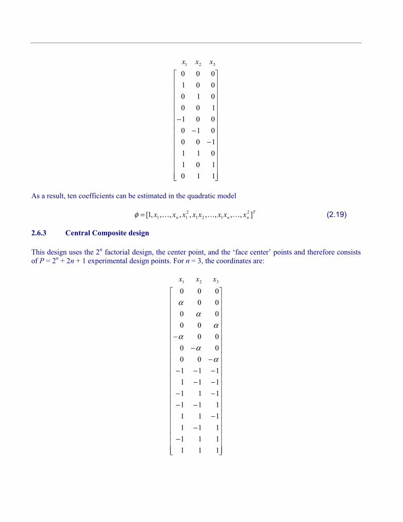
As a result, ten coefficients can be estimated in the quadratic model

(2.19)T

nnn xxxxxxxx ],,,,,,,,,1[ 2

121

2

11 ���=φ

2.6.3 Central Composite design

This design uses the 2n

factorial design, the center point, and the ‘face center’ points and therefore consists

of P = 2n + 2n + 1 experimental design points. For n = 3, the coordinates are:

�

�

�

�

�

�

�

�

�

�

�

�

�

�

�

�

�

�

�

�

�

�

�

�

�

�

�

�

�

�

�

�

�

�

�

�

�

�

�

�

�

�

�

�

�

�

�

�

−−

−−−

−−−−−−−

−−

−

111

111

111

111

111

111

111

111

00

00

00

00

00

00

000

321

αα

αα

αα

xxx

The points are used to fit a second-order function. The value of 4 2n=α .

2.6.4 D-optimal design

This method uses a subset of all the possible design points as a basis to solve

XXTmax .

The subset is usually selected from an -factorial design where is chosen a priori as the number of grid

points in any particular dimension. Design regions of irregular shape, and any number of experimental

points, can be considered [38]. The experiments are usually selected within a sub-region in the design space

thought to contain the optimum. A genetic algorithm is used to solve the resulting discrete maximization

problem. See References [34,55].

n� �

The numbers of required experimental designs for linear as well as quadratic approximations are

summarized in the table below. The value for the D-optimality criterion is chosen to be 1.5 times the Koshal

design value. This seems to be a good compromise between prediction accuracy and computational cost

[38]. The factorial design referred to below is based on a regular grid of 2n points (linear) or 3

n points

(quadratic).

Table 2-1: Number of experimental points required for experimental designs

Linear approximation Quadratic approximationNumber of

Variables n Koshal D-optimal Factorial Koshal D-optimal Factorial

Central

Composite

1 2 2 2 3 3 3 3

2 3 4 4 6 9 9 9

3 4 6 8 10 15 27 15

4 5 8 16 15 23 81 25

5 6 9 32 21 32 243 43

6 7 11 64 28 42 729 77

7 8 12 128 36 54 2187 143

8 9 14 256 45 68 6561 273

9 10 15 512 55 83 19683 531

10 11 17 1024 66 99 59049 1045

2.6.5 Latin Hypercube Sampling (LHS)

The Latin Hypercube design is a constrained random experimental design in which, for n points, the range

of each design variable is subdivided into n non-overlapping intervals on the basis of equal probability. One

value from each interval is then selected at random with respect to the probability density in the interval.

The n values of the first value are then paired randomly with the n values of variable 2. These n pairs are

then combined randomly with the n values of variable 3 to form n triplets, and so on, until k-tuplets are

formed.

Latin Hypercube designs are independent of the mathematical model of the approximation and allow

estimation of the main effects of all factors in the design in an unbiased manner. On each level of every

design variable only one point is placed. There are the same number of levels as points, and the levels are

assigned randomly to points. This method ensures that every variable is represented, no matter if the

response is dominated by only a few ones. Another advantage is that the number of points to be analyzed

can be directly defined. Let P denote the number of points, and n the number of design variables, each of

which is uniformly distributed between 0 and 1. Latin hypercube sampling (LHS) provides a P-by-n matrix

S = Sij that randomly samples the entire design space broken down into P equal-probability regions:

( ) PS ijijij ζη −= , (2.20)

where are uniform random permutations of the integers 1 through P and independent random

numbers uniformly distributed between 0 and 1. A common simplified version of LHS has centered points

of P equal-probability sub-intervals:

Pjj ηη ,,1 � ijζ

( ) PS ijij 5.0−= η (2.21)

LHS can be thought of as a stratified Monte Carlo sampling. Latin hypercube samples look like random

scatter in any bivariate plot, though they are quite regular in each univariate plot. Often, in order to generate

an especially good space filling design, the Latin hypercube point selection S described above is taken as a

starting experimental design and then the values in each column of matrix S is permuted so as to optimize

some criterion. Several such criteria are described in the literature.

Maximin

One approach is to maximize the minimal distance between any two points (i.e. between any two rows of

S). This optimization could be performed using, for example, Simulated Annealing (see Appendix E). The

maximin strategy would ensure that no two points are too close to each other. For small P, maximin distance

designs will generally lie on the exterior of the design space and fill in the interior as P becomes larger. See

section 2.6.6for more detail.

Centered L2-discrepancy

Another strategy is to minimize the centered L2-discrepancy measure. The discrepancy is a quantitative

measure of non-uniformity of the design points on an experimental domain. Intuitively, for a uniformly

distributed set in the n-dimensional cube nI = [0,1]n, we would expect the same number of points to be in

all subsets of nI having the same volume. Discrepancy is defined by considering the number of points in

the subsets of nI . Centered L2 (CL2) takes into account not only the uniformity of the design points over

the n-dimensional box region nI , but also the uniformity of all the projections of points over lower-

dimensional subspaces:

( )

.22

5.0

2

5.01

1

2

5.0

2

5.01

2)1213(

1 1 12

1 1

2

2

2

� � ∏�

�

�

�

�

�

�

� −−

−+

−++

� ∏�

�

�

�

�

�

�

� −−

−+−=

= = =

= =

Pk Pi nj

ijkjijkj

Pi nj

ijijn

SSSS

P

SS

PCL

� � �

� �

(2.22)

2.6.6 Space-filling designs*

In the modeling of an unknown nonlinear relationship, when there is no persuasive parametric regression

model available, and the constraints are uncertain, one might believe that a good experimental design is a set

of points that are uniformly scattered on the experimental domain (design space). Space-filling designs

impose no strong assumptions on the approximation model, and allow a large number of levels for each

variable with a moderate number of experimental points. These designs are especially useful in conjunction

with nonparametric models such as neural networks (feed-forward networks, radial basis functions) and

Kriging, [60,62]. Space-filling points can be also submitted as the basis set for constructing an optimal (D-

Optimal, etc.) design for a particular model (e.g. polynomial). Some space-filling designs are: random Latin

Hypercube Sampling (LHS), Orthogonal Arrays, and Orthogonal Latin Hypercubes.

The key to space-filling experimental designs is in generating 'good' random points and achieving

reasonably uniform coverage of sampled volume for a given (user-specified) number of points. In practice,

however, we can only generate finite pseudorandom sequences, which, particularly in higher dimensions,

can lead to a clustering of points, which limits their uniformity. To find a good space-filling design is a

nonlinear programming hard problem, which – from a theoretical point of view – is difficult to solve

exactly. This problem, however, has a representation, which might be within the reach of currently available

tools. To reduce the search time and still generate good designs, the popular approach is to restrict the

search within a subset of the general space-filling designs. This subset typically has some good 'built-in'

properties with respect to the uniformity of a design.

The constrained randomization method termed Latin Hypercube Sampling (LHS) and proposed in [30], has

become a popular strategy to generate points on the 'box' (hypercube) design region. The method implies

that on each level of every design variable only one point is placed, and the number of levels is the same as

the number of runs. The levels are assigned to runs either randomly or so as to optimize some criterion, e.g.

so that the minimal distance between any two design points is maximized ('maximin distance' criterion).

Restricting the design in this way tends to produce better Latin Hypercubes. However, the computational

cost of obtaining these designs is high. In multidimensional problems, the search for an optimal Latin

hypercube design using traditional deterministic methods (e.g. the optimization algorithm described in [36])

may be computationally prohibitive. This situation motivates the search for alternatives.

Probabilistic search techniques, simulated annealing and genetic algorithms are attractive heuristics for

approximating the solution to a wide range of optimization problems. In particular, these techniques are

frequently used to solve combinatorial optimization problems, such as the traveling salesman problem.

Morris and Mitchell [33] adopted the simulated annealing algorithm to search for optimal Latin hypercube

designs.

In LS-OPT, space-filling designs can be useful for constructing experimental designs for the following

purposes:

1. The generation of basis points for the D-optimality criterion. This avoids the necessity to create a

very large number of basis points using e.g. the full factorial design for large n. E.g. for n=20 and 3

points per variable, the number of points = 320

3.5*109.

2. The generation of design points for all approximation types, but especially for neural networks for

which the D-Optimality criterion is currently not available.

3. The augmentation of an existing experimental design. This means that points can be added for each

iteration while maintaining uniformity and equidistance with respect to pre-existing points.

LS-OPT contains 6 algorithms to generate space-filling designs (see Table 2.2). Only Algorithm 5 has been

made available in the graphical interface. LS-OPTui.

Figure 2-1: Six space-filling designs: 5 points in a 2-dimensional box region

Table 2-2: Description of space-filling algorithms

Algorithm

Number

Description

0 Random

1 'Central point' Latin Hypercube Sampling (LHS) design with random

pairing

2 'Generalized' LHS design with random pairing

3 Given an LHS design, permutes the values in each column of the LHS

matrix so as to optimize the maximin distance criterion taking into account

a set of existing (fixed) design points. This is done using simulated

annealing. Fixed points influence the maximin distance criterion, but are

not allowed to be changed by Simulated Annealing moves.

4 Given an LHS design, moves the points within each LHS subinterval

preserving the starting LHS structure, optimizing the maximin distance

criterion and taking into consideration a set of fixed points.

5 given an arbitrary design (and a set of fixed points), randomly moves the

points so as to optimize the maximin distance criterion using simulated

annealing (see Appendix E).

Discussion of algorithms

The Maximin distance space-filling algorithms 3, 4 and 5 minimize the energy function defined as the

negative minimal distance between any two design points. Theoretically, any function that is a metric can be

used to measure distances between points, although in practice the Euclidean metric is usually employed.

The three algorithms, 3, 4 and 5, differ in their selection of random Simulated Annealing moves from one

state to a neighboring state. For algorithm 3, the next design is always a 'central point' LHS design (Eq.

2.21). The algorithm swaps two elements of I, Sij and Skj, where i and k are random integers from 1 to N, and

j is a random integer from 1 to n. Each step of algorithm 4 makes small random changes to a LHS design

point preserving the initial LHS structure. Algorithm 5 transforms the design completely randomly - one

point at a time. In more technical terms, algorithms 4 and 5 generate a candidate state, , by modifying a

randomly chosen element Sij of the current design, S, according to:

S ′

(2.23)ξ+=′ijij SS

where is a random number sampled from a normal distribution with zero mean and standard deviation

∈ [ min, max]. In algorithm 4 it is required that both and in Eq. (2.23) belong to the same Latin

hypercube subinterval.

ijS ′ijS

Notice that maximin distance energy function does not need to be completely recalculated for every iterative

step of simulated annealing. The perturbation in the design applies only to some of the rows and columns of

S. After each step we can recompute only those nearest neighbor distances that are affected by the stepping

procedures described above. This reduces the calculation and increased the speed of the algorithm.

To perform an annealing run for the algorithms 3, 4 and 5, the values for Tmax and Tmin can be adapted to the

scale of the objective function according to:

(2.24)ETT ∆×= maxmax :

ETT ∆×= minmin :

where E > 0 is the average value of |E'-E| observed in a short preliminary run of simulated annealing and

Tmax and Tmin are positive parameters.

The basic parameters that control the simulated annealing in algorithms 3, 4 and 5 can be summarized as

follows:

• Energy function: negative minimal distance between any two points in the design.

• Stepping scheme: depends on whether the LHS property is preserved or not.

• Scalar parameters:

1. Parameters for the cooling schedule:

- scaling factor for the initial (maximal) temperature, Tmax, in (2.24)

- scaling factor for the minimal temperature, Tmin, in (2.24),

- damping factor for temperature, µT, in (Eq. (E.5),

- number of iterations at each temperature, T (Appendix E)

2. Parameters that control the standard deviation of in (2.23):

- upper bound, max,

- lower bound, min.

3. Termination criteria:

- maximal number of energy function evaluations, Nit.

2.6.7 Random number generator

A portable random number generator is used for the construction of D-optimal designs (using the genetic

algorithm) and to generate Monte Carlo designs such as the Latin Hypercube. The algorithm employs a

scheme by Bays and Durham, as described in Knuth [24], and resembles the Maclaren-Marsaglia method. It

greatly increases the period of the basic linear congruential generator.

1

Purdue University Computer Science Dept. Tech Report 03-011

Producing High-Quality Visualizations of Large-Scale Simulations

Voicu Popescu, Chris Hoffmann, CS Sami Kilic, Computing Research Institute, Mete Sozen, CE

Scott Meador, ITaP Purdue University

Abstract

This paper describes the work of a team of researchers in computer graphics, geometric computing, and civil engineering to produce a visualization of the September 2001 attack on the Pentagon. The immediate motivation for the project was to understand the behavior of the building under the impact. The longer term motivation was to establish a path for producing high-quality visualizations of large scale simulations.

The first challenge was managing the enormous complexity of the scene to fit within the limits of state-of-the art simulation software systems and supercomputing resources. The second challenge was to integrate the simulation results into a high-quality visualization. To meet this challenge, we implemented a custom importer that simplifies and loads the massive simulation data in a commercial animation system. The surrounding scene is modeled using image-based techniques and is also imported in the animation system where the visualization is produced.

A specific issue for us was to federate the simulation and the animation systems, both commercial systems not under our control and following internally different conceptualizations of geometry and animation. This had to be done such that scalability was achieved. The reusable link created between the two systems allows communicating the results to non-specialists and the public at large, as well as facilitating communication in teams with members having diverse technical backgrounds.

CR Categories and Subject Descriptors: I.3.3 [Computer Graphics]: Applications, Three-dimensional Graphics and Realism, Graphics Utilities. I.6. [Simulation and Modeling]: Applications, Model Validation and Analysis, Output Analysis.

1. INTRODUCTION

1.1 Problem description Since Ken Wilson’s articulation of simulation as third paradigm of science in the mid-1980s [14], co-equal with experimental and theoretical science, simulations have become essential tools in many fields of science and engineering. Scientific simulations are used to crash-test an automobile before it is built, to study the interaction between a hip implant and the femur, to evaluate and renovate medieval bridges, to assess the effectiveness of

electronic circuit packaging by running circuit-board drop tests, or to build virtual wind tunnels.

In particular, finite-element analysis (FEA) plays a fundamental role in engineering because of its ability to integrate multiple physical phenomena, such as fluid flow, fluid/solid interaction, and material behavior. FEA systems compute a variety of physical parameters over the time span of the simulation, such as position, velocity, acceleration, stress, and pressure. The visual presentation of the results is either handed off to generic post-processors or else is studied in specific contexts in the field of scientific visualization.

Three dimensional computer graphics has advanced tremendously, driven mostly by the popularity of its applications in entertainment. Consumer-level priced personal computers with add-in graphics cards can produce high-quality images of complex 3D scenes at interactive rates or can run sophisticated animation software systems to produce, off-line, video sequences that very closely approach photorealism. Because of the specifics of the applications that commissioned their development, animation systems are mainly concerned with minimizing the production effort and maximizing the entertainment value of animations. They focus on the rendering quality, on the expressivity of the animated characters and are less concerned with closely following the laws of physics.

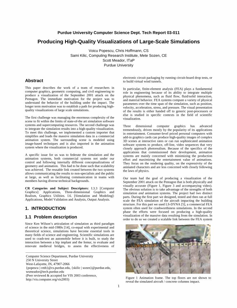
Our team had the goal of producing a visualization of the September 2001 attack on the Pentagon that is both physically and visually accurate (Figure 1, Figure 3 and accompanying video). The obvious solution is to take advantage of the strengths of both simulation and animation systems. The project had two distinct parts. During the first part we designed, tested and then ran at full scale the FEA simulation of the aircraft impacting the building structure. For this part we used LS-DYNA [5], a commercial FEA system often used for crashworthiness simulations. In the second phase the efforts were focused on producing a high-quality visualization of the massive data resulting from the simulation. In order to do so we created a scalable link between the FEA system

Computer Science Department, Purdue University 250 N University Street West-Lafayette, IN, 47907-2066 {popescu | cmh}@cs.purdue.edu, {skilic | sozen}@purdue.edu, wsmeador@tech.purdue.edu (Peer reviewed & accepted for VIS 2003 conference, http://vis.computer.org/vis2003) Figure 1 Animation frame. The top floors are not shown to

reveal the simulated aircraft / concrete columns impact.

2

and a commercial animation system (3ds max [19]). The link can be directly reused to create animations with physical fidelity regardless of the scientific or engineering domain.

1.2 Motivation A high-quality visualization of the results of a simulation first requires that the objects whose interaction is simulated be rendered using state-of-the-art rendering techniques. The second requirement is that the simulation be placed in the context of the immediate surrounding scene. For this the scene has to be modeled and rendered along with the simulation results.

Such a visualization makes the results and conclusions of the simulation directly accessible to others than the specialists that designed the simulation, without sacrificing scientific accuracy. This will make scientific simulations powerful tools that will routinely be used in a variety of fields including national security, emergency management, forensic science, and media.

A good visualization ultimately leads to improvements of the simulation itself. High-quality images quickly reveal discrepancies with experimental data observed over the years or recorded specifically for fine tuning the current simulation.

1.3 Process overview Figure 2 gives an overview of the process that converted the heterogeneous data documenting the event into the desired visualization.

The first step in creating the simulation was to generate the element meshes suitable for FEA. To keep the scene complexity within manageable limits, only the most relevant components of the aircraft and of the building were meshed. Then, the material model parameters were tuned during test simulations to achieve correct load deflection behavior. The FEA code was run on the full resolution meshes to simulate the first 250 milliseconds of the impact over 50 states.

The visualization part of the project began with modeling the Pentagon building from architectural blueprints using a CAD tool. The geometric model of the building and the surroundings were enhanced with textures projected from high-resolution satellite and aerial imagery using a custom tool. The 3ds max aircraft model used for visualizing the approach was readily available. The 3.5 GB of state data describing the mesh deformations was simplified, converted and imported into the animation system through a custom plugin. The imported meshes were aligned with the surrounding scene and enhanced with rendering material properties. Finally the integrated scene was rendered from the desired camera paths.

Prior work is discussed next. The remainder of the paper is organized as follows. Section 3 describes the simulation; section 4describes modeling the part of the scene not involved in the simulation; section 5 covers importing the simulation data into the animation system. Results are presented for each section separately. All the timing data was obtained on Pentium 4 Xeon, 2 GHz, 2 GB workstations. Discussion and directions for future work conclude the paper.

2. PRIOR WORK

Baker et al. [1] describe the simulation of a bomb blast and its impact on a neighboring building. The scenario investigated matches the 1996 attack on the Khobar towers. Two computational codes were used. The blast propagation was computed using CTH [3] at the Army’s research lab in Vicksburg [6]. Results of the CTH calculation are used as initial pressure loadings on the buildings and Dyna3D [4] is then used to model the structural response of the building to the blast. The results were visualized in the Dyna3D postprocessor and VTK (visualization toolkit [7]) using standard visualization techniques such as slicing and isosurfacing. The researchers report the difficulty of visualizing the large data sets; the solutions employed are reducing resolution, decimation and extraction of regions of interest. Enhancing the quality of the visualization using photographs is mentioned as future work.

A considerable body of literature in nuclear engineering is dedicated to simulating the crash of an aircraft into a concrete structure. Provisions for aircraft impact on reinforced concrete structures are incorporated into the Civil Engineering codes used for the design of nuclear containment structures. A full-scale test was conducted by Sugano et al. [2] to measure the impact force exerted by fighter aircraft (F-4D) on a reinforced concrete target slab. The study provided important information on the deformation and disintegration of the aircraft. A simplified computational model was also developed in order to capture the global response of the impact. This study provided us the experimental evidence that the airframe and the skin of the aircraft alone are not likely to cause the major damage on reinforced concrete targets.

To place the simulation in context we had to model and render the surroundings of the Pentagon. Research in image-based rendering (IBR) has produced several successful approaches for rendering

Figure 2 Process overview.

Figure 3 Visualization of the jet fuel.

3

complex large-scale natural scenes. The QuicktimeVR [9] system models the scene by acquiring a set of overlapping same-center-of-projection photographs that are stitched together to form panoramas. During rendering the desired view is confined to the centers of the panoramas. In our case it was important to allow for unrestrained camera motion so we dismissed the approach.

Image-based rendering by warping (IBRW) [10] relies on images enhanced with per-pixel depth. The depth and color samples are 3D warped (reprojected) to create novel views. Airborne LIDAR sensors can provide the depth data at appropriate resolution and precision. In the case of our project no depth maps of the Pentagon scene were available and we could not use IBRW. In light field rendering the scene is modeled with a database containing all rays potentially needed during rendering. The method does not scale well: the number of images that need to be acquired and the ray database grow to impractical sizes for large-scale scenes.

An approach frequently used for modeling large urban scenes combines images with coarse geometry into a hybrid representation. A representative example is the Façade system [11] which maps photographs onto buildings modeled with simple primitive shapes. The system was used to model and realistically render a university campus environment. The relatively simple geometry of the Pentagon building and the availability of photographs of the area motivated us to choose a hybrid geometry / images approach as described in section 4.

3. LARGE SCALE SIMULATION

FEA codes are among the most flexible and competent tools for simulating physical phenomena. A simulation is described by providing a geometric description, a set of constitutive models that capture non-linear material behavior, initial conditions, and the interaction of various components of the model through contact algorithms. The geometric description is in terms of nodes (points in 3-space) and elements (beam, shell and volume) partitioning the geometric objects. The elements have associated material properties that describe their behavior under strain. The simulation code integrates differential equations that express the material characteristics and the interaction and energy exchange between materials in contact (or in a field). Failure of elements in the simulation is achieved by imposing a maximum strain limit in the material model, and eroding elements that reach the limit. These elements are not considered in the dynamic equilibrium of

the model in the following time steps. Physically this means that the material tears or breaks at that locale. This approach enables the wings to cut through the reinforced concrete columns. Erosion of elements is a technique that is essential for simulating penetration problems.

Based on careful consideration, our simulation hypothesis is that the most massive structure, causing the bulk of the damage through its kinetic energy, has been the liquid fuel (kerosene) in the tanks of the aircraft. At impact, the plane was carrying an estimated 5,200 gallons of fuel and had a speed estimated at 480 mph. Damage inspection revealed that the performance of the building depended crucially on the spirally reinforced concrete columns of the building.

Accordingly we concentrated on modeling the columns and the fuel. This focus may come as a surprise. However, experimental research has given evidence that the airframe is not very strong in a head-on crash [2].

Figure 4 shows the finite element mesh (FEM) for the spirally reinforced concrete columns. We modeled the confined concrete core, the steel rebars, and the unconfined concrete cover (fluff). The column hexahedral elements are 7.5 x 7.5 x 15 cm in size. The column is anchored by the floor and ceiling supports (red in the figure). The fuel was modeled using an Arbitrary Lagrangian-Eulerian (ALE) formulation that integrates the Navier-Stokes equations of fluid dynamics for the motion of the liquid fuel. The Eulerian mesh is able to expand in order to enclose the splashing liquid fuel. Automatic mesh motion is achieved by following the mass-weighted average velocity of the ALE mesh. The fuel is specified in the Eulerian mesh in terms of per-cell fractional occupancy values. Figure 5 shows the liquid in the initial configuration. The Eulerian mesh elements are 15 x 15 x 15 cm in size.

A 3ds max model of the Boeing 757 was obtained from a game company [15] and formed the basis for creating the FEM of the plane. The meshed model includes fuselage

stringers reinforcing the body of the plane and ribs in the wing structure, as well as the fuselage floor. Those are the

structural elements of the plane deemed to be most significant. Our custom mesh generation tool uses a set of hard points in the wings and the

Figure 4 column FEM.

Figure 5 Eulerian mesh cells with >25% liquid occupancy.

Figure 6 Test simulation for tuning column / liquid interaction.

4

body. The mesh generation is parametric, which allows for conveniently generating meshes at various resolutions. We tried unsuccessfully to get a fully meshed model from Boeing. However, Boeing did share general structural characteristics of its aircraft with us which, in combination with literature on aircraft design, confirmed that the elements we had selected were the significant structural element relevant to the problem.

In order to calibrate the columns used in the simulation, a reinforced concrete column was analyzed under impact loading. Figure 6 (top) shows the calibration column subjected to high-speed impact with liquid. The liquid mass was idealized as a block (shown in red color). Figure 6 (bottom) illustrates the damaged state of the column after impact. Erosion of elements in the column allowed us to model penetration of the fluid and the splitting of the column into two pieces after impact. Different failure strain limits were used for the unconfined fluff cover and the confined concrete inner core. The steel rebars were also assigned failure strain limits in order to model the rupture behavior of the reinforcement.

The mesh density balances accuracy and model size to maximize resolution and fidelity while staying within software and hardware limitations. At 1.2 M nodes, the simulation took approximately 6 hours per recorded state on an IBM Power-4 platform with 8 processors and 64 GB of memory. The integration step size was 0.1 milliseconds, and we recorded 50 states, 5 milliseconds apart. The disk size of each state is 70 MB, for a total of 3.5 GB.

4. SURROUNDING SCENE

We decided to model the surrounding scene for two reasons. First we wanted to visualize the trajectory of the plane immediately before the collision. Second, we wanted to place the simulation results in context to make it easily understood by someone who was not closely involved with the investigation.

As described earlier, our approach was dictated by the available data documenting the scene. From the architectural blueprints we produced a CAD model of the building. The damage in the collapsed area was modeled by hand to match available photographs. The region surrounding the Pentagon was simply modeled with a large plane. The geometric models were enhanced with color using high-resolution satellite [16] and aerial imagery [8].

In order to apply a photograph to a geometric model two problems need to be solved. First one has to find the pose of the camera in a model-defined coordinate system (camera matching). Second the photograph pixels need to be mapped to the model triangles that are visible to the camera (projective texture mapping [17]). The basic functionality is available in animation systems such as 3ds max and Maya. We decided to implement our own camera matching / projective texture mapping tool to have more control over the camera matching and to create a conventionally texture mapped model. Such a model with individually texture mapped triangles can then be easily combined with other models (namely the approaching aircraft and the results of the simulation) and allows using multiple reference photographs with good control over the triangle to photograph assignment.

We find the camera pose using correspondences between the photograph and the geometric model. Since the camera used to take the photographs is not available we also calibrate for the focal length. The focal length is the only intrinsic parameter of the camera model used: the center of projection is assumed to project

in the center of the pixel grid, the pixels are assumed to be square and the lens distortion is ignored. We use this idealized model since the scene is flat (the height of the Pentagon building is small compared to its horizontal dimensions) and nearly coplanar points make the calibration for complex camera models numerically unstable. We search for the seven unknowns using the downhill simplex method. The starting position is obtained by rendering the model and manually adjusting the view such that the rendered image roughly matches the photograph. Convergence is achieved in negligible time. For a 3000 x 2000 pixels image the camera matching error is on average 3.5 pixels for 10 correspondences.

Once the view is known, the camera is transformed in a projector and the photograph pixels are deposited on the surface of the triangles to create individual texture maps. The algorithm proceeds as follows (Pseudocode 1). IB stores the IDs of the triangles that are seen by the photograph.

A texture map is generated for each visible triangle. The texture is aligned with the longest edge of the projected triangle and with its corresponding height. The lengths of the two segments in pixels give the texture resolution. By choosing the resolution this way, the texture subsamples the photograph in the part of the triangle near the camera and supersamples it at the far end. Subsampling implies losing some of the color information of the photograph. We have experimented with setting the texture resolution to the maximum sampling rate encountered at the near end of the triangle. The Pentagon building model contains long triangles and the conservative resolution produced excessively large textures. Using the z buffer the texture is set only for the part of the triangle actually seen in the photograph. This is important when other images are used to complete the texture of the triangle. To correctly handle triangles that have a thin projection, the texels traversed by the edges are set the same way (without the triangle membership test).

The building and ground plane model consisting of 25 K triangles was sprayed with a 3000 x 2000 pixels photograph. The resulting texture mapped model produced realistic visualizations of the Pentagon scene. Figure 8 shows an image rendered from a considerably different view than

Render model from camera view CV in item buffer IB and z buffer ZBFor each triangle T in IB Project T in CV Find longest edge e, corr. height h Allocate e x h texture map TM Set texture coordinates for T For each texel t in TM If t outside T continue Project t in CV at p If hidden by ZB continue Set t to photograph pixel p Set edge texels

Pseudocode 1 Texture generation

Figure 7 Photograph

Figure 8 Image rendered from texture mapped model

5

the view of the reference photograph, which is shown in Figure 7. The total disk size of the texture files is 160 MB. The difference when comparing to the 24 MB of the reference photograph is due to the texels outside of the triangle, to the texels corresponding to the hidden part of the triangle, to the thin triangles that have a texture larger than their area and to our simple merging of individual texture images that vertically collates 10 images to reduce the number of files. For now we rendered the scene offline so the large total texture size was not a concern. For real time rendering, the texture size has to be reduced. A simple greedy algorithm for packing the textures involving shifts and rotations is likely to yield good results. The rotation can be propagated upstream to the spraying to avoid the additional resampling.

5. INTEGRATION

The simulation results files are directly imported in 3ds max via a custom plugin. The 954 K nodes of the FEM define 355 K hexahedral (solid) elements used to model the column core and the fluff, 438 K hexahedral elements for the liquid elements, 15 K quadrilateral (shell) elements used to define the fuselage and floor of the aircraft, and 61 K segment (beam) elements used to define the ribs and stringers of the aircraft. The importer subdivides the simulation scene into objects according to materials to facilitate assigning rendering materials.

5.1 Solid objects Ignoring the liquid for now, the 12, 2 and 1 triangles per solid, shell and beam elements respectively imply about 4.3 M triangles for the solid materials in the simulation scene. This number is reduced by eliminating internal faces, which are irrelevant during rendering. An internal face is a face shared by two hexahedral elements. Because elements erode, faces that are initially internal can become visible at the fracture area. For this an object is subdivided according to the simulation states; subobject k groups all the elements that erode at state k. Discarding the internal faces of each subobject is done in linear time using hashing. This reduces the number of triangles to 1.3 M, which is easily handled by the animation system.

However, importing the mesh deformation into the animation system proved to be a serious bottleneck. The mesh deformations are saved by the FEA code as node positions at every state. The animation system supports per vertex animation but creating 50 position controllers for each of the remaining 700 K nodes takes days and the resulting scene file is unusable. The practical limit on the number of animation controllers is about 1 M. The number of animation controllers is reduced in two ways. First, the importer does not animate nodes with a total movement (sum of state to state movement) below a user chosen threshold (typical value 1 cm). Second, the trajectories of each node are simplified independently by eliminating (i.e. not creating) controllers for the nearly linear parts. We have experimented with two ways of simplifying the trajectory. In the first approach, a controller is removed if the resulting trajectory is, at every state, within a threshold (typical value 1 cm) of the original trajectory. This enforces the threshold globally at the cost of an order Ns2 running time where N is the number of nodes and s is the number of states. Our second approach considers triples of states A, B, C and removes the controller for B if B is closer than 1 cm from the line AC. The next triple considered is A, C, D if B is removed and B, C, D if not. When the threshold is considerably less than the amount a node moves between states, the result is virtually the same as in the case of the first approach, with the benefit of an order Ns running time. After simplification, 1.8 M controllers

remained. We distributed the simulation scene over three files, each covering one third of the simulation. Materials and cameras can of course easily be shared among several files. Importing the solid objects takes 2 hours total, out of which 1 hour is needed for the third part of the simulation. Once the solid objects are loaded, the animator assigns them standard 3ds max materials.

5.2 Liquid objects The liquid data saved at every state contains the position of the nodes of the Eulerian mesh and the fractional occupancy values at that state. The liquid could be directly rendered from the occupancy data using volume rendering techniques. We chose to build a surface boundary representation first in order to take advantage of the rendering capabilities of the animation system. For every state the importer selects the Eulerian mesh elements that have a liquid occupancy above a certain threshold (typical value 25%). The internal faces are eliminated similarly to the solid object case. Once the liquid is imported, two 3dsmax modifiers are applied. For now the modifiers are applied manually by the animator; in the future this step will be moved inside the importer. The first is the "relax" modifier, which changes the apparent tension of the surface by moving vertices toward an average center point. By relaxing the mesh, it rounds the edges without adding or removing faces. After relaxing the mesh, a "smooth" modifier is added to average the object's normals, which creates a surface that reacts well to light, reflection, and refraction.

Figure 9 Fuel rendered in animation system

Raytracing

Alpha transparency

Raytracing

6

The liquid material is a 3ds max standard material with a falloff map in the opacity channel. This map attenuates the transparency of the object relative to the camera. It makes the object appear transparent where its normals are pointing in the same direction as the camera (the Fresnel effect). Optional raytrace maps are also controlling the reflection and refraction of the liquid material. Figure 9 shows the liquid rendered once without the raytrace maps (5 seconds render time, top image) and then twice with the raytrace maps (5 minutes middle image, 55 minutes bottom image). Refraction and surface reflections improve the realism of the second image while the less expensive technique produces acceptable results when the liquid is integrated with the complex scene.

As in the case of the solid objects, animating the liquid is challenging. There are two fundamental approaches: to consider the liquid a complex object that moves and deforms over the simulation time or to frequently recompute the liquid object from the occupancy data, possibly at every animation frame.

The first approach is in the spirit of animation systems where the same geometric entity suffers a series of transformations over the animation time span. The state of the geometric entity is known at the simulation states; it can be computed by thresholding or isosurfacing the occupancy data. In order to define a morph that produces the animation frames in between the states, correspondences need to be established. This is challenging since the liquid can change considerably from one state to another; this implies different number of vertices, different local topologies (drops, liquid chunks separating and reuniting).

We have attempted to implement this approach using the Eulerian mesh as a link between states. First, for each simulation state, the liquid elements occupied above a given threshold are selected. Then the Eulerian mesh is split in liquid objects (i, j) defined by the set of elements that contain liquid from state i to j, and do not contain liquid at states i-1 and j+1. In other words the object (i, j)contains the liquid “alive” between states i and j. The internal faces are removed and the object, which is a subset of the Eulerian mesh, is animated according to the known positions of the mesh nodes. Because the occupancy values vary considerably from one frame to another, many small liquid objects are generated. This leads to a large number of position controllers.

The approach of defining the liquid with independent objects corresponding to snapshots along the simulation timeline has proven to be more practical. Visibility controllers automatically generated by the plugin define the appropriate life span for each object. To smooth the transition the objects are faded in and out at a negligible cost of 4 controllers per liquid object. Currently the liquid is modeled with one object per state. The 50 liquid objects total 1.5 M triangles. By interpolating the occupancy data one could generate one snapshot for every animation step. When playing back the 50 states over 30 seconds at 30 Hz, 900 liquid objects need to be generated, which exceeds a practical geometry budget. We are investigating generating the liquid objects during rendering. This implies finding a way for applying the modifiers and assigning the liquid material automatically, during rendering.

6. DISCUSSION AND FUTURE WORK

As one of the five member team to inspect the damaged building, Mete Sozen is a coauthor of the Pentagon Building Performance report [8]. The most massive impacting element was the fuel. The fuselage of the aircraft has little strength under axial impact, as confirmed by the simulation and validated by actual

experiments [2]. The simulation clearly shows that the structural damage occurs only when the fuel mass hits. The simulation can be extended to cover a longer period of time, with denser states, involving higher resolution meshes; other possible extensions are modeling the building and aircraft in more detail and including the effects of the explosion, of the high temperatures and of the combustion. The bottleneck in the simulation runs was the amount of memory available on the various platforms used. The power of large memory spaces has recently been combined with the convenience of desktop computing. We are in the process of setting up simulation runs on recently acquired Itanium PCs.

We have implemented a set of tools for integrating the simulation results with the surrounding scene in a commercial animation package. All tools can directly be reused for producing other visualizations. The plugin importer and 3ds max are now commonly used by the civil engineering researchers of our team. Initially the use was restricted to producing illustrations of their work; they are now using it to inspect the result of simulations. Scientific simulation researchers and commercial-simulation-systems developers have shown great interest in the quality of the visualizations and we have initiated several collaborations. Except for the liquid raytracing, the integrated scene could be explored interactively. The VRML format for example does support triangle meshes with per vertex animation and can be rendered with hardware support by many browser plugin or stand alone 3D viewers.

The link created between simulation and animation has to be further developed. The current bottleneck is the animation of the deforming meshes. Paradoxically the animation system performs better if the animation is specified by geometry replication. We will continue to investigate this problem. The importer could be extended to create dust, smoke and fire automatically. For example when a concrete element erodes, it should be turned in fine debris or dust animated according to the momentum that the element had before eroding. The simulation driven recreation of low visibility conditions will be valuable in virtual training. The first effort described here relied as much as possible on the capabilities of the animation system. These can be extended to include classic visualization techniques. Well studied algorithms can be employed and we do not foresee any major difficulty.

Good visualizations facilitate the comparison of the simulation results to observed or recorded real data. Providing tools to assist and then fully automate the comparison is one of our longer term goals. Computer vision techniques are a possibility. This task is greatly facilitated if the experiment scene or actual event scene are captured by depth maps in addition to the traditional photographs. In our case, recording the shape of the columns affected by the impact would have been both easy and very beneficial.

7. ACKNOWLEDGEMENTS

We would like to thank Jim Bottum and Gary Bertoline for making this project possible, William Whitson for his help with the supercomputer runs, Hendry Lim and Mihai Mudure for implementing texture spraying, Mary Moyars-Johnson and Emil Venere for publicizing this work, Amit Chourasia for modeling the Pentagon building, Jason Doty for his help with producing the first video illustration of this project and Raj Arangarasan for his help with an earlier implementation. This work was supported by ITaP, Computer Science Purdue, NSF, ARO and DARPA.

7

References

[1] M. Pauline Baker, Dave Bock, Randy Heiland. Visualization of Damaged Structures. NCSA, University of Illinois. URL: http://archive.ncsa.uiuc.edu/Vis/Publications/damage.html

[2] T Sugano et al. Full-scale aircraft impact test for evaluation of impact force, Nuclear Engineering and Design, Vol. 140, 373-385, 1993.

[3] McGlaun, J. M., Thompson, S. L. and Elrick, M. G. 1990. “CTH: A three dimensional shock wave physics code”, Int. J. Impact Engng., Vol. 10, 351 – 360.

[4] J. O. Hallquist and D. J. Benson, Dyna3D User’s Manual (Nonlinear Dynamic Analysis of Structures in Three Dimensions), Report #UCID-19592-revision-3, Lawrence Livermore National Laboratory, Livermore, California, pp. 168, 1987.

[5] Hallquist, J. O., “LS-Dyna Theoretical Manual”, Livermore Software Technology Corporation, Livermore, California, 1998.

[6] http://www.hpcmo.hpc.mil/Htdocs/UGC/UGC98/papers/3b_chal/

[7] http://public.kitware.com/VTK/

[8] “Pentagon Building Performance Report,” Assoc. Of Civil Engr., 2003, 88 pages.

[9] S. Chen. QuicktimeVR- an image-base approach to virtual environment navigation. In Proc. SIGG. '95, pages 29-38.

[10] L. McMillan and G. Bishop. Plenoptic modeling: An image-based rendering system. In Proc. SIGGRAPH '95, pages 39-46, 1995.

[11] Paul E. Debevec, Camillo J. Taylor, and Jitendra Malik. Modeling and Rendering Architecture from Photographs. In Proc. of SIGGRAPH '96.

[12] M. Levoy and P. Hanrahan. Light field rendering. In Proc. of SIGGRAPH '96, pages 31-42, 1996.

[13] S. Gortler, R. Grzeszczuk, R. Szeliski, and M. Cohen. The lumigraph. In Proc. of SIGGRAPH '96, pages 43-54, 1996.

[14] G. Bell, The future of high-performance computers in science and engineering, CACM 32, 1091-1101, 1989.

[15] Casper, Terry, Amazing 3D Graphics, Inc., P.O Box 1821, Payson, Arizona 85547, URL: www.amazing3d.com, 2002.

[16] SpaceImaging, URL: http://www.spaceimaging.com/gallery/9-11/default.htm

[17] M. Segal, C. Korobkin, R. van Sidenfelt, J. Foran, and P. Haeberli, Fast Shadows and Lighting Effects Using Texture Mapping. Computer Graphics, 26(2), 249-252 (1992).

[18] Alias | WaveFront, URL: http://www.aliaswavefront.com

[19] Discreet, URL: http://www.discreet.com/products/3dsmax/