FDP on Electronic Design Tools - Fundamentals of...

FDP on Electronic Design Tools - Fundamentals of MATLAB 12/12/2017

Dr. A. Ranjith Ram – [email protected] 1

Resource Person : Dr. A. Ranjith Ram

Associate Professor, ECE Dept.

Govt. College of Engineering Kannur

Cell : 94476 37667

e-mail : [email protected]

Objective : Getting familiarized with MATLAB

A hands-on training session on

Fundamentals of MATLAB®

in connection with the FDP on Electronic Design Tools @ GCE Kannur

62 Slides & 180 Minutes (9:00 AM – 12:30 PM)

11th – 15th December 2017

Outline

Introduction – MATLAB® and Simulink®

Toolboxes & Built-in Functions

Help & Documentation

Matrix Algebra

Polynomials and Roots

Trigonometric Functions

One Dimensional Plots

Developing and running MATLAB scripts

12 December 2017



Introduction to MATLAB & Simulink

30 Minutes

About MATLAB®

MATLAB – MATrix LABoratory – a product by MathWorks Inc., USA

High Performance Computing Environment

Completely written using C Language

Unlike C, it is a Column Major Language

Available for both Windows and Linux

Version : R2013a or 8.1.0.604

R – Release

2013 – Year

a – First half; b – Second Half

12 December 2017



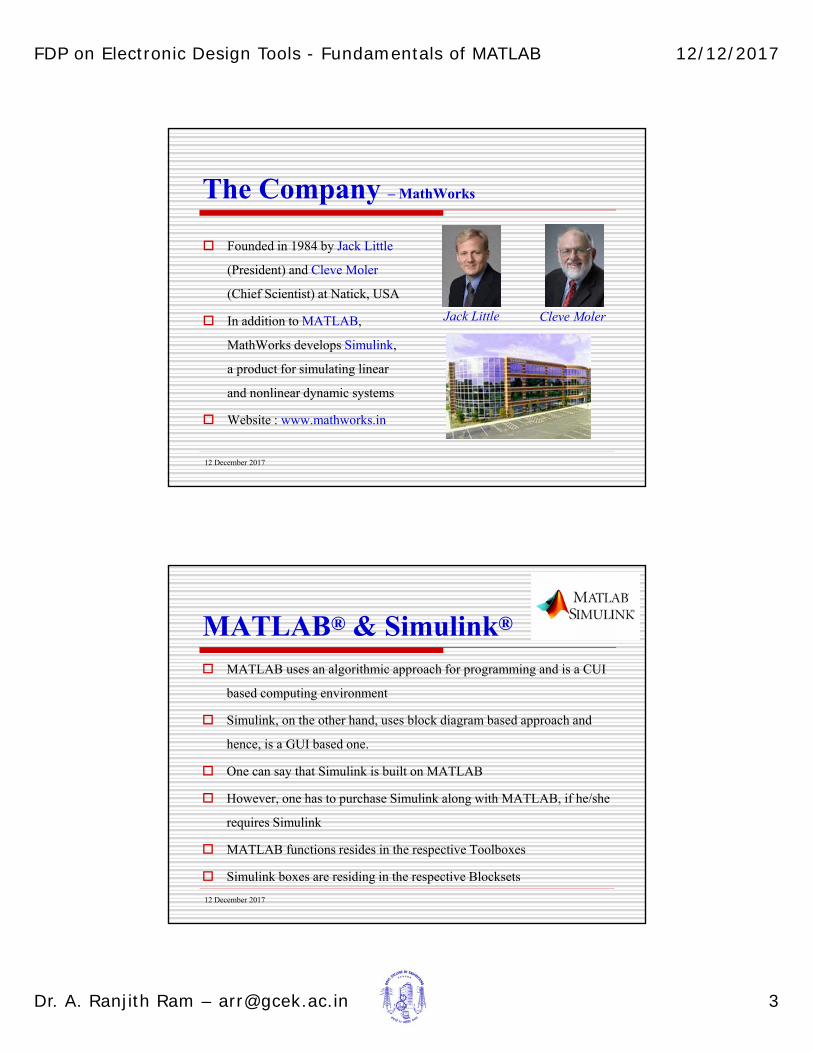
The Company – MathWorks

Founded in 1984 by Jack Little

(President) and Cleve Moler

(Chief Scientist) at Natick, USA

In addition to MATLAB,

MathWorks develops Simulink,

a product for simulating linear

and nonlinear dynamic systems

Website : www.mathworks.in

12 December 2017

Jack Little Cleve Moler

MATLAB® & Simulink®

MATLAB uses an algorithmic approach for programming and is a CUI

based computing environment

Simulink, on the other hand, uses block diagram based approach and

hence, is a GUI based one.

One can say that Simulink is built on MATLAB

However, one has to purchase Simulink along with MATLAB, if he/she

requires Simulink

MATLAB functions resides in the respective Toolboxes

Simulink boxes are residing in the respective Blocksets

12 December 2017



Where we fit MATLAB ?

Machine Language

High Level Languages such asPascal, C, C++ etc.

MATLAB

Assembly Language

12 December 2017

Features of MATLAB

MATLAB treats every data as a matrix !

MATLAB is an interpreted language, not a compiler based one

MATLAB does not need any variable declarations

MATLAB does not require any dimension statements

MATLAB has no packaging

MATLAB does not need any storage allocation

MATLAB does not require any pointers

MATLAB programs can be run step by step, with full access to all

variables, functions etc.

12 December 2017



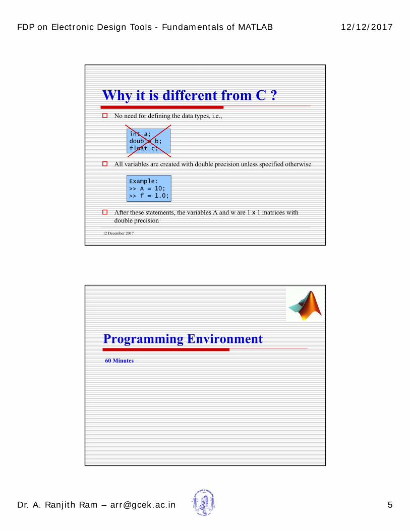
Why it is different from C ? No need for defining the data types, i.e.,

All variables are created with double precision unless specified otherwise

After these statements, the variables A and w are 1 x 1 matrices with double precision

12 December 2017

int a;double b;float c;

Example:>> A = 10;>> f = 1.0;

Programming Environment

60 Minutes



How to Open

Double Clicking the emblem

12 December 2017

Version

Product

Company

MATLAB Desktop

12 December 2017

Current Folder

Command Window

Workspace

Command History



MATLAB Desktop – Ready or Not Ready ?

12 December 2017

Ready

Not Ready !

Using the Command Window A = 10

f = 1.0;

Putting a semicolon will suppress

the output in the command window

b = (pi/180) * theta

theta should be defined !

name = ‘Sachin’ ;

character array (string)

c = f < 1 ;

logical variable

12 December 2017

If there is not an assignment, MATLAB

will automatically assign the value to a

default ans variable !

Assignment



Using Command Window (Contd…)

Clearing commands

clc ;

→ clears the

command window

clear ;

→ clears the

workspace

Use the up-arrow

(↑) for fetching the

previous command

12 December 2017

Preferences

Creating a Row Vector

r = [1 0 3 2] or [1, 0, 3, 2]

Delimiter is a space or comma

Enclosed in square braces

MATLAB takes the above as

r = [ 1 0 3 2 ]

n = [1:10] or 1:10


n = [ 1 2 3 4 5 6 7 8 9 10 ]

k = [3:2:15] or 3:2:15


k = [ 3 5 7 9 11 13 15 ]

12 December 2017



Creating a Row Vector – linspace

Suppose we want N number of data points in the interval (x1, x2)

The previous method fails here as one has to compute the step size explicitly, and one is advised to use linspace function here.

linspace – linearly spaced vector – take care of this situation in MATLAB

linspace(X1, X2) generates a row vector of 100 linearly equally spaced points between X1 and X2.

linspace(X1, X2, N) generates N points between X1 andX2.

For N = 1, linspace returns X2

linspace is useful in many signal processing and plotting situations.

linspace(1,10,13);

12 December 2017

Creating a Column Vector

12 December 2017

c = [1; 0; 3; 2]

Delimiter is a semicolon



c =

Transposing operation : using ’

r = 2:3:10 ;

c = r’ ;

1

0

3

2



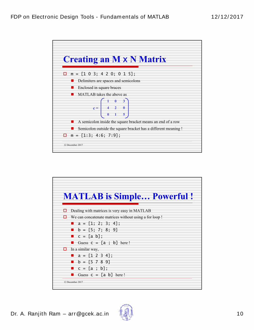
Creating an M x N Matrix

12 December 2017

m = [1 0 3; 4 2 0; 0 1 5];

Delimiters are spaces and semicolons



c =

A semicolon inside the square bracket means an end of a row

Semicolon outside the square bracket has a different meaning !

m = [1:3; 4:6; 7:9];

1 0 3

4 2 0

0 1 5

MATLAB is Simple… Powerful !

12 December 2017

Dealing with matrices is very easy in MATLAB

We can concatenate matrices without using a for loop !

a = [1; 2; 3; 4];

b = [5; 7; 8; 9]

c = [a b];

Guess c = [a ; b] here !

In a similar way,

a = [1 2 3 4];

b = [5 7 8 9]

c = [a ; b];

Guess c = [a b] here !



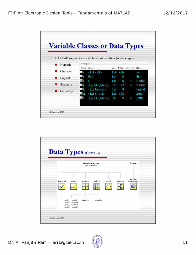
Variable Classes or Data Types

MATLAB supports several classes of variables (or data types)

Numeric

Character

Logical

Structure

Cell array

12 December 2017

Data Types (Contd…)

12 December 2017



MATLAB Toolboxes Aerospace Toolbox

Bioinformatics Toolbox

Communications System Toolbox

Computer Vision System Toolbox

Control System Toolbox

Curve Fitting Toolbox

Data Acquisition Toolbox

Database Toolbox

DSP System Toolbox

Econometrics Toolbox

Financial Toolbox

Fuzzy Logic Toolbox

Image Acquisition Toolbox12 December 2017

Image Processing Toolbox

Instrument Control Toolbox

Mapping Toolbox

Model Predictive Control Toolbox

Model-Based Calibration Toolbox

Neural Network Toolbox

Optimization Toolbox

Parallel Computing Toolbox

Partial Differential Equation Toolbox

Phased Array System Toolbox

RF Toolbox

Robust Control Toolbox

Signal Processing Toolbox

Some Built-in Functions sin()

cos()

inv()

eye()

rand()

ones()

zeros()

size()

length()

max()

min()

fliplr()

flipud()

12 December 2017

plot()

stem()

surf()

mesh()

fft()

abs()

eig()

rank()

ceil()

round()

sum()

prod()

linspace()



Help / Documentation

help function_name

Help Menu

Search

12 December 2017

or doc function_name

Tea Break !

10 Minutes



Matrix Algebra

40 Minutes

Matrix Addition & Subtraction Matrix addition : +

a = [1 2 3 4];

b = [5 6 7 8];

c = a + b

yields c = [6 8 10 12]

Matrix subtraction : –

a = [7 2 6 9];

b = [5 6 7 8];

c = a - b

yields c = [2 -4 -1 1]

Both the matrices should be of the same dimensions.

Equivalent to addition and subtraction of two signals

12 December 2017



Matrix Multiplication Matrix multiplication : *

a = [1 2 3 4; 3 1 2 4];

b = [3 1; 1 2; 0 1; 2 3];

c = a * b

yields c = [ 13 20

18 19 ]

Both a & b should be conformable to multiplication

a should be of dimension M x N and b should be of N x K

The result will be of M x K dimension

Multiplication by a scalar is also done using *

The function equivalent to * is mtimes()

c = mtimes(a, b)

12 December 2017

Signal Product Signal multiplication is done using .*

.* will compute the element-by-element product

a = 1:5;

b = 2:6;

c = a .* b

will yield c = [ 2 6 12 20 30 ]

Matrix dimensions must match.

Will output a signal of same dimension

Is useful is many signal processing operations

The function equivalent to .* is times()

Check:

pow = a .* a; and pow = a .^ 2;

12 December 2017



Matrix Division (?)1. Matrix division using /

a = [1 2 3; 0 1 2; 3 0 4];

b = [3 0 1; 1 2 0; 0 1 3];

c = a / b

yields c = [0.1579 0.5263 0.9474

-0.0526 0.1579 0.6842

1.1579 -0.4737 0.9474]

a / b computes a * inv(b)

2. Matrix division using \

a \ b computes inv(a) * b

Find the inverse of a using \

a \ eye(size(a))

12 December 2017

Matrix Indexing and Addressing

In MATLAB, the indexing is from 1 to N, unlike from 0 to N–1 in DSP theory or C Language

This practicality is to be taken care of when the an algorithm in theoretical DSP is getting implemented using MATLAB

normal braces ( ) are used for addressing elements of a matrix

temp(5,10) selects the element in the 5th row and 10th column of the matrix temp

marks(:,3) selects the third column of the matrix marks

marks(2,:) selects the second raw of the matrix marks

lena(:,:,2) selects the green component of the colour image lena

face(20:50,30:60,:) will select a rectangular region of the colour image face

12 December 2017



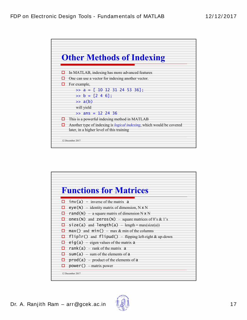
Other Methods of Indexing

In MATLAB, indexing has more advanced features

One can use a vector for indexing another vector.

For example,

>> a = [ 10 12 31 24 53 36];

>> b = [2 4 6];

>> a(b)

will yield

>> ans = 12 24 36

This is a powerful indexing method in MATLAB

Another type of indexing is logical indexing, which would be covered later, in a higher level of this training

12 December 2017

Functions for Matrices inv(a) – inverse of the matrix a

eye(N) – identity matrix of dimension, N x N

rand(N) – a square matrix of dimension N x N

ones(N) and zeros(N) – square matrices of 0’s & 1’s

size(a) and length(a) – length = max(size(a))

max() and min() – max & min of the columns

fliplr() and flipud() – flipping left-right & up-down

eig(a) – eigen values of the matrix a

rank(a) – rank of the matrix a

sum(a) – sum of the elements of a

prod(a) – product of the elements of a

power() – matrix power

12 December 2017



Methods of Data Input & Output

10 Minutes

Data Input

Generally there are three ways of inputting data into MATLAB

directly entering in the command line

from memory

read an excel file

read a speech file

read an image file

from I/O devices

input from a sensor

input from a microphone

input from a camera

12 December 2017



Data Input – Examples

fc = input('Enter the carrier frequency: ');

x = xlsread(‘table.xlsx');

wavread(‘aud.wav’);

imread(‘lena.jpg’);

S=load(‘filemname’);

import menu – import a file

12 December 2017

Data Output

Generally there are three ways of outputting data from MATLAB

directly flashing to command line

to memory

write an excel file

write a speech file

write an image file

to I/O devices

output to a DAC

output to a loudspeaker

output to a display

12 December 2017



Data Output – Examples

sprintf(‘The bandwidth is %d', bw) or display(bw)

fid = fopen('exp.txt','w');

fprintf(fid,'%6.2f %12.8f\n',y);

fclose(fid);

xlswrite(‘t.xlsx’,m)

wavwrite(s,fs,‘au.wav’)

imwrite(y,‘img.jpg’)

save(‘filename’, var)

save menu12 December 2017

/ sound(s,fs)

/ imshow(y)

Reserved Characters / Words

10 Minutes



Characters and Meaning ; suppressing output in the command window

= assignment

+ addition

- subtraction

* matrix product

/ post multiply with inverse

\ pre multiply with inverse

< less than

> greater than

~ logical not

& logical and

| logical or

12 December 2017

Characters and Meaning (Contd…)

. element wise operation, decimal point, structure field access

.. parent directory

… continuation

: range

[ ] matrix entry

( ) addressing array elements, function

{ } cell array addressing

% commenting

^ power

‘ ’ string entity

’ complex conjugate transpose

@ function handle

12 December 2017



Reserved Characters / Words

i imaginary notation

j –do–

pi 3.14…..

Inf infinity

NaN not a number

eps spacing of floating point numbers

who prints variables in work space

why answers to such a question. Do chat with MATLAB !

beep produces a beep sound

12 December 2017

Basic Computing and Plotting

40 Minutes



Roots of a Polynomial roots(C) computes the roots of the polynomial whose coefficients

are the elements of the vector C

If C has N+1 components, the polynomial is C(1) * X^N + ... +

C(N) * X + C(N+1).

C = [1 0 -3 2 ];

r = roots(C)

yields r = [-2 1 1]

p = poly(r) converts the roots to its polynomial

yields p = [1 0 -3 2]

12 December 2017

One Dimensional Plots plot(x, y)

plots vector y versus vector x

If x or y is a matrix, then the vector is plotted versus the rows or columns of the matrix, whichever line up

plot(y) plots the columns of y versus their index

if y is complex, plot(y) is equivalent to plot(real(y), imag(y))

in all other uses of plot, the imaginary part is ignored

stem() – plots a signal in a sampled fashion

bar() – plots a signal in bar form

stairs() – plots a signal in staircase form

scatter() – plots in the form of scatter diagram

12 December 2017



Plotting Trigonometric Functions Let the time duration of the waveform be one second i.e., 0 – 1 second

Let the amplitude be 10 and frequency be one Hertz.

t = 0 : 0.01 : 1;

f = 1; A = 10 ;

x = A*sin(2*pi*f*t);

plot(t, x);

This yields an output figure :

Use close command to close

a figure (close all : closes all figures)

12 December 2017

stem(t,x)

Ensure sufficient samples ! t = 0:0.1:1;

t = 0:0.01:1;

12 December 2017



Plotting – More features

Choosing colour and line width

Adding title, x-label & y-label, grid lines and legends

Choice of range of the independent and dependent variable axes

plot(t,x,’r’,‘LineWidth’,2);

grid on;

axis([-1 2 -15 +15])

title(‘The Sine Wave’);

xlabel(‘Time’);

ylabel(‘Amplitude’);

legend(‘Sin(2pift)’)

12 December 2017

Am

plitu

de\pi

Multiple Plots in a Window Using subplot() function

subplot initializes a tiled space in a figure window

After subplot,

a plot function

is to be used for

actual plotting

12 December 2017

subplot(221) subplot(222)

subplot(223) subplot(224)



Multiple Plots in a Window (Contd…)

t = 1:200;

subplot(221)

plot(exp(-0.01*t), ’r’);

subplot(222)

plot(exp(-0.02*t), ’g’);

subplot(223)

plot(exp(-0.03*t), ’b’);

subplot(224)

plot(exp(-0.04*t), ’k’);

12 December 2017

Plots in Different Windows

figure(1)

plot(exp(-0.01*t), ’r’);

figure(2)

plot(exp(-0.02*t), ’g’);

figure(3)

plot(exp(-0.03*t), ’b’);

figure(4)

plot(exp(-0.04*t), ’k’);

12 December 2017



Plots on the Same Axes plot(exp(-0.01*t), ’r’);

hold on;

plot(exp(-0.02*t), ’g’);

hold on;

plot(exp(-0.03*t), ’b’);

hold on;

plot(exp(-0.04*t), ’k’);

legend(‘e^{-0.01t}’,‘e^{-0.02t}’,‘e^{-0.03t}’, ...

‘e^{-0.04t}’)

hold off;

12 December 2017

M-Files / Script Files

10 Minutes



When to Create a Script File t = 0:0.01:1;

f = 1.0;

x = 10*cos(2*pi*f*t);

plot(t, x, ’r’);

title(‘The Sine Wave’);

xlabel(‘Sampling Instants’);

ylabel(‘Amplitude’);

If one has to find/plot a function after changing the value of one of the variable, he/she has to execute all the subsequent commands one by one

At this point, script files or m-files need to be created

It is created using an editor which is having all the features like cut/copy-paste, undo, indent, insert, save as, etc.

12 December 2017

Command line based computation has its own limitations

Creating a Script File Click on the New Script menu on the MATLAB Desktop

12 December 2017



Developing a script file Enter all the instructions line-by-line in the editor

Or, Select the group of commands from the command history and right-click on the selection to create script

12 December 2017

Running a Script File Click on the Run Button on the Editor Menu

12 December 2017



Few Points on Script Files

A script is to be saved before running it (for the first time)

MATLAB saves the script is the current directory by default

If the user saves the script in another folder, MATLAB will ask for the options of ‘Change Folder’ or ‘Set Path’ while running

Opt ‘Change Folder’. Then you will be using MATLAB from your folder

Care should be given on aming the script file :

The filename should always start with an alphabet !

The filename should not be the same as any of the built-in functions !

Spaces can not appear in between !

One can use underscore (_) or hyphen (– ) to connect words

Adopt your own policy when naming script files. It may be better to reflect the purpose for which the program is developed.

12 December 2017

Exercises

1) Plot the function x(t) = e–at

2) Plot the function x(t) = 1 – e –at

3) Plot the function x(t) = 6 Sin(at) 4 Cos(bt)

4) Plot the function x(t) = Cos(bt) e–at

5) Plot the function f(x) = sinc(x)

6) Plot the function f(x) = (1/√2πσ) e– (x – μ)2 / 2σ2

7) Plot the function x(n) = e–an

8) Plot the function x(n) = 6 Sin(an) 4 Cos(bn)

12 December 2017



Part – I : Summary

Familiarized with MATLAB desktop, toolboxes, variable classes and some built-in functions

Performed simple computations using the command prompt, reviewed fundamentals of linear algebra using MATLAB

Differentiated the matrix product from signal product

Studied how to seek help in the command prompt and how to use the help menu

Learnt the various methods of data input and output

Computed the roots of a polynomial and obtained the polynomial from a root set

Learnt how to plot one dimensional (1-D) curves

Studied how to create and run the MATLAB script files

12 December 2017

12 December 2017

Thanks

Courtesy :

1. MathWorks Training & Services, Bengaluru

2. TEQIP Project Phase-II, GCE Kannur

[email protected] : 09447637667

FDP on Electronic Design Tools - Fundamentals of...

Documents

Transcript of FDP on Electronic Design Tools - Fundamentals of...