FDM 13-25 Storm Sewer Design - Wisconsin Department of ...wisconsindot.gov/rdwy/fdm/fd-13-25.pdf ·...

Facilities Development Manual Wisconsin Department of Transportation Chapter 13 Drainage Section 25 Storm Sewer Design

FDM 13-25-1 Introduction August 8, 1997

1.1 Introduction

For the design of an underground storm drain system, it is necessary to have complete and accurate information regarding the existing system. If the existing system is to be used it should be carefully checked hydraulically and physically to show it is adequate to accommodate the additional water from the highway improvement. If possible, a check of the energy losses associated with the system should be performed (refer to Pressure Flow, FDM 13-25-35).

On new projects where the existing sewer is a combination storm and sanitary system, every effort should be made to remedy the situation by separating the sewers.

Storm sewers shall not alter the existing drainage pattern, and the sewer outfalls shall be located at existing drainage ditches and/or natural low points.

The latter steps in the design of the storm sewer may require the designer to go back and change initial assumptions.

If catch basins are installed on a project, a maintenance schedule should be developed (refer to FDM Chapter 10).

Attachment 1.1 shows a flowchart that describes the various steps of a storm sewer design.

LIST OF ATTACHMENTS

Attachment 1.1 Storm Sewer Design Flow Chart

FDM 13-25-5 Basic Drainage Area Information August 8, 1997

5.1 Basic Information Needs

Before the design engineer commences designing a storm sewer system, the following basic information should be collected on the specific area to be drained by the proposed system:

1. Aerial photographs showing the existing land use patterns.

2. A contour map of the area where the storm sewer is to be built. Use a scale of 1" = 100' (1:1200) or 1"= 50' (1:600) with a two foot contour interval.

3. A U.S.G.S. map (scale 1" = 2,000' or 1" = 5,208'), (1:24000 or 1:62500) of the drainage basin containing the area being studied.

4. Soil maps for aid in estimating the runoff potential.

5. Water table data from available borings or maps.

6. A layout of the area where the storm sewer is to be built. This should show the existing or proposed streets, intersections, and development type.

7. Plans of any existing drainage system.

8. Typical street cross section.

9. Street and intersection grades of the area under study.

10. Information on existing and proposed underground utilities.

11. Location, ground elevation, and high-water records for the outfall point of the proposed storm sewer system and/or the existing storm sewer system.

12. Rainfall curves appropriate to the drainage area. Refer to FDM 13-10-5.

13. Local design standards, land use information, and future drainage plans obtained from the appropriate local governmental unit.

http://wisconsindot.gov/rdwy/fdm/fd-10-00toc.pdf#fd10

http://wisconsindot.gov/rdwy/fdm/fd-13-25-att.pdf#fd13-25a1.1


http://wisconsindot.gov/rdwy/fdm/fd-13-10.pdf#fd13-10-5


FDM 13-25 Storm Sewer Design

14. Field inspection data from the area under study.

15. Locations of sensitive areas and any potential source of pollutants. Refer to Chapter 10.

FDM 13-25-10 Field Drainage Information August 8, 1997

10.1 Field Information Needs

Field information must be collected for the drainage area to be served by a storm sewer in order to update the existing land use patterns and to verify the direction of overland flow in the vicinity of the highway. In this field review, the following steps should be taken:

1. Field-walk the drainage area, taking note of any natural waterways, ditches, sinkholes, dry wells, ponds, tiles, or anything else affecting drainage not previously recorded.

2. Record the location of any existing and/or possible outfalls. This will facilitate the mapping of possible drainage easements.

3. Record the location and depth of underground utilities not shown on any maps (water, gas, electric, telephone, sanitary sewers, storm sewers, etc.).

4. Verify the office-estimated runoff coefficients through field-checking the topography of the drainage area.

5. Check with local residents, local maintenance foremen, and municipal officials, etc., for any possible problem areas, such as flooding of lowlands.

6. Identify and locate sensitive areas and any potential source of pollutants. (refer to Chapter 10).

FDM 13-25-15 Preliminary Layout of System November 26, 1997

15.1 Background Information

The preliminary layout of a storm sewer system is divisible into two major operations as follows:

1. Locate and space inlets.

2. Prepare a plan layout of the storm sewer system showing the following data:

- Location of all underground utilities in the plan and profile. Also plot these utilities on cross sections.

- Location of the main storm sewer line.

- Direction of flow.

- Location of inlets.

- Location of manholes.

- Location of outfall(s).

- Shape and type of conduit.

The preliminary plan can be constructed through the application of the design criteria that follow.

15.2 Inlet Locations

Maximum Spacing: Water should normally not travel more than 300 to 600 feet before interception, with the closer spacing employed for flat terrain and for high-speed highways. Moreover, spacing of inlets should be designed to prevent water from spreading over more than one-half of the traveled lane and from overtopping the curb. Since a parking lane or shoulder is not considered a traveled lane, the flow of water can utilize the full parking lane or shoulder width. However, the future expansion of the roadway should be considered before the full parking lane is used for conveyance of water.

At Low Points: In a curb section, at least one inlet must be located at the low point of each sag vertical. However, if there is a possibility of clogging because of high quantities of debris, two inlets should be installed - one at the low point and one where the grade elevation is about 0.20 foot higher than at the low point. Hydraulic Engineering Circular No. 12 “Drainage of Highway Pavements” has a discussion about the use of flanking inlets.

At Bridge Ends: Generally, inlets should be placed to intercept the gutter flow before it reaches the bridge.

At Intersections: Inlets at intersections are to be placed in order to intercept the gutter flow before it reaches a pedestrian crosswalk.




Prevention of Cross Pavement Flow: The flowing of water across pavements should be prevented in order to preclude icing in the winter and hydroplaning during the warmer months. In particular, where pavements are super-elevated, inlets shall be placed to intercept the gutter flow before the pavement becomes too flat for effective pickup.

Driveway Openings: Where driveways have a descending grade from the gutter, the installation of inlets might be necessary to preclude the design storm from overflowing at the driveway openings. However, to minimize the number of inlets, the driveway cross section should be designed with a gutter sufficiently deep to accommodate the design flow.

Side Drainage: Drainage from outlying areas should be intercepted before it reaches the roadway pavement, especially where mud and debris will be carried onto the pavement.

15.3 Conduit Location

The location or lateral placement of a conduit system is dictated by economics, hydraulic requirements, ease of construction and maintenance, and local community preference.

Proposed storm sewer shall be laid at least 8 feet horizontally from any existing or proposed water mains. The distance shall be measured from center to center. In cases where it is not practical to maintain an 8 foot separation, Chapter NR 811 of the Wisconsin Administrative Code shall be consulted for additional guidelines.

Curvilinear and angular alignments in conduits produce hydraulic losses. Therefore, if possible, any change in alignment between structures is to be avoided, especially on trunk or main line segments of a storm sewer system. For pipes with diameters of 30 inches or more, a long radius curve of 100 feet or more is permissible. The radius of curvature specified shall be one of the available standard manufactured curves in the specified type of material.

On lateral lines, an angular change in alignment for conduit of 30 inches or less in diameter is permitted.

15.4 Standards for Storm Drain Pipe

Pipe Diameter: The minimum pipe diameter shall be as follows:

Type of Drain Minimum Diameter (Inches)

Trunk Line

Trunk Laterals

Inlet Laterals

[1]24"

15"

12"

[1] For short runs, smaller sizes may be specified.

Under special conditions, such as a problem with fine debris or flat grades, the minimum pipe size for laterals should be 18 inches

Pipe Strength: Strength requirements for pipe shall conform to the ASTM designations for the type and class of pipe as given in the approved practice drawing.

Pipe Slope: Refer to FDM 13-25-35, for minimum pipe slopes.

15.5 Manholes

Purpose: The principal purpose of a manhole is to provide maintenance access to a continuous underground conduit.

Types: Refer to Chapter 16 of this manual for standard detail drawings of approved manholes. Special manholes shall be designed when conditions make the use of the above-listed manholes not feasible. When a manhole is used as an inlet, the design criteria for inlets apply.

Location: In general, manholes are to be located as follows:

1. At the end of existing and future lines

2. Where the conduit changes size

3. At sharp curves or angles in the line (10° or over)

4. At points where there is an abrupt change in grade

5. At all intersections



6. At junctions of sewers

If possible, avoid locating manholes in traffic lanes. When manholes must be placed in traffic lanes, care shall be taken to avoid the normal wheel tracks.

Spacing: To facilitate maintenance operations, manhole spacing should be as follows:

Size of Pipe in Inches Maximum Distance in Feet

12 through 24

27 through 36

42 through 54

60 or larger

350

400

500

1,000

In cases where a municipality has its own policy on spacing of manholes, requiring a lesser maximum spacing, consideration may be given to that policy.

15.6 Outfalls

To preclude an expensive design, care should be taken to avoid placing an outfall underwater or where water might back up into the system. In general, sewer outfalls shall be placed at existing drainage ditches and natural low points.

FDM 13-25-20 Design Discharge August 8, 1997

20.1 Design Discharge Information

The design discharge used in sizing storm sewer systems should be determined by the Rational Formula. Refer to FDM 13-10-5 for a thorough explanation of the theory and application of the Rational Formula.

When side drainage is collected in the system, the peak discharge must be estimated for the following two separate conditions:

1. Fast runoff from short-duration, high-intensity rainfalls. These peak flows originate only from the connected impervious areas adjacent to the storm sewer, e.g., streets, sidewalks, parking lots, etc.

2. Slow runoff from long-duration, low-intensity rainfalls. These peak flows originate from the total area draining toward the storm sewer.

Since storm sewers are sized for the largest peak flow produced by a specific design frequency, the controlling condition is the one that produces the largest peak flow.

For urban streets, the rainfall intensity should be determined on a 10-year (check 25-year) frequency with a rainfall duration equal to the minimum time of concentration or five minutes, whichever is greater. If the check using the 25-year storm results in unacceptable conditions (highway inundation, flooding, etc.), the sewer shall be sized accordingly to alleviate the effects of backwater associated with the proposed sewer system (refer to FDM 13-25-45 for a design using surcharged full flow).

In cases where the municipality has its own criteria for the design of a sewer system, consideration may be given to those criteria.

Intensity for interstate and freeway projects shall be determined for a minimum time of concentration of five minutes on a 25-year frequency. At sag points, such as roadway underpasses a check of the Hydraulic Gradeline (HGL) should be made using the 50-year storm.

A weighted or composite runoff coefficient shall be determined as explained in FDM 13-10-5.

FDM 13-25-25 Gutter Design August 8, 1997

25.1 Capacity

The hydraulic design of gutters consists of determining the spacing of inlets to avoid the undue spreading of water over the pavement, or determining the height of water at the face of curb if the spacing is predetermined. The gutter capacity is determined using Attachment 25.1, which applies to triangular channels and other shapes shown in the figure.





25.2 Gutter Types

Refer to FDM 16-5-1 for standard detail drawings of approved curb and gutter cross sections.

25.3 Longitudinal Slopes

Preferable minimum longitudinal gutter grades shall be 0.5 percent, with an absolute minimum of 0.3 percent, except in short runs that will carry no appreciable flow.

Example Problem

Given:

1. Type A Curb and Gutter, 30-Inch.

2. Longitudinal Pavement Slope = 1.0%.

3. Crown of Pavement = 2.0%.

4. Street Width Face-to-Face = 28 feet.

Find:

1. The maximum allowable flow Qp for the above type of street section.

Solution:

See Attachment 25.2 for a sketch of the street cross section. The process involves the following steps.

1. Determine the maximum allowable flow in combined areas "b" and "c," Q(b+c).

1.1 From FDM 13-25-15, up to one-half of the traveled lane width may be used to convey storm water flow as long as the curb is not overtopped. In this case half the traveled lane width is 6 feet.

1.2 The maximum depth, d', in area (b+c) is d' = 6 feet x 0.02 or 0.12 feet.

1.3 Use Attachment 25.1 and the data below to calculate Q(b+c).

- S= 0.01 ft/ft (given)

- Z(b+c) = 1/.02 = 50 (defined in Attachment 25.1)

- n= .015 (from Attachment 35.1)

- Z(b+c) /n = 3333

- From the nomograph in Attachment 25.1: Q(b+c) = 0.65 cfs

2. Determine the maximum allowable flow in combined areas "a" and "c," Q(a+c).

- From SDD 8d1, the cross slope of Type A curb & gutter is 3/4 inch per ft or 0.0625 ft/ft and the gutter width is 2 ft.

- The depth, d, at the curb is d' + (2 ft x 0.0625 ft/ft) or 0.245 ft. Note the curb is not overtopped so the flow is allowed to extend to half the width of the traveled lane.

- Other data:

The values for "S" and "n" remain the same as in Step 1 above.

Z(a+c) = 1/.0625 = 16

Z(a+c) /n = 1067

Again, using the nomograph and solving for discharge, Q(a+c) = 1.5 cfs

3. Determine the maximum allowable flow for area "c," Qc.

- The values for "S," "n" and cross slope remain the same as in Step 2 above so the value for Zc/n is the same as Z(a+c)/n above.

- The maximum depth is d' or 0.12 ft.

- From the nomograph, Qc = 0.25 cfs

4. Determine total maximum allowable flow.

Qp = Q(b+c) + Q(a+c) - Qc

Qp = 0.65 + 1.5 - 0.25 = 1.90 cfs

In this situation, an inlet must be provided before the volume of flow reaches 1.90 cfs in order to prevent the







http://wisconsindot.gov/rdwy/sdd/sd-08d01.pdf#sd8d1


storm water from infringing too far into the traveled lane.

LIST OF ATTACHMENTS

Attachment 25.1 Gutter Design Nomograph

Attachment 25.2 Gutter Design Example

FDM 13-25-30 Hydraulic Design of Inlets August 8, 1997

30.1 Inlet Types

A storm water inlet is a means of admitting storm water into a storm sewer system. Inlets are either constructed on a continuous grade or in a sump condition, and the gutter is either depressed or not depressed. The term "continuous grade" means that the grade of the street is continuous past the inlet. The sump condition exists whenever the water is restricted to the inlet because the inlet is in a low point. The five general types of inlets along with some general information on their use and several examples are listed below. For more thorough discussion, it is recommended that designers obtain a copy of FHWA's Hydraulic Engineering Circular (HEC) #12, Drainage of Highway Pavements. A copy can be obtained for a fee by contacting National Technical Information Services at 1-800-553-6847 and asking for publication FHWA-TS-84-202. Manufacturers, such as Neenah Foundry, should also be contacted when special designs are being considered.

30.1.1 Curb Opening Inlets

A curb opening inlet consists of a vertical opening in the curb through which the gutter flow passes. The major advantage of the curb opening inlet is that it does not clog easily through trapping of debris; instead, the debris readily passes through the curb opening into the storm sewer system.

The capacity of this inlet is increased significantly by depressing the gutter. They perform well where orifice flow may occur, such as in sag or flat conditions. On continuous grades they do not perform well because gutter flow typically bypasses the opening.

30.1.2 Grated Inlets

Basically, a grated inlet consists of an opening in the gutter covered with a grate. The bars may be oriented either longitudinally or transverse to the flow. Although longitudinal grates are more efficient than transverse grates, longitudinal grates are not permitted where bicycle traffic is permitted. However, the efficiency of transverse grates has been improved by designing the bars as vanes slanted at 55 F from the horizontal plane (refer to Chapter 16 for standard detail drawings of these special grates). These grates must be oriented with the slant in the direction of the oncoming flow. Improperly installing the grate will result in virtually 100 percent overflow.

The major disadvantage of grated inlets is that they tend to plug, especially in a sump condition.

Depressing of gutter will significantly increase its capacity; because there is no curb opening to handle possible clogging of the grate, this depression may be undesirable from a traffic standpoint.

30.1.3 Combination Inlets

A combination inlet is composed of both a curb opening inlet and a grated inlet, with the grated inlet usually placed directly in front of the curb opening. In sump conditions, grated inlets in combination with curb openings are advisable since the grate is more apt to plug.

Curb openings on a continuous grade do not efficiently trap water and may not be the best alternative in areas where water quality is a concern. Using curb openings with grates on a continuous grade may be useful in situations where debris is a problem. If debris clogs the grate the curb opening will still handle a minimal amount of the gutter flow.

One alternative to using curb openings is to evaluate grates that have been designed for debris handling efficiency. This information can be best obtained by contacting inlet manufacturers.

Capacity of a combination inlet on grade with a curb opening can be improved if a "sweeper inlet" is used. A sweeper inlet is a combination inlet that has the curb opening upstream of the grate so as to intercept debris and capture some of the gutter flow prior to it entering the grate. Designers should follow H.E.C. #12 for guidance on calculating the inlet capacity of sweeper inlet.

Theoretically, in a sump condition the combination inlet exhibits a high flow capacity; however, this is questionable because of the grate plugging, thus leaving only the curb opening to handle the gutter flow.





In sump conditions, combination inlets are considered advisable where ponding can occur. When in weir flow, the interception capacity of the combination inlet is essentially equal to that of a grate inlet alone, unless the grate becomes clogged. In orifice flow, the capacity is equal to the capacity of the grate plus the capacity of the curb opening (see H.E.C. #12 for examples). Flanking inlets are recommended where significant ponding can occur, such as underpasses and sag vertical curves in depressed conditions.

30.1.4 Multiple Inlets

A multiple inlet consists of two or more closely spaced inlets acting as a unit. The inlets may be any combination of the above-explained types. The characteristics of a specific multiple inlet are the same as the characteristics of each individual inlet type used to construct the multiple inlet. Care should be taken to avoid placement in traffic lanes and interference with bicycle traffic.

Grate inlets are often placed next to each other for this purpose. They perform best when in parallel and adjacent to each other as opposed to adjacent in series along the gutter. However, should placement in series be preferred, inlets should be spaced apart from each other at a distance that allows the bypass flow to return the curb face. If this is not done, the second grate will not provide the capacity it was designed for as most of the water will bypass it.

When inlets are placed in a series, the recommended minimum spacing (a function of the discharge, longitudinal slope, and transverse slope) should be from six to 20 feet to allow the bypass flow to return to the curb face.

30.1.5 Slotted CMP Surface Drains

This type of inlet consists of a corrugated metal pipe with a continuous slot on top. The slot is formed by a pair of angle irons, which serves as a paving bulkhead. They can be used on curbed or uncurbed sections and offer little interference to traffic operations. See discussion and examples presented in this procedure and HEC #12.

30.2 Allowable Inlet Capacities

The allowable inlet capacity is computed as a percentage of the theoretically calculated capacity. This compensates for the decreased capacity of the inlet through debris clogging, pavement overlapping, varying design assumptions, etc. The allowable design capacity for an inlet is determined by applying the reduction factors from Attachment 30.1 to the theoretical capacity calculated by the design process described in this procedure.

Though application of these reduction factors may be needed in a sump or relatively flat condition to account for potential clogging, they may not be needed for inlets on continuous grade. Partial clogging rarely causes major problems for inlets on grade. Therefore, reduction factors should be applied to inlets on grade only "when local experience indicates an allowance is advisable." To help determine whether a reduction factor is needed, designers should do a site investigation and inquire with maintenance staff, and those familiar with the area, to evaluate whether clogging is a problem.

30.3 Capacities of Grate Inlets and Combination Inlets on a Continuous Grade

The capacity of both grate inlets and combination inlets depends on both the length and the depression of the inlet, the depth of flow in the gutter at the curb line, and both the cross slope and the longitudinal slope of the gutter.

The general equation used to determine the capacity of a grate inlet is:

Q = KD5/3

Where:

Q = grate inlet capacity in cfs.

K = an empirical coefficient for a specific grate, with the appropriate design longitudinal and transverse slopes.

D = curb line flow depth (in feet) upstream from the grate

The Neenah Foundry Company has developed for each grate that they manufacture a chart that gives values of K versus transverse slope ST (0 to 0.06 ft./ft.)

For longitudinal slopes SL of one, two, four, and six percent. Charts for most WisDOT-approved grate types may be obtained from a Neenah Foundry publication entitled "Neenah Inlet Grate Capacities" (1).

For unusual situations, such as a depressed inlet, etc., the designer is referred to the research work of John



Hopkins University (2).

Example Problem

Capacity of a Combination Inlet Grate on a Continuous Grade

Given: Type A Curb and Gutter, 30-Inch

Longitudinal Slope SL = 1.0% Crown of Pavement = 2.0% Transverse Slope of Gutter ST = 0.0625 ft./ft. Street Width Face-to-Face = 28 feet Inlet Type H

Find: The allowable inlet capacity for the above design criteria when the gutter is flowing at the allowable capacity.

Solution:

1. Design equation is Q = KD5/3.

2. From the example problem of FDM 13-25-25:

Allowable D = .245 foot

3. From Neenah Inlet Grate Capacities Manual(1) with ST = 0.0625 ft./ft., SL =1%:

K = 12.5 for a Type H inlet (extrapolated)

4. Therefore, without clogging, the Type H inlet grate capacity is:

Q = KD5/3

Q = 12.5 (0.245) 5/3

Q = 1.20 cfs

5. From Attachment 30.1, the reduction factor R.F. for a combination grate on a continuous grade is:

R.F. = 1.10 x .50 = .55

6. Therefore, the allowable inlet capacity is:

Q(all.)= .55 x 1.20 cfs = .66 cfs

30.4 Capacity of Grate Inlets in a Sag

Depending upon the depth of flow, grate inlets operate under three different conditions of flow:

1. Weir flow (flow depth less than 0.4 foot)

2. Transitional flow, undefinable flow because of vortices and other disturbances (flow depth from 0.4 and 1.4 feet); or

3. Orifice flow (flow depth greater than 1.4 feet).

For transitional flow, the grate inlet capacity is somewhere between the inflows predicted by the weir and orifice flow equations.

The capacity of grate inlets in a sag condition may be determined with the aid of the FHWA H.E.C. #12 publication entitled "Drainage of Highway Pavements" (3).

Specifically, Chart 11 of H.E.C. #12 may be used to graphically solve for a weir or orifice flow condition.

In order to use this chart, the designer must know the effective perimeter and/or inflow area of the selected grate. The effective perimeter may be easily computed from the grate dimensions, while the inflow area may be obtained from a Neenah Foundry publication entitled "Neenah Inlet Grate Capacities" (1).

In addition, the Neenah Foundry publication also contains a nomograph for easy solution of only the orifice flow condition.

30.5 Capacity of Curb Openings in a Sag

As with grate inlets, curb openings operate under three different conditions of flow:

1. Weir flow depth less than the height (h) of the curb opening;

2. transitional flow, undefinable flow because of vortices and other disturbances (flow depth from h and



1.4 h); or

3. orifice flow (flow depth greater than 1.4 h).

Although not empirically correct, for the sake of a design solution it is suggested that designs in the transitional zone be accomplished with the orifice equation. The FHWA publication H.E.C. #12 (3,) contains a thorough discussion along with an example problem for determining the capacity of curb openings in a sag.

30.6 Spacing of Inlets on a Continuous Grade

The spacing of inlets is determined by:

1. The design discharge,

2. the carrying capacity of the gutter, and

3. the allowable spread of water on the pavement. Moreover, the spacing of inlets by hydrologic and hydraulic computations requires a trial and error solution for streets that have varying grades, widths, and cross slopes.

The peak flow rate is determined by the Rational Equation, which is fully explained in FDM 13-10-5. Furthermore, the peak flow rate may result from participation of the entire drainage area or only the pavement surface with all the directly connecting impervious areas. Since the time of concentration in most design cases will be less than five minutes, the rainfall duration will be the standard five-minute minimum.

The economical design of inlets requires that a certain amount of bypass flow be allowed to pass to the next inlet. In certain situations, such as pedestrian crossings, the bypass flow may have to be captured by a second inlet, which should be located a minimum of six to 20 feet downstream from the first inlet. In most cases, standard highway inlets have enough capacity to catch all gutter flow within the width of the inlet.

Procedure

With only pavement runoff, the general procedure for the spacing of inlets on a continuous grade is as follows:

1. Locate the high points on the profile.

2. Estimate the average gutter grade from the high point or the last inlet location to the approximate location of the next inlet.

3. Determine the allowable gutter flow Qp using FDM 13-25-25.

4. Select a trial inlet and determine the allowable inlet capacity Qi using the design methodology explained in this procedure under the heading "Capacity of Grate Inlets and Combination Inlets on a Continuous Grade."

5. Determine the five-minute duration, 10-year frequency rainfall intensity "I" from the appropriate intensity-duration-frequency curve, FDM 13-10-5, Attachment 5.4.

6. Determine the pavement-gutter width "W" contributing runoff to the subject inlet.

7. a. First inlet only, the design discharge QD equals the allowable gutter flow: QD = Qp. Using this design flow in step 8 will give the length of street necessary to produce a gutter flow equal to the allowable gutter flow.

b. Subsequent inlets, the design discharge equals the allowable gutter flow minus the bypass flow QB from the last inlet or the allowable capacity of the present inlet Qi, whichever flow is less: QD= Qp – QB

or QD- Qi.

8. Estimate the inlet spacing L in feet by substituting the above values into the equation L = 48500 QD/IW, with QD in cfs, I in./hr., and W in feet.

9. For vertical curved sections, check the assumed grade from step 2 with the actual average grade based on the inlet location of step 8. An error in grades of + or - 10 percent indicates an acceptable solution; however, if the error is greater than + or - 10 percent, repeat procedure starting with step 2.

For curb and gutter sections that carry overland side flow as well as pavement runoff, the above procedure is not applicable. However, if the side flow area is of a uniform width parallel to the street, the above procedure, with modifications of steps 6 and 8, can be used. Step 6 should be modified so that W includes the width of the side flow area as well as the street width. The equation in step 8 has a hidden runoff coefficient of 0.9 for paved areas. With runoff also from impervious areas, this must be replaced by a composite runoff coefficient C, which produces the following equation: L = 43560 QD/IWC, with L in feet, QD in cfs, I in./hr., and W in feet.

If the side flow area is not of a uniform width, the above equation cannot be employed for the spacing of inlets.


http://wisconsindot.gov/rdwy/fdm/fd-13-10-att.pdf#fd13-10-5a5.4


Instead, a trial and error solution of runoff versus inlet capacity, gutter capacity, and bypass flow must be calculated in order to determine the required inlet spacing.

Example Problem Spacing of Inlets on a Continuous Grade

Given: For the design data, see example problem "Capacity of a Combination Inlet Grate on a Continuous Grade,” which is located in this procedure.

Assume:

1. Only pavement runoff is intercepted by the inlets.

2. For illustrative purposes only, let the longitudinal slope be a constant one percent between the high and low points of the profile.

Find:

1. The location of the first inlet with respect to the high point of the profile.

2. The spacing of all subsequent inlets.

Solution:

1. Average Gutter Grade = 1%

2. From the example problem of FDM 13-25-25, the allowable gutter flow is:

Qp = 1.9 cfs

3. From the Example Problem, “Capacity of a Combination Inlet Grate on a Continuous Grade,” the allowable inlet capacity for a Type H inlet is: Qi = .66 cfs

4. From FDM 13-10-5, Attachment 5.4, the five-minute duration, 10-year frequency rainfall intensity for Milwaukee is: I = 6.4 in./hr.

5. The width of the pavement and gutter, (12' lane, 2' gutter) from FDM 13-25-25 is:

W = 14 feet

6. The design discharge for the distance to the first inlet is:

QD = Qp = 1.9 cfs

7. The distance from the high point of the grade to the first inlet is:

L = 48500 QD /IW

L = 48500 (1.9)/(6.4) (14)

L = 1028 feet

From FDM 13-25-15, the recommended maximum spacing of inlets is 300 to 600 feet. Therefore, the above-calculated value is overridden, and the first inlet is placed 600 feet from the high point of the grade.

8. The bypass flow for the first inlet is: QB = QD - Qi = 1.9 - .66 = 1.24 cfs

9. For this particular problem, the gutter grade is the same for all inlets, and hence the values of Qp and Qi are the same for all inlets.

10. The design discharge for the spacing of subsequent inlets is the lesser of the following:

QD = Qp – QB

QD = 1.9 - 1.24 = .66 cfs, or

QD = Qi = .66 cfs

These two design discharges are the same for this particular design problem; however, this is not the case when the gutter grade varies from inlet to inlet.

11. The spacing of all subsequent inlets is:

L = 48500 QD /IW

L = 48500 (.66)/(6.4) (14)

L = 357 feet

Use L equals 355 feet.



Conclusion:

In conclusion, the first inlet should be placed 600 feet from the high point of the grade and all subsequent inlets placed at 355-foot intervals. Of course, the above-computed spacings in many cases are overridden by the required inlet locations described by FDM 13-25-15.

Slotted CMP Surface Drains

In addition to the previously mentioned conventional inlets, the designer may also use slotted cmp surface drains. The following is a complete discussion of where slotted cmp surface drains can be used, what their benefits are, and how they are designed. Moreover, an example problem is included to illustrate the application of the design procedure.

Problem:

1. Interception of sheet flow before it becomes a problem.

2. Elimination of hazardous curbs and ditches on ramps.

3. Modification of existing drainage systems due to widening or increased runoff.

4. Prevalence of ponding at many flush grate median drop inlets.

Solution:

1. A slotted cmp surface drain that is easy to install and maintain and is capable of supporting occasional heavy loads.

Benefit:

1. Slotted cmp surface drains provide the designer and maintenance engineer with a flexible tool for preventive, corrective, and supplemental drainage applications.

2. Curbs and ditches can often be eliminated from otherwise clear recovery areas.

3. Drainage modifications on widening and safety projects can be installed at less cost than conventional methods.

4. Aesthetics can be improved and maintenance costs reduced.

5. Modification of existing inadequate drop inlets can be made cheaper and faster.

The applications of slotted surface drains are limited only by practicality and the imagination of the designer. Each installation should be economically justified; however, borderline cases on new construction should consider maintenance costs and aesthetic value as well as safety benefits that could result by eliminating curbs from otherwise free recovery areas. The economic advantages are more apparent on widening and safety projects where right-of-way is narrow and existing drainage systems must be supplemented. The elimination of curbs and ditches can significantly simplify maintenance operations.

Design

The slotted drains should be installed only in areas where occasional loads can be expected (shoulders, medians, etc.). The exception to this rule is that more frequent loadings can be tolerated in areas where trucks are prohibited (parkways, parking lots, etc.).

In normal installations where sheet flow is intercepted, simple weir formulas can be used to check inlet capacities. In special cases where slotted drains are used in place of conventional drop inlets to pick up channel flow, the slot acts as an orifice when depths reach two and one-half inches. For rough approximations, 40 feet of 18-inch slotted drain will collect as much water as two 36-inch square drop inlets. A detailed hydraulic analysis would be required when installations are proposed that are other than corrective, preventive, or supplemental in nature. Level or near-level grades should be avoided to prevent silting and clogging. In addition, because of shallow depth, slotted drains need an adequate gradient and/or an unrestricted outlet to ensure against freezing solid with ice in cold weather.

Design Procedure

This discussion will address slotted inlets on grade and in sag locations (1).

The interception of flow by slotted inlets on grade and curb-opening inlets on grade is similar. Each inlet is a side weir and the flow, due to the pavement cross slope, is subjected to lateral acceleration. Therefore, because of the similarities, the equations and charts used for curb opening inlets on grade can be used for the design and analysis of slotted inlets on grade.


Slotted inlets in sag locations act as weirs to depths of about 0.2 ft. depending on length and slot width. At depths greater than 0.4 ft., they act as orifices and can be calculated using the following equation.

Qi = 0.8 LW (2 gd) 0.5

Where:

Qi = interception capacity, (cfs)

W = width of slot, ft

L = length of slot, ft

d = depth of water at slot, ft > .4 ft

g = 32.2 ft/s2

Typically the width of slot, W = 1.75 inches.

Qi = 0.94 (L) d 0.5

The interception of flow of slotted inlets at depths between 0.2 ft. and 0.4 ft can be computed by use of the orifice equation but one must remember the orifice coefficient varies with depth, length and slot width of the slotted inlet. Use Attachment 30.1 for weir flow, orifice flow and the transition flow at depths between weir and orifice flow.

Example Problem

Slotted CMP Surface Drains

Given: Q = 1.9 cfs (from FDM 13-25-25)

Find: Length of slotted inlet required to limit the maximum depth at curb to 0.25 ft., assuming no clogging.

Solution: The depth of 0.25 ft means this situation is in the transition between weir and orifice flow. Solving for "L" in the equation above yields a length of 4 ft. Using the chart in Attachment 30.2 yields a length of 6 ft. The greater value should be used.

30.7 Literature on Inlet Design

For unusual inlet designs not covered by this procedure, the designer is referred to this procedure's references as well as the following literature:

1. Tapley, G.S., Hydrodynamics of Model Storm Sewer Inlets Applied to Design, Trans. ASCE, Volume 108, 1943, pp. 409-452.

2. City of Los Angeles, Hydraulic Characteristics of Curb Opening Inlets - Catch Basins and Connecting Pipe as Determined by Experimental Hydraulic Model Studies, Los Angeles, California, 1953-55, 60 pp.

3. City of Los Angeles, Design Charts for Catch Basin Openings as Determined by Experimental Hydraulic Model Studies, Office Standard No. 108, Los Angeles, California, 1965.

4. Conner, N.W., Design and Capacity of Gutter Inlets, Proc. Highway Research Board, Volume 25, 1945, pp. 101-104.

5. Larson, C.L., Experiments on Flow Through Inlet Gratings for Street Gutters, Highway Research Board Research Report 6-B, Washington, D.C., 1948, pp. 17-29.

6. Larson, C.L., Grate Inlets for Surface Drainage of Streets and Highways, Bulletin No. 2, St. Anthony Falls Hydraulic Laboratory, University of Minnesota.

7. Department of the Army, Corps of Engineers, Airfield Drainage Structure Investigation, St. Paul District Suboffice, Hydraulic Laboratory Report No. 54, Iowa City, Iowa, April 1949, 144 pp.

8. Guillov, J.C., The Use and Efficiency of Some Gutter Inlet Grates, University of Illinois, Engineering Experiment Station Bulletin No. 450, University of Illinois Press, 1959.

9. Wasley, R.J., Hydrodynamics of Flow Into Curb-Opening Inlets, Stanford University, Civil Engineering Department, Technical Report No. 6, Stanford, California, November 1960, 146 pp.




10. Karaki, S.S., and Haynie, R.M., Depressed Curb-Opening Inlets - Supercritical Flow - Experimental Data, Colorado State University Research Foundation, Civil Engineering Section, Fort Collins, Colorado, June 1961, 70 pp.

11. Cassidy, J.J., Generalized Hydraulic Characteristics of Grate Inlets, Highway Research Board Record No. 123, Washington, D.C., 1966, pp. 36-48.

12. Bauer, W.J., and Woo, D.C., Hydraulic Design of Depressed Curb-Opening Inlets, Highway Research Board Record No. 58, Washington, D.C., 1964, pp. 61-80.

13. Izzard, C.F., Tentative Results on Capacity of Curb-Opening Inlets, Highway Research Board, Research Report 11-B, Washington, D.C., 1950, pp. 36-54.

14. Water Environment Federation Design and Construction of Sanitary and Storm Sewers, ASCE No. 37 or WPCF No. 9, New York, New York, 1991, 332 pp.

30.8 References

1. Neenah Foundry Company, Neenah Inlet Grate Capacities for Gutter Flow and Ponded Water, Neenah, Wisconsin, 1976.

2. John Hopkins University, The Design of Storm-Water Inlets, Baltimore, Maryland, June 1956, 193 pp.

3. U.S. Department of Transportation, Federal Highway Administration, Drainage of Highway Pavements, Hydraulic Engineering Circular No. 12, Washington, D.C., 1984, 136 pp.

LIST OF ATTACHMENTS

Attachment 30.1 Reduction Factors for Inlets

Attachment 30.2 Performance Curves for Slotted CMP Surface Drains

FDM 13-25-35 Hydraulic Design of Storm Sewers August 8, 1997


This procedure lists the available design aids and discusses the theoretical concepts needed to hydraulically design a storm sewer system operating under full flow and pressure flow conditions. In addition, criteria for pipe diameter strength, alignment, and flow line depth are discussed under the heading "Standards for Storm Drain Pipes."

Further discussions on storm sewer design may be found in the ASCE book entitled "Design and Construction of Sanitary and Storm Sewers" (1).

35.2 Design Aids

The first flow friction formula used to design closed conduits (partially full, full, or pressure flow) and open channels was published by Kutter in 1869 and is known as Kutter's Formula. Since then, additional flow friction formulas that have gained widely acceptable usage are:

1. The Darcy-Weisbach Equation.

2. The Manning Formula.

3. The Hazen-Williams Formula.

Because of its simplicity, the Manning Formula is used by the Department of Transportation for the design of closed conduits under partially full, full, or pressure flow conditions. For the Manning Formula, the full flow capacity of a specific pipe size is a function of pipe slope and roughness coefficient (Manning's n equals Kutter's n) (see Attachment 35.1).

The design of closed conduits in a partially full flow condition through the direct application of the Manning Formula can be accomplished only through trial and error. However, faster design of closed conduits in partially full flow, full flow, or pressure flow may be accomplished through the use of one or more of the following design aids:

1. Circular pipe flow charts - Bureau of Public Roads, "Design Charts for Open-Channel Flow," Hydraulic Design Series No. 3, Charts 35 to 52 (5).

2. A nomograph for the solution of the Manning Formula in conjunction with a graph of hydraulic elements for a circular section - See Attachment 35.2 and Attachment 35.3, respectively.







3. Nomographs for the direct solution of pipe flow - See Attachment 35.4 and Attachment 35.5.

4. Slide rules - Solution of Manning Formula, copyright 1973, American Concrete Pipe Association; and Solution of Kutter's Formula, copyright 1947, 1961, Irving Goldfein, Civil Engineer, Bureau of Engineers, Municipal Building, Milwaukee, Wisconsin.

35.3 Conduit Design - Full Flow

Tentatively, the pipe gradient is set equal to the pavement gradient, then a pipe size is selected that approximately equals the design flow under full flow conditions. Generally, no standard size pipe will carry the design flow exactly at full depth flow. Therefore, the next larger size pipe must be selected, the pipe gradient modified, or both.

Some publications state that storm sewer pipes should be designed for a 0.8 full flow condition. However, the capacity of a pipe is the same at a 0.8 full flow condition as at a full flow condition, and hence either design method will produce the same required pipe size. Although the capacity of a pipe is largest between a 0.8 full flow condition and a full flow condition, pipes should never be designed for flow in this very unstable, unpredictable flow region.

Under special conditions, such as connecting to an existing undersized storm sewer system, or backwater from a receiving stream, etc., pipes may be allowed to operate under pressure, provided the hydraulic head does not cause any pavement flooding or property damage.

For normal full flow pipe design, no allowance need be or shall be made for energy losses at bends, joints, and transitions, unless anticipated high-energy losses could cause flooding problems. When pressure flow conditions are encountered, the system must be designed for the high-energy losses produced by the pressure-induced high flow velocities. Too large a pressure flow can cause pavement flooding, basement flooding, manhole cover popping, etc.

35.4 Pressure Flow

Storm sewer systems operating under pressure flow must be designed for energy losses (head losses). These energy losses are used to determine the energy grade line and the hydraulic grade line of a storm sewer system. This section briefly explains these hydraulic concepts.

There are six categories of energy loss that should be considered. They are:

- Manhole losses

- Inlet losses

- Entrance losses

- Exit losses

- Bend losses

- Friction losses

35.4.1 Manhole Losses

Manhole losses may be determined by using the procedure presented in the "Urban Drainage Design Manual" (4). The manhole loss coefficient for storm drain design can be evaluated by K x (Vo

2/2g) where K can be approximated by:

K = KoCDCdCQCpCB

Where:

- K = adjusted loss coefficient.

- Ko=initial head loss coefficient based on relative manhole size.

- CD=correction factor for pipe diameter (pressure flow only).

- Cd=correction factor for flow depth (non-pressure flow only).

- CQ=correction factor for relative flow.

- CB=correction factor for benching.

- Cp=correction factor for plunging flow.

A discussion follows on each of the correction factors.

Relative Manhole Size:

Ko is estimated as a function of the relative manhole size and the angle of deflection between the inflow and outflow pipes.




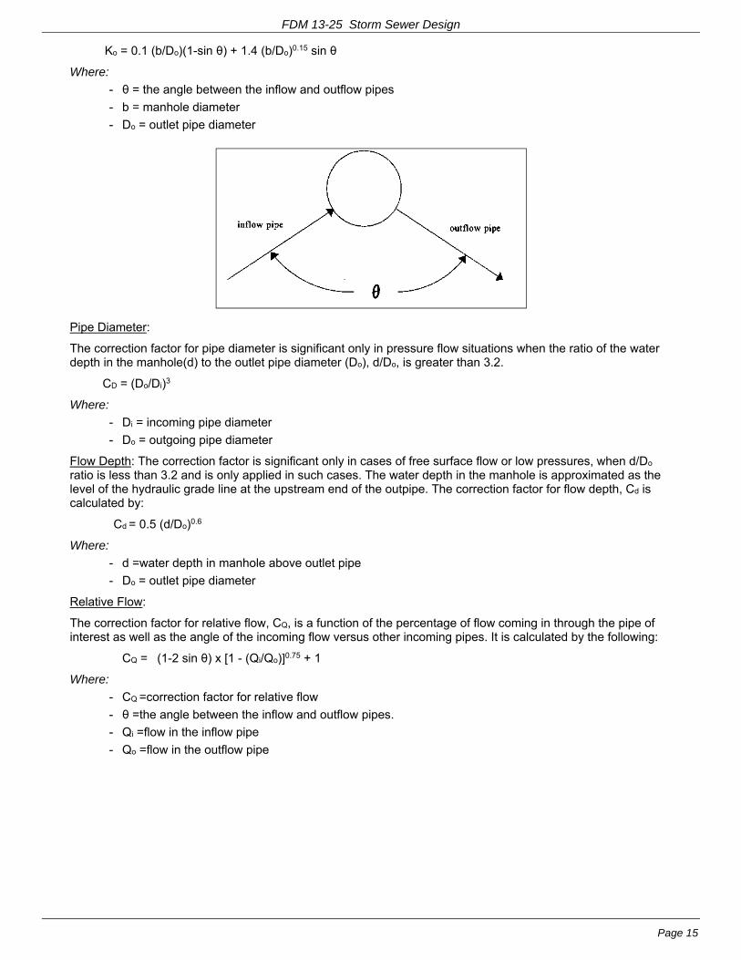
Ko = 0.1 (b/Do)(1-sin θ) + 1.4 (b/Do)0.15 sin θ

Where:

- θ = the angle between the inflow and outflow pipes

- b = manhole diameter

- Do = outlet pipe diameter

Pipe Diameter:

The correction factor for pipe diameter is significant only in pressure flow situations when the ratio of the water depth in the manhole(d) to the outlet pipe diameter (Do), d/Do, is greater than 3.2.

CD = (Do/Di)3

Where:

- Di = incoming pipe diameter

- Do = outgoing pipe diameter

Flow Depth: The correction factor is significant only in cases of free surface flow or low pressures, when d/Do ratio is less than 3.2 and is only applied in such cases. The water depth in the manhole is approximated as the level of the hydraulic grade line at the upstream end of the outpipe. The correction factor for flow depth, Cd is calculated by:

Cd = 0.5 (d/Do)0.6

Where:

- d =water depth in manhole above outlet pipe

- Do = outlet pipe diameter

Relative Flow:

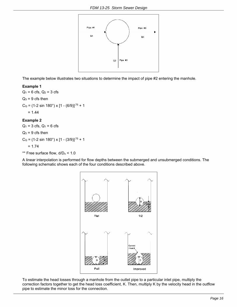
The correction factor for relative flow, CQ, is a function of the percentage of flow coming in through the pipe of interest as well as the angle of the incoming flow versus other incoming pipes. It is calculated by the following:

CQ = (1-2 sin θ) x [1 - (Qi/Qo)]0.75 + 1

Where:

- CQ =correction factor for relative flow

- θ =the angle between the inflow and outflow pipes.

- Qi =flow in the inflow pipe

- Qo =flow in the outflow pipe


The example below illustrates two situations to determine the impact of pipe #2 entering the manhole.

Example 1

Q1 = 6 cfs, Q2 = 3 cfs

Q3 = 9 cfs then

CQ = (1-2 sin 180°) x [1 - (6/9)].75 + 1

= 1.44

Example 2

Q1 = 3 cfs, Q1 = 6 cfs

Q3 = 9 cfs then

CQ = (1-2 sin 180°) x [1 - (3/9)].75 + 1

= 1.74

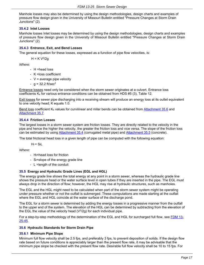
** Free surface flow, d/Do < 1.0

A linear interpolation is performed for flow depths between the submerged and unsubmerged conditions. The following schematic shows each of the four conditions described above.

To estimate the head losses through a manhole from the outlet pipe to a particular inlet pipe, multiply the correction factors together to get the head loss coefficient, K. Then, multiply K by the velocity head in the outflow pipe to estimate the minor loss for the connection.


Manhole losses may also be determined by using the design methodologies, design charts and examples of pressure flow design given in the University of Missouri Bulletin entitled "Pressure Changes at Storm Drain Junctions" (2).

35.4.2 Inlet Losses

Manhole losses Inlet losses may be determined by using the design methodologies, design charts and examples of pressure flow design given in the University of Missouri Bulletin entitled "Pressure Changes at Storm Drain Junctions" (2).

35.4.3 Entrance, Exit, and Bend Losses

The general equation for these losses, expressed as a function of pipe flow velocities, is:

H = K V2/2g

Where:

- H =head loss

- K =loss coefficient

- V = average pipe velocity

- g = 32.2 ft/sec2

Entrance losses need only be considered when the storm sewer originates at a culvert. Entrance loss coefficients Ke for various entrance conditions can be obtained from HDS #5 (3), Table 12.

Exit losses for sewer pipe discharging into a receiving stream will produce an energy loss at its outlet equivalent to one velocity head; K equals 1.0.

Bend loss coefficient Kb values for curvilinear and miter bends can be obtained from Attachment 35.6 and Attachment 35.7.

35.4.4 Friction Losses

The largest losses in a storm sewer system are friction losses. They are directly related to the velocity in the pipe and hence the higher the velocity, the greater the friction loss and vice versa. The slope of the friction loss can be estimated by using Attachment 35.4 (corrugated metal pipe) and Attachment 35.5 (concrete).

The total frictional head loss in a given length of pipe can be computed with the following equation:

Hf = SfL

Where:

- Hf=head loss for friction

- Sf=slope of the energy grade line

- L =length of the conduit

35.5 Energy and Hydraulic Grade Lines (EGL and HGL)

The energy grade line shows the total energy at any point in a storm sewer, whereas the hydraulic grade line shows the pressure head or the water surface level in open tubes if they are inserted in the pipe. The EGL must always drop in the direction of flow; however, the HGL may rise at hydraulic structures, such as manholes.

The EGL and the HGL might need to be calculated when part of the storm sewer system might be operating under pressure whether or not the outfall is submerged. These computations are made starting at the outfall where the EGL and HGL coincide at the water surface of the discharge pond.

The EGL for a storm sewer is determined by adding the energy losses in a progressive manner from the outfall to the upper end of the system. The elevation of the HGL can be determined by subtracting from the elevation of the EGL the value of the velocity head (V2/2g) for each individual pipe.

For a step-by-step methodology of the determination of the EGL and HGL for surcharged full flow, see FDM 13-25-45.

35.6 Hydraulic Standards for Storm Drain Pipe

35.6.1 Minimum Pipe Slope

Minimum full flow velocity shall be 2.5 fps, and preferably 3 fps, to prevent deposition of solids. If the design flow rate based on future conditions is appreciably larger than the present flow rate, it may be advisable that the minimum pipe slope be checked with the present flow rate. Desirable full flow velocity shall be 10 to 15 fps. For






some standard size concrete pipe (n = 0.013), the minimum slopes required to maintain a self-cleaning velocity of 2.5 or 3.0 fps at full flow are as follows:

Pipe Diameter (Inches)

Minimum Slope (Ft./Ft.)

2.5 fps 3.0 fps

12 .0030 .0044

15 .0023 .0032

18 .0018 .0025

24 .0012 .0017

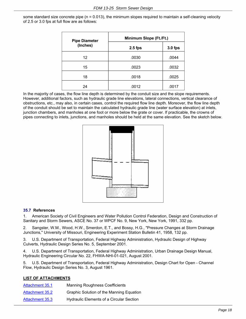
In the majority of cases, the flow line depth is determined by the conduit size and the slope requirements. However, additional factors, such as hydraulic grade line elevations, lateral connections, vertical clearance of obstructions, etc., may also, in certain cases, control the required flow line depth. Moreover, the flow line depth of the conduit should be set to maintain the calculated hydraulic grade line (water surface elevation) at inlets, junction chambers, and manholes at one foot or more below the grate or cover. If practicable, the crowns of pipes connecting to inlets, junctions, and manholes should be held at the same elevation. See the sketch below.

35.7 References

1. American Society of Civil Engineers and Water Pollution Control Federation, Design and Construction of Sanitary and Storm Sewers, ASCE No. 37 or WPCF No. 9, New York, New York, 1991, 332 pp.

2. Sangster, W.M., Wood, H.W., Smerdon, E.T., and Bossy, H.G., "Pressure Changes at Storm Drainage Junctions," University of Missouri, Engineering Experiment Station Bulletin 41, 1958, 132 pp.

3. U.S. Department of Transportation, Federal Highway Administration, Hydraulic Design of Highway Culverts, Hydraulic Design Series No. 5, September 2001.

4. U.S. Department of Transportation, Federal Highway Administration, Urban Drainage Design Manual, Hydraulic Engineering Circular No. 22, FHWA-NHI-01-021, August 2001.

5. U.S. Department of Transportation, Federal Highway Administration, Design Chart for Open - Channel Flow, Hydraulic Design Series No. 3, August 1961.

LIST OF ATTACHMENTS

Attachment 35.1 Manning Roughness Coefficients

Attachment 35.2 Graphic Solution of the Manning Equation

Attachment 35.3 Hydraulic Elements of a Circular Section





Attachment 35.4 Capacity and Velocity Diagram for Circular Corrugated Pipe Flowing Full (n = 0.024)

Attachment 35.5 Capacity and Velocity Diagram for Circular Concrete Pipe Flowing Full (n= 0.013)

Attachment 35.6 Sewer Bend Loss Coefficients

Attachment 35.7 Loss Coefficients for Miter Bends

FDM 13-25-40 Design Procedure: Full and Partially Full Flow August 8, 1997


The following procedure describes the hydrologic and hydraulic design of storm sewers operating under full or partially full flow conditions. For a detailed procedure on the design of storm sewers operating under a surcharged flow condition, see FDM 13-25-45.

40.2 Procedure

1. Prepare a set of prints or maps showing the entire drainage area contributing runoff to the proposed storm sewer.

2. Through the use of FDM 13-25-30, draw on the prints the design locations of all catch basins and inlets.

3. Locate trunk sewer and manholes on the plan; number manholes, catch basins, and inlets beginning from the upper end of the system; and assign a letter designation to each trunk line and lateral line beginning from the upper end of the system.

4. Tentatively sketch on the profile sheet a trunk sewer grade that is approximately parallel to the street profile.

5. The area contributing to each inlet or catch basin should:

- Be delineated on the map.

- Be numbered sequentially starting at the upper end of the system.

- Have its area measured in acres and marked on the map.

- Have a weighted runoff coefficient C estimated and marked on the map.

- Have the inlet time (time of concentration) estimated and marked on the map (minimum time of concentration must be five minutes).

6. Complete the work sheet, Attachment 40.1, for storm sewer design as follows:

a. Under the heading of "Location," enter the following:

- On the first line, the name of the street containing the sewer line.

- In column 1, the station of the upstream structure for the pipe run under consideration.

- In column 2, the structure type (M.H.-manhole, I-inlet, C.B.-catch basin) and the structure number of the upstream structure.

- In column 3, the structure type and the structure number of the downstream structure.

b. Under the heading entitled "Tributary Area,” enter the following:

- In column 4, the index number for each subarea.

- In column 5, the size in acres of each subarea.

- In column 6, the weighted runoff coefficient C for each subarea.

- In column 7, the equivalent area (product of columns 5 and 6) of each subarea.

- In column 8, the sum of all the equivalent areas for the pipe section under consideration.

c. Under the heading of "Travel Time," enter the following:

- In column 9, the inlet time for each subarea. For the first inlet of a system, the inlet time is the same as the time of concentration of the system. On subsequent inlets, the inlet time is equal to the time of concentration for each subarea. If the inlet time exceeds the time of concentration from the upstream basin, and the subarea tributary to the inlet is of sufficient magnitude, the inlet time should be substituted for the time of concentration and used for this and subsequent design points.

- In column 10 or column 11, the appropriate flow time between the upstream structure and the downstream structure. If a significant portion of the flow is carried by the street, the street flow time should be entered in column 10. However, pipe flow volume generally is







more significant than street flow volume, and hence pipe flow time is usually entered in column 11. If there is any question as to which is the controlling time, both times should be computed, entered, and compared (see e.8).

- In column 12, the time of concentration, which is the greater of:

- The sum of the previous design point (the inlet end of a pipe) time of concentration and the intervening flow time; or,

- The inlet time for the present design point.

d. Under the heading entitled "Rainfall-Runoff," enter the following:

- In column 13, average rainfall intensity for a rainfall duration equal to the time of concentration (column 12) and the selected design frequency. Obtain the rainfall intensity from the appropriate I-D-F curve, FDM 13-10-5, Attachment 5.4.

- In column 14, the direct runoff (product of columns 8 and 13).

- In column 15, other runoff, such as controlled releases from rooftops, parking lots, base flows from groundwater, and any other source.

- In column 16, the design runoff (summation of columns 14 and 15).

e. Use the columns under the heading of "Flow in Conduit" and the following procedure to design the conduit:

- Enter in column 17 a trial slope for the sewer pipe. Usually the slope of the roadway can be used.

- Determine from either FDM 13-25-35, Attachment 35.4, or FDM 13-25-35, Attachment 35.5 the pipe size by laying a straightedge between the discharge (column 16) and slope (column 17) scales. The appropriate size pipe is read directly above the straightedge. Enter the value in column 18.

- Adjust the straightedge on the nomograph so that it lies on the slope (column 17) and the pipe size (column 18). Read the capacity flowing full on the discharge scale. If this value is 10 percent larger than the design runoff (column 16), then, if feasible, the slope of sewer should be flattened. Through using the discharge (column 16) and pipe size (column 18) scales of the nomograph, a new slope at which the pipe just flows full can be read from the slope scale.

- If a pipe slope adjustment is made, reenter the new value in column 17.

- Enter in column 19 the capacity flowing full for the selected pipe and slope.

- Enter in column 20 the mean velocity flowing full by laying a straightedge on the slope (column 17) and pipe size (column 18) scales of the nomograph. This value should be greater than three fps.

- Enter in column 21 the length of pipe, which is equal to the distance between the center lines of the manholes.

- Enter in column 11 the pipe flow time determined by dividing the length (column 21) by the velocity (column 20). Convert from seconds to minutes.

- Enter in column 22 the fall of pipe.

f. Under the heading of "Vertical Control," enter the following:

- In column 23, the invert elevation for the upper end of the pipe.

- In column 24, the invert elevation for the lower end of the pipe.

- In column 25, the top of structure elevation for the upper end of the pipe.

- In column 26, the top of structure elevation for the lower end of the pipe.

40.2.1 Example Problem

This example problem shows the application of the above-outlined procedure to the design of a storm sewer system operating under full or partially full conditions. See Attachment 40.2 for a plan and profile layout of the proposed storm sewer system. The design computations are also shown in this Attachment and are self-explanatory by following the procedure previously outlined.

Since this is an example problem, only the sewer trunk line is designed for explanation purposes. In an actual problem, the lateral pipes as well as the inlets (see FDM 13-25-30) would have to be designed.







LIST OF ATTACHMENTS

Attachment 40.1 Work Sheet for Storm Sewer Design

Attachment 40.2 Full and Partially Full Sewer Design Problem

FDM 13-25-45 Design Procedure: Surcharged Full Flow August 8, 1997


The purpose of this procedure is to determine the effect of backwater on a storm sewer system or the effects of an existing underdesigned storm sewer system that operates in a surcharged condition. All storm sewers that will operate under a submerged condition shall be checked by this section to ensure that low points along the highway will not be inundated during the design storm.

45.2 Procedure

When a sewer system operates under a surcharged condition, the elevation of the water surface (hydraulic grade line - HGL) may be raised high enough to cause the water to bubble out of the manholes and inlets at low points in the highway grade. The elevation of the HGL is equal to the energy grade line (EGL) minus the velocity head. Therefore, the EGL, which is the total energy in the system (potential energy plus kinectic energy), must be calculated first. See Attachment 45.1 for the profiles, EGL's, and HGL's of two different storm sewer systems - one improperly designed (HGL above natural ground) and one properly designed (HGL below natural ground).

A discussion of the energy losses associated with surcharged flow is contained in FDM 13-25-35. For the sake of expediency, the following approximations of loss coefficient at junctions can be used:

1. A 90° turn in main line use 1.5 x velocity head

2. Through flow in main line use 0.2 x velocity head

3. Through flow with large lateral use 0.5 - 1.5 x velocity head

4. First inlet in system use 1.5 x velocity head

Each of the above conditions uses the velocity head of the downstream pipe.

If the calculations show inundation of the pavement during the design storm, the storm sewer system should be redesigned with larger pipe sizes, which reduces the pipe friction loss and hence lowers the HGL.

1. Initially, design the storm sewer system by FDM 13-25-40, "Design Procedure: Full and Partially Full Flow." Assume there is free outfall from the storm sewer.

2. Draw a profile of the proposed sewer showing the highway grade and the location of each manhole and each inlet, along with their cover elevations.

3. Use tabular design sheet "Work Sheet for Storm Sewer Design - Surcharged Flow," Attachment 45.2.

4. Under the heading of "Location," enter the following:

- In column 1, the station of the sewer outfall or the next structure.

- In column 2, the structure type (outfall, M.H.-manhole, I-inlet, C.B.-catch basin, etc.) and the structure number.

5. Under the heading entitled "Pipe Data,” enter the following:

- In column 3, the design discharge for the upstream pipe.

- In column 4, the pipe size of the upstream pipe.

- In column 5, the pipe length of the upstream pipe.

6. Under the heading of "Velocity Head," enter the following:

- In column 6, the mean pipe velocity of the upstream pipe.

- In column 7, the pipe velocity head (V12/2g) of the upstream pipe.

- In column 8, the mean channel velocity component in the outlet channel (which is parallel to the sewer). In most cases this can be considered negligible. This column is used only for the outflow pipe.

- In column 9, the channel velocity head for the velocity in column 8. In most cases this can be considered negligible. The outlet losses of the outlet pipe should be reduced by this amount.

7. Under the heading of "Pipe Head Losses," enter the following:






- In column 10, the bend loss coefficient K for any bends in this length of upstream pipe.

- In column 11, the bend energy loss (product of columns 7 and 10).

- In column 12, the friction slope as determined from FDM 13-25-35, Attachment 35.4 or FDM 13-25-35, Attachment 35.5 with the discharge (column 3) and the pipe size (column 4). This is the friction slope Sf of the EGL.

- In column 13 the friction head loss is obtained by multiplying (column 5) x (column 12)

8. Under the heading of "Structure Head Losses," enter the following:

- In column 14, the coefficient K for the appropriate structure losses (outlet, usually 1.00; inlet and manhole as discussed in this procedure and FDM 13-25-35).

- In column 15, the structure energy losses (product of column 7, pipe velocity head, and column 14, coefficient K structure). Note: Use the upstream pipe velocity head for an outlet structure and the downstream pipe velocity head for all other structure types.

9. Under the heading entitled "Grade Line Elevation at Structure,” enter the following:

- In the upper half of column 16, the downstream EGL elevation. For an outlet structure this is the surface elevation of the receiving body of water. However, for all other structures this elevation is the sum of the upstream EGL elevation of the previous structure (column 16), and the friction head loss (column 13) and the bend energy loss (column 11) of the interconnecting pipe.

- In the lower half of column 16, the upstream EGL elevation, which is the sum of the downstream EGL elevation (computed under 9a) and the structure energy losses (column 15).

- In the upper half of column 17, the downstream HGL elevation. For an outlet structure this is the surface elevation of the receiving body of water. However, for a manhole or an inlet this elevation is equal to the downstream EGL elevation (column 16) minus the downstream pipe velocity head (column 7).

- In the lower half of column 17, the upstream HGL elevation, which is equal to the upstream EGL elevation (column 16) minus the upstream pipe velocity head (column 7). This value is the water surface elevation within the structure.

10. Under the heading of "Vertical Control," enter the following:

- In column 18, the downstream and upstream invert elevations of the structure. These elevations will usually be the same unless the pipe size changes, and then the upstream elevation is equal to the change in pipe size plus the downstream invert elevation.

- In column 19, the top of structure elevation, which is the natural ground elevation or the street grade elevation.

- In column 20, the freeboard height, which is the difference of column 19 (top of structure elevation) and column 17 (upstream HGL elevation).

11. If the freeboard height is negative, the HGL elevation (water surface) is above the highway grade, and larger pipe sizes should be used downstream from the point of inundation in order to reduce the HGL elevation. The pipes should be enlarged sufficiently to allow at least one foot of freeboard at the most critical structure.

12. Repeat the procedure starting with step 4 for the next upstream structure.

13. If a free-water surface is encountered within the conduit, the calculations are normally suspended. However, if a structure further upstream has unusually high energy losses, thus producing surcharged flow, it may be necessary to continue the calculations using the surface of the normal depth of flow for the HGL within the conduit.

Theoretically, the energy losses for partially full flowing conduits should not be computed by the above-listed methods, which are only for full flowing conduits. However, for the sake of expediency it is recommended that the above-cited energy loss methodology for full flowing conduits also be applied to partially full flowing conduits.

Example Problem

This example problem is a continuance of the example problem from FDM 13-25-40, with the additional design control that the outfall is not a free fall outfall. Instead, a surcharged condition is produced through inundation of the outfall with a water elevation of 990.50. Therefore, the example storm sewer system designed by FDM 13-25-40 must be checked for surcharged flow starting with step 3 of the above-outlined design procedure.

See FDM 13-25-40, Attachment 40.2 for a plan and profile layout of the proposed storm sewer system designed






under full and partially full flow conditions. This figure satisfies steps l and 2 of the above-outlined design procedure for surcharged flow. The design computations for surcharged flow are shown in Attachment 45.3 of this procedure and are self-explanatory by following the design procedure outlined above. However, two highlights of this design example problem are:

1. The pipe between MH A-3 and A-4 is enlarged from a 36-inch to a 42-inch pipe to eliminate the popping of the cover of MH A-4; and,

2. The computations are discontinued at MH A-2, where a free water surface is encountered.

Since this is an example problem, only the sewer trunk line is checked for surcharged flow. However, in an actual design problem, the lateral inlets must also be checked for surcharged flow.

LIST OF ATTACHMENTS

Attachment 45.1 Energy and Hydraulic Grade Lines for a Properly and Improperly Designed Storm Sewer

Attachment 45.2 Work Sheet for Storm Sewer Design

Attachment 45.3 Example Work Sheet for Sewer Design Problem





FDM 13-25 Storm Sewer Design - Wisconsin Department of ...wisconsindot.gov/rdwy/fdm/fd-13-25.pdf ·...

Documents

Transcript of FDM 13-25 Storm Sewer Design - Wisconsin Department of ...wisconsindot.gov/rdwy/fdm/fd-13-25.pdf ·...