Investigation of a Hybrid HVDC System with DC Fault Ride ...

FAULT RIDE-THROUGH CAPABILITY OF MULTI-POLE PERMANENT MAGNET SYNCHRONOUS GENERATOR FOR WIND ENERGY CONVERSION SYSTEM by CLEMENT NDJEWEL KENDECK Thesis submitted in fulfilment of the requirements for the degree Master of Engineering: Electrical Engineering in the Faculty of Engineering at the Cape Peninsula University of Technology Supervisor: Dr AK Raji Bellville September 2019
CPUT copyright information The dissertation/thesis may not be published either in part (in scholarly, scientific or technical journals), or as a whole (as a monograph), unless permission has been obtained from the University

ii
DECLARATION
I, Clement Ndjewel Kendeck, declare that the contents of this dissertation/thesis represent
my own unaided work, and that the dissertation/thesis has not previously been submitted for
academic examination towards any qualification. Furthermore, it represents my own opinions
and not necessarily those of the Cape Peninsula University of Technology.
08 September 2019
Signed Date
iii
ABSTRACT
Wind has become one of the renewable energy technologies with the fastest rate of growth.
Consequently, global wind power generating capacity is also experiencing a tremendous
increase. This tendency is expected to carry on as time goes by, with the continuously
growing energy demand, the rise of fossil fuels costs combined to their scarcity, and most
importantly pollution and climate change concerns. However, as the penetration level
increases, instabilities in the power system are also more likely to occur, especially in the
event of grid faults. It is therefore necessary that wind farms comply with grid code
requirements in order to prevent power system from collapsing. One of these requirements is
that wind generators should have fault ride-through (FRT) capability, that is the ability to not
disconnect from the grid during a voltage dip. In other words, wind turbines must withstand
grid faults up to certain levels and durations without completely cutting off their production.
Moreover, a controlled amount of reactive power should be supplied to the grid in order to
support voltage recovery at the connection point.
Variable speed wind turbines are more prone to achieve the FRT requirement because of the
type of generators they use and their advanced power electronics controllers. In this
category, the permanent magnet synchronous generator (PMSG) concept seems to be
standing out because of its numerous advantages amongst which its capability to meet FRT
requirements compared to other topologies. In this thesis, a 9 MW grid connected wind farm
model is developed with the aim to achieve FRT according to the South African grid code
specifications. The wind farm consists of six 1.5 MW direct-driven multi-pole PMSGs wind
turbines connected to the grid through a fully rated, two-level back-to-back voltage source
converter. The model is developed using the Simpowersystem component of
MATLAB/Simulink. To reach the FRT objectives, the grid side controller is designed in such a
way that the system can inject reactive current to the grid to support voltage recovery in the
event of a grid low voltage. Additionally, a braking resistor circuit is designed as a protection
measure for the power converter, ensuring by the way a safe continuous operation during
grid disturbance.

iv
ACKNOWLEDGEMENTS
I would like to thank my supervisor Dr AK Raji for his guidance, patience, and
encouragements throughout this journey. I would not have made it this far without his
endless support.
I would also like to thank the management of Cape Peninsula University of Technology for
the material and financial support they have provided through University Research Funds
and bursaries grants.
I would also like to express my sincere gratitude to my lovely parents, brothers and sisters for
their continuous involvement in making my life a success.
To my friends and colleagues, I am also grateful for their moral support and
encouragements.
Lastly but not least, I would like to thank God for giving me all the strength and resources
necessary to successfully complete this degree.

v
DEDICATION
To my lovely parents

vi
TABLE OF CONTENTS
DECLARATION ..................................................................................................................... ii
ABSTRACT ........................................................................................................................... iii
ACKNOWLEDGEMENTS..................................................................................................... iv
DEDICATION ........................................................................................................................ v
TABLE OF CONTENTS ....................................................................................................... vi
LIST OF ABBREVIATIONS .................................................................................................. ix
LIST OF FIGURES ............................................................................................................... xi
LIST OF TABLES ................................................................................................................ xv
1 INTRODUCTION ............................................................................................................ 1
1.1 Background to the research problem ....................................................................... 1
1.2 Wind energy worldwide ............................................................................................ 2
1.3 Wind energy in South Africa .................................................................................... 3
1.4 Statement of the research problem .......................................................................... 4
1.5 Rationale and motivations of the research ............................................................... 5
1.6 Research aim and methodology .............................................................................. 5
1.7 Delineations of the research .................................................................................... 5
1.8 Thesis organisation .................................................................................................. 6
2 WIND TURBINE CONFIGURATIONS ............................................................................ 7
2.1 Components of wind turbines .................................................................................. 7
2.2 Wind turbine aerodynamics and characteristics ....................................................... 9
2.2.1 Power in the wind ............................................................................................. 9
2.2.2 Turbine power ................................................................................................... 9
2.2.3 Power coefficient and tip speed ratio .............................................................. 10
2.2.4 Power curve.................................................................................................... 10
2.3 Wind turbine aerodynamic controls ........................................................................ 12
2.3.1 Passive stall.................................................................................................... 12
2.3.2 Active stall ...................................................................................................... 12
2.3.3 Pitch control .................................................................................................... 13
2.4 Wind turbine topologies ......................................................................................... 13

vii
2.4.1 Wind turbines’ rotor configurations .................................................................. 13
2.4.2 Wind turbines’ generators ............................................................................... 14
2.4.3 Wind turbines rotational speed configurations................................................. 15
2.5 PMSG in variable speed wind turbines .................................................................. 19
2.5.1 Classification of PMSGs according to their flux orientation ............................. 20
2.5.2 Classification of PMSGs according to the magnet mounting ........................... 20
2.5.3 Classification of PMSGs according to the rotor position .................................. 23
2.5.4 Maximum power point tracking ....................................................................... 23
2.6 Power converters topologies for PMSG wind turbines ........................................... 26
2.6.1 Thyristor grid-side inverter .............................................................................. 26
2.6.2 Hard-switched grid-side inverter ..................................................................... 27
2.6.3 Multilevel converters ....................................................................................... 27
2.6.4 Matrix converters ............................................................................................ 28
2.6.5 Z-source converters ........................................................................................ 29
2.7 Power converter control ......................................................................................... 28
2.8 Summary of the chapter:........................................................................................ 30
3 GRID CODE REQUIREMENTS AND LVRT SOLUTIONS ............................................ 31
3.1 Grid code requirements for wind farms .................................................................. 31
3.1.1 Frequency and voltage operating range .......................................................... 33
3.1.2 Active power control ....................................................................................... 34
3.1.3 Reactive power and voltage control ................................................................ 35
3.1.4 Low Voltage Ride Through capability .............................................................. 35
3.1.5 South African grid code requirements for Renewable Power Plants ............... 39
3.2 LVRT methods for PMSG WTs .............................................................................. 40
3.2.1 Modified control-based techniques ................................................................. 40
3.2.2 Additional devices-based techniques .............................................................. 42
4 WIND TURBINE SYSTEM MODELING ........................................................................ 46
4.1 Wind turbine model ................................................................................................ 46
4.2 Drive train model ................................................................................................... 47
4.3 Modelling of the PMSG .......................................................................................... 48
viii
4.3.1 Reference frame theory .................................................................................. 51
4.3.2 Dynamic model ............................................................................................... 52
4.3.3 Steady state model ......................................................................................... 53
4.3.4 Equivalent circuit of the PMSG ....................................................................... 53
4.4 Modelling of the back-to-back voltage source converter ........................................ 54
4.4.1 Generator side converter control..................................................................... 57
4.4.2 Grid side converter control .............................................................................. 57
4.4.3 Space vector modulation (SVM) ..................................................................... 62
5 SIMULATION RESULTS AND DISCUSSIONS ............................................................. 69
5.1 Power system configuration ................................................................................... 69
5.2 Wind farm model aggregation ................................................................................ 70
5.3 Simulation results under normal operating conditions ............................................ 70
5.4 Simulation results under faulty conditions .............................................................. 77
5.4.1 Fault compensation ........................................................................................ 77
5.4.2 Case studies for simulations under grid faults ................................................. 81
6 CONCLUSIONS AND RECOMMENDATIONS ........................................................... 103
REFERENCES .................................................................................................................. 105
APPENDICES ................................................................................................................... 111
6.1 Appendix A: System parameters .......................................................................... 111
6.2 Appendix B: System simulation model ................................................................. 112

ix
LIST OF ABBREVIATIONS
AC Alternating Current
AFPM Axial Flux Permanent Magnet
BPA Blade Pitch Angle
CHB Cascaded H-Bridge
DC Direct Current
DFIG Doubly Fed Induction Generator
DPC Direct Power Control
DTC Direct Torque Control
DVR Dynamic Voltage Restorer
EESG Electrically Excited Synchronous Generator
ESS Energy Storage System
FACTS Flexible AC Transmission System
FC Flying Capacitor
FOC Field Oriented Control
FRT Fault Ride-Through
GSC Grid Side Converter
GWEC Global Wind Energy Council
HAWT Horizontal Axis Wind Turbine
HCC Hysteresis Current Control
IEA International Energy Agency
IEEE Institute of Electrical and Electronics Engineers
IGBT Insulated Gate Bipolar Transistor
IRP Integrated Resource Plan
IT Information Technology
LAB Lead Acid Battery
LVRT Low Voltage Ride-Through
MC Matrix Converter
MERS Magnetic Energy Recovery Switch
MPP Maximum Power Point
MPPT Maximum Power Point Tracking
MSC Machine Side Converter
NERSA National Energy Regulator of South Africa
NPC Neutral Point Clamping
OPC Optimum Power Control
OTC Optimum Torque Control
PCC Point of Common Coupling

x
PEC Power Electronics Converter
PI Proportional Integral
PLL Phase Locked Loop
PM Permanent Magnet
PMSG Permanent Magnet Synchronous Generator
PMSM Permanent Magnet Synchronous Machine
POC Point of Connection
PWM Pulse Width Modulation
RFPM Radial Flux Permanent Magnet
RPP Renewable Power Plant
RSA Republic of South Africa
SA South Africa
SCIG Squirrel Cage Induction Generator
SCR Silicon Controlled Rectifier
SSB Sodium Sulfur Battery
SSSC Static Synchronous Series Compensator
STATCOM Static Compensator
SVC Static Var Compensator
SVM Space Vector Modulation
SVPWM Space Vector Pulse Width Modulation
TCSC Thyristor Controlled Series Capacitor
TFPM Transversal Flux Permanent Magnet
THD Total Harmonic Distortion
THM Top Head Mass
TSR Tip Speed Ratio
UPFC Unity Power Factor Control
UK United Kingdom
US United States
VAWT Vertical Axis Wind Turbine
VOC Voltage Oriented Control
VSC Voltage Source Converter
VSI Voltage Source Inverter
WECS Wind Energy Conversion System
WPP Wind Power Plant
WRIG Wound Rotor Induction Generator
WT Wind turbine
WTS Wind turbine System
xi
LIST OF FIGURES
Figure 1.1: Global annual installed wind capacity (GWEC, 2015) .......................................... 2
Figure 1.2: Global cumulative installed wind capacity (GWEC, 2015) .................................... 3
Figure 1.3: Historic Eskom electricity price increases (Writer, 2015) ...................................... 4
Figure 2.1: Components of a wind turbine system ................................................................. 7
Figure 2.2: Power curve for a wind turbine ........................................................................... 11
Figure 2.3: Power curve for a passive stall-controlled wind turbine ...................................... 11
Figure 2.4: Power curve for an active stall and pitch-controlled wind turbine ........................ 12
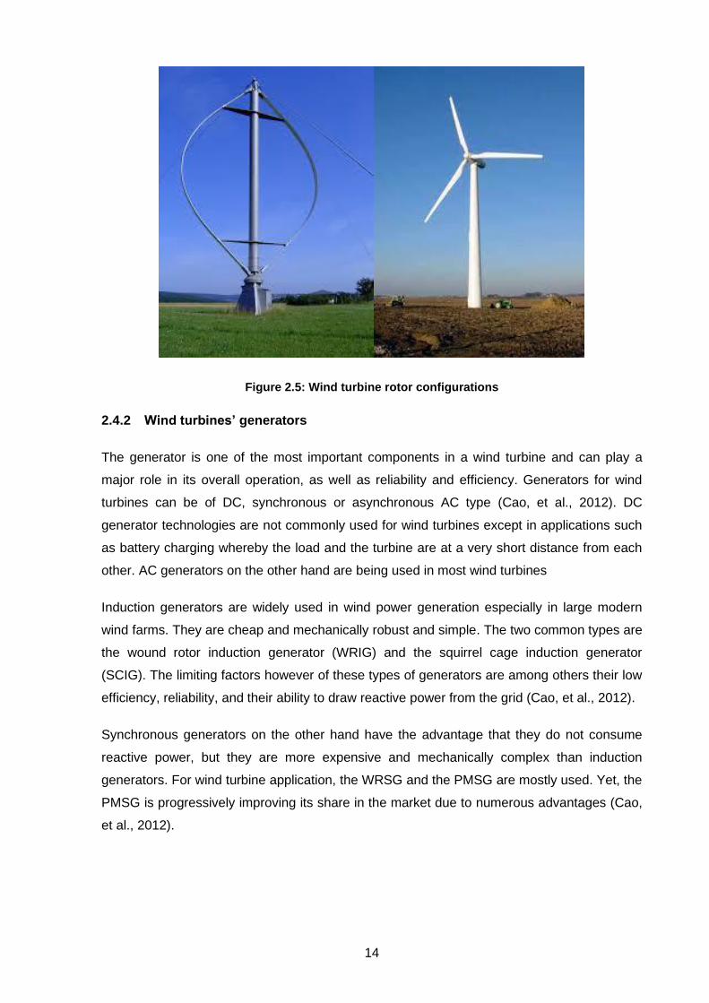
Figure 2.5: Wind turbine rotor configurations ....................................................................... 14
Figure 2.6: Classification of different wind turbine generators .............................................. 15
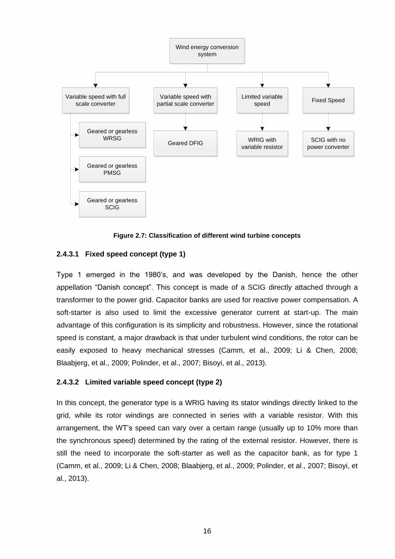
Figure 2.7: Classification of different wind turbine concepts ................................................. 16
Figure 2.8: Fixed speed concept .......................................................................................... 17
Figure 2.9: Limited variable speed concept .......................................................................... 17
Figure 2.10: Variable speed concept with partial scale converter ......................................... 17
Figure 2.11: Variable speed with full scale converter ........................................................... 18
Figure 2.12: Variable speed with direct grid connection ....................................................... 18
Figure 2.13: Cross sectional view in axial direction of axial flux (left) and radial flux (right)
PMSG .................................................................................................................................. 22
Figure 2.14: Surface mounted (left) and inset (right) magnet rotors for PMSG ..................... 22
Figure 2.15: Inner (left) and outer (right) rotor PMSG ........................................................... 22
Figure 2.16: Typical MPPT curve for a power versus rotational speed turbine characteristics
............................................................................................................................................ 23
Figure 2.17: PSF method applied to a PMSG based WECS ................................................ 24
Figure 2.18: Optimal TSR method applied to a PMSG based WECS ................................... 24
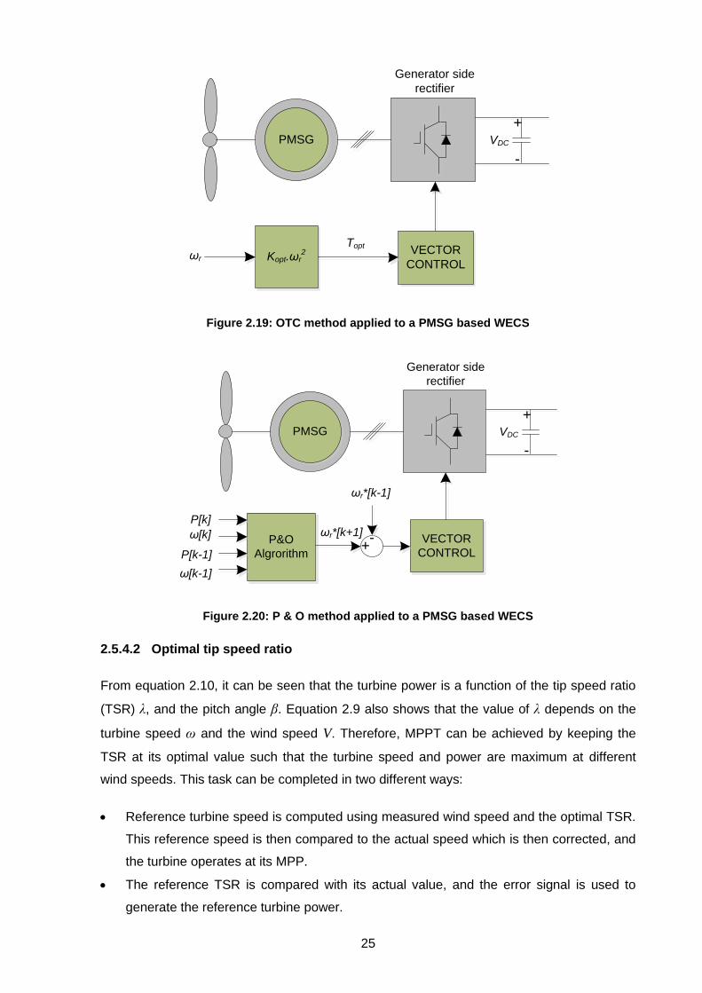
Figure 2.19: OTC method applied to a PMSG based WECS ................................................ 25
Figure 2.20: P & O method applied to a PMSG based WECS .............................................. 25
Figure 2.21: Examples of PECs used with PMSG based WECS .......................................... 28
Figure 3.1: Voltage and frequency operating ranges as defined by German power system
operator (Mohseni & Islam, 2012) ........................................................................................ 32
Figure 3.2: Frequency operating limits in some of the European countries .......................... 32
Figure 3.3: Active power regulation strategies (de Alegria, et al., 2007) ............................... 33
Figure 3.4: Power-frequency response curve by Danish grid code (Mohseni & Islam, 2012) 36
Figure 3.5: Reactive power and power factor requirement as enforced by Danish grid code
(Mohseni & Islam, 2012) ...................................................................................................... 36
Figure 3.6: Reactive power support requirement as defined by German grid code (Mohseni &
Islam, 2012) ......................................................................................................................... 37
Figure 3.7: German LVRT requirement (Mohseni & Islam, 2012) ......................................... 37
xii
Figure 3.8: South African LVRT curve (Mchunu & Khoza, 2013) .......................................... 38
Figure 3.9: Requirement for reactive power support during grid fault according to the South
African grid code (Mchunu & Khoza, 2013) .......................................................................... 38
Figure 3.10: LVRT enhancement techniques ....................................................................... 41
Figure 3.11: Block diagram of a typical BPA controller ......................................................... 41
Figure 3.12: Braking chopper configuration .......................................................................... 43
Figure 3.13: Energy storage system connected to the DC-link ............................................. 43
Figure 3.14: Typical structure of a STATCOM...................................................................... 43
Figure 3.15: Typical configuration of a dynamic voltage restorer .......................................... 44
Figure 3.16: Typical configuration of a unified power flow controller ..................................... 44
Figure 4.1: PMSG based wind turbine system ..................................................................... 47
Figure 4.2: Power coefficient as a function of tip speed ratio (Perelmuter, 2013) ................. 47
Figure 4.3: Drive train schematic modelling ......................................................................... 48
Figure 4.4: Representation of a 2-pole, 3-phase, star connected PMSG .............................. 49
Figure 4.5: Phasor diagram of a PMSG ............................................................................... 50
Figure 4.6: Simplified equivalent circuits of PMSG ............................................................... 53
Figure 4.7: Machine side rectifier ......................................................................................... 54
Figure 4.8: Grid side inverter ................................................................................................ 54
Figure 4.9: Power flow in the WTS ....................................................................................... 55
Figure 4.10: Direction of power flowing through the inverter................................................. 56
Figure 4.11: Phasor diagram of the field-oriented control ..................................................... 56
Figure 4.12: Generator side converter control ...................................................................... 58
Figure 4.13: Grid side converter control ............................................................................... 59
Figure 4.14: Two-level voltage source converter topology ................................................... 61
Figure 4.15: Space vector diagram of the two-level inverter ................................................. 62
Figure 4.16: Space vector diagram of the grid side inverter ................................................. 65
Figure 4.17: Seven-segment switching sequence for reference vector located in sector I .... 67
Figure 5.1: Single line diagram of the electric power system under study ............................ 69
Figure 5.2: Wind speed profile ............................................................................................. 71
Figure 5.3: Generator speed ................................................................................................ 71
Figure 5.4: Turbine mechanical torque ................................................................................. 71
Figure 5.5: Wind turbine's power coefficient ......................................................................... 72
Figure 5.6: Wind turbie's tip speed ratio ............................................................................... 72
Figure 5.7: Three phase stator voltages ............................................................................... 72
Figure 5.8: Three phase stator currents ............................................................................... 73
Figure 5.9: Stator active power ............................................................................................ 73
Figure 5.10: d and q-axis stator currents with references ..................................................... 74
Figure 5.11: Three-phase grid voltages................................................................................ 74
xiii
Figure 5.12: Three phase grid currents ................................................................................ 74
Figure 5.13: DC-link voltage ................................................................................................. 75
Figure 5.14: Current through DC-link ................................................................................... 75
Figure 5.15: DC-link power .................................................................................................. 75
Figure 5.16: d and q-axis grid currents with references ........................................................ 76
Figure 5.17: Grid active power ............................................................................................. 76
Figure 5.18: Reactive power to the grid ............................................................................... 76
Figure 5.19: Grid frequency ................................................................................................. 77
Figure 5.20: Block diagram of the pitch angle controller ....................................................... 78
Figure 5.21: DC-link protection scheme ............................................................................... 79
Figure 5.22: Grid reactive power support scheme ................................................................ 80
Figure 5.23: Voltage profile during fault at bus 3 for case 1.................................................. 81
Figure 5.24: Voltage profile at PCC during grid fault for case 1 ............................................ 82
Figure 5.25: Grid active power output during grid fault for case 1......................................... 82
Figure 5.26: DC-link voltage during grid fault for case 1 ....................................................... 83
Figure 5.27: Grid reactive power output during grid fault for case 1 ..................................... 83
Figure 5.28: Voltage profile during fault at bus 3 for case 2.................................................. 84
Figure 5.29: Voltage profile at PCC during grid fault for case 2 ............................................ 84
Figure 5.30: Grid active power output during grid fault for case 2......................................... 85
Figure 5.31: DC-link voltage during grid fault for case 2 ....................................................... 86
Figure 5.32: Grid reactive power output during grid fault for case 2 ..................................... 86
Figure 5.33: Voltage profile during fault at bus 3 for case 3.................................................. 87
Figure 5.34: Voltage profile at PCC during grid fault for case 3 ............................................ 87
Figure 5.35: Grid active power output during grid fault for case 3......................................... 88
Figure 5.36: DC-link voltage during grid fault for case 3 ....................................................... 88
Figure 5.37: Grid reactive power output during grid fault for case 3 ..................................... 89
Figure 5.38: Voltage profile during fault at bus 3 for case 4.................................................. 89
Figure 5.39: Voltage profile at PCC during grid fault for case 4 ............................................ 90
Figure 5.40: Grid active power output during grid fault for case 4......................................... 90
Figure 5.41: DC-link voltage during grid fault for case 4 ....................................................... 91
Figure 5.42: Grid reactive power output during grid fault for case 4 ..................................... 91
Figure 5.43: Voltage profile during fault at bus 3 for case 5.................................................. 92
Figure 5.44: Voltage profile at PCC during grid fault for case 5 ............................................ 92
Figure 5.45: Grid active power output during grid fault for case 5......................................... 93
Figure 5.46: DC-link voltage during grid fault for case 5 ....................................................... 93
Figure 5.47: Grid reactive power output during grid fault for case 5 ..................................... 94
Figure 5.48: Voltage profile during fault at bus 3 for case 6.................................................. 94
Figure 5.49: Voltage profile at PCC during grid fault for case 6 ............................................ 95
xiv
Figure 5.50: Grid active power output during grid fault for case 6......................................... 95
Figure 5.51: DC-link voltage during grid fault for case 6 ....................................................... 96
Figure 5.52: Grid reactive power output during grid fault for case 6 ..................................... 96
Figure 5.53: Voltage profile during fault at bus 3 for case 7.................................................. 97
Figure 5.54: Voltage profile at PCC during grid fault for case 7 ............................................ 97
Figure 5.55: Grid active power output during grid fault for case 7......................................... 98
Figure 5.56: DC-link voltage during grid fault for case 7 ....................................................... 98
Figure 5.57: Grid reactive power output during grid fault for case 7 ..................................... 99
Figure 5.58: Voltage profile during fault at bus 1 for case 8.................................................. 99
Figure 5.59: Voltage profile at PCC during grid fault for case 8 .......................................... 100
Figure 5.60: Grid active power output during grid fault for case 8....................................... 100
Figure 5.61: DC-link voltage during grid fault for case 8 ..................................................... 101
Figure 5.62: Grid reactive power output during grid fault for case 8 ................................... 101
Figure B.6.1: Electric power system model ........................................................................ 113
Figure B.6.2: Complete model of the PMSG wind energy conversion system .................... 114
Figure B.6.3: Simulation model of the generator side converter ......................................... 115
Figure B.6.4: Simulation model of the grid side converter .................................................. 116

xv
LIST OF TABLES
Table 2.1: Comparison of different wind turbine concepts .................................................... 21
Table 3.1: Classification of RPPs according their rated power (Mchunu & Khoza, 2013) ..... 39
Table 4.1: Switching states and output voltages of the inverter ............................................ 63
Table 4.2: Space vectors, switching states, and vectors definition ....................................... 64
Table 4.3: Relationship between reference vector location and dwell times ......................... 66
Table 4.4: Seven segment switching sequence ................................................................... 67
Table A.1: Individual wind turbine parameters ................................................................... 111
Table A.2: Generator parameters....................................................................................... 111
Table A.3: DC-link parameters ........................................................................................... 111

1
CHAPTER ONE
1 INTRODUCTION
1.1 Background to the research problem
There is no secret about the importance of electricity in the modern industrialized world.
Electricity is needed for lighting, telecommunications, IT, cooking, transportation, or even for
medical purposes, just to name but a few. In fact, contemporary society tends to depend
completely upon electricity at such an extent that it will be difficult to even imagine life without
electricity (Breeze, 2005).
One of the largest industries in the world is certainly the industry of power generation. Its
environmental impact is just as much important, with pollution and climate change associated
to the burning of fossil fuels, which constitute without any doubt the most used energy
sources for electricity generation in the world (Breeze, 2005).
The use of nuclear energy for electricity generation could eventually help contain and even
reduce at long term the global carbon emission. However, there are concerns about not only
the disposal of radioactive waste, but also the safety of nuclear reactors. A very fresh and
concrete example is the Fukushima nuclear disaster which took place on March 11, 2011
(Basrur & Koh, 2012).
On the other hand, with demographic growth and social and economic development, the
global energy supply will continue to rise in order to satisfy global energy demand. The
International Energy Agency (IEA, 2012) predicts a 1.7 billion increase in world’s population
between 2010 and 2035, and consequently about 37% increase in global energy demand
over the same period.
Taking all these issues into consideration, it is clear that the power generation industry can
no longer simply rely on traditional means of electricity generation to achieve clean, reliable
and sustainable energy supply. Therefore, the need to consider alternative energy supply
technologies is imperious.
Renewable energy sources, due to their abundance and cleanliness, seem to be able to
provide both the environmental and energy security that fossil fuels cannot guaranty (Tong,
2010). However, cost issues still make many governments reluctant to engage towards
renewables, although majority of people, including researchers, find them very attractive and
full of benefits (Craddock, 2008).
2
Over the past decade, the research industry has paid a particular attention to wind energy
among all other renewable energy sources. This interest has resulted in the fast emergence
of various wind generators and power electronics converters technologies, leading to a major
boost in terms of the global wind power production capacity.
However, transient stability and power quality issues are important challenges that come with
this increasing penetration level of wind power in the power system (Ali, 2012). As such, wind
turbines are nowadays expected to behave like conventional power plants and should
therefore meet certain connection requirements for safe and reliable grid connection. Some
of these requirements include frequency and voltage control, as well as fault ride-through
(FRT) capability (Patel, 2006).
1.2 Wind energy worldwide
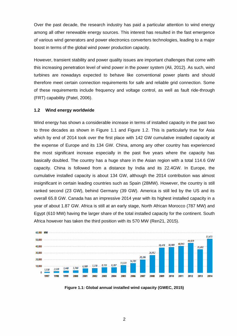
Wind energy has shown a considerable increase in terms of installed capacity in the past two
to three decades as shown in Figure 1.1 and Figure 1.2. This is particularly true for Asia
which by end of 2014 took over the first place with 142 GW cumulative installed capacity at
the expense of Europe and its 134 GW. China, among any other country has experienced
the most significant increase especially in the past five years where the capacity has
basically doubled. The country has a huge share in the Asian region with a total 114.6 GW
capacity. China is followed from a distance by India and its 22.4GW. In Europe, the
cumulative installed capacity is about 134 GW, although the 2014 contribution was almost
insignificant in certain leading countries such as Spain (28MW). However, the country is still
ranked second (23 GW), behind Germany (39 GW). America is still led by the US and its
overall 65.8 GW. Canada has an impressive 2014 year with its highest installed capacity in a
year of about 1.87 GW. Africa is still at an early stage, North African Morocco (787 MW) and
Egypt (610 MW) having the larger share of the total installed capacity for the continent. South
Africa however has taken the third position with its 570 MW (Ren21, 2015).
Figure 1.1: Global annual installed wind capacity (GWEC, 2015)

3
Figure 1.2: Global cumulative installed wind capacity (GWEC, 2015)
1.3 Wind energy in South Africa
In 2014, South Africa had finally taken a serious option into the wind industry with its 560 MW
capacity installed over the year. This obviously represents a tremendous step forward
considering that it took about a decade for the country to see its first 10 MW installed.
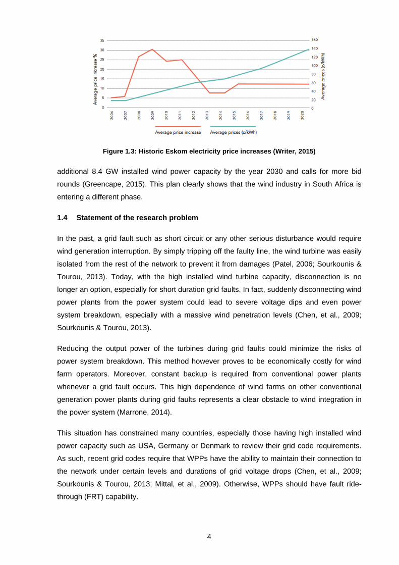
For many years, South Africa has completely relied on fossil fuels for electricity generation,
88% of the power produced coming from coal. This is completely understandable provided
the country hosts one of the largests coal deposits in the world. However, the price of
electricity keeps increasing as illustrated in Figure 1.3, and the population is still suffering
from the consequences of multiple power blackouts (GWEC, 2015).
As part of a solution to the country’s energy crisis, the South African government has
decided to shift towards renewable energies, essentially through its REIPPPP (Renewable
Energy Independent Power Producer Procurement Program). This program was established
in 2011 with the aim of promoting the rapid expansion of renewable energy in the South
African electricity market, without risks of excessive losses due to overpricing in case of a
single power producer. This would be done by allocating different projects to different
independent power producers over five round bids. Since then, over 5 GW have already
been allocated in four rounds, of which about 1.5 MW is already supplying to the national grid
(Greencape, 2015).
As far as wind energy is concerned, 2660 MW have already been allocated with 660 MW
remaining for the last round. Wind energy has the highest allocation so far, followed by solar
energy. The year 2014 saw the first results from the REIPPPP with some of the first bid wind
farms coming into operation (Greencape, 2015). Currently operating large wind farms in
South Africa include Sere (100 MW), Cookhouse (138.6 MW), Jeffreys Bay (138 MW)
Nobelsfontein (73.8 MW) and more (Writer, 2015).
The integration of wind energy through the REIPPPP has so far been successful and shows
promising future. For this reason, the Integrated Resource Plan (IRP) has planned for an
4
Figure 1.3: Historic Eskom electricity price increases (Writer, 2015)
additional 8.4 GW installed wind power capacity by the year 2030 and calls for more bid
rounds (Greencape, 2015). This plan clearly shows that the wind industry in South Africa is
entering a different phase.
1.4 Statement of the research problem
In the past, a grid fault such as short circuit or any other serious disturbance would require
wind generation interruption. By simply tripping off the faulty line, the wind turbine was easily
isolated from the rest of the network to prevent it from damages (Patel, 2006; Sourkounis &
Tourou, 2013). Today, with the high installed wind turbine capacity, disconnection is no
longer an option, especially for short duration grid faults. In fact, suddenly disconnecting wind
power plants from the power system could lead to severe voltage dips and even power
system breakdown, especially with a massive wind penetration levels (Chen, et al., 2009;
Sourkounis & Tourou, 2013).
Reducing the output power of the turbines during grid faults could minimize the risks of
power system breakdown. This method however proves to be economically costly for wind
farm operators. Moreover, constant backup is required from conventional power plants
whenever a grid fault occurs. This high dependence of wind farms on other conventional
generation power plants during grid faults represents a clear obstacle to wind integration in
the power system (Marrone, 2014).
This situation has constrained many countries, especially those having high installed wind
power capacity such as USA, Germany or Denmark to review their grid code requirements.
As such, recent grid codes require that WPPs have the ability to maintain their connection to
the network under certain levels and durations of grid voltage drops (Chen, et al., 2009;
Sourkounis & Tourou, 2013; Mittal, et al., 2009). Otherwise, WPPs should have fault ride-
through (FRT) capability.

5
It is therefore important to investigate, through computer simulations and/or hardware
experiments, how FRT can be achieved in accordance to grid code specifications, especially
with evolving wind generator technologies such as PMSG.
1.5 Rationale and motivations of the research
South Africa is aware of its tremendous wind resource. Even though the country’s wind
generation is still at a growing phase, SA intends to become one of the countries with most
activities in the sector of wind development in the near future. This rapid growth should
obviously accommodate with the latest and also most efficient technologies in order to
ensure safe and reliable energy supply.
Wind industry is experiencing many changes, especially regarding drive-train technologies
(Wenske, 2011). As such, direct driven wind turbines equipped with PMSGs are becoming
more attracting and their market share is also increasing, due to their multiple advantages
over other drive-train topologies (Wenske, 2011; Sanchez, et al., 2012; Gupta, et al., 2012).
With the increasing penetration of PMSG in the world’s wind market, a massive investigation
into the compliance of this type of generator with different grid codes requirements is
necessary. South Africa is an emerging wind power country and therefore such study needs
to be carried through in order to facilitate wind integration. According to Sourkounis & Tourou
(2013), FRT and more specifically low voltage ride through (LVRT), is the most important grid
code requirement for wind farms. This explains the choice of this topic for the research.
1.6 Research aim and methodology
The aim of this research is to achieve FRT capability with a multiple-pole PMSG grid
connected WECS according to South African grid code requirements. In order to achieve this
goal, the following tasks must be completed:
• Modelling and Analysis of the PMSG based wind turbine system
• Implementation of the electric power system benchmark
• Design of the control system to achieve FRT of multi-pole PMSG
• Implementation of LVRT control on wind turbine system for different grid faults
• Analysis and interpretation of simulated and experimental results
1.7 Delineations of the research
In this research, the LVRT capability of a multi-pole PMSG is investigated according to South
African grid code requirements. Simulation studies are carried through with emphasis on the
case of symmetrical faults which are the most severe types.

6
1.8 Thesis organisation
This thesis is organised in seven chapters. Chapter one, the introduction gives an overview
of the evolution of wind energy at global and national levels. The importance of this research
as well as its aim and contributions are well defined. Research methods and thesis
organisation are discussed. The second chapter is a review of different wind turbine
configurations. The chapter firstly describes different components available in typical wind
turbine systems. Then, different rotor, generator, drive-train, and power converter topologies
are discussed and compared. Aerodynamic and electrical control strategies are also
discussed. In the third chapter, grid code requirements and LVRT solutions are discussed.
The E-on, Danish and South African grid codes are elaborated. The LVRT requirement is
well explained and common LVRT enhancement methods are discussed and compared. The
fourth chapter presents a detailed modelling of the wind turbine system as well as power
system benchmark used. Chapter five shows the implementation of the LVRT strategies
used in this thesis Simulation results are presented, analysed and interpreted in chapter six.
Conclusions are drawn in the chapter seven. Recommendation for further improvement of
the research or inspection of other aspects are also given at the end of this chapter.

7
CHAPTER TWO
2 WIND TURBINE CONFIGURATIONS
Introduction
This chapter is an overview of the different wind turbine concepts available and currently
used in the market. In fact, with recent advances in science and technology, many turbine
topologies have evolved over the years, each one trying to overcome the previous shortfalls.
This has led to significant improvements in terms of wind energy harvesting, structural
strength, energy efficiency (mechanical and electrical), and overall reliability of wind turbines,
to guarantee safe and reliable supply at lower cost.
The wind turbine topology used in this thesis was chosen based on certain criteria after
comparing the other topologies. In this chapter, a review of some of the most common wind
turbine concepts is presented. Firstly, the basic components of a wind turbine are presented
with their functions explained. Then follows are explanation of the aerodynamic operating
principles, and finally a comparison of the different wind turbine concepts according to their
rotor, generator, and power electronics concepts.
2.1 Components of wind turbines
Figure 2.1: Components of a wind turbine system

8
The major components that constitute a wind turbine are represented in Figure 2.1. They can
be grouped into five main sections namely the rotor, the drive train, the frame, the yaw
system and the tower. Some of the components are discussed below (Manwell, et al., 2009;
Wu, et al., 2011; Hansen, 2008).
The rotor
The rotor is the part responsible for the extraction of wind power to be converted into
rotational movement in order for the turbine to generate electrical power. The turbine blades,
the hub, and the aerodynamic control surfaces essentially constitute the rotor of a wind
turbine.
The blades
The blades create the torque needed for the wind turbine to produce useful electrical power
from the wind blow. The blades must be designed in such a way that their shape and
material facilitate not only maximum extraction of wind energy, but also sufficiently withstand
physical stress caused by strong winds and excessive loads.
The hub
The hub is the part that links the turbine’s shaft to the blades and transmits the torque
produced to the drive train.
The drive-train
The drive-train includes all rotating components, the main shaft, gearbox, brakes, and
generator.
The brakes
Brakes are used to block the rotor from rotating, to allow maintenance on the wind turbine or
in case of emergency whenever there is a fault on the turbine itself or even in the power
system.
The main shaft
Also called low speed shaft, the main shaft transfers the rotational force from the blades to
the remainder of the drive train.
The gearbox
This component multiplies the low speed from the main shaft to match the generator’s high
speed shaft (mostly 1500rpm and 1800rpm). Due to its weight, price, and need for constant
maintenance the gearbox is becoming less desirable in modern wind turbines.
The generator
The generator is the electrical machine that converts the mechanical rotational power from
the main shaft into electrical power to be supplied to load.
The yaw system
The yaw system has the mission to ensure that the turbine faces the wind, allowing
maximum energy to be extracted.

9
The nacelle
The nacelle is the frame that contains the shaft, the gearbox, the generator, and many other
parts.
The tower
The tower is the structure that supports all the nacelle components in altitude, allowing the
blades to freely sweep the wind over their diameter without risks of crashing on the ground.
Anemometers (wind sensors)
Wind sensors measure the speed as well as the direction of the wind necessary for blade
orientation at different.
2.2 Wind turbine aerodynamics and characteristics
2.2.1 Power in the wind
The energy available in the wind can be expressed as (Wagner & Mathur, 2009)
2
2
1mVEwind =
Equation 2.1
where m represents a certain mass of air flowing at wind speed V. this mass of air is
proportional to the air density ρ, the area swept by the blades A, and the wind speed V over a
specific period of time t, and can further be expressed as:
AVtm = Equation 2.2
Equation 2.2 can be substituted in into Equation 2.1 and the following expression for the
energy in the wind is obtained:
tAVEwind
3
2
1=
Equation 2.3
Since
t
EP wind
wind = Equation 2.4
The power available in the wind can thus be given as:
3
2
1AVPwind =
Equation 2.5
2.2.2 Turbine power
As it can be seen in Equation 2.5 above, the wind power is proportional to the air density, the
wind speed, and the area of the wind turbine rotor. However, not all the power in wind is
used by the wind turbine. According to the Betz limit, only a fraction (approximately 59.3%) of

10
the wind power can be extracted by the wind turbine and is known as Power Coefficient (Cp).
Therefore, the maximum power extracted from the wind is given as (Ackermann, 2005):
pturbine CAVP 3
2
1=
Equation 2.6
2.2.3 Power coefficient and tip speed ratio
Equation 2.6 above can be rewritten as:
pwindturbine CPP = Equation 2.7
Making Cp the subject of the formula, the power coefficient can be expressed as:
wind
turbinep
P
PC =
Equation 2.8
From the previous expression, the power coefficient can be defined as the ratio of the power
extracted by the turbine blades to the available power in the wind. The power coefficient can
also be seen as the efficiency of the rotor blades (Wagner & Mathur, 2009).
The tip speed ratio is the ratio of the rotor’s speed at the tip of the blade and the wind speed
and is expressed as:
V
r =
Equation 2.9
where r is the radius of the turbine’s rotor blade, and ω the rotating speed of the blade.
The power coefficient being a function of λ and β, the turbine power can also be written as:
( ) ,2
1 3
pturbine CAVP = Equation 2.10
2.2.4 Power curve
The power curve is an important characteristic of wind turbines. The power curve shows the
expected output power produced by a turbine at different wind speeds. Figure 2.2 below
represents a typical power curve for a wind turbine. As illustrated, there are three wind speed
limits that determine the shape of the power curve: the cut-in speed, the cut-out speed, and
the rated speed. The cut-in speed is the minimum wind speed at which the turbine starts
producing power and usually ranges between 2 to 5 m/s. At wind speeds below this value,
not sufficient torque is produced to cause effective rotation of the turbine; no output power is
thus produced. The rated speed represents the wind speed at which rated power will be
produced by the wind turbine and ranges between 12 and 15 m/s. At wind speeds above
rated value, the output power is usually maintained constant using aerodynamic control
mechanisms. The cut-out speed on the other hand is the value above which the turbine may

11
start experiencing turbulences which could lead to damage. This value usually revolves
around 25 m/s. As shown figure 2.2, passed the cut-out speed, the wind turbine will
automatically stop its operation and enter a park mode (Wagner & Mathur, 2009; Wu, et al.,
2011).
Cut-in Cut-outRated Wind speed
(m/s)
Mechanical
power
Operating region
Rated
power
Min
power
Parking
mode
Parking
mode
Theoretical
power curve
Generator
control
Aerodynamic
control
Figure 2.2: Power curve for a wind turbine
Cut-in Cut-outRated Wind speed
(m/s)
Mechanical
power
Rated
power
Min
power
Passive stall
Figure 2.3: Power curve for a passive stall-controlled wind turbine

12
Cut-in Cut-outRated Wind speed
(m/s)
Mechanical
power
Rated
power
Min
power
Active stall/pitch control
Figure 2.4: Power curve for an active stall and pitch-controlled wind turbine
2.3 Wind turbine aerodynamic controls
The aerodynamic control of wind turbines is important in order to maximize the amount of
power to be extracted from the wind, without exposing the turbine to extreme wind conditions
that could affect its operation and eventually cause damage or destruction. There are three
common methods namely passive stall, active stall, and pitch control.
2.3.1 Passive stall
Passive stall is the simplest and easiest wind turbine aerodynamic control. The amount of
energy extracted during high wind speeds conditions is reduced by stalling of the blades,
without change of their geometry. The turbine blades are fixed on the hub such that they can
only slightly twist around their longitudinal axis. The main difficulty in passive stall control
remains the blade design which requires very precise aerodynamic properties of the blades
to ensure more effective stall effect (Wagner & Mathur, 2009; Earnest, 2015; Munteanu, et
al., 2008).
2.3.2 Active stall
In Active stall control, the blades are turned into the direction of the wind to stall. As opposed
to passive stall, the blades can completely rotate around their longitudinal axis. The principal
advantage over pitch control is that active stall only requires small pitch rate changes to
maintain rated power output. Another advantage is the reduced strain on the generator
during high wind conditions (Wagner & Mathur, 2009; Earnest, 2015; Munteanu, et al., 2008).

13
2.3.3 Pitch control
In pitch control the blades are deviated out of the direction of the wind to reduce the power
captured, eventually slowing down the turbine whenever the wind speed goes beyond its
rated value. Pitch control is similar to active stall only that the blades are turned into the wind
direction in active stall. Moreover, the pitch system has to act quickly, in order to limit power
excursions, due to their large range of pitch angles for rated power output control. However,
the pitch control presents numerous advantages over stall control such as increased energy
capture, ease in aerodynamic braking, and overload reduction when the turbine is shut down
(Wagner & Mathur, 2009; Earnest, 2015; Munteanu, et al., 2008).
2.4 Wind turbine topologies
Generally, WTs classifications are made according to the rotor configurations, the generator
technologies, and the turbine’s rotational speed (Ackermann, 2005; Hau, 2013).
2.4.1 Wind turbines’ rotor configurations
Modern wind turbines have rotors with a horizontal axis of rotation, or with a vertical axis
rotation as presented in Figure 2.5. Both configurations present advantages and
disadvantages depending on their location, the wind speed, the range of power, the
positioning of the components, and also blade design.
VAWTs have their rotor shafts oriented vertically, that way energy from the wind is easily
extracted regardless of its direction. Components such as the gearbox and the generator can
be easily accessed for maintenance due to their relatively low positioning. However, since
stronger winds are found in altitude, these types of turbines do not necessarily extract high
amounts of energy. Moreover, VAWTs are not easily pitch controlled during high wind
speeds.
HAWTs have their rotational axis oriented horizontally. They are usually made of three
blades, but they can be equipped with one, two, and even more than three blades. Also,
depending on the direction of the wind they can be upwind or downwind. The fact that the
turbine blades can sweep a much wider area, and that they are positioned relatively high,
eases the extraction of more wind energy compared to VAWTs. HAWTs are the most
popular and are mostly used in medium to high power applications. Hence, only these types
of wind turbines will be discussed throughout.
14
Figure 2.5: Wind turbine rotor configurations
2.4.2 Wind turbines’ generators
The generator is one of the most important components in a wind turbine and can play a
major role in its overall operation, as well as reliability and efficiency. Generators for wind
turbines can be of DC, synchronous or asynchronous AC type (Cao, et al., 2012). DC
generator technologies are not commonly used for wind turbines except in applications such
as battery charging whereby the load and the turbine are at a very short distance from each
other. AC generators on the other hand are being used in most wind turbines
Induction generators are widely used in wind power generation especially in large modern
wind farms. They are cheap and mechanically robust and simple. The two common types are
the wound rotor induction generator (WRIG) and the squirrel cage induction generator
(SCIG). The limiting factors however of these types of generators are among others their low
efficiency, reliability, and their ability to draw reactive power from the grid (Cao, et al., 2012).
Synchronous generators on the other hand have the advantage that they do not consume
reactive power, but they are more expensive and mechanically complex than induction
generators. For wind turbine application, the WRSG and the PMSG are mostly used. Yet, the
PMSG is progressively improving its share in the market due to numerous advantages (Cao,
et al., 2012).

15
Wind turbine
generators
Induction
generators
Synchronous
generators
Wound rotor
induction
generators
Squirrel cage
induction
generators
Wound rotor
synchronous
generators
Permanent magnet
synchronous
generators
Slip ring
fed rotor
Brushless
rotor
Slip ring
fed rotorBrushless
rotorInlet magnet Surface mounted
Figure 2.6: Classification of different wind turbine generators
2.4.3 Wind turbines rotational speed configurations
As far as the rotational speed is concerned WTs can operate at fixed speed, limited variable
speed, and variable speed, with respect to the type of power converter employed. A
classification of different concepts is given in Figure 2.7 and a summary of their comparison
is given in Table 2.1.
Variable speed concepts are more attracting due to their ability to deliver maximum power
over a wide range of wind speeds, as opposed to the fixed speed and limited variable speed
concepts in which maximum efficiency is achieved only at a particular wind speed. The PECs
in variable speed concepts also allow smooth grid connection as well as reactive power
compensation (Blaabjerg, et al., 2009)
The doubly-fed induction generator (DFIG) is still the most widely used technology at this
time, but recent reports show that type 4 will soon overcome the type 3 provided the
advantages such as the possibility for a direct-drive, and easiness to achieve grid connection
requirements compared to the DFIG (Blaabjerg, et al., 2009).
16
Wind energy conversion
system
Fixed SpeedLimited variable
speed
Variable speed with
partial scale converter
Variable speed with full
scale converter
Geared or gearless
WRSG
Geared or gearless
PMSG
SCIG with no
power converter
WRIG with
variable resistor
Geared or gearless
SCIG
Geared DFIG
Figure 2.7: Classification of different wind turbine concepts
2.4.3.1 Fixed speed concept (type 1)
Type 1 emerged in the 1980’s, and was developed by the Danish, hence the other
appellation “Danish concept”. This concept is made of a SCIG directly attached through a
transformer to the power grid. Capacitor banks are used for reactive power compensation. A
soft-starter is also used to limit the excessive generator current at start-up. The main
advantage of this configuration is its simplicity and robustness. However, since the rotational
speed is constant, a major drawback is that under turbulent wind conditions, the rotor can be
easily exposed to heavy mechanical stresses (Camm, et al., 2009; Li & Chen, 2008;
Blaabjerg, et al., 2009; Polinder, et al., 2007; Bisoyi, et al., 2013).
2.4.3.2 Limited variable speed concept (type 2)
In this concept, the generator type is a WRIG having its stator windings directly linked to the
grid, while its rotor windings are connected in series with a variable resistor. With this
arrangement, the WT’s speed can vary over a certain range (usually up to 10% more than
the synchronous speed) determined by the rating of the external resistor. However, there is
still the need to incorporate the soft-starter as well as the capacitor bank, as for type 1
(Camm, et al., 2009; Li & Chen, 2008; Blaabjerg, et al., 2009; Polinder, et al., 2007; Bisoyi, et
al., 2013).

17
Gear box SCIGSoft
starter
Grid
Reactive
compensation
Figure 2.8: Fixed speed concept
Gear boxSoft
starter
Reactive
compensation
WRIG
Grid
Figure 2.9: Limited variable speed concept
Gear box DFIG
Grid
Grid side
converterRotor side
converter
AC
ACDC
DC
Figure 2.10: Variable speed concept with partial scale converter

18
Gear box
GridGrid side
converter
Rotor side
converter
AC
ACDC
DC
PMSG/SCIG/
WRSG
Figure 2.11: Variable speed with full scale converter
Gear box
Grid
Speed/Torque
converter
WRSG
Figure 2.12: Variable speed with direct grid connection
2.4.3.3 Variable speed with partial scale converter concept (type 3)
For the type 3 concept, the speed can vary over a more expanded range compared to the
previous type (around 30% of the rated speed in this case). The stator windings are once
again connected to the grid with the help of a power transformer. However, this time around,
the generator’s speed is controlled by a partially rated frequency converter. The converter
also manages the generator in-rush current as well as grid reactive power control issues, and
thus the soft starter and additional capacitor bank are no longer in need. Meanwhile, there
are still some disadvantages associated to the DFIG concept such as its limited wind power
harnessing range, and the use of a gearbox (Camm, et al., 2009; Li & Chen, 2008; Blaabjerg,
et al., 2009; Polinder, et al., 2007; Bisoyi, et al., 2013).
2.4.3.4 Variable speed with full scale power converter concept (type 4)
In the type 4 concept, the stator windings are connected to the grid through a full-scale
power electronics converter. Maximum power can be achieved over the complete operating
wind speed range. Additionally, connection to the grid is smoother, and reactive power
requirements are more easily achievable compared to the DFIG However, the principal
advantage of the type 4 concept resides on the possibility for a direct connection between
the turbine and the generator shafts, without the need for a gearbox. This possibility requires
that the generator operate at low speed to match the turbine rotational speed. Therefore,
direct-driven wind generators are designed with a relatively large number of poles. Since
most mechanical problems are associated with the gearbox, its elimination from the drive

19
train will considerably reduce chances of mechanical breakdown, and consequently reduce
the need for constant maintenance. Moreover, mechanical losses occurring in the gear
transmission are eliminated, and the overall efficiency of the WECS can be very much
improved. The principal disadvantage of this topology is the cost of the converter as well as
its switching losses (Camm, et al., 2009; Li & Chen, 2008; Blaabjerg, et al., 2009; Polinder, et
al., 2007).
2.4.3.5 Direct grid connected variable speed (Type 5)
The type 5 is a rather old concept in which the turbine rotor is connected to the generator
through a mechanical speed converter which converts the variable turbine speed into a fixed
generator speed. The WRSG is directly connected to the grid in the absence of PEC. The
advantage of this configuration is cheaper and efficient since power electronics switching
losses are inexistent. Although the type 5 presents numerous advantages, this technology is
not popular in the wind turbine manufacturing industry due to the lack of experience and
expertise, as well as other issues regarding mechanical converters (Nasiri, et al., 2015).
2.5 PMSG in variable speed wind turbines
For many years, PMSGs have been more used in small-scale WPPs and very little in large
plants since there would be a need to use massive permanent magnets (PM). Although
PMSGs present enormous advantages, factors such as scarcity of the permanent magnet
material and their high cost, the problem of demagnetization at high temperatures, and
challenges faced during the manufacturing of PM machines have also contributed in slowing
the integration of these types of generators in the wind industry (Mittal, et al., 2010; Kilk,
2007). However, recent advances in power electronics technologies and the development of
PM material have promoted their expansion into the market of large-scale power plants (de
Freitas, et al., 2011).
PMSGs are the state-of-the-art of direct-driven wind turbines for many reasons. They have a
smaller diameter, hence reduced weight and THM (Top Head Mass). They can be easily
designed with a large number of poles, eliminating the need for a transmission gearbox.
Moreover, PMSGs do not have slip rings, brushes or field windings, since their field
excitation is produced from PMs, unlike with the SCIG or the EESG in which field excitation
is produced from an external DC source. Henceforth, the number of mechanical items, the
overall weight, as well as mechanical and electrical losses are considerably reduced, leading
to an overall improvement of the efficiency and the reliability of the system (Earnest &
Wizelius, 2011). There are different PMSG configurations available for wind turbines, each
one of them presenting a number of advantages and disadvantages, depending on their

20
applications. As such, PMSGs are usually classified according to their flux orientation,
magnet mounting, and rotor position (Madani, 2011).
2.5.1 Classification of PMSGs according to their flux orientation
PMSGs can be designed such that the flux path is radial or axial as illustrated in Figure 2.13.
In a radial flux permanent magnet (RFPM) machine, permanent magnets are positioned
radially, allowing a radial flux orientation, as opposed to the axial flux permanent magnet
(AFPM) machine where the flux direction is towards the rotational axis. RFPM machines are
simple to design and their manufacturing technology is well established in the industry which
makes them less costly compared to AFPM machines. RFPM machines also present design
flexibility in stator diameter and length to achieve high power ratings. AFPM machines on the
other hand present advantages such as simple winding, reduced cogging torque, shorter
stator length. However, they have large number of magnets due to their larger diameter and
their air gap cannot be easily maintained (Bang, et al., 2008; Madani, 2011).
Flux orientation can also be longitudinal or transversal. TFPM (Transversal flux permanent
magnet) machines are more popular and discussed in literature. In those machines, the flux
is perpendicular to the direction of rotation. Their principal disadvantage is their high flux
leakages which is usually compensated by reducing the number of poles of the machine,
hence reducing the machine’s torque density. TFPM are also mechanically less robust due to
their increased number of mechanical parts (Bang, et al., 2008; Madani, 2011).
2.5.2 Classification of PMSGs according to the magnet mounting
Permanent magnets are usually mounted on the surface of the rotor. This arrangement is
also called surface mounted permanent magnet (SMPM) machines and is illustrated in
Figure 2.14. Flux orientation is usually radial. SMPM machines are mostly utilised in large
scale direct-drive wind turbine applications. They are easy to manufacture due to their fairly
simple geometry (Madani, 2011).
Permanent magnets can also be mounted on the inner of the rotor allowing the presence of
rotor core material in between poles also known as iron interpoles, as opposed to the surface
mounted configuration in which poles are simply separated by an airgap. These machines
present a higher torque density and flux leakage compared to SMPM and are mostly used in
geared wind turbines applications (Madani, 2011).

21
Table 2.1: Comparison of different wind turbine concepts
Turbine type Type 1 Type 2 Type 3 Type 4 Type 5
Generator SCIG WRIG DFIG SCIG PMSG/WRSG WRSG
Power converter None Diode+chopper AC/DC+DC/AC or
AC/AC AC/DC+DC/AC or
AC/AC
AC/DC+DC/AC or AC/AC or
AC/DC+DC/DC+DC/AC None
Converter capacity
0 % 10 % 30 % 100 % 100 % 100 %
Speed range +- 1 % +- 10 % +- 30% 0 – 100% 0 – 100% 0 – 100%
Soft starter Required Required Not required Not required Not required Not required
Gear box 3-stage 3-stage 3-stage 3-stage 3/2/1/0-stage 2-stage
Aerodynamic power control
Pitch, stall, active stall
Pitch Pitch Pitch Pitch Pitch
MPPT operation Not possible Limited Achievable Achievable Achievable Achievable
External reactive compensation
Needed Needed Not needed Not needed Not needed Not needed
FRT compliance External hardware
External hardware Power converter Power converter Power converter Power converter
Technology status Outdated Outdated Highly mature Emerging Mature Old concept
Current market penetration
Few/No installations
Few/No installations
Greater than 50 % share
Few installations 2nd highest share Few installations
Example commercial WT
Vestas V82, 1.65 MW
Suzlon S88-2.1 MW
Repower 6M, 6.0 MW
Siemens SWT-3.6, 3.6 MW
Enercon E126, 7.5 MW
DeWind D82, 2.2 MW

22
Rotor iron
PM
Shaft
Stator iron
Flux direction
Figure 2.13: Cross sectional view in axial direction of axial flux (left) and radial flux (right)
PMSG
.
PM
Rotor iron
Shaft
PM
Shaft
Rotor iron
Figure 2.14: Surface mounted (left) and inset (right) magnet rotors for PMSG
PM
Rotor iron
Shaft
Stator iron
Rotor iron
PM
Shaft
Stator iron
Figure 2.15: Inner (left) and outer (right) rotor PMSG
Finally, PM can be mounted inside the rotor and this configuration is known as buried
magnets or interior permanent magnets (IPM). Since the magnets are inside the rotor,
magnetization is easier, therefore not so strong PM material may also be used. This topology
is not suitable for low speed direct-drive applications. The manufacturing process of burying
PM inside the rotor is quite complex and also the shaft material needs to be non-
ferromagnetic to avoid large flux penetration into the shaft (Madani, 2011).
23
2.5.3 Classification of PMSGs according to the rotor position
The rotor can surround the stator in outer rotor machines or be surrounded by the stator in
the case of inner rotor machines, as shown in
Figure 2.14. Inner rotor machines are more present in the market, while outer rotor machines
are mostly used with small HAWTs.
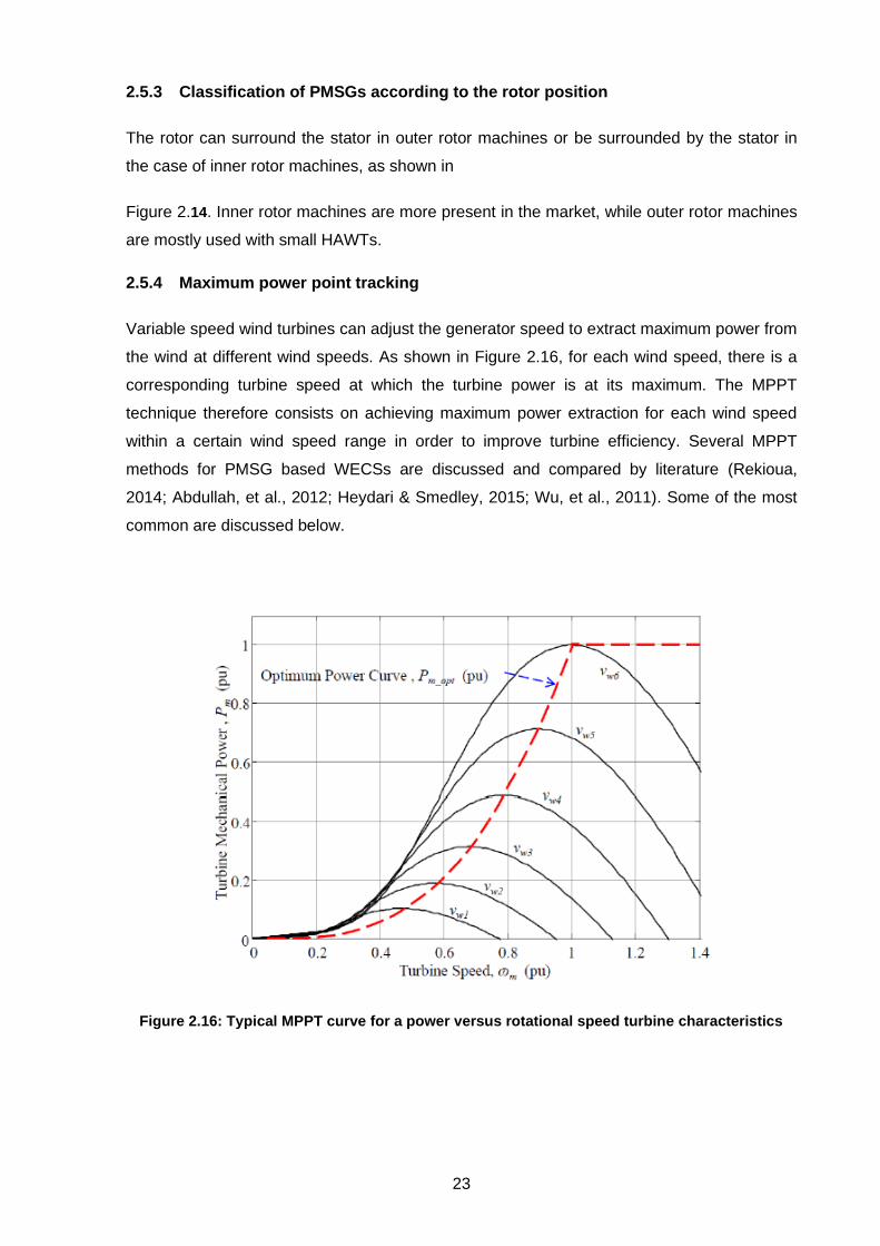
2.5.4 Maximum power point tracking
Variable speed wind turbines can adjust the generator speed to extract maximum power from
the wind at different wind speeds. As shown in Figure 2.16, for each wind speed, there is a
corresponding turbine speed at which the turbine power is at its maximum. The MPPT
technique therefore consists on achieving maximum power extraction for each wind speed
within a certain wind speed range in order to improve turbine efficiency. Several MPPT
methods for PMSG based WECSs are discussed and compared by literature (Rekioua,
2014; Abdullah, et al., 2012; Heydari & Smedley, 2015; Wu, et al., 2011). Some of the most
common are discussed below.
Figure 2.16: Typical MPPT curve for a power versus rotational speed turbine characteristics

24
PMSG
VECTOR
CONTROL
LOOKUP
TABLE
+
-
VDC
Turbine power
Ptur
ωr
ωr*
+-
Generator side
rectifier
Figure 2.17: PSF method applied to a PMSG based WECS
PMSG
VECTOR
CONTROLλOpt / R
+
-
VDC
Vwind
ωr
ωr*
+-
Generator side
rectifier
Figure 2.18: Optimal TSR method applied to a PMSG based WECS
2.5.4.1 Power signal feedback
This method uses a power versus wind speed curve to generate the reference turbine power
which is compared to the actual power at measured wind speed. The error signal is
compensated, and the actual power value will eventually equal the reference power at steady
state. The power signal feedback method is illustrated in Figure 2.17. To express the
maximum power-wind speed relationship, the following equation is used (Rekioua, 2014):
32
max 842.0125.008.13.0 VVVPm +−+−=− Equation 2.11
25
PMSG
VECTOR
CONTROLKopt.ωr
2
+
-
VDC
ωr
Generator side
rectifier
Topt
Figure 2.19: OTC method applied to a PMSG based WECS
PMSG
VECTOR
CONTROLP&O
Algrorithm
+
-
VDC
P[k]ωr*[k+1]
+-
Generator side
rectifier
ω[k]
P[k-1]
ω[k-1]
ωr*[k-1]
Figure 2.20: P & O method applied to a PMSG based WECS
2.5.4.2 Optimal tip speed ratio
From equation 2.10, it can be seen that the turbine power is a function of the tip speed ratio
(TSR) λ, and the pitch angle β. Equation 2.9 also shows that the value of λ depends on the
turbine speed ω and the wind speed V. Therefore, MPPT can be achieved by keeping the
TSR at its optimal value such that the turbine speed and power are maximum at different
wind speeds. This task can be completed in two different ways:
• Reference turbine speed is computed using measured wind speed and the optimal TSR.
This reference speed is then compared to the actual speed which is then corrected, and
the turbine operates at its MPP.
• The reference TSR is compared with its actual value, and the error signal is used to
generate the reference turbine power.

26
The optimal tip speed ratio is illustrated in Figure 2.18.
2.5.4.3 Optimal torque control
In OTC reference torque is generated using the torque-speed quadratic relationship from the
turbine power curve. OTC is illustrated in Figure 2.19. The maximum power coefficient Cpmax
and the optimal TSR λopt must be known. The relationship between the torque and the speed
can be expressed as (Heydari & Smedley, 2015):
2
optoptrefe kT =− Equation 2.12
where
3
max
55.0
opt
p
opt
Crk
=
Equation 2.13
2.5.4.4 Perturbation and observation (P & O) or Hill-climb searching (HCS)
As opposed to the other MPPT techniques mentioned above, The P & O is one method that
does not require any information about the turbine power curve or the wind speed. Instead,
an algorithm based on the principle of Hill-climb is used to determine and the track the
maximum operating point of the turbine’s power curve as shown in Figure 2.20. A change in
output power is first detected after a speed perturbation, then depending on the variation on
the output power, the next speed perturbation is programmed. The P & O method is further
elaborated in literature (Heydari & Smedley, 2015).
2.6 Power converters topologies for PMSG wind turbines
PECs play an important role in the performance of modern WTSs (Blaabjerg, et al., 2009).
The PECs can be grid connected or standalone as used in most remote areas without grid
interconnection (Prerna & Jagdeesh Kumar, 2013), unidirectional or bidirectional depending
on the power flow (Khater & Omar, 2013), two-level or multilevel (Blaabjerg, et al., 2009).
Power converters for WECS are widely discussed by many references (Yamarasu, et al.,
2015; Wu, et al., 2011).
2.6.1 Thyristor grid-side inverter
The grid-side inverter uses thyristors to control the inverter’s firing angle. This way the
turbine speed is regulated through the DC link voltage, allowing maximum energy to be
captured. The main advantage of this configuration is that it has a low cost for a high-power
rating. However, there is a need for reactive power compensation, as well as total harmonic
distortion reduction. Therefore, an active compensator filter is used, with a voltage source
converter (VSC) as shown in Figure 2.21a. The Pulse width modulated (PWM) control is
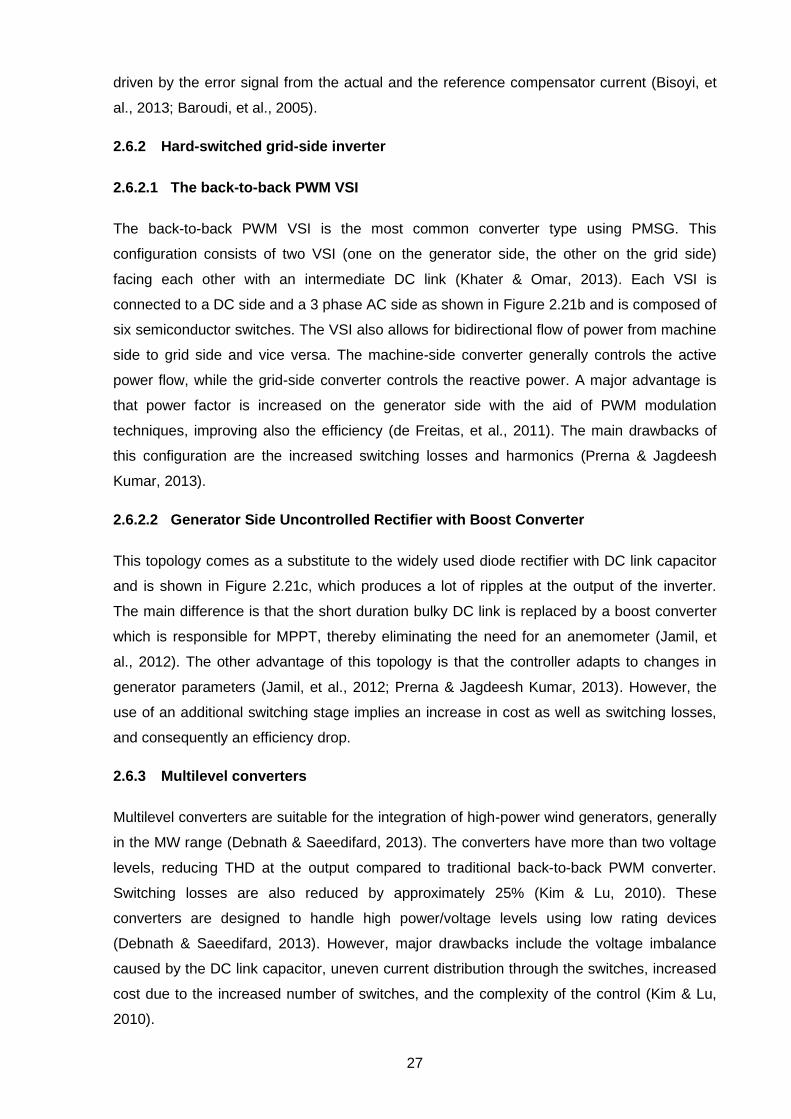
27
driven by the error signal from the actual and the reference compensator current (Bisoyi, et
al., 2013; Baroudi, et al., 2005).
2.6.2 Hard-switched grid-side inverter
2.6.2.1 The back-to-back PWM VSI
The back-to-back PWM VSI is the most common converter type using PMSG. This
configuration consists of two VSI (one on the generator side, the other on the grid side)
facing each other with an intermediate DC link (Khater & Omar, 2013). Each VSI is
connected to a DC side and a 3 phase AC side as shown in Figure 2.21b and is composed of
six semiconductor switches. The VSI also allows for bidirectional flow of power from machine
side to grid side and vice versa. The machine-side converter generally controls the active
power flow, while the grid-side converter controls the reactive power. A major advantage is
that power factor is increased on the generator side with the aid of PWM modulation
techniques, improving also the efficiency (de Freitas, et al., 2011). The main drawbacks of
this configuration are the increased switching losses and harmonics (Prerna & Jagdeesh
Kumar, 2013).
2.6.2.2 Generator Side Uncontrolled Rectifier with Boost Converter
This topology comes as a substitute to the widely used diode rectifier with DC link capacitor
and is shown in Figure 2.21c, which produces a lot of ripples at the output of the inverter.
The main difference is that the short duration bulky DC link is replaced by a boost converter
which is responsible for MPPT, thereby eliminating the need for an anemometer (Jamil, et
al., 2012). The other advantage of this topology is that the controller adapts to changes in
generator parameters (Jamil, et al., 2012; Prerna & Jagdeesh Kumar, 2013). However, the
use of an additional switching stage implies an increase in cost as well as switching losses,
and consequently an efficiency drop.
2.6.3 Multilevel converters
Multilevel converters are suitable for the integration of high-power wind generators, generally
in the MW range (Debnath & Saeedifard, 2013). The converters have more than two voltage
levels, reducing THD at the output compared to traditional back-to-back PWM converter.
Switching losses are also reduced by approximately 25% (Kim & Lu, 2010). These
converters are designed to handle high power/voltage levels using low rating devices
(Debnath & Saeedifard, 2013). However, major drawbacks include the voltage imbalance
caused by the DC link capacitor, uneven current distribution through the switches, increased
cost due to the increased number of switches, and the complexity of the control (Kim & Lu,
2010).

28
PMSG
Diode
rectifier SCR inverter
Compensator
a) PEC with SCR inverter
PMSG
Grid-side
inverter
Machine-side
rectifier
b) PEC using back-to-back hard switch configuration
PMSGBoost
converter
Diode
rectifier
Hard-
switched
grid-side
inverter
c) Typical PEC using diode rectifier and intermediate boost converter
Figure 2.21: Examples of PECs used with PMSG based WECS
There are many multilevel converter topologies at this day (Kim & Lu, 2010), the most
common being the neutral point clamped (NPC), the cascaded half-bridge (CHB), and the
flying capacitors (FC). Of them all, the NPC is still the most appreciated and widely used
(Kim & Lu, 2010).
2.6.4 Matrix converters
The matrix converter (MC) is a particular design that eliminates the DC stage from the
traditional AC-DC-AC conversion process, to the profit of a direct AC-AC conversion. This
arrangement has the advantage that the bulky DC link capacitors and/or inductors are
inexistent, and so are the associated lifetime, size, and cost issues. The output voltage

29
magnitude, frequency, phase angle, as well as the input power factor are controlled
independently, due to the large number of control levels that the MC provides. However, the
main disadvantages of the MC are its complex control due to commutation problems, the
scarcity of monolithic bi-directional switches, the lack of decoupling between the two AC
sides of the converter, and the low voltage gain (Pandu Ranga & Vijaya, 2013; Yang & Li,
2009).
2.6.5 Z-source converters
Also called impedance source converters, z-source converters have been designed to
overcome operating range limitations of both voltage source converters and current source
converters. They use an X shaped impedance network to connect machine and grid side
converters. They are widely discussed in literature(Peng, 2002; Vilathgamuwa, et al., 2008;
Florescu, et al., 2010).
2.7 Power converter control
The control system, just as much as the hardware, plays an important role in the overall
performance of a wind turbine system. The controller is designed for the wind turbine to
reach specific objectives that can be summarized as follows (Soriano, et al., 2013):
· Extract maximum power from the wind
· Ensure maximum output power for different wind speeds
· Deliver quality power according to network provider standards
· Comply with grid interconnection requirements
· Reduce stress on mechanical components during turbulences
According to many references (Busca, et al., 2010; Quang & Dittrich, 2008; Allagui, et al.,
2014; Jash, et al., 2013), vector control is the most popular and most widely used method for
the control of PEC in a WTS. Comparisons of different vector control techniques were done
by different authors with emphasis on the FOC (Field Oriented Control) and DTC (Direct
Torque Control) on the generator side (Busca, et al., 2010; Allagui, et al., 2014; Huang,
2013), and VOC (Voltage Oriented Control) and DPC (Direct Power Control) on the grid side
(Huang, 2013; Allagui, et al., 2014).
The FOC technique seems to be more attracting than the DTC for direct-drive applications
since it presents a good performance at relatively low speeds, offers quick speed and torque
responses, as well as reduced torque ripples and minimal power-tracking error. On the other
hand, DTC is easier to implement than FOC and offers fast transient response, but presents
drawbacks such as difficulties in torque control, increased ripples and noise level, which are
even more pronounced at very low speeds. On the grid side, both strategies present similar

30
results and they both meet grid code requirements. However, VOC presents lower THD and
higher efficiency while DPC provides a better dynamic response.
As far as modulation techniques are concerned, space vector modulation (SVM) techniques
are mostly employed (Freire, 2013). Other techniques use a carrier signal that is compared
to a reference modulation signal, or hysteresis current control (Wu, et al., 2011; Zeng &
Chang, 2005). Comparisons of some of these techniques shows that SVM applied with pulse
width modulation present a better steady state performance under normal operations or
during grid faults, while HCC presents better results for faults on the generator side (Freire,
2013). When SVM is used with DTC, the results are similar to the FOC technique (Busca, et
al., 2010).
2.8 Summary of the chapter:
In this section, an overview of already available and most common wind turbine technologies
was presented. The fundamentals of a wind energy conversion system were first discussed,
including the different components of a wind turbine, as well as its aerodynamics principles
and the different maximum power extraction methods. The different generator, power
electronics converters, and drive train topologies of the main wind turbine concepts from
fixed speed to variable speed were also discussed and compared. The direct driven PMSG
full scale variable speed topology was proven to be a better option compared to other
concepts due to many reasons such as an increased generator efficiency, the absence of
gearbox, and more flexible controllability due to the bidirectional nature of the converters.
Finally, the different PECs and control techniques were also discussed and compared.

31
CHAPTER THREE
3 GRID CODE REQUIREMENTS AND LVRT SOLUTIONS
Introduction
Grid codes are important to ensure a safe and reliable transmission of electric power within
the interconnected network. They represent a guideline defined by each transmission system
operator (TSO) to which each power producer must adhere in order to be connected to the
grid. In South Africa, electric power is generated from various sources including coal, gas,
water, and renewables. In this chapter, a review the grid code requirements for wind power
plants connected to the electric power network is presented and the case of South Africa is
analysed in more details. Low voltage ride-through being the core of this research, a review
of the different LVRT solutions for a PMSG based wind energy conversion system is also
presented.
3.1 Grid code requirements for wind farms
Grid power quality and network stability are major challenges issued from the massive
integration of large-scale high-power wind turbines into the grid. As such, wind turbine
operators have developed new grid code requirements that WTSs and WPPs need to satisfy
when connected to the network. These important requirements are usually classified into four
categories namely active power control, reactive power and voltage control, frequency and
voltage operating range, and fault ride-through capability with following objectives:
(Sourkounis & Tourou, 2013)
• Control the active power supplied to the grid during frequency and voltage disturbances
• Define appropriate ranges of frequency and voltage and ensure WPPs operation within
the specified limits
• Contribute to the grid power balance by injecting or absorbing reactive power.
• Support voltage recovery at connection point after fault occurrence
• Maintain smooth connection to the network in the event of small duration voltage dips
Because transmission systems differ due to different standards, most grid code requirements
also present different tolerance, limitation and operating values. Grid code requirements of
many countries are reviewed and compared in literature (Tsili, et al., 2009; Mohseni & Islam,
2011).

32
Figure 3.1: Voltage and frequency operating ranges as defined by German power system
operator (Mohseni & Islam, 2012)
Figure 3.2: Frequency operating limits in some of the European countries

33
(a) Absolute power constraint
(b) Delta production constraint
(c) Balanced regulation
(d) Power gradient constraint
Figure 3.3: Active power regulation strategies (de Alegria, et al., 2007)
3.1.1 Frequency and voltage operating range
Many grid codes have voltage and frequency variation ranges or limits within which wind
farms are expected to carry on a smooth and continuous operation even during small
disturbances (Sourkounis & Tourou, 2013; Tsili, et al., 2009). Past these limits specified by
system operators, system stability is no longer guaranteed, and wind farms and the rest of

34
the power system may be endangered. In this case, disconnection of WPPs seems to be the
most appropriate option.
A graphical representation of voltage and frequency operating ranges as defined by general
grid codes is illustrated in Figure 3.1. Generally, WPPs operate continuously at frequencies
equal to or very close to the nominal value and do only operate for minor time durations
when frequencies exceed certain values as illustrated in Figure 3.2.
3.1.2 Active power control
Large positive or negative differences between actual and nominal frequency values usually
indicate a power system imbalance. Frequency changes could be caused either by a fault on
the network, or by acute wind speed variations. In response to these instabilities and to
reinstate close to nominal frequency, grid codes require that WPPs have the capability to
provide network frequency supports through the control of their generated active power.
WPPs should be capable of reducing or regulating their output power to a predefined
magnitude, whenever requested from the system operator. This may be achieved by
minimizing the extracted wind power using a pitch angle control on the turbine blades in as
explained earlier in section 2.3.3 (Sourkounis & Tourou, 2013; Tsili, et al., 2009). Figure 3.1
shows a typical curve of output power variation in response to frequency changes. The curve
shows that the output power will gradually decrease as the frequency increases above
nominal value. It is important to note that the output power delivered is slightly lower than the
maximum achievable level. This is to allow the output power to increase up to its maximum
value, such that the frequency can be sustained when its value falls below nominal value (de
Alegria, et al., 2007).
It is also important that active power be reduced or restored at a satisfactory rate when a
voltage dip occurs or is cleared, to avoid generator over-speeding or power surges which
could result in damage of wind generator and power system disturbances. Active power
production is managed using different strategies in order to fulfil all of the above-mentioned
frequency and voltage requirements. Some of the most common are listed below and
presented in Figure 3.1 (Mohseni & Islam, 2012):
• The active power can be controlled so that its value can never exceed a pre-set
maximum value regardless of whether more wind power is available or not. This
regulation mode is known as active power constraint. Generally, when wind power
production is greater than the demand, wind turbine operators usually lose money since
they are required to pay for excess production.

35
• The power output is maintained at a slightly lower level to allow frequency control as
explained above and achieve delta production constraint.
• The active power supplied to the grid is controlled such that it can be quickly reduced on
fault occurrence or increased at fault clearance to ensure balanced power production
and consumption. This control is therefore named balanced regulation.
• The power gradient constraint is used to regulate the rate at which WPP power is
supplied to the grid to the level of conventional power plants by setting a maximum
gradient that cannot be exceeded.
3.1.3 Reactive power and voltage control
The purpose of the reactive power and voltage control requirement is to ensure that system
operation under required limits is properly achieved, reducing risks of network instabilities.
Wind farms should have reactive power control capability for the purpose of supporting the
voltage at the PCC (point of common coupling), as well as the reactive power demand from
the grid (Sourkounis & Tourou, 2013). This means that WPPs should be able to supply
lagging or leading reactive power depending on whether power is supplied to or absorbed
from the PCC, while keeping the power factor within an acceptable range as illustrated in
Figure 3.6. In some grid codes, the network operator should set a particular reference value
for the reactive power at the wind farm connection point (Tsili, et al., 2009). Figure 3.6 shows
the graphs of the requirement of reactive power variation with respect to changes in voltage
for the case of Germany (Mohseni & Islam, 2012; de Alegria, et al., 2007).
3.1.4 Low Voltage Ride Through capability
New grid codes specifications require that wind farms be able to survive voltage faults up to
a certain percentage of the nominal voltage, and for a precise time interval, while remaining
coupled to the power system. In addition, active and reactive power should quickly ramp
back to nominal value after fault clearance. This requirement is essential for a smooth and
continuous supply from the power system by avoiding possible disconnection which could
lead to further losses of generation capacity, and eventual collapse of the network
(Sourkounis & Tourou, 2013; Tsili, et al., 2009).
The LVRT requirement is expressed using a voltage vs time characteristic curve which
delineates the region under which the wind turbine should safely operate in the event of a
grid fault (Leao, et al., 2010). An example of such curve is shown in Figure 3.6. Wind
turbines should remain connected as long as the voltage at point of common coupling (PCC)
is above delineated region, otherwise disconnection is allowed.
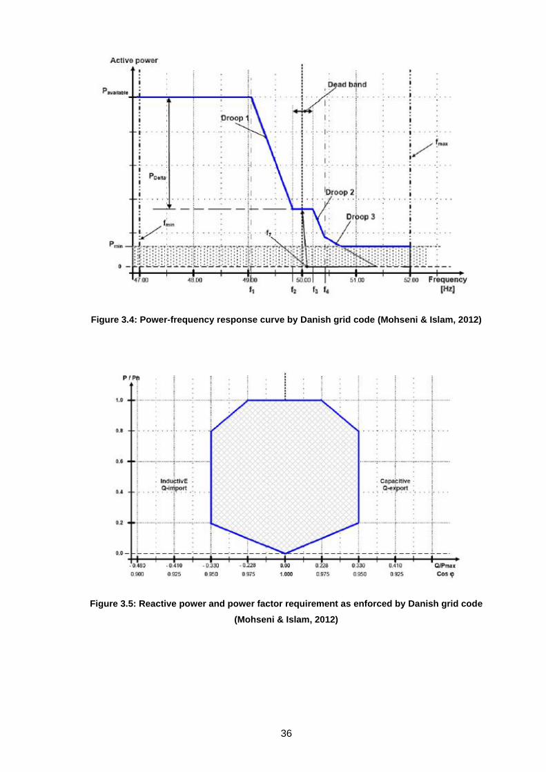
36
Figure 3.4: Power-frequency response curve by Danish grid code (Mohseni & Islam, 2012)
Figure 3.5: Reactive power and power factor requirement as enforced by Danish grid code
(Mohseni & Islam, 2012)
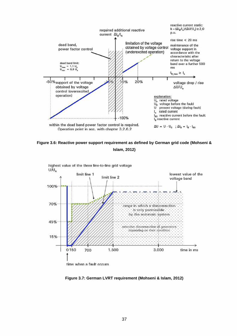
37
Figure 3.6: Reactive power support requirement as defined by German grid code (Mohseni &
Islam, 2012)
Figure 3.7: German LVRT requirement (Mohseni & Islam, 2012)

38
Figure 3.8: South African LVRT curve (Mchunu & Khoza, 2013)
Figure 3.9: Requirement for reactive power support during grid fault according to the South
African grid code (Mchunu & Khoza, 2013)

39
Table 3.1: Classification of RPPs according their rated power (Mchunu & Khoza, 2013)
Sub-categories Rated power range (kVA)
A1 0 < A1 ≤ 13.8 kVA
A2 13.8 kVA < A2 < 100 kVA
A3 100 kVA ≤ A3 <1MVA
B 1 MVA ≤ B < 20 MVA
C ≥ 20 MVA
For a wind turbine to successfully achieve the FRT, grid code requirements as well as wind
turbine requirements should be met whenever a fault occurs in the grid. Therefore, on the
grid side, wind turbines should be able to remain connected according to the FRT curve,
supply reactive power to the grid, and recover active power. On the generator side, excess
current and voltage on the stator or rotor, torque ripples, changes in turbine’s speed,
overvoltage on the dc-link should be avoided (Hu, et al., 2010).
3.1.5 South African grid code requirements for Renewable Power Plants
The South African grid code for renewable power plants (RPPs) was established by the
National Energy Regulator of South Africa (NERSA) aiming for reliability, safety and security
of the interconnected power system. This code ensures that RPPs connected or still to be
connected to the power network meet specific technical and design requirements (Mchunu &
Khoza, 2013). These requirements are defined according to different categories from A to C,
depending on the power rating of the RPP as specified in Table 3.1.
With the South African grid code for RPPs, the same requirements listed earlier are also
applicable. RPPs should be capable of operating within a certain limit of frequencies and
voltages as well as contributing to network stability under faulty circumstances. The South
African grid code requirements are presented by Mchunu & Khoza (2013). However, only the
LVRT requirement is covered.
During voltage sags arising from symmetrical or unsymmetrical faults, RPPs should remain
connected to the grid as shown in Figure 3.8. The FRT curve is divided into 4 sections each
representing different operating regions for the RPPs.
• Area A: continuous operating region where the RPP should maintain normal production.
This region is comprised between 0.9 and 1.1 pu, approximately ±10% of the rated
voltage at the POC.
• Area B: faulty region for which the RPP is required to remain stable and connected to
the network. In this operating mode, active power must be maintained for voltage drops
up to 85% of rated value, otherwise reduction is required proportionally to the voltage

40
drop. The reduced active power is expected to recover within 1 second to at least 90%
of pre-fault value. Voltage drops up to zero should be tolerated for maximum fault
clearance duration of 150 millisecond. Moreover, the RPP should contribute to voltage
stabilization by injecting reactive power as illustrated in Figure 3.9.
• Area C: the RPP may be disconnected from the network.
• Area D: the nominal voltage at POC can reach peaks of up to 120% without
disconnection of the RPP for duration not exceeding 2 seconds. This area is only
applicable to RPPs of category C.
3.2 LVRT methods for PMSG WTs
In a full-scale variable speed WT, the generator side and the grid side are decoupled by the
PEC. During a fault at the PCC, the terminal voltage is considerably reduced, which implies
that the active power supplied to the grid is also reduced. On the other side, the generator
keeps on supplying power since not directly connected to the grid. This excess power is
stored in the dc-link and will later lead to dc-link over-voltage and voltage oscillation which
could affect steady state operation of the generator and cause damages to the converter and
the WTS (Dong, et al., 2012). In order to avoid this situation, a number of techniques have
been proposed by different references.
Nasiri et al (2015) present a review and comparison of some of the most popular LVRT
techniques used with PMSG WECSs. The paper classifies these techniques into two
categories depending on whether additional devices are used or not in order to achieve
LVRT as presented in figure 3.10. In the second case, the LVRT is achieved by simply
modifying control strategy, without the need for external action. These techniques are
referred to as “modified control-based methods”. Some of the most used LVRT techniques
are discussed below.
3.2.1 Modified control-based techniques
3.2.1.1 Change of control strategy
The control of the DC-link voltage is achieved by the MSC, while the active and reactive
power control task is done by the GSC, as opposed to the traditional control in which the
GSC is responsible for DC-link voltage control and active power is controlled on the machine
side. In this method, the DC-link voltage regulation is accomplished by decreasing the
generator stator current and thus the power flow to the DC-link. The excess energy is
converted to rotational energy, increasing the turbine’s rotational speed which is directly pitch
controlled if the speed exceeds the rated value. An external damping controller is also used
in this system (Hansen & Michalke, 2009).

41
LVRT Solutions
Additional devices Modified control
Braking
chopperESS
Capacitor
sizingFACTS BPA
Change of control
strategy
Figure 3.10: LVRT enhancement techniques
Desired pitch angleInput variables
Pitch actuatorPitch angle reference
computation+_
Figure 3.11: Block diagram of a typical BPA controller
3.2.1.2 Blade pitch angle (BPA) control
Apart from being used for maximum wind energy extraction at low wind speeds or for
minimum extraction at more than rated wind speeds, BPA control is also used for LVRT
(Conroy & Watson, 2007; Yang, et al., 2009). In this case, the aim of the pitch controller is to
reduce the energy captured by the turbine blades during a grid fault, by pitching out of the
direction of the wind. This technique is simple and cheap but offers a slow response due to
its mechanical nature. Therefore, the BPA control is usually used in addition to other fast
LVRT techniques to improve the system’s response.
BPA control techniques are usually closed loop systems where the actual measured pitch
angle is compared to a reference value which can be controlled either from wind speed,
generator speed or torque, and power measurements (Ben Smida & Sakly, 2015) as
illustrated in figure 1. In Conroy & Watson (2007), during a grid fault condition, the controller
switches from the normal operating mode to an emergency mode and the reference pitch
angle is specified by its emergency value. For Nasiri, et al., (2015), the control in figure 3.11
above is used when wind speeds exceed nominal value, while grid voltage differences are
used to generate the reference pitch angle in the event of a fault (Nasiri, et al., 2015).

42
3.2.2 Additional devices-based techniques
3.2.2.1 Capacitor sizing
Storing the excess energy from the generator into another capacitor of larger size is an
alternative way of decreasing the energy to be absorbed by the dc-link capacitor during a
voltage dip. Since the required capacitor power increases with the duration of the voltage dip,
longer voltage dips will imply larger capacitor sizes. Capacitor sizing is therefore an
inappropriate method and is usually not used (Conroy & Watson, 2007).
3.2.2.2 Braking resistor (DC chopper)
A DC chopper circuit which consists of a braking resistor controlled by a switch is connected
in parallel with the DC-link capacitor as shown in Figure 3.12. Whenever the dc-link voltage
exceeds a predefined value, the switch is activated and the excess energy is dissipated
through the resistor (Rosyadi, et al., 2011). This method can also be combined to the pitch
control technique for a more effective result especially for longer voltage dips, reducing the
rating of the protective resistor and thus the overall cost (Ibrahim, et al., 2012).
Qiu, et al., (2011) and Kesraoui, et al., (2010) used a bypass chopper with the diode rectifier
configuration to dissipate the excess power. The error signal from the DC-link voltage
reference and measured values is sent through a PI regulator to control the duty cycle of the
switch. For Shuju, et al., (2008) the generated power, the grid power and the DC-link voltage
measurements are used to determine the state of the switch and to calculate its duty cycle.
For Yan, et al., (2011), a signal is sent to the controller at the occurrence of a grid fault, and
the IGBT switch is directly triggered and remains on until fault clearance. Heng, et al., (2008)
used a D flip-flop to generate the switching command to the switch. A predefined threshold
value is compared to the actual DC-link value using a comparator circuit. The input to the flip-
flop is the output from the comparator.
3.2.2.3 Energy storage system
An Energy storage system (ESS) is also used to store the excess energy from the generator
or to supply power to the grid if necessary (Nguyen & Lee, 2010). This method also improves
power quality on the grid by charging or discharging the fluctuating power component that
derives from changes in wind speed. Lead acid batteries (LAB), sodium sulphur batteries
(SSB), and vanadium redox flow batteries are mostly used due to their lifespan, their storage
capacity, low cost and quick dynamic response. However, an additional dc-dc converter is
required in order to regulate the excess voltage to the battery rating (Ibrahim, et al., 2012;
Nasiri, et al., 2015). A typical WECS equipped with an ESS is shown in Figure 3.12.
43
PMSG
AC/DC DC/AC Grid
Braking chopper
Figure 3.12: Braking chopper configuration
PMSG
ESS
AC/DC DC/AC Grid
Figure 3.13: Energy storage system connected to the DC-link
PMSG
AC/DC DC/AC Grid
STATCOM
Figure 3.14: Typical structure of a STATCOM

44
PMSG
AC/DC DC/ACGrid
DVR
Figure 3.15: Typical configuration of a dynamic voltage restorer
PMSG
AC/DC DC/ACGrid
UPFC
Figure 3.16: Typical configuration of a unified power flow controller
3.2.2.4 The use of FACTS devices
Facts (Flexible AC transmission systems) devices have the advantage that they can supply
reactive power to the grid. They can be connected in parallel (shunt connection), series
(series connection), or in a combination of series and parallel (Hybrid connection) with the
common coupling point. In shunt connection, the amount of reactive power injected on the
grid depends on the reactive power demand from the grid during a grid fault, as well as the
reactive power transfer capability from the wind farm. The two main shunt compensation
devices are the Static Synchronous Compensator (STATCOM) and the Static VAR
compensator (SVC). Although these techniques are mostly used with DFIGs, they can also
be used with PMSG based wind turbines (Chowdhury, et al., 2012; Nguyen & Lee, 2013).
The basic configurations of STATCOM is shown in Figure 3.12.
Series connection devices inject capacitive voltage at the PCC to increase the reactive
power supply from the grid. These devices include the thyristor-controlled series capacitor

45
(TCSC), Static Synchronous Series Compensator (SSSC), the Dynamic Voltage Restorer
(DVR), the Magnetic Energy Recovery Switch (MERS), and more (Wenming, et al., 2011;
Ibrahim, et al., 2012). The configuration of a DVR is shown in Figure 3.12.
As for the hybrid connection, the Unified power flow controller (UPFC) is the state-of-the-art
of this technology. UPFCs have the advantage that they can inject capacitive voltage for
voltage recovery from the series connection, as well as reactive power for grid support from
the shunt connection (Raphael & Massoud, 2011). The UPFC is typically a back-to-back
connection of STATCOM and SSSC as illustrated in Figure 3.12.
Summary of the chapter
This chapter presented an overview of the existing grid code requirements to be met for
WPPs to be connected to transmission and distribution networks in some developed
countries. Frequency and voltage range, active power control, reactive power and voltage
control, and FRT capability were depicted as the most commonly used by many grid
operators. These requirements were detailed and explained thoroughly. The case of FRT
and particularly the LVRT of the South African grid code was more deeply examined.
An overview of LVRT enhancement solutions was also presented in this chapter. These
solutions were categorised into two depending on whether additional components were
needed or not. The advantages and disadvantages were presented, and the solutions were
compared.

46
CHAPTER FOUR
4 WIND TURBINE SYSTEM MODELING
Introduction
Before carrying out any simulation studies on the WECS, a detailed model of the different
components that constitute the system needs to be implemented. This chapter discusses the
mathematical modeling of the full scale variable speed WECS including all controllers. The
WECS consists of a direct-driven PMSG wind turbine connected to the grid through a back-
to-back converter. The advantages and drawbacks of this configuration are already
presented in section 2.4. A WECS equipped with PMSG and full scale power converter is
represented in
Figure 1.1. As illustrated, the WTS is composed of a mechanical part which converts the
energy from the wind into mechanical rotational energy through the turbine blades and the
drive train, as well as an electrical part (PMSG, PEC, filters, transformers) which converts the
mechanical energy from the drive train to quality electrical power to be fed into the grid
(Kasem Alaboudy, et al., 2013).
To accurately emulate the dynamic behaviour of the wind turbine and its impacts when
connected to a power system, different key components such as the turbine and mechanical
shaft dynamics, generator electrical and mechanical characteristics, power converter
controls, protection settings and measurements of critical variables, need to be taken into
consideration in the mathematical model for time domain simulations (Vittal & Ayyanar,
2013).
4.1 Wind turbine model
The power extracted by the turbine was expressed in Equation 2.10 of chapter 2. The power
coefficient Cp (λ, β) was modelled using the following equation (Heir, 2014):
0068.0)54.0/116.(5176.0),(
/21+−−=
− ieC ip Equation 4.1
with
Equation 4.2
Figure 4.2 represents typical Cp (λ, β) characteristics for different pitch angles and tip speed
ratios. It can be observed that maximum power coefficient occurs at pitch angle β=0 degrees.
This value also corresponds to the nominal tip speed ratio.
1
035.0
08.0
113 +
−+
=i

47
PMSG
AC
ACDC
DCDrive
trainFilter Grid
Control SystemPitch angle β
Rotor speed ωm
Stator voltage and
current, Vs and Is
Grid voltage and
current, Vgrid and Igrid
DC link
voltage
Wind
speed
VDC
Stator
reference
active power
Grid
reference
reactive
power
Vwind Pref Qref
Turbine
speed ωt
Reference voltages
Figure 4.1: PMSG based wind turbine system
Figure 4.2: Power coefficient as a function of tip speed ratio (Perelmuter, 2013)
4.2 Drive train model
Different mechanical parts constitute the drive train of a wind turbine. These parts include the
rotor, the shaft, the gearbox, and generator. The complexity of the drive train usually
depends on the objectives and requirements of the study. Therefore, a one-mass, two-mass,
or three-mass model may be used as the number of parameters to be considered increases.
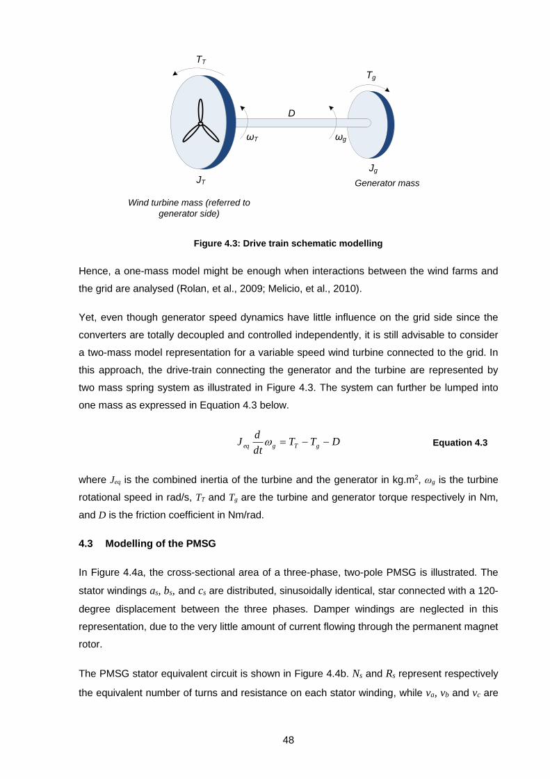
48
JT
Jg
ωg
D
Tg
TT
ωT
Wind turbine mass (referred to
generator side)
Generator mass
Figure 4.3: Drive train schematic modelling
Hence, a one-mass model might be enough when interactions between the wind farms and
the grid are analysed (Rolan, et al., 2009; Melicio, et al., 2010).
Yet, even though generator speed dynamics have little influence on the grid side since the
converters are totally decoupled and controlled independently, it is still advisable to consider
a two-mass model representation for a variable speed wind turbine connected to the grid. In
this approach, the drive-train connecting the generator and the turbine are represented by
two mass spring system as illustrated in Figure 4.3. The system can further be lumped into
one mass as expressed in Equation 4.3 below.
DTTdt
dJ gTgeq −−= Equation 4.3
where Jeq is the combined inertia of the turbine and the generator in kg.m2, ωg is the turbine
rotational speed in rad/s, TT and Tg are the turbine and generator torque respectively in Nm,
and D is the friction coefficient in Nm/rad.
4.3 Modelling of the PMSG
In Figure 4.4a, the cross-sectional area of a three-phase, two-pole PMSG is illustrated. The
stator windings as, bs, and cs are distributed, sinusoidally identical, star connected with a 120-
degree displacement between the three phases. Damper windings are neglected in this
representation, due to the very little amount of current flowing through the permanent magnet
rotor.
The PMSG stator equivalent circuit is shown in Figure 4.4b. Ns and Rs represent respectively
the equivalent number of turns and resistance on each stator winding, while va, vb and vc are

49
the stator phase terminal voltages. Figure 4.4c shows the per phase equivalent circuit of the
PMSG.
a-axis
q-axis
b-axis
c-axis d-axis
a’
cb
a
b’c’θr
N
S
(a) Cross sectional view of a two-pole PMSG
Rs
Rs
Rs
Ls
Ls
Ls
ib
ia
ic
vb
va
vc
(b) Three-phase equivalent circuit of a PMSG
Rs jXsIs
N SVs
+
_
Ef
(c) Per phase equivalent circuit of a PMSG
Figure 4.4: Representation of a 2-pole, 3-phase, star connected PMSG

50
φs
δ
Ef
Vs
Is
IsRs
I sjX s
IsZsφs
Figure 4.5: Phasor diagram of a PMSG
From Figure 4.4c, the phasor diagram of the PMSG is derived as illustrated in Figure 4.5
above, with the assumption that the current lags the voltage by a certain angle φs. This angle
serves to determine the generator active and reactive powers Ps and Qs expressed as:
ssss
ssss
IVQ
IVP
sin3
cos3
=
= Equation 4.4
The following relation can be derived from Figure 4.5:
sincoscossins
f
sssssfZ
EIIZE == Equation 4.5
where δ, known as power angle, is the angle between Ef and Vs. Therefore, the generator
active power can be rewritten as:
sin3s
fs
sZ
EVP = Equation 4.6
Also, from Figure 4.5, the following relation can be obtained:
s
sf
ssssssfZ
VEIIZVE
−=+=
cossinsincos Equation 4.7
In the same manner as the active power, the reactive power can be rewritten as:
s
sf
sZ
VEQ
−=
cos3 Equation 4.8

51
Since Rs<<Xs, Equation 4.6 and Equation 4.8 can be rewritten neglecting Rs as:
s
sf
s
s
fs
s
X
VEQ
X
EVP
−=
=
cos3
sin3
Equation 4.9
When developing the model of a PMSG, it is assumed that (Kundur, 1994):
· The induced emf is sinusoidal
· The field current remains constant
· Magnetic hysteresis and eddy currents are negligible
· Magnetic saturation effects are negligible
· Permanent magnets have no conductivity
4.3.1 Reference frame theory
In order to simplify the analysis of synchronous and induction machines, as well as the
implementation of different WECS based control techniques, reference frame
transformations from natural three-phase abc to two-phase stationary αβ and rotating dq
synchronous frames and vice-versa, are often utilised. The abc to αβ transformation also
known as Clark’s transformation is given as (Wu, et al., 2011):
Equation 4.10
Similarly, the inverse Clark’s from αβ to abc is given by:
−−
−=
x
x
x
x
x
c
b
a
2/32/1
2/32/1
01
Equation 4.11
Park’s transformation is used to switch from the natural abc frame to the dq frame. The
Park’s transformation and inverse Park are given by Equation 4.12 and Equation 4.13
respectively:
−−−−−
−−=
c
b
a
q
d
x
x
x
x
x.
)3/4sin()3/2sin(sin
)3/4cos()3/2cos(cos
3
2
Equation 4.12
−
−−=
c
b
a
x
x
x
x
x.
2/32/30
2/12/11
3
2

52
−−−
−−−
−
=
q
d
c
b
a
x
x
x
x
x
.
)3/4sin()3/4cos(
)3/2sin()3/2cos(
sincos
Equation 4.13
4.3.2 Dynamic model
The voltage equations of the PMSG in the d-q axis rotor field synchronous reference frame
can be expressed using the following equations (Wu, et al., 2011; Bunjongjit & Kumsuwan,
2013):
qsqsdsrqssqs
dsdsqsrdssds
dt
dLiRv
dt
dLiRv
+−−=
+−−=
Equation 4.14
where vds, vqs, ids, iqs, Ld, Lq, represent the d and q axis stator voltages, currents, and self-
inductances respectively. The d and q-axis stator flux linkages are given as:
qsqqs
rdsdds
iL
iL
−=
+−=
Equation 4.15
The rotor flux λr and the d and q-axis self-inductances Ld and Lq are in turn defined by:
qmlsq
dmlsd
fdmr
LLL
LLL
IL
+=
+=
=
Equation 4.16
where Ldm and Lqm represent the d and q axis magnetising inductances respectively, Lls
represents the stator leakage inductance, and If is the field current.
Substituting Equation 4.15 into Equation 4.14, the voltage equations can be rewritten as:
qsqsrrdsdsrqssqs
dsdsqsqsrdssds
idt
dLiLiRv
idt
dLiLiRv
−+−−=
−+−=
Equation 4.17
The electromagnetic torque is given by the formula:
( )qsdsdsqse iiP
T −=2
3 Equation 4.18
where P represents the number of pole pairs.

53
Substituting Equation 4.15 into Equation 4.18, the expression for electromagnetic torque can
be rewritten as:
( ) qsdsqdqsre iiLLiP
T -2
3−= Equation 4.19
Finally, the rotor speed is expressed as:
)( mer TTJS
P−= Equation 4.20
with Tm representing the mechanical, J the rotor inertia, and S the Laplace operator.
4.3.3 Steady state model
In the steady-state model, stator currents ids and iqs are considered DC values, making their
derivatives equal to zero. Equation 4.17 above becomes (Wu, et al., 2011):
rrdsdsrqssqs
qsqsrdssds
iLiRv
iLiRv
+−−=
+−=
Equation 4.21
4.3.4 Equivalent circuit of the PMSG
The simplified equivalent circuits of the PMSG are shown in Figure 4.6a and 4.6b for the
dynamic and steady state models respectively. Note that the direction of the currents is out of
the stator. This representation is according to the generator mode convention
vqs Lq
Rs ωrLdidsiqs ωrλr
_
+
vds Ld
Rs ωrLqiqsids
+
_
(a) Dynamic model
ids Rs ωrLqiqs
vds
_
+
Rs ωrLdidsiqs ωrλr
_
vqs
+
(b) Steady state model
Figure 4.6: Simplified equivalent circuits of PMSG
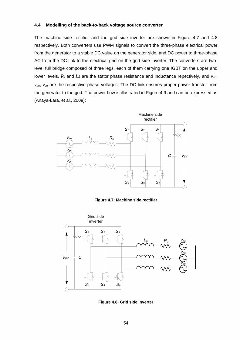
54
4.4 Modelling of the back-to-back voltage source converter
The machine side rectifier and the grid side inverter are shown in Figure 4.7 and 4.8
respectively. Both converters use PWM signals to convert the three-phase electrical power
from the generator to a stable DC value on the generator side, and DC power to three-phase
AC from the DC-link to the electrical grid on the grid side inverter. The converters are two-
level full bridge composed of three legs, each of them carrying one IGBT on the upper and
lower levels. Rs and Ls are the stator phase resistance and inductance repectively, and van,
vbn, vcn are the respective phase voltages. The DC link ensures proper power transfer from
the generator to the grid. The power flow is illustrated in Figure 4.9 and can be expressed as
(Anaya-Lara, et al., 2009):
Machine side
rectifier
VDC
RsLsvan
vbn
vcn
S1 S2 S3
S4 S5 S6
IDC
C
Figure 4.7: Machine side rectifier
VDC
RgLg van
S1 S2 S3
S4 S5 S6
IDC
C
vbn
vcn
Grid side
inverter
Figure 4.8: Grid side inverter

55
CVDC
PDCPGEN PGRID
+
_
Figure 4.9: Power flow in the WTS
GRIDGENDC PPP −= Equation 4.22
PGEN is the electrical output power of the generator, PGRID the power transmitted to the grid,
and PDC the power absorbed by the DC link capacitor which can be given as:
dt
dVCVP DC
DCDC .= Equation 4.23
where VDC is the voltage across the capacitor, C is the capacitance in Farads, and the term
dt
dVC DC represents the current flowing through the DC link capacitor iDC.
Equation 4.23 above can be rewritten as:
dt
dVCP DC
DC
2
2= Equation 4.24
Making VDC the subject of the formula gives:
= dtPC
V DCDC
2 Equation 4.25
Equation 4.22 into Equation 4.25 gives:
−= dtPPC
V GRIDGENDC )(2
Equation 4.26
As mentionned earlier in chapter 2, the back-to-back configuration allows bidirectionnal
power flow. This means that both converters can act as rectifiers and inverters, depending on
which direction the power is supplied. To investigate the power flow on the converters, the
grid side inverter circuit is used as a reference as shown in Figure 4.10 (Wu, et al., 2011).
The grid power is calculated as:

56
gggGRID ivP cos3= Equation 4.27
where vg and ig are the grid phase voltage and current respectively, and δg is the grid power
angle which is anglular difference between vg and ig. This angle can be positive (leading
power factor), negative (lagging power factor), or equal to zero (unity power factor). The
power angle can be used to determine the direction of power flowing through the converter
as shown in Figure 4.10. İf Pgrid < 0, the power flow is towards the grid, if Pgrid > 0, the power
flows towards the converter, and if Pgrid = 0 there is no power flow (Wu, et al., 2011).
Rdc
Edc
Vdc
+
_
Lg ig vg
GRID
Grid side
inverter
Power flow
Figure 4.10: Direction of power flowing through the inverter
θv
θr
θi λr
ωr
φs
Iqs=Is
Ids=0
q-axis
d-axis
vds=ωrLqIqs
vqs=ωrλrωr
ωr
vs
Figure 4.11: Phasor diagram of the field-oriented control
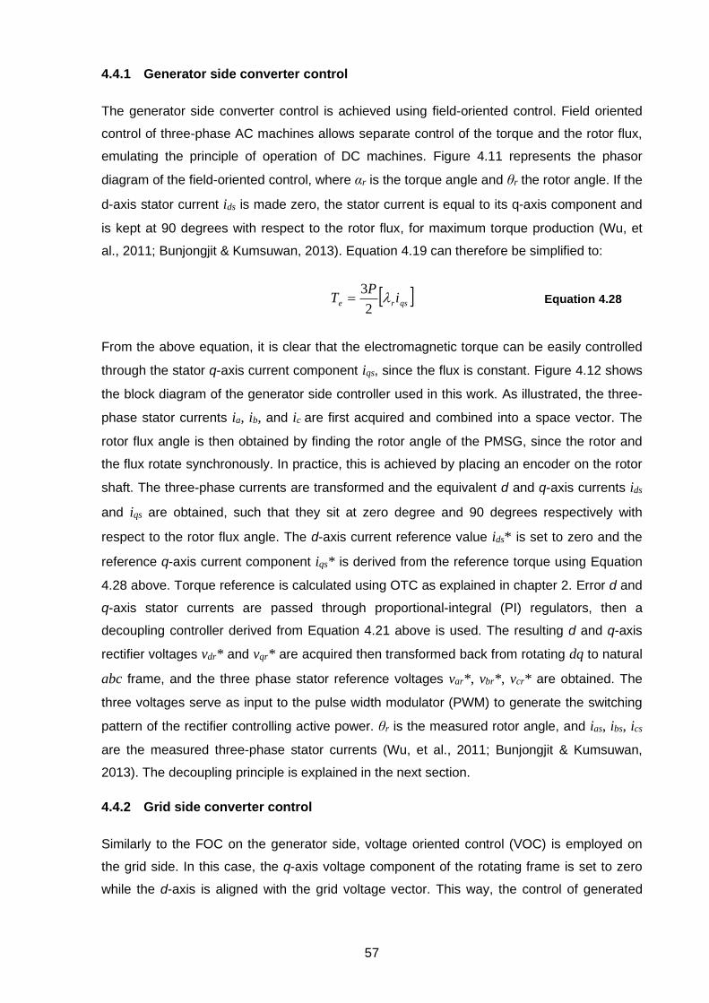
57
4.4.1 Generator side converter control
The generator side converter control is achieved using field-oriented control. Field oriented
control of three-phase AC machines allows separate control of the torque and the rotor flux,
emulating the principle of operation of DC machines. Figure 4.11 represents the phasor
diagram of the field-oriented control, where αr is the torque angle and θr the rotor angle. If the
d-axis stator current ids is made zero, the stator current is equal to its q-axis component and
is kept at 90 degrees with respect to the rotor flux, for maximum torque production (Wu, et
al., 2011; Bunjongjit & Kumsuwan, 2013). Equation 4.19 can therefore be simplified to:
qsre iP
T 2
3= Equation 4.28
From the above equation, it is clear that the electromagnetic torque can be easily controlled
through the stator q-axis current component iqs, since the flux is constant. Figure 4.12 shows
the block diagram of the generator side controller used in this work. As illustrated, the three-
phase stator currents ia, ib, and ic are first acquired and combined into a space vector. The
rotor flux angle is then obtained by finding the rotor angle of the PMSG, since the rotor and
the flux rotate synchronously. In practice, this is achieved by placing an encoder on the rotor
shaft. The three-phase currents are transformed and the equivalent d and q-axis currents ids
and iqs are obtained, such that they sit at zero degree and 90 degrees respectively with
respect to the rotor flux angle. The d-axis current reference value ids* is set to zero and the
reference q-axis current component iqs* is derived from the reference torque using Equation
4.28 above. Torque reference is calculated using OTC as explained in chapter 2. Error d and
q-axis stator currents are passed through proportional-integral (PI) regulators, then a
decoupling controller derived from Equation 4.21 above is used. The resulting d and q-axis
rectifier voltages vdr* and vqr* are acquired then transformed back from rotating dq to natural
abc frame, and the three phase stator reference voltages var*, vbr*, vcr* are obtained. The
three voltages serve as input to the pulse width modulator (PWM) to generate the switching
pattern of the rectifier controlling active power. θr is the measured rotor angle, and ias, ibs, ics
are the measured three-phase stator currents (Wu, et al., 2011; Bunjongjit & Kumsuwan,
2013). The decoupling principle is explained in the next section.
4.4.2 Grid side converter control
Similarly to the FOC on the generator side, voltage oriented control (VOC) is employed on
the grid side. In this case, the q-axis voltage component of the rotating frame is set to zero
while the d-axis is aligned with the grid voltage vector. This way, the control of generated

58
active power is ensured by the d-axis, while the reactive power control depends on and q-
axis current components respectively as expressed in Equation 4.29 (Wu, et al., 2011).
)(2
3
)(2
3
qgdgdgqgg
qgqgdgdgg
ivivQ
ivivP
−=
+=
Equation 4.29
EdcVdc
+
_
ibsvbg
Gen side rectifier
Ls
iasvag
icsvcg
var
vbr
vcr
PWM
dq/abc
PI PI
ωr (λ
r+L d
s)
ωr L
qs
var* vbr* vcr*
vdrvqr
idsiqs
ids* =0
iqs*
Vdc
idg iqg
θr
Rdc
+
_
Cross-coupling
PMSG
abc/dq
1
1.5Pλrωr
2 kopt
Te*ωr
θr ωr
Rs
Figure 4.12: Generator side converter control

59
EdcVdc
+
_
ibg vbg
Grid
Grid side inverter
Lg iag vag
icg vcg
vai
vbi
vci
PWM
dq/abc abc/dq
PLL
PI PIωgLg ωgLg
PI
./.
vai* vbi* vci*
vdi vqi
vdg vqg
idg iqgidg*
iqg*
Vdc Vdc*
Vdc
vdg vqg idg iqg
-1.5vdg
Qg*
θg
Rdc
+
_
Decoupled controller
Figure 4.13: Grid side converter control
Since vqg is set to zero, the grid active and reactive powers can be simplified as:
qgdgg
dgdgg
ivQ
ivP
2
3
2
3
−=
=
Equation 4.30

60
If the converter losses are neglected, it can be assumed that the active power is the same on
both DC and AC sides of the inverter. Therefore, Pg in Equation 4.29 above can be rewritten
as:
dcdcg ivP
2
3=
Equation 4.31
Equation 4.31 shows that the reference grid d-axis current can be used for the control of the
DC-link voltage vdc. On the other side, the q-axis current component can be derived from Qg
in Equation 4.32 as:
dg
g
qgv
Qi
3
2−= Equation 4.32
The block diagram of the grid side control is presented in Figure 4.13. As illustrated, the
control uses two main external feedback loops, one for the control of the DC link voltage and
the other for the control of reactive power. Two internal current control loops are also
available for the control of d and q current components generated from the DC link voltage
and the reactive power respectively (Wu, et al., 2011).
The three-phase grid voltages and currents, as well as the DC-link voltage measurements
are first acquired. In order to realise reference frame transformations from abc to dq and vice
versa, the grid voltage vector angle θg is needed. The phase locked loop (PLL) technique is
therefore applied to track the grid voltage vector and extract its angle (Wu, et al., 2011). The
dq equations of the grid voltages are expressed as:
qidgggqggqggqg
diqgggdggdggdg
viLidt
dLiRv
viLidt
dLiRv
+++=
+−+=
Equation 4.33
where vdi and vqi represent the d and q-axis inverter voltages respectively, ωg the grid
angular velocity, Rg and Lg the grid resistance and inductance respectively. The above
equation shows the cross-coupling nature of the system control, since both d and q terms are
present in each one of the expressions vgd and vgq. Consequently, a decoupling controller is
used to ease calculations and improve the dynamic response of the controller (Wu, et al.,
2011).
Rearranging the terms in Equation 4.33, Equation 4.34 is obtained as:

61
qgdgggqggqggqi
dgqgggdggdggdi
viLidt
dLiRv
viLidt
dLiRv
+−+−=
+++−=
)(
)(
Equation 4.34
Considering the PI nature of the controllers, Equation 4.34 can be rewritten as:
qgdgggqgqg
iiq
ipqqi
dgqgggdgdgiid
ipddi
viLiis
kkv
viLiis
kkv
+−−+−=
++−+−=
))((
))((
*
*
Equation 4.35
where idg* and iqg* are the d and q-axis reference currents, kipd and kiid are the d-axis
proportional and integral gains, kipq and kiiq are the q-axis proportional and integral gains
respectively. Rearranging Equation 4.34 andEquation 4.35, and substituting the first one into
the second, the following expressions are obtained (Wu, et al., 2011):
))((
))((
*
*
qgqg
iiq
ipqqggqgg
dgdgiid
ipddggdgg
iis
kki
dt
dLiR
iis
kki
dt
dLiR
−+=+
−+=+
Equation 4.36
From the above equation, it can be noted that the d-axis and q-axis components are clearly
separated from each other, showing the decoupled nature of the control system. In Figure
4.13, vai*, vbi*, vci* are the reference inverter three phase voltages, vag, vbg, and vcg are the
measured grid three-phase voltages, iag, ibg, and icg, the measured grid three-phase currents
respectively (Wu, et al., 2011).
Vdc
S1 S3 S5
S2 S4 S6
a
b
c
LOAD
+
_
g1 g3 g5
g2 g4 g6
ia
ib
ic
n
Figure 4.14: Two-level voltage source converter topology
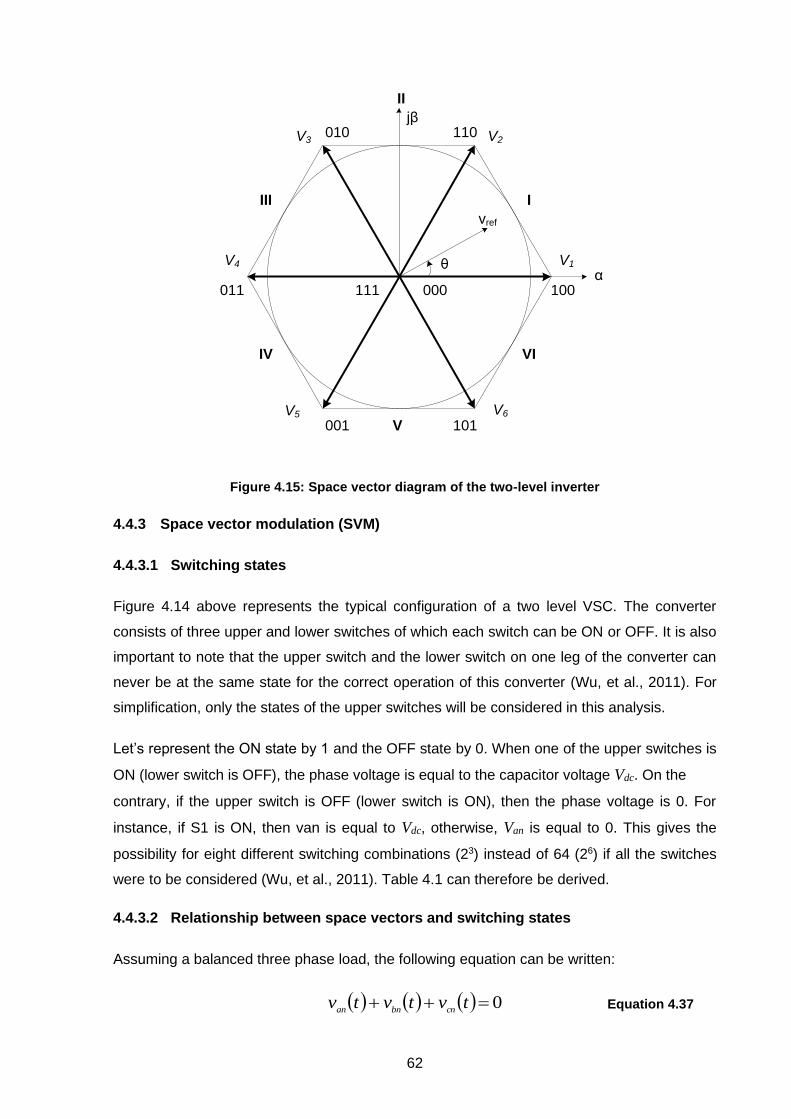
62
V1
V2V3
V4
V5 V6
I
II
III
IV
V
VI
110010
011 100
001 101
000111
vref
θ α
jβ
Figure 4.15: Space vector diagram of the two-level inverter
4.4.3 Space vector modulation (SVM)
4.4.3.1 Switching states
Figure 4.14 above represents the typical configuration of a two level VSC. The converter
consists of three upper and lower switches of which each switch can be ON or OFF. It is also
important to note that the upper switch and the lower switch on one leg of the converter can
never be at the same state for the correct operation of this converter (Wu, et al., 2011). For
simplification, only the states of the upper switches will be considered in this analysis.
Let’s represent the ON state by 1 and the OFF state by 0. When one of the upper switches is
ON (lower switch is OFF), the phase voltage is equal to the capacitor voltage Vdc. On the
contrary, if the upper switch is OFF (lower switch is ON), then the phase voltage is 0. For
instance, if S1 is ON, then van is equal to Vdc, otherwise, Van is equal to 0. This gives the
possibility for eight different switching combinations (23) instead of 64 (26) if all the switches
were to be considered (Wu, et al., 2011). Table 4.1 can therefore be derived.
4.4.3.2 Relationship between space vectors and switching states
Assuming a balanced three phase load, the following equation can be written:
( ) ( ) ( ) 0=++ tvtvtvcnbnan
Equation 4.37

63
Table 4.1: Switching states and output voltages of the inverter
Switching States Line to neutral voltages
a b c
Van
Vbn
Vcn S1 S3 S5
0 0 0 0 0 0
1 0 0 Vdc 0 0
1 1 0 Vdc Vdc 0
0 1 0 0 Vdc 0
0 1 1 0 Vdc Vdc
0 0 1 0 0 Vdc
1 0 1 Vdc 0 Vdc
1 1 1 Vdc Vdc Vdc
where van, vbn, and vcn represent the load three-phase voltages at an instant t. The three-
phase variables can be transformed into two-phase by applying the abc to αβ transformation
discussed in section 4.3.1, to obtain a space vector v(t) as expressed in Equation 4.39 (Wu,
et al., 2011):
( )
( )
( )
( )
( )
−
−−
=
tv
tv
tv
tv
tv
cn
bn
an
β
α.
2
3
2
30
2
1
2
11
3
2 Equation 4.38
Equation 4.39
Further developing expression Equation 4.38 and substitution into Equation 4.39 leads to:
( ) ( ) ( ) ( )tvjtvjtvtvcnbnan
+−
−−=
3
3
3
1
3
3
3
1
3
2 Equation 4.40
The above equation can also be written in exponential form as:
( ) ( ) ( ) ( )
++= 3
4
3
2
0
3
2 πj
cn
πj
bn
j
anetvetvetvtv
Equation 4.41
( ) ( ) ( )tjvtvtv +=

64
Table 4.2: Space vectors, switching states, and vectors definition
Vectors Switching states Vectors definition
V0 000 0
V1 100 dcV
3
2
V2 110 3
3
2 πj
dceV
V3 010 3
2
3
2 πj
dceV
V4 011 πj
dceV
3
2
V5 001 3
4
3
2 πj
dceV
V6 101 3
5
3
2 πj
dceV
V7 111 0
Considering the first active switching state in Table 4.1, van=Vdc, and vbn=vcn=0. Replacing
those values into Equation 4.41, the corresponding space vector V1 is obtained as:
dc
VV3
21=
Equation 4.42
Following the switching arrangement given in Table 4.1 above, the other space vector
expressions can be obtained as shown in Table 4.2 above. From this table, the space vector
diagram shown in Figure 4.16 can be generated. It is important to note the 60 degrees (π/3)
phase difference between the stationary active space vectors. Figure 4.16 also shows that a
reference vector vref can be produced from the two active space vectors and the zero space
vectors that constitute a section. For instance, vref in section I of the space vector diagram is
made of the active space vectors V1 and V2, and the zero space vector V0. The reference
vector vref is expressed as (Wu, et al., 2011):
j
refref evv .= Equation 4.43
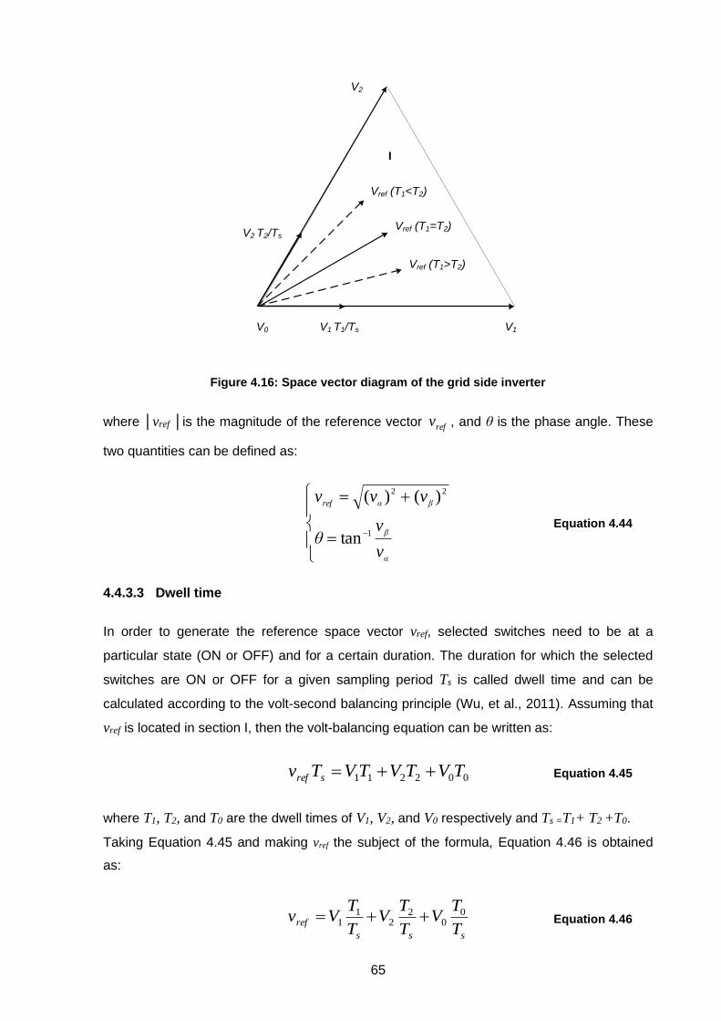
65
I
V1V0
V2
V1 T1/Ts
V2 T2/Ts
Vref (T1<T2)
Vref (T1=T2)
Vref (T1>T2)
Figure 4.16: Space vector diagram of the grid side inverter
where │vref │is the magnitude of the reference vector refv , and θ is the phase angle. These
two quantities can be defined as:
=
+=
−
α
β
βαref
v
vθ
vvv
1
22
tan
)()(
Equation 4.44
4.4.3.3 Dwell time
In order to generate the reference space vector vref, selected switches need to be at a
particular state (ON or OFF) and for a certain duration. The duration for which the selected
switches are ON or OFF for a given sampling period Ts is called dwell time and can be
calculated according to the volt-second balancing principle (Wu, et al., 2011). Assuming that
vref is located in section I, then the volt-balancing equation can be written as:
002211 TVTVTVTv sref ++= Equation 4.45
where T1, T2, and T0 are the dwell times of V1, V2, and V0 respectively and Ts =T1+ T2 +T0.
Taking Equation 4.45 and making vref the subject of the formula, Equation 4.46 is obtained
as:
sss
refT
TV
T
TV
T
TVv 0
02
21
1 ++= Equation 4.46

66
The above equation is illustrated in figure 4.16, where vref lies in sector I.
Substituting Equation 4.43 and the vectors definitions of vectors V1, V2, and V0 from Table 4.2
into Equation 4.45, Equation 4.47 is obtained as (Wu, et al., 2011):
3
213
2
3
2.
πj
dcdcs
θj
refeTVTVTev += Equation 4.47
The real and imaginary components of the above equation can be derived as:
=
+=
2
21
3
3sin
3
1
3
2cos
TVTv
TVTVTv
dcsref
dcdcsref
Equation 4.48
The dwell times can therefore be calculated using from Equation 4.49 below:
−−=
=
−=
210
2
1
sin3
3sin
3
TTTT
V
vTT
V
vTT
s
dc
refs
dc
refs
Equation 4.49
It is shown in Figure 4.16 that there is a relationship between vref and the magnitudes of the
dwell times. As such, the relationship between the location of vref and the dwell times can be
summarised as shown in
Table 4.4.
Table 4.3: Relationship between reference vector location and dwell times
vref location θ =0 0 < θ< π/6 θ = π/6 π/6 <θ < π/3 θ =π/3
Dwell times Ta >0; Tb =0 Ta >Tb Ta = Tb Ta <Tb Tb >0; Ta =0
Equation 4.49 above can be rewritten in terms of the modulation index ma as:
−−=
=
−=
210
2
1
sin
3sin
TTTT
mTT
mTT
s
as
as
Equation 4.50

67
where
dc
ref
aV
vm
=
3 Equation 4.51
111
2
1T
2
1T
2
2T
2
2T
4
0T
4
0T
2
0T
van
vbn
vcn
vab
0
0
0
0
Vdc
100 110 100110000 000
Vdc
Vdc
Vdc
Figure 4.17: Seven-segment switching sequence for reference vector located in sector I
Table 4.4: Seven segment switching sequence
Sector
Switching sequence
1 2 3 4 5 6 7
I
V0
000
V1
100
V2
110
V0
111
V2
110
V1
100
V0
000
II
V0
000
V3
010
V2
110
V0
111
V2
110
V3
010
V0
000
III
V0
000
V3
010
V4
011
V0
111
V4
011
V3
010
V0
000
IV
V0
000
V5
001
V4
011
V0
111
V4
011
V5
001
V0
000
V
V0
000
V5
001
V6
101
V0
111
V6
101
V5
001
V0
000
VI
V0
000
V1
100
V6
101
V0
111
V6
101
V1
100
V0
000

68
4.4.3.4 Switching sequence
With the space vectors selected and the dwell times calculated, the switching sequence of
the inverter can be obtained. Assuming that vref is located in sector I, the seven-segment
switching sequence in Figure 4.17 is derived.
Table 4.4 summarises the switching sequence for all the seven sectors (Wu, et al., 2011).
Summary of the chapter
This chapter presented the mathematical modelling of the PMSG based WECS used in this
work. Each section of the WECS was modelled separately from the mechanical turbine rotor
and drive train, to the electrical generator and power converters. On the mechanical side, the
turbine model equations were presented. The two-mass model implemented on the drive
train was also discussed. On the electrical side both steady-state and dynamic models of the
PMSG were discussed. Modelling equations and phasor diagram were derived and used for
FOC of the generator side rectifier. The grid side inverter was also modelled using VOC and
modelling equations were discussed. Finally, the space vector modulation used for the
control of converters was presented and explained.

69
CHAPTER FIVE
5 SIMULATION RESULTS AND DISCUSSIONS
Introduction
In this chapter, simulation results for the proposed fault ride-through methods employed are
presented and discussed. Different scenarios are implemented to gauge the capacity of the
system in achieving LVRT or not. A description of the complete power system is first given.
The system modelling presented in the previous chapter is then validated through
simulations under normal operating conditions (without grid disturbance), before simulations
during grid faults are carried through. Finally, the results are analysed and compared, and
small conclusions are drawn.
5.1 Power system configuration
The simulation model was developed using Simpowersystem, the power systems simulation
tool of Matlab/Simulink. The complete power system and wind turbine models are presented
in appendix B. Figure 5.1 is the single line diagram of the complete power system used for
the simulation studies The system consists of 6 x 1.5 MW wind turbines each connected to a
25 kV feeder through a 2 MVA transformer and 10 km transmission line. The 25 kV feeder
supplies power to the 120kV grid using a 20 km transmission line and a 47 MVA step-up
transformer. The grid is represented by a three-phase voltage source. The system
parameters are presented in appendix A.
9 MW wind
farm
10 km line20 km lineT1T2
Bus 1Bus 2Bus 3
PCC
Grid
690 V25 kV120 kV6 x 1.5 MW
PMSG WTs
25 kV/690 V
6 x 2 MVA
120 kV/25 kV
47 MVA
120 kV
2500 MVA
Figure 5.1: Single line diagram of the electric power system under study

70
5.2 Wind farm model aggregation
The wind farm model used in this work is an aggregated model consisting of a representation
of many individual wind turbines lumped into one unit, as opposed to a detailed model in
which every single turbine is represented and modelled separately. In fact, with the detailed
model, simulations become more complex due the increased overall system’s complexity
and simulation time, while the model aggregated technique is simpler and faster, still without
compromising the accuracy of the results (Qiao, et al., 2007; Sanchez, et al., 2012).
As explained in literature (Koc, 2010), only electrical components are affected during model
aggregation. Mechanical and aerodynamic parameters are not considered for aggregation.
As a result, generator parameters such as rotor inertia, friction coefficient, pole pairs, turbine
mechanical parameters and the pitch control system remain unchanged.
To achieve proper model aggregation, generator and converter power ratings are multiplied
by the number of turbines in the wind farm, while resistive parameters are divided by this
number to supply new rated current. It is also assumed, for more simplicity that the wind the
direction of the wind and the rotational speed are the same for all the individual wind turbines
(Koc, 2010).
5.3 Simulation results under normal operating conditions
At first, the wind turbine system is tested under normal operating conditions to validate the
effectiveness of the generator and grid side converter controllers in achieving MPPT and DC-
link and reactive power control respectively. As such, the varying step wind speed profile
shown in Figure 5.2 is used as input to the turbine model. The wind speed increases from 9
to 11 m/s with a 1 m/s increment rate then decreases back from 11 m/s to 9 m/s at the same
rate, every 2 seconds. The pitch angle is maintained at maximum value (zero degree).
The results displayed show that MPPT is successfully achieved by the generator side
converter. As shown in Figure 5.3, the generator mechanical speed varies according to the
change in wind speed. At 11 m/s, the generator speed is equal to 1 p.u, then 0.91 p.u and
0.82 p,u respectively at 10 m/s and 9 m/s. These values correspond to the maximum per unit
generator speed values for each wind speed. The mechanical torque is also displayed in
Figure 5.4. Since torque control is used for MPPT, the torque variation also follows the wind
speed input. The negative values indicate that the PMSM operates in the generator mode. In
figures 5.5 and 5.6, the responses of the power coefficient and tip speed ratio are shown. As
expected, the power coefficient remains constant at its rated value of 0.48 despite changes
in wind speed, ensuring maximum power production from the turbine at lower and rated wind
speeds. The tip speed ratio also remains constant at 8.1.
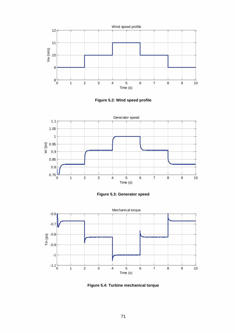
71
Figure 5.2: Wind speed profile
Figure 5.3: Generator speed
Figure 5.4: Turbine mechanical torque
0 1 2 3 4 5 6 7 8 9 108
9
10
11
12
Time (s)
Vw
(m
/s)
Wind speed profile
0 1 2 3 4 5 6 7 8 9 100.75
0.8
0.85
0.9
0.95
1
1.05
1.1Generator speed
Time (s)
wr
(pu)
0 1 2 3 4 5 6 7 8 9 108
9
10
11
12
Time (s)
Vw
(m
/s)
Wind speed profile
0 1 2 3 4 5 6 7 8 9 100.75
0.8
0.85
0.9
0.95
1
1.05
1.1Generator speed
Time (s)
wr
(pu)
0 1 2 3 4 5 6 7 8 9 10-1.1
-1
-0.9
-0.8
-0.7
-0.6
Time (s)
Tm
(p
u)
Mechanical torque
0 0.1 0.2 0.3 0.4 0.5 0.6 0.7 0.8 0.9 10
0.2
0.4
0.6
0.8
1

72
Figure 5.5: Wind turbine's power coefficient
Figure 5.6: Wind turbie's tip speed ratio
Figure 5.7: Three phase stator voltages
0 1 2 3 4 5 6 7 8 9 100.45
0.46
0.47
0.48
0.49
0.5
Time (s)
Cp
Power coefficient
0 1 2 3 4 5 6 7 8 9 105
6
7
8
9
10Tip speed ratio
Time (s)
Lam
bda
0 1 2 3 4 5 6 7 8 9 100.45
0.46
0.47
0.48
0.49
0.5
Time (s)
Cp
Power coefficient
0 1 2 3 4 5 6 7 8 9 105
6
7
8
9
10Tip speed ratio
Time (s)
Lam
bda
0 1 2 3 4 5 6 7 8 9 10
-1
-0.5
0
0.5
1
Time (s)
Vab
c (
pu
)
Three-phase stator voltages

73
Figure 5.8: Three phase stator currents
As far as the electrical parameters are concerned, the three-phase stator voltages and
currents are displayed on Figure 5.7 and 5.8 respectively. These results show that the
voltages are proportional to the generator speed, while the currents are proportional to the
mechanical torque, both in magnitude. The stator power is also shown in Figure 5.9. The d-
axis and q-axis stator currents are shown with their references in Figure 5.10. The d-axis
current is constant at 0 p.u, to achieve zero d-axis current control and magnitude of the q-
axis current is equal to the stator current as expected.
Figure 5.9: Stator active power
0 1 2 3 4 5 6 7 8 9 10
-1
-0.5
0
0.5
1
Time (s)
Iabc (
pu
)
Three-phase stator currents
4.7 4.71 4.72 4.73 4.74 4.75 4.76 4.77 4.78 4.79 4.8
-1
-0.5
0
0.5
1
Time (s)
Iabc (
pu
)
Three-phase grid currents
0 1 2 3 4 5 6 7 8 9 100
0.2
0.4
0.6
0.8
1
Stator power
Time (s)
Ps
(pu)
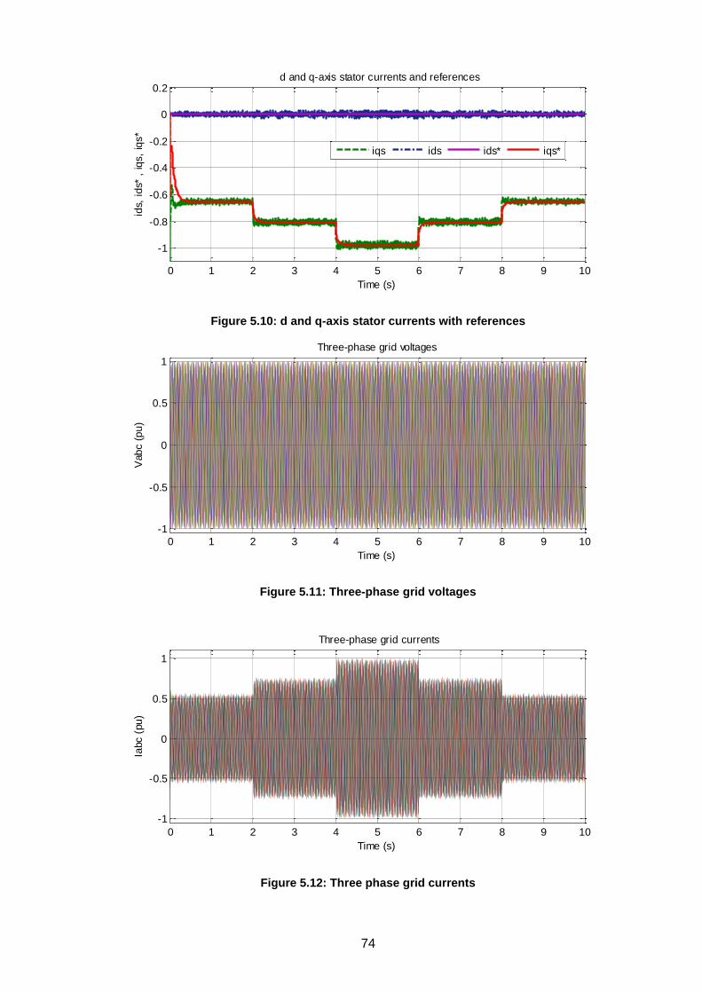
74
Figure 5.10: d and q-axis stator currents with references
Figure 5.11: Three-phase grid voltages
Figure 5.12: Three phase grid currents
0 1 2 3 4 5 6 7 8 9 10
-1
-0.8
-0.6
-0.4
-0.2
0
0.2
Time (s)
ids,
id
s* ,
iq
s,
iqs*
d and q-axis stator currents and references
iqs ids ids* iqs*
0 0.1 0.2 0.3 0.4 0.5 0.6 0.7 0.8 0.9 10
0.2
0.4
0.6
0.8
1
0 1 2 3 4 5 6 7 8 9 10
-1
-0.5
0
0.5
1
Time (s)
Vab
c (
pu
)
Three-phase grid voltages
0 0.1 0.2 0.3 0.4 0.5 0.6 0.7 0.8 0.9 10
0.2
0.4
0.6
0.8
1
0 1 2 3 4 5 6 7 8 9 10
-1
-0.5
0
0.5
1
Time (s)
Iabc (
pu
)
Three-phase grid currents
0 0.1 0.2 0.3 0.4 0.5 0.6 0.7 0.8 0.9 10
0.2
0.4
0.6
0.8
1

75
Figure 5.13: DC-link voltage
Figure 5.14: Current through DC-link
Figure 5.15: DC-link power
0 1 2 3 4 5 6 7 8 9 10
0.6
0.8
1
1.2
1.4
Time (s)
Vdc (
pu
)
DC-link voltage
0 1 2 3 4 5 6 7 8 9 100
0.2
0.4
0.6
0.8
1
Grid active power
Time (s)
Pgri
d (
pu
)
0 1 2 3 4 5 6 7 8 9 10
-1
-0.5
0
0.5
1
Time (s)
Pdc (
pu
)
DC-link power
0 1 2 3 4 5 6 7 8 9 10-1
-0.5
0
0.5
1x 10
-3DC-link current
Time (s)
Idc
(pu)
0 1 2 3 4 5 6 7 8 9 10
-1
-0.5
0
0.5
1
Time (s)
Pdc (
pu
)
DC-link power
0 1 2 3 4 5 6 7 8 9 10-1
-0.5
0
0.5
1x 10
-3DC-link current
Time (s)
Idc
(pu)
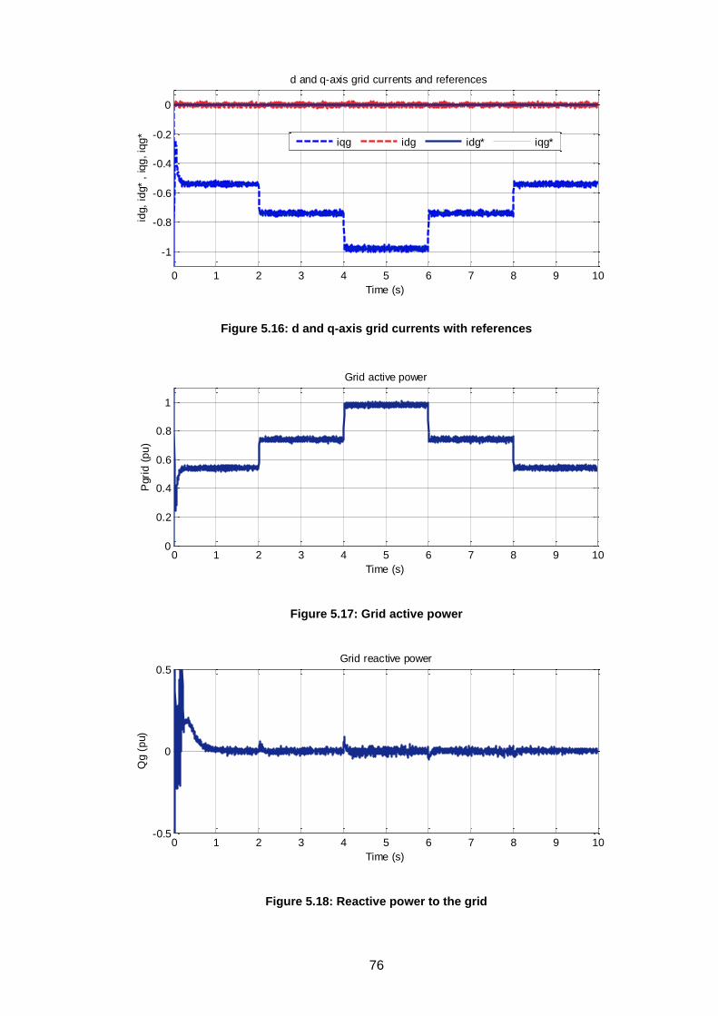
76
Figure 5.16: d and q-axis grid currents with references
Figure 5.17: Grid active power
Figure 5.18: Reactive power to the grid
0 1 2 3 4 5 6 7 8 9 10
-1
-0.8
-0.6
-0.4
-0.2
0
Time (s)
idg,
idg*
, iq
g,
iqg
*
d and q-axis grid currents and references
iqg idg idg* iqg*
0 0.1 0.2 0.3 0.4 0.5 0.6 0.7 0.8 0.9 10
0.2
0.4
0.6
0.8
1
0 1 2 3 4 5 6 7 8 9 10
0.6
0.8
1
1.2
1.4
Time (s)
Vdc (
pu
)
DC-link voltage
0 1 2 3 4 5 6 7 8 9 100
0.2
0.4
0.6
0.8
1
Grid active power
Time (s)
Pgri
d (
pu
)
0 1 2 3 4 5 6 7 8 9 1058
58.5
59
59.5
60
60.5
61
Time (s)
f (H
z)
Grid frequency
0 1 2 3 4 5 6 7 8 9 10-0.5
0
0.5Grid reactive power
Time (s)
Qg (
pu)
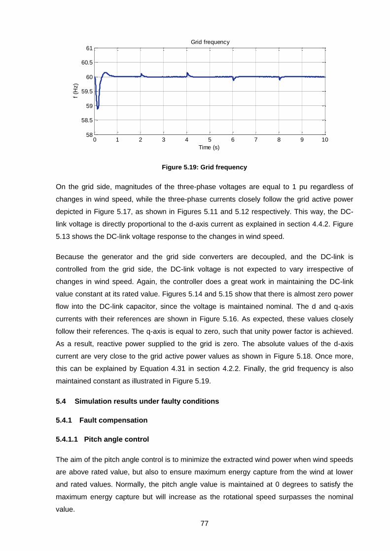
77
Figure 5.19: Grid frequency
On the grid side, magnitudes of the three-phase voltages are equal to 1 pu regardless of
changes in wind speed, while the three-phase currents closely follow the grid active power
depicted in Figure 5.17, as shown in Figures 5.11 and 5.12 respectively. This way, the DC-
link voltage is directly proportional to the d-axis current as explained in section 4.4.2. Figure
5.13 shows the DC-link voltage response to the changes in wind speed.
Because the generator and the grid side converters are decoupled, and the DC-link is
controlled from the grid side, the DC-link voltage is not expected to vary irrespective of
changes in wind speed. Again, the controller does a great work in maintaining the DC-link
value constant at its rated value. Figures 5.14 and 5.15 show that there is almost zero power
flow into the DC-link capacitor, since the voltage is maintained nominal. The d and q-axis
currents with their references are shown in Figure 5.16. As expected, these values closely
follow their references. The q-axis is equal to zero, such that unity power factor is achieved.
As a result, reactive power supplied to the grid is zero. The absolute values of the d-axis
current are very close to the grid active power values as shown in Figure 5.18. Once more,
this can be explained by Equation 4.31 in section 4.2.2. Finally, the grid frequency is also
maintained constant as illustrated in Figure 5.19.
5.4 Simulation results under faulty conditions
5.4.1 Fault compensation
5.4.1.1 Pitch angle control
The aim of the pitch angle control is to minimize the extracted wind power when wind speeds
are above rated value, but also to ensure maximum energy capture from the wind at lower
and rated values. Normally, the pitch angle value is maintained at 0 degrees to satisfy the
maximum energy capture but will increase as the rotational speed surpasses the nominal
value.
0 1 2 3 4 5 6 7 8 9 1058
58.5
59
59.5
60
60.5
61
Time (s)
f (H
z)
Grid frequency
0 1 2 3 4 5 6 7 8 9 10-0.5
0
0.5Grid reactive power
Time (s)
Qg (
pu)

78
Pitch angle limiterPitch rate
ββrefωref
ωr
PITime
constant
Figure 5.20: Block diagram of the pitch angle controller
Figure 5.20 represents a block diagram of the operation of the pitch angle control system.
The reference rotor speed ωmref is compared to the actual measured speed ωm, and the error
signal is sent to a PI controller to produce the reference pitch angle βref. This reference is in
turn compared to the actual pitch angle value, and the error signal is used to correct the pitch
angle to the desired value.
However, practically, the blade pitch angle rotation is limited in range and speed. The design
therefore takes into consideration the actuators servo mechanism time constant, the pitch
angle limits (0 to 30 deg) and rate of change (±10 deg/s).
5.4.1.2 DC-link protection
During a grid fault, since the converters are decoupled, the DC-link capacitor will overcharge
due to the continuous power supply from the generator. The braking resistor is used to
dissipate this excess energy and thus keeping the DC-link and the converters safe. Normally,
the DC-link voltage must be kept within the limits of the converters and the capacitor, which
is around ±25% of its rated value, to avoid damage of the converters.
Assuming the converter operates at 100% of generator rated power, the braking resistor
should be designed to dissipate rated power of the turbine and in this case its value would be
equal to 0.96Ω. For the braking resistor’s controller, in order to obtain worst case scenario
results, the maximum allowable DC-link voltage is fixed to 1500V (1.25 pu) which
corresponds to 25% of the rated DC-link voltage.
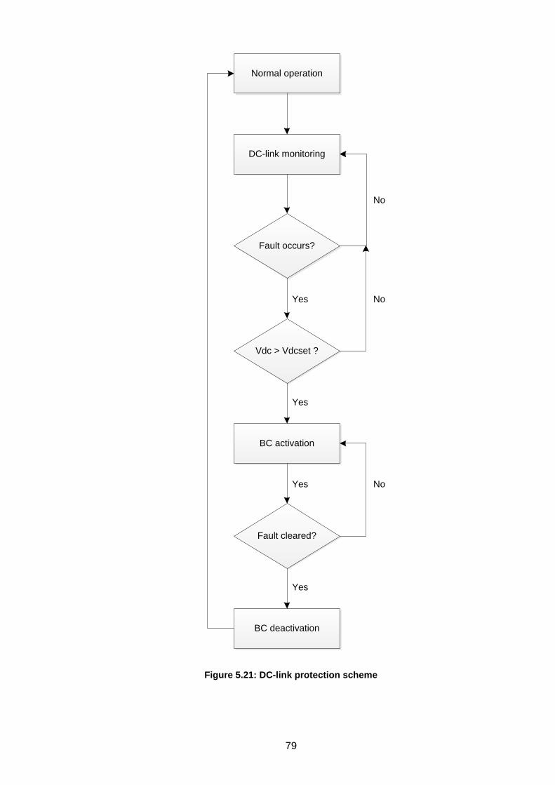
79
Normal operation
Fault occurs?
DC-link monitoring
Vdc > Vdcset ?
BC activation
Fault cleared?
BC deactivation
Yes
Yes
Yes
Yes
No
No
No
Figure 5.21: DC-link protection scheme

80
Normal operation
Fault occurs?
PCC voltage monitoring
Vpcc < Vpccset ?
Reactive current
injection
Fault cleared?
Unity power factor
operation
Yes
Yes
Yes
Yes
No
No
No
Figure 5.22: Grid reactive power support scheme

81
To control the switching of the resistor, the DC-link voltage value is measured and compared
to a predefined value set not exceeding 1.2 pu. As long as the Vdc remains within the normal
range, the controller sends a “0” signal and the braking resistor stays inactivated. Otherwise,
a trip signal “1” is immediately sent to the resistor’s switch and the excess stator current
starts flowing through the braking resistor instead of overcharging the capacitor. This control
is illustrated in Figure 5.21 above.
5.4.1.3 Reactive power compensation
The reactive current support requirement during grid fault is presented in Figure 3.9 of
section 3.1.5. As illustrated, when the grid voltage is comprised between 0.9 p.u and 1.1 p.u,
no reactive power compensation is necessary. That portion corresponds to area A. For grid
voltages below 0.9 p.u down to 0.5 p.u, reactive current injection is required to increase as a
function of the dip level, constituting area B. Finally in area C (for grid voltages below 0.5 p.u)
100 percent reactive current contribution expected. Figure 5.22 above shows the flow
diagram of how LVRT compensation is achieved.
5.4.2 Case studies for simulations under grid faults
To assess the effectivenes and robustness of the wind farm system to comply with the LVRT
requirements presented earlier in section 3.1, different case scenarios are considered. These
different scenarios are classified according to the location, the type, the dip level and
duration, and eventually the wind speed conditions. The results are also compared
depending on whether reactive current is injected according to Figure 3.9 to support grid
recovery or not, for the different LVRT methods tested.
Figure 5.23: Voltage profile during fault at bus 3 for case 1
1 1.5 2 2.5 3
-1
-0.5
0
0.5
1
Time (s)
Vbu
s3 (
pu
)
Three-phase voltages at bus 3
0 0.1 0.2 0.3 0.4 0.5 0.6 0.7 0.8 0.9 10
0.2
0.4
0.6
0.8
1
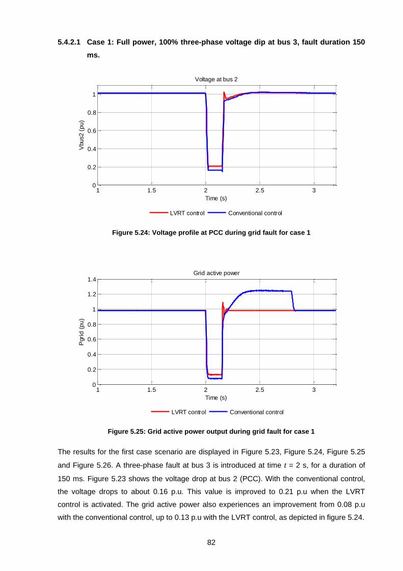
82
5.4.2.1 Case 1: Full power, 100% three-phase voltage dip at bus 3, fault duration 150
ms.
Figure 5.24: Voltage profile at PCC during grid fault for case 1
Figure 5.25: Grid active power output during grid fault for case 1
The results for the first case scenario are displayed in Figure 5.23, Figure 5.24, Figure 5.25
and Figure 5.26. A three-phase fault at bus 3 is introduced at time t = 2 s, for a duration of
150 ms. Figure 5.23 shows the voltage drop at bus 2 (PCC). With the conventional control,
the voltage drops to about 0.16 p.u. This value is improved to 0.21 p.u when the LVRT
control is activated. The grid active power also experiences an improvement from 0.08 p.u
with the conventional control, up to 0.13 p.u with the LVRT control, as depicted in figure 5.24.
1 1.5 2 2.5 30
0.2
0.4
0.6
0.8
1
Time (s)
Vbu
s2 (
pu
)Voltage at bus 2
1 1.5 2 2.5 30
0.5
1
1.5Grid active power
Time (s)
Pgri
d (
pu
)
LVRT control Conventional control1 1.5 2 2.5 3
0
0.5
1
Time (s)
Vbu
s2 (
pu
)
Voltage at bus 2
1 1.5 2 2.5 30
0.2
0.4
0.6
0.8
1
1.2
1.4Grid active power
Time (s)
Pgri
d (
pu
)
LVRT control Conventional control

83
Figure 5.26: DC-link voltage during grid fault for case 1
Figure 5.27: Grid reactive power output during grid fault for case 1
Moreover, after fault clearance and under conventional control, the active power to the grid
reaches about 1.25 p.u and is maintained at that value until time t = 2.8 s, before dropping
back to nominal value. This situation can be explained from the DC-link behaviour as
illustrated in Figure 5.26. During the fault duration, the generator’s speed is not affected by
the low voltage condition on the grid side due to the decoupled nature of the controllers,
causing the DC-link to rise uncontrollably when no additional action is applied as explained in
section 3.2. As a result, the DC-link voltage rises up to a value of about 3.81 p.u. After fault
clearance, the DC-link voltage decreases progressively until it reaches back its nominal
value of 1 p.u at time t = 2.8 s. During this recovery time, the surplus power stored in the DC-
1 1.5 2 2.5 30
0.2
0.4
0.6
0.8
1
1.2
1.4Grid active power
Time (s)
Pgri
d (
pu
)
LVRT control Conventional control
1 1.5 2 2.5 3
1
1.5
2
2.5
3
3.5
Time (s)
Vdc (
pu
)
DC-link voltage
1 1.5 2 2.5 30
0.2
0.4
0.6
0.8
1
1.2
1.4Grid active power
Time (s)
Pgri
d (
pu
)
LVRT control Conventional control
1 1.5 2 2.5 3
-0.4
-0.2
0
0.2
0.4
0.6Grid reactive power
Time (s)
Qgri
d (
pu
)
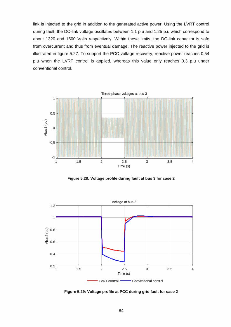
84
link is injected to the grid in addition to the generated active power. Using the LVRT control
during fault, the DC-link voltage oscillates between 1.1 p.u and 1.25 p.u which correspond to
about 1320 and 1500 Volts respectively. Within these limits, the DC-link capacitor is safe
from overcurrent and thus from eventual damage. The reactive power injected to the grid is
illustrated in figure 5.27. To support the PCC voltage recovery, reactive power reaches 0.54
p.u when the LVRT control is applied, whereas this value only reaches 0.3 p.u under
conventional control.
Figure 5.28: Voltage profile during fault at bus 3 for case 2
Figure 5.29: Voltage profile at PCC during grid fault for case 2
1 1.5 2 2.5 3 3.5 4
-1
-0.5
0
0.5
1
Time (s)
Vbu
s3 (
pu
)
Three-phase voltages at bus 3
0 0.1 0.2 0.3 0.4 0.5 0.6 0.7 0.8 0.9 10
0.2
0.4
0.6
0.8
1
1 1.5 2 2.5 30
0.2
0.4
0.6
0.8
1
1.2
1.4Grid active power
Time (s)
Pgri
d (
pu
)
LVRT control Conventional control
1 1.5 2 2.5 3 3.5 40.2
0.4
0.6
0.8
1
1.2
Time (s)
Vbu
s2 (
pu
)
Voltage at bus 2

85
Figure 5.30: Grid active power output during grid fault for case 2
5.4.2.2 Case 2: Full power, 65 % three-phase voltage dip at bus 3, fault duration 500
ms.
In this case, a 500 ms three-phase fault, with an amplitude of 0.65 p.u is applied at bus 3 as
illustrated in figure 5.28, at rated wind speed. Figure 5.29 depicts the behaviour of the
voltage at bus 2 during grid fault under the conditions specified in case 2. With the
conventional control, the PCC voltage drops directly to 0.4 p.u then continues to further
decrease to 0.28 p.u until the fault is cleared. However, with the LVRT control, the PCC
voltage curve shows a considerable improvement with values between 0.45 p.u and 0.5 p.u
during the voltage drop. In Figure 5.30, the active power responses of both controls are
presented. The active power to the grid shows a similar response to the PCC voltage. Under
conventional control, this power suddenly drops to 0.5 p.u directly at fault occurrence,
followed by a continuous decrease up to 0.28 p.u at fault clearance. Again, there is a
limitation to about 1.25 p.u during the whole DC-link recovery time. However, the active
power drop during the fault is improved to about 0.68 p.u when the LVRT control is activated,
and recovery to rated value is almost instantaneous after the fault is removed.In Figure 5.31,
the DC-link voltage is presented. Without LVRT compensation, the DC-link voltage rises
even more than in case 1 (5.4 p.u against 3.81p.u), while the capacitor’s discharge time at
fault clearance is also increased from 650 ms in case 1 to 1200 ms in the current case, which
is understandable because of the increased fault duration. On the other hand, DC-link
protection is satisfactorily achieved under LVRT control and the values are maintained within
acceptable limits as in the previous case. The reactive power shown in Figure 5.32 peaks to
0.2 p.u immediately when the fault occurs then ramps down to 0 pu with the conventional
controller, due to the lower grid voltage dip. With the LVRT control, this value peaks at 0.76
1 1.5 2 2.5 30
0.2
0.4
0.6
0.8
1
1.2
1.4Grid active power
Time (s)
Pgri
d (
pu
)
LVRT control Conventional control
1 1.5 2 2.5 3 3.5 40.2
0.4
0.6
0.8
1
1.2
1.4
Grid active power
Time (s)
Pgri
d (
pu
)

86
Figure 5.31: DC-link voltage during grid fault for case 2
Figure 5.32: Grid reactive power output during grid fault for case 2
pu showing that more reactive power is injected for grid support in this case compared to the
previous one, as expected from the reactive power requirement.
5.4.2.3 Case 3: Full power, 25 % three-phase voltage dip at bus 3, fault duration 1500
ms.
A 25 % three-phase grid voltage drop lasting 1.5 s is applied at bus 3 as shown in Figure
5.33. This time the fault level is reduced, however the duration is much prolonged. The PCC
voltage depicted in Figure 5.34 dips down to 0.75 p.u under conventional control, and 0.81
p.u when the LVRT control is applied, showing a voltage contribution of about 0.06 p.u.
1 1.5 2 2.5 30
0.2
0.4
0.6
0.8
1
1.2
1.4Grid active power
Time (s)
Pgri
d (
pu
)
LVRT control Conventional control
1 1.5 2 2.5 3 3.5 4
1
2
3
4
5
6DC-link voltage
Time (s)
Vdc (
pu
)
1 1.5 2 2.5 30
0.2
0.4
0.6
0.8
1
1.2
1.4Grid active power
Time (s)
Pgri
d (
pu
)
LVRT control Conventional control
1 1.5 2 2.5 3 3.5 4
-0.8
-0.6
-0.4
-0.2
0
0.2
0.4
0.6
0.8
Time (s)
Qgri
d (
pu
)
Grid reactive power

87
Figure 5.33: Voltage profile during fault at bus 3 for case 3
Figure 5.34: Voltage profile at PCC during grid fault for case 3
As shown in Figure 5.35, the grid active power only drops to 0.92 p.u during fault, but still
overshoots at fault clearance to 1.25 p.u as in the previous cases, although in this case the
power remains to that value for about 350 ms only. With the LVRT control, the active power
does not deviate from the nominal value during fault, and the overshoot is also eliminated at
fault clearance. The DC-link voltage rises up to 3 p.u during the fault, then takes about 350
ms dropping back to nominal value as shown in Figure 3.36. This recovery time is
considerably short compared to the previous two cases certainly because of the much lower
voltage dip and also the longer fault duration in this case. However under LVRT control, the
DC-link voltage is maintained constant at 1 p.u during the grid voltage dip. As a result, the
1 1.5 2 2.5 3 3.5 4 4.5 5
-1
-0.5
0
0.5
1
Time (s)
Vbu
s3 (
pu
)
Three-phase voltages at bus 3
0 0.1 0.2 0.3 0.4 0.5 0.6 0.7 0.8 0.9 10
0.2
0.4
0.6
0.8
1
1 1.5 2 2.5 30
0.2
0.4
0.6
0.8
1
1.2
1.4Grid active power
Time (s)
Pgri
d (
pu
)
LVRT control Conventional control
1 1.5 2 2.5 3 3.5 4 4.5 50.7
0.75
0.8
0.85
0.9
0.95
1
1.05
1.1
Time (s)
Vbu
s2 (
pu
)
Voltage at bus 2
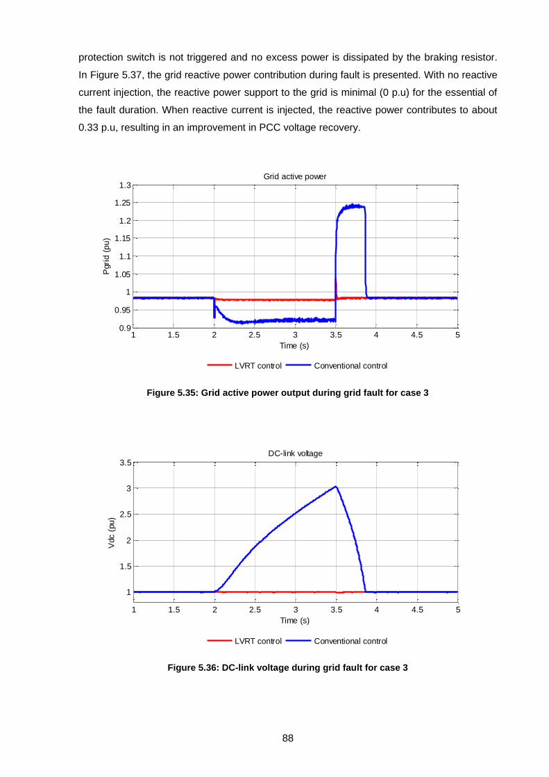
88
protection switch is not triggered and no excess power is dissipated by the braking resistor.
In Figure 5.37, the grid reactive power contribution during fault is presented. With no reactive
current injection, the reactive power support to the grid is minimal (0 p.u) for the essential of
the fault duration. When reactive current is injected, the reactive power contributes to about
0.33 p.u, resulting in an improvement in PCC voltage recovery.
Figure 5.35: Grid active power output during grid fault for case 3
Figure 5.36: DC-link voltage during grid fault for case 3
1 1.5 2 2.5 30
0.2
0.4
0.6
0.8
1
1.2
1.4Grid active power
Time (s)
Pgri
d (
pu
)
LVRT control Conventional control
1 1.5 2 2.5 3 3.5 4 4.5 50.9
0.95
1
1.05
1.1
1.15
1.2
1.25
1.3Grid active power
Time (s)
Pgri
d (
pu
)
1 1.5 2 2.5 30
0.2
0.4
0.6
0.8
1
1.2
1.4Grid active power
Time (s)
Pgri
d (
pu
)
LVRT control Conventional control
1 1.5 2 2.5 3 3.5 4 4.5 5
1
1.5
2
2.5
3
3.5DC-link voltage
Time (s)
Vdc (
pu
)

89
Figure 5.37: Grid reactive power output during grid fault for case 3
Figure 5.38: Voltage profile during fault at bus 3 for case 4
5.4.2.4 Case 4: Full power, 100% three-phase voltage dip at bus 3, fault duration 300
ms
For the fourth case scenario, the fault duration is extended to 300 ms for a voltage drop
down to 0 p.u, to evaluate the response of the system during a more severe fault as
illustrated in Figure 5.38. In Figure 5.39, when no reactive current is injected, the PCC
voltage drops to 0.16 p.u. At fault clearance, the PCC voltage experiences a quick
undershoot to about 0.05 p.u for less than 1 ms, before returning to normal operating region.
Under these conditions, the PCC voltage would fall outside the limits of the LVRT curve
presented in Figure 3.8 of section 3.1.5. With LVRT control, the PCC voltage improves to
1 1.5 2 2.5 30
0.2
0.4
0.6
0.8
1
1.2
1.4Grid active power
Time (s)
Pgri
d (
pu
)
LVRT control Conventional control
1 1.5 2 2.5 3 3.5 4 4.5 5-0.2
-0.1
0
0.1
0.2
0.3
0.4
0.5
0.6
Time (s)
Qgri
d (
pu
)
Grid reactive power
1 1.5 2 2.5 3 3.5 4 4.5 5
-1
-0.5
0
0.5
1
Time (s)
Vbu
s3 (
pu
)
Three-phase voltages at bus 3
0 0.1 0.2 0.3 0.4 0.5 0.6 0.7 0.8 0.9 10
0.2
0.4
0.6
0.8
1

90
0.21 p.u as in case 1. The undershoot is cleared, and the voltage profile falls back into the
LVRT curve limits. The grid active power in case 4 is shown in Figure 5.40. As in case 1, the
active power to the grid drops to 0.08 p.u under normal control. However at fault clearance,
its value quickly drops to 0 p.u, then ramps up to 1.25 p.u where it remains for 2 s before
reaching back nominal power. When LVRT control is employed, the drop is improved to 0.13
p.u and recovery after fault clearance is fast but not immediate, since there is a short
transient before ramping back to the normal operating state.
Figure 5.39: Voltage profile at PCC during grid fault for case 4
Figure 5.40: Grid active power output during grid fault for case 4
1 1.5 2 2.5 30
0.2
0.4
0.6
0.8
1
1.2
1.4Grid active power
Time (s)
Pgri
d (
pu
)
LVRT control Conventional control
1 1.5 2 2.5 3 3.5 4 4.5 50
0.2
0.4
0.6
0.8
1
Time (s)
Vbu
s2 (
pu
)
Voltage at bus 2
1 1.5 2 2.5 30
0.2
0.4
0.6
0.8
1
1.2
1.4Grid active power
Time (s)
Pgri
d (
pu
)
LVRT control Conventional control
1 1.5 2 2.5 3 3.5 4 4.5 5
0
0.2
0.4
0.6
0.8
1
1.2
Grid active power
Time (s)
Pgri
d (
pu
)
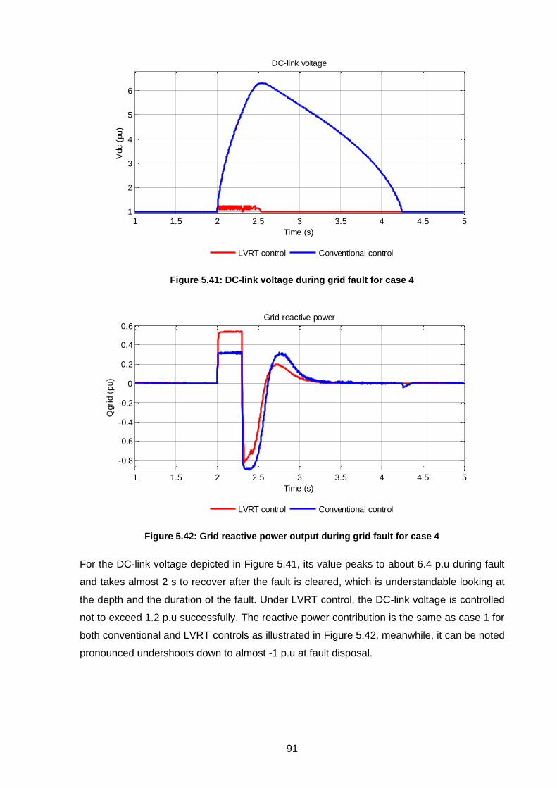
91
Figure 5.41: DC-link voltage during grid fault for case 4
Figure 5.42: Grid reactive power output during grid fault for case 4
For the DC-link voltage depicted in Figure 5.41, its value peaks to about 6.4 p.u during fault
and takes almost 2 s to recover after the fault is cleared, which is understandable looking at
the depth and the duration of the fault. Under LVRT control, the DC-link voltage is controlled
not to exceed 1.2 p.u successfully. The reactive power contribution is the same as case 1 for
both conventional and LVRT controls as illustrated in Figure 5.42, meanwhile, it can be noted
pronounced undershoots down to almost -1 p.u at fault disposal.
1 1.5 2 2.5 30
0.2
0.4
0.6
0.8
1
1.2
1.4Grid active power
Time (s)
Pgri
d (
pu
)
LVRT control Conventional control
1 1.5 2 2.5 3 3.5 4 4.5 51
2
3
4
5
6
DC-link voltage
Time (s)
Vdc (
pu
)
1 1.5 2 2.5 30
0.2
0.4
0.6
0.8
1
1.2
1.4Grid active power
Time (s)
Pgri
d (
pu
)
LVRT control Conventional control
1 1.5 2 2.5 3 3.5 4 4.5 5
-0.8
-0.6
-0.4
-0.2
0
0.2
0.4
0.6
Time (s)
Qgri
d (
pu
)
Grid reactive power

92
Figure 5.43: Voltage profile during fault at bus 3 for case 5
Figure 5.44: Voltage profile at PCC during grid fault for case 5
5.4.2.5 Case 5: Full power, 100% single line to groung voltage dip at bus 3, fault
duration 150 ms
In the fifth case scenario, a single-phase to ground fault is applied at bus 3 for 150 ms. The
single line fault is normally a less severe type because the other two phases can still
compensate for the one phase loss and operate safely without causing major disturbances.
Figure 5.43 shows how phase A drops down to about 0.1 p.u, while phases B and C remain
close to 1 p.u during the fault time interval from 2s to 2.15s.
0 0.1 0.2 0.3 0.4 0.5 0.6 0.7 0.8 0.9 10
0.2
0.4
0.6
0.8
1
1.9 1.95 2 2.05 2.1 2.15 2.2 2.25
-1
-0.5
0
0.5
1
Time (s)
Vbu
s3 (
pu
)
Three-phase voltages at bus 3
Va
Vb
Vc
1 1.5 2 2.5 30.6
0.65
0.7
0.75
0.8
0.85
0.9
0.95
1
1.05
Time (s)
Vbu
s2 (
pu
)
Voltage at bus 2
1 1.5 2 2.5 30.6
0.8
1
1.2
Grid active power
Time (s)
Pgri
d (
pu
)
LVRT control Conventional control
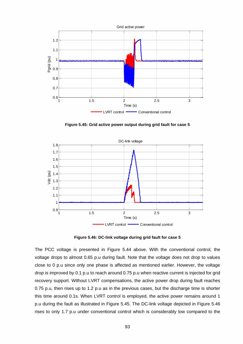
93
Figure 5.45: Grid active power output during grid fault for case 5
Figure 5.46: DC-link voltage during grid fault for case 5
The PCC voltage is presented in Figure 5.44 above. With the conventional control, the
voltage drops to almost 0.65 p.u during fault. Note that the voltage does not drop to values
close to 0 p.u since only one phase is affected as mentioned earlier. However, the voltage
drop is improved by 0.1 p.u to reach around 0.75 p.u when reactive current is injected for grid
recovery support. Without LVRT compensations, the active power drop during fault reaches
0.75 p.u, then rises up to 1.2 p.u as in the previous cases, but the discharge time is shorter
this time around 0.1s. When LVRT control is employed, the active power remains around 1
p.u during the fault as illustrated in Figure 5.45. The DC-link voltage depicted in Figure 5.46
rises to only 1.7 p.u under conventional control which is considerably low compared to the
1 1.5 2 2.5 30.6
0.65
0.7
0.75
0.8
0.85
0.9
0.95
1
1.05
Time (s)
Vbu
s2 (
pu
)
Voltage at bus 2
1 1.5 2 2.5 30.6
0.7
0.8
0.9
1
1.1
1.2
Grid active power
Time (s)
Pgri
d (
pu
)
LVRT control Conventional control
1 1.5 2 2.5 30.9
1
1.1
1.2
1.3
1.4
1.5
1.6
1.7
1.8
Time (s)
Vdc (
pu
)
DC-link voltage
1 1.5 2 2.5 3-0.2
0
0.2
0.4
0.6
0.8Grid reactive power
Time (s)
Qgri
d (
pu
)
LVRT control Conventional control

94
other previous cases. In fact, since the other two phases are still operating, the grid side
converter is still capable of exporting most of the turbine’s power to the grid during the fault.
As a result, DC-link overcharge is reduced. Meanwhile, when reactive current is injected
during fault, it can be observed that the DC-link voltage rise is below 1.25 p.u, and therefore
there is no need to activate the braking resistor under LVRT control. The reactive power
support is displayed in Figure 5.47, for both the conventional and LVRT controls.
Figure 5.47: Grid reactive power output during grid fault for case 5
Figure 5.48: Voltage profile during fault at bus 3 for case 6
1 1.5 2 2.5 30.9
1
1.1
1.2
1.3
1.4
1.5
1.6
1.7
Time (s)
Vdc (
pu
)
DC-link voltage
1 1.5 2 2.5 3-0.2
-0.1
0
0.1
0.2
0.3
0.4
0.5
0.6
0.7Grid reactive power
Time (s)
Qgri
d (
pu
)
LVRT control Conventional control
1 1.5 2 2.5 3
-1
-0.5
0
0.5
1
Time (s)
Vbu
s3 (
pu
)
Three-phase voltages at bus 3
0 0.1 0.2 0.3 0.4 0.5 0.6 0.7 0.8 0.9 10
0.2
0.4
0.6
0.8
1
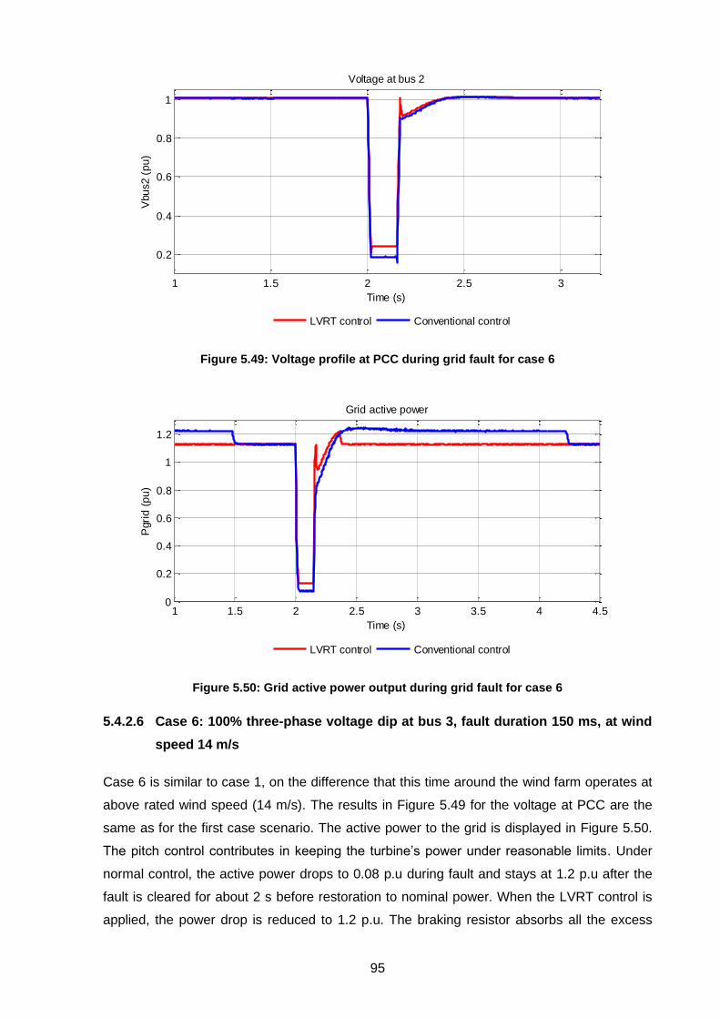
95
Figure 5.49: Voltage profile at PCC during grid fault for case 6
Figure 5.50: Grid active power output during grid fault for case 6
5.4.2.6 Case 6: 100% three-phase voltage dip at bus 3, fault duration 150 ms, at wind
speed 14 m/s
Case 6 is similar to case 1, on the difference that this time around the wind farm operates at
above rated wind speed (14 m/s). The results in Figure 5.49 for the voltage at PCC are the
same as for the first case scenario. The active power to the grid is displayed in Figure 5.50.
The pitch control contributes in keeping the turbine’s power under reasonable limits. Under
normal control, the active power drops to 0.08 p.u during fault and stays at 1.2 p.u after the
fault is cleared for about 2 s before restoration to nominal power. When the LVRT control is
applied, the power drop is reduced to 1.2 p.u. The braking resistor absorbs all the excess
1 1.5 2 2.5 3
0.2
0.4
0.6
0.8
1
Time (s)
Vbu
s2 (
pu
)
Voltage at bus 2
1 1.5 2 2.5 3 3.5 4 4.50
0.2
0.4
0.6
0.8
1
1.2
Grid active power
Time (s)
Pgri
d (
pu
)
LVRT control Conventional control
1 1.5 2 2.5 3
0.2
0.4
0.6
0.8
1
Time (s)
Vbu
s2 (
pu
)
Voltage at bus 2
1 1.5 2 2.5 3 3.5 4 4.50
0.2
0.4
0.6
0.8
1
1.2
Grid active power
Time (s)
Pgri
d (
pu
)
LVRT control Conventional control
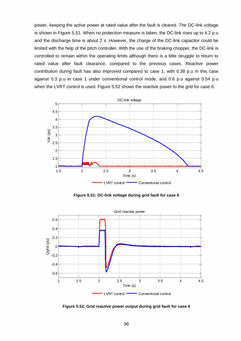
96
power, keeping the active power at rated value after the fault is cleared. The DC-link voltage
is shown in Figure 5.51. When no protection measure is taken, the DC-link rises up to 4.2 p.u
and the discharge time is about 2 s. However, the charge of the DC-link capacitor could be
limited with the help of the pitch controller. With the use of the braking chopper, the DC-link is
controlled to remain within the operating limits although there is a little struggle to return to
rated value after fault clearance, compared to the previous cases. Reactive power
contribution during fault has also improved compared to case 1, with 0.38 p.u in this case
against 0.3 p.u in case 1 under conventional control mode, and 0.6 p.u against 0.54 p.u
when the LVRT control is used. Figure 5.52 shows the reactive power to the grid for case 6.
Figure 5.51: DC-link voltage during grid fault for case 6
Figure 5.52: Grid reactive power output during grid fault for case 6
1.5 2 2.5 3 3.5 4 4.5
1
1.5
2
2.5
3
3.5
4
4.5
5
Time (s)
Vdc (
pu
)
DC-link voltage
1 1.5 2 2.5 3 3.5 4 4.5
-0.6
-0.4
-0.2
0
0.2
0.4
0.6
Grid reactive power
Time (s)
Qgri
d (
pu
)
LVRT control Conventional control
1.5 2 2.5 3 3.5 4 4.5
1
1.5
2
2.5
3
3.5
4
4.5
5
Time (s)
Vdc (
pu
)
DC-link voltage
1 1.5 2 2.5 3 3.5 4 4.5
-0.6
-0.4
-0.2
0
0.2
0.4
0.6
Grid reactive power
Time (s)
Qgri
d (
pu
)
LVRT control Conventional control

97
Figure 5.53: Voltage profile during fault at bus 3 for case 7
Figure 5.54: Voltage profile at PCC during grid fault for case 7
5.4.2.7 Case 7: 100% three-phase voltage dip at bus 3, fault duration 150 ms, at wind
speed 7 m/s
In this case, on the contrary to case 6, the LVRT capability of the wind turbine system is
tested with a grid fault occurring at low wind speed, here 7 m/s. The voltage profile at bus 3
showing the magnitude of the three phases is presented in Figure 5.53. As is in the previous
case, the magnitudes of the voltages drop to values close to 0 p.u during the fault. The PCC
voltage profiles for both the conventional and LVRT controls are also like in the previous
case. The PCC voltage in this case however restores pre-fault value after fault clearance
faster than in case 6. The grid active power is shown in Figure 5.55. the power supplied by
the wind farm is equal to 0.25 p.u of the rated power. During the fault this value drops to 0.08
1 1.5 2 2.5 3
-1
-0.5
0
0.5
1
Time (s)
Vbu
s3 (
pu
)
Three-phase voltages at bus 3
0 0.1 0.2 0.3 0.4 0.5 0.6 0.7 0.8 0.9 10
0.2
0.4
0.6
0.8
1
1 1.5 2 2.5 3
0.2
0.4
0.6
0.8
1
Time (s)
Vbu
s2 (
pu
)
Voltage at bus 2
1 1.5 2 2.5 30
0.2
0.4
0.6
0.8
1
Grid active power
Time (s)
Pgri
d (
pu
)
LVRT control Conventional control

98
p.u and 0.22 p.u using the conventional control and the LVRT control respectively, as in case
6. However, the overshoots after fault dismissal reach 1 p.u and last 50 ms on normal mode
against 0.84 p.u and 25 ms on LVRT control. For the DC-link voltage, its value reaches
around 1.76 p.u during fault under conventional control, then drops back to nominal value
almost immediately after the fault is cleared. The discharge time is almost inexistent in this
case since only 0.25 p.u active power is transferred to the grid at 7 m/s. Reactive power
contribution is the same as for case 6, however the negative peaks after fault removal are
reduced due to the short DC-link recovery time.
Figure 5.55: Grid active power output during grid fault for case 7
Figure 5.56: DC-link voltage during grid fault for case 7
1 1.5 2 2.5 3
0.2
0.4
0.6
0.8
1
Time (s)
Vbu
s2 (
pu
)
Voltage at bus 2
1 1.5 2 2.5 30
0.2
0.4
0.6
0.8
1
Grid active power
Time (s)
Pgri
d (
pu
)
LVRT control Conventional control
1 1.5 2 2.5 30.9
1
1.1
1.2
1.3
1.4
1.5
1.6
1.7
Time (s)
Vdc (
pu
)
DC-link voltage
1 1.5 2 2.5 3-0.4
-0.2
0
0.2
0.4
0.6
0.8Grid reactive power
Time (s)
Qgri
d (
pu
)
LVRT control Conventional control
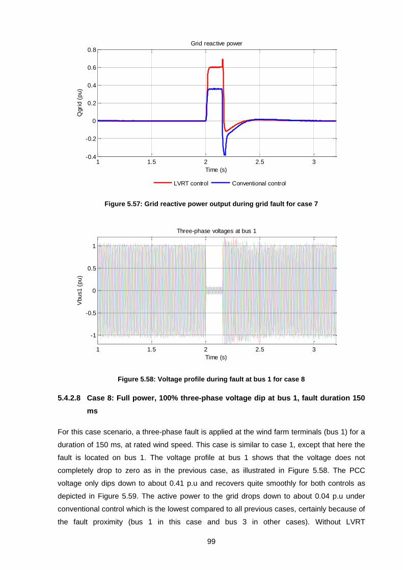
99
Figure 5.57: Grid reactive power output during grid fault for case 7
Figure 5.58: Voltage profile during fault at bus 1 for case 8
5.4.2.8 Case 8: Full power, 100% three-phase voltage dip at bus 1, fault duration 150
ms
For this case scenario, a three-phase fault is applied at the wind farm terminals (bus 1) for a
duration of 150 ms, at rated wind speed. This case is similar to case 1, except that here the
fault is located on bus 1. The voltage profile at bus 1 shows that the voltage does not
completely drop to zero as in the previous case, as illustrated in Figure 5.58. The PCC
voltage only dips down to about 0.41 p.u and recovers quite smoothly for both controls as
depicted in Figure 5.59. The active power to the grid drops down to about 0.04 p.u under
conventional control which is the lowest compared to all previous cases, certainly because of
the fault proximity (bus 1 in this case and bus 3 in other cases). Without LVRT
1 1.5 2 2.5 30.9
1
1.1
1.2
1.3
1.4
1.5
1.6
1.7
1.8
Time (s)
Vdc (
pu
)
DC-link voltage
1 1.5 2 2.5 3-0.4
-0.2
0
0.2
0.4
0.6
0.8Grid reactive power
Time (s)
Qgri
d (
pu
)
LVRT control Conventional control
1 1.5 2 2.5 3
-1
-0.5
0
0.5
1
Time (s)
Vbu
s1 (
pu
)
Three-phase voltages at bus 1
0 0.1 0.2 0.3 0.4 0.5 0.6 0.7 0.8 0.9 10
0.2
0.4
0.6
0.8
1

100
compensation, the DC-link voltage peaks at 3.7 p.u with a discharge time of about 0.6 s,
while the voltage is satisfactorily regulated with LVRT control. The active power and the DC-
link voltage are presented in Figure 5.60 and Figure 5.61 respectively. Finally, in Figure 5.62,
the reactive power is negative during the fault meaning that in this case, reactive power is
rather absorbed from the grid.
Figure 5.59: Voltage profile at PCC during grid fault for case 8
Figure 5.60: Grid active power output during grid fault for case 8
1 1.5 2 2.5 30.4
0.5
0.6
0.7
0.8
0.9
1
1.1
Time (s)
Vbu
s2 (
pu
)
Voltage at bus 2
1 1.5 2 2.5 30
0.2
0.4
0.6
0.8
1
1.2
Grid active power
Time (s)
Pgri
d (
pu
)
LVRT control Conventional control
1 1.5 2 2.5 30.4
0.5
0.6
0.7
0.8
0.9
1
1.1
Time (s)
Vbu
s2 (
pu
)
Voltage at bus 2
1 1.5 2 2.5 30
0.2
0.4
0.6
0.8
1
1.2
Grid active power
Time (s)
Pgri
d (
pu
)
LVRT control Conventional control

101
Figure 5.61: DC-link voltage during grid fault for case 8
Figure 5.62: Grid reactive power output during grid fault for case 8
Summary of the chapter
This chapter presented and discussed the simulation results of a grid connected PMSG wind
energy conversion system. The wind farm model aggregation techniques were used to
convert an individual 1.5 MW wind turbine into the 9 MW wind farm used in the simulations
studies. The electric power system used is a test platform developped on the MATLAB
Sympowersystems simulation tool. The WECS’s performance was first tested under normal
operating conditions. A varying wind speed profile was applied to the turbine system and
generator and grid side converter parameters were analyzed. The WPP was then tested
under grid fault conditions, where differents case scenarios were implemented with regards
1 1.5 2 2.5 3
1
1.5
2
2.5
3
3.5
4
Time (s)
Vdc (
pu
)
DC-link voltage
1 1.5 2 2.5 3-0.2
0
0.2
0.4
0.6
0.8Grid reactive power
Time (s)
Qgri
d (
pu
)
LVRT control Conventional control
1 1.5 2 2.5 3
1
1.5
2
2.5
3
3.5
4
Time (s)
Vdc (
pu
)
DC-link voltage
1 1.5 2 2.5 3-0.2
0
0.2
0.4
0.6
0.8Grid reactive power
Time (s)
Qgri
d (
pu
)
LVRT control Conventional control

102
to the fault type, the fault depth, the fault duration and the fault position. The results were
compared on the basis that faults compensation methods were employed in addition to the
conventional controller or not during grid different faults.

103
CHAPTER SIX
6 CONCLUSIONS AND RECOMMENDATIONS
This thesis investigated the capability of a wind energy conversion system in remaining
connected to the electrical network during grid disturbances, in this case voltage drop, as per
specified by the grid code FRT requirement presented in section 3.8 of this document. The
installation of large capacity wind power plants as an attempt to reduce the global carbon
emissions has emphasized the urge for system operators to ensure that wind farms
connected to the transmission and distribution networks comply with certain requirements,
for smooth, safe and reliable grid operation. In fact, a loss in generation capacity due to a
large scale WPP disconnection as a result of a grid voltage sag may lead to a succession of
production losses which could further cause a partial or sometimes complete power system
shutdown. This situation is clearly undesirable and therefore should be absolutely avoided.
In this study, a grid connected PMSG WECS was tested with regards to its ability to ride
through a low voltage inception at grid level. Different case scenarios were investigated.
From the simulation results it can be concluded that:
• The system shows great stability under varying wind speed conditions. MPPT is
successfully achieved through OTC on the generator side, while DC-link regulation and
unity power factor operation objectives are met on the grid side.
• The braking chopper circuit manages to keep the DC-link voltage at an acceptable level
during different grid sag conditions, ensuring the safety of the power converters.
• The braking chopper only regulates the DC-link voltage and does not improve the PCC
voltage drop during the fault. However, there is a faster and smoother recovery to pre-
fault value after fault dismissal.
• Reactive current injection can considerably reduce the power through the DC-link by
increasing the voltage at the connection point during a grid fault. In most cases, this is
not sufficient in keeping the DC-link voltage below the maximum allowable limit. The
braking chopper therefore overtakes the protection duty.
• The grid side converter successfully supplies reactive current to support the grid voltage
during fault, according to the reactive power support requirement described in figure 3.9
of section 3.1.5.
• When the fault occurs at the wind farm’s terminals, reactive power is rather absorbed
from the grid and the PCC voltage is not supported.

104
The following suggestions are proposed for future investigations:
• The study could also be conducted on a larger scale using an IEEE 14-bus test sytem or
even a portion of the South African network as test benchmark and other grid code
requirements could be investigated.
• An experimental approach of the study could be implemented through real time
simulations and laboratory scale work.
• Interaction between individual wind turbines in a WPP using a detailed wind farm model
in the case of internal abnormalities.
• Reactive power supervisory control of grid connected renewable energy systems during
grid faults.
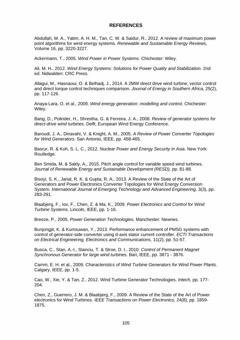
105
REFERENCES
Abdullah, M. A., Yatim, A. H. M., Tan, C. W. & Saidur, R., 2012. A review of maximum power point algorithms for wind energy systems. Renewable and Sustainable Energy Reviews, Volume 16, pp. 3220-3227.
Ackermann, T., 2005. Wind Power in Power Systems. Chichester: Wiley.
Ali, M. H., 2012. Wind Energy Systems: Solutions for Power Quality and Stabilization. 2nd ed. Nidwalden: CRC Press.
Allagui, M., Hasnaoui, O. & Belhadj, J., 2014. A 2MW direct drive wind turbine; vector control and direct torque control techniques comparison. Journal of Energy in Southern Africa, 25(2), pp. 117-126.
Anaya-Lara, O. et al., 2009. Wind energy generation: modelling and control. Chichester: Wiley.
Bang, D., Polinder, H., Shrestha, G. & Ferreira, J. A., 2008. Review of generator systems for direct-drive wind turbines. Delft, European Wind Energy Conference.
Baroudi, J. A., Dinavahi, V. & Knight, A. M., 2005. A Review of Power Converter Topologies for Wind Generators. San Antonio, IEEE, pp. 458-465.
Basrur, R. & Koh, S. L. C., 2012. Nuclear Power and Energy Security in Asia. New York: Routledge.
Ben Smida, M. & Sakly, A., 2015. Pitch angle control for variable speed wind turbines. Journal of Renewable Energy and Sustainable Development (RESD), pp. 81-88.
Bisoyi, S. K., Jarial, R. K. & Gupta, R. A., 2013. A Review of the State of the Art of Generators and Power Electronics Converter Topologies for Wind Energy Conversion System. International Journal of Emerging Technology and Advanced Engineering, 3(3), pp. 283-291.
Blaabjerg, F., Iov, F., Chen, Z. & Ma, K., 2009. Power Electronics and Control for Wind Turbine Systems. Lincoln, IEEE, pp. 1-16.
Breeze, P., 2005. Power Generation Technologies. Manchester: Newnes.
Bunjongjit, K. & Kumsuwan, Y., 2013. Performance enhancement of PMSG systems with control of generator-side converter using d-axis stator current controller. ECTI Transactions on Electrical Engineering, Electronics and Communications, 11(2), pp. 51-57.
Busca, C., Stan, A.-I., Stanciu, T. & Stroe, D. I., 2010. Control of Permanent Magnet Synchronous Generator for large wind turbines. Bari, IEEE, pp. 3871 - 3876.
Camm, E. H. et al., 2009. Characteristics of Wind Turbine Generators for Wind Power Plants. Calgary, IEEE, pp. 1-5.
Cao, W., Xie, Y. & Tan, Z., 2012. Wind Turbine Generator Technologies. Intech, pp. 177-204.
Chen, Z., Guerrero, J. M. & Blaabjerg, F., 2009. A Review of the State of the Art of Power electronics for Wind Turbines. IEEE Transactions on Power Electronics, 24(8), pp. 1859-1875.

106
Chowdhury, M. M. et al., 2012. Enhanced control of a direct drive grid connected wind energy system with STATCOM. Bali, IEEE, pp. 1-6.
Conroy, J. F. & Watson, R., 2007. Low-voltage ride-through of a full converter wind turbine with permanent magnet generator. Renewable Power Generation, IET, 1(3), pp. 182-189.
Craddock, D., 2008. Renewable energy made easy: free energy from solar, wind, hydropower, and other alternative energy sources. Ocala: Atlantic Publishing Group, Inc.
de Alegria, I. M. et al., 2007. Connection requirements for wind farms: A survey on technical requirements and regulations. Renewable and Sustainable Energies Reviews, Issue 11, pp. 1858-1872.
de Freitas, T. R. S., Menegaz, P. J. M. & Simonetti, D. S. L., 2011. Converter Topologies for Permanent Magnetic Synchronous Generator on Wind Energy Conversion System. Praiamar, IEEE, pp. 936-942.
Debnath, S. & Saeedifard, M., 2013. A New hybrid modular multilevel converter for grid connection of large wind turbines. IEEE Transactions on Sustainable Energy, 4(4), pp. 1051-1064.
Dong, S., Li, H. & Wang, Y., 2012. Low voltage ride through capability enhancement of PMSG-based wind turbine. Hangzhou, IET, pp. 1-5.
Earnest, J., 2015. Wind power technology. 2nd ed. Delhi: PHI.
Earnest, J. & Wizelius, T., 2011. Wind power plants and project development. New Delhi: PHI Learning Private Limited.
Florescu, A. et al., 2010. Advantages, limitations and disadvantages of z-source inverter. Sinaia, IEEE, pp. 483-486.
Freire, N. M. A., 2013. Fault-tolerant permanent magnet synchronous generator drives for wind turbine applications, Coimbra: s.n.
Greencape, 2015. Renewable energy, green cape intelligence report 2015, s.l.: s.n.
Gupta, A., Jain, D. K. & Dahiya, S., 2012. Some Investigations on Recent Advances in Wind Energy Conversion Systems. Coimbatore, IACSIT Press, pp. 47-52.
GWEC, 2015. Global wind report: annual market update 2014. [Online] Available at: https://gwec.net/publications/global-wind-report-2/global-wind-report-2014-annual-market-update/ [Accessed 27 April 2015].
Hansen, A. D. & Michalke, G., 2007. Fault ride-through capability of DFIG wind turbines. Renewable Energy, 32(9), pp. 1594-1610.
Hansen, A. D. & Michalke, G., 2009. Multi-pole permanent magnet synchronous generator wind turbines grid support capability in uninterrupted operation during grid faults. IET Renewable Power Generation, 3(3), pp. 333-348.
Hansen, M. O. L., 2008. Aerodynamics of wind turbines. 2nd ed. London: Earthscan.
Hau, E., 2013. Wind Turbines: Fundamentals, Technologies, Applications, Economics. 3rd ed. Berlin: Springer-Verlag.

107
Heir, S., 2014. Grid integration of wind energy conversion systems. 3rd edition ed. Chichester: John Wiley & Sons.
Heng, N., Jiao, L., Peng, Z. & Yikang, H., 2008. Improved control strategy of an active crowbar for directly-driven PM wind generation system under grid voltage dips. Wuhan, IEEE, pp. 2294-2298.
Heydari, M. & Smedley, K., 2015. Comparison of maximum power point tracking methods for medium to high power wind energy systems. Zahedan, IEEE.
Huang, N., 2013. Simulation of power control of wind turbine permanent magnet synchronous generator system, Milwaukee: epublications.
Hu, J. et al., 2010. A novel control strategy for Doubly Fed Induction Generator and Permanent Magnet Synchronous Generator during voltage dips. Christchurch, IEEE, pp. 1-6.
Ibrahim, R. A., Hamad, M. S., Dessouky, Y. G. & Williams, B. W., 2012. A review on recent low voltage ride-through solutions for PMSG wind turbines. Sorrento, IEEE, pp. 265-270.
IEA, 2012. World Energy Outlook 2012. [Online] Available at: http://www.iea.org/publications/freepublications/publication/WEO2012_free.pdf [Accessed 30 April 2014].
Jamil, M., Gupta, R. & Singh, M., 2012. A review of power converter topology used with PMSG based wind power generation. Murthal, IEEE, pp. 1-6.
Jash, K., Saha, P. K. & Panda, G. K., 2013. Vector control of permanent magnet synchronous motor based on sinusoidal pulse width modulated inverter with proportional integral controller. Journal of Engineering Research and Applications, 3(5), pp. 913-917.
Kasem Alaboudy, A. H., Daoud, A. A., Desouky, S. S. & Salem, A. A., 2013. Converter controls and flicker study of PMSG-based grid connected wind turbines. Ain Shams Engineering Journal, Volume 4, pp. 75-91.
Kesraoui, M., Bencherouda, O. & Mesbahi, Z., 2010. Power control of PMSG based wind turbine system above rated wind speed. Sousse, IREC, pp. 133-140.
Khater, F. & Omar, A., 2013. A Review of Direct Driven PMSG for Wind Energy Systems. Journal of Energy and Power Engineering, Volume 7, pp. 1592-1603.
Kilk, A., 2007. Low-speed permanent-magnet synchronous generator for small-scale wind power applications. Oilshale, 24(2), pp. 318-331.
Kim, H. S. & Lu, D. D.-C., 2010. Review on wind turbine generators and power electronic converters with the grid-connection issues. Christchurch, IEEE, pp. 1-6.
Koc, E., 2010. Modelling and Investigation of Fault Ride Through Capability of Variable Speed Wind Turbines, Ankara: Middle East Technical University.
Kundur, P. S., 1994. Power system stability and control. New York: McGraw-Hill Professional.
Leao, R. P. S. et al., 2010. The Implementation of the Low Voltage Ride-Through Curve on the Protection System of a Wind Power Plant. Las Palmas de Gran Canaria, European Association for the Development of Renewable Energies, Environment and Power Quality.
Li, H. & Chen, Z., 2008. Overview of Different Wind Generator Systems and their Comparisons. IET Renewable Power Generation, 2(2), pp. 123-138.

108
Madani, N., 2011. Design of a permanent magnet synchronous generator for vertical axis wind turbine, Stockholm: Royal Institute of Technology.
Manwell, J., Mcgowan, J. & Rogers, A., 2009. Wind energy explained: theory, design and application. 2nd ed. Chichester: Wiley.
Marrone, C. A. Q., 2014. Challenges for the integration of wind park clusters into power grids: Approach and methodology for the integration and dispatch of wind park clusters into the power grids, s.l.: BoD.
Mchunu, T. & Khoza, T., 2013. Grid connection code for renewable power plants South Africa. East London, AMEU.
Melicio, R., Mendes, V. M. F. & Catalao, J. P. S., 2010. Modeling, control and simulation of full-power converter wind turbines equipped with permanent magnet synchronous generator. International Review of Electrical Engineering, 5(2), pp. 397-408.
Mittal, R., Sandhu, K. & Jain, D., 2010. An Overview of Some Important Issues Related to Wind Energy Conversion System (WECS). International Journal of Environmental Science and Development, 1(4), pp. 351-363.
Mittal, R., Sandhu, K. S. & Jain, D. K., 2009. Low Voltage Ride-Through (LVRT) of Grid Interfaced Wind Driven PMSG. ARPN Journal of Engineering and Applied Sciences, 4(5), pp. 73-83.
Mohseni, M. & Islam, S. M., 2011. Comparing technical connection requirements for large wind power plants. San Diego, IEEE, pp. 1-8.
Mohseni, M. & Islam, S. M., 2012. Review of international grid codes for wind power integration: Diversity, technology and a case for global standard. Renewable and Sustainable Energies Reviews, Issue 16, pp. 3876-3890.
Munteanu, I., Bratcu, A. I., Cutululis, N.-A. & Ceanga, E., 2008. Optimal control of wind energy systems: Towards a global approach. London: Springer-Verlag.
Nasiri, M., Milimonfared, J. & Fathi, S. H., 2015. A review of low-voltage ride-through methods for permanent magnet synchronous generator based wind turbines. Renewable and Sustainable Energy Reviews , Volume 47, pp. 399-415.
Nguyen, T. H. & Lee, D.-C., 2010. Ride-through technique for PMSG wind turbines using energy storage systems. Journal of Power Electronics, 10(6), pp. 733-738.
Nguyen, T. H. & Lee, D.-C., 2013. Advanced Fault Ride-Through Technique for PMSG Wind Turbine Systems Using Line-Side Converter as STATCOM. IEEE Transactions on Industrial Electronics, 60(7), pp. 2842 - 2850.
Pandu Ranga, R. G. & Vijaya, K. M., 2013. Implementation of matrix converter based PMSG for wind energy conversion system. Coimbatore, IEEE, pp. 115-120.
Patel, M. R., 2006. Wind and solar power systems: design, analysis, and operation. 2nd ed. Nidwalden: CRC Press.
Peng, F. Z., 2002. Z-source inverter. Pittsburgh, IEEE, pp. 775-781.
Perelmuter, V. M., 2013. Electrotechnical Systems: simulation with simulink and simpowersystems. Boca Raton: CRC Press.
109
Polinder, H., Bang, D.-J., Li, H. & Chen, Z., 2007. Concept Report on Generator Topologies, Mechanical & Electromagnetic Optimization, s.l.: s.n.
Prerna, B. & Jagdeesh Kumar, P. S., 2013. Study of Power Converter Topology used for Renewable Energy Resources using Wind. International Journal of Emerging Research in Management & Technology, 2(12), pp. 2278-9359.
Qiao, W., Harley, R. G. & Venayagamoorthy, G. K., 2007. Dynamic Modeling of Wind Farms with Fixed-Speed Wind Turbine Generators. Tampa, IEEE.
Qiu, Z., Zhou, K. & Li, Y., 2011. Modeling and control of diode rectifier fed PMSG based wind turbine. Weihai, IEEE, pp. 1384-1388.
Quang, N. P. & Dittrich, J. A., 2008. Vector control of three-phase AC machines. Berlin: Springer.
Raphael, S. & Massoud, A., 2011. Unified power flow controller for low voltage ride through capability of wind-based renewable energy grid-connected systems. Sousse, IEEE, pp. 1-6.
Rekioua, D., 2014. Wind power electric systems: modeling, simulation and control. New York: Springer.
Ren21, 2015. Renawables 2015: global status report. [Online] Available at: https://www.ren21.net/wp-content/uploads/2019/05/GSR2015_Full-Report_English.pdf [Accessed 27 April 2015].
Rolan, A. et al., 2009. Modeling of a variable speed wind turbine with a permanent magnet synchronous generator. Seoul, IEEE, pp. 734-739.
Rosyadi, M., Muyeen, S. M., Takahashi, R. & Tamura, J., 2011. Low voltage ride-through capability improvement of wind farms using variable speed permanent magnet wind generator. Beijing, IEEE, pp. 1-6.
Sanchez, A. G., Molina, M. G. & Rizzato Lede, A. M., 2012. Dynamic model of wind energy conversion systems with PMSG-based variable-speed wind turbines for power system studies. International journal of Hydrogen Energy, Volume 37, pp. 10064-10069.
Shuju, H., Jianlin, L. & Honghua, X., 2008. Modeling on converter of direct-driven WECS and its characteristics during voltage sags. Chengdu, IEEE, pp. 1-5.
Soriano, L. A., Yu, W. & Rubio, J. d. J., 2013. Modeling and control of wind turbine. Mathematical Problems in Engineering, Volume 2013, pp. 1-13.
Sourkounis, C. & Tourou, P., 2013. Grid Code Requirements for Wind Power Integration in Europe. Limasol, Hindawi Publishing Corporation, pp. 1-9.
Tong, W., 2010. Wind power generation and wind turbine design. Southampton: WIT Press.
Tsili, M., Patsiouras, C. & Papathanassiou, S., 2009. A review of grid code technical requirements for wind farms. IET Renewable Power Generation, 3(3), pp. 308-332.
Vilathgamuwa, D. M., Wang, X., Tseng, K. J. & Gajanayake, C. J., 2008. Z-source inverter based grid-interface for variable-speed wind turbine generators. Rhodes, IEEE, pp. 4545-4550.
Vittal, V. & Ayyanar, R., 2013. Grid integration and dynamic impact of wind energy. New York: Springer.
110
Wagner, H.-J. & Mathur, J., 2009. Introduction to wind energy systems: basics, technology and operation. Berlin: Springer.
Wenming, G., Yun, W., Shuju, H. & Honghua, X., 2011. A survey on recent low voltage ride-through solutions of large scale wind farm. Wuhan, IEEE, pp. 1-5.
Wenske, J., 2011. Wind Energy Report Germany 2011 Special Report: Direct Drives and drive-train development trands, s.l.: Siemens Press Picture.
Writer, S., 2015. BusinessTech. [Online] Available at: http://businesstech.co.za/news/energy/93743/south-africas-biggest-wind-farms-vs-the-world/ [Accessed 10 December 2015].
Wu, B., Lang, Y., Zargari, N. & Kouro, S., 2011. Power conversion and control of wind energy systems. New Jersey: Wiley.
Yamarasu, V. et al., 2015. High-power wind energy conversion systems: state-of-the-art and emerging technologies. Proceedings of the IEEE, 103(5), pp. 740-788.
Yang, G. & Li, H., 2009. Application of a matrix converter for PMSG wind turbine generation system. Capri, IEEE, pp. 619-623.
Yang, X.-p., Duan, X.-f., Feng, F. & Tian, L.-l., 2009. Low voltage ride-through of directly driven wind turbie with permanent magnet synchronous genenrator. Wuhan, IEEE, pp. 1-5.
Yan, L. et al., 2011. Study on LVRT capability of D-PMSG based wind turbine. s.l., s.n.
Zeng, Q. & Chang, L., 2005. Study of advanced control strategies for three-phase grid-connecter PWM inverters for distributed generation. Toronto, IEEE, pp. 1311-1316.

111
APPENDICES
6.1 Appendix A: System parameters
Table A.1: Individual wind turbine parameters (Nasiri, et al., 2015)
Parameters Values
Rated power 1.5 MW
Air density 1.225 kg/m3
Blade radius 35.25 m
Maximum power coefficient 0.48
Optimal tip speed ratio 8.1
Rated wind speed 11 m/s
Total moment of inertia 4872000 kg/m2
Damping coefficient 200 Nms/rad
Table A.2: Generator parameters (Nasiri, et al., 2015)
Parameter Value
Rated power 1.5 MW
Rated voltage 690 V
Rated flux 7.0172 Wb
Stator resistance 3.17 mΩ
Stator inductance 3.07 mH
Number of pole pairs 40
Table A.3: DC-link parameters (Nasiri, et al., 2015)
Parameter Value
DC-link voltage 1500 V
DC-link capacitance 0.023 F
Switching frequency 5000 Hz

112
6.2 Appendix B: System simulation model

113
Figure B.6.1: Electric power system model

114
Figure B.6.2: Complete model of the PMSG wind energy conversion system
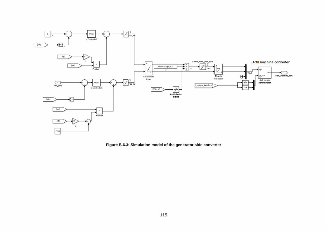
115
Figure B.6.3: Simulation model of the generator side converter

116
Figure B.6.4: Simulation model of the grid side converter