Fault detection based on time series modeling andmultivariate statistical process control

A. Sanchez-Fernandeza, F.J. Baldanb, G.I. Sainz-Palmeroa, J.M. Benıtezb,M.J. Fuentea,∗

aDepartment of System Engineering and Automatic Control, EII, University of Valladolid,Valladolid, Spain

bDepartment of Computer Science and Artificial Intelligence, University of Granada,Granada, Spain

Abstract

Monitoring complex industrial plants is a very important task in order to en-sure the management, reliability, safety and maintenance of the desired productquality. Early detection of abnormal events allows actions to prevent more seri-ous consequences, improve the system’s performance and reduce manufacturingcosts. In this work, a new methodology for fault detection is introduced, basedon time series models and statistical process control (MSPC). The proposal ex-plicitly accounts for both dynamic and non-linearity properties of the system.A dynamic feature selection is carried out to interpret the dynamic relations bycharacterizing the auto- and cross-correlations for every variable. After that,a time-series based model framework is used to obtain and validate the bestdescriptive model of the plant (either linear o non-linear). Fault detection isbased on finding anomalies in the temporal residual signals obtained from themodels by univariate and multivariate statistical process control charts. Finally,the performance of the method is validated on two benchmarks, a wastewatertreatment plant and the Tennessee Eastman Plant. A comparison with otherclassical methods clearly demonstrates the over performance and feasibility ofthe proposed monitoring scheme.

Keywords: Fault detection, Dynamic feature selection, Time-series modeling,Statistical process control charts

∗Corresponding author, M.J. Fuente. Department of Systems Engineering and AutomaticControl, EII, C/ Paseo del Cauce N.59, Post code: 47011, University of Valladolid, Valladolid,Spain, Tlf: +34 983 42 33 55

Email addresses: alvar.sanchez@uva.es (A. Sanchez-Fernandez),fjbaldan@decsai.ugr.es (F.J. Baldan), gresai@eii.uva.es (G.I. Sainz-Palmero),j.m.benitez@decsai.ugr.es (J.M. Benıtez), mjfuente@eii.uva.es (M.J. Fuente )

Preprint submitted to Chemometrics and Intelligent Laboratory Systems July 24, 2018

1. INTRODUCTION

The increasing complexity of modern industrial processes brings with it anincrease in the importance of process monitoring to ensure plant safety andproduct quality [1]. Early detection of abnormal events allows actions to pre-vent more serious consequences, improve the system’s behaviour and reducemaintenance and operation costs. The main objective of anomaly, or fault, de-tection is to identify any abnormal event indicating a distance from the processbehaviour as compared to its normal behaviour. In other words, an anomalyoccurs when the system deviates significantly from its normal situation duringthe on-line operation. The second goal is fault diagnosis (or isolation), whichdetermines the root cause of the detected anomaly.

Process monitoring can generally be divided into three categories: model-based methods, knowledge-based methods, and data-based methods [2–4]. Thefirst category is also called analytical redundancy (AR), in which an explicitmodel is used. Unusual events are detected by referencing the measured processbehaviour against the model. However, as modern industrial processes becomemore and more complex it is difficult and time consuming to develop an accuratemodel that characterizes all the physical and chemical phenomena occurringin industrial processes. Fault detection using knowledge-based techniques isusually a heuristic process based on the available knowledge of the system’sbehaviour and the experience of expert plant operators. However, the creationof the process knowledge base is always a time consuming and difficult operation,requiring the long-term accumulation of expert knowledge and experience.

Furthermore, data-based anomaly-detection methods rely on the availabilityof historical data of the inspected system under normal operation mode. Thesemethods have become more and more popular in recent years, especially incomplex industrial processes, where models and knowledge are difficult to obtainin practice and where, because of the wide utilization of distributed controlsystems, large amounts of data have been collected. Such data contain the mostprocess information and can be used for modelling and monitoring the process.In particular, multivariate statistical process control (MSPC), such as PrincipalComponent Analysis (PCA), Partial Least Squares (PLS), etc. have been usedto monitor different industrial processes [5, 6].

Industrial plants are normally non-linear and dynamic. To deal with thedynamic property in the processes, dynamic PCA utilizing an augmented ma-trix with time-lagged variables, which models the auto-correlation and cross-correlation among data samples, was proposed in [7] and used in different ap-plications [8, 9]. Canonical variate analysis (CVA) has also been proposed fordynamic process monitoring [10], where both past data and future measure-ments are used to estimate the process state space model and build a faultdetection scheme. However, there are some limitations for these techniques,as the high dimensionality of the augmented matrix, which cannot be appliedto monitoring a large number of auto-correlated, cross-correlated and collinearvariables.

Some process variables can affect other variables with a time-delay [11];

2

a time-delayed process variable might have a stronger relationship with othervariables (delayed or not) than the non-delayed one. So, high cross-correlationamong process variables with different time-delays is possible, and it is difficultto select both auto-correlation and cross-correlation together, i.e., dynamic fea-tures, for every process variable. However, it is expected that a proper selectionwill improve the monitoring scheme’s behaviour.

To solve the problem of non-linearity, some extensions of non-linear PCAhave been reported in the literature, such as [12], which develops a non-linearPCA based on autoassociative neural networks; while, more recently, [13] presentsa similar idea, but using neural networks called invariant autoencoders (AE),equivalent to non-linear PCA, to extract a robust and non-linear representationof the process data. However, these methods usually require more computationand inevitably lead to the convergence to the local minimum during the net-work training. In addition, the number of principal components (PCs) must bespecified in advance before training the neural networks.

A different idea is proposed in [14] and this is called Kernel PCA (KPCA),where non-linear data in the input space is transformed into linear data in ahigh dimensional feature space, through a non-linear mapping, a kernel trick,to calculate the principal components in the feature space [15]. However, thedrawback of KPCA is that the computation time may increase with the numberof samples, and the data pattern in the feature space is rather hard to interpretin the input space; so it is hard to identify the variables causing the fault. Inaddition, the fault detection of KPCA is very sensitive to the parameters ofthe kernel function used to implement it, especially for the radial basis functionor the Gaussian kernel, the most commonly used one. Finally, there is notheoretical framework for specifying the optimal value for those parameters.

Motivated by the above considerations, the objective of this paper is topresent a dynamic and non-linear fault detection and diagnosis methodology,that explicitly accounts for the dynamic relations in the process through dy-namic feature selection, and for the non-linear relationship between the processvariables through a time-series based model, capturing both the non-linear andthe dynamic correlation in the process. Thus, the residuals, which are the dif-ference between the process measurements and the output of the time-seriesmodel, can be monitored by conventional SPC charts, because the time-seriesmodel is used to remove the non-linear and the dynamic characteristics of theprocess. Therefore, the main objective of this paper is to combine the advan-tages of the SPC monitoring scheme and time-series modelling to enhance theperformance of the monitoring scheme and widen its applicability in practicefor complex and large-scale industrial processes.

The proposal works as follows: first, a dynamic feature selection methodto characterize the dynamic relations of every process variable is carried out;then, a time series model is developed for every variable taking into accountthe features previously obtained; the residuals are then processed by differentSPC charts. Every residual is processed by univariate statistics, the EWMAchart [16, 17], to detect and diagnose faults when one of the residuals exceedsits control limits. As this frequently happens, the systems have a very large

3

number of variables, so it is better to process all the variables together to obtaina unique statistic to check whether there is a fault in the system or not. In thispaper, the residuals are also processed by the well-known PCA algorithm, usingthe classical Hotelling’s and SPE statistics to detect the faults.

The major contributions of the current work can be summarized as: (1)proposing a general methodology to monitor dynamic and non-linear complexprocess; (2) proposing a dynamic feature characterization for the dynamic pro-cesses; and (3) ensuring consistent monitoring performance compared to otherfault detection methods driven by data.

The rest of this paper is organized as follows: Section 2 briefly reviews thetheoretical concepts used related to the dynamic feature selection, the statisticalprocess control and the time series modelling; Section 3 presents an explanationof the proposed approach; and Section 4 outlines the application of the proposedmethodology to two complex systems: a waste water treatment plant and theTennessee Eastman plant. Finally, Section 5 reviews the main points discussedin this work and concludes the study.

2. THEORY

In order to carry out this proposal, it is necessary to identify m differentmodels, for a system with m sensors measuring m system variables, from themeasurement data recorded by the sensors. In particular, for each system vari-able xi, i = 1, ...,m, we are looking for a forecasting time-series model fi basedon a subset or a transformation of the other variables which are best able topredict this variable. At the same time, the aim is to find nominal systemmodels with dynamic dependencies, i.e., where a variable might have influenceon a target in several time steps in the future (but not immediately). Thus,it is aiming for a vectorized time-series model, where the prediction model fifor each variable xi, i = 1, ...,m includes the necessary time-lags on a subset ofother variables, which are the best to explain this variable. So, the data setcontaining the variable to be modelled is spanned to include lags along the moriginal non-delayed variables as inputs to the model.

xi(t) = [x1(t), ..., x1(t− k1), xi(t− 1), ...xi(t− ki), ..., xm(t), ...xm(t− km)] (1)

where {k1, k2, ..., km} ⊆ {0, ..., L}, thus allowing variables without lags to par-ticipate in the model definition. L denotes the maximal lags and will be set to aconcrete value calculated with a dynamic feature selection. In this way, modelsare potentially obtained where no lags, different lags from the same variable, ordifferent lags from different variables, may appear as inputs.

2.1. Dynamic feature selection

The interaction among different measured variables might be more appropri-ately represented on the basis of different time-delays. In order to model everyvariable, it is necessary to know which are the best relations for using. So a

4

dynamic feature selection concerning auto- and cross-correlation with differenttime-delays is carried out. First, the matrix X (n samples × m variables), withthe original variables in normal operation conditions, is augmented, taking foreach observation its previous L observations and stacking the data matrix inthe following manner:

Xa = [Xt|Xt−1| . . . |Xt−L] (2)

where the operator | is the matrix concatenation operator, Xa ∈ <(n−L)×(m(L+1))

is the augmented matrix, Xt is the data matrix X at the time instant t andXt−L at the time instant t− L, that is, with a delay of L time samples.

To implement the dynamic feature selection, the relationship between twovariables xit and xjl at two different time instants is calculated as the absolutevalue of the correlation coefficient :

<i(xit,x

jl) =

∣∣∣xiTt xjl /‖xit‖‖xjl ‖∣∣∣ (3)

where i, j = 1, ...,m and t, l = 1, ..., L. This coefficient is a direct measure of thecorrelation between variables and, after the calculation of vector <i for the i-thvariable, the dynamic feature selection is carried out by selecting the variablesin matrix Xa with high correlation values, i.e., <i > δi, are selected as inputs tomodel the variable xi, with δi being a cut off parameter for each variable thatdepends on the correlation present in the system.

Other method used for the dynamic feature selection is Dynamic PartialLeast Squares (DPLS) [18]. It is a well known method to reduce the dimen-sionality of a system and it searches for a new feature set composed of linearcombinations of the original ones. This method then adjusts a linear modelusing least squares over these new discovered features.

X = TPT + E (4)

Y = TQT + F (5)

where X is the predictor matrix (n × m), Y is the response matrix (n × p),T is the first k terms of the latent variables or the score vectors, P and Q,respectively, are the loading vectors of the data matrices X and Y, and Eand F are the residual terms of PLS. In general, each score is extracted throughdeflating X and Y by the well known algorithm of the non-linear iterative partialleast squares (NIPALS) until all variance in the data structure is explained [19].These score vectors are calculated as:

T = XR (6)

This matrix R = W(PTW)−1 is very useful to show which variables in Xare most related to the model response Y. The way in which this method canperform the regression is:

Y = XBPLS + F, BPLS = RQT (7)

5

So in this case, the augmented matrix Xa (eq. 2) is constructed and a PLSregression model is calculated, taking each of the system variables, Y = xi,i = 1, ...m as output variable and the matrix Xa as the predictor, withoutthe corresponding i-th variable that is being modelled. The dynamic featureselection is carried out by selecting the variables in matrix Xa with high absolutevalue of regression coefficients, i.e., high values of the vector BPLS.

A third way for the dynamic feature selection to be done is by combiningboth methods, i.e., first to do a dynamic feature selection with the correlationcoefficient between variables and, after that, refine the selection using the PLSmethod. So, the variables and their delays with bigger correlation coefficientare chosen first, and these variables are arranged in a data matrix Xi, one foreach variable in the system, i = 1, ...m. After that, a PLS regression model isobtained for the variable i-th, while the variables with bigger absolute valuesof the corresponding regression coefficients, BPLSi, are chosen as final inputvariables.

For the special case of ARIMA models, where the data of each variable aremodelled using only the delayed information from each respective variable, thedynamic feature selection is done using the Autocorrelation Function (ACF)and Partial Autocorrelation Function (PACF) [20].

2.2. Time series modelling

Many methods have been developed to analyze and forecast time-series [21],making the choice of an appropriate method an important task. A brief sum-mary of time-series models is presented:

Autoregressive Integrated Moving Average. The three univariate time-seriesmodels which have been widely applied are the autoregressive (AR), the mov-ing average (MA) and the autoregressive and moving average models (ARMA),and when the system is not stationary, the ARIMA model ([20, 22]). Whena time-series exhibits seasonality, a SARIMA model can be used to measurethe seasonal effect or eliminate seasonality. In this time-series model (ARIMA),a variable is modelled through its own lags, and does not explicitly use theinformation contained in other related time-series. In industrial processes thevariables are not independent and besides the autocorrelation of each variable,there exists high a cross-correlation among different process variables with differ-ent time-delays. To capture the relationships between them, time-series modelswith exogenous or input variables can be used, so the autoregressive moving av-erage model with external inputs (ARMAX) and its variants (ARX, ARIMAX,SARIMAX,...) can be suitable.

Neural Networks. Neural networks are a useful non-linear modelling tech-nique [23], especially the Multilayer Perceptions (MLP) neural networks, whichare capable of approximating, to arbitrary accuracy, any continuous functionas long as they contain enough hidden units [24]. Their attractive propertieshave led to the rise of several types of NNs and applications in the literature indifferent fields ([25–27]).

Support vector regression. Support vector machine (SVM) analysis is a pop-ular machine learning tool for classification and regression, first identified by

6

[28]. It supposes a training dataset (xi, yi) i = 1, ...N ⊂ X ×R where X denotesthe space of input patterns. The goal is to find a function f(x) that has at mostε deviation from the actually obtained targets yi for all training data and, atthe same time, is as smooth as possible. This is known as ε- SV regression:

f(x) = 〈w, x〉+ b (8)

with w ∈ X , b ∈ R. When the problem is non-linear, an SVM can be used as anon-linear regression function by using the kernel trick to map the input featurespace to a higher dimensional feature space, where a linear decision function isconstructed. ([29–31])

2.3. Statistical process control techniques

The aim of Statistic Process control (SPC) is to monitor a process to detectabnormal behaviour. In order to detect faults, the statistical control charts (alsoreferred to as monitoring charts) are used [32]. They present a value over timeand some thresholds that must not be surpassed in normal operating conditions.So, these control charts are crucial in detecting whether a process is still workingunder normal operating conditions (usually termed in-control) or not (out-of-control). Within this framework, different control charts have been developedto monitor the system over time, including [33]:

• Shewhart control chart [34]: this represents the time evolution of themean of a variable with upper and lower limits. If one of these thresholdsis exceeded, a fault is detected. To avoid false alarms, it is usual to requirea certain number of consecutive instants with abnormal values to activatethe fault alarm.

• Cumulative Sum (CUSUM) charts [35, 36]: here the method represents thecumulative addition of deviations in every observation. It is able to detectsmall variations faster than Shewhart charts. This technique requires avalue k of past observations to be set and these are used to calculate thecumulative sum at the current time.

• Exponentially Weighted Moving Average (EWMA) control chart [16]: thismethod filters the data. It computes a decision function for each observa-tion zi(t) based on the current data and the past average values:

zi(t) = λxi(t) + (1− λ)zi(t− 1) (9)

where xi is the i-th value of the monitored variable at time t, and λ is thedegree of weighting that determines the temporal memory of the EWMAdecision function. With 0 6 λ 6 1, lower values of λ give more influence tothe past values, while higher values gives more importance to the currentvalue. The control limits are calculated as:

UCL,LCL = µ0 ± Lσ0√

λ

2− λ(10)

7

where L is the width of the control limits (which determines the confidencelimits, usually specified depending on the false alarm rate) and µ0 and σ0are the mean and standard deviations of anomaly-free data.

These control charts are univariate SPC charts and their performance isbased on the prior assumption that the process data are not correlated. Suchan assumption may not be valid in industrial processes. Then two options canbe considered. The first is to use a time-series modelling, i.e. to model thevariables and use the residuals, resulting from this time-series modelling thatare approximately uncorrelated, to monitor the process with the conventionalSPC charts. The second option is to use a multivariate statistical process controltool, such as Principal Component Analysis (PCA).

2.3.1. PCA

Principal Component Analysis develops a linear transformation of the orig-inal data into a set of uncorrelated variables (principal components). The firstprincipal component has the largest possible variance, the second has the sec-ond largest variance, and so on. Choosing the first principal components, it ispossible to reduce dimensionality without losing too much information.

This method decomposes the covariance matrix S of the original data matrixX(n×m) with data collected from the system in normal operation conditions,using Singular Value Decomposition:

S = PΛkPT + PΛPT (11)

where Λk contains, in its diagonal, the k most significant eigenvalues of S, indecreasing order. Their associated eigenvectors are contained in P. The residualeigenvectors and eigenvalues (m− k) can be found in P and Λ, respectively.

Fault detection using PCA is performed with Hotelling′s statistic (T 2) andthe Square Prediction Error (SPE) statistic ([37–39]). The plant is in normaloperation conditions, for an α significance level, if T 2 is under its threshold T 2

α:

T 2 = xTDx < T 2α (12)

where D = PΛ−1k PT.The SPE statistic (or Q), for a new observation x, considers normal condi-

tion when Q is under the threshold Qα:

Q = xT Cx < Qα (13)

where C = PPT. The method to obtain the thresholds for T 2 andQ is explainedin [40].

3. PROPOSED APPROACH

The detection of an abnormal situation in industrial processes can be accom-plished using techniques based on data. Here, a time-series model was integrated

8

with SPC charts to develop a methodology for monitoring these situations. Thegoal is to detect abnormal events, i.e., faults in a plant, as fast as possible, bysolely analyzing data. This method consists of four steps: dynamic feature se-lection, time-series modelling, construction of the control chart limits and faultdetection using SPC tools. The general methodology proposed is outlined inFigure 1 and in the following steps:

Figure 1: Flowchart of the proposed anomaly detection methodology

Step 1. Dynamic feature selection. The variables in an industrial plant arenot usually independent. There are auto- and cross-correlations among them,i.e., the interaction between different variables might be more appropriatelyrepresented on the basis of different time-delays. So, here, a dynamic featureselection method concerning auto- and cross- correlation with different time-delays is presented. This step is composed of sub-steps as follows:

1. Collection of training data representing the normal operation conditionsof the process.

2. Data pre-processing, which consists of data analysis, to eliminate outliers,to scale the data to the adequate range, and so on. The outliers areidentified and modified using the Tukey method [41]

3. To select the most appropriate variables with their time delays to repre-sent every variable of the system, i.e., to carry out the dynamic featureselection, using the different methods presented in section 2.1.

9

Step 2.-Time-series Modelling. The second step is to build a reference de-scriptive model using the data set defined in the first step representing normalsituations. In this step, another data pre-processing, which consists of the anal-ysis (trends, seasonality in the time series) and scaling of the data is first carriedout. Then, the normal operation data are divided into two groups by n-crossvalidation, training and test data. Third, different models can be built for everyvariable of the system, i.e., the goal is to find the best time-series descriptivemodel for every system variable with the dynamic features selected in step 1from training data. To automate the process of model building, grid search canbe used for hyperparameter optimization. Some measures of the error commit-ted in forecasting each test time series with each respective model are used toselect the preference of these models. These error measures are:

• rMSE (root-mean-square error): the square root of the mean squared error(MSE)

• sMAPE (Symmetric mean absolute percentage error): the average valueof the absolute value of the error in percentage.

sMAPE = 100%/n

n∑t=1

|Ft −At|(|Ft|+ |At|)/2

(14)

where n is the number of samples, Ft is the forecast at time t and At isthe current measure at that instant.

• relMAE (relative mean absolute error): divides the average value of theabsolute error by the mean absolute error obtained by another modelconsidered as a reference. In this article, this reference model is the “naive”forecast, which supposes that the next observation will be the same asthe current one.

relMAE =MAE

MAEp(15)

where MAE is the mean absolute error of the tested model and MAEPis the same measure, but applied to the reference model.

The model with the lowest rMSE value will be selected, for every variable,provided that the relMAE is under 1. The other measures: sMAPE and relMAEwill be used to know the performance of the selected model.

Step 3.-Computation of the control chart limits. In this step, the controllimits of every chart used in this methodology need to be calculated. They arebased on the residuals, calculated as the difference between the prediction foreach variable using the respective time-series model chosen in step 2 and theactual measurement of this variable. Here, it is possible to use two differentcontrol charts:

10

1. The EWMA control chart. This chart works with the variables individu-ally, i.e., a control chart is calculated for every residual, and in this casethe upper control limit (UCL) and the lower control limit (LCL) of everycontrol chart need be computed using eq. 10.

2. PCA. In this case all the residuals are taken into account together, and twocharts are defined to detect anomalies. First a PCA model is calculatedusing the residuals in normal operation conditions, and the thresholds forthe Hotelling’s and Q statistics are calculated using the equations definedin section 2.3.1.

These three steps are calculated off-line.Step 4.- Detection of anomalies. This step is calculated on-line and is com-

posed of various sub-steps:

1. Collecting test data from the plant that may possibly contain abnormalsituations. The aim now is to detect whether there are anomalies in thistest data set.

2. Pre-process the data in the same way as with the training data. Thedynamic feature selection performed in step 1 is carried out.

3. Generate the residuals, which are the difference between the measurementsand the output of the time-series models constructed in step 2, for everyvariable.

4. Calculate the decision function zi(t) as eq. 9 for every residual for theEWMA control chart. Compute the statistics T 2 and Q with the equations12 and 13 respectively, for the PCA control charts.

5. Detection for abnormal situations. Compare the defined statistics withtheir corresponding thresholds. If any of the control charts defined (thedecision function zi(t), the T 2 or the Q statistics) exceed their respectivethresholds, for a number of consecutive observations (Obs), an anomalyis declared. There must be a consecutive number of observations beforedeclaring an alarm, this is done in order to avoid false alarms. In this case,a fault alarm is sent to the operator so that the appropriate correctiveactions can be taken. If no anomaly is detected (the three control chartsdo not exceed their control limits), there is no anomaly and the monitoringprocess goes on.

To detect abnormal situations, the residuals can be used as an indicator.These residuals are close to zero when the behaviour of the monitored systemis normal. However, when an abnormal situation or fault occurs, the residualsdeviate significantly from zero, indicating the presence of a new situation thatis distinguishable from the normal one.

An overview of this fault detection methodology is presented in Algorithm1.

4. ILLUSTRATIVE EXAMPLES: SIMULATION CASE STUDIES

This section presents the results of applying the proposed methodology totwo well-known benchmarks: the Tennessee Eastman Process and a Waste Wa-

11

Algorithm 1 Fault detection

1: for Non Faulty Data, off-line do2: Step 1. Dynamic feature selection3: Normalize data4: Do the dynamic feature selection for each variable using the three meth-

ods: correlation, PLS and a combination of both methods.5: Step 2. Time series-modeling6: Calculate different time-series models for each variable: ARIMA, AR-

MAX, NN, SVR, random Forrest, etc.7: Choose the best model for each variable, using the rMSE, and relMAE

indexes8: Step 3. Computing the control chart limits9: Get predictions for each variable . Using every chosen model

10: Obtain residuals:11: ResidualNF (t) = Observed(t)− Predicted(t)12: Develop PCAresiduals . PCA model with ResidualNF (t)13: Define the control limits UCL and LCL for the control charts14: Define the thresholds T 2

α and Qα for the T 2 and Q statistics.15: end for16:

17: Step 4. Detection of anomalies18: Analyze new data, on-line:19: for t=1 to n do . For each instant20: Get and normalize a new observation: xn(t)21: for i=1 to m do . For every variable m22: Do the dynamic feature selection defined in step 123: Predictioni(t) : xin(t) = f(modeli, (t, t− 1, t− 2, ...))24: Residuali(t) = xin(t)− xin(t)25: end for26:

27: Fault detection based on EWMA chart:28: for i=1 to m do . For every variable m29: Compute the decision function zi(t) = λResiduali(t)+(1−λ)zi(t−1)30: if zi(t) > UCL then31: Fault = TRUE in time t32: end if33: end for34:

35: Fault detection based on PCA of residuals:36: Calculate T 2(t) and Q(t) for Residual(t)37: if T 2(t) > T 2

α or Q(t) > Qα then38: Fault=TRUE in time t39: end if40: end for

12

ter Treatment Plant (WWTP).The performance of the proposed monitoring methodology is validated by

the most common indexes for evaluating process monitoring performance: themissed detection rate (MDR), the false alarms rate (FAR), the fault detectiondelay and the number of detected faults ([5, 42–44]). The objective of a faultdetection technique is for it to be robust to data independently of the trainingset, sensitive to all the possible faults of the process, and quick to detect thefaults. The robustness of each statistic was determined by calculating the falsealarm rate during normal operating conditions for the test set and comparing itagainst the level of significance upon which the threshold is based. The sensi-tivity of the fault detection techniques were quantified by calculating the misseddetection rate and the promptness of the measures is based on the detection de-lays. Missed detection rate (MDR) denotes that faulty data are misclassified asfaultless data, i.e., the MDR is the number of faulty data samples not exceedingthe control limits over the total number of faulty data:

MDR = 100NF,NNF

% (16)

where NF,N is the number of faulty samples identified as normal and NF is thenumber of faulty samples.

The FAR is the number of normal data samples classified as faulty data overthe total number of faultless data and is defined as:

MDR = 100NN,FNN

% (17)

where NN,F is the number of normal samples identified as faults and NN is thenumber of normal samples.

4.1. Case Study 1: Tennessee Eastman Process

The first case study is the Tennessee Eastman Process (TEP) (Fig. 2) [45].This benchmark was created to provide a realistic industrial process for controland monitoring studies. It contains five major units: a reactor, a stripper, acondenser, a recycle compressor, and a separator. A detailed process descriptionincluding the process variables and the specific plant wide closed-loop systemcan be found in [46].

The available data for this plant consist of 22 continuous process measure-ments, 11 manipulated variables and 19 sampled process measurements. So, 52variables are available. The data was generated with a sampling interval of 3min. There are two data sets available: the training set and the test set, eachof which have 22 time-series of 500 and 960 observations, respectively. The firstone is faultless data, and the other 21 series are data from different fault situa-tions. The faults start at the first observation in the training data sets, and atthe 160-th observation in the test data sets. Process faults are detailed in Table1. Faults 3, 9 and 15 are hard to detect [47]. These data are generated by [46]and can be downloaded from http://web.mit.edu/braatzgroup/links.html.

13

Figure 2: Tennessee Eastman Process

Table 1: TEP faults

Fault # Description Type1 A/C feed ratio, B composition constant (Stream 4) Step2 B composition, A/C ratio constant (Stream 4) Step3 D feed (Stream 2) Step4 Reactor cooling water inlet temperature Step5 Condenser cooling water inlet temperature Step6 A feed loss (Stream 1) Step7 C header pressure loss-reduced availability (Stream 4) Step8 A, B and C compositions (Stream 4) Random variation9 D feed temperature (Stream 2) Random variation10 C feed temperature (Stream 4) Random variation11 Reactor cooling water inlet temperature Random variation12 Condenser cooling water inlet temperature Random variation13 Reaction kinetics Slow drift14 Reactor cooling water valve Sticking15 Condenser cooling water valve Sticking16 Unknown -17 Unknown -18 Unknown -19 Unknown -20 Unknown -21 Stream 4 valve Sticking

4.1.1. Experimental methodology

The training normal data (no faults) X ∈ <500×52 are used for the off-linecalculations of this proposal, which can be applied using the following steps (aspresented in algorithm 1).

14

Step 1.- Dynamic feature selection. The first step is the dynamic featureselection, i.e., to discover which delayed variables must be used to model eachvariable; this is done using the three methods explained in section 2.1 for all thevariables and their 15 first delays: correlation analysis, PLS feature extractionand a combination of both techniques. So it is necessary to construct the matrixXa defined in Eq. 2, with L = 15. The 10 most correlated delayed variablesare used for each variable for the next step: modelling, this is done to avoidover-fitting models, especially for the neural networks.

Step 2.- Building the time-series model. The faultless training data (500observations) were used to model each variable with its corresponding dynamicfeatures as inputs. First, these data were normalized according to the time-series model to be calculated. For example, the data for the neural networksmust be normalized to range [0.2, 0.8] not the most common [0, 1], becauseit is necessary to leave some room for bigger observations when new data areprocessed. For the ARIMA models, the data were normalized to have zero meanand differentiate the series if it was not stationary, etc. Then, different types ofmodels were developed for every system variable. In this work, the developedtime-series models were:

• ARIMA models, with the structure ARIMA(p,q,i), where the order ofeach part of the model AR (p), MA (q), and Integral part (i) is specified.In the experiments carried out, the variation of these parameters was:p = [0, ..., 15], q = [0, ..., 15] and i = [0, 1, 2], with the additional conditionthat: p+ q ≤ 20.

• Neural network models. The NN used is always a Perceptron Multilayernetwork (MLP) with three layers, where the input layer has 10 inputscorresponding to the inputs selected in the dynamic feature selection ofstep 1, and the output layer has only one neuron. The number of neuronsin the hidden layer is a parameter to be modified in each of the calculatedmodels, and this parameter varies as follows: neurons in hidden layer =[5, ..., 6× (2× number of inputs)].

• Support Vector Machine Regression (SVR) with a Gaussian Kernel: k(u, v) =exp(−γ|u − v|2). In this model it is necessary to adjust two parameters:C and γ, in the experiments carried out these parameters vary as follows:C = [0.1, 1, 10, 100, 1000] and γ = [0.01, 0.1, 1, 10, 100]

• Support Vector Machine Regression (SVR) with a sigmoid kernel: k(u, v) =tanh(γuT v+coef). In this model it is necessary to adjust two parameters:C and γ, in the experiments carried out these parameters vary as follows:C = [0.1, 1, 10, 100, 1000] and γ = [0.01, 0.1, 1, 10, 100]

• Random forest models. Number of variables randomly sampled as candi-dates at each split : [200, 300, 400]. Number of trees to grow: [1500, 2000]this value should not be set at too small a number to ensure that everyinput variable gets predicted at least a few times.

15

The model with the lowest rMSE value using test data was selected. In thisapplication, the selected time-series model for every variable and its structurecan be seen in Table 2, where ANN are the neural networks with correlationcoefficients variable selection and PLS ANN are the neural networks with PLSbased variable selection. The final number of neurons in the hidden layer areshown in this Table. Note that some variables have an ARIMA model with pa-rameters (0,0,0). These variables are white noise and they cannot be modelled,so in this case the model used to calculate the residuals is just the mean valueof the variable in normal conditions.

Table 2: Selected time-series model for every variable

Variable Model Variable Model1 ANN: Hidden Layer:26 27 ARIMA: (0,0,0)2 ANN: Hidden Layer: 13 28 ARIMA: (0,1,0)3 ANN: Hidden Layer: 6 29 ARIMA: (2,2,04 ANN: Hidden Layer: 13 30 ARIMA: (1,1,0)5 ANN: Hidden Layer: 13 31 ARIMA: (1,3,0)6 ANN: Hidden Layer: 8 32 PLS ANN: Hidden Layer: 37 ANN: Hidden Layer: 23 33 ARIMA: (2,0,0)8 ANN: Hidden Layer: 5 34 ARIMA: (1,1,0)9 ANN: Hidden Layer: 5 35 ARIMA: (1,1,0)

10 ANN: Hidden Layer: 12 36 ARIMA: (1,0,0)11 ANN: Hidden Layer: 5 37 ARIMA: (0,0,0)12 ANN: Hidden Layer: 10 38 ARIMA:(1,2,0)13 ANN: Hidden Layer: 13 39 ARIMA: (0,1,0)14 ANN: Hidden Layer: 7 40 ARIMA: (0,0,0)15 ANN: Hidden Layer: 5 41 ARIMA: (0,0,0)16 PLS ANN: Hidden Layer: 3 42 ANN: Hidden Layer: 2017 ANN: Hidden Layer: 24 43 ANN: Hidden Layer: 1618 ARIMA: (2,2,1) 44 ANN: Hidden Layer: 719 PLS ANN:Hidden Layer: 8 45 ANN: Hidden Layer: 2420 ARIMA: (2,2,0) 46 ANN: Hidden Layer: 1321 ANN: Hidden Layer: 7 47 ANN: Hidden Layer: 1122 ANN: Hidden Layer: 15 48 ANN: Hidden Layer: 1123 ARIMA: (0,1,0) 49 ANN: Hidden Layer: 924 ARIMA: (1,1,0) 50 ARIMA: (1,2,1)25 ARIMA:(3,1,0) 51 ANN: Hidden Layer: 2126 PLS ANN: Hidden Layer: 4 52 ANN: Hidden Layer: 15

Step 3.- Computing the control chart limits. Now a forecast is obtained forevery variable using the respective model and then compared with its actualmeasured value, resulting in a residual. Based on these residuals, the controllimits for both control charts have to be calculated.

1. Residuals EWMA control chart (EWMAres). The thresholds can be ob-

16

tained using the equation 10, and were adjusted experimentally by doingsome tests with different values of λ and getting the minimum number ofconsecutive anomalous observations (Obs) for each value to activate thefault alarm, using the training faultless data. The selected values aftersome experiments were λ = 0.7 and Obs = 6. This combination givesa good result in terms of false alarms rate, missed detection rate andminimum detection time as can be seen in the results.

2. Fault detection based on PCA of residuals (PCAres). Here, it is firstnecessary to create a PCA model using the calculated residuals. This PCAis developed with 85% of variance in the selected principal components(this is a trade-off between maximizing information contained in principalcomponents and minimizing the number of them). Now, it is necessary tocalculate the thresholds for the statistics T 2 and Q, taking into account thefact that it is necessary to consider a consecutive number of observationsexceeding the threshold (Obs) in order to detect a fault. The thresholds ofthese statistics were calculated theoretically as explained in [37] and, afterthat, these limits were tuned experimentally for an imposed significancelevel (ISL or α) of 1%. This value is the expected percentage of alarms forthe system under normal operation conditions. The value of Obs = 3 iscalculated experimentally to ensure 0% alarms in the Q and T 2 statisticsin the training set.

4.1.2. Detection Results and discussion

Here, step 4 of the methodology is carried out, i.e., the on-line detection ofanomalies. The fault detection performance of this proposal has been comparedwith various data-driven multivariate statistical methods applied to the TEplant: PCA, dynamic PCA (DPCA), Canonical Variate Analysis (CVA) (usingT 2s , T 2

r , and Q statistics) [42], and Kernel PCA (KPCA) [48]. The comparison ismade in terms of performance indexes defined at the beginning of this section:number of detected faults (bigger is better), false alarms rate, missed alarmsrate (lower is better) for each fault and detection delay (also lower is better).

The number of faults detected for every method is presented in Table 3. Thebetter performance of the proposed methods is clear, because, while the othermethods can detect between 16 to 18 faults, EWMAres method can detect 20out of 21 faults and PCAres with the Q statistical is able to detect all the faults.

Table 3: Faults detected by each method. TEP

PCA PCA DPCA DPCA CVA CVA CVA KPCA KPCA EWMAres PCAres PCAresT 2 Q T 2 Q T 2

s T 2r Q T 2 Q T 2 Q

Faults detected 16 18 17 18 18 18 16 18 18 20 17 21

To check the robustness of the methods, the False Alarms Rate (FAR), alsocalled Type I error, is calculated using the training data set (500 observations)for normal operation conditions ([5, 42–44]). The thresholds in all the methodshave been defined to obtain a false alarm rate in normal operation conditionssimilar to the ISL, i.e., in terms of 1%. After this, the Type I error is checked by

17

testing the second normal data set of 960 samples. The results for the methodsare presented in Table 4. It can be observed that the minimum false alarmsrate for the testing data (0.39%) is obtained by the PCAres method with theT 2 statistic proposed in this paper, whereas the DPCA method with the Qstatistic achieves the highest false alarm rate (28.1%), a very high value.

All the statistics in the CVA method also have a very high false alarmrate, in the range (8% to 12%). From the aspect of engineering practice, itis important to trigger a fault alarm after detecting 3 to 6 abnormal samplesconsecutively. Therefore, the Type I error (0.39% and 1.06% of PCAres with theT 2 and Q statistic respectively) is acceptable, since it is calculated by countingsingle samples. Note that, to avoid this false alarm rate when the system isworking on-line, a number of consecutive samples has to exceed the thresholdto detect an abnormal situation. In this paper, three is considered to be theminimum number of consecutive anomalous samples to detect a fault. So, in allthe situations considered in the paper (normal and the 21 faults), the real falsealarm rate is 0%. Based on this analysis, it can be concluded that the proposedmethods are applicable to monitoring dynamic processes.

Table 4: False Alarms Rate (FAR) in %. TEP

Method and Statistic Training data Test dataPCA T 2 0.2 1.4PCA Q 0.4 1.6DPCA T 2 0.2 0.6DPCA Q 0.4 28.1CVA T 2

s 1.3 8.3CVA T 2

r 0 12.6CVA Q 0.9 8.7KPCA T 2 1.5KPCA Q 2EWMAres 0.94 1.6PCAres T 2 0.3 0.39PCAres Q 1.04 1.06

Table 5 shows, in percentages, the Missed Detection Rate (MDR), whichis calculated by dividing the number of faulty observations identified as nonfaulty by the total number of faulty observations, for each method and fault.The proposed methods (EWMAres, PCAres with statistic Q) outperform theother methods PCA, DPCA, KPCA and CVA, with T 2

s and Q statistics formost fault cases. CVA with the statistical T 2

r also gives good MDR results inmany faults, but not very far from the EWMAres and PCAres with Q, exceptfor faults 5, 10 and 19, which are very different. However, in the cases of faults8, 11, 13 and 18, the detection performance is greatly enhanced by the proposedmonitoring techniques, and also in faults 3, 9 and 15, which are very difficultto detect. Nevertheless, as the authors state in paper [42], they have changedthe thresholds to perform this MDR comparison for the PCA, DPCA and CVA

18

methods with respect to the ones used to calculate the FAR so as to get betterresults, while in KPCA and the methods proposed in this paper, the thresholdsto implement MDR and FAR are the same.

Table 5: Missed Detection Rate (MDR), in %. TEP

Fault PCA PCA DPCA DPCA CVA CVA CVA KPCA KPCA EWMAres PCAres PCAresT 2 Q T 2 Q T 2

s T 2r Q T 2 Q T 2 Q

1 0.8 0.3 0.6 0.5 0.1 0 0.3 0 0 0 0.625 0.1252 2 1.4 1.9 1.5 1.1 1 2.6 2 2 0 2 1.53 99.8 99.1 99.1 99 98.1 98.6 98.5 96 92 89.1 99.875 93.84 95.6 3.8 93.9 0 68.8 0 97.5 91 0 0.25 81.5 6.6255 77.5 74.6 75.8 74.8 0 0 0 75 73 38 76.125 65.36 1.1 0 1.3 0 0 0 0 1 0 0 0 07 8.5 0 15.9 0 38.6 0 48.6 0 0 0 0.75 08 3.4 2.4 2.8 2.5 2.1 1.6 48.6 3 4 0 2.75 1.69 99.4 98.1 99.5 99.4 98.6 99.3 99.3 96 96 88.4 99.75 93.8

10 66.6 65.9 58 66.5 16.6 9.9 59.9 57 49 28.9 66.625 43.311 79.4 35.6 80.1 19.3 51.5 19.5 66.9 76 19 7.0 42.75 27.37512 2.9 2.5 1 2.4 0 0 2.1 3 2 0 1.5 0.513 6 4.5 4.9 4.9 4.7 4 5.5 6 5 0.25 6.5 4.014 15.8 0 6.1 0 0 0 12.2 21 0 0 0 015 98.8 97.3 96.4 97.6 92.8 90.3 97.9 95 93 85.5 99.5 90.916 83.4 75.5 78.3 70.8 16.6 8.4 42.9 70 48 15.9 64.375 33.7517 25.9 10.8 24 5.3 10.4 2.4 13.8 26 5 2.6 15.25 2.62518 11.3 10.1 11.1 10 9.4 9.2 10.2 10 10 0 11.5 9.019 99.6 87.3 99.3 73.5 84.9 1.9 92.3 97 51 56.6 98.75 41.820 70.1 55 64.4 49 24.8 8.7 35.4 59 45 16.1 43.625 20.121 73.6 57 64.4 55.8 44 34.2 54.7 65 47 51.5 69 62.1

Table 6 contains the detection delay for every method and every fault, show-ing the great improvement in reducing the detection delay (number of samples)of the PCAres method with the statistic Q in comparison to the PCA, DPCAand CVA methods, while eliminating false alarms. The detection delay of theproposed method is in line with the KPCA method, as they are equivalent orvery similar in 10 of the 21 faults considered. However, our method detectsfaults 3,9, and 15, while the KPCA does not. In addition, the PCAres withthe Q statistic is better in 7 of the remaining faults, while the KPCA is best inthe other 4 faults. At the same time, the proposed method with the Q statis-tic gives the best detection time for faults 4, 5, 6, 7, and 14, where the faultswere accurately detected at the occurring time sample. On the other hand, theEWMAres method achieves results better than or similar to those of the PCA,DPCA and CVA with the Q statistic.

The comparisons with the four indexes (number of faults detected, FRA,MDR and detection delay) obviously demonstrate the effectiveness and supe-riority of the proposed methodology, especially for the PCAres with the Qstatistic.

4.2. Case Study 2: Waste Water Treatment Plant

Once it had been proved that the proposed methodology can detect all thefaults with a short detection delay and a reduced number of missed and falsealarms, it was tested on a very complex biological system: a Waste Water Treat-ment Plant (WWTP) (Figure 3) to detect different faults with different faultmagnitudes. This benchmark is called BSM2 (Benchmark Simulation Model

19

Table 6: Detection delays (in samples). TEP

Fault PCA PCA DPCA DPCA CVA CVA CVA KPCA EWMAres PCAres PCAresT 2 Q T 2 Q T 2

s T 2r Q T 2 Q

1 7 3 6 5 2 3 2 5 2 5 12 17 12 16 13 13 15 25 10 13 16 123 86 504 3 151 2 462 1 3 1 0 05 16 1 2 2 1 1 0 1 1 10 06 10 1 11 1 1 1 0 1 1 0 07 1 1 1 1 1 1 0 1 1 0 08 23 20 23 21 20 20 21 25 22 22 159 233

10 96 49 101 50 25 23 44 20 42 108 3811 304 11 195 7 292 11 27 23 12 10 1312 22 8 3 8 2 2 0 3 3 7 213 49 37 45 40 42 39 43 41 36 47 3514 4 1 6 1 2 1 1 1 2 0 015 740 677 9 674 65416 312 197 199 196 14 9 11 9 12 33 1217 29 25 28 24 27 20 23 19 20 27 1918 93 84 93 84 83 79 84 74 80 94 7919 82 11 280 1020 87 87 87 84 82 66 72 59 71 86 7521 563 285 522 286 273 511 302 252 475 563 510

No. 2) and was developed by the Working Groups of COST Action 682 and624, and the IWA Task Group ([49, 50]).

These plants are installations whose function is to process waste waters andmake them able to be used for other purposes or to discharge them into theenvironment. This process increases the water quality. The model of the plantis implemented in Simulink (Matlab). To generate faults, some parts of it werechanged. The default plant control system was running throughout the simula-tion.

The variables measured in this model are 16 state variables such as flow,slowly biodegradable substrate, oxygen, nitrates, etc. [50], at each measurementpoint. There are 20 measurement points, as can be seen in Fig. 3, so 320measurements can be obtained. However, in a real WWTP, it is not possibleto get these measurements instantly, so the method used here is applied over aset of 7 variables, which are easier to obtain in a real plant, and are obtainedby combining some of the model variables (see Table 7). The model simulationruns for 609 days and, for this paper, the measurements were recorded every 8hours. The faults considered are: an O2 sensor fault, an alkalinity variation andvarious problems with flow, such as leaks and pipe jams, with different faultsizes. Finally, 16 faulty test data sets were made available to test the proposal(see Table 8).

4.2.1. Experimental methodology

The experimental methodology is similar to that in the previous case study:a normal training data (no faults) set X ∈ <1827×140 is used for the off-linecalculations of this proposal, which can be applied using the following steps (aswas presented in algorithm 1).

Step 1.- Dynamic feature selection. The first step was dynamic feature se-

20

Figure 3: BSM2 plant

Table 7: Variables in BSM2 plant

Used variables Variables in the modelCOD (Chemical Oxygen Demand) Si, Ss, Xi, Xs

O2 SOAlkalinity SalkNitrogen SNO, SNH , SNDSolids suspended TSS (Total suspended solids)Flow Flow rateTemperature Temperature

lection, i.e., to discover which delayed variables must be used to model eachvariable; this is done using the three methods explained in section 2.1 for all thevariables and their 15 first delays. For every variable, the 10 most correlateddelayed variables are used for the next step: modelling. The dynamic feature se-lection for the ARIMA model is done using the Autocorrelation Function (ACF)and Partial Autocorrelation Function (PACF), as has been explained.

Step 2.- Building the time-series model. The second step with this work-bench was to develop the time-series models. The faultless training data (1827observations) was used to model each variable with its corresponding dynamicfeatures as inputs. First, these data were normalized according to the time-seriesmodel to be calculated, as explained in the TE case study. Then, different typesof models were developed for every system variable, in this case these modelswere:

21

Table 8: Faults in BSM2 plant

Fault # Description1 to 5 O2 sensor failure, from -50 % to +70 %6 to 8 Influent alkalinity change, from -50 % to +40 %9 to 11 Reactor 1 alkalinity change, from -30 % to +20 %

12 and 13 Change in lower flow of primary Dec, from -50 % to -30%14 Change in storage tank output flow, - 50 %

15 and 16 Qr and Qw flows change, from -50% to -25% of Qr

• ARIMA models, with structure ARIMA(p,q,i), where the order of eachpart AR (p), MA (q), and Integral part (i) is specified. In the experimentscarried out, the variations of these parameters are: p = [0, ..., 15], q =[0, ..., 15] and i = [0, 1, 2], with the additional condition that: p+ q ≤ 20.

• Neural network models. The NN used is always a Perceptron Multilayernetwork (MLP) with three layers, where the input layer has 10 inputscorresponding to the inputs selected in the dynamic feature selection ofstep 1 and the output layer has only one neuron. The number of neuronsin the hidden layer is a parameter to be modified in each of the calculatedmodels, and this parameter varies as follows: neurons in hidden layer =[5, ..., 6× (2× number of inputs)].

The model with the lowest rMSE value using test data in normal operationconditions is selected. The selected time-series model for some of the variablesand its structure can be seen in Table 9, where ANN are the neural networkswith correlation coefficients variable selection and PLS ANN are the neuralnetworks with PLS based variable selection, and the final number of neurons inthe hidden layer are shown in the Table. In this case study, as the wastewatertreatment plant is a very non-linear process, the best time-series model for mostof the variables are non-linear, specially a neural network model; all the variablesmodelled with an ARIMA model are the ones presented in Table 9.

Step 3.- Computing the control chart limits. Now a residual is calculatedas the difference between the prediction for every variable using the respectivemodel and its measured value. Based on these residuals, the control limits forboth control charts have to be calculated.

1. Residuals EWMA control chart (EWMAres). These thresholds are ad-justed as in the previous benchmark using the faultless training data.The thresholds were adjusted experimentally to have a minimum numberof consecutive observations outside the thresholds with different values ofλ. The values chosen were Obs = 5 and λ = 0.9, which achieve the lowestpossible delay with no false alarms and all the faults detected.

2. Fault detection based on PCA of residuals (PCAres). A PCA model usingthe residuals was built. This PCA is performed with a number of prin-cipal components that achieve 85% of the variance (as before, this value

22

Table 9: Selected time-series models for some variables in the WWTP

Variable Model Variable Model1 PLS ANN: Hidden Layer: 26 28 ARIMA: (2,2,1)2 ANN: Hidden Layer: 21 35 ARIMA: (4,2,1)3 PLS ANN: Hidden Layer: 26 42 ARIMA: (4,2,1)4 ANN: Hidden Layer: 26 56 ARIMA:(5,1,1)5 PLS ANN: Hidden Layer: 26 77 ARIMA: (2,1,1)6 ANN: Hidden Layer: 26 84 ARIMA (4,2,1)7 PLS ANN: Hidden Layer: 21 98 ARIMA: (2,2,1)8 ANN: Hidden Layer: 26 105 ARIMA: (2,2,1)9 PLS ANN: Hidden Layer: 21 126 ARIMA: (2,2,1)

10 PLS ANN: Hidden Layer: 26 133 ARIMA: (2,2,1)11 PLS ANN: Hidden Layer: 21 140 ARIMA: (2,2,1)

maximizes information while minimizing the dimensionality). The thresh-olds of the T 2 and Q statistics are calculated theoretically and they arethen tuned experimentally for an imposed significance level (ISL) of 5%in normal operation conditions. Also, as in the example above, in order toavoid false alarms when the system is working on-line, it is necessary tooverpass these limits in Obs = 5 consecutive samples to detect the fault.This number of consecutive observations avoids the appearance of falsealarms and also gives the smallest delay and the highest fault detectionrate.

4.2.2. Detection results and discussion

In this sub-section, step 4 of the methodology is carried out, i.e., the on-linedetection of anomalies. In this case study, this proposal will be compared withPCA with 70% of variance explained by its selected principal components andits T 2 and Q thresholds adjusted theoretically with ISL = 5%. This study isin terms of the performance indexes defined above: number of detected faults(bigger is better), false alarms rate, missed alarms rate (lower is better) for eachfault and detection delay (also lower is better).

In this example for all the methods, PCA and the proposed methods in thispaper, the thresholds are adjusted to obtain an ISL = 5% in normal operationconditions and the threshold has to exceed some consecutive number of samplesso there will be zero false alarms in working conditions. The false alarm ratefor the test data is in Table 10, where it is possible to see that the best result isfor the (EWMAres) method with (0.32%) and also for the (PCAres) with theQ statistics.

Table 11 shows the Missed Detection Rate (MDR), in percentages. Here,once more the EWMAres method gives the best results, as it is able to detectmore faulty observations than other methods, with big differences. Faults 6 to16 are very easy to detect and all the methods works well, except the PCA withthe T 2 statistic, which is the worst. For faults 1 to 5, which are very difficult

23

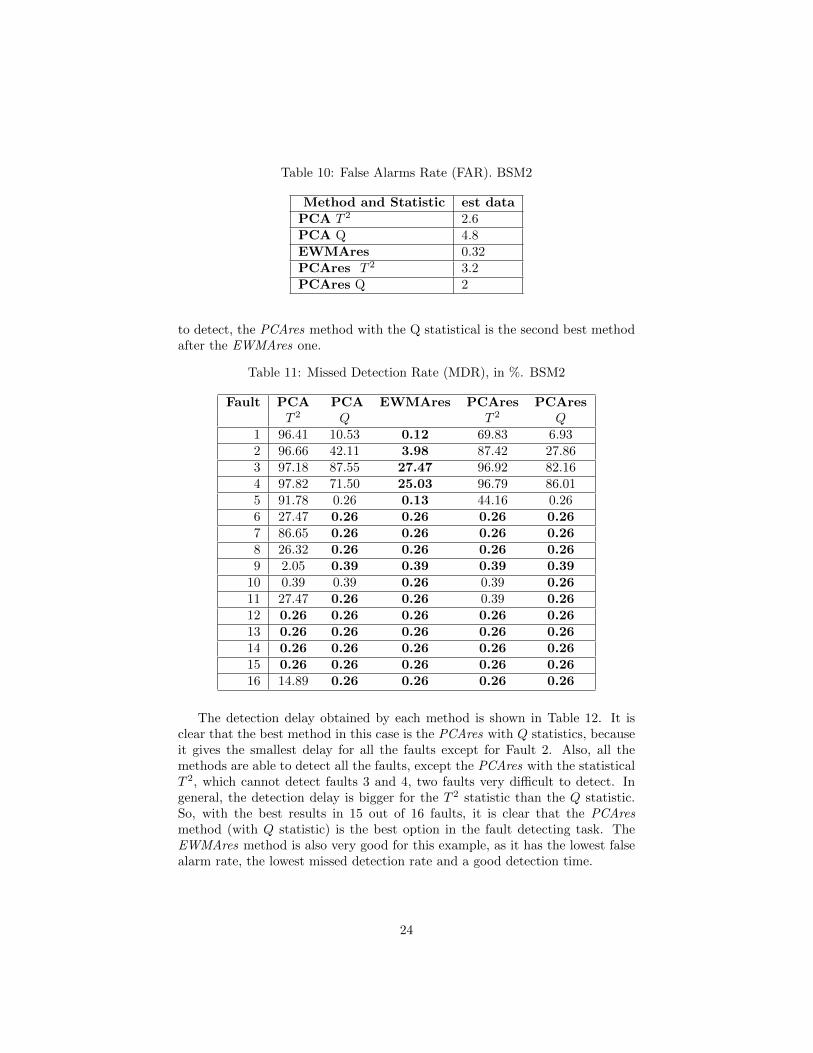
Table 10: False Alarms Rate (FAR). BSM2

Method and Statistic est dataPCA T 2 2.6PCA Q 4.8EWMAres 0.32PCAres T 2 3.2PCAres Q 2

to detect, the PCAres method with the Q statistical is the second best methodafter the EWMAres one.

Table 11: Missed Detection Rate (MDR), in %. BSM2

Fault PCA PCA EWMAres PCAres PCAresT 2 Q T 2 Q

1 96.41 10.53 0.12 69.83 6.932 96.66 42.11 3.98 87.42 27.863 97.18 87.55 27.47 96.92 82.164 97.82 71.50 25.03 96.79 86.015 91.78 0.26 0.13 44.16 0.266 27.47 0.26 0.26 0.26 0.267 86.65 0.26 0.26 0.26 0.268 26.32 0.26 0.26 0.26 0.269 2.05 0.39 0.39 0.39 0.39

10 0.39 0.39 0.26 0.39 0.2611 27.47 0.26 0.26 0.39 0.2612 0.26 0.26 0.26 0.26 0.2613 0.26 0.26 0.26 0.26 0.2614 0.26 0.26 0.26 0.26 0.2615 0.26 0.26 0.26 0.26 0.2616 14.89 0.26 0.26 0.26 0.26

The detection delay obtained by each method is shown in Table 12. It isclear that the best method in this case is the PCAres with Q statistics, becauseit gives the smallest delay for all the faults except for Fault 2. Also, all themethods are able to detect all the faults, except the PCAres with the statisticalT 2, which cannot detect faults 3 and 4, two faults very difficult to detect. Ingeneral, the detection delay is bigger for the T 2 statistic than the Q statistic.So, with the best results in 15 out of 16 faults, it is clear that the PCAresmethod (with Q statistic) is the best option in the fault detecting task. TheEWMAres method is also very good for this example, as it has the lowest falsealarm rate, the lowest missed detection rate and a good detection time.

24

Table 12: Detection delays (in samples). BSM2

Fault PCA PCA EWMAres PCAres PCAresT 2 Q T 2 Q

1 258 772 23 253 122 258 725 184 253 1933 258 211 223 nd 1944 259 278 223 nd 2085 259 7 3 2 26 726 7 3 2 27 541 7 3 2 28 775 7 3 2 29 506 8 4 3 3

10 8 8 3 3 211 775 7 3 3 212 7 7 3 2 213 7 7 3 2 214 7 7 3 2 215 7 7 3 2 216 692 7 3 2 2

nd=not detected

5. CONCLUSIONS

This paper presents a dynamic and non-linear fault detection and diagnosismethodology. The proposed methodology explicitly accounts for the dynamicrelations in the process data through dynamic feature selection, and for thenon-linear relationship between the variables of the process through a time-series model available to capture both the non-linear, if it exists, and the dy-namic correlation in the process data. After that the residuals, which are thedifference between the process measurements and the output of the model, aremonitored using conventional SPC charts, such as the EWMA control chart ifthe residuals are evaluated individually, or a Multivariate Statistical ProcessControl (MSPC) chart when the residuals are processed all together; in thiscase they are evaluated with the PCA algorithm and the classical Hotelling’sand SPE statistics.

This methodology was applied to two plants: the Tennessee Eastman Processand a Waste Water Treatment Plant, and compared with other fault detectionmethods. The method based on individual residuals with the univariate con-trol chart (EWMA) gives a good performance, but it is not better than theother methods of the comparison, specially for the TE plant, but it does givea very good result with the WWTP. However, the method based on the PCAof residuals is the best in the comparative, giving the highest number of faultsdetected and the lowest detection time (delay). The fault alarms rate (FAR) isalso better than the other existing methods for the test data, while the missed

25

detection rate (MDR) outperforms the other methods and is equivalent to thebest one (CVA with the Tr statistic). So, comparisons with the four indexes(number of faults detected, FRA, MDR and detection delay) obviously demon-strate the effectiveness and superiority of the proposed methodology, speciallyfor the PCAres with the Q statistic. Finally, these examples demonstrate thatthe proposed methodology efficiently detects faults for non-linear and dynamicprocesses.

Acknowledgment

This work has been partially supported by the Spanish Ministry of Econ-omy, Industry and Competitiveness and the European Regional DevelopmentFund (FEDER) through the Projects: DPI2015-67341-C2-2-R, TIN2013-47210-P, TIN2016-81113-R and to the Junta de Andalucıa through the project: P12-TIC-2958

6. References

[1] Z. Ge, Z. Song, F. Gao, Review of recent research on data-based processmonitoring, Industrial & Engineering Chemistry Research 52 (2013) 3543–3562.

[2] V. Venkatasubramanian, R. Rengaswamy, S. Kavuri, A review of processfault detection and diagnosis. Part I: Quantitative model-based methods,Computers & Chemical Engineering 27 (2003) 291–311.

[3] V. Venkatasubramanian, R. Rengaswamy, S. Kavuri, A review of processfault detection and diagnosis. Part II: Qualitative models and search strate-gies, Computers & Chemical Engineering 27 (2003) 313–326.

[4] V. Venkatasubramanian, R. Rengaswamy, S. Kavuri, K. Yin, A reviewof process fault detection and diagnosis. Part III: Process history basedmethods, Computers & Chemical Engineering 27 (2003) 327–346.

[5] A. Bakdi, A. Kouadri, A new adaptive PCA based thresholding scheme forfault detection in complex systems, Chemometrics and Intelligent Labora-tory Systems 162 (Supplement C) (2017) 83 – 93.

[6] S. Qin, Survey on data-driven industrial process monitoring and diagnosis,Annual Reviews in Control 36 (2012) 220–234.

[7] W. Ku, R. Storer, C. Georgakis, Disturbance detection and isolation bydynamic principal component analysis, Chemometrics and Intelligent Lab-oratory Systems 30 (1995) 179–196.

[8] T. Villegas, M. J. Fuente, G. I. Sainz-Palmero, Fault diagnosis in a wastew-ater treatment plant using dynamic independent component analysis, in:18th Mediterranean Conference on Control & Automation (MED), IEEE,2010, pp. 874–879.

26

[9] J. Huang, X. Yan, Dynamic process fault detection and diagnosis based ondynamic principal component analysis, dynamic independent componentanalysis and bayesian inference, Chemometrics and Intelligent LaboratorySystems 148 (2015) 115–127.

[10] A. Simoglou, E. Martin, A. Morris, Statisical performance monitoring ofdynamic multivariate processes using state space modeling, Computers &Chemical Engineering, 26(6) (2002) 909–920.

[11] H. Kaneko, K. Funatsu, A new process variable and dynamics selectionmethod based on a genetic algorithm-based wavelength selection method,AIChE Journal 58(6) (2012) 1829–1840.

[12] M. Kramer, Autoassociative neural networks, Computers & Chemical En-gineering 16 (1992) 313–328.

[13] W. Yan, P. Guo, L. Gong, Z. Li, Nonlinear and robust statistical processmonitoring based on variant autoencoders, Chemometrics and IntelligentLaboratory Systems 158 (2016) 31–40.

[14] B. Schokopf, A. Smola, K. R. Muller, Nonlinear component analysis as akernel eigenvalue problem, Neural Computation 10 (1998) 1299–1319.

[15] J. Lee, C. Yoo, S. W. Choi, P. A. Vanrolleghemb, I. Lee, Nonlinear processmonitoring using kernel principal component analysis, Chemical Engineer-ing Science 59 (2004) 223–234.

[16] J. Hunter, The exponentially weighted moving average, Journal of QualityTechnology 18(4) (1986) 203–210.

[17] D. Garcia-Alvarez, M. J. Fuente, G. I. Sainz-Palmero, Design of residuals ina model-based fault detection and isolation system using statistical processcontrol techniques, in: ETFA2011, 2011, pp. 1–7.

[18] G. James, D. Witten, T. Hastie, R. Tibshirani, An Introduction to Statis-tical Learning, Springer New York, 2013.

[19] S. Wold, M. Sjostrom, L. Eriksson, PLS-regression: a basic tool of chemo-metrics, Chemometrics and Intelligent Laboratory Systems 58 (2001) 109–130.

[20] R. H. Shumway, D. S. Stoffer, Time Series Analysis and its Applications,Springer-Verlag Berlin, 2006.

[21] J. D. Gooijer, R. J. Hyndman, 25 years of time series forecasting, Interna-tional Journal of Forecasting 22 (2006) 443–473.

[22] G. Box, G. Jenkins, Time Series Analysis: Forecasting and Control, Holden-Day San Francisco, 1976.

27

[23] M. Kuhn, K. Johnson, Applied Predictive Modeling, Springer-Verlag NewYork, 2013.

[24] K. Hornik, M. Stinchcombe, H. White, Multilayer feedforward networksare universal approximators, Neural Networks 2(5) (1989) 359–366.

[25] G. I. Sainz-Palmero, M. J. Fuente, P. Vega, Recurrent neuro-fuzzy mod-elling of a wastewater treatment plant, European Journal of Control 10(2004) 83–95.

[26] M. Khashei, M. Bijari, An artificial neural network (p, d,q) model fortimeseries forecasting, Expert Systems with Applications 37 (2010) 479–489.

[27] E. Heidari, M. A. Sobati, S. Movahedirad, Accurate prediction of nanofluidviscosity using a multilayer perceptron artificial neural network (MLP-ANN), Chemometrics and Intelligent Laboratory Systems 55 (2016) 73–85.

[28] V. Vapnik, The Nature of Statistical Learning Theory, Springer New york,1995.

[29] K. W. Lau, Q. H. Wu, Local prediction of non-linear time series usingsupport vector regression, Pattern Recognition 41 (2008) 1539–1547.

[30] E. E. Elattar, J. Goulermas, Q. Wu, Electric load forecasting based onlocally weighted support vector regression, IEEE Transactions on Systems,Man and Cybernetics. 40(4) (2010) 438–447.

[31] S. Saludes-Rodil, M. J. Fuente, Fault tolerance in the framework of supportvector machines based model predictive control, Engineering Applicationsof Artificial Intelligence 23 (2010) 1127–1139.

[32] A. Ferrer, Statistical control of measures and processes, ComprehensiveChemometrics - Chemical and Biochemical Data Analysis 1 (2009) 97–126.

[33] D. Garcia-Alvarez, G. I. Sainz-Palmero, M. J. Fuente, P. Vega, Fault detec-tion and diagnosis using multivariate statistical techniques in a wastewatertreatment plant, in: IFAC Proceedings Volumes, Vol. 42, 2009, pp. 952–957, 7th IFAC Symposium on Advanced Control of Chemical Processes.

[34] W. Shewhart, Application of statistical methods to manufacturing prob-lems, Journal of the Franklin Institute 226 (2) (1938) 163 – 186.

[35] R. Woodward, P. Goldsmith, Cumulative sum techniques, Mathematicaland Statistical Techniques for Industry, Oliver & Boyd Edinburgh, 1964.

[36] E. S. Page, Continuous inspection schemes, Biometrika 41 (1-2) (1954)100–115.

[37] I. Jolliffe, Principal Component Analysis, Springer Verlag New York, 2002.

28

[38] T. Kourti, J. MacGregor, Multivariate SPC methods for process and prod-uct monitoring, Journal of Quality Technology 28 (1996) 409–428.

[39] C. F. Alcala, S. J. Qin, Reconstruction-based contribution for process mon-itoring, Automatica 45 (2009) 1593–1600.

[40] J. E. Jackson, A User’s Guide to Principal Components, Wiley New York,1991.

[41] M. Frigge, D. C. Hoaglin, B. Iglewicz, Some Implementations of the Box-plot, The American Statistician 43(1) (1989) 50–54.

[42] E. L. Russell, L. H. Chiang, R. D. Braatz, Fault detection in industrialprocesses using canonical variate analysis and dynamic principal componentanalysis, Chemometrics and Intelligent Laboratory Systems 51(1) (2000)81–93.

[43] K. Detroja, R. Gudi, S. Patwardhan, Plant-wide detection and diagno-sis using correspondence analysis, Control Engineering Practice 15 (2007)1468–1483.

[44] C. Tong, T. Lan, X. Shi, Fault detection and diagnosis of dynamic processesusing weighted dynamic decentralized PCA approach, Chemometrics andIntelligent Laboratory Systems 161 (Supplement C) (2017) 34–42.

[45] J. J. Downs, E. F. Vogel, A plant-wide industrial process control problem,Computers & Chemical Engineering 17 (1993) 245–255.

[46] L. Chiang, E. Russell, R. Braatz, Fault Detection and Diagnosis in Indus-trial Systems, Springer-Verlag London, 2000.

[47] B. Jiang, D. Huang, X. Zhu, F. Yang, R. D. Braatz, Canonical vari-ate analysis-based contributions for fault identification, Journal of ProcessControl 26 (2015) 17–25.

[48] Y. Zhang, Fault detection and diagnosis of nonlinear processes using im-proved kernel independent component analysis (KICA) and support vec-tor machine (SVM), Industrial & Engineering Chemistry Research 47 (18)(2008) 6961–6971.

[49] J. Alex, L. Benedetti, J. Copp, K. Gernaey, U. Jeppsson, I. Nopens,M. Pons, C. Rosen, J. Steyer, P. Vanrolleghem, Benchmark SimulationModel no. 2 (BSM2), Tech. rep., IWA Taskgroup on Benchmarking of Con-trol Systems for WWTPs. Department of Industrial Electrical Engineeringand Automation, Lund University, Lund, Sweden, (2008).

[50] I. Nopens, L. Benedetti, U. Jeppsson, M.-N. Pons, J. Alex, J. B. Copp,K. V. Gernaey, C. Rosen, J.-P. Steyer, P. A. Vanrolleghem, Benchmarksimulation model no 2: finalisation of plant layout and default controlstrategy, Water Science & Technology 62 (2010) 1967–1974.

29