
fatigue damage modeling in solder interconnects using a cohesive zone approach
Upload
nguyentuyenCategory
view
214download
0
FATIGUE OF SOLAR CELL INTERCONNECTS
G.R. Mon
Jet Propulsion. Laborat;ory California Institute of Technology
Pasadena, California 91109
Interconnects, metallic ribbons connecting and providing electrical continuity between photovoltaic cells, have been observed to fracture in terrestrial applications environments- (Figures. 1 and 2). The degradation mechanism has been ident~fied as mechanical fatigue resulting from diurnal thermal variations that can impose large cyclical strains upon poorly designed module/interconnec~ systems (Figure 3). Good design techniques-for example, providing adequate stress relief ~oops and matching substratecell-interconnect thermal expansion coefficients, etc.--will minimize interconnect fractures, b~t o~ly a systematic design algorithm using life-cycle energy costing to effect the many cost-performance trade-offs will result in optimal (long life, minimum cost) performance. Such an . algorithm has been deve'loped by the Engineering Sciences Area of the Flat-Plate Solar Array Project at the Jet .Propulsion Laboratory (Figure 4).
The optimization algorithm fe.atures three computational procedures, each of which is discussed brie~~Y. The first procedure (Figure 5), called "Interconnect Failure Prediction Algorithm," calculates the strain in interconnects from module geometry and materials data (Figure 6) and site temperature histories (Figures 7 through .. 9). Strain computations (Figure 10) are facilitated by the use of-nomographs that incorporate the results of computer-generated finite element solutions (Figure 11). The computed strains are used in conjunction with interconnect material statistical fatigue curves to estimate the e~pected fraction of failed interconnects at the end of the operational life of the array field.
The material statistical fatigue curves are obtained experimentally. Candidate interconnect materials (Figure 12) were tested in several geometries (Figure 13) on an apparatus (Figure 14) designed to ~imu1ate mechanically the cyclical strain cycles induced by diurnal thermal cycles in the field. Raw data are gathered in the form of curves of fracture probability versus cycles to failure at the constant test strain (Figure 15). A global least-squares minimization routine is. used to fit a suitable function to these data; the resulting set of curves are the material fatigue (strain-cycle) curves parameterized by failure probability (Figures 16 through 20). A comparison of test results (Figure 21) reveals the fatigue-performance superiority of the clad materials.
The material statistical fatigue curves find use in module design and in interconnect-failure prediction (Figure 22) and in thermal-cycle qualification test design (Figures 23 through 25). In a thermal cycling test, both the strain (temperature) and the cycle rate are accelerated. The material fatigue curves are used to determine the number of test cycles and allowable interconnect-failure rates to guarant~e a maximum allowable field failure rate (Figure 25). Results of thermal cycle ~testing are presented (Figure 26).
337
In: Proceedings of the Flat-Plate Solar Array Project Research Forum on Quantifying Degradation(December 6-8, 1982, Williamsburg, Virginia), JPL Publication 83-52, JPL Document 5101-231,DOE/JPL-1012-89, Jet Propulsion Laboratory, Pasadena, California, June 1, 1983, pp. 337-378.

Correlation of field failure data and thermal cycling test data with the experimental fatigue data is good (Figure 27).
The second computational procedure associated with the optimization algorithm is the Array Degradation Analysis (Figure 28), which determines the loss of array power, and hence the energy output reduction, resulting from specified levels of interconnect redundancy and failure probability. The power reduction at 20 years (Figure 29) follows from the array circuit configuration (Figure 30) and the appropriate array power loss data (Figure 31).
The final computational procedure compr1s1ng the optimization algorithm is the Life-Cycle Energy Cost Analysis (Figure 32). The important parameters influencing the analysis include the (fatigue-related) relative array energy output, interconnect resistivity and shadowing losses, and materials and fabrication costs (Figures 32 and 33). The relative energy output is determined as the area under the array power output curves (Figures 34 and 35). This, together with plant efficiency considerations (Figure 36), interconnect material and fabrication costs (Figures 37 through 41), and other parameter values (Figure 42), when substituted into the life-cycle energy costing equation (Figure 32), yield the solution cost curves for each candidate material (Figures 43 through 47).
The material cost curves have common features. The dotted curves give cost increments due to fatigue-free interconnects. The left ends of these curves reflect I2R-losses; the right ends, the materials costs. The solid lines indicate cost increments due to fatigue failures. In all cases there exists a critical strain level (thickness) beyond which costs increase rapidly. The curves suggest designing at about half the critical thickness. The curves also suggest using double interconnect redundancy; more redundancy results in higher cost, while use of a single interconnect gives inadequate protection against random (non-fatigue-related) failures, assumed to be 5 per 1000 in 20 years.
The cost solutions for doubly redundant interconnect systems (Figure 48) reveal that OFHC copper and the 33 Cu/33 INV/33 eu are cost effective, the latter perhaps more so because it provides for a greater thickness design margin.
A final note: the analysis reveals that the increment in life-cycle energy costs due to interconnects may be as much as 15% of the total life-cycle energy cost of the array.
338

Figure 1. Broken PV Cell Interconnect
339

Figure 2. Cell Interconnect Configurations (Block II Module, Manufacturing Variations)
......... - -.0 h 7/_' - --...l
HIGHEST STRESSED
I I ~-~fo72 --~
LOWEST STRESSED
340

Figure 3. Interconnect Fatig~,~ F.ailure Mechanism
DAY -TO-N IGHT DIFFERENT THERMAL
TEMPERATURE CYCLING EXPANSION COEFFICIENTS
OF MODULE OF SOLAR CELLS AND THEIR SUBSTRATES
l( RELATIVE MOTION BETWEEN} ADJACENT SOLAR CELLS
CYCLIC STRAINING OF CELL INTERCONNECTS
Figure 4. Cost-Optimal Reliability Design Algorithm
ALTER END-OF-LIFE POWER
REDUCTION AND/OR ARRAY CONFIGURATION
MAXIMUM ALLOWABLE
INTERCONNECT STRAIN
N N
341

Figure 5. Interconnect Failure Prediction Algorithm
FINITE ElEMENT COMPUTER CODE DR RELATED IOMOGRAPHS ANO CHARTS
~NTERCONNECT
MATERIAL . STATlimCAL j
L FATIGUE CURVESJ
Figure 6. Effective Interconnect Displacement Due to Differential Thermal Expansion
_ D a CELL DIAMETER-I
- C - CELL CENTER DISTANCE - --. r- ~~~~~~~~~~
1 I 1... ____ _
as
-g-
AT TEMPERATURE T AT TEMPERATURE T + AT
ENCAPSULANT
'--4 SUBSTRATE ,
SUBSTRATE EXPANSION
{) - (asC - acO - algI AT - [(as - acl C + (ac - all gJ AT
342

U a
.-: z u.J
as :E c:z: u.J :> 0 <Xl <[
u.J a: :::>
""" c:z: a: u.J Q..
:E u.J
""" ~ z ;::: <[ a: u.J Q.. 0 u.J -' :::> 0 0 :E
Q.. 0
""" <l
Figure 7. 1979 Temperatures at New River, Arizona
35
30
25
20
15
10
5
0
TEMPERATURE, ac
MONTH AVG. HIGH AVG. LOW dTD
JANUARY 11.7 2.B B.9 FEBRUARY lB.3 5.0 133 MARCH 20.6 7.B 12.B APRIL 27.2 10.6 16.7 MAY 31.1 16.7 14.4 JUNE 3B.9 22.B 16 1 JULY 41.1 25.0 16.1 AUGUST 3B.9 23.3 15.6 SEPTEMBER 3B.9 24.4 14.4 OCTOBER 30.6 16.1 14.4 NOVEMBER 20.0 7.2 12.B DECEMBER 19.4 6.7 12.B
AVERAGE dTo = 14.0 ac
Figure 8. Module Operating Temperature (Block II Fiberglass Substrate Module)
SOLAR INSOLATION, mW/cm2
343

Figure 9. Cell Interconnect Deflection
o Total Temperature Excursion
~TDN = 14°C (Yearly Average)
~TOp = 32°C (At 100 mW/cm2)
~ T = 46°C (Yearly Average)
o Thermal Expansion Coefficients
as = 2.78 X 10⁻⁵/°C (Fiberglass Substrate)
ac = .29 X 10-5/°C (Silicon Solar Cell)
o Cell Interconnect Deflection
o = (asC - acD) ~ T
= .0035 in.
Figure 10. Deformed Shape and Strain for Typical Field-Stressed Interconnect
012
..§ 008
== Z <i: 004 a:: I-en
0
--
/ /
./ _/
_ - _ ~ UNDEFDRMED SHAPE /' ..... --<:
/1 "DEFORMED SHAPE
, , ' ..... --
\1-01 .&-------- 072 In -------tCllo>-l~ I
~ l) Q 0035 In
344
•

Figure 11. SC-Interconnect Nomograph
Note 9 IS the HOrizontal Distance Between Interconnect A ttachment POints
Figure 12. Candidate Interconnect Materials
• Homogeneous Materials
• 1100 aluminum • OFHC 1/4·hard copper
• Clad Materials
• 33.3 Cu/33.3 INV/33.3 Cu • 12.5 Cu/75.0 INV/12.5 Cu • 16 Cu/6a SS/16 Cu
345

I 071
Figure 1 3. Geometry of Interconnects
C46
\c--CEL- L --'I~J ~ CELL?
0 .95 r--1.91 - -1
0 .95
0 .25 ~
'S-C:-:CEL-L ----1( --.L f I CELL ? I l - 095 Ir-19 '~
SC
I ~0. 25 '---+---"91-1 T
All DIMENSIONS ARE IN MILLIMETE RS
, S CELL ~05B I ol8
~- j ,\ I j ~I I ~ELl? 0 .25
, i -"148
-! I 0 9 5
-- 14 2
1 91 - -
aT sx
Figure 14. Interconnect Strain-Cycle Apparatus
346

IL.I
<I ,
z C::( a:: .-en
Figure 15. Experimental Data: OFHC Copper Interconnects
100
10-2
r" I "''''r ... ""'I 1 i~ "TTTf" "T rT"T"""r • I nrrHI r '·'"Ql I .-M",8 ~ ~~~-Man-:tO'J~ I ... -eDOM M .... N..-Nomoc.o o ~ ONMO 0 000- 0 ..... 00
I ~ -0000 0 oo~O~~~o..,,,, 0001111 111111 0 ~""
_ 0 II II II \4.1....., ,.... ... ,.... II II II II II II 08:
a. " ""''''..,,, "..,.., ... ",~~,,"'';0o ~ "',,<l<l .... x .... ux..,<l".., 0 t::: .., NI- NO VJ 0 cncn~NXUX~ II II :. ,NOOOOO 0000 rnc.nCl) ~\U CD SX. _ 0 M M M M M M M M M goo 0 g <l <l
~ 1 0 s~ '~7 t ~,1 f' \j ~) J ~~/ M J) ~ ~ if Dr '.';! i" 11; II!) I /} ~ 7 7 ~ 0 8 z' - ': I ' U 1/ r f I ~ 1/ J
~ 06:: ! /1/ If r 1/ i / ) I!/!r J u ,I I I II 0 ( J.... .... '
I 04 i . i /))/1: i ) If I I;l g!.1 r' ~ ~ ~ l !! i ) ji r ); ~ 1 ~02-j! I ~I ~
{,I l;J. / I I M
. j ··r/. ..- I o __ .~ . ..:.-" ,~wol ••• "",! I' 'ill.UL ' ... 10 1 O' 1 0 3 10' 10' 10'
CYCLES N
Figure 16. Statistical Fatigue Curves for Tinned, Annealed 1100 Aluminum
p= 0.99 0.80 0.50 0.30 0.10 0.03
log~€ = - 0.3911 log N - 0.8930 + 0.6581 p -n.7058p2 + 0.2974p3
10-3~~~~~~~~-w~~~~~~~~ 101 102 103 104 105 106
CYCLES, N
347

"'"' <J ,
:2 C( a: .-CIJ
10- 1
10- 2
Figure 1 7. Statistical Fatigue Curves for OFHC ~ -Hard Copper .
log LlE = - 0.3228 log N - 1.0148 + 0.9998p -1.4839p2 + 0.9019p3
10-3~~~~~~~~~~~~~~~~~~~ 101 102 103 104 105 106
CYCLES, N
348

\U
Figure 18. Statistical Fatigue Curves for 33 Cu / 33 Inv / 33 Cu
(ANNEALED AND 20% COLD·ROLLED) P= 0.99 0.80
10- 1 0.50
<J 0.30 ~
2 « a:: ..en
10- 2
log ~E = - 0.3821 log N - 0.4771 + 0.6238p -0.9644p2 + 0.6535p3
10-3~~~~~~~~~~~~~~~~~~ 10 1 102 103 104 105 106
CYCLES, N
349

/
Figure 19. St~tistical Fatigue Curves for Cladding, 12.5 Cu / 75 Inv / 12.5 Cu
p= 0.99
, 0.80 10-1~~
ILl ~~~ <1
0.50 0.30 0.10 0.03
2: c::r:: a:: ~ en
10- 2
log AE :: - 0.2719 log N - 0.6995 + 0.4638p -0.7090p2 + 0.4171 p3
CYCLES, N
350

IoU
<J :z « ex:: ~ en
Figure 20. Statistical Fatigue Curves for Cladding (16 Cu / 68 55 / 16 Cu)
p= 0.99 0.80 0.50 0.30
. 10- 2
log ~E = - 0.3871 log N - 0.4723 + 0.3829p -0.3837p2 + 0.2234p3
10-3~~~~~~~~~~~~~~~~~~ 101 102 103 104 105 106
CYCLES,· N
Figure 21. Experiment Fatigue Test Results
.·Comparison at same strain level for which 10% of copper interconnects fail in 20 years
Material
Aluminum Copper 33 Cu/33 INV/33 Cu 12.5 Cu/75.0 INV/12.5 Cu 16 Cu/68 SS/16 Cu
351
Years to 10% failures
7 20
106 1030
85

Figure 22. Statistical Fatigue Curves for OFHC ~ ~Hard Copper
PREDICTION AND DESIGN USING FATIGUE CURVES --- .,.~ ... ~ .~ ~'~"""'~~-" "l
CYCLES N
Figure 23. Typical Thermal-Cycle Test Profile and Test Acceleration Factor
I" MAXIMUM CYCLE TIME ---~
~ +90 ...; a: . ::;) to-
"" a: .... D.. :::e .... to--' ~ -40 ~
Test Profile
2
• Amplitude: 6TTEST = 130°C • Duration: N = 200 cycles
Test Purpose
3
• To qualify modules for typical field application (6 TFIElD = 46°C)
4 5
CONTINUE FOR N CYCLES
I' • I I \ I
, I I ! \ I I _____ J
I
6
TIME, h
352
Test Acceleration Factor • Since interconnect strain varies
linearly with temperature change.
6ETEST = 6 TTEST = 130 = 2.83 6EFIELD 6 TFIELD 46

Figure 24. Statistical Fatigue Curves for OFHC ~ -Hard Copper Thermal-Cycle Test Design
THERMAL CYCLE TEST' DESIGN
10-2 .1tFIElD
10-3~~~~~~~~~~~~~~~~~~~
101 102 103 104 105 106
CYCLES, N
Figure 25. Thermal-Cycle Qualification Test Design
10000~--------~--------~~~------~---------'
rr~f-20
';Ie
~ w > ~ 10.00 w Ill: 3 ~ Ien w l-
I~ w
~ 1.00 ~ Ill: w I-~
3.5%
/-+-#--15 ~f---l0
#---5 #----3
CONDITIONS
INTERCONNECT FIELD FAILURE LEVEL, %
o DFHC COPPER INTERCONNECTS • FIELD SITE: ~T - 4SoC
• TEST AMPLITUDE: ~ T - 130 0 C
• QUALIFICATION FOR 20·yr APPLICATION
010~ ______ ~~~~ ____ ~~ ______ ~~~ __ ~~~ 10 1 DO 1000 10,000 100,000
TEST CYCLES N
353
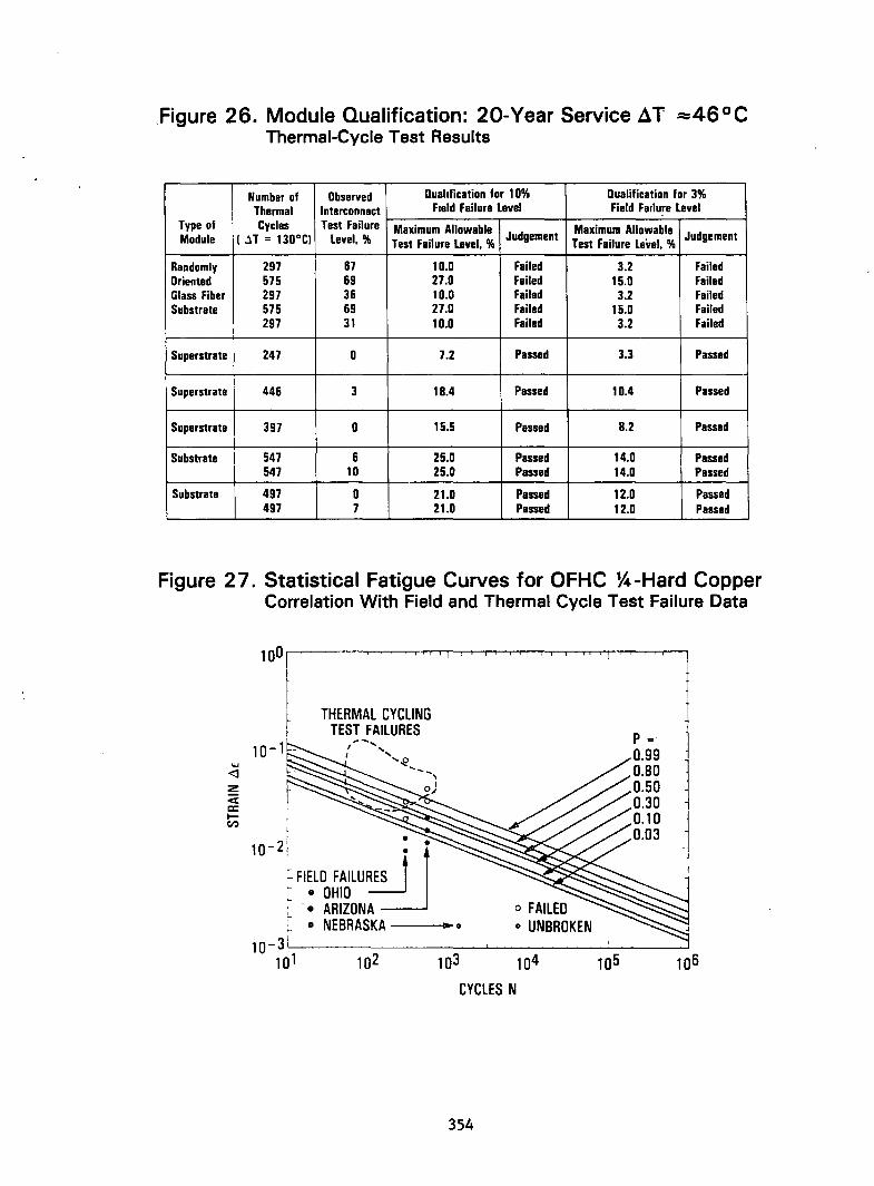
,Figure 26. Module Qualification: 20-Year Service ~T ~46°C Thermal-Cycle Test Results
Number of Observed Quahfication for 1 0% Qualification for 3% Thermal Interconnect Field Failure Level Field Failure Level
Type of Cycles Test Failure Maximum Allowable Maximum Allowable Module ( .H = 130a C) Level. % Test Failure Level. %
Judgement Test Failure Level. %
Judgement
Randomly 297 67 10.0 Failed 3.2 Failed Oriented 575 69 27.0 Failed 15.0 Failed Glass Fiber 297 36 10.0 Failed 3.2 Failed Substrate 575 69 27.0 Failed 15.0 Failed
I 297 31 10.0 Failed 3.2 Failed
Superstrate I 247 0 7.2 Passed 3.3 Passed i
S ! uperstrate ' 446 3 lB.4 Passed 10.4 Passed
Superstrate 397 0 15.5 Passed B.2 Passed
Substrate 547 6 25.0 Passed 14.0 Passed 547 10 25.0 Passed 14.0 Passed
Substrate
I 497 0 21.0 Passed 12.0 Passed 497 7 21.0 Passed 12.0 Passed
Figure 27. Statistical Fatigue Curves for OFHC % -Hard Copper Correlation With Field and Thermal Cycle Test Failure Data
,
i 'i i I
THERMAL CYCLING TEST FAILURES -- .... I ....
I ' .... ~ .... -.... ,
0)
10-2~ FIELD FAILURES j 1 - • OHIO ;- '. ARIZONA .' • NEBRASKA .. 0
10- 3 !,-, ----
101 102 103
CYCLES N
354
i I i " i I , i

Figure 28. Array Degradation Analysis Algorithm
INTERCONNECT REDUNDANCY
-----r
ARRAY CIRCUIT f-CONFIG- REQUIRED REQUIRED REQUIRED URATION SUBSTRING CELL INTERCONNECT
( t'\ FAILURE f- FAILURE 1"1--. FAILURE '1/ \L/ PROBABILITY PROBABILITY PROBABILITY
ARRAY POWER FSS Pc p
REDUCTION AT ARRAY r--
DESIGN LIFE fy
Figure 29. Array Power Reduction at 20 Years
20-YEAR INTERCONNECT ARRAY POWER REOUCTION AT 20 YEARS
FAILURE ty PROBABILITY
PI r = 1 2 3 4 5 6
0.005 0.125 0.0018 0 0 0 0 0.010 0.240 0.0059 0 0 0 0 0.050 0.71 0.05 0.0070 0.0004 0 0 0.100 0.96 0.24 0.029 0.0055 0.0007 0 0.150 1.00 0.31 0.054 0.019 0.005 0.0013 0.200 1.00 0.57 0.19 0.038 0.013 0.003 0.300 1.00 0.90 0.46 0.20 0.048 0.023 0.400 1.00 1.00 0.90 0.45 0.26 0.085 0.500 1.00 1.00 1.00 0.80 0.53 0.32
355

z 0 -u <t: 0::: ~
VI VI 0 -' 0::: ... :s: 0 CL.
>-<t: 0::: 0::: <t:
Figure 30. Example Design Parameters
Array.Configuration:
• 8 parallel by 11 series cells per series block
o 57 series blocks per branch circuit
• One series block per diode
• VARRAY = 250 volts
Figure 31 . Array Power Loss
1.0 ~ t 8 PARALLEL STRINGS
FF = O. 70 ~ r
! 0.1 ----
r
~ O.Ol'b
~ ~
0.001
1 SERIES BLOCK PER DIODE
SERIES BLOCKS PER BRANCH CIRCUIT
Ql LO
FSS' SUBSTRING FAILURE DENSITY
356

,
Figure 32. Effect of Mat~rial Properties on Life-Cycle Energy Costs
BALANCE OF PLANT COSTS ,
INITIAL PLANT COST
COST OF INTERCONNECtS LlFE.CYCLE
LlFE·CYCLE ENERGY COST
""-""-
" \
" " CB +
R =
/ ANNUAL
10 /
/
SOLAR INSOLATION
\ / / OPERATION AND
_ MAINTENANCE I _
CI + CM - COSTS
1]---- PLANT EFF~CIENCY (RESISTIVITY AND SHADOWING) €LC
"-
" " RELATIVE ENERGY OUTPUT (FATIGUE)
Figure 33. Module Interconnect Assessment Algorithm
REPRESENT A TlVE ARRAY CIRCUIT ~ CONFIGURATION
ELECTRICAL ARRAY ENERGY
~ EFFICIENCY ~ OUTPUT DETERMINATION DETERMINATION
REPRESENT A TlVE INTERCONNECT MODULE INTER· r-- FAILURE RATE ~ CONNECT DESIGN DETERMINATION
+ LlFE·CYCLE
INTERCONNECT LlFE·CYCLE ECONOMIC
~ ADD·ON COST ~ ENERGY
~ MERIT OF
COST INTERCONNECT DETERMINATION
ANALYSIS MATERIAL
357

Figure 34. Array Power Output Fraction vs Years of Operation
Figure 35. Life-Cycle Energy Fractions
20·Year Cumulative Interconnect Life·Cycle Energy Fraction € lC Failure Probability
PI r = 1 2 3 4 5 6
0.005 17.8 19.95 20 20 20 20 0.010 16.6 19.90 19.96 20 20 20 0.050 11.7 19.45 19.89 19.98 20 20 0.100 7.7 18.2 19.76 19.92 19.98 20 0.150 4.4 16.5 19.55 19.88 19.96 20
.. 0.200 2.25 13.2 18.47 19.55 19.88 20 0.300 1.74 11.2 17.1 18.65 19.66 19.91 0.400 1.60 9.9 15.17 17.1 18.7 19.15 0.500 1.5 8.9 13.2 15.6 17.4 17.9
358

Figure 36. Total Plant Efficiency 7J
Equations:
( LW \r, 120)
71 = 710 1 - -A-7~ - PO
o =.!e.. wt
P = Px ----
2x + y(:~)
Symbols: . p = electrical resistivity of cladding
xlylx = thickness ratio of claddings Px,y = electrical resistivity of materi~ls x,y f,w,t = length, width, and thickness of interl!onnect
o = resistance of interconnect I = solar cell current at maximum power
Po = cell power output L: = ratio of cell area covered by interconnect to total cell area
710 = baseline plant efficiency
359

. Figure 37. Add-On Cost for Interconn-ects vs Thickness With Interconnect Redundancy as Parameter' (Tinned, Annealed 1100 Aluminum)
N 7 E
0(1)-
6 ~ 6 u 5
UJ 4 ~ u 5 LU 3 z z-0 4 u ~ LU ~ z 3 ~ r=l 0 u.. ~ UJ
2 0 U
z 1 0 . CJ CJ <C
0 1 2 3 4 5 6 7 8 THICKNESS t, mils
360
9
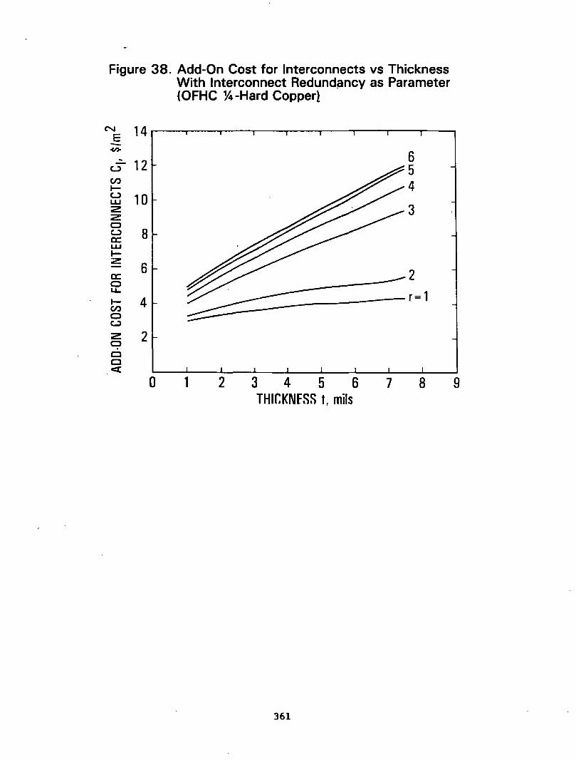
Figure 38. Add-On Cost for Interconnects vs Thickness With Interconnect Redund~ncy as Parameter (OFHC %-Hard Copperl
N 14 E -<I>
- 12 u CIJ t-U 10 LU 2: 2: 0 u 8 a:: LU t-2:
6 a:: 0 LL
t- 4 CIJ 0 U
2: 2 C? c c «
0 1 2
6 5 4
3
2 ~----==r=1
3 4 5 6 7 8 THIr.KNfSS t, mils
361
9

Figure 39. Add-On Cost for Interconnects vs Thickness " With Interconnect Redundancy as Parameter (33 Cu / 33 Inv / 33 Cu)
N E
<1)0
,
u CJ:) .-u w Z Z 0 u a: w .-z a: 0 u.. .-CJ:)
0 u z 0 . 0 0 oCt
17
15
13
11
9
7
5
30 1 2 3 '4 5
6 5 4
3
~_-- r=1
B 9 THICKNESS t, mils
362

Figure 40. Add-On Cost for Interconnects vs Thickness With Interconnect Redundancy as Parameter (12.5 Cu / 75 Inv /12.5 Cu)
N 17 ,E <I>-
...::.. 15 u en ~ u 13 UJ
3 z z 0
1 1 u c:: UJ ~ z
9 c:: 0 2 LL
~ 7 en 0
_--- r=1 u z 5 0 . 0 0
30
c::c 1 2 3 4 5 6 7 8 9
THICKNESS t, mils
363

Figure 41 . Add-On Cost for Interconnects vs Thic!<ness With Interconnect Redundancy as Parameter (16 Cu / 68 SS / 16 Cu)
N 16 E
<I)-
..:.. 14 u en I-
12 u UJ :2 :2 0 10 u a: UJ I-:2 8 a: 0 u.. I- 6 en 0 u :2 4 0 . CJ CJ
20 <C 1 2 4 5
THICKNESS t, mils
364
6 5 4
3
_--2
--- r=1
6 7 8 9

Figure 42. Parameters Used in Life-Cycle Energy Cost Analysis
CB = 250 $/kW
CA = 113 $/m2
CM = 0
7]O{1 - ~W) = 0.092
I = 2.0 amps
Po = 1.2 watts
10 = 2000 kWh/m 2/yr £ = 3.0 in.
W = 0.2 in.
Figure 43. Fractional Increment in Life-Cycle Energy Cost Due to Interconnects vs Thickness, With Interconnect Redundancy as Parameter (Tinned, Annealed Aluminum)
l... 0.50 ~ en a
0.30 4 u >-C!J a:: 0.20 LU 6 z LU
LU .....I U >-u 0.10 LU LL..
0.08 .....I
z ~ ~~ 6 z 0.05 ~" -- -~......... - -- 4 LU '\: ............... ...._------
~ ---- ----~ '-', ............... ----------- --3 LU ...... , -------ex: ..................... -u - - 2 0.03 ................... ~-------z -- 1 ------r= .....I
STRAIN RANGE'~€ « z a a 0 00 0 00 0 0 0 ~ N o:::t co co 0 N o:::t co co 0 u 0 0 00 ..- ..- ..- ..- ..- N « 0 0 00 0 00 0 0 0 a::
0 0 00 0 00 0 0 0 u..
0.01 1 2 3 4 5 6 7 8 9
THICKNESS t, mils
365

Figure 44. Fractional Increment in Lif~-Cycle Energy Cost Due to Interconnects vs Thickness, With Interconnect Redundancy as Parameter (OFHC %-Hard Copper)
r 0.50 -I-en 0
0.30 u :> C!J 5 cc: 0.20 LLI 2: 6 LLI
LLI .....J U
6 :> u 0.10 . ..... ~5 LLI u..
0.08 --.::;:-- ........ 4 .....J -----:::::----~ -::::.- .......,...,. --- 3 2: ~--:::;. ...... .,.,.,.......- -- ......
..."::-.,,.,.,. ....... .,.,.,.. ...... ....-..... ..,.,.. ...... ----- .............. ---..",.,.. I-2: 0.05 ~:s: ---LLI ,~, _----2 ~ , ........ _-----LLI
-- 1 cc: ------------ r= u 0.03 2:
.....J
STRAIN RANGE !le ex: 2: 0 0 0 00 0 0 0 0 0 0 l- N Old" co co 0 N Old" co co c u 0 0 00 - - - - - N ex: 0 0 00 0 0 0 0 0 c cc: . . . u.. 0 0 00 0 0 0 0 0 0
0.01 1 2 3 4 5 6 7 8 9
THICKNESS t, mils'
366

Figure 45. Fractional Increment in Life-Cycle Energy Cost Due to Interconnects vs Thickness, With Interconnect Redundancy as Parameter
'~ Cf.)
8 0.30 >C,!)
ffi 0.20 ;;::: u.J
u.J .....I U >-'-i' 0.10 u.J
~ 0.08 ;;:::
~ 0.05 u.J
~ u.J a:: ~ O~03 .....I <t Z o ~ U <t a:: u..
(33 Cu I 33 Inv I 33 Cu)
1---..J
5 --4 -- -- --.,........-. .,.,..... .-- 3
"........- ...... ....,.,.., ---...-...... ...- ...... ..,...... 5
...... ~ ...... ."... ---4 3 _----2 2 ... ----------- 1 - -------r= 1 --------
STRAIN RAN,GE tl.€ 0000000000 N ¢ co' co 0 N ¢ co- co 0 oOOO-----N' 0000000000 0000000000
THICKNESS t, mils
367
.. ~

"
Figure 46. Fractional Increment in Ufe-Cycle Energy Cost Due to Interconnects vs Thickness, With Interconnect Redundancy as P~rameter (12.5 Cu /-75 Inv / 12.5 Cu)
c:..... 0.50 ~
1 en 0 u 0.30 >- 1 2 C!J ex:
0.20 u.J z u.J
u.J 6 ......I 4 u t; 3 . 0.10 2~ u.J
'1 ~~ LL
......I 0.08 ,,~ ,
z '~'i; __________ -2 -..- 1
~ --------r= z 0.05 u.J
2 u.J ex: u
0.03 z ......I <t STRAIN RANGE ~€ z 0 ~ 0 0 00 0 00 0 0 0 U N -=::t co co 0 N -=::t co co 0 <t 0 0 00 ..- ..- ..- ..- ..- N
ex: 0 0 00 0 00 0 0 0 . . LL 0 0 00 0 0 0 0 0 0
0.01 1 2 3 4 5 6 7 8 9
THICKNESS t, mils
368
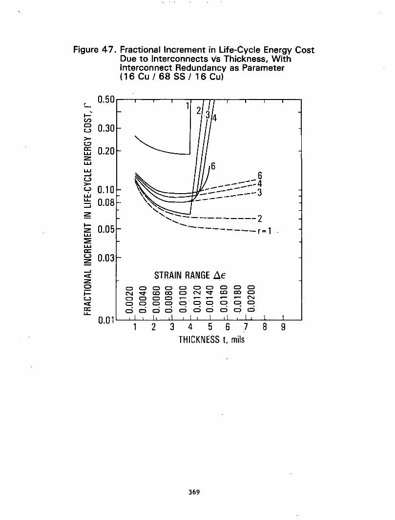
Figure 47. Fractional Increment in Life-Cycle Energy Cost Due to Interconnects vs Thickness, With Interconnect Redundancy as Parameter (16 Cu / 68 SS / 16 Cu)
0.50 L.
~
I-en a 0.30 u >-~ a:: 0.20 LU 2: LU
LU
6 .....J u --4 >-
0.10 -- --- --- ---u --:---- 3 . --...... ---LU ----u- 0.08 ---.....J
2:
I- 0.05 2: LU
:2: LU a:: u 0.03 z .....J
STRAIN RANGE Ll€ ex: 2: a a a a a a a a a a a l- N V co 00 a N v co 00 a u a a a a ..- ..- ..- ..- ..- N ex: a a a a 0'0 a a a a a:: a a oq a u- a a a a a
0.01 1 2 3 4 5 6 7 8 9
THICKNESS t, mils
369

Figure 48. Percentage of L~fe-Cycle Energy Cost Increment Due to Doubly Redundant Interconnects
1000
fii!
...: z w :!: w a: ~ z ~ CI) 0 ~
> t!:I
10 a: w Z w w ....... ~ > ~ w u.. =:i
a
STRAIN, !l€ 0.004 0.008 0.00 12
ALUMINUM 16 Cu/68 S8/16 Cu
COPPER
12.5 Cu/7!) INV/12.5 Cu
Figure 49. Conclusions
• Coppar IS a good interconnect material because of its low cost and high electrical conductivity
• Aluminum ranks poorly bacausa of its disappointing 'atlgua parformanca -
• Claddings offer improved performance due to substantially enhancad fatigue behavior; in particular. 33 Cu/33 INV/33 Cu exhibits superior overall pariormance
• Developed design algorithm provides an effective means of lISB888iag the econamil: merits of candidate interconnect matarials and module designs
370
6 7

Figure 50. Crack Propagation Across Fatigued Interconnect (12.5 Cu / 75 Inv / 12.5 Cu, Top View)
Figure 51 . Crack Propagation Across Fatigued Interconnect (12.5 Cu / 75 Inv / 12.5 Cu, Bottom View)
371

Figure 52. Crack Propagation Across Fatigued Interconnect (Annealed OFHC Copper, Top View)
37 2

Figure 53. Crack Propagation Across Fatigued Interconnect (Annealed OFHC Copper, Bottom View)
373

Figure 54. Schematic for Explaining Crack Propagation in Fatigued Interconnects
LESS HIGHLY STRESSED CONVEX SURFACE
~~ "" "'>.../, ....J" ___ ---" ......... _ v --"~ , ....... ~. ."."",.: ..... ~ r ~ .. ,.
374
NEUTRAl SURFACE AT FRACTURE
ORIGINAL NEUTRAl SURFACE

Figure 55. Neutral Surface at Fracture (1 2.5 Cu / 75 Inv / 1 2.5 Cu)
Figure 56. Tinned 1100 Aluminum Showing Region Between Aluminum and Tin
375

DISCUSSION
JOYCE: At the very end you made two comments about the copper-Invar system. In one case you said that the l2.S Cu/7S Inv/12.S Cu was economically favorable.
MON: No, the 33 Cu/33 Inv/33 Cu.
JOYCE: What was it you said about the 12.5 Cu/75 Inv/12.5 Cu, do you recall?
MON: I don't think I said anything about it really. It was less favorable. From a fatigue point of view the 12.5/75/12.5 is the best because it has more Invar in it than anything else and the Invar has much better fatigue characteristics than copper. But when you bring into account the costs, I2R, resistivity effects and everything else, the 33/33/33 turns out to be superior.
JOYCE: MY second question is about the copper. I notice that in each case you refer to the oxygen-free high-conductivity (OFHC) copper. How are its properties different from other copper available and what would be the disadvantage of using a non-OFHC copper for an interconnect?
MON: I don't know if I can totally answer that but OFHC copper, being pure, has the highest conductivity of any copper, so other than that I don't know what the advantage would be of using a less pure copper. Probably, if anything, it would be a disadvantage.
LEE: I may have missed it but did you have any environmental control on your test speclinens?
MON: No. They were tested in air. You saw that apparatus? They were mounted between those plates in air.
LEE: We, in conducting fatigue tests, have seen some influence of just the atmosphere on the resultant life, in particular crack-growth rates, depending on whether you use a nitrogen-purged atmosphere or just the normal amount of humidity that might exist in a laboratory environment. Just wondered if you had looked at this in any of your lifes?
MDN: No, we haven't. Our laboratory is humidity-controlled, more or less, and temperature-controlled, more or less. I have to say more or less because it isn't really controlled down to 10C or anything like that but we don't vary more than 20C during the course of the day even with a lot of equipment operating in there. We might go from 220C to 240C. I don't remember the humidity numbers but I think it is between 50% and 60%. 10 add a little dimension to your question, it should be noted that in actual use the interconnects themselves are encapsulated so atmospheric effects don't directly affect the interconnect operation. I know that water vapor does diffuse in and that all kinds of corrosion can happen. I have seen interconnect corrosion in modules in 850 -85% type humidity tests but we haven't taken that into account. We are strictly looking at one mechanism and that is thermal-cycle-induced mechanical fatigue.
376

MOORE: I think Gordon mentioned this in his talk but I want to emphasize that the module interconnect design influences where the strain range is
placed on the abscissa (thickness) of the graphs that he presented. The module design, I think, can influence the material selection.
MON: That's right. TO amplify that, you saw that at 2 mils thick, OFHC copper -- you suddenly got that big increase in life-cycle energy cost. That depends on the strain and what Don is saying is that depending on the design this strain can move back and forth on the X axis, which will likewise move all those curves back and forth.
OOuLBERT: One of the interconnect designs which has been used, and I am not ,sure wh~ther it is still in favor or not, is the expanded mesh that has been used on some modules. Is that still a viable design, and does your ,analys is include aspects of that problem?
MON: ,Whether or not it is a viable design, I don't know. I have not i~vestigated this. I have only looked at ribbon.
ROSS: ,I mignt point out that the algorithm is absolutely applicable as ~ong as you can calculate the strain in that thin mesh. Once you have calculated the strain in the algorithm it will carry you through to an answer as to whether it is cost-effective.
LANDEL: As some of my colleagues know, when I see a nice piece of work I am always one to p~sh it on a little bit further. In conjunction with the discussions which we have heard, then, vis-a-vis corrosion, the question has already been asked, but let's state it specifically: can you estimate how far your strain-versus-cycle (s-n) ~urves would shift with corrosion, or could someone in the audience shed some light on that?
MDN: I have no idea.
WHITE: In the work we have done with some of the modules, I have seen same extensive corrosion on our leads. They have discolored, they got really ugly-looking, but there was no obvious power loss due to that. The only power loss we have seen due to our leads was due to lead breakage caused by pulling too hard on them or something, actually breaking them.
LANDEL: Were these unencapsulated?
WHITE: They were encapsulated.
FEIGE: I assumed you selected the Invar because of its coefficient of expansion, am I correct?
MON: Yes.
FEIGE: I would complement you on the choice. I think you went the right way. I think you are getting enhanced protection with the Invar versus the copper.
MON: If you put the Invar on the outside like Invar/copper/Invar, instead of copper/Invar/copper, that might have a lot of advantages because the Invar would first of all resist fatigue better and it mignt have a better
377

corrosion resistance, because we are concerned with corrosion here. Although the copper/stainless/copper proved not be a good material, if you reversed that and made it stainless/copper/stainless you might begin to have a better perfotmance from the point of view'of fatigue resistance and corrosion.
FEIGE: OK. I'll buy that.
LEE: Just to follow up on the strain-versus-cycles (s~) curves: for corrodible material you would see a significant shift in the s-n curves, a significant degradation in the life at a given stress, and in the case of copper that might be the case. We haven't done any work in our lab. We have dealt primarily with steels and stainless steels but you can see an order of magnitude shift in life at a given stress in the presence of a corrosive environment. So you might have some conservative data, having generated the s-n curves in your laboratory air environment. If you looked at a cleaner environment which you might have in the encapsulation, you might actually see a longer life. In terms of the composites or the clad materials you have, if you have the Invar between the copper you may in fact have favorable galvanic relationships because you will have a small cathode and large anode. Similarly with the stainless clad on top of the copper you may have an inherently more corrosion-resistant material with the stainless steel on the surface. But if you do have any perforation of the stainless surface, then you will have very unfavorable relationships with large cathode areas with the stainless steel and very small anode areas with the copper where you have the perforation of the stainless steel. Which \vould lead to through-penetration.
MaN: Looking at the physical side of crack propagation, I think that the material will cycle for 90% of its life before a crack develops. The remaining 10% (and these are rough numbers) the crack will propagate. So I think corrosion would not be a problem because as long as the interconnect is encapsulated, 90% of its life will go by without experiencing much in the way of corrosive environment. Then when it does crack and water 9r what have you gets in, I don't think there is that much time left for the corrosion to really speed up the final failure. Am I wrong on that?
FEIGE: Corrosion fatigue will be quite a factor. It will rapidly accelerate the rate of failure.
MON: It is clear that we have done nothing on corrosion. We have talked about it a lot but it would be difficult to design this type of test. Fncapsulate a material and then shake it back and forth in a shaker. We could put it in a chamber. It's another thing to do.
378


