i

FATIGUE LIFE ESTIMATION OF A HIGHWAY SIGN STRUCTURE

by

Jennifer Ann Kacin

Bachelor of Science, University of Pittsburgh, 2007

Submitted to the Graduate Faculty of

Swanson School of Engineering in partial fulfillment

of the requirements for the degree of

Master of Science

University of Pittsburgh

2009

UNIVERSITY OF PITTSBURGH

SWANSON SCHOOL OF ENGINEERING

This thesis was presented

by

Jennifer Kacin

It was defended on

February 24, 2009

and approved by

Dr. Kent A Harries, Assistant Professor, Department of Civil and Environmental Engineering

Dr. John Brigham, Assistant Professor,

Department of Civil and Environmental Engineering

Dr. Piervincenzo Rizzo, Assistant Professor, Department of Civil and Environmental Engineering

Thesis Advisor

ii

Copyright © by Jennifer Kacin

2009

iii

FATIGUE LIFE ESTIMATION OF A HIGHWAY SIGN STRUCTURE

Jennifer Kacin, M.S.

University of Pittsburgh, 2009

Sign structures stand along every highway and interstate across the country in order to guide

motorists to their destination. Such structures are repeatedly subjected to natural wind gusts and

gusts from vehicles passing underneath. Over time, the members within the structure may begin

to succumb to fatigue due to this cyclical loading, in the form of cracks in the members and in

the connections. The goal of this project is to determine the fatigue life of an overhead four-

chord truss sign structure located in Pennsylvania in both a damaged and undamaged state. A

finite element model of the structure was made using commercial software and a time varying

natural wind load was applied to it. The stress history of critical elements was then extracted

from the model’s solution. Complete stress cycles were counted and then a linear damage

accumulation method was used in order to find the fatigue life in the critical members. The non-

damaged structure’s critical members were found to have an infinite fatigue, as were the

damaged structure’s critical members. Despite this, members with welded connections should

still be closely monitored during inspection because they have the highest potential for failure.

iv

TABLE OF CONTENTS

NOTATION ..................................................................................................................... XIII 

PREFACE ................................................................................................................................. XVI 

1.0  INTRODUCTION ........................................................................................................ 1 

1.1.1  Motivation ........................................................................................................ 1 

1.1.2  Project Goal...................................................................................................... 4 

1.1.3  Thesis Organization ......................................................................................... 7 

1.2  DISCLAIMER ..................................................................................................... 7 

2.0  LITERATURE REVIEW ............................................................................................ 8 

2.1  SUSCEPTIBILITY TO DAMAGE .................................................................... 8 

2.1.1  NCHRP Report 412 (1998) ............................................................................. 8 

2.1.2  AASHTO 2001 Specifications for Structural Supports ............................. 10 

2.1.3  NCHRP Report 494 (2003) ........................................................................... 10 

2.2  TRUCK INDUCED GUSTS ............................................................................. 12 

2.2.1  Creamer et al. (1979) ..................................................................................... 12 

2.2.2  Cook et al. (1997) ........................................................................................... 14 

2.2.3  NCHRP Report 412 (1998) ........................................................................... 14 

2.3  NATURAL WIND GUST DEVELOPMENT AND MODELING ................ 15 

2.3.1  NCHRP Report 412 (1998) ........................................................................... 15 

v

2.3.2  NCHRP Report 469 (2002) ........................................................................... 16 

2.3.3  Ginal (2003) .................................................................................................... 16 

2.3.4  Li (2005) .......................................................................................................... 17 

2.4  FATIGUE MODELING OF HIGHWAY SIGN STRUCTURES ................. 18 

2.4.1  Desantis and Haig (1996) .............................................................................. 18 

2.4.2  NCHRP Report 469 (2002) ........................................................................... 20 

2.4.3  Ginal (2003) .................................................................................................... 21 

2.4.4  Li (2005) .......................................................................................................... 23 

2.4.5  Park and Stallings (2006) .............................................................................. 24 

2.4.6  Discussion of Results of Past models ............................................................ 25 

2.5  INSPECTION .................................................................................................... 26 

2.5.1  Collins and Garlich (1997) ............................................................................ 26 

2.5.2  NCHRP Report 469 (2002) ........................................................................... 27 

2.5.3  Li (2005) .......................................................................................................... 28 

3.0  FINITE ELEMENT MODEL OF A 4 CHORD TRUSS ........................................ 29 

3.1  THE STRUCTURE ........................................................................................... 29 

3.2  THE FINITE ELEMENT METHOD .............................................................. 32 

3.3  BUILDING THE MODEL ................................................................................ 32 

3.3.1  Steps for Modeling ......................................................................................... 32 

4.0  WIND LOADING ON SIGN STRUCTURES ......................................................... 40 

4.1  DYNAMIC WIND LOADS .............................................................................. 40 

4.1.1  Galloping ........................................................................................................ 41 

4.1.2  Vortex Shedding ............................................................................................ 43 

vi

4.1.3  Truck Induced Gusts ..................................................................................... 45 

4.2  BASIC CHARACTERISTICS OF NATURAL WIND.................................. 46 

4.3  BLUFF BODY AERODYNAMICS ................................................................. 49 

4.3.1  Drag................................................................................................................. 50 

4.4  WIND SIMULATION ....................................................................................... 53 

4.4.1  The Davenport Spectrum .............................................................................. 54 

4.4.2  The Kaimal Spectrum ................................................................................... 55 

4.4.3  Analytical Wind Simulation Process ........................................................... 56 

4.5  CONCLUSION .................................................................................................. 61 

5.0  FATIGUE LIFE CALCULATION .......................................................................... 62 

5.1  INTRODUCTION ............................................................................................. 62 

5.2  FATIGUE ........................................................................................................... 63 

5.3  THE AASHTO STRESS LIFE METHOD ...................................................... 64 

5.3.1  Rainflow Counting Algorithm ...................................................................... 66 

5.3.2  Member End Connections ............................................................................ 70 

5.3.3  Fatigue Limits ................................................................................................ 73 

5.3.4  The Palmgren-Miner Rule of Linear Damage Accumulation ................... 75 

5.4  FATIGUE LIFE ANALYSIS ............................................................................ 77 

5.4.1  Wind Probability ........................................................................................... 77 

5.4.2  Example Calculation ..................................................................................... 83 

5.4.3  Results ............................................................................................................. 88 

5.5  CONCLUSION .................................................................................................. 91 

6.0  FATIGUE LIFE OF A DAMAGED SIGN .............................................................. 92 

vii

6.1  SIMULATION ................................................................................................... 92 

6.1.1  Results ............................................................................................................. 94 

6.2  CONCLUSION .................................................................................................. 97 

7.0  CONCLUSION ........................................................................................................... 98 

7.1  DISCUSSION ..................................................................................................... 98 

7.2  FUTURE WORK ............................................................................................. 100 

APPENDIX A ............................................................................................................................ 101 

APPENDIX B – SIMULATION FILES ................................................................................. 105 

APPENDIX C – AASHTO FATIGUE DETAIL TABLE ..................................................... 120 

BIBLIOGRAPHY ..................................................................................................................... 124 

viii

LIST OF TABLES

Table 2-1 Design Pressures from Cook et al. (1997) .................................................................... 14 

Table 2-2 Expected fatigue life from Ginal (2003) ...................................................................... 22 

Table 3-1 Modal frequencies (in Hz) for the first 10 mode shapes .............................................. 36 

Table 4-1AASHTO coefficients of drag for sign panels (AASHTO, 2001) ................................ 51 

Table 4-2 Modeled sign coefficients of drag ................................................................................ 51 

Table 4-3 Wind speed frequencies for Pittsburgh, Pa ................................................................... 57 

Table 5-1 Connection Details and there locations within the structure ........................................ 72 

Table 5-2 Critical element stress categories ................................................................................. 73 

Table 5-3 Constant amplitude fatigue limits (AASHTO, 2001) ................................................... 75 

Table 5-4 Conditional Probabilities (P(A|B)) for A = wind speed and B = wind direction ......... 81 

Table 5-5 Joint Probabilities (P(A∩B)) for A = wind speed and B = wind direction .................. 81 

Table 5-6 Conditional Probabilities (P(A|B)) for A = wind direction and B = wind speed ......... 82 

Table 5-7 Joint Probabilities (P(A∩B)) for A = wind direction and B = wind speed .................. 82 

Table 5-8 ANSYS element numbers corresponding to Figure 5-12 ............................................. 84 

Table 5-9 Stress ranges in psi in element 1921 at 25 mph............................................................ 85 

Table 5-10 The damage at node i and j of element 1921 caused by a 25 mph wind .................... 86 

Table 5-11 Probability of wind blowing in a certain direction for a certain speed ...................... 87 

ix

Table 5-12 Number of 5 second cycles per year for given direction and speed ........................... 87 

Table 5-13 Fatigue life calculation for node i of element 1921 at 25 mph ................................... 88 

Table 5-14 Fatigue life for the four sign model ............................................................................ 89 

Table 5-15 Fatigue life for the five sign model ............................................................................ 90 

Table 6-1 Fatigue life with 1 element damaged ............................................................................ 95 

Table 6-2 Fatigue life with 2 elements damaged .......................................................................... 95 

Table 6-3 Fatigue Life when Critical element 1926 is damaged .................................................. 96 

Table 6-4 Reduction in Fatigue life .............................................................................................. 96 

Table A-7-1 Model information .................................................................................................. 101 

x

LIST OF FIGURES

Figure 1-1 Collapse of cantilevered structure along I-65 in Tennessee .......................................... 3 

Figure 1-2 a. Structure mounted sign b. Free standing VMS c. Single cantilevered pole d. Double cantilevered pole e. Overhead monotube f. Overhead 2 chord truss g. Overhead trichord truss ..................................................................................................................................... 6

Figure 2-1 Proposed truck gust on a sign structure (Creamer et al. 1979) ................................... 13 

Figure 2-2 Structure analyzed in Desantis and Haig (1996) ......................................................... 18 

Figure 3-1 Sign structure 511-76 in Allegheny County. View while traveling (a) north and (b) south (Courtesy of the Pennsylvania Department of Transportation) .............................. 30

Figure 3-2 Sign attachments as shown on plans ........................................................................... 31 

Figure 3-3 ANSYS model of sign structure 511-76. (a) Model with 4 aluminum signs attached. (b) Model with 5 aluminum signs attached....................................................................... 34

Figure 3-4 First four mode shapes in the pinned base case. ......................................................... 37 

Figure 3-5 First four mode shapes in the fixed base case ............................................................. 38 

Figure 3-6 Connection of flat panel sign to truss .......................................................................... 39 

Figure 4-1 A non-periodic wind loading ...................................................................................... 41 

Figure 4-2 Galloping of a cantilevered structure (FHWA 2005) .................................................. 42 

Figure 4-3 Vortex Shedding (FHWA 2005) ................................................................................. 44 

Figure 4-4 Shedding of vortices on a bluff body .......................................................................... 45 

Figure 4-5 Wind speed Vs time (adapted from Liu 1991) ............................................................ 47 

Figure 4-6 Comparison of Logarithmic and Power law (adapted from Holmes 2007) ............... 48 

xi

Figure 4-7 Wind flow around a streamlined and bluff body (Holmes 2007) ............................... 49 

Figure 4-8 Typical spectrum of wind turbulence S1 or S2 as a function of frequency n (Liu 1991) ................................................................................................................................. 53

Figure 4-9 The Davenport spectrum fitted to the studied data (Davenport 1960) ........................ 55 

Figure 4-10a Wind pressures to be applied to signs ..................................................................... 60 

Figure 4-10b Wind pressures to be applied to truss elements ...................................................... 60 

Figure 5-1 Steps in a fatigue life calculation (Ariduru, 2004) ...................................................... 62 

Figure 5-2 AASHTO Stress-Life curve (AASHTO 2004) ........................................................... 65 

Figure 5-3 Locations of critical elements ..................................................................................... 67 

Figure 5-4 Rainflow counting using the ASTM algorithm (adapted from Bannantine 1990)...... 68 

Figure 5-5 Flow chart of rainflow counting algorithm steps ........................................................ 69 

Figure 5-6 Location of connection details within the structure ................................................... 71 

Figure 5-7 Frequency of wind speeds in Pittsburgh, Pa ............................................................... 78 

Figure 5-8 Frequency of wind direction in Pittsburgh, Pa ............................................................ 78 

Figure 5-9 Directional Probabilities given that a certain wind speed has occurred ...................... 80 

Figure 5-10 Critical elements at the left and right end ................................................................. 83 

Figure 5-11 Stress time history for element 1921 at a base speed of 25 MPH ............................. 84 

Figure 6-1 Member with a reduced capacity ................................................................................ 93 

Figure 6-2 2 members with reduced capacity ............................................................................... 93

xii

NOTATION

Abbreviations

AASHTO American Association of State Highway and Transportation Officials

APDL ANSYS Parametric Design Language

ASTM American Society for Testing and Materials

CAFL Constant Amplitude Fatigue Limit

DOT Department of Transportation

FHWA Federal Highway Administration

LCD Local Climate Data

NCDC National Climate Data Center

NCHRP National Cooperative Highway Research Program

VAFL Variable Amplitude Fatigue Limit

VMS Variable Message Sign

Notation

A Area

A AASHTO constant

Cd Coefficient of Drag

Cdδ Reduced drag coefficient

D Damage

F(t) Force as a function of time

xiii

fk Frequency

k von Karmen constant

Kp Porosity factor

n Frequency

N Number of cycles to failure

P(t) Pressure as a function of time

pa Ambient Pressure

ps Stagnation Pressure

S Stress

Sd Power Spectrum

Sk Kaimal spectrum value

Ska Power Spectrum

t Time

u* Shear velocity

Uz Mean wind velocity at a reference height

v(z) Wind speed

V* Shear velocity

v’(t) Turbulent wind Speed

z Height above ground

z0 Effective height above ground

α Power law exponent

δ Solidity ratio

ρ Air density

xiv

φk Random Phase angle between 0 and 2π

 

xv

xvi

PREFACE

I would like express my thanks to Dr. Piervincenzo Rizzo for his guidance in this research

project. His motivation for me kept me going and he played a key part in getting this document

into its final form. I want to thank him for all of his time and input on this project.

I would also like to thank Dr. John Brigham and Dr. Kent Harries for serving on my

thesis defense committee. Dr. Brigham’s knowledge of computer modeling was essential in the

completion of this project. Dr. Harries has been instrumental the development of my skills in

structural design and analysis which was incredibly helpful throughout all of my research and

will serve me well in my future career.

I must thank Mr. David Schmidt for the guidance he provided in the use of ANSYS.

Without him I would probably still be lost. Additionally, I would like to thank Mr. Frank

Kremm for quickly providing me with tech support on what was at least a monthly basis.

Thanks to Mr. Jerry Bruck of PennDOT for providing the necessary documents and

pictures along with assistance on this project.

I would like to thank my Peers Mr. Jarret Kasan, Mr. Antonino Spada, Mr. Venu Gopal

Annamdas, Mr. Xuan Zhu, and Mr. Xiangli Ni for their help and support on this project.

Lastly, I would like to thank my parents and extended family for all of their love, support

and encouragement. I could never have gotten here without them and I owe them the world.

1.0 INTRODUCTION

1.1.1 Motivation

Overhead and bridge sign support structures can be found along any major highway across the

United States. These structures support signage that helps commuters navigate their way.

Highway sign structures are multi degree of freedom (MDOF) systems that come in many

different shapes and sizes. The signage consists either of standard aluminum flat signs or

variable message signs (VMS). Types of sign structures range from a single pole cantilevered

over the highway to a four chord truss structure spanning several lanes of traffic.

Cantilevers are made of a mast arm extending out over the roadway supported by a single

roadside column, typically a single or double pole or a box-truss structure. The vertical columns

are referred to as uprights, posts, or poles. The horizontal part of the structure is referred to as the

mast arm (usually in reference to a monotube, that is a single tube without joints), the truss (for

other than monotubes), or the cantilever.

In the fourth edition of the Standard Specifications for Structural Supports for Highway

Signs, Luminaires, and Traffic Signals (AASHTO 2001), structures supported on both sides of

the roadway are referred to as bridge supports. Bridge supports are also called span-type

structures, sign bridges, or overhead structures (although this latter term is sometimes used to

describe both cantilever and bridge supports) (Dexter and Ricker 2002). The roadside columns

1

that support the mast range from single poles to box-truss structures. Vertical uprights can form

a truss that is composed of two chord members braced by web members using similar member-

to-member connections as in the overhead truss-type structure.

Cantilevered support structures can be an attractive option because the cost is typically

less than 40 percent of the cost of bridge supports. Also, the single upright increases motorist

safety by reducing the probability of vehicle collision (Dexter and Ricker 2002).

During the past two decades, these simple structures have shown underlying problems

associated with their reduced fatigue performance. Defective welds, aging material, and harsh

environmental conditions (particularly wind loading) have exacerbated these problems. In

general, highway sign supports must withstand in-service dynamic loads, which constitute the

fatigue environment. Sources of these loads include natural winds, artificial gusts created by

passing vehicles, and vibrations induced into bridges by passing vehicles (for sign supports

mounted on a bridge). Most of the underlying problems involve cracks induced into welds by

fatigue loading. Generally, cracks are found propagating within a fillet weld or at the toe.

Depending upon the amount of time the crack has had to grow, these cracks can propagate into

the main supporting member (e.g., the chord of a truss).

While identifying cracks in these structures is the first step in addressing the problem,

determining the residual lifetime will lead to an optimal cost solution (repair, retrofit, or

replacement), especially if the crack is identified at an early stage before it has propagated into

the supporting member. The failure of these sign structures may cause traffic delays or car

accidents that can lead to serious injuries.

In the past year alone there have been at least 2 sign structure failures. On October 5,

2008 a drunk driver skidded sideways into an overhead sign support structure on Route 1 in

2

North Carolina causing it to collapse (Driver 2008). On July 7, 2008 a cantilevered structure on

I-65 in Tennessee fell onto the highway due to a crack at the base of the support pole, as seen in

Figure 1-1. TDOT’s early investigation indicates that prolonged exposure to gusts may have

caused this failure (Finley 2008). Additionally, excessive vibration due to wind gusts has been

documented in both New Jersey and Florida (Johns and Dexter 1998).

In order to avoid a situation like that seen in Figure 1-1, the American Association of

State Highway and Transportation Officials (AASHTO) lists four types of wind fatigue design

loads in the 2001 Standard Specifications for Structural Supports for Highway Signs, Luminaries

and Traffic Signals: galloping, vortex shedding, natural wind gusts, and truck induced gusts (also

known as buffeting).

Figure 1-1 Collapse of cantilevered structure along I-65 in Tennessee

These four are included in order to “avoid large-amplitude vibrations and to preclude the

development of fatigue cracks in various connection details and at other critical locations”

(AASHTO 2001). A basic definition as given in the AASHTO 2001 specifications for each of

these wind loadings and phenomena is:

• Galloping – results in large amplitude, resonant oscillations in a plane normal to the direction

of wind flow.

3

• Vortex Shedding – Structural elements exposed to steady, uniform wind flows will shed

vortices in the wake behind the element. When the frequency of vortex shedding approaches

the natural frequency of the structure, significant amplitudes of vibration can be caused in a

plane normal to the direction of wind flow.

• Natural Wind Gusts – The changing nature of the direction and magnitude of wind flow

against a sign structure can induce vibrations in the structure.

• Truck Induced Gusts – As trucks pass beneath sign structures they may induce gusts on the

attachments mounted to the structure. Loads are induced in both the horizontal and vertical

directions, but those in the vertical direction are much more critical.

1.1.2 Project Goal

The aim of the research presented in this thesis is to develop a finite element model for an

overhead sign structure in order to: a) determine the effect of wind loads on the fatigue

performance; b) identify the elements of the structure prone to fatigue cracking; c) establish a

relationship between damage severity and residual fatigue lifetime. This was done by performing

the following steps:

1. Review the algorithms utilized to model the action of wind on structures;

2. review the fatigue theories applied to dynamic analysis to determine residual fatigue life of

structures;

3. formulate an accurate loading scenario that sign structures are subjected to while in service;

4. identify the elements of the structures more prone to develop fatigue cracks;

5. calculate the fatigue life of the critical elements under pristine conditions of the sign

structures;

4

6. calculate the fatigue life of the critical elements in the presence of simulated damaged

conditions.

In particular, steps 3 to 6 were accomplished by examining a real structure in the

Commonwealth of Pennsylvania. The damaged scenario was modeled by reducing the material

elastic properties of some components within the structure.

Fatigue failure can be identified as a structural failure under a repeated loading. It is not

caused by one application of loading, but rather by several over a period of time. Fatigue may

occur as either low-cycle or high cycle fatigue (Pun 2001). In low-cycle fatigue, there are large

cycles that cause plastic deformation and lead to a short life. Conversely, in high cycle fatigue

stress cycles occur in the elastic range. They are caused by low loads and allow for a longer life.

High cycle fatigue takes place in highway sign structures.

As a part of the study, a survey was sent to all state DOTs and all of the districts within

PennDOT to inquire about the most common problems observed in sign structures. Frequent

problems include cracks in welds between members, corrosion, and loose or missing bolts.

Cracks can be caused by fatigue and corrosion. Either cracks or missing bolts can shorten a

structure’s fatigue life, which can be defined as the number of stress cycles that a member may

sustain before failure occurs (Stephens 2000).

The response of the PennDOT districts to this survey found that the following types of

sign structures are used in Pennsylvania: overhead truss with single pole supports, overhead truss

with truss supports, cantilever with single pole, cantilever with double pole, monotube, pole

mounted VMS, and structure mounted signs. These types of signs structures are shown in Figure

1-2.

5

f.

Figure 1-2 a. Structure mounted sign b. Free standing VMS c. Single cantilevered pole d. Double cantilevered pole

e. Overhead monotube f. Overhead 2 chord truss g. Overhead trichord truss

6

1.1.3 Thesis Organization

Chapter 2 presents a literature review of past research related to fatigue in sign structures. This

includes their susceptibility to damage, truck induced gusts, and natural wind gusts, along with

past efforts which used finite element modeling to aid in fatigue life prediction, and the state of

inspection of sign structures. Chapter 3 presents the sign structure and finite element model used

in this study. Chapter 4 details the different wind loadings that act on sign structures. It also

explains how the natural wind load history that is used in this project was developed. Chapter 5

explains the fatigue life evaluation method and provides an example of a how the fatigue life of a

critical member is calculated. Chapter 6 gives the results of fatigue life of the structure with the

added consideration that the structure has already been damaged. Lastly, chapter 7 presents the

conclusions of this research.

1.2 DISCLAIMER

This document presents a method to predict fatigue life for members in a structure. Use of the

results or reliance on the material presented is the responsibility of the reader. The contents of

this document are not meant to be a standard way to perform these calculations and are not

intended for use as a reference in specifications, contracts, regulations, statutes, or any other

legal document. The opinions and interpretations expressed are those of the author and other

duly referenced sources. The views and findings reported herein are solely those of the writers

and not necessarily those of PennDOT. This report does not constitute a standard, specification,

or regulations.

7

2.0 LITERATURE REVIEW

This chapter will present the findings of previous research on highway sign support structures.

The National Cooperative Highway Research Program (NCHRP) has released several reports to

support the American Association of State Highway and Transportation Officials (AASHTO)

standard design guidelines for sign support structures. Along with these reports, several other

researchers have studied different aspects of fatigue in such structures. The review is organized

by outlining: 1) the mechanisms that induce damage; 2) the effects of truck induced loads and

natural wind gusts; 3) the past models used to simulate fatigue; 4) the inspection techniques

adopted to detect damage.

2.1 SUSCEPTIBILITY TO DAMAGE

2.1.1 NCHRP Report 412 (1998)

Several occurrences of excessive vibration or even collapse in highway sign structures led the

NCHRP to issue report 412. These problems made it clear that the 1994 AASHTO (AASHTO

1994) specifications on fatigue and vibration in sign structures needed to be reevaluated. The

goals of the authors (Kaczinski et al. 1998) were to characterize the susceptibility of cantilevered

structures to excessive displacement or fatigue damage, to develop equivalent static load ranges

8

for the four common wind related causes of fatigue, to identify the fatigue sensitive connection

details in a sign structure, and to determine the fatigue strength of anchor bolts.

In order to determine the susceptibility to galloping and vortex shedding the authors

undertook wind tunnel testing of scale models of five representative structures. Three of the

structures were cantilevered mast arms (one supporting two traffic lights, one supporting one

traffic light, and one with a sign) while the others were two chord trusses (both supporting a

single sign). The structures were tested with and without the sign attachments. It was found that

galloping induced vibrations depend on the condition of the specific structure and do not occur

frequently, but once they do occur vibration can persist. The authors recommended that a shear

pressure range of 21 psf (1000 Pa) be applied vertically to the vertically projected area of any

attachment when designing for galloping of cantilevered structures. The authors reported that

overhead structures are likely not susceptible to galloping. In regards to vortex shedding, they

found that it only needs to be considered before the attachments (such as signs or lights) are

attached to the structure and that only structures with horizontal supports of large diameter are

prone to such phenomena.

A second goal of the research was to categorize the fatigue sensitive connection details

with respect to the AASHTO fatigue design curves (AASHTO 1994). They grouped together

those details with similar cracking modes and similar stress concentrations into categories A-E’

where the fatigue threshold of the detail decreases as you move from letter A to letter E’. The

majority of details on a cantilevered sign were put into the E or E’ category, though anchor bolts

were put into category D.

9

2.1.2 AASHTO 2001 Specifications for Structural Supports

The fatigue chapter of the AASHTO 1994 structural supports specifications was updated based

on the recommendations of NCHRP report 412 and contains provisions for the fatigue design of

cantilevered steel structural supports. These supports should be designed for fatigue due to loads

from galloping, natural wind gusts, and truck induced wind gusts. The commentary in the

AASHTO 2001 structural support manual provides extra information in regards to designing for

fatigue: galloping results in large amplitude, resonant oscillations in a plane normal to the

direction of wind flow, and is usually limited to structures with a nonsymmetrical cross section;

in the case of the four chord horizontal truss, the owner may choose to exclude galloping loads.

The AASHTO structural supports manual also states that truck gust pressures are applied only to

the exposed horizontal attachment and horizontal support, but may also be excluded from design

as allowed by the owner.

AASHTO recommends the use of the stress life method and the use of an infinite life

design based on the Constant Amplitude Fatigue Limit (CAFL). The CAFL is the value of the

portion of the SN curve with zero slope. All structures with stresses below the CAFL are

considered to have an infinite life. These concepts will be detailed in Chapter 5.

2.1.3 NCHRP Report 494 (2003)

NCHRP Report 494 “Structural Supports for Highway Signs, Luminaries, and Traffic Signals”

was released in 2003 (Fouad et al. 2003). Prior to this report most research done on highway

sign structures focused on cantilevered structures. The work of Fouad and co-authors studied

fatigue and vibration in overhead structures and aimed to recommend a set of fatigue loads. Part

10

of the work included the release of a survey to all state DOTs, and out of 48 responses, 8

indicated problems with non-cantilevered structures. The report included a proposed connection

design detail to minimize fatigue effects, an evaluation of the effectiveness of gussets in reducing

fatigue problems, and proposed vibration mitigation methods.

Several loading recommendations came out of this report:

1. Galloping – A 21 psf pressure applied vertically to the projected area of the signs

mounted to monotube support structures as viewed in the normal elevation.

Galloping will only apply to horizontal monotubes. Non-cantilevered structures

and truss type supports are excluded.

2. Vortex Shedding – this design requirement may be disregarded as long as the signs or

sign blanks are used during construction.

3. Natural wind loads – 5.2 psf multiplied by the drag coefficient applied in the horizontal

direction to the exposed area of all support structure members, signs, and

attachments.

4. Truck induced loads – 7.5 psf for the horizontal pressure applied to the area of the sign

and the area of the support structures, and 10.2 psf for the vertical pressure

applied to the area of the support structure and the projected area of the sign.

These pressures should be applied along the smaller of 24 feet or the entire span.

A few other recommendations came out of this report. For example, gusset plates were

recommended to increase the moment capacity of connections. Despite the research done for

this report, it was still unclear as to whether or not non-cantilevered sign structures are

susceptible to fatigue from galloping and vortex shedding. The author said that more field

testing needed to be done in order to draw any conclusions.

11

2.2 TRUCK INDUCED GUSTS

2.2.1 Creamer et al. (1979)

A method for designing cantilevered signs in the presence of truck gust loading was

developed. More specifically, the authors aimed to determine the fatigue load produced by such

a loading by performing both analytical and experimental work. Three structures were

instrumented with strain gages and the researchers found that the magnitude of the mast arm

response varied depending on the truck’s shape and speed. The field research was also

performed in order to determine the member forces in the structure due to truck induced gust

loads.

Actual gust forces were not measured for the development of a truck gust loading

function. Instead, the loading function was developed analytically by examining the member

force ratios that resulted from various loading function shapes. These ratios were compared with

experimental data in order to find the correct function.

Experimental tests showed that trucks produce gusts in both the horizontal and vertical

direction. The vertical gust is caused by upward deflection by the cab, and the peak pressure

occurs at some point behind the back of the cab. The horizontal gust is the result of suction

pressure, and is a function of the truck’s frontal area. It also depends on the truck’s length,

contour, roughness, and velocity. The pressure loading function developed in this research is

shown in Figure 2-1. This loading is not presumed to be the actual gust loading that is present in

the field. Instead, it was developed to simulate the member forces that were measured

analytically.

12

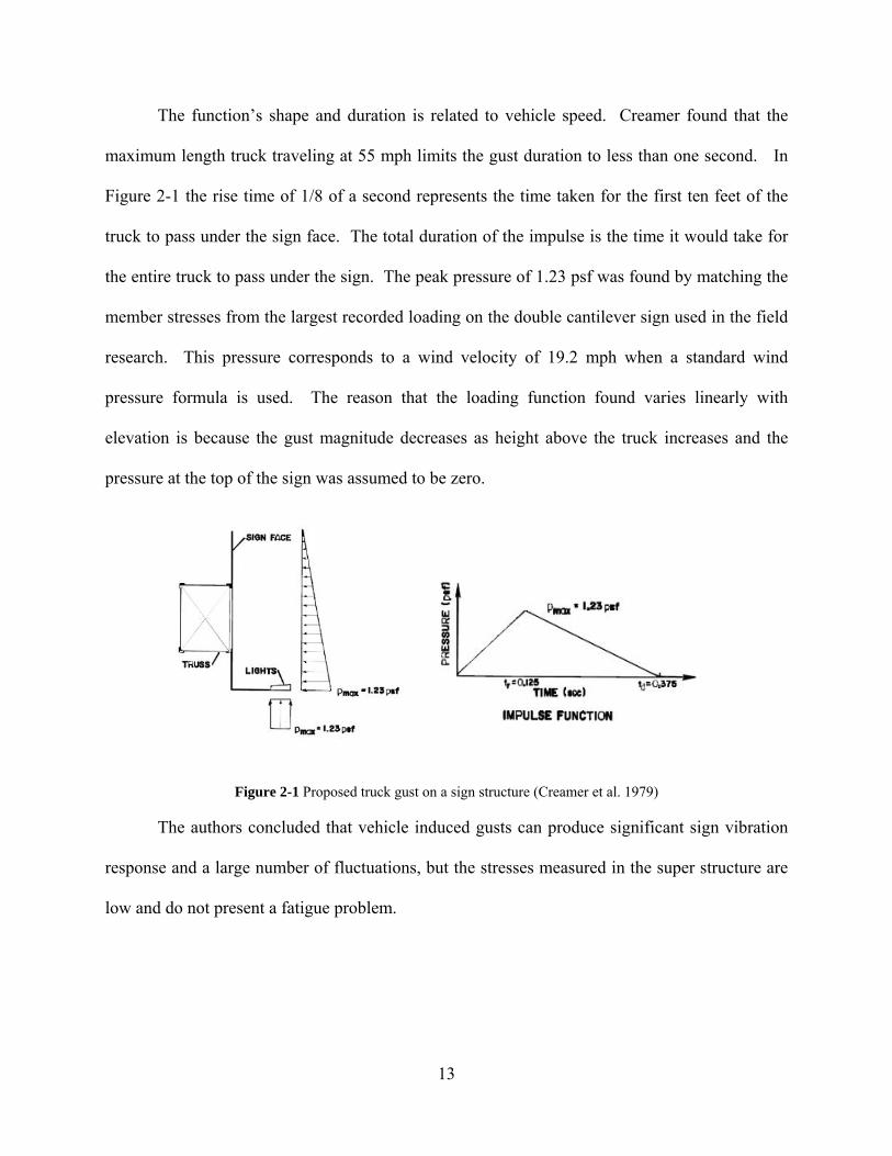
The function’s shape and duration is related to vehicle speed. Creamer found that the

maximum length truck traveling at 55 mph limits the gust duration to less than one second. In

Figure 2-1 the rise time of 1/8 of a second represents the time taken for the first ten feet of the

truck to pass under the sign face. The total duration of the impulse is the time it would take for

the entire truck to pass under the sign. The peak pressure of 1.23 psf was found by matching the

member stresses from the largest recorded loading on the double cantilever sign used in the field

research. This pressure corresponds to a wind velocity of 19.2 mph when a standard wind

pressure formula is used. The reason that the loading function found varies linearly with

elevation is because the gust magnitude decreases as height above the truck increases and the

pressure at the top of the sign was assumed to be zero.

Figure 2-1 Proposed truck gust on a sign structure (Creamer et al. 1979)

The authors concluded that vehicle induced gusts can produce significant sign vibration

response and a large number of fluctuations, but the stresses measured in the super structure are

low and do not present a fatigue problem.

13

2.2.2 Cook et al. (1997)

The magnitude, direction, and frequency of pressure distributions on VMS caused by trucks

passing underneath were determined. A pressure monitor was placed on a VMS mounted on a

bridge overpass and data were collected as trucks passed. The monitor was designed so that its

height above the ground could be adjusted based on the researcher’s needs. The events of 23

random trucks passing with the monitor at a height of 17 feet were observed. It was found that

the truck induced gusts caused both negative and positive pressure as they passed and that the

maximum positive pressure occurred at an angle of 75º to the front of the sign while the

maximum negative pressure occurred normal to the sign face. The overall pressure readings

ranged between -1.5 psf to 1.5 psf.

In order to find the effect of height on pressure, Cook and co-authors drove a rented

semitrailer truck with an unspecified height at a constant speed of 65 mph underneath with the

monitor mounted at heights of 17, 18, 19, and 20 feet above the roadway. A 10% reduction in

pressure for each foot of sign elevation increase was observed. Table 2-1 shows the final design

pressures determined in this work.

Table 2-1 Design Pressures from Cook et al. (1997)

Bottom Horizontal Surface (0º)

Leading Vertical Surface (90º)

Positive pressure (psf) 0.92 1.43 Negative Pressure (psf) -1.50 -2.10

2.2.3 NCHRP Report 412 (1998)

Kaczinski et al. (1998) based their work to find a static pressure range for truck induced loads on

functions proposed by Creamer et al (1979). They performed field tests which resulted in stress

14

ranges below that which would cause fatigue damage. They noted that failures had occurred in

Virginia, and concluded that the method proposed by Creamer does not produce accurate results.

In the next model, it was assumed that the velocity of the upward gust is equal to the velocity of

the truck. Because head winds could increase the relative truck speed, the authors added a gust

factor of 1.3 to the formula in the specification. They then doubled the obtained pressure to

represent the fact that during one cycle the cantilevered arm will move both downward and

upward. They found a value of 1760 Pa (36.6 psf) to be appropriate to use as an equivalent

vertical static pressure.

2.3 NATURAL WIND GUST DEVELOPMENT AND MODELING

2.3.1 NCHRP Report 412 (1998)

Kaczinski et al. (1998) studied equivalent static pressures generated by natural wind that could

be used for fatigue design calculations. Spectral analysis was used to model the response of a

cantilevered support structure to natural wind. It was important to do this accurately because if

galloping in a structure can be mitigated then natural wind gust will govern the fatigue design of

a sign structure. A fluctuating wind force was characterized as a random process and was

applied to exposed areas of the structure. In order to derive the wind force spectrum, the authors

used the Davenport wind velocity spectrum (Davenport 1961a). The wind loading was then

considered as a stationary mean velocity with a 1 hour period and the Davenport spectrum was

used with a range of these mean velocities as the input.

15

Four different types of cantilevered structures were analyzed using a finite element

process and the previously described wind loads. The effective stress ranges as a function of the

mean hourly velocity were found at critical fatigue details. An equivalent static pressure was

then found for each structure and these four values were averaged to equal a proposed value of

5.2 psf (250 Pa). This value was later adopted in the AASHTO 2001 sign support specifications.

To account for the structure that the wind is applied to the 5.2 psf (250 Pa) must be multiplied by

a coefficient of drag and an importance factor because these values vary depending on the

geometry of the signs and structure.

2.3.2 NCHRP Report 469 (2002)

Dexter and Ricker (2002) sought to verify a natural wind gust pressure equation that the

authors of the earlier NCHRP report 412 formulated. They developed several finite element

models (which will be discussed later in this literature review) to which they applied a randomly

occurring wind load. Base wind speeds within the range of 0-60 mph were deemed sufficient

because extreme speeds with a mean occurrence of greater than 1 year are not necessary in a

fatigue analysis. The Davenport velocity spectrum was used in this research to find the

fluctuating component of wind and the entire random response was represented by a series of

sinusoidal waves.

2.3.3 Ginal (2003)

Ginal also modeled a time history of randomly varying wind speeds to be applied to the finite

element models of three overhead sign structures. A wide range of mean wind speeds (5-50

16

mph) were used in the analysis and a fluctuating component of wind was modeled using the

Kaimal wind spectrum (Kaimal et al. 1972). This was chosen because unlike the Davenport

spectrum used in Dexter and Ricker (2002) the Kaimal spectrum takes elevation into account.

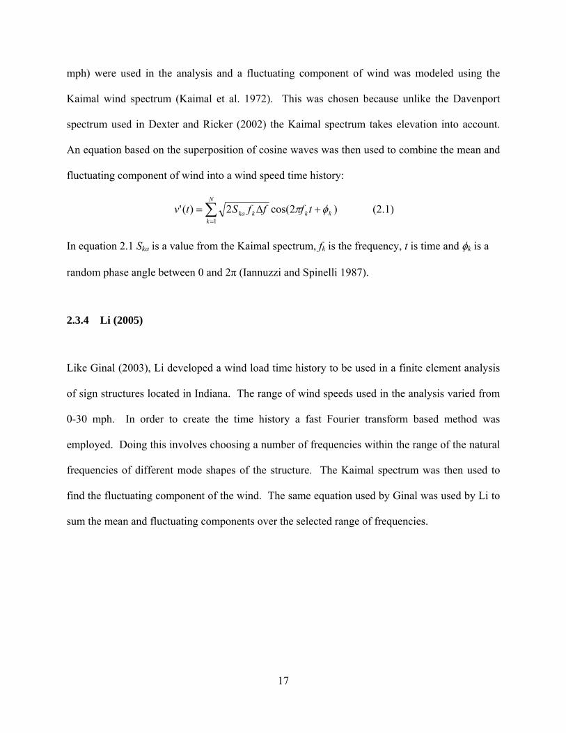
An equation based on the superposition of cosine waves was then used to combine the mean and

fluctuating component of wind into a wind speed time history:

∑=

+Δ=N

kkkkka tfffStv

1)2cos(2)(' φπ (2.1)

In equation 2.1 Ska is a value from the Kaimal spectrum, fk is the frequency, t is time and φk is a

random phase angle between 0 and 2π (Iannuzzi and Spinelli 1987).

2.3.4 Li (2005)

Like Ginal (2003), Li developed a wind load time history to be used in a finite element analysis

of sign structures located in Indiana. The range of wind speeds used in the analysis varied from

0-30 mph. In order to create the time history a fast Fourier transform based method was

employed. Doing this involves choosing a number of frequencies within the range of the natural

frequencies of different mode shapes of the structure. The Kaimal spectrum was then used to

find the fluctuating component of the wind. The same equation used by Ginal was used by Li to

sum the mean and fluctuating components over the selected range of frequencies.

17

2.4 FATIGUE MODELING OF HIGHWAY SIGN STRUCTURES

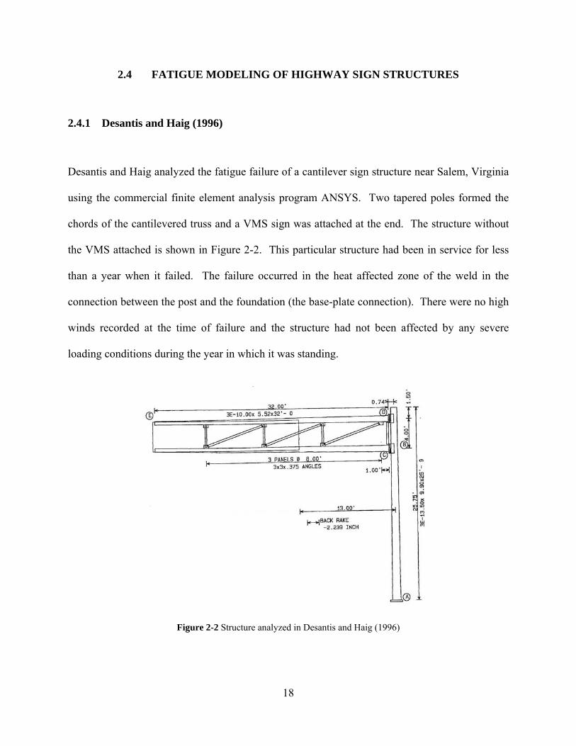
2.4.1 Desantis and Haig (1996)

Desantis and Haig analyzed the fatigue failure of a cantilever sign structure near Salem, Virginia

using the commercial finite element analysis program ANSYS. Two tapered poles formed the

chords of the cantilevered truss and a VMS sign was attached at the end. The structure without

the VMS attached is shown in Figure 2-2. This particular structure had been in service for less

than a year when it failed. The failure occurred in the heat affected zone of the weld in the

connection between the post and the foundation (the base-plate connection). There were no high

winds recorded at the time of failure and the structure had not been affected by any severe

loading conditions during the year in which it was standing.

Figure 2-2 Structure analyzed in Desantis and Haig (1996)

18

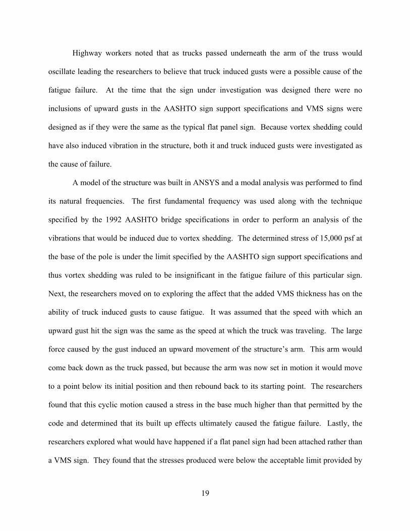
Highway workers noted that as trucks passed underneath the arm of the truss would

oscillate leading the researchers to believe that truck induced gusts were a possible cause of the

fatigue failure. At the time that the sign under investigation was designed there were no

inclusions of upward gusts in the AASHTO sign support specifications and VMS signs were

designed as if they were the same as the typical flat panel sign. Because vortex shedding could

have also induced vibration in the structure, both it and truck induced gusts were investigated as

the cause of failure.

A model of the structure was built in ANSYS and a modal analysis was performed to find

its natural frequencies. The first fundamental frequency was used along with the technique

specified by the 1992 AASHTO bridge specifications in order to perform an analysis of the

vibrations that would be induced due to vortex shedding. The determined stress of 15,000 psf at

the base of the pole is under the limit specified by the AASHTO sign support specifications and

thus vortex shedding was ruled to be insignificant in the fatigue failure of this particular sign.

Next, the researchers moved on to exploring the affect that the added VMS thickness has on the

ability of truck induced gusts to cause fatigue. It was assumed that the speed with which an

upward gust hit the sign was the same as the speed at which the truck was traveling. The large

force caused by the gust induced an upward movement of the structure’s arm. This arm would

come back down as the truck passed, but because the arm was now set in motion it would move

to a point below its initial position and then rebound back to its starting point. The researchers

found that this cyclic motion caused a stress in the base much higher than that permitted by the

code and determined that its built up effects ultimately caused the fatigue failure. Lastly, the

researchers explored what would have happened if a flat panel sign had been attached rather than

a VMS sign. They found that the stresses produced were below the acceptable limit provided by

19

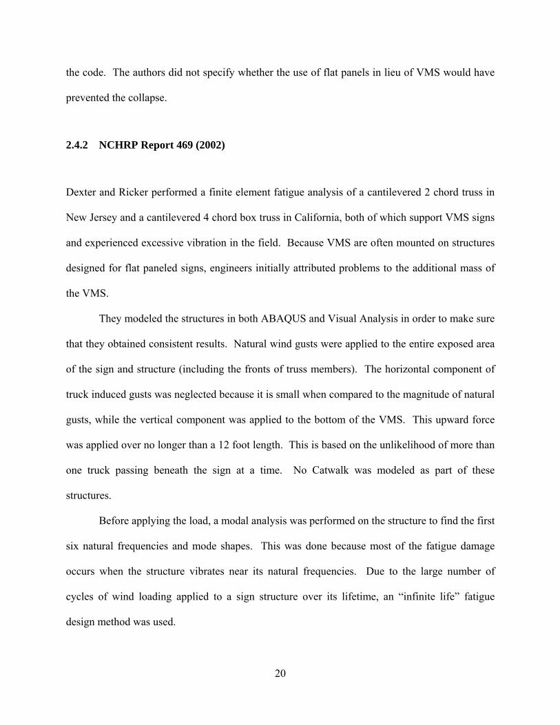
the code. The authors did not specify whether the use of flat panels in lieu of VMS would have

prevented the collapse.

2.4.2 NCHRP Report 469 (2002)

Dexter and Ricker performed a finite element fatigue analysis of a cantilevered 2 chord truss in

New Jersey and a cantilevered 4 chord box truss in California, both of which support VMS signs

and experienced excessive vibration in the field. Because VMS are often mounted on structures

designed for flat paneled signs, engineers initially attributed problems to the additional mass of

the VMS.

They modeled the structures in both ABAQUS and Visual Analysis in order to make sure

that they obtained consistent results. Natural wind gusts were applied to the entire exposed area

of the sign and structure (including the fronts of truss members). The horizontal component of

truck induced gusts was neglected because it is small when compared to the magnitude of natural

gusts, while the vertical component was applied to the bottom of the VMS. This upward force

was applied over no longer than a 12 foot length. This is based on the unlikelihood of more than

one truck passing beneath the sign at a time. No Catwalk was modeled as part of these

structures.

Before applying the load, a modal analysis was performed on the structure to find the first

six natural frequencies and mode shapes. This was done because most of the fatigue damage

occurs when the structure vibrates near its natural frequencies. Due to the large number of

cycles of wind loading applied to a sign structure over its lifetime, an “infinite life” fatigue

design method was used.

20

The researchers found that the extra VMS mass would decrease the natural frequency of

the structure and would typically be countered by an increase in stiffness in order to control dead

load deflection. They believe that it is instead the soffit area on the underside of the sign that

causes the vibration problems.

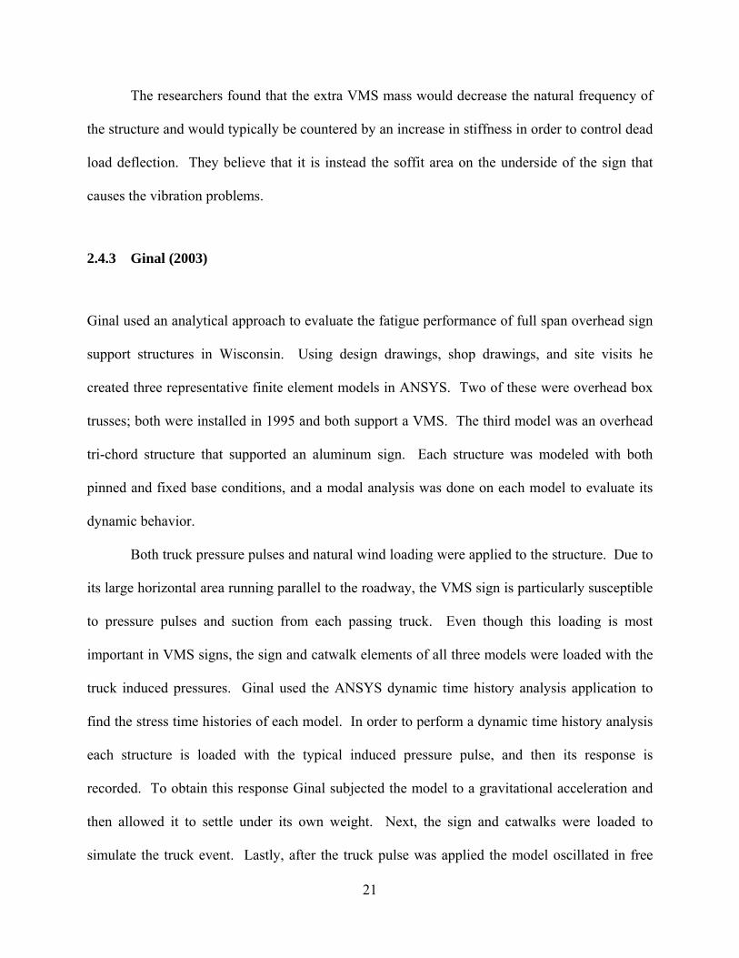
2.4.3 Ginal (2003)

Ginal used an analytical approach to evaluate the fatigue performance of full span overhead sign

support structures in Wisconsin. Using design drawings, shop drawings, and site visits he

created three representative finite element models in ANSYS. Two of these were overhead box

trusses; both were installed in 1995 and both support a VMS. The third model was an overhead

tri-chord structure that supported an aluminum sign. Each structure was modeled with both

pinned and fixed base conditions, and a modal analysis was done on each model to evaluate its

dynamic behavior.

Both truck pressure pulses and natural wind loading were applied to the structure. Due to

its large horizontal area running parallel to the roadway, the VMS sign is particularly susceptible

to pressure pulses and suction from each passing truck. Even though this loading is most

important in VMS signs, the sign and catwalk elements of all three models were loaded with the

truck induced pressures. Ginal used the ANSYS dynamic time history analysis application to

find the stress time histories of each model. In order to perform a dynamic time history analysis

each structure is loaded with the typical induced pressure pulse, and then its response is

recorded. To obtain this response Ginal subjected the model to a gravitational acceleration and

then allowed it to settle under its own weight. Next, the sign and catwalks were loaded to

simulate the truck event. Lastly, after the truck pulse was applied the model oscillated in free

21

vibration and the response was recorded for five seconds. Stress ranges could then be

established from these stress histories.

The method proposed by Ginal to account for fatigue is a two step process:

1. Accurately account for loading scenarios of the structure and record a

comprehensive response to these loadings.

2. Use a fatigue analysis procedure to determine fatigue life.

The stress life method, as recommended by AASHTO (2004), was used in this procedure.

Fatigue life due to both truck induced pulses and natural wind were determined separately.

Determining the fatigue life from the truck pulses involved the previously described analysis of

the structure’s response to loadings, quantifying the probability of this loading, and finding the

damage accumulation over a period of time. To find the fatigue life due to natural wind Ginal

collected the wind speed and direction data from the National Climatic Data Center (NCDC)

(http://cdo.ncdc.noaa.gov), used a rainflow counting algorithm to transform stress histories into

stress ranges, and then used the Palmgren-Miner rule (Bannantine 1990) to assess yearly fatigue

damage. Table 2-2 summarizes the fatigue life predicted for the critical members in the three

structures under investigation.

Table 2-2 Expected fatigue life from Ginal (2003)

Confidence Level Overhead tri-chord truss with flat signs

Overhead box truss with VMS -1

Overhead box truss with VMS - 2

95% 3.8 years 12.0 years 6.5 years 70% 5.3 years 17.0 years 9.2 years 50% 6.5 years 20.7 years 11.2 years 20% 8.5 years 27.0 years 14.7 years

The 95% confidence levels estimates were obtained using the AASHTO S-N curves for

the critical fatigue detail of the sign structure. Typically, sign structures are designed with a

22

minimum service life of 25 years so these very low results led Ginal to question the accuracy of

the AASHTO curves because he felt that his method was done correctly.

2.4.4 Li (2005)

Li modeled a cantilevered double mast arm, a cantilevered single mast arm, a box truss, a

monotube, and a tri-chord sign structure based on design drawings of such structures located in

Indiana, focusing particularly on the modeling of critical connections in these structures. Each of

these structures supported typical aluminum highway signs. Similar to Ginal (2003), Li modeled

these structures using ANSYS.

After acknowledging the four different potential types of wind loads, galloping, vortex

shedding, natural wind, and truck induced wind, Li assumed that the natural wind gust loading

causes fatigue damage in sign structures. Galloping has rarely been observed in the field except

for single mast arms; only structures with large dimensions are subjected to vortex shedding, and

truck induced gusts are more critical in structures with large areas parallel to the ground. As

such, all loads other than natural wind were ignored. In order to perform a dynamic finite

element analysis to obtain a stress time history, a natural wind induced force time history is

generally necessary. The Weibull distribution (Stevens and Smulders 1979) was used to

represent these wind speed distributions and the wind was assumed to blow perpendicular to the

sign’s plane.

Similarly to the Ginal thesis, the fatigue analytical method included the use of SN curves,

Miner’s rule, rainflow counting, and fatigue limits. Before using these tools, transient dynamic

analyses were performed on the finite element models to obtain stress-time histories at critical

23

details. Using wind data from the NCDC for different cities in Indiana, the computed fatigue

lives were found to vary at different sites.

Li found the fatigue lives of the different structural connection details for each of his

models except for the single mast arm cantilever. This was excluded because the research

focused only on fatigue induced by natural wind and fatigue in the single mast arm structure is

thought to be caused by galloping. Unlike the S-N curve method used in Ginal (2003), Li used a

variable amplitude fatigue limit (VAFL) method. This method identifies the level below which

damage will not occur for variable amplitude loading spectrums and is considered to be less

conservative then the S-N method. Li found that practically all connections in the box truss,

cantilevered monotube, and tri-chord truss have an infinite lifetime. Of those connections that

did not, the shortest expected fatigue life is 123 years. The connections in the double mast arm

cantilever had lifetimes ranging from 32 years to infinity.

These expected lifetimes are drastically different from those found in Ginal. Li qualified

these lifetimes by acknowledging that imperfections in connections may be found in the field

which would lead to shorter life expectancies. Also, the modeled signs were designed based on

the 2001 AASHTO sign support specifications which are believed to be conservative.

2.4.5 Park and Stallings (2006)

Park and Stallings sought to perform a fatigue evaluation of an overhead box truss and to

investigate the applicability of the AASHTO 2001 sign support specifications to non-

cantilevered structures. Rather than using a finite element model to aid in the prediction of

fatigue life, the researchers performed in field monitoring tests. Strain gages and a wind

anemometer were attached on two box trusses supporting VMS signs. The anemometer

24

measured the velocity and direction of the wind. Two structures were monitored for 31 and 82

days, respectively. This difference in monitoring times was not explained.

During the monitoring period, a rain flow cycle counting algorithm (ASTM 1049E) was

performed in order to record the number and magnitude of only the significant strain cycles. The

response associated with both natural and truck induced gusts was measured, but it was found

that natural wind caused most of the significant cycles. The number of strain cycles measured

over the monitoring period was then extrapolated into the number that would occur in one year

and the fatigue lives of each monitored truss member was calculated using the procedure defined

in the AASHTO 2004 bridge specifications. The majority of the members in the structure

monitored for 31 days have an infinite life, but one diagonal has a life of 28 years. All of the

members in the second structure have an infinite life.

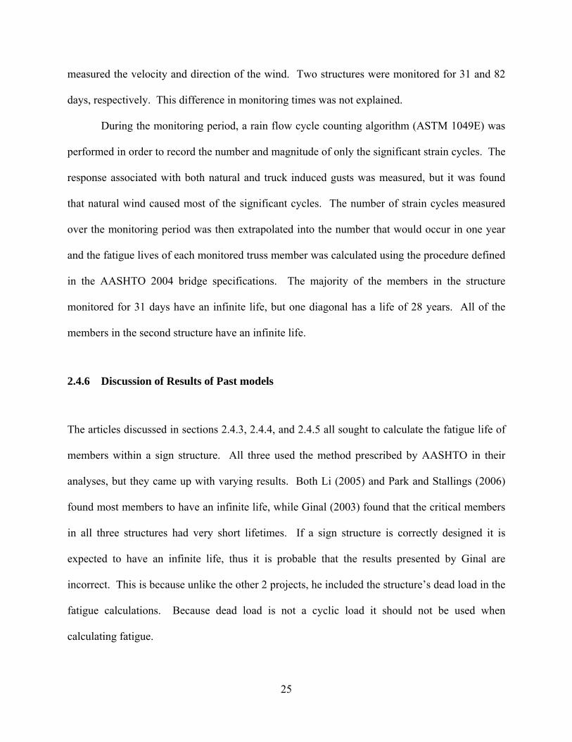
2.4.6 Discussion of Results of Past models

The articles discussed in sections 2.4.3, 2.4.4, and 2.4.5 all sought to calculate the fatigue life of

members within a sign structure. All three used the method prescribed by AASHTO in their

analyses, but they came up with varying results. Both Li (2005) and Park and Stallings (2006)

found most members to have an infinite life, while Ginal (2003) found that the critical members

in all three structures had very short lifetimes. If a sign structure is correctly designed it is

expected to have an infinite life, thus it is probable that the results presented by Ginal are

incorrect. This is because unlike the other 2 projects, he included the structure’s dead load in the

fatigue calculations. Because dead load is not a cyclic load it should not be used when

calculating fatigue.

25

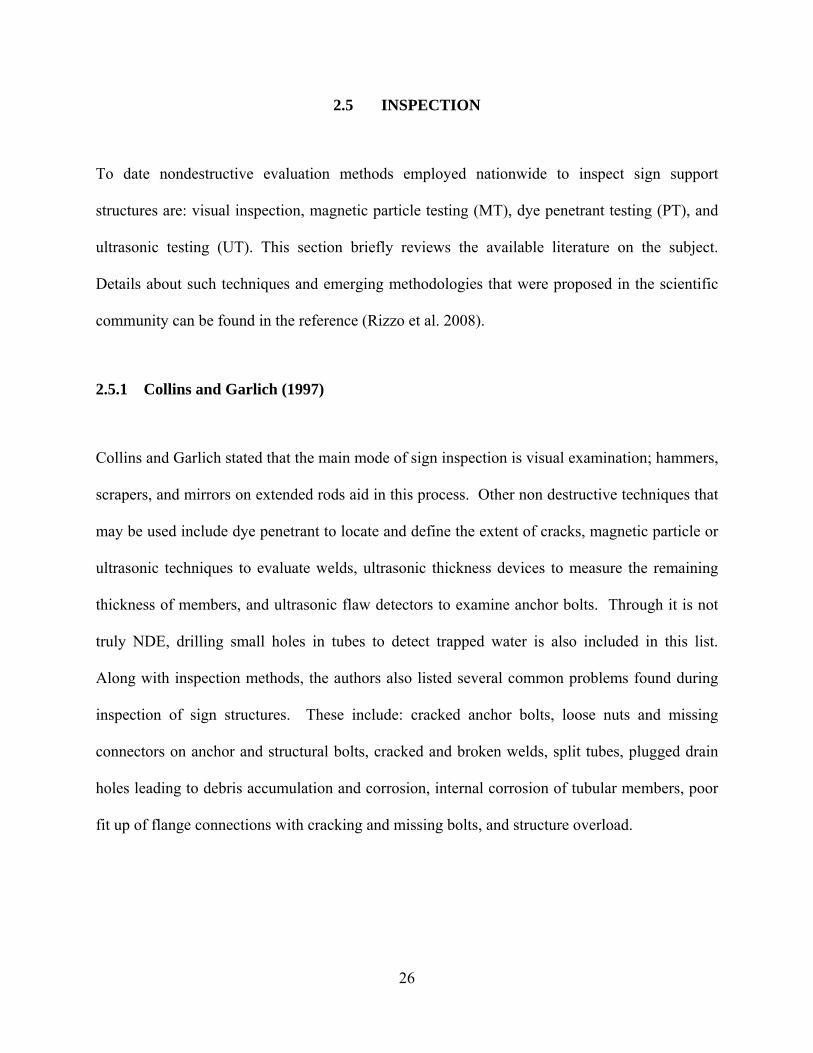
2.5 INSPECTION

To date nondestructive evaluation methods employed nationwide to inspect sign support

structures are: visual inspection, magnetic particle testing (MT), dye penetrant testing (PT), and

ultrasonic testing (UT). This section briefly reviews the available literature on the subject.

Details about such techniques and emerging methodologies that were proposed in the scientific

community can be found in the reference (Rizzo et al. 2008).

2.5.1 Collins and Garlich (1997)

Collins and Garlich stated that the main mode of sign inspection is visual examination; hammers,

scrapers, and mirrors on extended rods aid in this process. Other non destructive techniques that

may be used include dye penetrant to locate and define the extent of cracks, magnetic particle or

ultrasonic techniques to evaluate welds, ultrasonic thickness devices to measure the remaining

thickness of members, and ultrasonic flaw detectors to examine anchor bolts. Through it is not

truly NDE, drilling small holes in tubes to detect trapped water is also included in this list.

Along with inspection methods, the authors also listed several common problems found during

inspection of sign structures. These include: cracked anchor bolts, loose nuts and missing

connectors on anchor and structural bolts, cracked and broken welds, split tubes, plugged drain

holes leading to debris accumulation and corrosion, internal corrosion of tubular members, poor

fit up of flange connections with cracking and missing bolts, and structure overload.

26

2.5.2 NCHRP Report 469 (2002)

In their report Dexter and Ricker focused on failures of cantilever sign structures. The results of

a survey sent to all DOTs indicate that common areas showing fatigue cracking or vibration are

the column-to-base welded connection, truss tube to tube welded connections, and the mast arm

connection. The survey also found multiple occurrences of loose or missing anchor rods.

Sign structures were divided into Class A and Class B structures; Class A being those

that are more susceptible to wind-induced fatigue damage. NCHRP Report 469 states that Class

A structures should be inspected at least every 4 years, while Class B should be inspected at least

every 8 years. The authors cite visual inspection as the main way to inspect cracks. This

inspection should consist of close up or hands on view of the base of the post and the mast arm

or truss to post connection. The rest of the structure may be inspected from the ground, however

if evidence of cracks is noted they must be inspected more closely. Some NDE methods are also

suggested for inspection. Like Collins and Garlich (1997), this report recommended magnetic

particles or liquid penetrant as a means to detect cracks, but adds that these should only be used

when a sound reason to suspect cracking exists. Ultrasonic testing can also be used for crack

detection. This report suggested that when an inspector notices a fatigue crack in the connection

on one structure it is likely too late to repair that structure, but it may be practical to apply

ultrasonic testing to similar connections in the same area in hopes of catching other cracks at a

stage where they may be remediated.

27

2.5.3 Li (2005)

Li names five different types of highway sign structures: the double mast arm cantilever, the

single mast arm cantilever, the box truss, the monotube structure, and the trichord sign structure

(where the last three are full span structures). The primary mode of inspection of these signs for

cracks is visual inspection, which can be done on its own or in combination with other NDE

methods. Visual inspection is preferred because it is not too expensive, but it does have the

limitation of human error. PT, MT, or UT can be done to supplement the visual inspections

findings. PT is inexpensive and can reliably find cracks on smooth surfaces. MT can detect

defects on and just below the surface, but its accuracy is not great when testing welded material.

UT can also detect surface and subsurface cracks. Unlike PT and MT, UT requires a high level

of inspector training thus making it more expensive.

28

3.0 FINITE ELEMENT MODEL OF A 4 CHORD TRUSS

This chapter focuses on the development of a computer model for a highway sign structure

located in the jurisdiction of the Pennsylvania Department of Transportation (PennDOT). After

describing the structure examined in this research there will be a brief review of the finite

element method and then the model will be discussed in detail.

3.1 THE STRUCTURE

No field research is included in this study, instead a real structure was modeled to obtain results.

A survey conducted in the spring of 2008 by the University of Pittsburgh found that PennDOT

uses several types of sign structures including overhead trusses, cantilevered poles and

monotubes (Rizzo et al. 2008). One overhead truss that is widely used is the four chord box

truss. In this study an overhead box truss structure located on Interstate 279 in Allegheny County

within the jurisdiction of PennDOT District 11 is taken into consideration. Though the truss in

many sign structures is made of tubular members, this particular truss is made of angles. This is

important to note because the use of angles allows for bolted connections between members.

The type of connection affects fatigue life and this aspect will be discussed in depth in chapter 5.

The I-279 structure spans nine lanes of traffic including four in the north (outbound)

direction, two in the High Occupancy Vehicle (HOV) lane, and three in the south (inbound)

29

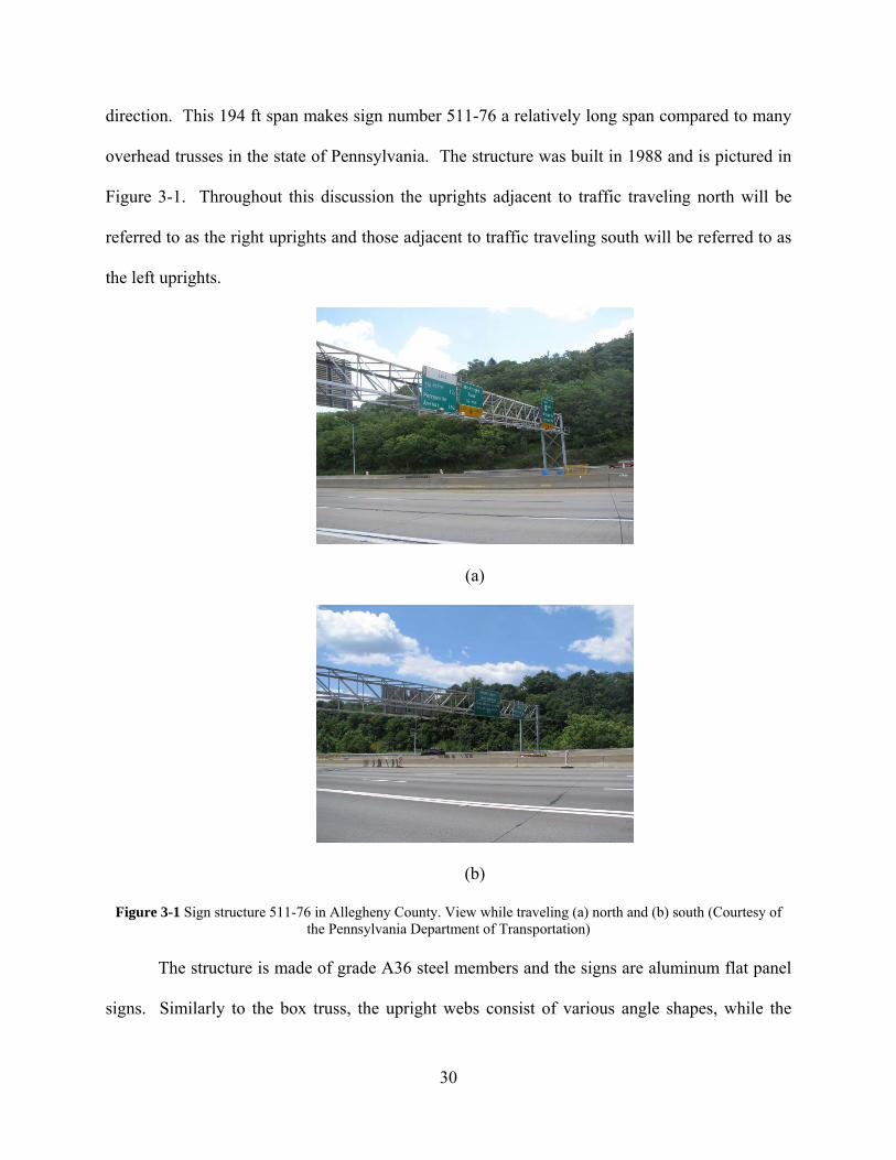
direction. This 194 ft span makes sign number 511-76 a relatively long span compared to many

overhead trusses in the state of Pennsylvania. The structure was built in 1988 and is pictured in

Figure 3-1. Throughout this discussion the uprights adjacent to traffic traveling north will be

referred to as the right uprights and those adjacent to traffic traveling south will be referred to as

the left uprights.

(a)

(b)

Figure 3-1 Sign structure 511-76 in Allegheny County. View while traveling (a) north and (b) south (Courtesy of the Pennsylvania Department of Transportation)

The structure is made of grade A36 steel members and the signs are aluminum flat panel

signs. Similarly to the box truss, the upright webs consist of various angle shapes, while the

30

uprights are wide flange shapes. The specific sizes and material properties of all members can

be found in Appendix A.

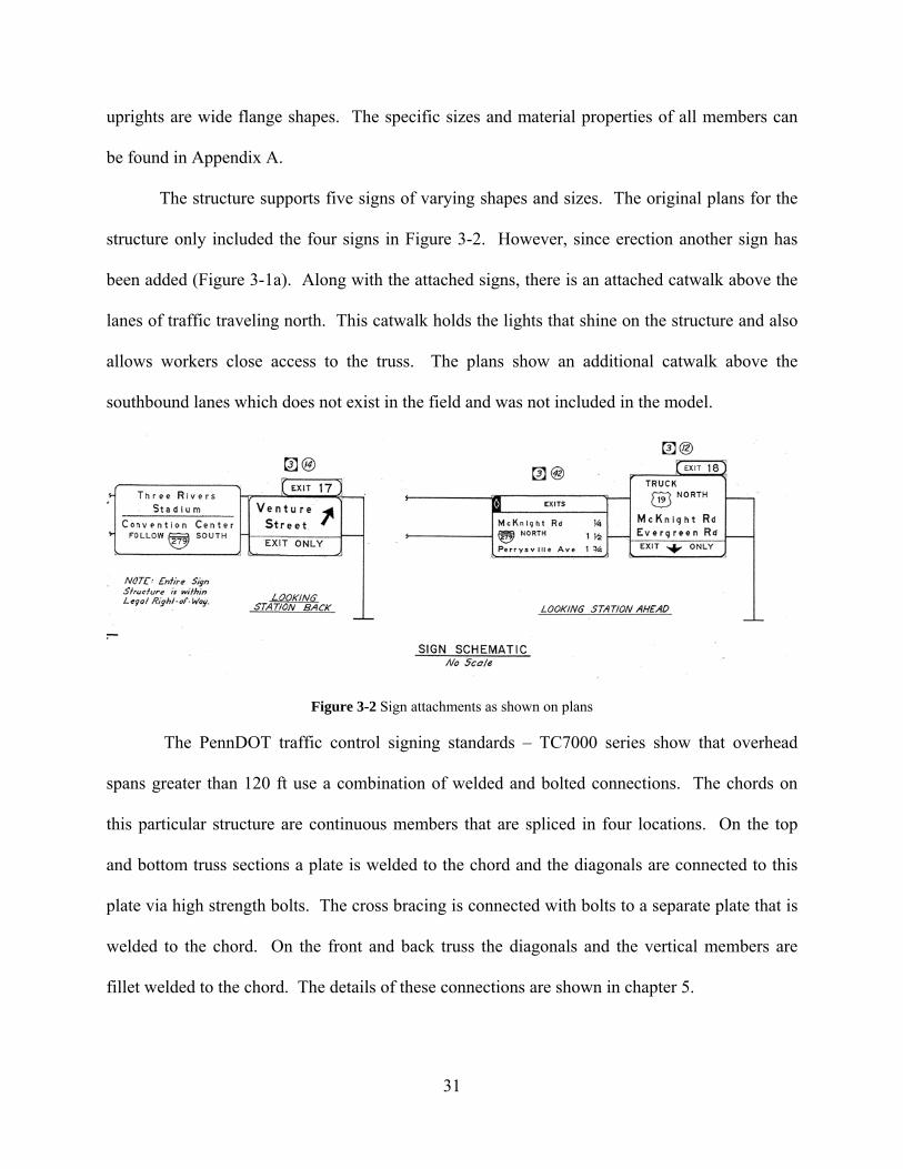
The structure supports five signs of varying shapes and sizes. The original plans for the

structure only included the four signs in Figure 3-2. However, since erection another sign has

been added (Figure 3-1a). Along with the attached signs, there is an attached catwalk above the

lanes of traffic traveling north. This catwalk holds the lights that shine on the structure and also

allows workers close access to the truss. The plans show an additional catwalk above the

southbound lanes which does not exist in the field and was not included in the model.

Figure 3-2 Sign attachments as shown on plans

The PennDOT traffic control signing standards – TC7000 series show that overhead

spans greater than 120 ft use a combination of welded and bolted connections. The chords on

this particular structure are continuous members that are spliced in four locations. On the top

and bottom truss sections a plate is welded to the chord and the diagonals are connected to this

plate via high strength bolts. The cross bracing is connected with bolts to a separate plate that is

welded to the chord. On the front and back truss the diagonals and the vertical members are

fillet welded to the chord. The details of these connections are shown in chapter 5.

31

3.2 THE FINITE ELEMENT METHOD

Structural analysis typically uses the finite element method because as complications arise (e.g.

geometric, boundary conditions, physical phenomena, etc.) analytical solutions become

intractable. In the traditional finite element method for structural analysis the geometry is

divided into a series of discrete small segments (i.e. finite elements), and the displacement is

interpolated within each segment using simple polynomial functions. Therefore, the governing

differential equations for the structural response are transformed into a linear system of

equations, which can be solved computationally to obtain an approximation to the displacement

field. The resulting displacement field can then be further processed to obtain estimates to the

pointwise stresses and strains throughout the structure (Logan 2002).

3.3 BUILDING THE MODEL

In this study the commercial finite element analysis software ANSYS version 11.0 was chosen

for the analysis of the structural response of the chosen sign structure. The use of this software

allowed for a comparison of the results obtained in this study with the results published in Ginal

(2003) and Li (2005) because they also used ANSYS.

3.3.1 Steps for Modeling

Several solid mechanics models were built in order to run a quasi-static analysis with a wind load

applied as a traction force to the signs and super structure. The structures considered were

32

assumed to behave linear elastically, with small strains and displacements due to the applied

wind loading. As such, the discretized system of equations for the finite element analysis can be

given as:

[m] { }+ [c]{ }+[k]{x} = {F(t)} (3.1)

Where [m] is the mass matrix, { } is an acceleration vector, [c] is the viscous damping

coefficient matrix, { } is the velocity vector, [k] is the stiffness matrix, {x} is the displacement

vector, and F(t) is the force on the structure. Because the results of this model were used to

perform a fatigue analysis, the structure’s self weight was not included in the analysis. Damping

was also not included, thus the equation of motion becomes:

[k]{x} = {F(t)} (3.1)

The steps required to build a finite element model for a structure are as follows

1. Define nodes and build lines

2. Select element types

3. Define section properties

4. Define material properties

5. Select an appropriate mesh size and mesh elements

Step 1 was accomplished using the structure’s general plan and elevation design drawing

provided by PennDOT. This plan is shown in Appendix A. The basic geometry of the sign

structure and the signs themselves were input into the model using the ANSYS Parametric

Design Language (APDL) (ANSYS 2007). The model shown in Figure 3-3a and 3-3b represent

the structure with 4 and 5 signs, respectively.

33

(a)

(b)

Figure 3-3 ANSYS model of sign structure 511-76. (a) Model with 4 aluminum signs attached. (b) Model with 5 aluminum signs attached.

Finite elements that could efficiently provide accurate estimates to the response of the

actual structural members needed to be chosen in order to perform step 2. As previously noted,

the main component of the structure is a steel box truss. The steel components were modeled

34

using a three dimensional 2 node beam element and the aluminum signs and the catwalk were

modeled using a three dimensional 4 node shell element (ANSYS 2007).

The section properties and material properties for each element are specific to the

structural shape and material being used. Section properties input into this model were cross

sectional area, moment of inertia, and member thickness. The material properties for the linear

elastic model include Young’s modulus, Poison’s ratio, and material density. Typical properties

of steel and aluminum were used (Mamlouk and Zaniewski 1999). A table of the section

properties used for each member is included in Appendix A.

The nonlinearity in connections between members and at the base was assumed to be

negligible for the purposes of this work, and therefore, foundations and anchor rods were not

explicitly considered in the models. A mode shape analysis was performed on the structure

considering both a fixed and pinned base condition. Table 3-1 compares the natural frequencies

found in the two cases for the first ten modes, and Figure 3-4 and 3-5 show the first four mode

shapes for the pinned case and fixed case respectively. Table 3-1 shows that from mode 4 and

up, the base fixity does not have much impact on the natural frequency of the structure. The

variation in modes 1-3 can be explained by examining Figures 3-4 and 3-5. When the

corresponding truss movements in the Figures are matched, it can be seen that mode 1 from

Figure 3-4 and mode 3 from figure 3-5 are both a lateral movement of the truss. This is the only

mode shape that is affected by the base conditions. In order to excite this mode, a wind along the

length of the truss would need to be applied. Since this situation was not considered in the

analysis, the base fixity will not have a large effect on the stresses developed in the model. As

such, the bottom of the support was modeled as fixed so as not to allow rotation or translation in

any direction.

35

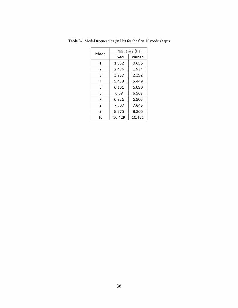
Table 3-1 Modal frequencies (in Hz) for the first 10 mode shapes

Mode Frequency (Hz) Fixed  Pinned 

1  1.952  0.656 2  2.436  1.934 3  3.257  2.392 4  5.453  5.449 5  6.101  6.090 6  6.58  6.563 7  6.926  6.903 8  7.707  7.646 9  8.375  8.366 10  10.429  10.421 

36

Figure 3-4 First four mode shapes in the pinned base case.

37

Figure 3-5 First four mode shapes in the fixed base case

The signs on the structure are attached to the truss via vertical W sections as shown in

Figure 3-6. More detailed schematics of this connection are shown in Appendix A. The sign

mesh was defined in such a way that the nodes on the vertical beam lined up with those on the

sign. These coincident nodes were then merged in order to connect the sign to the beam.

38

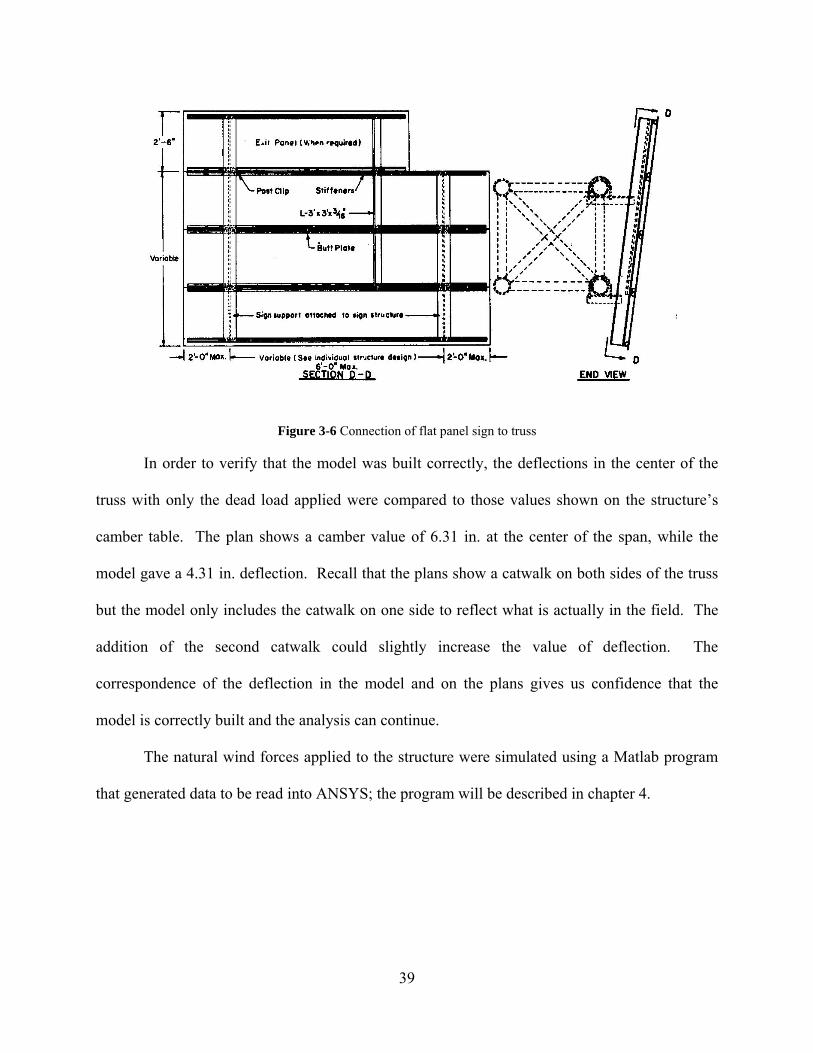
Figure 3-6 Connection of flat panel sign to truss

In order to verify that the model was built correctly, the deflections in the center of the

truss with only the dead load applied were compared to those values shown on the structure’s

camber table. The plan shows a camber value of 6.31 in. at the center of the span, while the

model gave a 4.31 in. deflection. Recall that the plans show a catwalk on both sides of the truss

but the model only includes the catwalk on one side to reflect what is actually in the field. The

addition of the second catwalk could slightly increase the value of deflection. The

correspondence of the deflection in the model and on the plans gives us confidence that the

model is correctly built and the analysis can continue.

The natural wind forces applied to the structure were simulated using a Matlab program

that generated data to be read into ANSYS; the program will be described in chapter 4.

39

4.0 WIND LOADING ON SIGN STRUCTURES

In order to obtain accurate results from the finite element model the load placed on it must be

representative of the actual loading scenario. Other than self-weight, most loads applied to

highway signs structures are dynamic in nature. These include but are not limited to wind gusts,

ground motion, and vehicle impact. Dynamic wind loads are the focus of this chapter because

every sign structure is subjected to them regardless of location. Wind induced damage on

highway sign structures can occur due to galloping, vortex shedding, truck induced gusts, or

natural wind loading. The severity of the damage inflicted upon a structure varies based on

which of these phenomena occurs and in some cases is dependent on the sign structure

configuration (i.e. whether it is cantilevered or not). Though all four phenomena are described

herein, this chapter will mainly focus on the effects of natural wind on sign structures and the

development of the wind loading that is applied to the ANSYS structural model.

4.1 DYNAMIC WIND LOADS

The American Association of State Highway and Transportation Officials (AASHTO) lists four

types of wind fatigue design loads in the 2001 Standard Specifications for Structural Supports for

Highway Signs, Luminaries and Traffic Signals: galloping, vortex shedding, natural wind gusts,

and truck induced gusts. These four are included in order to “avoid large-amplitude vibrations

40

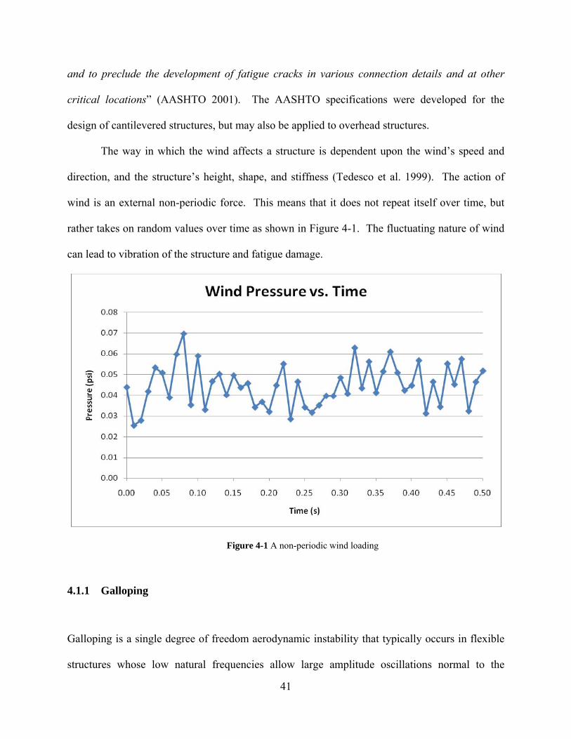
and to preclude the development of fatigue cracks in various connection details and at other

critical locations” (AASHTO 2001). The AASHTO specifications were developed for the

design of cantilevered structures, but may also be applied to overhead structures.

The way in which the wind affects a structure is dependent upon the wind’s speed and

direction, and the structure’s height, shape, and stiffness (Tedesco et al. 1999). The action of

wind is an external non-periodic force. This means that it does not repeat itself over time, but

rather takes on random values over time as shown in Figure 4-1. The fluctuating nature of wind

can lead to vibration of the structure and fatigue damage.

Figure 4-1 A non-periodic wind loading

4.1.1 Galloping

Galloping is a single degree of freedom aerodynamic instability that typically occurs in flexible

structures whose low natural frequencies allow large amplitude oscillations normal to the

41

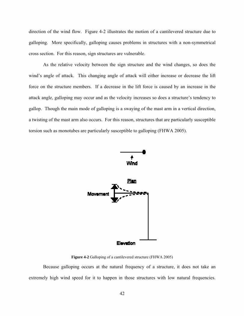
direction of the wind flow. Figure 4-2 illustrates the motion of a cantilevered structure due to

galloping. More specifically, galloping causes problems in structures with a non-symmetrical

cross section. For this reason, sign structures are vulnerable.

As the relative velocity between the sign structure and the wind changes, so does the

wind’s angle of attack. This changing angle of attack will either increase or decrease the lift

force on the structure members. If a decrease in the lift force is caused by an increase in the

attack angle, galloping may occur and as the velocity increases so does a structure’s tendency to

gallop. Though the main mode of galloping is a swaying of the mast arm in a vertical direction,

a twisting of the mast arm also occurs. For this reason, structures that are particularly susceptible

torsion such as monotubes are particularly susceptible to galloping (FHWA 2005).

Figure 4-2 Galloping of a cantilevered structure (FHWA 2005)

Because galloping occurs at the natural frequency of a structure, it does not take an

extremely high wind speed for it to happen in those structures with low natural frequencies.

42

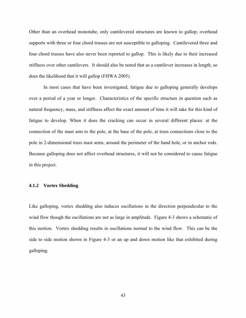
Other than an overhead monotube, only cantilevered structures are known to gallop; overhead

supports with three or four chord trusses are not susceptible to galloping. Cantilevered three and

four chord trusses have also never been reported to gallop. This is likely due to their increased

stiffness over other cantilevers. It should also be noted that as a cantilever increases in length, so

does the likelihood that it will gallop (FHWA 2005).

In most cases that have been investigated, fatigue due to galloping generally develops

over a period of a year or longer. Characteristics of the specific structure in question such as

natural frequency, mass, and stiffness affect the exact amount of time it will take for this kind of

fatigue to develop. When it does the cracking can occur in several different places: at the

connection of the mast arm to the pole, at the base of the pole, at truss connections close to the

pole in 2-dimensional truss mast arms, around the perimeter of the hand hole, or in anchor rods.

Because galloping does not affect overhead structures, it will not be considered to cause fatigue

in this project.

4.1.2 Vortex Shedding

Like galloping, vortex shedding also induces oscillations in the direction perpendicular to the

wind flow though the oscillations are not as large in amplitude. Figure 4-3 shows a schematic of

this motion. Vortex shedding results in oscillations normal to the wind flow. This can be the

side to side motion shown in Figure 4-3 or an up and down motion like that exhibited during

galloping.

43

Figure 4-3 Vortex Shedding (FHWA 2005)

The members that make up a sign structure can be referred to as bluff bodies; this means

that they are not streamlined to cut through the wind. The flow of wind around a bluff body is

shown in Figure 4-4. As the wind tries to make its way around the section, it separates away

from it on the back end creating a high shear region. The curled up lines in the figure represent

shear and if they begin to alternate the side on which they curl up, movement will be induced

(Holmes 2007).

Typically, vortex shedding occurs in circular cylinders but it can occur in other bluff

bodies such as triangles, rectangles, or H and L shapes. Similar to galloping, vibration due to

vortex shedding occurs when the wind speed allows the frequency of the shedding to become

about equal to the structure’s natural frequency. The structure only shows excessive vibration

when the wind velocity causes this resonant condition (Liu 1991). A constant wind speed

between 10 and 45 mph is necessary to predicate vortex shedding; if there is turbulence it will

44

disturb the formation of vortices. Speeds less than 10 mph will not induce vibration while

speeds greater than 45 mph are too turbulent for vortices to be shed (AASHTO 2001). The

FHWA says that winds between 10 and 35 mph are most likely to cause vortex shedding (FHWA

2005), while the AASHTO 2001 sign structure specifications set the upper limit at 45 mph

(AASHTO 2001). If resonance is reached and the wind flow is not turbulent, higher wind speeds

may cause vortex shedding. Vortices can be shed at wind speeds less than 10 mph, though they

will not impart sufficient energy to excite most structures (AASHTO 2001).

The AASHTO sign support specifications recommend that a sign or sign blank is

attached prior to erection and does not require a sign structure to be designed to resist vortex

shedding. Blank signs are recommended because they can break up the wind vortices by causing

local turbulence. Because vortex shedding does not affect overhead structures, it will not be

considered to cause fatigue in this project.

Figure 4-4 Shedding of vortices on a bluff body

4.1.3 Truck Induced Gusts

As large trucks pass under sign structures they produce dynamic wind pressures in both a

direction perpendicular to the sign face and an upward direction. The horizontal gust created by

45

a truck is much smaller than that created by natural wind, so much so that it is negligible. The

magnitude of the vertical pressure varies with truck speed, height of the sign, and sign geometry.

For example, the magnitude of the gust is directly proportional to the speed of the truck. Also,

the higher the sign is above the roadway, the lower the magnitude of the gust. In fact, it is

widely accepted that truck gusts go to zero at a height of about 33 ft above the roadway.

VMS signs are particularly susceptible to fatigue damage caused by truck induced gusts because

unlike flat aluminum signs they have a large area parallel to the road on which an upward force

can act. An older VMS sign can be up to four feet deep making truck induced gusts a significant

cause of fatigue in its supporting structures. Typically, fatigue cracking due to truck induced

gusts takes several years to develop. When it does, cracks might occur in the following places:

the connection to the mast arm to the pole, at truss connections, at the base of the pole to the

weld joining the pole to the base, at hand holes, or in anchor rods. Because the sign structure in

this project supports a flat panel aluminum sign, the affects of truck gusts on the model were not

included.

4.2 BASIC CHARACTERISTICS OF NATURAL WIND

The previous section presented the basics of three of the wind phenomena that could act

on highway sign structures. This current section will present the way in which natural wind

works and acts on sign structures. The nature of wind speed is that it fluctuates as shown in

Figure 4-1.

The wind time history v(t) is the changing value of wind speed with respect to time.

When applied to a sign structure we can consider two components: a mean component v and a

46

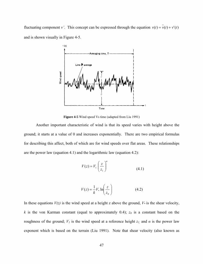
fluctuating component v’. This concept can be expressed through the equation )(')()( tvtvtv +=

and is shown visually in Figure 4-5.

Figure 4-5 Wind speed Vs time (adapted from Liu 1991)

Another important characteristic of wind is that its speed varies with height above the

ground; it starts at a value of 0 and increases exponentially. There are two empirical formulas

for describing this affect, both of which are for wind speeds over flat areas. These relationships

are the power law (equation 4.1) and the logarithmic law (equation 4.2):

α

⎟⎟⎠

⎞⎜⎜⎝

⎛=

11)(

zzVzV (4.1)

⎟⎟⎠

⎞⎜⎜⎝

⎛=

0* ln1)(

zzV

kzV (4.2)

In these equations V(z) is the wind speed at a height z above the ground, V* is the shear velocity,

k is the von Karman constant (equal to approximately 0.4); z0 is a constant based on the

roughness of the ground; V1 is the wind speed at a reference height z1, and α is the power law

exponent which is based on the terrain (Liu 1991). Note that shear velocity (also known as

47

friction velocity) V* is not a physical velocity, but rather a way of writing shear stress in units of

velocity (Holmes 2007). The logarithmic law was originally derived for the turbulent boundary

layer on a flat plate while the power law has no theoretical basis (Holmes 2007). Because the

logarithmic law is more difficult to use and sometimes produces negative wind speeds when the

height in question is below the base height z0, the power law is generally used in engineering

applications. As shown by Figure 4-6 the two laws produce very similar results.

Figure 4-6 Comparison of Logarithmic and Power law (adapted from Holmes 2007)

v/v10

The logarithmic law takes into account the effect of the surface roughness on the wind

speed. The ground exerts a retarding force known as surface drag on wind as it flows. The

amount of surface drag depends on the type of terrain. For example, there are measured values

of surface drag for very flat terrain, open terrain, suburban terrain, and dense urban terrain.

Surface drag tends to increase as the terrain becomes denser because the wind flow is easily

broken up due to the many different obstacles around which the wind must flow. Flat open

terrain has a very low surface drag coefficient because the wind is not subjected to any obstacles.

48

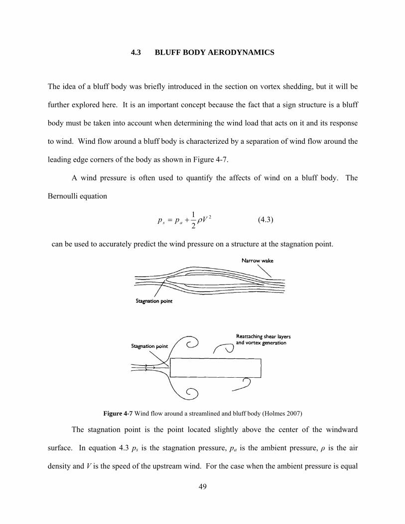
4.3 BLUFF BODY AERODYNAMICS

The idea of a bluff body was briefly introduced in the section on vortex shedding, but it will be

further explored here. It is an important concept because the fact that a sign structure is a bluff

body must be taken into account when determining the wind load that acts on it and its response

to wind. Wind flow around a bluff body is characterized by a separation of wind flow around the

leading edge corners of the body as shown in Figure 4-7.

A wind pressure is often used to quantify the affects of wind on a bluff body. The

Bernoulli equation

2

21 Vpp as ρ+= (4.3)

can be used to accurately predict the wind pressure on a structure at the stagnation point.

Figure 4-7 Wind flow around a streamlined and bluff body (Holmes 2007)

The stagnation point is the point located slightly above the center of the windward

surface. In equation 4.3 ps is the stagnation pressure, pa is the ambient pressure, ρ is the air

density and V is the speed of the upstream wind. For the case when the ambient pressure is equal

49

to the atmospheric pressure, pa = 0. This is the case for the wind acting on the sign structure,

therefore the equation for pressure reduces to equation:

2

21 Vp ρ= (4.4)

4.3.1 Drag

Drag is the resistance caused by an object in a wind flow and increases as the wind flow becomes

more turbulent (Liu 1991). The magnitude of the drag force varies depending on the size and

shape of the object that a wind flow is acting on. For a highway sign structure there will be a

different coefficient of drag (Cd) for the signs and truss members. The actual values used in the

analysis are discussed below.

The sign attachments on the modeled structure are perpendicular to the direction of wind

flow and therefore cause a drag force on the wind. The drag force on a flat panel (such as a sign)

is found by subtracting the leeward pressure from the windward pressure on the panel’s face and

multiplying this number by the total frontal area of the panel. It is estimated that 60% of the drag

is caused by pressure on the front face while the other 40% is caused by pressure on the rear face

(Holmes 2007). The drag coefficient for a square plate in perfectly smooth wind flow is about

1.1, but all of the highway signs on the modeled structure are rectangular so they will have a

slightly larger Cd. The AASHTO sign support specifications give a table of drag coefficient

values in the 2001 specifications (Table 4-1). These values are based on the aspect ratio (sign

length to height) of the sign on which the wind acts. Table 4-2 gives the aspect ratio and the

corresponding value of Cd for the signs in the modeled structure (they are numbered from left to

50

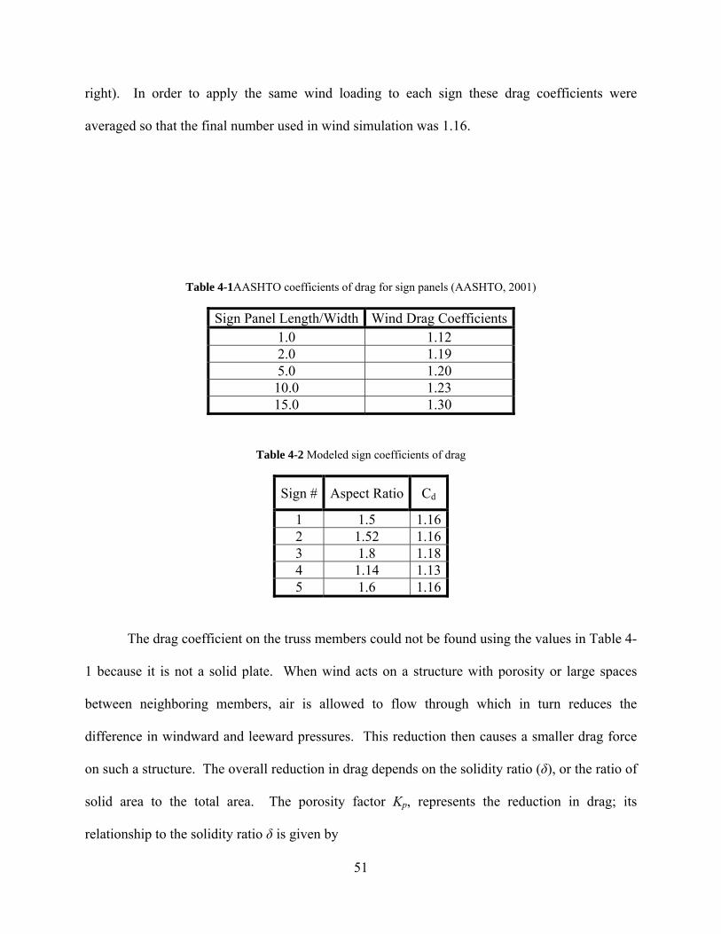
right). In order to apply the same wind loading to each sign these drag coefficients were

averaged so that the final number used in wind simulation was 1.16.

Table 4-1AASHTO coefficients of drag for sign panels (AASHTO, 2001)

Sign Panel Length/Width Wind Drag Coefficients 1.0 1.12 2.0 1.19 5.0 1.20 10.0 1.23 15.0 1.30

Table 4-2 Modeled sign coefficients of drag

Sign # Aspect Ratio Cd

1 1.5 1.162 1.52 1.163 1.8 1.184 1.14 1.135 1.6 1.16

The drag coefficient on the truss members could not be found using the values in Table 4-

1 because it is not a solid plate. When wind acts on a structure with porosity or large spaces

between neighboring members, air is allowed to flow through which in turn reduces the

difference in windward and leeward pressures. This reduction then causes a smaller drag force

on such a structure. The overall reduction in drag depends on the solidity ratio (δ), or the ratio of

solid area to the total area. The porosity factor Kp, represents the reduction in drag; its

relationship to the solidity ratio δ is given by

51

(4.5) 2)1(1 δ−−≅pK

Once the porosity factor is known, the reduced drag coefficient Cdδ, can be found using

the following relationship (Holmes 2007):

(4.6) pdd KCC *=δ

Before the reduced drag coefficient can be found, the drag coefficient for a solid plate with the

dimensions of the truss must be found. The Engineering Sciences Data Unit (EDSU 1970)

provides the drag coefficient of a rectangular plate based its height/breadth ratio h/b:

⎥⎦

⎤⎢⎣

⎡⎟⎠⎞

⎜⎝⎛+⎟

⎠⎞

⎜⎝⎛+=

hb

bhCd *02.010.1 (4.7)

The calculation of the reduced drag coefficient adapted in this study is shown below.

62.15.7

194194

5.7*02.010.1 =⎥⎦

⎤⎢⎣

⎡⎟⎟⎠

⎞⎜⎜⎝

⎛+⎟⎟⎠

⎞⎜⎜⎝

⎛+=

ftft

ftftCd

2393 ftAtruss =

270.05.7*194

==ftft

Atrussδ

467.0)270.01(1 2 =−−=pK

757.0467.0*62.1 ==δdC

Here, Atruss is the area of the truss in this study. The pressure calculated using Cdδ is not

applied to the truss projection Atruss, but rather the gross truss area (194’ x 7.5’).

The drag coefficient for both the signs and the truss members will be used in the following

section to find the pressure load to apply to the model.

52

4.4 WIND SIMULATION

In the field, the wind spectrum is measured by using an anemometer. Then, a

spectrometer connects this signal to a set of filters, and the intensity of those signals that pass

through the filters is measured. Each of these filters has a narrow bandwidth and a different filter

frequency. The value of the spectrum at the filter frequency is found by dividing the measured

signal by the bandwidth of the filter through which it passed. These values are then plotted as a

function of the filter frequency (Liu 1991). A spectrum of wind turbulence is shown in Figure 4-

8.

Figure 4-8 Typical spectrum of wind turbulence S1 or S2 as a function of frequency n (Liu 1991)

Much research has been done in the past in order to develop a spectrum that can

accurately predict the dynamic characteristic of wind. Though we can never predict the

complexity of wind perfectly due to its gusty nature, wind spectra assume that over a time period

the statistical characteristics of wind can be regarded as constant (Davenport 1961a). The

following sections will discuss two such wind spectra: the Davenport spectrum and the Kaimal

spectrum.

53

4.4.1 The Davenport Spectrum

In the early 1960’s A.G. Davenport published a study of 70 spectra of the horizontal component

of gustiness in strong wind. The differences in these spectra were studied by looking at the mean

wind velocity, the ground roughness, and the height above the ground for which they were

produced. The following empirical solution for the wind loading of structures was provided:

dxxkVdffD 3422

1 )1(4*)(

+=

xS (4.8)

where SD is the power spectrum at a height z, f is frequency, k is the drag coefficient depending

on surface roughness, V1 is the wind speed at a standard height of 10 meters (33 feet) , and x

equals 1200f/V1.

The spectra that Davenport analyzed in order to formulate this relationship were mainly

taken in three locations: Sale, Victoria (Australia), Cardington, Bedfordshire (England), and

Cranfield, Bedfordshire (England). A few more measurements were also taken from elsewhere

around the world. The first two places were open grasslands with few trees while the third

location consisted of a rougher terrain. Different anemometer setups were used in each location,

with the most sensitive one being used in Cranfield. The data from all three locations were

normalized into logarithmic spectra. These spectra were very similar at all heights, but they did

show a drop in energy as height increased. This drop off was very small so Davenport assumed

that the spectrum which he was developing was not dependent on height.

Figure 4-8 shows different values found at different locations. The solid curve is a plot

of the empirical relationship given in equation 4-8. Davenport developed this relationship

through trial and error and found it to be a suitable fit for the points in Figure 4-9.

54

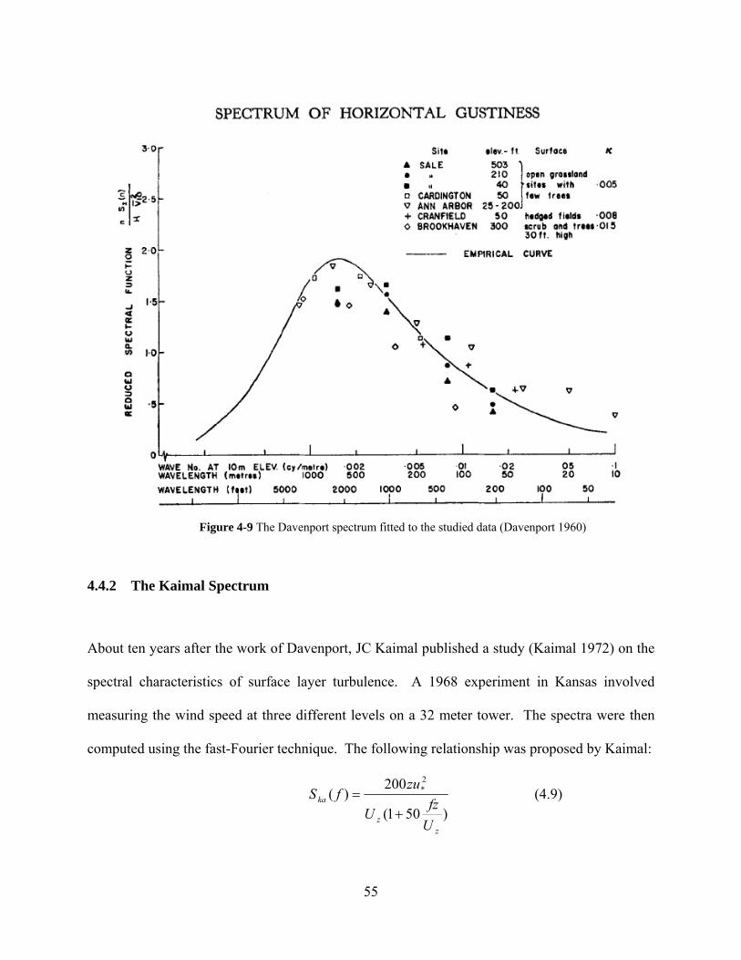
Figure 4-9 The Davenport spectrum fitted to the studied data (Davenport 1960)

4.4.2 The Kaimal Spectrum

About ten years after the work of Davenport, JC Kaimal published a study (Kaimal 1972) on the

spectral characteristics of surface layer turbulence. A 1968 experiment in Kansas involved

measuring the wind speed at three different levels on a 32 meter tower. The spectra were then

computed using the fast-Fourier technique. The following relationship was proposed by Kaimal:

)501(

200)(

2*

zz

ka

UfzU

zufS

+= (4.9)

55

where Ska is the Kaimal spectrum, z is height above the ground, u* is the shear velocity or friction

velocity, Uz is the mean wind velocity at a reference height. In this equation, u* can be expressed

as

)ln(

*

0

*

zz

Uu z κ

= (4.10)

where Uz is the reference wind velocity measured at a height z, κ is the von Karman constant

(equal to 0.4) and z0 is the terrain roughness coefficient. The terrain roughness coefficient is

equal to 3.5 cm (1.4 inches) for open terrain (Liu 1991). In order to use these equations the wind

velocity must have units of m/s.

This spectrum was developed because the Davenport spectrum did not account for the

dependence of the spectrum on the height of the structure. For this reason, the Kaimal spectrum

was chosen for use in the analytical wind simulation in the current study.

4.4.3 Analytical Wind Simulation Process

All of the variables presented in chapter 4 need to be tied together in order to produce a wind

load to be applied to the model. This load will be a wind time history with a 5 second period and

sampling rate equal to 100 Hz (sample period equal to 0.01 seconds). The scope is to model the

turbulent nature of wind in the horizontal direction using a simplified model of natural wind as

presented by Iannuzzi and Spinelli in 1987. In order to find an accurate wind velocity the mean

and fluctuating components of wind must be added together. Mean wind velocities ranging from

5 to 25 mph in increments of 5 mph are used. This range of values was chosen by looking at the

hourly wind data on the NCDC website for Pittsburgh, Pa. The NCDC provides weather data

56

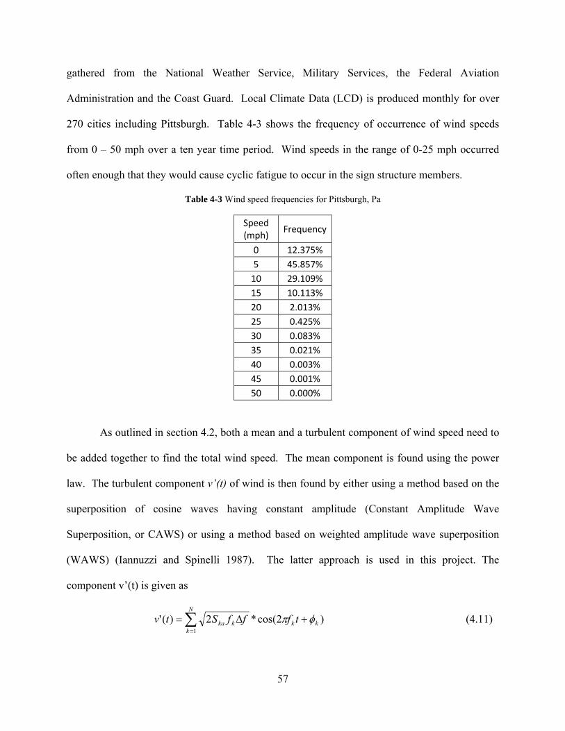
gathered from the National Weather Service, Military Services, the Federal Aviation

Administration and the Coast Guard. Local Climate Data (LCD) is produced monthly for over

270 cities including Pittsburgh. Table 4-3 shows the frequency of occurrence of wind speeds

from 0 – 50 mph over a ten year time period. Wind speeds in the range of 0-25 mph occurred

often enough that they would cause cyclic fatigue to occur in the sign structure members.

Table 4-3 Wind speed frequencies for Pittsburgh, Pa

Speed (mph) 

Frequency

0  12.375% 5  45.857% 10  29.109% 15  10.113% 20  2.013% 25  0.425% 30  0.083% 35  0.021% 40  0.003% 45  0.001% 50  0.000% 

As outlined in section 4.2, both a mean and a turbulent component of wind speed need to

be added together to find the total wind speed. The mean component is found using the power

law. The turbulent component v’(t) of wind is then found by either using a method based on the

superposition of cosine waves having constant amplitude (Constant Amplitude Wave

Superposition, or CAWS) or using a method based on weighted amplitude wave superposition

(WAWS) (Iannuzzi and Spinelli 1987). The latter approach is used in this project. The

component v’(t) is given as

∑=

+Δ=N

kkkkka tfffStv

1)2cos(*2)(' φπ (4.11)

57

where φk is the phase angle randomly distributed between 0 and 2π. After summing the two wind

components, the wind pressure P(t) and the applied force F(t) are given by

2)(21)( tVCtP dρ= (4.12)

(4.13), )()( tAPtF =

where ρ is the air density, V(t) is the combined mean and fluctuating wind velocity, and A is the

gross area over which the pressure is applied.

The above procedure was implemented into a Matlab script wind.m, provided in

Appendix B. Five wind time histories were produced for both the pressure to be applied to the

sign faces and to the truss members. Recall that these have different coefficients of drag which

results in different wind pressures. These pressures are shown in Figure 4-10a and 4-10b. The

process used in the Matlab program is outlined on the next page.

58

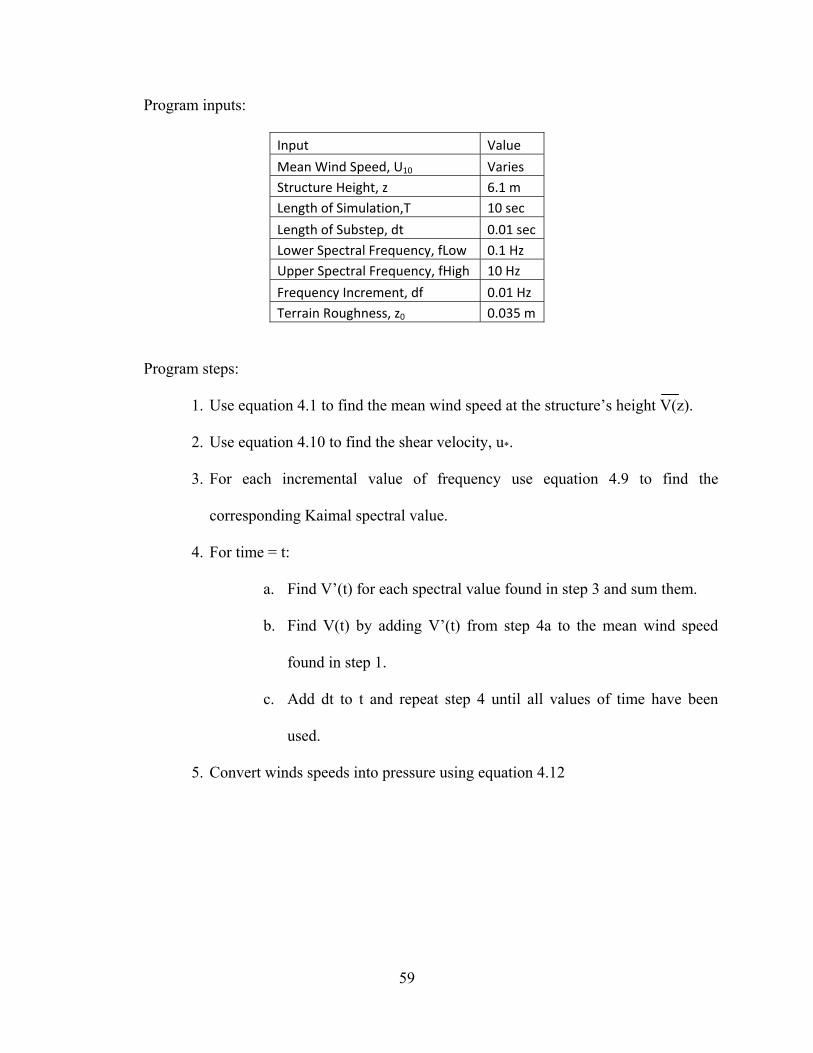
Program inputs:

Input  Value 

Mean Wind Speed, U10  Varies Structure Height, z  6.1 m Length of Simulation,T  10 sec 

Length of Substep, dt  0.01 sec Lower Spectral Frequency, fLow  0.1 Hz Upper Spectral Frequency, fHigh  10 Hz 

Frequency Increment, df  0.01 Hz Terrain Roughness, z0  0.035 m 

Program steps:

1. Use equation 4.1 to find the mean wind speed at the structure’s height V(z).

2. Use equation 4.10 to find the shear velocity, u*.

3. For each incremental value of frequency use equation 4.9 to find the

corresponding Kaimal spectral value.

4. For time = t:

a. Find V’(t) for each spectral value found in step 3 and sum them.

b. Find V(t) by adding V’(t) from step 4a to the mean wind speed

found in step 1.

c. Add dt to t and repeat step 4 until all values of time have been

used.

5. Convert winds speeds into pressure using equation 4.12

59

Figure 4-10a Wind pressures to be applied to signs

Figure 4-11b Wind pressures to be applied to truss elements

60

61

4.5 CONCLUSION

This chapter discussed the ways in which wind could cause vibration and fatigue in highway sign

structures. Past studies proved that galloping and vortex shedding will have little effect on an

overhead structure such as the one in this study. Because this structure supports flat panel signs,

truck induced gusts were also ruled out as having a large affect on fatigue life. This leaves

natural wind as the main cause of fatigue on the structure in this thesis. An algorithm was

produced in order to calculate a 5 second wind pressure time history to be applied to the model,

the results of which are presented in the next chapter.

5.0 FATIGUE LIFE CALCULATION

5.1 INTRODUCTION

This chapter describes the method used to calculate the fatigue life of specific members within

the truss. Figure 5-1 schematically shows how to obtain the fatigue life from a structural model

such as the one described in Chapter 3. Each of the steps shown will be explained in detail in the

next sections. An example fatigue life calculation of a critical member in the structure under

consideration will follow these explanations.

Figure 5-1 Steps in a fatigue life calculation (Ariduru, 2004)

62

AASHTO specifies the use of the stress-life method to calculate fatigue life time. This

method will be explained in the context of an example fatigue life calculation of one of the

critical members in the structure.

5.2 FATIGUE

Fatigue damage occurs when a material or structure is subject to any type of cyclical or repeated

loading. Each cycle inflicts a small amount of damage and as the load repeats the damage begins

to build up. There are two stages of fatigue: initiation and propagation. Damage during the

initiation phase is hard to quantify because it is often caused by microcracks that cannot be easily

detected. On the other hand, damage during the propagation phase is detectable by measuring

the length of the crack (Bannantine 1990). For a fabricated steel structure there are generally

pre-existing cracks or discontinuities, so not much of the fatigue life is attributed to the initiation

phase (Fisher 1998).

Every structure has a fatigue life, or an estimated length of time for which the structure

can stand before failing due to fatigue damage. A structure will fail due to fatigue if a crack is

allowed to grow to the point where it reduces a section’s capacity so much that it cannot carry

the required forces. If fatigue life can be accurately measured, engineers can know when and

where it is important to inspect structures for cracks and these cracks can be mitigated.

63

5.3 THE AASHTO STRESS LIFE METHOD

AASHTO defines fatigue as the damage that may result in fracture after a sufficient number of

stress fluctuations (AASHTO 2004). An infinite life design approach is recommended when

designing for fatigue and the stress-life (S-N) method is suggested for use in quantifying fatigue.

In order to use the S-N method the applied stress must be in the elastic range and the number of

cycles to failure must be high (at least greater than 1000 cycles). As natural wind loading meets

these criteria, the S-N method was used in this study to calculate the fatigue life of the sign

structure.

The basis of this method is the stress-life curves; the curves provided in the AASHTO

bridge manual are shown in Figure 5-2. An S-N curve is a plot of stress range S versus number

of cycles to failure N. The basic equation of each curve is given by:

3i

i SAN = (5.1)

where A is a constant given in the AASHTO 2004 manual that is associated with the member’s

end connection. Si is the stress range acting on the detail at a particular point i and Ni is the

number of cycles of the stress range (Fisher 1998).

According to Figure 5-1, the first step of the fatigue life prediction is modeling the

structure under investigation. This modeling was done using a finite element program and is

detailed in Chapter 3. The second step is the computation of the external force time history

acting on the sign structure. This was described in Chapter 4. Recall that a 10 second wind load

is applied to each sign face and truss and that these wind loads have a base speed of 0-25 mph in

increments of 5 mph. The stress histories for the critical elements are evaluated over a 5 second

period (the final five seconds in the 10 second history) and sampled at 100 Hz. A stress history

64

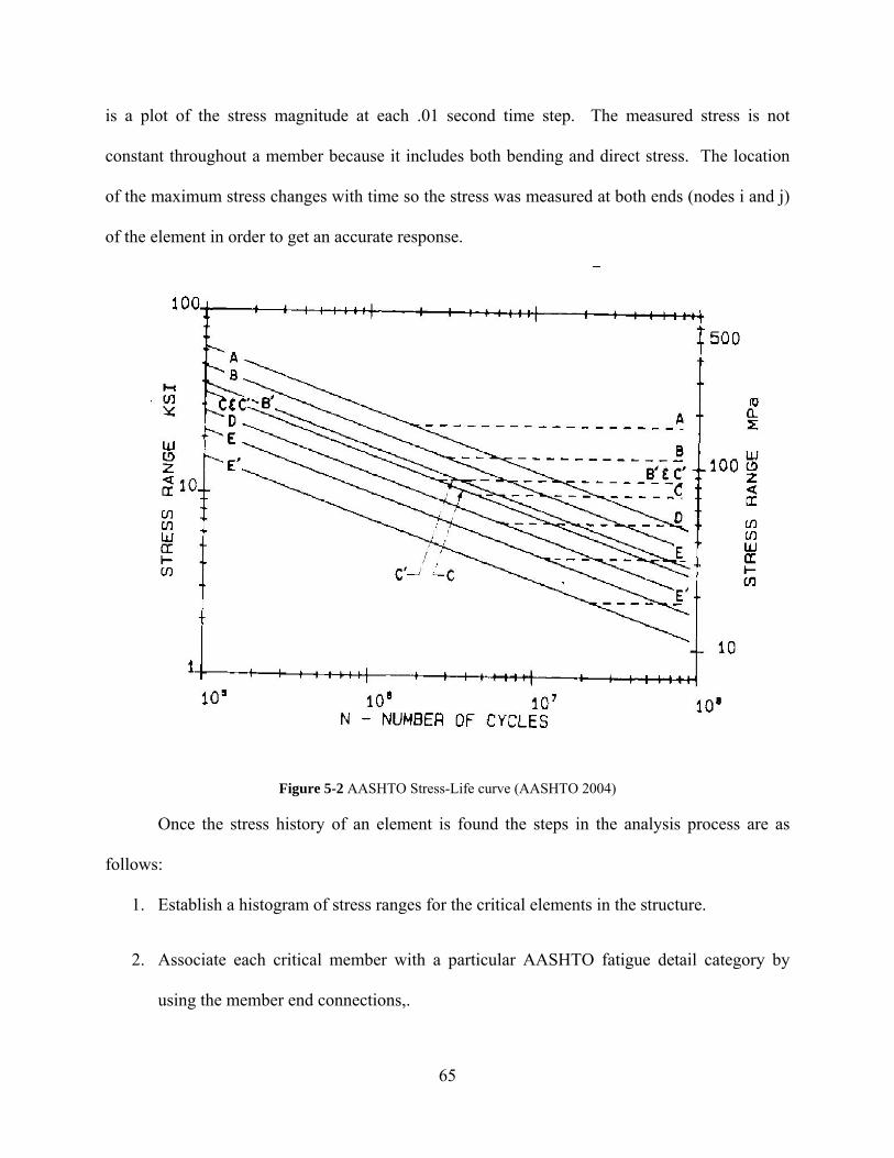
is a plot of the stress magnitude at each .01 second time step. The measured stress is not

constant throughout a member because it includes both bending and direct stress. The location

of the maximum stress changes with time so the stress was measured at both ends (nodes i and j)

of the element in order to get an accurate response.

Figure 5-2 AASHTO Stress-Life curve (AASHTO 2004)

Once the stress history of an element is found the steps in the analysis process are as

follows:

1. Establish a histogram of stress ranges for the critical elements in the structure.

2. Associate each critical member with a particular AASHTO fatigue detail category by

using the member end connections,.

65

3. Use the appropriate S-N diagrams for the AASHTO fatigue detail categories being

considered to calculate fatigue damage of the critical members in the structure.

4. Assess the fatigue life of each critical member. The shortest calculated fatigue life will

be indicative of the structure’s potential service life.

In order to perform step 1 of this process a rainflow counting algorithm is used to

determine the critical stress ranges within each member.

5.3.1 Rainflow Counting Algorithm

Time histories were obtained from the model for five critical elements; the locations of these

elements are shown in Figure 5-3. Critical elements are those elements which would be the first

to fail if fatigue problems exist. These critical elements include three diagonal members on the

front and back face of the truss and two vertical members that connect the top truss chord to the

bottom chord. Diagonal members near the supports in sign structures typically see a lot of load,

so it is important that they are included in the group of critical elements. More discussion of the

critical elements is found in section 5.3.2

Because wind is a non-periodic loading, the structural response has no measureable

constant amplitude or period. In order to measure the damage inflicted upon the structure, the

load’s time history must be reduced into a usable number of constant amplitude cycles. There

are several methods to do this and they all fall under the umbrella term of cycle counting; the

specific method that was employed in this study is called rainflow counting.

66

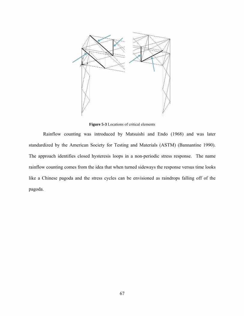
Figure 5-3 Locations of critical elements

Rainflow counting was introduced by Matsuishi and Endo (1968) and was later

standardized by the American Society for Testing and Materials (ASTM) (Bannantine 1990).

The approach identifies closed hysteresis loops in a non-periodic stress response. The name

rainflow counting comes from the idea that when turned sideways the response versus time looks

like a Chinese pagoda and the stress cycles can be envisioned as raindrops falling off of the

pagoda.

67

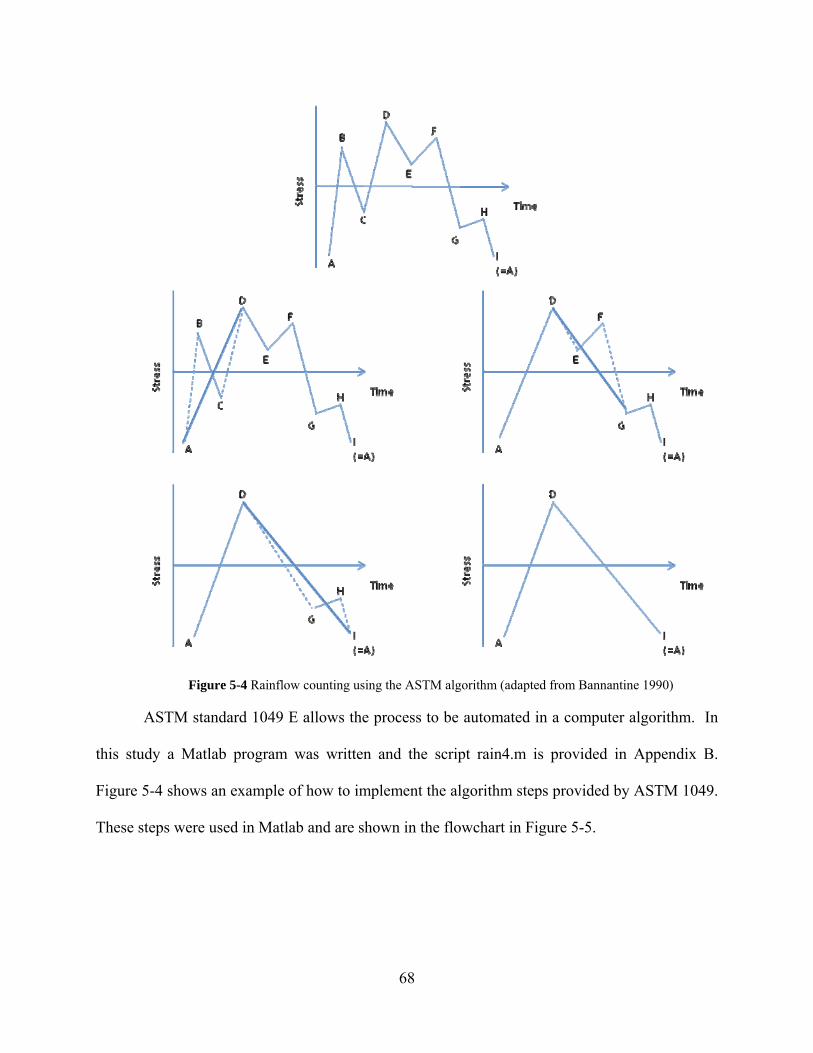
Figure 5-4 Rainflow counting using the ASTM algorithm (adapted from Bannantine 1990)

ASTM standard 1049 E allows the process to be automated in a computer algorithm. In

this study a Matlab program was written and the script rain4.m is provided in Appendix B.

Figure 5-4 shows an example of how to implement the algorithm steps provided by ASTM 1049.

These steps were used in Matlab and are shown in the flowchart in Figure 5-5.

68

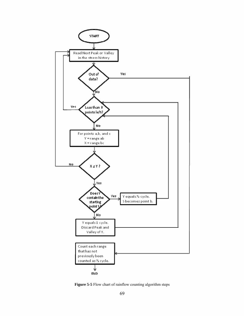
Figure 5-5 Flow chart of rainflow counting algorithm steps

69

5.3.2 Member End Connections

The next step of the analysis procedure uses the AASHTO sign support specifications to

establish the member end connection categories. This subsection describes the process.

Recalling equation 5.1, the value of the constant A is based on the way in which the member

under consideration is connected to the other truss members. The AASHTO sign support

specifications include a table which lists all of the possible fatigue details for support structures

which can be found in Appendix C. This table is broken up into connection type such as

mechanically fastened or fillet-welded. Within the type of connection there are various details

that the particular connection can fall under. Each of these connection details fall into stress

category A, B, B’, C, D, E, E’, ET, or K2. A weaker connection corresponds to a higher letter.

Figure 5-6 shows the location of the various connections in this structure and Table 5-1

shows the connections for the critical members selected in this study. The connection denoted

by a, b, or c in the figure correspond to the detail labeled with a, b, or c in the table.

70

Figure 5-6 Location of connection details within the structure

71

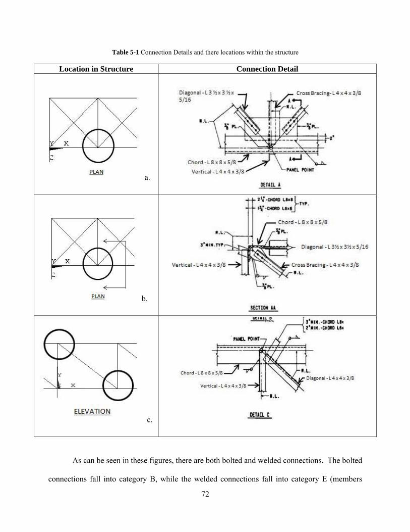
Table 5-1 Connection Details and there locations within the structure

Location in Structure Connection Detail

a.

b.

c.

As can be seen in these figures, there are both bolted and welded connections. The bolted

connections fall into category B, while the welded connections fall into category E (members

72

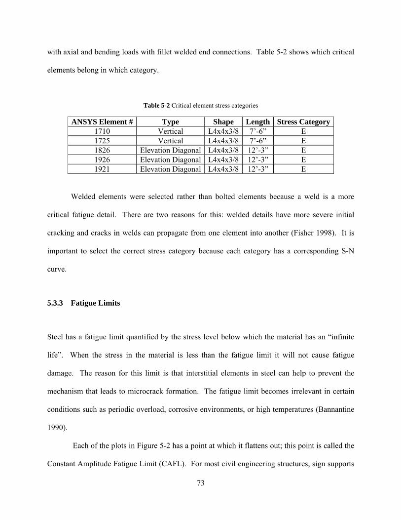
with axial and bending loads with fillet welded end connections. Table 5-2 shows which critical

elements belong in which category.

Table 5-2 Critical element stress categories

ANSYS Element # Type Shape Length Stress Category1710 Vertical L4x4x3/8 7’-6” E 1725 Vertical L4x4x3/8 7’-6” E 1826 Elevation Diagonal L4x4x3/8 12’-3” E 1926 Elevation Diagonal L4x4x3/8 12’-3” E 1921 Elevation Diagonal L4x4x3/8 12’-3” E

Welded elements were selected rather than bolted elements because a weld is a more

critical fatigue detail. There are two reasons for this: welded details have more severe initial

cracking and cracks in welds can propagate from one element into another (Fisher 1998). It is

important to select the correct stress category because each category has a corresponding S-N

curve.

5.3.3 Fatigue Limits

Steel has a fatigue limit quantified by the stress level below which the material has an “infinite

life”. When the stress in the material is less than the fatigue limit it will not cause fatigue

damage. The reason for this limit is that interstitial elements in steel can help to prevent the

mechanism that leads to microcrack formation. The fatigue limit becomes irrelevant in certain

conditions such as periodic overload, corrosive environments, or high temperatures (Bannantine

1990).

Each of the plots in Figure 5-2 has a point at which it flattens out; this point is called the

Constant Amplitude Fatigue Limit (CAFL). For most civil engineering structures, sign supports

73

included, there can be stress ranges both above and below the CAFL and there are two ways to

handle this situation. First, it can be assumed that all of the stress ranges will cause crack

propagation. This is a very conservative assumption because laboratory tests have proven that

this is not the case. The other option is to assume that not all ranges will cause immediate crack

propagation. The AASHTO bridge design specification states that when the design stress range

is less than one-half of the CAFL, the detail will theoretically provide infinite life. This is the

way in which the situation of having stress ranges both above and below the CAFL will be

handled in this project. Table 5-3 shows the CAFL values for each detail category as specified

by AASHTO.

74

Table 5-3 Constant amplitude fatigue limits (AASHTO, 2001)

Detail Category CAFL (ksi)A 24B 16B’ 12C 10D 7E 4.5E’ 2.6

ET 1.2K 1

The bolted connections (category B) and the welded connections (category E) in the

structure currently under analysis have very different CAFLs. It will take a much higher stress to

cause fatigue in the bolted connections than in the welded connections. For this reason it is

likely that the vertical and elevation diagonal members will control the fatigue life of the sign

support structure.

5.3.4 The Palmgren-Miner Rule of Linear Damage Accumulation

Step 3 of the analysis procedure involves calculating the fatigue damage in the critical members.

Because there are many varying stress ranges, a damage summing method is used. Commonly

known as Miner’s rule (or the Palmgren-Miner rule), the linear damage summing method used in

this project was first proposed by Palmgren in 1924 and further developed by Miner in 1945

(Bannantine 1990). This method assumes that the fraction of damage Di that results from a

specific stress range Si, is a linear function of the number of cycles that take place at that stress

range ni. The relationship between these values is given as:

i

ii N

nD = (5.2)

75

∑= iDD (5.3)

where Ni is the number of cycles it would take to cause failure (the fatigue life) at stress range i

The value of Ni can be found using equation (5.1).

If there is only one cycle of a particular stress range, D is given by 1/N. Once the

damage for each individual stress range is found, the total damage D can be found by summing

these individual damages as shown in equation 5.3. According to the Palmgren-Miner Rule,

failure occurs when the damage D is equal to 1.

Tests have been undertaken in order to verify the Palmgren-Miner rule (Bannantine

1990). In these tests an initial stress, S1, is applied for a certain number of cycles, and this is

followed by the application of a second stress level, S2, until failure. For S1 >S2, the test is

known as high-low and for S1<S2 it is a low-high test. When Miner originally performed this

test he found that failure occurred when D was between 0.61 and 1.45, within which his

proscribed value of 1 falls. The majority of most other tests have found values ranging from 0.5

to 2.0, with an average value close to 1. Though these types of two step tests do not well mimic

the randomly varying loads seen in the field, tests using several random stress histories have also

been shown to correlate with the stated failure value of 1 (Bannantine 1990).

The Palmgren-Miner approach has disadvantages. The most often cited limitation is that

it is a linear method; it assumes that all cycles of a given stress range cause the same amount of

damage regardless of when they occur in a structure’s lifetime. Also, the method assumes that

the presence of one stress range does not affect the damage caused by a different stress range.

Despite these limitations, AASHTO specifies the use of the Palmgren-Miner rule to account for

cumulative damage.

76

5.4 FATIGUE LIFE ANALYSIS

This section will provide the fatigue life of all of the critical members in the structure.

5.4.1 Wind Probability

As described in the previous chapter, base wind speeds of 0-25 mph were used to

simulate the action of wind load on the structure. Weather data from the NCDC were used to

measure the probability of each of these speeds occurring. The Pittsburgh LCD is collected at

the Pittsburgh International Airport and provides an hourly measurement of wind speed and

direction. The wind speed is measured over a 1-minute averaging period; the speed is not a

maximum value during the hour, but rather the speed measured at the chosen time.

In the study data collected between January 1999 and December 2008 was used. Once all

of the wind speeds were collected, they were placed into 5 mph bins with the center point of each

bin being a value from 0-25 mph spaced at increments of 5. For example, the bin containing the

value of 10 mph includes all wind speeds between 7.5 and 12.5 mph. The only exception to this

rule is the bin ranging from >0 – 7.5 mph. Likewise, the directions were also broken up into bins

containing the 4 cardinal directions and the 4 primary inter-cardinal directions. Figures 5-7 and

5-8 show the resulting histograms. The wind speed histogram shows a positively skewed

distribution with the maximum number of speeds occurring in the 5 mph bin. The directional

frequency shows that the prevailing wind flows along west direction.

77

Figure 5-7 Frequency of wind speeds in Pittsburgh, Pa

Figure 5-8 Frequency of wind direction in Pittsburgh, Pa

After compiling all of the wind data, a basic statistical analysis was performed in order to

determine the probability of occurrence of a particular speed or direction. Since there are two

variables that must occur, speed and direction, their probability can either be analyzed as a joint

probability or an independent probability. A joint probability is the probability that both events

A and B will occur, while an independent probability is the probability that event A will occur.

The joint probability is based on conditional probability, which is the probability that A occurs

78

given that B has taken place (or will take place). Both of these cases were analyzed, however

only the joint probability is used so that is what is presented here. It was decided that the

direction of the wind flow is dependent on the wind speed (or vice versa) because they are given

as one entity by the NCDC data. The equation used to find the joint probability is given by:

)|(*)()|(*)()( ABPAPBAPBPBAP ==∩ (5.5)

where, P(A∩B) is the joint probability, P(A) is the independent probability of A, and a

conditional probability is written as P(A|B) and read “probability of A given B.”

This formula can be interpreted by understanding that the probability that both A and B

take place requires two things to happen: first event A takes place, and then event B takes place

on the condition that A has already occurred.

In order to find the joint probability of the wind speed and direction from the NCDC data

equation 5.5 is used. Wind speed is event A and wind direction is event B. The individual P(A)

and P(B) are known from the histograms shown in Figures 5-7 and 5-8. In order to find the

conditional probabilities, the partnered daily speed and direction were sorted into bins falling

into the 5 mph increments discussed earlier. The results of this procedure are presented in the

histograms in Figure 5-9. The data shown in these histograms is P(B|A) and after it is found

equation 5.5 can be used to produce the joint probability. This process was also done using the

wind speed as event B and the wind direction as event A. P(A∩B) = P(B∩A), so the same

results should be found regardless of which variable is called event A or B. Table 5-4 and Table

5-5 present the conditional and joint probabilities respectively for the case where event A is wind

speed. Likewise, Table 5-6 and Table 5-7 present the conditional and joint probabilities

respectively where event A is wind direction.

79

Figure 5-9 Directional Probabilities given that a certain wind speed has occurred

80

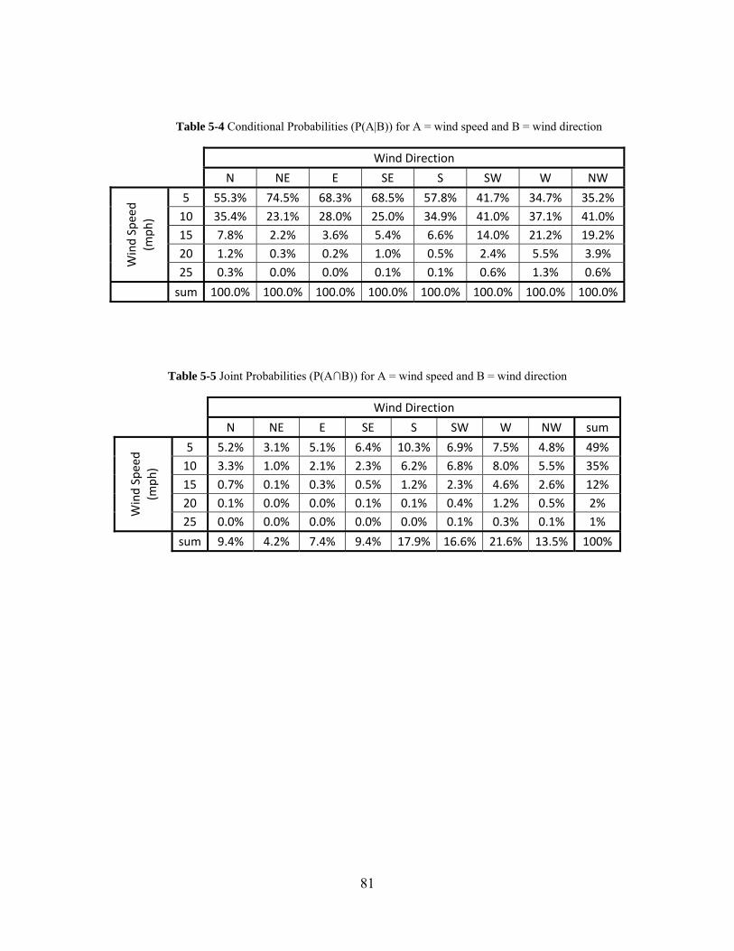
81

Table 5-4 Conditional Probabilities (P(A|B)) for A = wind speed and B = wind direction

 Wind Direction 

N  NE  E  SE  S  SW  W  NW 

Wind Speed 

(mph

) 

5  55.3%  74.5%  68.3%  68.5%  57.8%  41.7%  34.7%  35.2% 10  35.4%  23.1%  28.0%  25.0%  34.9%  41.0%  37.1%  41.0% 15  7.8%  2.2%  3.6%  5.4%  6.6%  14.0%  21.2%  19.2% 20  1.2%  0.3%  0.2%  1.0%  0.5%  2.4%  5.5%  3.9% 25  0.3%  0.0%  0.0%  0.1%  0.1%  0.6%  1.3%  0.6% 

sum  100.0%  100.0% 100.0% 100.0% 100.0% 100.0% 100.0%  100.0%

Table 5-5 Joint Probabilities (P(A∩B)) for A = wind speed and B = wind direction

 Wind Direction 

N  NE  E  SE  S  SW  W  NW  sum 

Wind Speed 

(mph

) 

5  5.2%  3.1%  5.1%  6.4%  10.3% 6.9%  7.5%  4.8%  49% 10  3.3%  1.0%  2.1%  2.3%  6.2%  6.8%  8.0%  5.5%  35% 15  0.7%  0.1%  0.3%  0.5%  1.2%  2.3%  4.6%  2.6%  12% 20  0.1%  0.0%  0.0%  0.1%  0.1%  0.4%  1.2%  0.5%  2% 25  0.0%  0.0%  0.0%  0.0%  0.0%  0.1%  0.3%  0.1%  1% 

sum  9.4%  4.2%  7.4%  9.4%  17.9% 16.6% 21.6%  13.5%  100% 

Table 5-6 Conditional Probabilities (P(A|B)) for A = wind direction and B = wind speed

 Wind Direction 

N  NE  E  SE  S  SW  W  NW  sum 

Wind Speed 

(mph

) 

5  10.6%  6.3%  10.3% 13.0% 21.0% 14.1% 15.2%  9.6%  100% 10  9.4%  2.7%  5.9%  6.6%  17.7% 19.3% 22.7%  15.7%  100% 15  6.0%  0.7%  2.2%  4.1%  9.5%  19.0% 37.3%  21.1%  100% 20  4.6%  0.4%  0.6%  4.0%  3.8%  16.1% 48.7%  21.6%  100% 25  4.8%  0.0%  0.2%  1.0%  2.5%  20.7% 54.7%  16.1%  100% 

Table 5-7 Joint Probabilities (P(A∩B)) for A = wind direction and B = wind speed

 Wind Direction 

N  NE  E  SE  S  SW  W  NW  sum 

Wind Speed 

(mph

) 

5  5.2%  3.1%  5.1%  6.4%  10.4% 7.0%  7.5%  4.8%  49% 10  3.3%  1.0%  2.1%  2.3%  6.2%  6.8%  8.0%  5.5%  35% 15  0.7%  0.1%  0.3%  0.5%  1.2%  2.3%  4.6%  2.6%  12% 20  0.1%  0.0%  0.0%  0.1%  0.1%  0.4%  1.2%  0.5%  2% 25  0.0%  0.0%  0.0%  0.0%  0.0%  0.1%  0.3%  0.1%  1% 

sum  9.4%  4.2%  7.4%  9.4%  17.9% 16.6% 21.6%  13.5%  100.0%

82

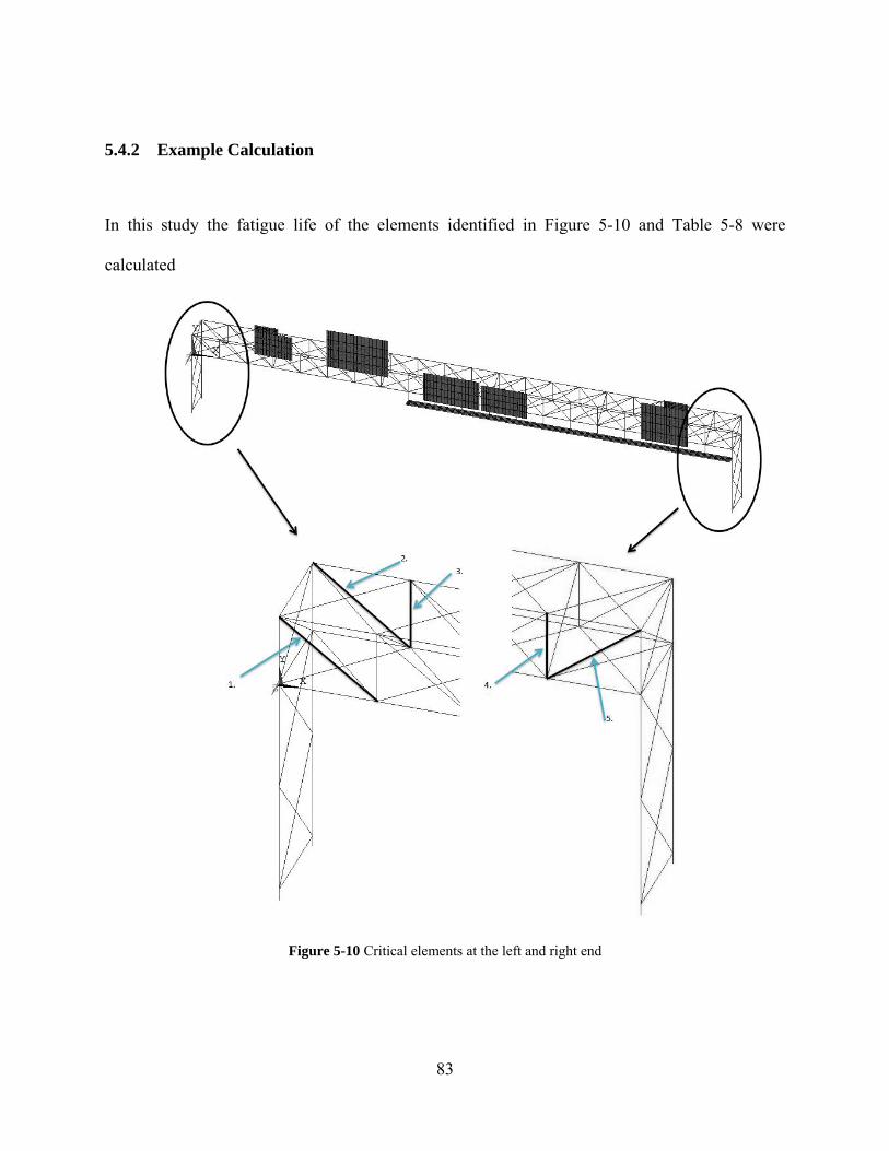
5.4.2 Example Calculation

In this study the fatigue life of the elements identified in Figure 5-10 and Table 5-8 were

calculated

Figure 5-10 Critical elements at the left and right end

83

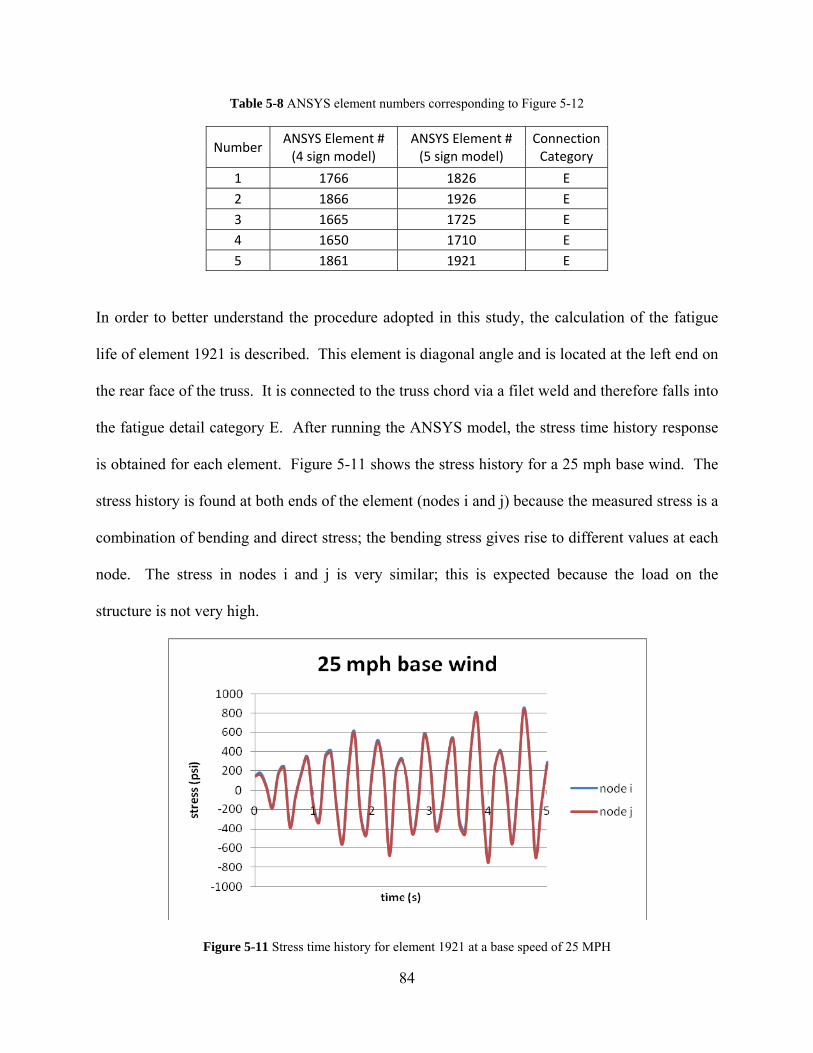
Table 5-8 ANSYS element numbers corresponding to Figure 5-12

Number ANSYS Element #    (4 sign model) 

ANSYS Element #    (5 sign model) 

Connection Category 

1  1766  1826  E 2  1866  1926  E 3  1665  1725  E 4  1650  1710  E 5  1861  1921  E 

In order to better understand the procedure adopted in this study, the calculation of the fatigue

life of element 1921 is described. This element is diagonal angle and is located at the left end on

the rear face of the truss. It is connected to the truss chord via a filet weld and therefore falls into

the fatigue detail category E. After running the ANSYS model, the stress time history response

is obtained for each element. Figure 5-11 shows the stress history for a 25 mph base wind. The

stress history is found at both ends of the element (nodes i and j) because the measured stress is a

combination of bending and direct stress; the bending stress gives rise to different values at each

node. The stress in nodes i and j is very similar; this is expected because the load on the

structure is not very high.

Figure 5-11 Stress time history for element 1921 at a base speed of 25 MPH

84

Time histories were found for all of the base wind speeds from 5 to 25 mph. The next

step was to use the matlab file rain4.m to find the complete stress cycles in this time history.

Table 5-9 lists the stress values calculated at the completion of each cycle. Recall that if a stress

range contains the starting point s of the distribution when using the rainflow method, that stress

range only counts as a half a cycle rather than a full cycle. Those ranges for which this is the

case are highlighted in Table 5-9. The complete calculation of these stress ranges is shown in

Appendix B.

Table 5-9 Stress ranges in psi in element 1921 at 25 mph

Stress at i  Stress at j 

349.78 345.09414.83 410.68608.54 605.85649.56 657.64775.23 766.49777.04 779.58905.54 927.54945.49 936.50946.48 967.84966.74 973.28995.23 1022.57

1462.67 1466.41

For fatigue detail E the CAFL fatigue threshold set by AASHTO is 4500 psi (AASHTO

2001). According to the stress life method, only those stress ranges with a value greater than

half of this threshold will cause fatigue damage. In the case of an E detail, only values above

2250 psi will be considered. None of the stress ranges in Table 5-9 are above this CAFL, but for

the sake of this example they will all be used to show how damage is calculated.

Next, the number of cycles (N) required to induce damage was calculated by using the S-

N curves shown in Figure 5-2. Equation 5.1 gave the equation of the curve:

85

3i

i SAN = (5.1)

For fatigue category E the constant A is equal to 11 x 108 ksi3 and the damage (D) caused by one

cycle can then be found by dividing 1 by N:

Table 5-10 The damage at node i and j of element 1921 caused by a 25 mph wind

node i  node j 

Si (psi) ni 

(cycles) Ni 

(cycles) Di 

 Si (psi) 

ni (cycles) 

Ni (cycles) 

Di 

349.78  0.5  2.57E+10  1.95E‐11 345.09  0.5  2.68E+10  1.87E‐11414.83  0.5  1.54E+10  3.24E‐11 410.68  0.5  1.59E+10  3.15E‐11608.54  0.5  4.88E+09  1.02E‐10 605.85  0.5  4.95E+09  1.01E‐10649.56  1  4.01E+09  2.49E‐10 657.64  1  3.87E+09  2.59E‐10775.23  0.5  2.36E+09  2.12E‐10 766.49  0.5  2.44E+09  2.05E‐10777.04  1  2.34E+09  4.27E‐10 779.58  1  2.32E+09  4.31E‐10905.54  1  1.48E+09  6.75E‐10 927.54  1  1.38E+09  7.25E‐10945.49  1  1.30E+09  7.68E‐10 936.50  0.5  1.34E+09  3.73E‐10946.48  0.5  1.30E+09  3.85E‐10 967.84  1  1.21E+09  8.24E‐10966.74  1  1.22E+09  8.21E‐10 973.28  1  1.19E+09  8.38E‐10995.23  1  1.12E+09  8.96E‐10 1022.57 1  1.03E+09  9.72E‐101462.67  1  3.52E+08  2.84E‐09 1466.41 1  3.49E+08  2.87E‐09

ΣD  7.43E‐09 ΣD  7.65E‐09

The Palmgren-Miner rule states that the total damage can be found by summing all of the

individual damages. In the case of node i the total damage is 7.43 x 10-9 and is 7.65 x 10-9 for

node j. These values are unitless.

In order to turn these damages into fatigue lives the wind probability data given in section

5.4.1 is needed. Because the sign is oriented such that wind flowing in the north and south

direction hits it, only those probabilities are needed. Table 5-11, which presents these

probabilities, was extracted from Table 5-7.

86

Table 5-11 Probability of wind blowing in a certain direction for a certain speed

Probability of northern wind

Probability of southern wind

win

d sp

eed

(mph

)

5 5.210%  10.353% 

10 3.338%  6.245% 

15 0.738%  1.173% 

20 0.112%  0.094% 

25 0.025%  0.013% 

Because the load was applied to the model for a 5 second time period, the number of 5

second cycles in one year must be found:

200,307,6sec5/sec86400*365 =⎟⎟⎠

⎞⎜⎜⎝

⎛dayyear

days

The number of 5 second cycles/year of each wind speed in both the north and south direction can

be found by multiplying the directional probability by 6,307,200 cycles/year. These values are

given in Table 5-12.

Table 5-12 Number of 5 second cycles per year for given direction and speed

  5 second 

cycles/year (N) 5 second 

cycles/year (S) 

wind speed 

(mph

) 

5  328,577  653,000 10  210,537  393,898 15  46,521  73,971 20  7,084  5,926 25  1,567  817 

The damage caused in one year is then found by multiplying the summed damage at a particular

wind speed by the number of 5 second cycles/year of the corresponding wind speed and

direction. For example, the damage caused by a 25 mph wind in the northern direction at node i

of element 1921 is given by:

87

⎟⎟⎠

⎞⎜⎜⎝

⎛⋅=⎟⎟

⎠

⎞⎜⎜⎝

⎛⎟⎟⎠

⎞⎜⎜⎝

⎛⋅ −−

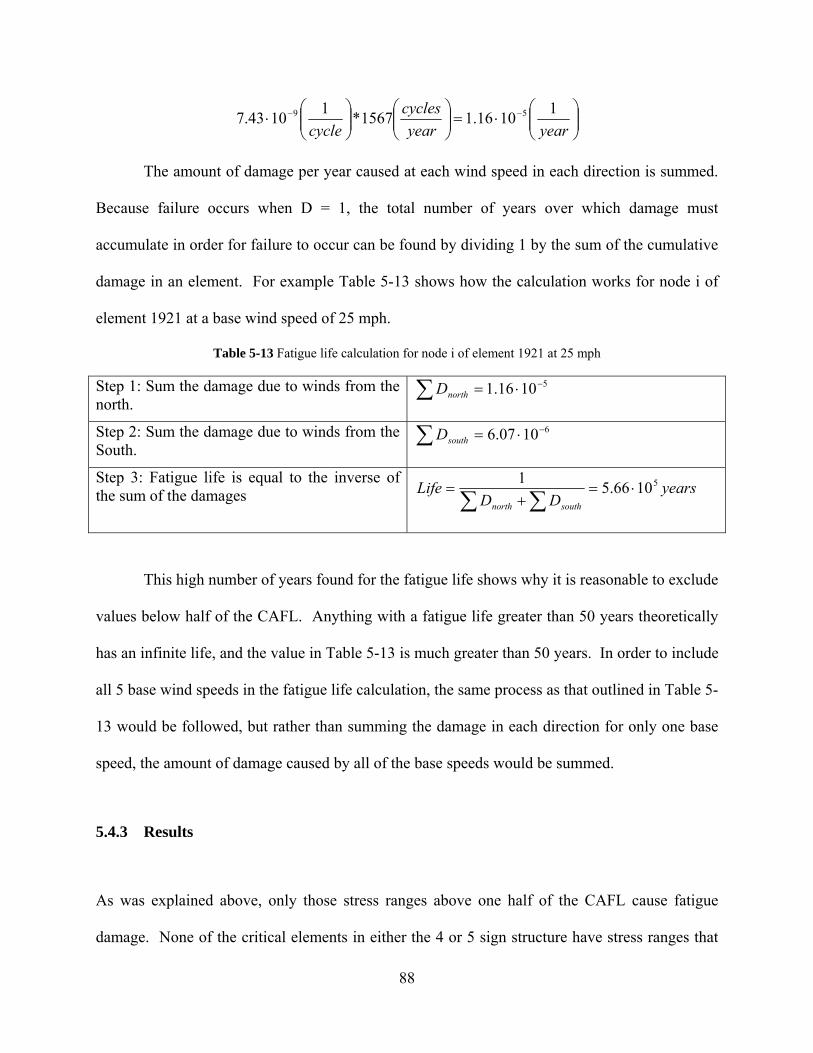
yearyearcycles

cycle11016.11567*11043.7 59

The amount of damage per year caused at each wind speed in each direction is summed.

Because failure occurs when D = 1, the total number of years over which damage must

accumulate in order for failure to occur can be found by dividing 1 by the sum of the cumulative

damage in an element. For example Table 5-13 shows how the calculation works for node i of

element 1921 at a base wind speed of 25 mph.

Table 5-13 Fatigue life calculation for node i of element 1921 at 25 mph

Step 1: Sum the damage due to winds from the north.

∑ −⋅= 51016.1northD

Step 2: Sum the damage due to winds from the South.

∑ −⋅= 61007.6southD

Step 3: Fatigue life is equal to the inverse of the sum of the damages years

DDLife

southnorth

51066.51⋅=

+=∑ ∑

This high number of years found for the fatigue life shows why it is reasonable to exclude

values below half of the CAFL. Anything with a fatigue life greater than 50 years theoretically

has an infinite life, and the value in Table 5-13 is much greater than 50 years. In order to include

all 5 base wind speeds in the fatigue life calculation, the same process as that outlined in Table 5-

13 would be followed, but rather than summing the damage in each direction for only one base

speed, the amount of damage caused by all of the base speeds would be summed.

5.4.3 Results

As was explained above, only those stress ranges above one half of the CAFL cause fatigue

damage. None of the critical elements in either the 4 or 5 sign structure have stress ranges that

88

meet this criterion so each element can be said to have an infinite life. This makes sense because

these structures are designed to withstand dynamic fatigue inducing forces, so unless they are

incorrectly designed we should expect them to have an infinite life.

In order to make a comparison between the 4 and 5 sign model, the complete fatigue life

calculations shown in the example calculation of section 5.4.2 were carried out for all base wind

speeds. Even though all of the stress ranges were below the CAFL, they were all used to find the

fatigue lives shown in Tables 5-14 and 5-15, which show the life results for the 4 and 5 sign

model respectively. The tables only include the diagonal critical members, though the vertical

members would follow the same trend. The fatigue life is longer for all of the members in the

four sign model. This makes sense because there is less loading applied to the truss. The stress

ranges in the members in the four sign model were much lower than those in the five sign model,

thus leading to a longer lifetime.

Table 5-14 Fatigue life for the four sign model

Total Damage          5 mph  10 mph  15 mph  20 mph  25 mph  sum  Life (years)

1826 i 

north  4.15E‐10 9.17E‐09 2.84E‐08 1.61E‐07 5.39E‐08 4.78E‐07  2,092,343 

south  8.25E‐10 1.72E‐08 4.51E‐08 1.34E‐07 2.81E‐08 

j north  3.88E‐10 7.57E‐09 3.22E‐08 4.24E‐08 5.31E‐08 

2.65E‐07  3,775,050 south  7.72E‐10 1.42E‐08 5.11E‐08 3.55E‐08 2.77E‐08 

1921 i 

north  1.93E‐10 3.30E‐08 9.72E‐08 2.24E‐07 1.09E‐07 9.25E‐07  1,081,096 

south  3.83E‐10 6.18E‐08 1.55E‐07 1.88E‐07 5.68E‐08 

j north  3.05E‐10 3.40E‐08 8.13E‐08 2.63E‐07 1.11E‐07 

9.61E‐07  1,041,087 south  3.66E‐10 6.36E‐08 1.29E‐07 2.20E‐07 5.81E‐08 

1926 i 

north  3.52E‐10 5.51E‐08 7.53E‐08 4.72E‐08 3.51E‐07 9.74E‐07  1,026,406 

south  6.99E‐10 1.03E‐07 1.20E‐07 3.95E‐08 1.83E‐07 

j north  2.44E‐10 6.53E‐08 2.48E‐08 3.96E‐07 4.18E‐07 

1.62E‐06  618,741 south  4.85E‐10 1.22E‐07 3.95E‐08 3.32E‐07 2.18E‐07 

89

Table 5-15 Fatigue life for the five sign model

Total Damage          5 mph  10 mph  15 mph  20 mph  25 mph  sum  Life (years) 

1826 i 

north  1.29E‐09 5.56E‐08 1.76E‐07 2.53E‐07 1.20E‐07 1.27E‐06 789,506 

south  2.57E‐09 1.04E‐07 2.80E‐07 2.12E‐07 6.25E‐08 

j north  1.33E‐09 2.15E‐08 1.60E‐07 2.14E‐07 1.23E‐07 

1.12E‐06 892,939 south  2.65E‐09 9.99E‐08 2.55E‐07 1.79E‐07 6.41E‐08 

1921 i 

north  1.61E‐08 2.82E‐06 4.55E‐07 2.20E‐06 1.16E‐05 2.68E‐05 37,322 

south  3.20E‐08 9.92E‐07 7.23E‐07 1.84E‐06 6.07E‐06 

j north  1.64E‐08 2.95E‐06 4.56E‐07 2.61E‐06 1.20E‐05 

3.27E‐05 30,558 south  3.25E‐08 5.52E‐06 7.25E‐07 2.19E‐06 6.25E‐06 

1926 i 

north  2.56E‐09 2.81E‐07 4.58E‐07 1.79E‐06 3.21E‐07 5.77E‐06 173,240 

south  5.08E‐09 5.26E‐07 7.29E‐07 1.50E‐06 1.67E‐07 

j north  2.44E‐09 2.65E‐07 5.21E‐07 2.14E‐06 2.77E‐07 

6.47E‐06 154,486 south  4.86E‐09 4.95E‐07 8.28E‐07 1.79E‐06 1.44E‐07 

Though the results show that the structure will have an infinite life, it cannot be 100%

concluded that the structure will never sustain any fatigue damage. This analysis method

assumes that the connections between members are made to code, which may not be the case. A

survey sent to all of the 50 state’s and Canadian province’s departments of transportation in 2008

(Rizzo et al. 2008) asked the respondents to identify common problems that have occurred in

sign structures within their jurisdiction. Some of these problems include cracks in welds and

loose or missing bolts. A weakened connection like this could result in the occurrence of fatigue

damage. Members with welded connections are still the most critical elements due to their lower

CAFL and should be closely checked for fatigue cracks when inspections are performed.

Specifically, the members closest to the truss ends should be directly monitored.

It should be pointed out that the fatigue life predictions estimated by Ginal (2003) and Li

(2005) were very different from one another. The truss with a flat panel sign in Ginal was a

trichord overhead structure and Li performed an analysis on a box chord truss. Unlike this

90

current project and Li’s project, Ginal included truck induced wind gusts and the structure’s self

weight in his investigation. In the case of Ginal the lowest fatigue life in a diagonal member was

4 years whereas Li found that the connection between a diagonal and truss chord had an infinite

life. The method of using wind probabilities in the present study to find fatigue lives was based

on the method used by Ginal, though the results found here are more consistent with those

presented by Li. Despite this, it is difficult to compare the three studies because the trusses in

each were of varying lengths and had different sign attachments. Additionally, the truss

members in the current study were angles whereas those in both previous studies were tubular

members. Tubular members have a different fatigue detail category with a lower CAFL

(category ET) and therefore smaller stress values can cause damage.

5.5 CONCLUSION

This chapter presented the method for determining the fatigue life of members within the model.

This method has been used by past researchers doing similar projects. By building a finite

element model, finding the stress time history and using a cycle counting method to determine

complete stress cycles, and then using the Palmgren Miner rule of linear damage accumulation

the fatigue life can be found. The results found in this chapter are for an undamaged structure;

the next chapter will discuss what happens when a structure in the field is damaged.

91

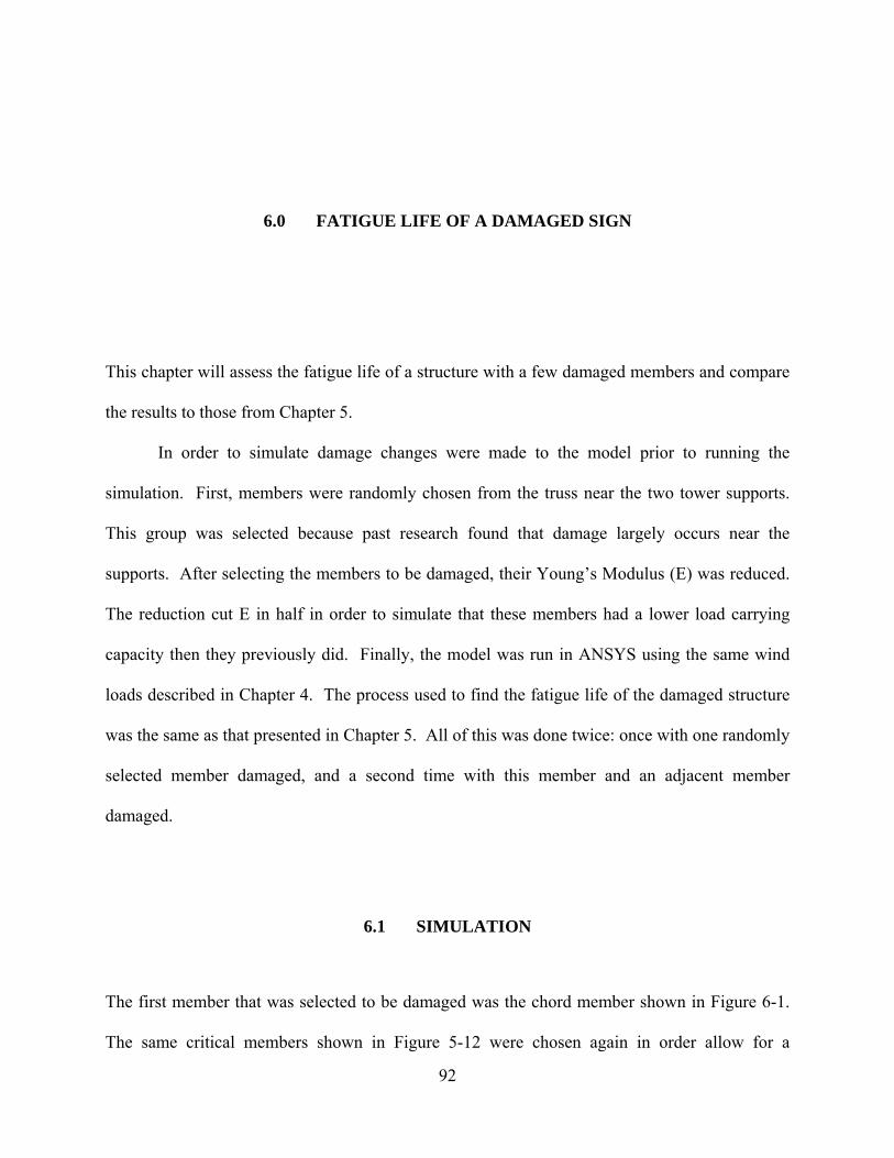
6.0 FATIGUE LIFE OF A DAMAGED SIGN

This chapter will assess the fatigue life of a structure with a few damaged members and compare

the results to those from Chapter 5.

In order to simulate damage changes were made to the model prior to running the

simulation. First, members were randomly chosen from the truss near the two tower supports.

This group was selected because past research found that damage largely occurs near the

supports. After selecting the members to be damaged, their Young’s Modulus (E) was reduced.

The reduction cut E in half in order to simulate that these members had a lower load carrying

capacity then they previously did. Finally, the model was run in ANSYS using the same wind

loads described in Chapter 4. The process used to find the fatigue life of the damaged structure

was the same as that presented in Chapter 5. All of this was done twice: once with one randomly

selected member damaged, and a second time with this member and an adjacent member

damaged.

6.1 SIMULATION

The first member that was selected to be damaged was the chord member shown in Figure 6-1.

The same critical members shown in Figure 5-12 were chosen again in order allow for a

92

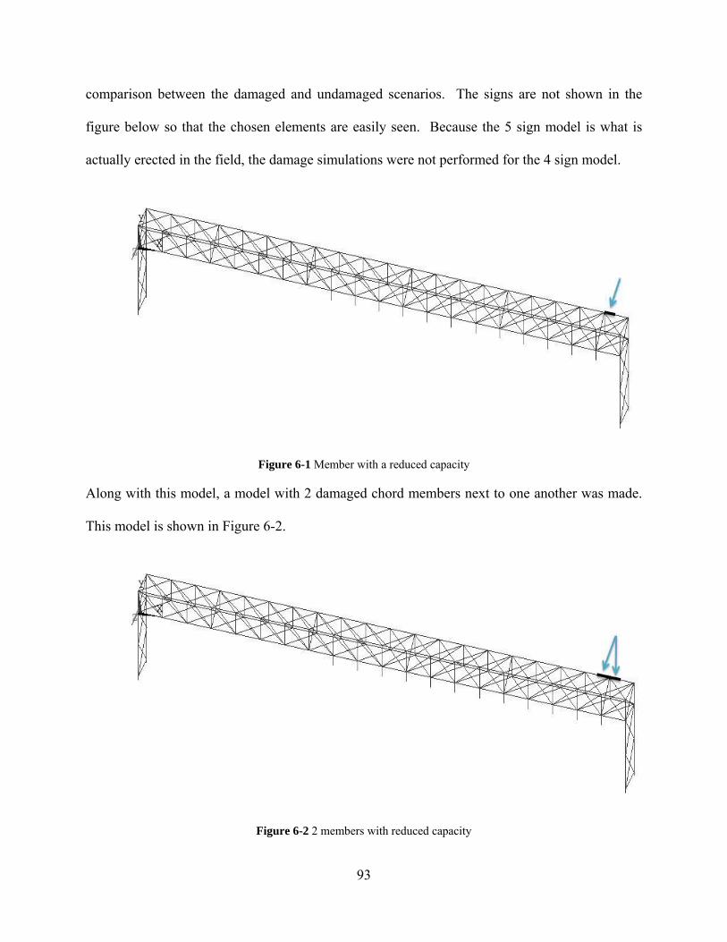
comparison between the damaged and undamaged scenarios. The signs are not shown in the

figure below so that the chosen elements are easily seen. Because the 5 sign model is what is

actually erected in the field, the damage simulations were not performed for the 4 sign model.

Figure 6-1 Member with a reduced capacity

Along with this model, a model with 2 damaged chord members next to one another was made.

This model is shown in Figure 6-2.

Figure 6-2 2 members with reduced capacity

93

6.1.1 Results

The fatigue lives of critical members in these two models were found. Like the pristine model,

the fatigue lives are once again infinite. This shows that the structure is redundant enough to

withstand some minor damage without it impacting the overall fatigue life of the structure. As

was done in Chapter 5, fatigue lives of critical elements were found even though all of the stress

ranges were below the CAFL in order to compare the results. Table 6-1 shows the results of the

model with 1 element damaged, and Table 6-2 shows the results with 2 elements damaged.

Comparing the two tables shows that a slight reduction in lifetime occurs when a second element

is damaged. Additionally, the shortest fatigue life in element 1921 in the pristine case presented

in chapter 5 was 30,558 years, while it is 18,673 years and 18,666 years in the case when 1 or 2

elements are damaged. Thus, damage in the chord members will impact fatigue life in critical

members, but not enough to result in their failure.

94

Table 6-1 Fatigue life with 1 element damaged

Total Damage          5 mph  10 mph  15 mph  20 mph  25 mph  sum  Life (years) 

1826 i 

north  8.38E‐10 6.60E‐08 9.48E‐08 4.48E‐07 2.91E‐07 1.70E‐06  587,021 

south  1.67E‐09 1.24E‐07 1.51E‐07 3.75E‐07 1.52E‐07 

j north  8.49E‐10 7.02E‐08 9.08E‐08 4.32E‐07 3.53E‐07 

1.77E‐06  565,003 south  1.02E‐09 1.31E‐07 1.44E‐07 3.62E‐07 1.84E‐07 

1921 i 

north  9.15E‐09 2.89E‐06 5.08E‐07 2.35E‐06 1.64E‐05 3.89E‐05  25,692 

south  1.82E‐08 5.41E‐06 8.08E‐07 1.96E‐06 8.56E‐06 

j north  1.78E‐08 3.88E‐06 5.02E‐07 1.79E‐06 2.48E‐05 

5.36E‐05  18,673 south  3.53E‐08 7.26E‐06 7.98E‐07 1.50E‐06 1.29E‐05 

1926 i 

north  7.44E‐10 2.70E‐07 5.17E‐07 2.59E‐06 3.92E‐07 7.46E‐06  133,990 

south  1.48E‐09 5.05E‐07 8.22E‐07 2.16E‐06 2.04E‐07 

j north  7.58E‐10 2.57E‐07 5.15E‐07 2.54E‐06 3.81E‐07 

7.31E‐06  136,742 south  1.51E‐09 4.81E‐07 8.19E‐07 2.12E‐06 1.99E‐07 

Table 6-2 Fatigue life with 2 elements damaged

Total Damage          5 mph  10 mph  15 mph  20 mph  25 mph  sum  Life (years) 

1826 i 

north  8.42E‐10 6.62E‐08 9.60E‐08 4.53E‐07 2.86E‐07 1.71E‐06  585,374 

south  1.67E‐09 1.24E‐07 1.53E‐07 3.79E‐07 1.49E‐07 

j north  8.52E‐10 6.91E‐08 1.59E‐07 4.35E‐07 4.25E‐07 

2.06E‐06  485,971 south  1.69E‐09 1.29E‐07 2.52E‐07 3.64E‐07 2.22E‐07 

1921 i 

north  7.68E‐09 3.73E‐06 5.13E‐07 2.50E‐06 1.65E‐05 4.17E‐05  23,978 

south  1.53E‐08 6.98E‐06 8.15E‐07 2.09E‐06 8.58E‐06 

j north  1.38E‐08 3.87E‐06 5.06E‐07 1.79E‐06 2.49E‐05 

5.36E‐05  18,666 south  2.75E‐08 7.24E‐06 8.05E‐07 1.50E‐06 1.30E‐05 

1926 i 

north  7.19E‐10 2.70E‐07 5.71E‐07 2.55E‐06 3.92E‐07 7.53E‐06  132,843 

south  1.43E‐09 5.05E‐07 9.08E‐07 2.13E‐06 2.04E‐07 

j north  7.40E‐10 2.56E‐07 5.13E‐07 2.50E‐06 4.57E‐07 

7.34E‐06  136,194 south  1.47E‐09 4.79E‐07 8.15E‐07 2.09E‐06 2.38E‐07 

A model was also made that simulated damage in element 1926 to show what would

happen if one of the critical members became damaged. This was done in order to see the effect

it would have on other critical members. Damage was simulated in a similar way to the other

damaged models, but rather than cutting Young’s modulus in half, it was reduced to zero. Once

95

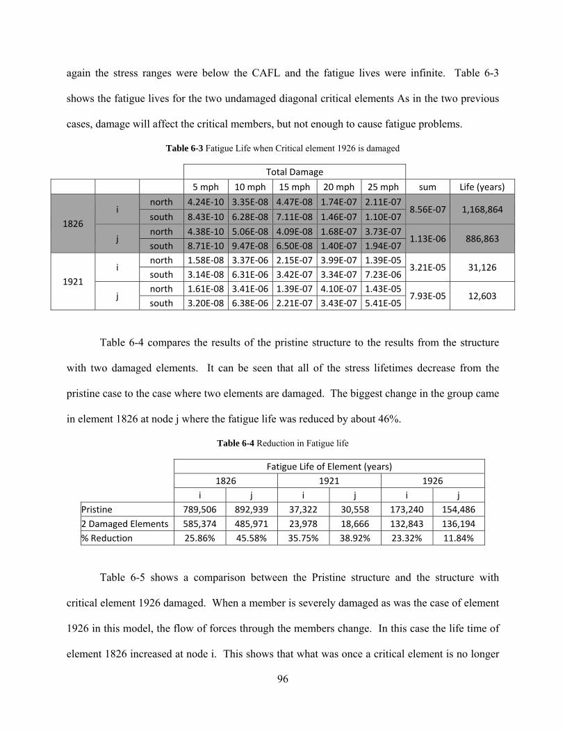
again the stress ranges were below the CAFL and the fatigue lives were infinite. Table 6-3

shows the fatigue lives for the two undamaged diagonal critical elements As in the two previous

cases, damage will affect the critical members, but not enough to cause fatigue problems.

Table 6-3 Fatigue Life when Critical element 1926 is damaged

Total Damage 

         5 mph  10 mph  15 mph  20 mph  25 mph  sum  Life (years) 

1826 i 

north  4.24E‐10  3.35E‐08 4.47E‐08 1.74E‐07 2.11E‐07 8.56E‐07  1,168,864 

south  8.43E‐10  6.28E‐08 7.11E‐08 1.46E‐07 1.10E‐07 

j north  4.38E‐10  5.06E‐08 4.09E‐08 1.68E‐07 3.73E‐07 

1.13E‐06  886,863 south  8.71E‐10  9.47E‐08 6.50E‐08 1.40E‐07 1.94E‐07 

1921 i 

north  1.58E‐08  3.37E‐06 2.15E‐07 3.99E‐07 1.39E‐05 3.21E‐05  31,126 

south  3.14E‐08  6.31E‐06 3.42E‐07 3.34E‐07 7.23E‐06 

j north  1.61E‐08  3.41E‐06 1.39E‐07 4.10E‐07 1.43E‐05 

7.93E‐05  12,603 south  3.20E‐08  6.38E‐06 2.21E‐07 3.43E‐07 5.41E‐05 

Table 6-4 compares the results of the pristine structure to the results from the structure

with two damaged elements. It can be seen that all of the stress lifetimes decrease from the

pristine case to the case where two elements are damaged. The biggest change in the group came

in element 1826 at node j where the fatigue life was reduced by about 46%.

Table 6-4 Reduction in Fatigue life

Fatigue Life of Element (years) 1826  1921  1926 

i  j  i  j  i  j Pristine  789,506  892,939  37,322  30,558  173,240  154,486 2 Damaged Elements  585,374  485,971  23,978  18,666  132,843  136,194 % Reduction  25.86%  45.58%  35.75%  38.92%  23.32%  11.84% 

Table 6-5 shows a comparison between the Pristine structure and the structure with

critical element 1926 damaged. When a member is severely damaged as was the case of element

1926 in this model, the flow of forces through the members change. In this case the life time of

element 1826 increased at node i. This shows that what was once a critical element is no longer

96

a critical element. Element 1926’s fatigue life did go down, so it is still considered to be a

critical element.

Fatigue Life of Element (years) 1826  1921 

i  j  i  j Pristine  789,506  892,939  37,322  30,558 Element 1926 Damaged 1,168,864 886,863  31,126  12,603 % reduction  +48.05%  0.68%  16.60%  58.76% 

It is worth noting that both Ginal (2003) and Li (2005) limited their analysis to the

evaluation of the fatigue life of pristine structures. As such a comparison between the present

study and previous research cannot be made.

6.2 CONCLUSION

The presence of damage in certain members within the truss does not affect the fatigue life of

other members within the truss. Because the exact type of damage in a structure cannot be

known without closely inspecting the structure, the actual location and type of damage (if any

exists) cannot be accurately modeled. Because of this, those members with critical connections

should be carefully inspected in order to prevent unwanted damage.

97

7.0 CONCLUSION

7.1 DISCUSSION

The importance of highway sign structures to the nation’s roadways is undeniable. For this

reason, it is important to know where and when these structures need to be inspected and

possibly repaired. One way to obtain this information is by estimating the fatigue life of critical

elements in such a structure. This thesis presented an evaluation of the fatigue life of a specific

highway sign structure in western Pennsylvania. Much research has been done in the past on

various aspects of such structures including similar studies to this one. In order to perform this

work the structure was modeled in the finite element program ANSYS and a dynamic wind

loading was applied to it. This wind loading was generated using the Kaimal wind spectrum.

Using ANSYS, the stress history of critical elements was found. A rainflow counting algorithm

was then used in order to find the complete stress cycles within the time history and the

AASHTO stress-life curves were used to find the damage associated with a particular stress

cycle. Lastly, the Palmgren Miner rule of linear damage accumulation was used to find the

fatigue life each critical member.

Chapter 3 presented the details of the structure. Creating an accurate model of a real

structure was one of the most important steps in the process of determining fatigue life. This was

done by using the commercial finite element program ANSYS.

98

Chapter 4 presented the way in which the wind pressure loading used in the model was

developed. Due to the structure type being studied, only natural wind loading was applied to the

model. AASHTO (2001) does not require the consideration of vortex shedding in overhead sign

structures and NCHRP Report 494 (Fouad et al. 2003) found that galloping does not affect

overhead truss type structures. Much of the recent work done on truck induced gusts studied

their effects on VMS structures. Since only flat paneled signs are attached to the structure, truck

induced gusts were not included in this study.

A 5 second natural wind load was developed by using the Kaimal wind spectrum and

base speeds in the range of 5-25 mph. Wind data gathered from the NCDC website relative to

the Pittsburgh International Airport were considered.

After applying the wind pressure to the ANSYS model, stress histories for critical

members were extracted from the program in order to calculate their fatigue lives. The critical

members were chosen based on their connection type, with the welded diagonal members being

the most critical. Because the stress histories from ANSYS are not periodic, a rainflow counting

algorithm was needed to find the value of the complete stress cycles within critical members.

The AASHTO stress life curves (AASHTO 2004) and a linear damage accumulation method

were then used to find the fatigue lives.

The results found here show that the most critical diagonal member has an infinite fatigue

life. While this result is specific to this structure, similar results should be expected for other

overhead structures. Even though the results predict an infinite life, the exact conditions in the

field cannot be predicted without actually looking at the real structure. As such, sign structures

should be closely inspected for any defects that may lead to reduced fatigue performance. By

99

making note of any sort of damage found during inspection, steps may be made to correct the

problem. Doing so will allow the most critical members to achieve the longest lifetime possible.

The method used to calculate fatigue life in this report could be used for any type of

overhead sign structure. The geometry and material properties of the new structure would need

to be accurately modeled in ANSYS or a similar program and the wind load found in Chapter 4

could be applied. The Matlab program rain4.m (found in Appendix B) could be used to find the

complete stress cycles in critical members. The AASHTO curve which corresponded to the

member connections under investigation would then need to be used to calculate the fatigue life.

7.2 FUTURE WORK

Based on the work done here future studies may include the:

• Simulation of the chain of events that would lead to the failure of more members

allowing for the determination of complete structure failure,

• field instrumentation of a structure in order to determine the wind loading scenario more

accurately,

• more detailed modeling of the connections at the base of the structure’s uprights in order

to determine the condition of nearby members when the structure is subjected to fatigue

loading.

• the extension of the analysis to other types of structures in order to make an inclusive

comparison among the fatigue lives of such structures.

100

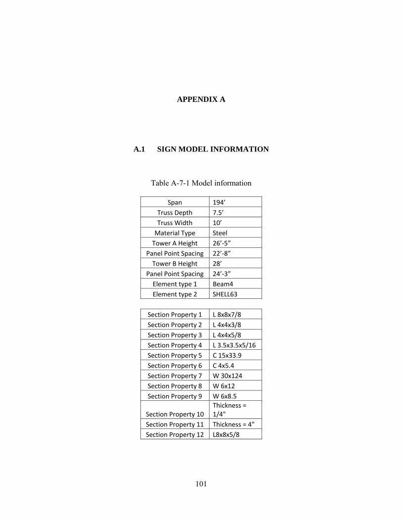
APPENDIX A

A.1 SIGN MODEL INFORMATION

Table A-7-1 Model information

Span  194’ Truss Depth  7.5’ Truss Width  10’ Material Type  Steel Tower A Height  26’‐5” 

Panel Point Spacing  22’‐8” Tower B Height  28’ 

Panel Point Spacing  24’‐3” Element type 1  Beam4 Element type 2  SHELL63 

Section Property 1  L 8x8x7/8 Section Property 2  L 4x4x3/8 Section Property 3  L 4x4x5/8 Section Property 4  L 3.5x3.5x5/16 Section Property 5  C 15x33.9 Section Property 6  C 4x5.4 Section Property 7  W 30x124 Section Property 8  W 6x12 Section Property 9  W 6x8.5 

Section Property 10 Thickness = 1/4" 

Section Property 11  Thickness = 4" Section Property 12  L8x8x5/8 

  

  

101

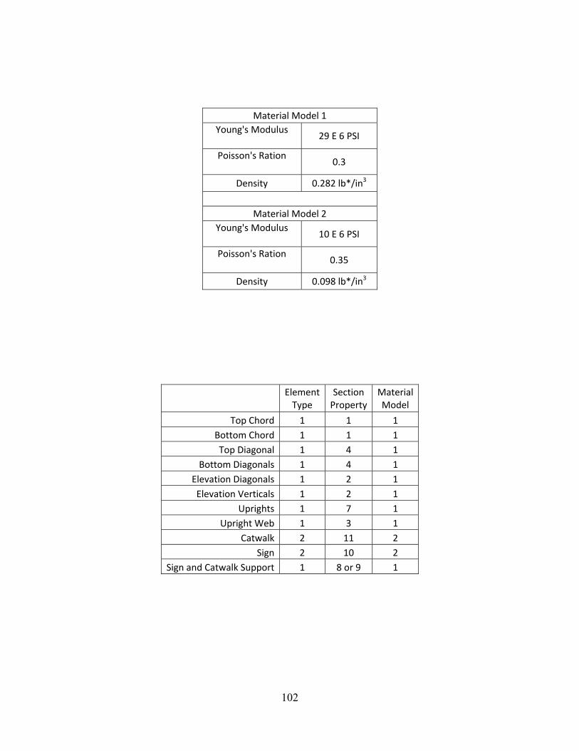
102

  

Material Model 1 Young's Modulus 

 29 E 6 PSI 

Poisson's Ration  

0.3 

Density  0.282 lb*/in3 

Material Model 2 Young's Modulus 

 10 E 6 PSI 

Poisson's Ration  

0.35 

Density  0.098 lb*/in3 

  Element Type 

Section Property

Material Model 

Top Chord 1  1  1 Bottom Chord 1  1  1 Top Diagonal 1  4  1 

Bottom Diagonals 1  4  1 Elevation Diagonals 1  2  1 Elevation Verticals 1  2  1 

Uprights 1  7  1 Upright Web 1  3  1 

Catwalk 2  11  2 Sign 2  10  2 

Sign and Catwalk Support 1  8 or 9  1 

103 103

104

APPENDIX B – SIMULATION FILES

B.1 MATLAB FILE WIND.M FOR WIND HISTORY SIMULATION

clear %This matlab script will calculate a random wind load over a period of ten %seconds. A value will be found at every increment of 0.01 seconds. The %ten second wind history that is found will be used in an ANSYS %simulation. U10 = input('enter a value for mean wind speed in mph: '); Z = input('enter a value for structure height in ft: '); %Establish input data Cd = 1.16; %Coefficient of drag for highway signs A = 420; %Area of Signs T = 10.0; %Duration of the simulation (sec) dt = 0.01; %Time increment for the simulation (sec) fLow = 0.1; %Lower frequency in spectrum (Hz) fHigh = 10; %Upper frequency in spectrum (Hz) df = 0.01; %Increment in frequency (Hz) alpha = 7; %Constant for power law exponent K = 0.4; %The von Karman Constant (Liu, 1991) z0 = 0.035; %terrain roughness for open terrain (m) (liu, 1991) Z1 = 10.0; % The conventional reference height (m) U1 = (5280.0/3600.0*12*0.0254)*U10; %Steady (mean) wind speed at the reference height (m/s) Z = Z*12*0.0254; %Convert height to m %Use equation 4.1 to find V(z)

105

Uz = U1*((Z/Z1)^(1/alpha)); %The steady mean wind speed at height Z (m/s) %Use equation 4.10 to find the shear velocity u* Ustar = K*Uz/(log(Z/z0)); % Friction (or shear) velocity , (ft/sec) %end of input %Use a loop to calculate the Kaimal spectral value for each incremental %frequency from equation 4.9 i = 1; term1 = 200.0*Ustar^2*Z; %Use the kaimal (1972) spectrum term1 is the numerator for f=fLow:df:fHigh; %f is the frequency array term2(i) = Uz*(1.0+(50.0*f*Z)/(Uz))^(5/3); %denominator array for Sf expression Sf(i) = term1/term2(i); %create the spectral array (lxn) i= i+1; end time=0:dt:T; %time series of 1001 time steps (10 seconds) frequency=fLow:df:fHigh; %create array of frequency values %create an array of random numbers from 0 to 2*pi for the WAWS method: phi=2*pi*rand(1,9991); %a value for v(t) is now found for each time step. for t=1:1:1001; %frequency steps from 0.1 to 10 in steps of 0.01 summation(t)=0; %Use a nested loop to find the value of v'(t) from equation 4.11 by %summing over all of the spectral values at one time t for j=1:1:991; %there are 9990 frequency values V(t) =((Sf(j)*frequency(j)*df)^0.5)*cos(2.0*pi*frequency(j)*time(t) + phi(j)); %calculate the turbulent wind speed summation(t) = (2^0.5)*V(t) + summation(t); end fSum(t)=summation(t)+Uz; %sum the turbulent and mean wind speed (m/s) Pressure(t)=0.5*1.201*Cd*(fSum(t)^2); %pressure in Pa Pressure_beam(t)=0.5*1.201*0.748*(fSum(t)^2); force(t)=A*Pressure(t); %force in N Pressure(t)= 0.000145037738*Pressure(t); %Convert Pressure to PSI Pressure_beam(t)=0.000145037738*Pressure_beam(t); %Convert Pressure to PSI end

106

ftsum=fSum/(12*.0254); %Convert velocity to ft/s b1=rot90(time,3); b2=rot90(force,3); d1=rot90(Pressure,3); d2=rot90(Pressure_beam,3); speed=rot90(fSum,3); %Export files for use in ANSYS save('C:\Users\A Spada\Documents\thesis work\loads\time_step.txt','b1','-ASCII') save('C:\Users\A Spada\Documents\thesis work\loads\time_press.txt','d1','-ASCII') save('C:\Users\A Spada\Documents\thesis work\loads\time_pressbeam.txt','d2','-ASCII')

B.2 MATLAB FILE RAIN4.M FOR RAINFLOW COUNTING

clear; %This m file performs the ASTM 1049 E rainflow counting method for a given %set of data. The output 'values' are the cycles from the counting process %and the output 'half_values' are the left over cycles which are to be %counted as half cycles. The first part of this file was created to find %local extrema by Carlos Adrián Vargas Aguilera and obtained from %http://www.mathworks.com/matlabcentral/fileexchange/loadFile.do?objectId=12275&objectType=file %%%attention: this only works when the data being read contains an even %%%number of data points and the function starts with a local minima. If %%%it starts with a maxima, simply change the location of count and count+ 1%%%in the data integration loop. (for starting with a minima count should %%%be first). %EXTREMA Gets the global extrema points from a time series. % [XMAX,IMAX,XMIN,IMIN] = EXTREMA(X) returns the global minima and maxima % points of the vector X ignoring NaN's, where % XMAX - maxima points in descending order % IMAX - indexes of the XMAX % XMIN - minima points in descending order % IMIN - indexes of the XMIN % % DEFINITION (from http://en.wikipedia.org/wiki/Maxima_and_minima): % In mathematics, maxima and minima, also known as extrema, are points in % the domain of a function at which the function takes a largest value

107

% (maximum) or smallest value (minimum), either within a given % neighbourhood (local extrema) or on the function domain in its entirety % (global extrema). % % Example: % x = 2*pi*linspace(-1,1); % y = cos(x) - 0.5 + 0.5*rand(size(x)); y(40:45) = 1.85; y(50:53)=NaN; % [ymax,imax,ymin,imin] = extrema(y); % plot(x,y,x(imax),ymax,'g.',x(imin),ymin,'r.') % % See also EXTREMA2, MAX, MIN % Written by % Lic. on Physics Carlos Adrián Vargas Aguilera % Physical Oceanography MS candidate % UNIVERSIDAD DE GUADALAJARA % Mexico, 2004 % % nubeobscura@hotmail.com % From : http://www.mathworks.com/matlabcentral/fileexchange % File ID : 12275 % Submited at: 2006-09-14 % 2006-11-11 : English translation from spanish. % 2006-11-17 : Accept NaN's. % 2007-04-09 : Change name to MAXIMA, and definition added. % %Changes made by JAK %2008-10-08 : integrated maxes and mins into one array called extremes xmax = []; imax = []; xmin = []; imin = []; % Vector input? data=load('c:\users\A spada\desktop\raindata.txt', 'r'); Nt = numel(data); if Nt ~= length(data) error('Entry must be a vector.') end % NaN's: inan = find(isnan(data)); indx = 1:Nt; if ~isempty(inan) indx(inan) = []; data(inan) = []; Nt = length(data); end % Difference between subsequent elements: dx = diff(data);

108

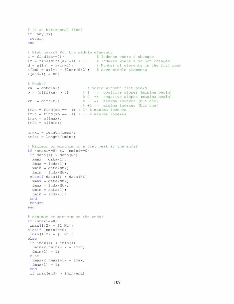
% Is an horizontal line? if ~any(dx) return end % Flat peaks? Put the middle element: a = find(dx~=0); % Indexes where x changes lm = find(diff(a)~=1) + 1; % Indexes where a do not changes d = a(lm) - a(lm-1); % Number of elements in the flat peak a(lm) = a(lm) - floor(d/2); % Save middle elements a(end+1) = Nt; % Peaks? xa = data(a); % Serie without flat peaks b = (diff(xa) > 0); % 1 => positive slopes (minima begin) % 0 => negative slopes (maxima begin) xb = diff(b); % -1 => maxima indexes (but one) % +1 => minima indexes (but one) imax = find(xb == -1) + 1; % maxima indexes imin = find(xb == +1) + 1; % minima indexes imax = a(imax); imin = a(imin); nmaxi = length(imax); nmini = length(imin); % Maximum or minumim on a flat peak at the ends? if (nmaxi==0) && (nmini==0) if data(1) > data(Nt) xmax = data(1); imax = indx(1); xmin = data(Nt); imin = indx(Nt); elseif data(1) < data(Nt) xmax = data(Nt); imax = indx(Nt); xmin = data(1); imin = indx(1); end return end % Maximum or minumim at the ends? if (nmaxi==0) imax(1:2) = [1 Nt]; elseif (nmini==0) imin(1:2) = [1 Nt]; else if imax(1) < imin(1) imin(2:nmini+1) = imin; imin(1) = 1; else imax(2:nmaxi+1) = imax; imax(1) = 1; end if imax(end) > imin(end)

109

imin(end+1) = Nt; else imax(end+1) = Nt; end end xmax = data(imax); xmin = data(imin); % NaN's: if ~isempty(inan) imax = indx(imax); imin = indx(imin); end % Same size as x: imax = reshape(imax,size(xmax)); imin = reshape(imin,size(xmin)); %%integrate max and mins into one data set disp(xmin); k=1; for count=1:2:(length(imax)+length(imin)) data_extremes(count)=xmin(k); data_extremes(count+1)=xmax(k); k=k+1; end extremes=rot90(data_extremes,3); % Descending order: %[temp,inmax] = sort(-xmax); clear temp %xmax = xmax(inmax); %imax = imax(inmax); %[xmin,inmin] = sort(xmin); %imin = imin(inmin); % Carlos Adrián Vargas Aguilera. nubeobscura@hotmail.com %%----- begin JAK's rainflow counting scripts----- extr_elems=rot90((1:numel(extremes)),3); X=[extr_elems extremes]; i=0; j=0; s=X(1,2); [rows, cols]=size(X); N=X(1); while N<=rows %%Step 2 part 1 while N<3 N=N+1; end %%step 3

110

x=abs(X(N,2)-X((N-1),(2))); y=abs(X((N-1),2)-X((N-2),2)); %%step 4 if x>=y i=i+1; ranged(1,i)=y; disp(ranged(1,i)) if X((N-2),2)==s cycle_value(1,i)=0.5; s=X((N-1),2); X((N-2),:)=[]; N=N-1; else cycle_value(1,i)=1; X((N-1),:)=[]; X((N-2),:)=[]; N=N-1; end else N=N+1; end [rows, cols]=size(X); end %%step 6 d=rot90(ranged(1:i),3); f=rot90(cycle_value(1:i),3); values=[d f] for p=1:(rows-1) half_cycle(p)=abs(X(p,2)-X((p+1),2)); end g=rot90(half_cycle,3); half_values=[g] save('C:\Users\A Spada\Documents\thesis work\rainflowdata\cycles.txt','d','-ASCII') save('C:\Users\A Spada\Documents\thesis work\rainflowdata\halfcycles.txt','g','-ASCII')

111

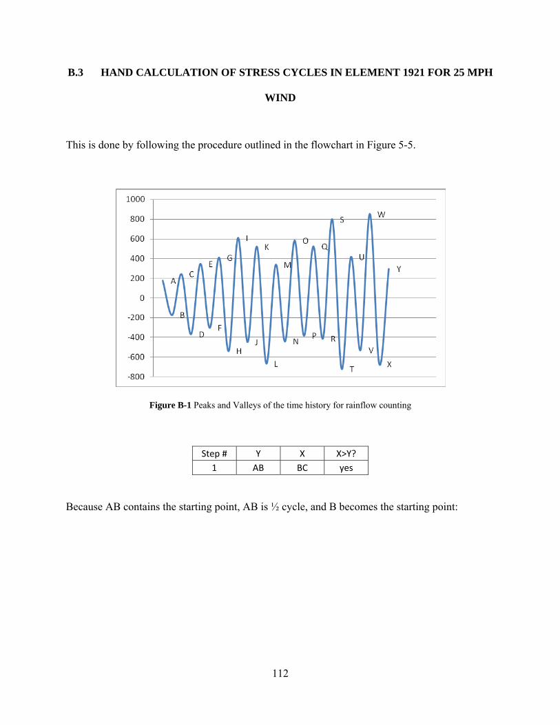
B.3 HAND CALCULATION OF STRESS CYCLES IN ELEMENT 1921 FOR 25 MPH

WIND

This is done by following the procedure outlined in the flowchart in Figure 5-5.

Figure B-1 Peaks and Valleys of the time history for rainflow counting

Step #  Y  X  X>Y? 1  AB  BC  yes 

Because AB contains the starting point, AB is ½ cycle, and B becomes the starting point:

112

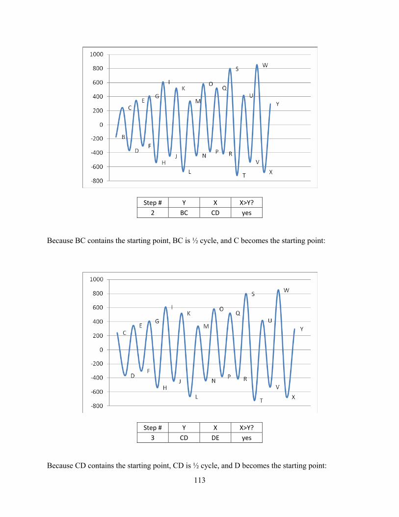
Step #  Y  X  X>Y? 2  BC  CD  yes 

Because BC contains the starting point, BC is ½ cycle, and C becomes the starting point:

Step #  Y  X  X>Y? 3  CD  DE  yes 

Because CD contains the starting point, CD is ½ cycle, and D becomes the starting point:

113

Step #  Y  X  X>Y? 4  DE  EF  no 5  EF  FG  yes 

Count EF as 1 cycle and discard points E and F:

114

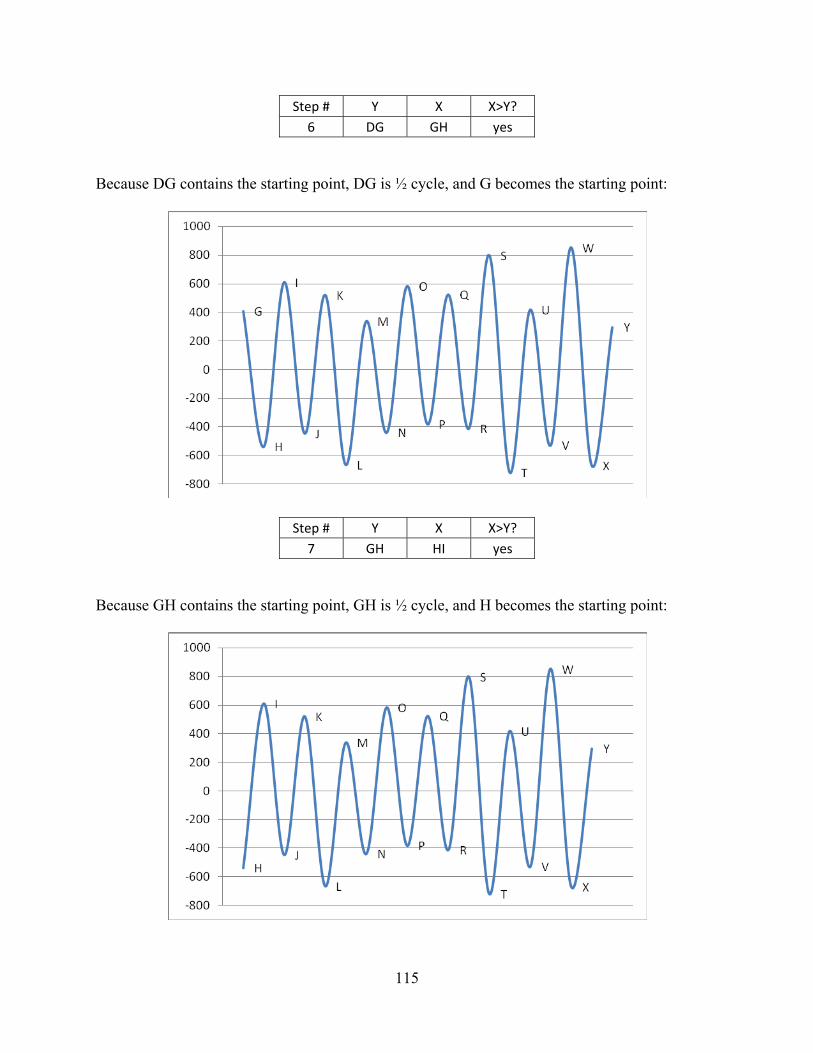
Step #  Y  X  X>Y? 6  DG  GH  yes 

Because DG contains the starting point, DG is ½ cycle, and G becomes the starting point:

Step #  Y  X  X>Y? 7  GH  HI  yes 

Because GH contains the starting point, GH is ½ cycle, and H becomes the starting point:

115

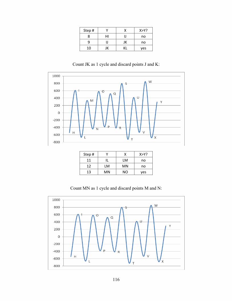
Step #  Y  X  X>Y? 8  HI  IJ  no 9  IJ  JK  no 10  JK  KL  yes 

Count JK as 1 cycle and discard points J and K:

Step #  Y  X  X>Y? 11  IL  LM  no 12  LM  MN  no 13  MN  NO  yes 

Count MN as 1 cycle and discard points M and N:

116

Step #  Y  X  X>Y? 14  LO  OP  no 15  OP  PQ  no 16  PQ  QR  yes 

Count PQ as 1 cycle and discard points P and Q:

Step #  Y  X  X>Y? 17  OR  RS  yes 

Count OR as 1 cycle and discard points O and R:

117

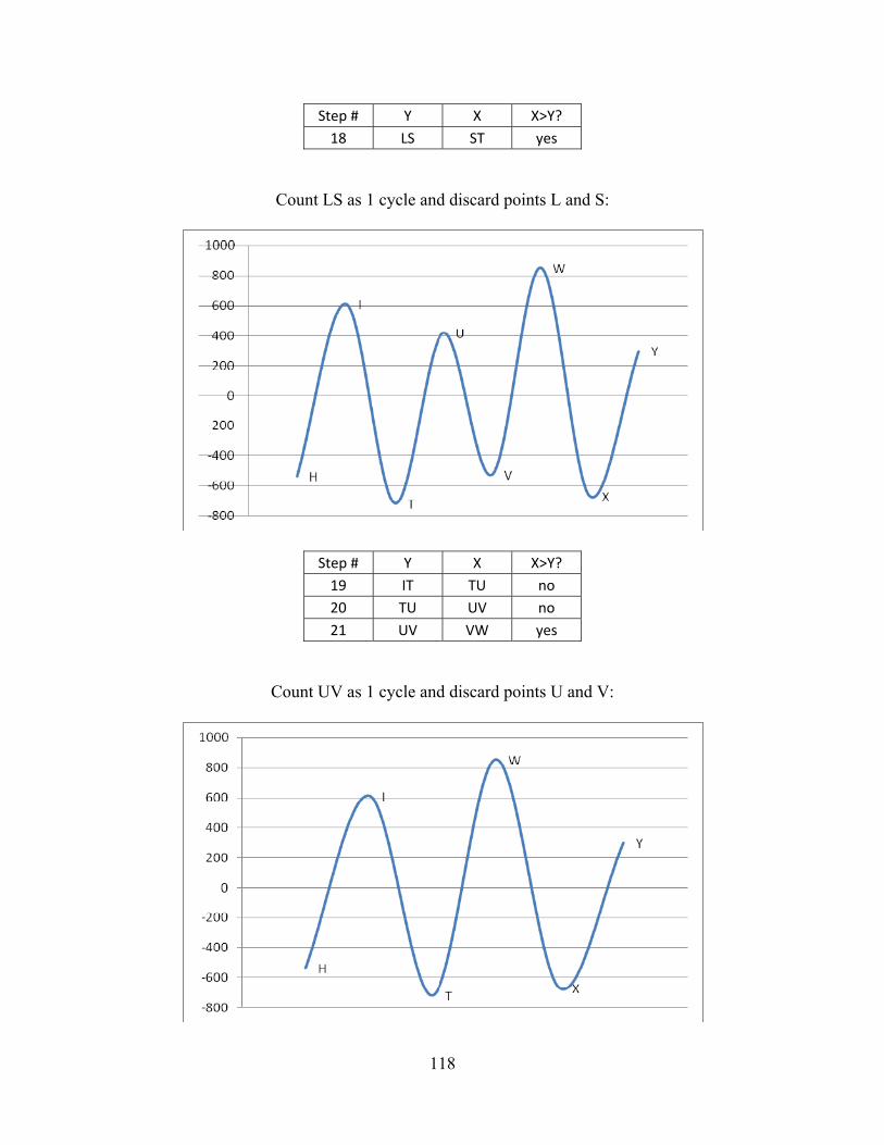
Step #  Y  X  X>Y? 18  LS  ST  yes 

Count LS as 1 cycle and discard points L and S:

Step #  Y  X  X>Y? 19  IT  TU  no 20  TU  UV  no 21  UV  VW  yes 

Count UV as 1 cycle and discard points U and V:

118

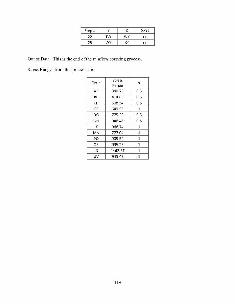
Step #  Y  X  X>Y? 22  TW  WX  no 23  WX  XY  no 

Out of Data. This is the end of the rainflow counting process.

Stress Ranges from this process are:

Cycle Stress Range 

ni 

AB  349.78  0.5 BC  414.83  0.5 CD  608.54  0.5 EF  649.56  1 DG  775.23  0.5 GH  946.48  0.5 JK  966.74  1 MN  77.04 1 7  PQ  05.54 1 9  OR  995.23  1 LS  1462.67  1 UV  945.49  1 

119

APPENDIX C – AASHTO FATIGUE DETAIL TABLE

120

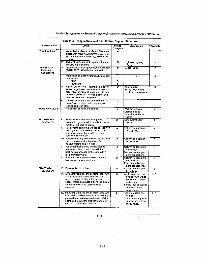
121

122

123

BIBLIOGRAPHY

Ahlborn, T., Van de Lindt, J. and Lewis, M.E. (2003).”Optimization of Cost and Performance of Overhead Sign Structures.” Center for Structural Durability, JN-56886, Michigan Tech Transportation Institute, Houghton, MI.

Albert, M.N. (2006). “Field Testing of Cantilevered Traffic Signal Structures Under Truck Induced Gusts.” MSCE thesis, The University of Texas, Austin, Texas.

Alabama Department of Transportation (1994). Procedures for Sampling and Inspection of Roadway Signs and Overhead Sign Structures. Bureau of Materials and Tests, 2pp.

American Association of State Highway and Transportation Officials (AASHTO). (1994). Standard Specifications for Structural Supports for Highway Signs, Luminaires, and Traffic Signals. With Interims, Washington, D.C.

American Association of State Highway and Transportation Officials (AASHTO). (2004). LRFD Bridge Design Specifications, 3rd Edition. With Interims, Washington, D.C.

American Association of State Highway and Transportation Officials (AASHTO). (2001). Standard Specifications for Structural Supports for Highway Signs, Luminaires, and Traffic Signals, 4th Edition. With Interims, Washington, D.C.

ANSYS version 11.0, (2007), (computer software), ANSYS Inc.

American Society for Testing and Materials (ASTM). (1986). Annual Book of ASTM Standards, Section 3: Metals Test Methods and Analytical Procedures, Vol. 3.01-Metals Mechanical Testing, ASTM, Philadelphia, PA 836-848.

Ariduru, S. (2004) “Fatigue Life Calculation by Rainflow Cycle Counting Method.” MSME thesis, Middle East Technical University, Ankara, Turkey.

Bannantine, J.A., Comer, J.J. and Handrock, J.L. (1990). Fundamentals of Metal Fatigue Analysis. Prentice Hall, New Jersey.

Bhatti, A. and Constantinescu, G. (2008). “Improved Method for Determining Wind Load on Highway Sign and Traffic Signal Structures.” Iowa Highway Research Board.

124

Bishop, N.W.M., Steinbeck, J. and Sherrat, F. (2000). Finite Element Based Fatigue Calculations. NAFEMS Ltd, Glasgow, Scotland.

Bowman, M. (2001). Minutes of the Study Advisory Committee Meeting. Purdue University Project SPR-2494: “Fatigue Strength and Evaluation of Sign Structures.” Purdue University, West Lafayette, IN.

Collins, T. and Garlich, M. (1997) “Sign Structures Under Watch.” Road and Bridges.

Consolazio, G.R., Dexter, R.J. and Johns, K.W. (1998). Fatigue Performance of Variable Message Sign and Luminaire Support Structures: Volume 1. FHWA 1998-009, New Jersey Department of Transportation.

Cook, R.A., Bloomquist, D. and Agost, A.M. (1997). “Truck Induced Dynamic Wind Loads on Variable Message Signs.” Transportation Research Board, 1954, Paper No. 970244, 187-193.

Creamer, B.M., Frank, K.H. and Klinger, R.E. (1979). “Fatigue Loading of Cantilever Sign Structures from Truck Wind Gusts.” Research Report 209-1F, Project 3-5-77-209, Center for Highway Research, The University of Texas, Austin, TX.

Davenport, A.G. (1961a) “The Spectrum of Horizontal Gustiness Near the Ground in High Winds.” Journal of the Royal Meteorological Society, 87, 194-211.

Davenport, A.G. (1961b) “The Application of Statistical Concepts to the Wind Loading of Structures.” Proceedings of the Institute of Civil Engineers, 19, 449-472.

Desantis, P.V. and haig, P.E. (1996). “Unanticipated Loading Causes Highway Sign Failure.” ANSYS Conference Proceedings, The Future of Simulation Tools – Computer Aided Design, ANSYS Convention, 3.99-3.108.

Dexter, R.J. and Johns, K.W. (2005). “The Development of Fatigue Design Load Ranges for Cantilevered Sign and Signal Support Structures.” Journal of Wind Engineering, 77, 315-325.

Dexter, R.J. and Ricker, M.J. (2002). “Fatigue Resistant Design of Cantilevered Signal, Sign and Light Supports.” NCHRP Report 469, Transportation Research Board, Washington, D.C.

“Driver Charged with DWI Following Early Morning Crash.” 5 Oct, 2008. The News and Observer. http://www.newsobserver.com/news/story/1243763.html [accessed 12 Nov, 2008.]

EDSU. (1970). “Fluid Forces and Moments on Flat Plates.” Engineering Sciences Data Unit, EDSU International, London.

Federal Highway Administration (FHWA). (2005). “Guidelines for the Installation, Inspection, Maintenance, and Repair of Structural Supports for Highway Signs, Luminaires, and Traffic Signals.”

125

Finley, Jeremy. “TDOT to Inspect Signs After Collapse.” 7 July, 2008. WSMV Nashville. http://www.wsmv.com/news/16813368/detail.html?rss=nash&psp=news#- [accessed 12 Nov, 2008.]

Fisher, J.W., Kulak, G.L and Smith, I.F.C. (1998), A Fatigue Primer for Structural Engineers. American Institute of Steel Construction, National Steel Bridge Alliance, Chicago, IL.

Florida Department of Transportation. (2007). “Single and Multi-Post Inspection.” Topic 850-055-025-g.

Fouad, F.H., Davidson, J.S., Delatte, N., Calvert, E.A., Chen, S.E., Nunez, E., and Abdalla, R. (2003). “Structural Supports for Highway Signs, Luminaires, and Traffic Signals.” NCHRP Report 494, Transportation Research Board, Washington, D.C.

Fouad, F.H. and Calvert, E. (2004). “AASHTO 2001 Design of Overhead Cantilevered Supports” University Transportation Center for Alabama, The University of Alabama at Birmingham, Birmingham, AL.

Fouad, F.H. and Calvert, E. (2005). “Design of Overhead Cantilevered Sign Supports.” Transportation Research Record: Journal of the Transportation Research Board, 1928, Transportation Research Board of the National Academies, 39-47.

Gilana, A and Whittaker, A. (2000a) “Fatigue Life Evaluation of Steel Post Structures I: Background and Analysis.” Journal of Structural Engineering, 126 (3), 322-330.

Gilana, A and Whittaker, A. (2000b) “Fatigue Life Evaluation of Steel Post Structures II: Experimentation.” Journal of Structural Engineering, 126 (3), 331-340.

Ginal, S. (2003). “Fatigue Performance of Full-Span Sign Support Structures Considering Truck Induced Gust and Natural Wind Pressures.” MSCE thesis, Marquette University, Milwaukee, WI.

Hancq, D.A. (2000). “Fatigue Analysis Using ANSYS.” ANSYS inc.

Harnett, D.L. (1982). Statistical Methods (3rd Edition). Addison Wesley, Reading, Pa.

Holmes, J. D. (2007). Wind Loading of Structures. Taylor & Francis, New York, NY.

Iannuzz, A. and Spinelli, P. (1987). “Artificial Wind Generation and Structural Response.” Journal of Structural Engineering, 113 (12), 2382-2396.

Illinois Department of Transportation (2007). Sign Structures Manual. Bureau of Bridges and Structures.

Kaczinski, M.R., Dexter, R.J. and Van Dien, J.P. (1998). “Fatigue Design of Cantilevered Signal, Sign, and Light Supports.” NCHRP Report 412, Transportation Research Board, Washington, D.C.

126

Kaimal, J.C., Wyngaard, J.C., Izumi, Y. and Cote, O.R. (1972). “Spectral Characteristics of Surface Layer Turbulence.” Journal of the Royal Meteorological Society, 98, 563-589.

Li, X. (2005). “Fatigue Strength and Evaluation of Highway Sign Structures.” PhD thesis, Purdue University, West Lafayette, IN.

Li, X., Whalen, T.M. and Bowman, M.D. (2005). “Fatigue Strength and Evaluation of Double Mast-Arm Cantilevered Sign Structures.” Transportation Research Record: Journal of the Transportation Research Board, 1928, Transportation Research Record, Washington, D.C., 64-72.

Liu, H. (1991). Wind Engineering: A Handbook for Structural Engineers. Prentice Hall, New Jersey.

Logan, D.L. (2002). A First Course in the Finite Element Method (3rd Edition). Brooks/Cole, California.

Mamlouk, M.S. and Zaniewski, J.P. (1999). Materials for Civil and Construction Engineers. Addison-Wesley, Massachusetts.

MATLAB version 6.5.1, (2003), (computer software), The MathWorks Inc., Natick, Massachusetts.

Matsuishi, M. and Endo, T. (1968). “Fatigue of Metals Subjected to Varying Stresses.” Japanese Society of Mechanical Engineers, Fukuoka, Japan.

Mclean, T. (2004). “Fatigue Evaluation of a Variable Message Sign Bridge Type Support Structure by Analytical and Experimental Methods.” MSCE thesis, Auburn University, Auburn, AL.

National Climate Data Center (NCDC). (2009). “NCDC: Unedited Local Climate Data.” http://cdo.ncdc.noaa.gov/ulcd/ULCD?prior=Y [accessed 10/17/08].

New York State Department of Transportation. (1999). Overhead Sign Structure: Inventory and Inspection Manual. NYSDOT Region 10.

Park, J.S. and Stallings, J.M. (2006). “Fatigue Evaluation of Variable Message Sign Structures Based on AASHTO Specifications.” KSCE Journal of Civil Engineering, 10 (3), 207-217.

Provan, J.W. (1988). “An Introduction to Fatigue.” The Journal of Materials Education, 11 (1) 1-104.

Pun, Adarsh. (2001). “How to Predict Fatigue Life.” Design News.

Rizzo, P., Annamdas, V.G.M., and Kacin, J. (2008). “Sensing Technology for Damage Assessment of Sign Supports and Cantilever Poles – Task 1.” Draft Interim Report Contract No. 519691-PIT 008, University of Pittsburgh, Pittsburgh, Pa.

127

128

Scanlan, R.H. and Simiu, E. (1986). Wind Effects on Structures (2nd Edition). Wiley-Interscience, New York.

South, J.M. (1994). “Fatigue Analysis of Overhead Sign Structures.” Report No. FHWA/IL/PR-115, Illinois Department of Transportation, Springfield, IL.

Stephens, R.I. (2000) Metal Fatigue in Engineering (2nd Edition). John Wiley & Sons, New York.

Stevens, M.J. and Smulders, P.T. (1979). “The Estimation of the Parameters of the Weibull Wind Speed Distribution for Wind Energy Utilization Purposes.” Wind Engineering, 3 (2), 132-145.

Tedescoc J., Mcdougalc W. and Ross, C. (1999). Structural Dynamics: Theory and Applications. Addison Wesley, California.

Van de Lindt, J.W. and Ahlborn, T.M. (2005). “Practical Fatigue/Cost Assessment of Steel Overhead Sign Support Structures Subjected to Wind Load.” Wind and Structures, 8 (5) 343-356.