University of New MexicoUNM Digital Repository

Mechanical Engineering ETDs Engineering ETDs

Spring 4-6-2018

Fatigue Crack Modeling of AdditivelyManufactured ABS Cantilever BeamJason W. Booher

Follow this and additional works at: https://digitalrepository.unm.edu/me_etds

Part of the Mechanical Engineering Commons

This Thesis is brought to you for free and open access by the Engineering ETDs at UNM Digital Repository. It has been accepted for inclusion inMechanical Engineering ETDs by an authorized administrator of UNM Digital Repository. For more information, please contact disc@unm.edu.

Recommended CitationBooher, Jason W.. "Fatigue Crack Modeling of Additively Manufactured ABS Cantilever Beam." (2018).https://digitalrepository.unm.edu/me_etds/152

i

Jason W. Booher Candidate

Department of Mechanical Engineering, Graduate Studies

Department

This thesis is approved, and it is acceptable in quality and form for publication: Approved by the Thesis Committee:

Dr. John J. Russell , Chairperson

Dr. Yu-Lin Shen

Dr. Carl Sisemore

ii

FATIGUE CRACK MODELING OF ADDITIVLY

MANUFACTURED ABS CANTILEVER BEAM

by

JASON W. BOOHER

B.S. MECHANICAL ENGINEERING, UNIVERSITY OF NEW MEXICO, 2016

THESIS

Submitted in Partial Fulfillment of the Requirements for the Degree of

Master of Science

Mechanical Engineering

The University of New Mexico

Albuquerque, New Mexico

May 2018

iii

ACKNOWLEGMENTS

First and foremost, I would like to thank the Lord Jesus. Without his intervention in my life, I

would not be where I am today.

I extend my gratitude to Dr. John Russell. Over the years he has always encouraged me in my

pursuits and challenged me to become a better engineer. He has also become someone that I

enjoy talking with on many different topics, but practically our passion for automobiles.

I also would like to thank my Sandia mentors Dr. Vit Babuška and Dr. Carl Sisemore. They

have always pushed me to learn more and become a better professional in my career. They have

also become good friends over the years of my work with them.

An acknowledgment to Sandia National Laboratories is also extended for allowing me to use the

experimental data in this thesis.

iv

FATIGUE CRACK MODELING OF ADDITIVLY

MANUFACTURED ABS CANTILEVER BEAM

JASON W. BOOHER

B.S. MECHANICAL ENGINEERING, UNIVERSITY OF NEW MEXICO, 2016

M.S. MECHANICAL ENGINEERGIN, UNIVERSITY OF NEW MEXICO, 2018

ABSTRACT

A Finite Element model was developed to model crack development in additively manufactured

additively manufactured Acrylonitrile Butadiene Styrene (ABS) cantilever beams. Experiments

were conducted on the beams with both shock and random vibration base excitations. The base

excitations induced damage in the beam that cause crack propagation. It was observed during the

cracks developmental stages that an increase in damping occurred. The proposed Finite Element

model also showed similar increases in damping from the addition of Coulomb damping forces.

v

Table of Contents

1. Introduction.............................................................................................................................. 1

2. Theory ...................................................................................................................................... 4

2.1. Single Degree of Freedom................................................................................................ 5

2.2. Finite Element Model ..................................................................................................... 10

2.3. Damping ......................................................................................................................... 15

3. Experimental Setup................................................................................................................ 17

4. Results.................................................................................................................................... 30

4.1. Shock .............................................................................................................................. 31

4.2. Random Vibration .......................................................................................................... 39

5. Conclusion and future work................................................................................................... 44

6. Appendix A............................................................................................................................ 46

7. Appendix B ............................................................................................................................ 47

8. Appendix C ............................................................................................................................ 49

9. Appendix E ............................................................................................................................ 62

10. References .......................................................................................................................... 66

vi

List of Figures

Figure 1. Cross section of additively manufactured beam............................................................. 3

Figure 2. Depiction of breathing crack and internal crack ............................................................. 4

Figure 3. SDOF system with Coulomb Damping .......................................................................... 5

Figure 4. SDOF Simulink® model for viscous and Coulomb damping ......................................... 6

Figure 5. Frequency Response for different 𝑓𝑘 values ................................................................... 8

Figure 6. Local Element Nodal Degrees of Freedom .................................................................. 11

Figure 7. Finite Element model ................................................................................................... 14

Figure 8. Early design of test fixture and test article ................................................................... 18

Figure 9. Final test fixture............................................................................................................ 19

Figure 10. Stress Strain plot for additively manufactured ABS .................................................. 20

Figure 11. Close up picture of ABS beams used in testing ......................................................... 22

Figure 12. Dimensions of cantilever beam used in experiments ................................................. 23

Figure 13. Sensor layout for beam testing. Beam tips also had accelerometers ......................... 23

Figure 14. 𝐻1 Frequency Response of beam. .............................................................................. 24

Figure 15. Coherence plot for FRF from Figure 14 ..................................................................... 25

Figure 16. Shock acceleration collected at beam’s base .............................................................. 27

Figure 17. Frequency content of shaker shock ............................................................................ 28

Figure 18. Random vibration time history collected at beams base. ........................................... 28

Figure 19. PSD of Random vibration for base excitation ............................................................ 29

Figure 20. Typical acceleration time history for beam tip from shock........................................ 31

Figure 21. Value of Zeta from each Shock Instance.................................................................... 32

Figure 22. Linear fit to Damping ratio for beam 1 ...................................................................... 34

vii

Figure 23. Linear fit to Damping ratio for beam 2 ...................................................................... 34

Figure 24. Tip Acceleration in y direction for FEA model with no Coulomb damping........... 35

Figure 25. Damping ratio determined from FEA beam model for values of 𝑓𝐶𝑜𝑢𝑙𝑜𝑚𝑏 using

logarithmic decrement and base shock ......................................................................................... 36

Figure 26. Cross-section for failed tensile test specimen ............................................................ 38

Figure 27. Beam failure from shock testing. ................................................................................ 38

Figure 28. Damping ratio from random vibration ....................................................................... 40

Figure 29. FEA beam model tip acceleration for random vibration ............................................ 41

Figure 30. Damping ratio determined from FEA beam model for values of 𝑓𝐶𝑜𝑢𝑙𝑜𝑚𝑏 using half-

power and base random vibration ................................................................................................. 42

viii

List of Tables

Table 1. Requirements for experimental fixture and test article................................................... 17

Table 2. Summary of beam’s properties ...................................................................................... 26

1

1. INTRODUCTION

Beams are a common component in engineering. Beams are used everywhere in our

everyday lives from supporting buildings, car’s suspension components, or airplane

wings. It is known that during the beam’s service, stress loading occurs. As the beam is

stressed fatigue onsets, cracks develop, and if gone unnoticed, failure occurs. Over the

past years, much research has gone into modeling and identifying cracks. The ability to

detect and locate a crack is of paramount importance. The crack model can be used in

Structural Health Monitoring (SHM) systems which can save lives and copious amounts

of money.

Past researchers have modeled beams in different ways. Most models rely on a local

alteration of stiffness at the crack. A common, simple model of a crack in a beam is a

bilinear stiffness model. The bilinear stiffness is representative of the crack being opened

or closed, also known in the literature as a breathing crack. Chu and Shen used a bilinear

SDOF oscillator to analyze cracks in beams [1]. In more recent studies, models of beams

with torsional springs at the crack location have been used [2]. Other methods have used

Finite Element Models (FEM) with elements that have bilinear stiffness at the crack

location [3]. The research mentioned above is mainly focused on nonlinearities that arise

due to a breathing crack and the ability to apply the detection of said nonlinearities to

Structure Health Monitoring (SHM) systems [5].

The concept of a breathing crack arises from elementary beam theory. In elementary

beam theory for a uniform homogenous material the bending stress is greatest on the

outer edge, furthest away from the neutral axis. From this theory it would be sensible

that a crack to develop on the outer edge and work its way in and hence the model of the

2

breathing crack is born. Little concern is given in the literature to a crack that develops

internally. It is known that cracks develop at material defects, where the internal stress is

highest due to a stress concentration at the defect. A defect could be a casting flaw where

a micro void developed, or due to the existence of an impurity in the material. However

the defect occurs, the crack will begin development at the defect. If the defect is internal

and not at the edge of the material, then the case of the breathing crack will not exist as

past research has investigated.

It is hypothesized that if an internal crack does form, then a bilinear model will not

significantly capture the cracked beam’s dynamics. A model is presented that updates the

damping as the beam is damaged. The model consisted of beam elements with a special

element to model the crack. A force was imparted on the crack element in the direction

opposite the element’s motion to provide Coulomb damping. The beam model and the

crack model are further discussed in section 2.2. To determine the proposed model’s

validity a set of experiments were conducted with additively manufactured Acrylonitrile

Btadiene Styrene (ABS) cantilever beams subjected to a damaging shock and random

vibration environments. The beams were manufactured at Sandia National Laboratories

(SNL) Additive Manufacturing group. The additively manufactured beams were good

test articles because the internal print raster contained many voids and the contact area

between layers varied. Figure 1 show a cross section of an additively manufactured beam

using Fused Deposition Modeling (FDM). The FDM process consisted of extruding a

molten plastic, in this case ABS, from a nozzle. The part is built layer by layer.

3

Figure 1. Cross section of additively manufactured beam

It is seen that the exterior extrusion of the beam in Figure 1 has continual contact between

the layers, however the internal region has voids and discontinuous contact between

layers, therefore it is prime grounds for the growth of an internal crack.

A finite element model was developed and compared to experimental data. Experiments

were conducted at SNL and were carried out on a small electromagnetic shaker with the

test fixture discussed in the Experimental Setup section.

4

2. THEORY

In current research a common crack model is that of bilinear stiffness. A bilinear

stiffness model shows good results for a beam that has an open edge crack. However, as

stated in the introduction, the formation of a crack at the edge might not always be the

case. Therefore, it is believed that a bilinear characteristic of a damaged beam may not

arise. This is because the beam will not fully separate when an internal crack exists.

Figure 2 shows a sketch comparing the type of crack that is believed to exist, to the

common open edge crack. The crack in the left circle is what is believed to exist for an

internal crack, where the circle on the right shows the common edge crack.

Figure 2. Depiction of breathing crack and internal crack

With the formation of an internal crack, a reduction in stiffness still occurs. However, the

reduction in stiffness would not follow a bilinear model as strongly, because there is no

breathing crack.

It is supposed that local damping exists at the crack interface due to slip interaction

between the two crack faces. Because the interaction is slip, the damping is assumed to

be Coulomb type.

5

2.1. SINGLE DEGREE OF FREEDOM

Before developing the model for the beam. A simple single degree of freedom (SDOF)

system will be explored. The equation of motion for a forced SDOF system with a linear

spring, viscous and Coulomb damping is;

𝑚�̈� + 𝑐�̇� + 𝑘𝑥 + 𝑓𝑘𝑠𝑖𝑔𝑛(�̇�) = 𝐹(𝑡) (1)

Where m is the mass, x is the displacement of the mass, k is the stiffness of the linear

spring, c is the damping value for a viscous damper, 𝑓𝑘is the coulomb damping that is

dependent on the sign of velocity. 𝑓𝑘 is often seen as a sliding friction 𝜇𝑁. The over dot

indicates a derivative with respect to time, therefore �̇� is the velocity of the mass, and �̈� is

the acceleration. Figure 3 shows the SDOF system model used.

Figure 3. SDOF system with Coulomb Damping

Equation (1) is often mass normalized and thus becomes;

�̈� +

𝑐

𝑚�̇� +

𝑘

𝑚𝑥 +

𝑓𝑘𝑚𝑠𝑖𝑔𝑛(�̇�) = 𝐹(𝑡) (2)

6

Introducing the terms 𝑘

𝑚= 𝜔𝑛

2 and 𝑐

𝑚= 2𝜁𝜔𝑛 Equation (2) is written as;

�̈� + 2𝜁𝜔𝑛�̇� + 𝜔𝑛

2𝑥 +𝜔𝑛2𝑓𝑘𝑘𝑠𝑖𝑔𝑛(�̇�) = 𝑓(𝑡) (3)

Where 𝜁 is the damping ratio, 𝜔 is the fundamental frequency of the system and 𝑓(𝑡) is

the mass normalized force.

Equation (3) is still piecewise solvable; however, the scope of this thesis is to investigate

the validity of the previously proposed damping model for an internal crack. Thus, a

Simulink® system was created to evaluate the dynamic response rather than examining

the closed form solutions. The Simulink® model is shown in Figure 4. More can be

found on combined viscous Coulomb dampers in [6] and [7].

Figure 4. SDOF Simulink® model for viscous and Coulomb damping

Because the value of 𝑓𝑘 is changed based on the sign of �̇�, a discontinuity will be present.

This is considered acceptable, because a crack is a discontinuous feature. Care must be

7

taken for the value of 𝑓𝑘. If the value of 𝑓𝑘 causes the system to have an acceleration

greater than the acceleration at the time of zero velocity, the system will become driven

by 𝑓𝑘 and no longer by the forcing function 𝑓(𝑡). The value of 𝑓𝑘 that will begin to drive

the system is dependent on the stiffness of the system, as well as the amplitude of the

forcing function 𝑓(𝑡).

A common method for analyzing a dynamic system is to look at the frequency response

function (FRF). The FRF can be calculated using either the 𝐻1 method or the 𝐻2 method.

The 𝐻1 method is given as;

𝐻1(𝜔) =

𝑆𝑓𝑥(𝜔)

𝑆𝑓𝑓(𝜔) (4)

Where 𝑆𝑓𝑥(𝜔) is the cross spectral density between the output and input, and 𝑆𝑓𝑓(𝜔) is

the auto spectral density of the output. To calculate a true FRF the input is a force input

and the output is an acceleration. However, an FRF can be calculated using both

acceleration for the input and output to determine the damping. Mass properties cannot

be determined from an FRF computed from acceleration data alone. The second method

to calculate the FRF is the 𝐻2 method. The 𝐻2 FRF is calculated as;

𝐻2(𝜔) =

𝑆𝑥𝑥(𝜔)

𝑆𝑥𝑓(𝜔) (5)

Where 𝑆𝑥𝑓(𝜔) is the cross spectral density between the input and output and 𝑆𝑥𝑥(𝜔) is

the auto spectral density of the input. 𝑆𝑥𝑥(𝜔) is commonly referred to as a PSD in

literature. If the FRF is computed from experimental data, noise may be present and give

8

an inaccurate FRF. To determine if the measurements used are good the coherence is

computed. The coherence is calculated as;

𝛾2 =

𝐻1(𝜔)

𝐻2(𝜔) (6)

If the measurements obtained are good, the coherence will be near 1. The 𝐻1 method is

more susceptible to noise in the input data, because the auto-correlation is computed for

the input. Whereas, 𝐻2 is more susceptible to noise in the response data. More

information can be found on the frequency response function in numerous vibrations

books [9].

Figure 5. Frequency Response for different 𝒇𝒌 values

9

Figure 5 is the frequency response function (FRF) of the system described in equations 1-

3. For the FRF in Figure 5 only values of 𝑓𝑘 were varied. The stiffness, mass, and

viscous damping were unchanged. From Figure 5 it is seen that as 𝑓𝑘 is increased the

system response decreases. This is an expected response, because the resultant force

exerted on the system is less as the Coulomb force increases. The MATLAB® code for

simulating this system is in Appendix A

10

2.2. FINITE ELEMENT MODEL

To investigate the internal crack phenomenon in a beam a Finite Element Model was

created. A three degree of freedom two node beam elements was used. The equations

were based on a Euler-Bernoulli beam for bending and a bar in tension. Since the two

node beam elements used in this study are well understood, the derivation of the

equations presented will be omitted. More information on the two node beam element

used can be found in common Finite Element Analysis books [11].

For the element used there are three degrees of freedoms per node. There are two

translational freedoms and one rotational freedom. The degrees of freedom are in the x, y

and 𝜃 directions. The local position vector describing the nodal translations and rotations

is;

𝑥𝑒 =

{

𝑥1𝑦1𝜃1𝑥2𝑦2𝜃2}

(7)

The subscripts in the position vector corresponded to the local node number. The

element is oriented such that the x axis is along the axis of the beam. The y axis is the

transverse motion of the beam and 𝜃 is a rotation about the z axis. Figure 6 shows a local

element with the associated degrees of freedom

11

Figure 6. Local Element Nodal Degrees of Freedom

The local stiffness matrix is derived from an Euler-Bernoulli beam for the bending terms.

These stiffness values arise in the y and 𝜃 terms in the local matrix. The terms for

tension are for a simple bar in tension and define the stiffness in the x direction. The

local stiffness matrix is given in Equation (8);

𝐾𝑒 =

[ 𝐸𝐴

𝑙0 0 −

𝐸𝐴

𝑙0 0

012𝐸𝐼

𝑙36𝐸𝐼

𝑙20 −

12𝐸𝐼

𝑙36𝐸𝐼

𝑙2

06𝐸𝐼

𝑙24𝐸𝐼

𝑙0 −

6𝐸𝐼

𝑙22𝐸𝐼

𝑙

−𝐸𝐴

𝑙0 0

𝐸𝐴

𝑙0 0

0 −12𝐸𝐼

𝑙3−6𝐸𝐼

𝑙20

12𝐸𝐼

𝑙3−6𝐸𝐼

𝑙2

06𝐸𝐼

𝑙22𝐸𝐼

𝑙0 −

6𝐸𝐼

𝑙24𝐸𝐼

𝑙 ]

(8)

Where 𝐸 is Young’s modulus of the material, 𝐼 is the area moment of inertia, 𝑙 is the

element’s length, and 𝐴 is the cross-sectional area.

The local mass matrix used is shown in Equation (9);

12

𝑀𝑒 =

[ 2𝑚𝑥 0 0 𝑚𝑥 0 00 156𝑚𝑦 + 36𝑚𝜃 22𝑙𝑚𝑦 + 3𝑙𝑚𝜃 0 54𝑚𝑦 − 36𝑚𝜃 −13𝑙𝑚𝑦 + 2𝑙𝑚𝜃

0 22𝑙𝑚𝑦 + 3𝑙𝑚𝜃 4𝑙2(𝑚𝑦 + 𝑚𝜃) 0 13𝑙𝑚𝑦 − 3𝑙𝑚𝜃 −3𝑙2𝑚𝑦 − 𝑙2𝑚𝜃

𝑚𝑥 0 0 2𝑚𝑥 0 0

0 54𝑚𝑦 − 36𝑚𝜃 13𝑙𝑚𝑦 − 3𝑙𝑚𝜃 0 156𝑚𝑦 + 36𝑚𝜃 −22𝑙𝑚𝑦 − 3𝑙𝑚 _𝜃

0 −13𝑙𝑚𝑦 + 2𝑙𝑚𝜃 −13𝑙𝑚𝑦 +2𝑙𝑚𝜃 0 −22𝑙𝑚𝑦 − 3𝑙𝑚_𝜃 4𝑙2(𝑚𝑦 + 𝑚𝜃) ]

(9)

The values 𝑚𝑥, 𝑚𝑦, and 𝑚𝜃 are the two translational and one rotational mass

contribution, respectively.

𝑚𝑥 is given as;

𝑚𝑥 =

𝜌𝐴𝑙

6 (10)

𝑚𝑦 is given as;

𝑚𝑦 =

𝜌𝐴𝑙

420 (11)

And 𝑚𝜃is given as;

𝑚𝜃 =

𝜌𝐼𝑧𝑧30𝑙

(12)

Where 𝜌 is the element’s mass density, 𝐴 is the cross-sectional area, 𝐼𝑧𝑧 is the rotational

inertia, and 𝑙 is the element’s length.

The local elements are transformed into the global coordinates and assembled into the

global mass, damping and stiffness matrices in the normal fashion resulting in an NDOF

model where N is equal to the number of unrestrained nodes times three for the nodal

degrees of freedom. The nodal restraints arise from the imposed boundary conditions.

13

For this model a cantilever beam is used; therefore, the right end of the beam will be free

while the left end of the beam will be fixed. After the global matrices are assembled the

equation describing the motion of the system is given as;

𝑴�̈� + 𝑪�̇� +𝑲𝑥 = 𝑭(𝑡) (13)

Where 𝑴 is the global mass matrix, 𝑪 is the global damping matrix, 𝑲 is the global

stiffness matrix, and 𝑭 is the global force vector. Because normal viscous damping is not

easily solved for in a linear system of equations, Rayleigh damping, also known as

proportional damping, was used. The resulting 𝑪 matrix is a linear combination of the

Mass and Stiffness matrix and is given as;

𝑪 = 𝛼𝑴+ 𝛽𝑲 (14)

Where 𝛼 and 𝛽 are constants. The values of 𝛼 and 𝛽 are determined from Equation (15);

𝜁𝑖 =

1

2𝜔𝑖𝛼 +

𝜔𝑖2𝛽 (15)

Where 𝜁𝑖 is the damping ratio and 𝜔𝑖 is the natural frequency for the 𝑖 𝑡ℎ mode. To

determine the coefficients 𝛼 and 𝛽 the value of 𝜁𝑖 must be known for the modes of

interest. Once 𝛼 and 𝛽 are determined, the values will not be changed. The initial

damping value determined is for an undamaged, and not an artifact of the crack.

Therefore, only the Coulomb damping due to the crack will change.

To implement a crack, an element is introduced at the crack location and a local

Columbic damping force is added. The value of Coulomb damping is changed based on

the relative y velocity of the element’s two nodes similar to the Coulomb damping in the

SDOF system. Figure 7 shows a concept model. The number of elements in Figure 7 is

14

not exact. The dashed element shown represents the location of the cracked element with

local Coulomb damping. The remaining solid black elements represent a normal

undamaged/uncracked section of the beam.

Figure 7. Finite Element model

As seen in the equation of motion for the SDOF system, Coulomb damping is a force

imparted that acts in the opposite direction of the velocity. Therefore, to implement the

Coulomb damping a local force will be added to the force vector resulting in;

𝐹𝑐𝑟𝑎𝑐𝑘𝑒𝑑 =

{

𝐹𝑥1𝐹𝑦1𝐹𝜃1𝐹𝑥2

𝐹𝑦2 + 𝑓𝐶𝑜𝑢𝑙𝑜𝑚𝑏𝐹𝜃2 }

(16)

Where 𝐹𝑐𝑟𝑎𝑐𝑘𝑒𝑑 is the modified local force vector. The value 𝑓𝐶𝑜𝑢𝑙𝑜𝑚𝑏 is the force value

that is added to the second node of the element, that is, the node that is to the right of the

crack. The forcing is added to the node further away from the fixed node. Since the

element’s y displacement and rotation are related, the Coulomb forcing could also be

added to the moment. 𝑓𝐶𝑜𝑢𝑙𝑜𝑚𝑏 is similar to that of 𝑓𝑘 of equation (1), (2), and (3) and is

given as;

15

𝑓𝐶𝑜𝑢𝑙𝑜𝑚𝑏 = {−𝑓𝑘 , 𝑦2̇ − 𝑦1̇ ≥ 0

𝑓𝑘 , 𝑦2̇ − 𝑦1̇ < 0 (17)

Again, 𝑦2̇ and 𝑦1̇are the local nodal velocities for the element with a crack. Thus,

𝑓𝐶𝑜𝑢𝑙𝑜𝑚𝑏 will be relative to the cracked elements motion only.

2.3. DAMPING

To compare the FEA model to the experimental data the effective damping needs to be

determined. Depending on the type of excitation there are different methods to determine

the effective damping. The two methods used in this study are logarithmic decrement for

free, or unforced, vibrations and the method of half power damping for forced random

vibrations.

The first method described is logarithmic decrement [8]. Logarithmic decrement uses

two successive peaks to determine the value of damping. The natural log of the ratio of

the peaks is taken to determine 𝜁.

𝛿 = ln (𝑥1𝑥2) = ln (𝑒𝜁𝜔𝑛𝜏𝑑) (18)

Where 𝑥1 is the amplitude of acceleration at the first peak and 𝑥2 is the amplitude at the

second peak. 𝜏𝑑 is the time between peaks, since the system is operating at one

frequency, the value of 𝜏𝑑 is known to be 2𝜋

𝜔𝑑 where 𝜔𝑑 is the damped natural frequency.

From this 𝜁 is calculated as;

𝜁 =

𝛿

√(2𝜋)2 + 𝛿2 (19)

The second method used to estimate the effective damping is the half-power method.

16

To determine damping from the half-power method the FRF also needs to be calculated.

Once a FRF is calculated the damping can be calculated from the half-power method.

The damping is determined from the half power method by;

𝜁 =

1

2(𝜔𝑏2 − 𝜔𝑎

2

𝜔𝑛2

) (20)

Where 𝜔𝑏 and 𝜔𝑎 are the frequencies at half power, or -3 dB, of the response at 𝜔𝑛 the

resonant frequency. The value of 𝜔𝑏 is greater than 𝜔𝑛 and the value of 𝜔𝑎 is less than

𝜔𝑛. More on the half-power method can be found in [10].

17

3. EXPERIMENTAL SETUP

To investigate the previously developed model, a set of experimental tests were

conducted. The goal of the experiments was to start with undamaged FDM additively

manufactured cantilever beams. The beams were then subjected to shaker shocks and

low-level random vibrations until failure occurred. Failure of the beam was defined as

complete separation of the beam at the stress concentration zone. The stress

concentration zone is discussed more later in this section. The data collected from the

experiments are then used to verify and validate the model.

Before testing began, a test structure and a set of beams needed to be designed. Multiple

requirements for the test structure as well as the beams themselves were set. Some of the

requirements for the experimentation was to test multiple beams at a time. This would

allow for a better statistical grouping and shorten the required test time. A requirement

placed on the beams was ease of manufacturing. Table 1 is a detailed list of the

requirements for the experiments.

Table 1. Requirements for experimental fixture and test article

Test Fixture Design Requirements Test Article Design Requirements

• Test multiple test specimen simultaneously

• Do not influence the dynamic response of the test specimen

• Quickly change specimen between tests

• Light weight test structure

• Interface with LDS 409 shaker

• Easily and economically manufacture specimen

• Include stress concentration zone for controllable repeatable failure

• Tailorable fundamental natural frequency

• Tailorable stress

18

Before arriving at an acceptable test structure and test specimen, several design iterations

were developed. An early test structure is shown in Figure 8.

Figure 8. Early design of test fixture and test article

The test setup shown in Figure 8 met some requirements, however, it was deemed

difficult for one person to disassemble and reassemble easily. Also, the cantilever beams

did not meet the requirement of a repeatable failure location nor tunable natural

frequency, because the mass was printed into the beam. After several more design

iterations an acceptable setup was reached. A fixture system was designed that securely

clamped the beams into the test fixture and allowed for ease of manufacturing. The test

fixture used is shown in Figure 9.

19

Figure 9. Final test fixture

The test fixture was machined from billet 6061 aluminum. Though the fixture was made

with aluminum it was still too heavy to achieve the desired accelerations with the LDS

409 shaker. Therefore, a small gravity off-load suspension system was also designed.

The gravity off-load system was designed to have a fundamental frequency of 3 Hz so

that the off-load system did not excite the beams. The off-load system can be seen in

Figure 9. Polished stainless rods were used to keep the structure from tilting off axis of

the shaker. Not only did this protect the armature of the shaker, but also ensured uni-

axial inputs. Nylon inserts were placed in the off-load base plate to reduce the sliding

friction between the polished rods and the plate.

Because the beams were additively manufactured there were two logical print

orientations. The first orientation was with the beams printed “laying down”. The

second orientation was with the beams printed standing upright. The raster direction of

the beams printed laying down was parallel to the axis of the beam, while the raster of the

20

beams printed upright was perpendicular to the axis. Also, there were two extrusion sizes

for the printer used. One extrusion nozzle was 0.010 inches in diameter while the other

extrusion nozzle had a diameter of 0.005 inches. To determine which print orientation

and nozzle size to use for testing, static pull tests were conducted for each. The static

pull tests were conducted at SNL’s Mechanical Test Laboratory. Figure 10 shows the

results of the pull tests.

Figure 10. Stress Strain plot for additively manufactured ABS

The legend on the right side of Figure 10 is decoded as such; The first number is the

diameter of the extrusion nozzle used, so either a 10 or 5. The second character stands for

mils. The third character designates the print orientation, V for vertical and H for

horizontal. Lot refers to which print set the specimen belonged too.

21

Static tests revealed that the beams printed with the raster parallel to the axis behaved in a

ductile fashion, while the beams printed with the raster perpendicular to the axis behaved

in a brittle manner. Since brittle failure usually occurs in a rapid manner, i.e., together

one instant and failed the next, the beams printed in the vertical orientation were selected

for testing. This would insure that the time of failure was observable. Beams printed

with the 0.005 inch nozzle also exhibited tighter grouping, therefore, the 0.005 inch

nozzle was used for the beam. The average modulus of elasticity, E, for the vertical print

orientation is 293843 psi. This modulus of elasticity was determined from Figure 10.

The cantilever beams were manufactured at SNL Additive Manufacturing Laboratory.

The author is thankful for the assistance with the production of the plethora of beams.

The beams were 0.250 inches in diameter. Initially two different lengths were

manufactured, one beam was 3 inches in length and the other was 5 inches in length.

During other studies it was determined that the difference between the 3 inch beams and

the 5 inch beams was minuscule and thus insignificant to this study. Therefore, only the

5 inch beams were tested in later experiments. A stress concentration zone was designed

into to the beam. The stress concentration zone was a simple semi-circle cut out around

the circumference of the beam. Two radii were originally manufactured. The radii were

0.025 inches and 0.050 inches. It was quickly discovered that the beams with the 0.050

inch stress concentration cutouts were too weak. Thus, only the beams with the 0.025

inch cut out were used for later testing. The cantilever beams are shown in Figure 11. It

is noted again that only the 5 inch beams with the 0.025 inch stress cut outs were used in

this study. The beam used was the longer beam in the center of Figure 11.

22

Figure 11. Close up picture of ABS beams used in testing

The dimensions of the beam are shown in Figure 12. The zero is placed where the beam

is no longer clamped in the test fixture. The beam material to the left of the zero in

Figure 12 is clamped in the aluminum test fixture while the beam material to the right of

zero is unsupported. The stress concentration zone of the beam was placed 0.200 inches

from the test fixture. The cantilever’s effective length is 5.175 inches. Also, a steel

collar was placed at the end of the beam. The steel collar used had an average mass of

0.021 lb. The steel collar served two purposes; the first to increase the stress in the beam,

and second as a place to mount an accelerometer.

23

Figure 12. Dimensions of cantilever beam used in experiments

After the print orientation was determined low level random excitations were put into the

beams to determine modal characteristics. To determine the beam’s input/output

relationship, proper sensor placement was needed. PCB 352A24 accelerometers were

placed at the base of the beam as well as on the tip mass that was clamped to the beam.

The PCB 352A24 accelerometers were ideal, because they weighed only 0.0019 lb,

which is approximately 10% the mass of the steel collar. Figure 13 shows the sensor

placement on the fixture for the tests that were conducted.

Figure 13. Sensor layout for beam testing. Beam tips also had accelerometers

24

Since accelerometers were used, the FRF obtained is not a true FRF, in the sense that it is

not Acceleration/Force, however, the natural frequency determined as well as the

damping value determined from the FRF is still applicable. The FRF from the low level

random vibration input is shown in Figure 14. The FRF was calculated using the 𝐻1

method defined in Equation (4).

Figure 14. 𝑯𝟏 Frequency Response of beam.

To verify if the measurement of the FRF and thus the validity of the natural frequency

and damping are accurate, the coherence was also plotted. If the FRF is acceptable the

coherence will be near 1. As can be seen in Figure 15, the coherence near the first mode

is close to unity. Therefore, the modal information for this fundamental frequency is

considered accurate.

25

Figure 15. Coherence plot for FRF from Figure 14

Using the half power method, Equation (20), the damping for the beam was determined

to be 𝜁 = 0.21. This is considered as the damping ratio for the undamaged beam for the

vibration case. The natural frequency and damping are shown in Table 2 along with the

beam’s other mechanical properties. These properties were used in the FEA model.

26

Table 2. Summary of beam’s properties

Property Value (units)

Modulus of Elasticity (E) 293843 (psi)

Area (A) 0.0491 (𝑖𝑛2)

Area Moment of Inertia (𝐼𝑧𝑧) 1.92e-04 (𝑖𝑛4)

Effective Length (L) 5.175 (in)

Density (𝜌) 9.29e-05 (𝑙𝑏𝑓 𝑠𝑒𝑐

𝑖4)

Tip weight (m*g) .021 (lbf)

Fundamental Frequency (𝜔𝑛) 23.5 (Hz)

Undamaged Damping (𝜁1) 0.21

Before collecting data of interest to this study, a series of shock tests were conducted to

determine the acceleration level at which the beams failed. From these tests, the

environment levels were determined. Due to the added mass of the test structure and the

use of an open loop shaker controller, the shock profiles had some oscillation to them. A

shock acceleration time history collected from the test structure near the base of the beam

is shown in Figure 16. The frequency content of both the shock and random vibration

was intended to primarily excite the first mode of the beams.

27

Figure 16. Shock acceleration collected at beam’s base

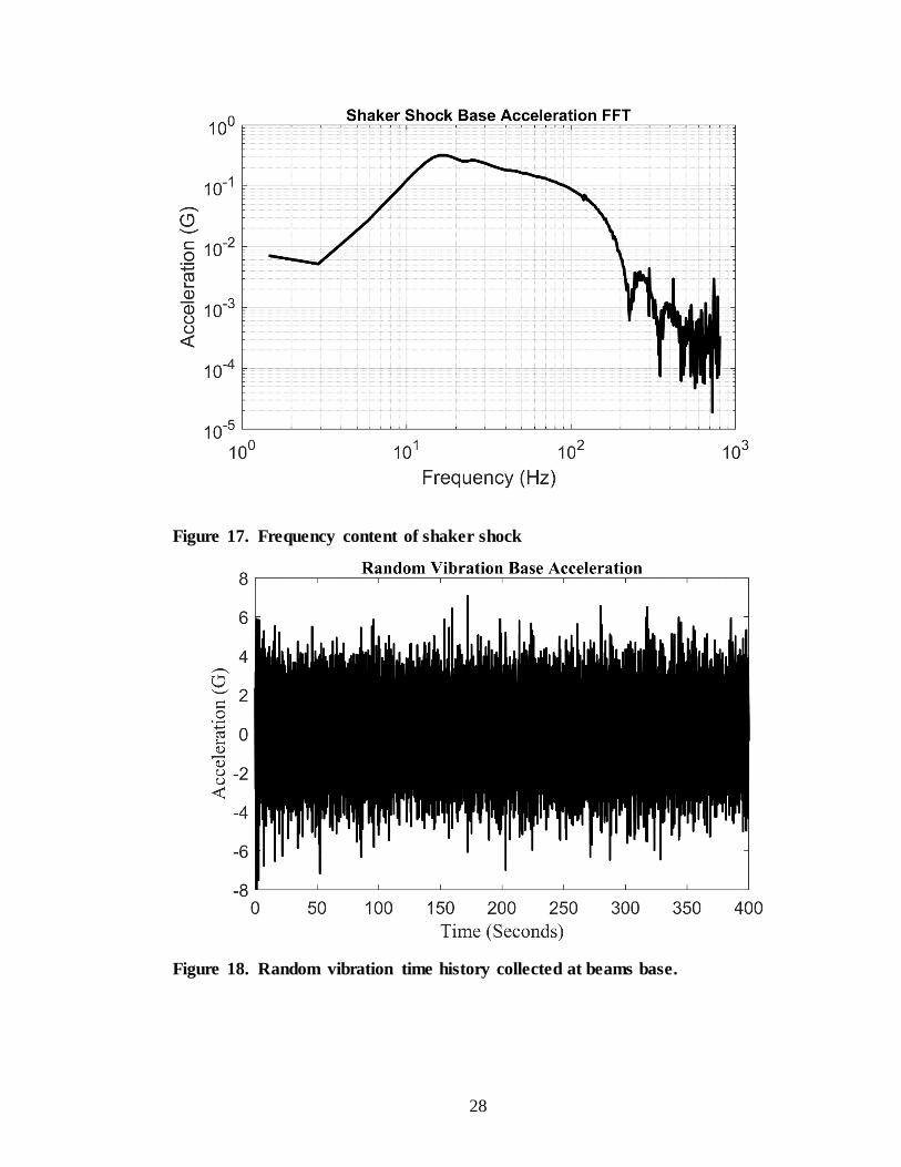
A FFT of the shock profile was taken to show that the frequency content primarily

excited the first mode at 23 Hz. Figure 17 shows the FFT of the shaker shock. As can be

seen in Figure 17 the energy content of the shock falls off past 100 Hz. Therefore, the

shock pulses used primarily excited the beam’s first mode.

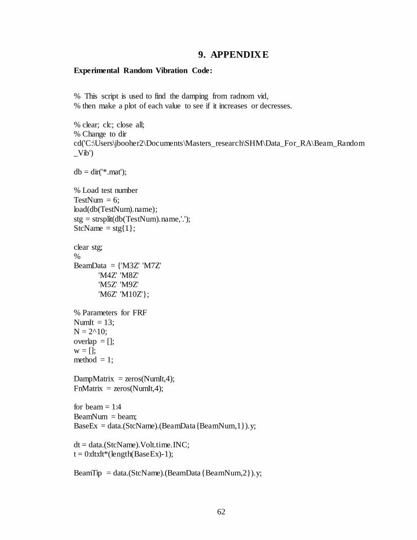
A narrowband random vibration excitation was used. A random vibration environment is

shown in Figure 18. A PSD of the random excitation was created using MATLAB®’s

pwelch function and is shown in Figure 19. The bandwidth of the random vibration was

set from 15 Hz to 30 Hz. This would ensure that all beams would be excited, since a

small spread in the natural frequency existed.

28

Figure 17. Frequency content of shaker shock

Figure 18. Random vibration time history collected at beams base.

29

Figure 19. PSD of Random vibration for base excitation

From Figure 19 it is seen that a narrow band input was indeed placed into the beam. The

frequency content of the excitation was around the fundamental frequency of the beam.

Once the shock profile and random vibration frequency content was determined to excite

the first mode of the beam tests were ran with 4 beams for each shock profile and random

vibration. New, undamaged beams where used and excited until failure.

30

4. RESULTS

Before examining the experimental data, the FEA model needed to be validated. The

beam properties determined during the experimentation that are summarized in Table 2

were used for the model. Since proportional damping was used in the model the values

of 𝛼 and 𝛽 needed to be determined, because only the fundamental frequency is of

interest either 𝛼 or 𝛽 is free. To simplify 𝛼 was set equal to 𝛽. From equation 12 the

values of 𝛼 and 𝛽 are; 𝛼 = 𝛽 ≅ 0.00028443. Using MATLAB®’s eig function the

beam model’s first eigen frequency was determined to be 25.4 Hz. The fundamental

frequency of the experimental beam was 23.5 Hz. Therefore, the modeled system is

slightly stiffer than the actual beam. However, the interest is in the effect of 𝑓𝐶𝑜𝑢𝑙𝑜𝑚𝑏 on

the beam at the crack location, so this small deviation in the natural frequency is

acceptable for the intentions of this research.

To model the dynamics of the FEA model a Newmark-𝛽 integrator was employed. The

values of 𝛽 and 𝛾 were ¼ and ½, respectively. The coefficient 𝛽 used with respect to the

Newmark integrator has no connection the 𝛽 used in proportional damping. This

selection of parameters for the Newmark integrator gives an implicit unconditionally

stable solver. Since the FEA solver is set up to solve for enforced displacements, the

acceleration time history data needed to be integrated twice to obtain the base

displacement.

Care was taken while integrating the shock accelerometer data to ensure a zero initial and

final displacement. This was done by setting the time history data past the shock event to

zero and removing the mean from the shock portion. Doing these two steps before

integrating twice ensured that the displacement time history had an initial and final

31

displacement of zero. No alterations were done to the random vibration time history. A

trapezoidal integrator was used for both the shock data as well as the random vibration

data. The integration was easily carried out with the cumtrapz function in MATLAB®

4.1. SHOCK

To determine the beam’s damping during shock, equations (15) and (16) were used. To

calculate zeta an average was taken using several peaks. Also, the damping value was

determined for both positive acceleration as well as negative acceleration. Since the

shock input did not die out by the first yield excursion, the maximum peak was left out of

the calculation. The number of peaks included was also stopped once the motion of the

beam was below 1% of the maximum peak. The algorithm used would step through the

points using each point twice. The MATLAB® code is shown in Appendix B.

Figure 20. Typical acceleration time history for beam tip from shock

32

The first time a peak point was considered as 𝑥1and the second time the peak was used in

the algorithm it was considered as 𝑥2. A typical time history for an undamaged beam tip

acceleration is shown in Figure 20.

The red “X’s” shown in Figure 20 represent the peaks that were used in the logarithmic

damping algorithm. As can be seen the first maximum peak, as well as, the first

minimum peak were omitted from the calculation of zeta. Again, these values were

omitted, because the base excitation had not died out by that point in time.

Once the algorithm stepped through each peak, the values of zeta were averaged to

determine zeta. The above algorithm was applied to each shock instance for each

individual beam.

Figure 21. Value of Zeta from each Shock Instance

33

The value of zeta for each shock event was then plotted and is seen in Figure 21. Beams

1 and 2 show a slight positive upwards trend as was suggested in the theory. Beam 3 and

4 show a slight decrease initially. The damping for beam 3 eventually levels out after

several hundred shocks and stays relatively constant until failure. However, beam 4 in

Figure 21 does not show a total upwards trend. There is a point in the life of the beam

after ~ 4000 shots where a slight increase in damping is seen. However, the decrease in

damping after ~ 6500 shocks is not understood. This could likely be from an open edge

crack forming and thus there is no longer enough contact at the crack interface for

sufficient Coulomb damping. To fully explain this decrease in damping additional

research would need to be done.

Because beams 1 and 2 showed positive trends further analysis was done for them. To

get a better idea of how the damping was changing a first order, linear, line was fit to the

data. Plots are shown in Figure 22 and Figure 23. The line fits are similar. The slope for

beam 1 was 5.27e-6 and the slope for the second beam was 7.24e-6. The units for the

slope is damping ratio per shock. The percent change in damping was calculated from

the line fit. Beam one had a percent change of 51.4% from the undamaged state to before

failure. This change occurred over 1945 shocks. Again, using the line fitted to beam 2

the percent change in damping was 69.1%. This change occurred over 1789 shock

events.

34

Figure 22. Linear fit to Damping ratio for beam 1

Figure 23. Linear fit to Damping ratio for beam 2

35

Now that the experimental data has been analyzed, the FEA model will be examined.

Using the same properties given in Table 2 the base displacement for the shock was

simulated in the FEA model. It is noted at this point, that a slight variation existed in the

base input acceleration. However, for the FEA work only a single input was used. This

removes variably in the response type and allows for a more focus examination of the

change in 𝑓𝐶𝑜𝑢𝑙𝑜𝑚𝑏 .

To study the effect of 𝑓𝐶𝑜𝑢𝑙𝑜𝑚𝑏 a loop was set up to simulate the beam with the base

excitation. The response of the FEA beam model with no Coulomb damping at the

cracked element is shown in Figure 24. The MATLAB® code for the FEA beam is in

Appendix C.

Figure 24. Tip Acceleration in y direction for FEA model with no Coulomb

damping

36

Comparing Figure 20 and Figure 24 it is seen that there is some deviation between the

response of the experimental beam and the FEA beam model. This deviation could be for

several reasons. One main reason, is that the beams are plastic, therefore, there is likely a

visco-elastic behavior that is not accounted for in the FEA simulation. Another reason

for the deviation is that the damping of the beam in Figure 20 is not the same value of

damping for the FEA model. This is because, not every single beam had the same value

of damping or fundamental frequency.

As the value of 𝑓𝐶𝑜𝑢𝑙𝑜𝑚𝑏 was increased, as expected, an increase in the damping also

occurred. Figure 25 shows the damping values for different values of 𝑓𝐶𝑜𝑢𝑙𝑜𝑚𝑏 .

Figure 25. Damping ratio determined from FEA beam model for values of

𝒇𝑪𝒐𝒖𝒍𝒐𝒎𝒃 using logarithmic decrement and base shock

37

For the FEA model 𝑓𝐶𝑜𝑢𝑙𝑜𝑚𝑏 was varied from 0 lbf to 0.0339 lbf. The reason for only

running 𝑓𝐶𝑜𝑢𝑙𝑜𝑚𝑏 out to that value is that the second mode of the beam started to become

excited past that. Therefore, the forcing was no longer acting as an energy dissipation

mechanism but rather was putting energy into the system.

In Figure 25 the percent difference between the model with no damping force for

𝑓𝐶𝑜𝑢𝑙𝑜𝑚𝑏 and the maximum value for 𝑓𝐶𝑜𝑢𝑙𝑜𝑚𝑏 before energy was place into the system,

was 2.87% for the damping ratio determined from positive acceleration and 8.44% for the

damping ratio determined from negative acceleration.

Comparing the percent change in damping for the experimental beams of 51.4% and

69.1% to the percent change for the FEA model of 2.87% and 8.44% there is

disagreement in the change due to the crack. Though there is a disagreement between the

actual change in damping, this does not dismiss the plausibly of damping due to the

crack. This is because the FEA model assumes only a single crack exists. Though the

experimental beam was designed to only fail in a single location, this does not mean that

additional cracks did not form. Figure 26 shows the cross section of a failed tensile

specimen. The multiple print layers can also be seen in Figure 26. From closer visual

inspection of the cross section of the beams and tensile specimens, it was determined that

the failure existed between the layers. Because multiple layers existed in the beams used

in the experimental testing it is highly likely that cracks develop at more layers than just

the layers at the stress concentration zone.

38

Figure 26. Cross-section for failed tensile test specimen

Figure 27. Beam failure from shock testing.

39

A closer examination of the beams after failure also showed that the failure was not

always between two layers. Often, the failure would propagate across several print

layers. An example of this failure can be seen in Figure 27. The beam failure shown in

Figure 27 consisted of four to five layers. If the layers contribute equally to damping, the

50-70% increase in damping becomes reasonable with the 2-9% seen in the model.

4.2. RANDOM VIBRATION

Using the random vibration environment described in the experimental section the beams

were excited until failure. To observe the change in damping of the beams a short time

analysis was done. Therefore, the input and output acceleration were divided into small

time histories. The segments were approximately 20 seconds in length. Each 20 second

segment was further broken down to compute a small window of the segmented time

history. The FRF’s computed from the smaller segments were then averaged together to

obtain the FRF for the larger segment. The half power method was then used to

determine the damping from each FRF. The MATLAB® code for the random vibration

data is in Appendix E. Figure 28 shows the values of damping calculated for each

segment.

40

Figure 28. Damping ratio from random vibration

It is noted that the random vibration damping values are discrete. The lines shown in

Figure 28 are there to see trends in the data. The “X” markers shown in Figure 28

correspond the damping values calculated for each time segment. If the damping value is

zero, this implies that the beam broke in or during that segment. Beam 2 broke after

segment 13, therefore, the data past 13 segments was not included in the plot.

Comparing the random vibration damping values in Figure 28 to the shock damping

values in Figure 21 it is seen that the values determined for random vibration are

significantly higher at 8-10% damping while the damping for the shock case was around

1-3%. An exact explanation for the increase in damping from shock to vibration is not

known. However, a likely explanation is that plastic beams will show visco-elastic

behavior thus the damping will differ from free vibration to forced vibration.

41

All the beams for the random vibration test show an upwards increase in damping. The

maximum percent change for beams one through four were; 1.08%, 18.88%, 64.87%, and

4.26%, respectively. Beam four shown in Figure 28 shows a slight dip between the first

and second segment, however the damping increases again after the second segment.

The FEA beam model was then simulated with random vibration. The model parameters

were left unchanged between the shock and random vibration case. A portion from the

experimental random vibration acceleration time history was integrated twice to obtain a

displacement to use in the FEA model. Due to some of the artifacts of a Newmark

integrator and the larger time step of 0.002 seconds, the acceleration levels from the FEA

beam model were greater than those of the experimental data. The tip acceleration of the

beam is shown in Figure 29

Figure 29. FEA beam model tip acceleration for random vibration

42

Similar to the numerical study done for shock, the value 𝑓𝐶𝑜𝑢𝑙𝑜𝑚𝑏 was adjusted. The

damping ratio was then calculated using the half-power method. Because it was found in

the shock model that past 𝑓𝐶𝑜𝑢𝑙𝑜𝑚𝑏 = 0.0339 lfb higher modes we significantly excited,

the range of 𝑓𝐶𝑜𝑢𝑙𝑜𝑚𝑏 was unchanged for the random vibration case. The results from the

study are seen in Figure 30.

Figure 30. Damping ratio determined from FEA beam model for values of

𝒇𝑪𝒐𝒖𝒍𝒐𝒎𝒃 using half-power and base random vibration

It is seen in Figure 30 that the change in damping over the range of 𝑓𝐶𝑜𝑢𝑙𝑜𝑚𝑏 is 0.87%.

The change in damping for the FEA model is close to 3 of the experimental beam’s

damping. However, one of the beams did show a percent change of 65%.

Unfortunately, only 4 beams were tested at this vibration level. Therefore, there is not

enough data to determine if a percent change of 65% is considered an outlier. Comparing

43

the random vibration percent change to that of the shock case, a 65% increase in damping

is plausible.

44

5. CONCLUSION AND FUTURE WORK

During the course of research, it was shown that the hypothesized increase in damping

from Coulomb friction due to a crack was plausible. Experiments were conducted to

study the effect of damage on damping for additively manufactured ABS beams. Tests

were done with the beams using both shock and random vibration. Preliminary testing

was done to determine the beam’s fundamental frequency and undamaged damping ratio.

The beam’s mechanical properties of interest were summarized in Table 2. Once the

beam’s mechanical properties, shock and random vibration inputs were created that

would primary excite the beam’s fundamental frequency. The inputs as well as the

energy content in the frequency domain are seen in Figure 16-Figure 19. The input

acceleration was chosen to create minor damage in the beam to observe the change in

damping as the beam was damaged. For shock the physical beams showed an increase in

damping with a 50-70% percent increase over the undamaged initial damping ratio for

the shock case. The damping ratio was calculated using logarithmic decrement shown in

Equation (18) and Equation (19).

A 2-8% increase that was seen in the Finite Element beam model for the shock case. It is

again noted, that the beam model only had one element with Coulomb forcing added,

while the experimental beam involved more than one print layer as seen in Figure 27. If

each print lay is reasonable for a 2-8% increase in damping, then the 50-70% change seen

in the experimental results is believable. However, future studies would need to be done

to determine the involvement of each print layer. One method that would allow the

investigation of this is to use real time CT scans of the stress concentration zone during

shock.

45

For random vibration the physical beam’s damping ratio ranged from 1-65% increase

from the initial damping ratio. The damping ratio was determined using the half-power

method. The beam’s damping ratio for forced vibrations, was significantly higher than

that for the shock/free vibration. After a certain point, the ratio did decrease, however,

the cause of the decrease is unknown. It is suspected that the crack reached a point where

it started behaving like an open edge crack, however, further investigation would need to

be done. The Finite Element beam model showed similar results for the random

vibration portion as for the shock case. A maximum increase in damping of 0.89% was

seen for 𝑓𝐶𝑜𝑢𝑙𝑜𝑚𝑏 = 0.0339 lb.

Though the ABS additively manufactured beams were readily produced at a low cost and

were printed in a manner that induced internal cracks, the use of plastic had several

hinderances; first the nonlinearities that arise with plastics at the high levels needed to

damage the beam might have caused some difficulties with calculating the damping ratio,

second, the print layers might have cause a greater change in damping, that was not

accurately modeled with a single element. It is proposed in future research, to use a metal

beam with an internal defect in the stress concentration zone. The use of metal will

decrease the amount of material nonlinearities. A metal beam with an internal defect

would also have more consistent failures, opposed to the multiple layers that were

involved in the plastic beams.

46

6. APPENDIX A

% This code is used to run the SDOF Simulink® model with both viscous and Coulomb

% damping clc; close all; clear;

m = 1; k = 20;

wn = sqrt(k/m); wnHz = wn/(2*pi); zeta = .06;

c = zeta * 2*m*wn;

dt = 0.0001; t = 0:dt:10;

U = zeros(length(t),2); U(:,1) = t';

% U(:,2) = 1*k; A = 5*k;

FKV = 1:5:3*k;

% FKV = 5*k;

wf = .01:.01:3; % wf = 2;

Respon = zeros(length(wf),length(FKV));

for kit = 1:length(FKV) fk = FKV(kit);

for force = 1:length(wf) U(:,2) = A*sin((wf(force)*wn)*t);

sim('SDOF_Coulom_Viscous_Forced');

Respon(force,kit) = max(Accel(round(length(t)/2):end)); end

save('FRF_Data_Forced_CV','Respon') end

47

7. APPENDIX B

Experimental Shock Code:

% This script will be used to pull in data from the beams and determine the % value of zeta from log damping

clear; clc; close all;

cd('C:\Users\jbooher2\Documents\Masters_research\SHM\Data_For_RA\Vertical_Beam_Nov2016');

db = dir('*_Test_*.mat')

TestNum = 8; strc = load(db(TestNum).name);

% stg = strsplit(db(TestNum).name,'.');

StcName = stg{1}; clear stg

BeamData = {'M5Z' 'M52Z' 'M6Z' 'M62Z'

'M7Z' 'M72Z' 'M8Z' 'M82Z'};

PosAvg = zeros(length(strc.(StcName).M1Z.Curves),4); NegAvg = zeros(length(strc.(StcName).M1Z.Curves),4);

for shock = 1:length(strc.(StcName).M1Z.Curves) for beam = 1:4

BeamNum = beam;

ShockNum = shock; BaseEx = strc.(StcName).(BeamData{BeamNum,1}).Curves(ShockNum).y;

dt = strc.(StcName).Volt.time.INC; t = 0:dt:dt*(length(BaseEx)-1);

BeamTip = strc.(StcName).(BeamData{BeamNum,2}).Curves(ShockNum).y;

if isempty(BeamTip) PosAvg(shock,beam) = 0;

NegAvg(shock,beam) = 0; else [PosFitStart,PosStartLoc] = max(BeamTip);

[NegFitStart,NegStartLoc] = min(BeamTip);

48

[PosFitData,PosFitLocs] =

findpeaks(BeamTip(PosStartLoc:end),'MinPeakHeight',.025*PosFitStart,'MinPeakDistance',.01*dt);

[NegFitData,NegFitLocs] = findpeaks(-1*BeamTip(NegStartLoc:end),'MinPeakHeight',-

1*.025*NegFitStart,'MinPeakDistance',.01*dt);

NegFitData = -1*NegFitData; % Calculate Average Damping

for jj = 1:length(PosFitData)-1 delta = log(PosFitData(jj)/PosFitData(jj+1));

PosZeta(jj) = (delta)/sqrt((2*pi)^2 + (delta)^2); end

for jj = 1:length(NegFitData)-1 delta = log(NegFitData(jj)/NegFitData(jj+1));

NegZeta(jj) = (delta)/sqrt((2*pi)^2 + (delta)^2); end

PosAvg(shock,beam) = mean(PosZeta); NegAvg(shock,beam) = mean(NegZeta);

end end

end

49

8. APPENDIX C

Input Deck Code:

function [inputfile] = InputDeck(Tend,dt)

% Input Data for FEA_Compiler

% Input Nodal Coordinates % [x,y]

% 5 inch beam

Nodes =[ 0.0000 0.0 0.2000 0.0 0.2500 0.0

0.7425 0.0 1.2350 0.0

1.7275 0.0 2.2200 0.0 2.7125 0.0

3.2050 0.0 3.6975 0.0 4.1900 0.0

4.6825 0.0 5.1750 0.0];

% Element information % [node1 node2 material] % Handle the change in A and Izz

Elements = [1 2 1 2 3 2 % This Element is where the crack will be

3 4 1 4 5 1 5 6 1

6 7 1 7 8 1

8 9 1 9 10 1 10 11 1

11 12 1 12 13 1];

% Properties A1 = pi*(.25/2)^2; % in^2

A2 = pi*(.2/2)^2; % in^2 Izz1 = (pi/4) * (.25/2)^4; %in^4

Izz2 = (pi/4) * (.2/2)^4; % in^4

50

E = 293843; % lb/in^2 EDamaged = 1*E;

rho1 = 0.00009290995; % failurestrain = 0.014926;

% [A Izz E rho failure strain] Properties = [A1 Izz1 E rho1 failurestrain A2 Izz2 EDamaged rho1 failurestrain];

% Lumped Mass at tip

% [node ex ey erz] nweights =1; % cv1 = pi * (5/16) * ( (11/32)^2 - (1/8)^2);

% cwt = cv1*.282; % lbf cwt = .02094;

cmass = nweights*(cwt/386.4); % lbm LumpedMass = [length(Nodes)-1 0.0 cmass 0.0] % This is for the collar

% Boundary Conditions % [nr nrx nry nrz]

RestrainedNodes = [1 1 0 1]; % Cantileaver beam with base motion in y % Proportional damping

% [alpha beta] % Damping = [0.0178 0.0178]; % Beta = Alpah

% Damping = [6.2015 0]; % Beta = 0 Damping = [0 2.8445e-04]; % Alpha = 0

% Time % FinalTime = 3;

FinalTime = Tend; % DeltaTime = 0.00001; DeltaTime = dt;

% Forced node;

ForceNode = [1,2]; % [NodeNumber DOF] Displacement at base save('FEA_Input');

inputfile = 'FEA_Input';

51

FEA Code:

function [y0,yd0,ydd0,t,Fkval,nnf,nef] =

FEA_Displacement_Coulomb_Damping(inputfile,BaseDis,Fdamp) % Outputs

% t = time vector % y0 = displacement at all nodes for all time

% ydo = velocity % yddo = acceleration

% Read in input deck load(inputfile)

nn = size(Nodes,1); ne = size(Elements,1);

nnr = length(find(RestrainedNodes(:,2:4)));

nrdata = zeros(nn,3); for i = 1:size(RestrainedNodes,1) idx = RestrainedNodes(1);

nrdata(idx,:) = RestrainedNodes(i,2:4); end

% Assign nodal freedoms nn2rf = 0;

nn2xf = 0; nn2yf = 0;

nsrf = (3*nn) + nn2rf + nn2xf + nn2yf - nnr; nsaf = 0;

irf = 0; for i = 1:nn

%Check for restriction on x DOF node

if nrdata(i,1) <.1 nsaf = nsaf+1;

nnf(i,1) = nsaf; else

nsrf = nsrf +1; irf = irf+1; nnf(i,1) = nsrf;

end

52

% Check for restriction on y DOF node if nrdata(i,2) < .1

nsaf = nsaf +1; nnf(i,2) = nsaf;

else nsrf = nsrf +1; irf = irf +1;

nnf(i,2) = nsrf; end

% Check for restriction on rotational DOF node if nrdata(i,3) < .1

nsaf = nsaf +1; nnf(i,3) = nsaf;

else nsrf = nsrf +1; irf = irf +1;

nnf(i,3) = nsrf; end

end nsf = nsaf+irf;

% Assign the element nodal freedoms

nef = zeros(ne,6); for i =1:ne for j =1:2

nef(i,(3*j)-2) = nnf(Elements(i,j),1); nef(i,(3*j)-1) = nnf(Elements(i,j),2);

nef(i,(3*j)) = nnf(Elements(i,j),3); end end

% Assemble element coordinates

for i = 1:ne for j = 1:2 xn(i,j) = Nodes(Elements(i,j),1);

yn(i,j) = Nodes(Elements(i,j),2); end

end % Preliminary work is compleated now the Global Mass, stiffness and damping

% matrix can be assembeled % Create initial matrices some of this will get changed over time

[SK, SM] = SYSMK(ne,nsf,nef,xn,yn,Elements,Properties);

53

SC = (Damping(1)* SM) + (Damping(2) * SK);

% Add the lumped mass of the steel collar at the end for imass = 1:size(LumpedMass,1)

for idof = 1:3 inode = LumpedMass(imass,1); SM( nnf(inode,idof), nnf(inode,idof) ) = SM(nnf(inode,idof),nnf(inode,idof)) +

LumpedMass(imass,(idof+1)); end

end SK = SK(1:nsaf,1:nsaf);

SM = SM(1:nsaf,1:nsaf); SC = SC(1:nsaf,1:nsaf);

% Determine Natural Frequencies Aeig = inv(SM)*SK;

lambda = eig(Aeig); fn = sort(sqrt(lambda)./(2*pi));

% begin time integration % xdof = nnf(1,2);

idof = nnf(ForceNode(1),ForceNode(2)); % Determine where forcing is at in rearanged matrix

t = 0:DeltaTime:FinalTime; t = t'; % Preallocate the vecotrs for displacemnt, velocity, accel, and force

y0 = zeros(length(t),nsaf); yd0 = zeros(length(t),nsaf);

ydd0 = zeros(length(t),nsaf); x0 = zeros(nsaf,1); xd0 = zeros(nsaf,1);

xdd0 = zeros(nsaf,1); FS = zeros(nsaf,1);

Fkval = zeros(length(t),1); % Change SK to handel nodal displacement

KFS = SK(:,nnf(ForceNode(1),ForceNode(2)));

SK( nnf(ForceNode(1),ForceNode(2)),:) = 0; SK(:,nnf(ForceNode(1),ForceNode(2))) = 0; SK( nnf(ForceNode(1),ForceNode(2)),nnf(ForceNode(1),ForceNode(2)) ) = 1;

for itime = 1:length(t)

54

% Read Base Displament for itime FS = FS-BaseDis(itime)*KFS;

FS(idof) = BaseDis(itime);

% Need to determine the rotation of element 2 where the crack is % Base on the direction of motion, a force in the opposite direction % will be applied.

% ydif = xd0(nnf(Elements(2,2),2)) - xd0(nnf(Elements(2,1),2));

% This is the y velocity differance between local node 1 and 2 ydif = xd0(nnf(Elements(2,1),3)); % Eotational velocity of node 2

if ydif >= 0 % For positive upward travel the force is directed down

FS( nnf(Elements(2,2),2)) = FS(nnf(Elements(2,2),2)) - Fdamp; else

FS( nnf(Elements(2,2),2)) = FS(nnf(Elements(2,2),2)) + Fdamp;

end Fkval(itime) = FS( nnf(Elements(2,2),2));

[x0,xd0,xdd0] = NEWMARK(SM,SC,SK,FS,DeltaTime,x0,xd0,xdd0); y0(itime,:) = x0; yd0(itime,:) = xd0;

ydd0(itime,:) = xdd0;

% Reset FS FS = zeros(nsaf,1);

end

end

%% Internal Functions

%% Function to assemble global function [SK,SM] = SYSMK(ne,nsf,nef,xn,yn,Elements,Properties)

SK = zeros(nsf,nsf); SM = zeros(nsf,nsf);

for nk = 1:ne

55

ye = yn(nk,2) - yn(nk,1); xe = xn(nk,2) - xn(nk,1);

theta = atan2(ye,xe); length = sqrt( xe^2 + ye^2);

EE = Properties(Elements(nk,3),3); area = Properties(Elements(nk,3),1); Izz = Properties(Elements(nk,3),2);

rho = Properties(Elements(nk,3),4);

[SE] = PFSTIF(EE,area,Izz,length); [ME] = PFMASS(rho,area,Izz,length);

[TM] = TRANSF(theta);

[SER] = [TM]' * [SE] * [TM]; [MER] = [TM]' * [ME] * [TM];

for i =1:6 ns1 = nef(nk,i);

for j = 1:6 ns2 = nef(nk,j); SK(ns1,ns2) = SK(ns1,ns2) + SER(i,j);

SM(ns1,ns2) = SM(ns1,ns2) + MER(i,j); end

end end end

%% Element Stiffnss to create local stiffness matrix function [SE] = PFSTIF(E,A,Izz,L) SE = zeros(6,6);

% Row 1

SE(1,1) = E*A/L; SE(1,4) = -E*A/L;

% Row 2 SE(2,2) = 12*E*Izz/(L^3);

SE(2,3) = 6*E*Izz/(L^2); SE(2,5) = -12*E*Izz/(L^3); SE(2,6) = 6*E*Izz/(L^2);

% Row 3

SE(3,2) = 6*E*Izz/(L^2); SE(3,3) = 4*E*Izz/(L);

56

SE(3,5) = -6*E*Izz/(L^2); SE(3,6) = 2*E*Izz/L;

% Row 4

SE(4,1) = -E*A/L; SE(4,4) = E*A/L;

% Row 5 SE(5,2) = -12*E*Izz/(L^3);

SE(5,3) = -6*E*Izz/(L^2); SE(5,5) = 12*E*Izz/(L^3); SE(5,6) = -6*E*Izz/(L^2);

% Row 6

SE(6,2) = 6*E*Izz/(L^2); SE(6,3) = 2*E*Izz/L; SE(6,5) = -6*E*Izz/(L^2);

SE(6,6) = 4*E*Izz/L;

end %% Local Element Mass Matrix

function [ME] = PFMASS(rho,A,Izz,L) ME = zeros(6,6);

cm1 = rho*A*L/6; cm2 = rho*A*L/420; cm3 = rho*Izz/(30*L);

ME(1,1) = 2*cm1; ME(1,4) = cm1; ME(4,1) = cm1;

ME(4,4) = 2*cm1; ME(2,2) = (156*cm2) + (36*cm3);

ME(2,3) = (22*L*cm2) + (3*L*cm3); ME(2,5) = (54*cm2) - (36*cm3); ME(2,6) = (3*L*cm3) - (13*L*cm2);

ME(3,2) = (22*L*cm2) + (3*L*cm3); % Had (22*L*cm3) + (3*L*cm3) but first should be cm2?

ME(3,3) = (cm2+cm3)*4*L*L; ME(3,5) = (13*cm2*L) - (3*L*cm3); ME(3,6) = (-3*cm2*L*L) - (cm3*L*L);

ME(5,2) = (54*cm2) - (36*cm3); ME(5,3) = (13*cm2*L) - (3*cm3*L);

ME(5,5) = (156*cm2) + (36*cm3); ME(5,6) = (-22*cm2*L) - (3*L*cm3);

57

ME(6,2) = (3*L*cm3) - (13*L*cm2); ME(6,3) = (-3*cm2*L*L) - (cm3*L*L);

ME(6,5) = (-22*cm2*L) - (3*L*cm3); ME(6,6) = 4*L*L*(cm2+cm3);

end %% Transform Matirx to rotat local matrix to global coordinates

function [TM] = TRANSF(theta) TM = zeros(6,6);

TM(1,1) = cos(theta); TM(1,2) = sin(theta); TM(2,1) = -sin(theta);

TM(2,2) = cos(theta); TM(3,3) = 1;

TM(4,4) = cos(theta); TM(4,5) = sin(theta); TM(5,4) = -sin(theta);

TM(5,5) = cos(theta); TM(6,6) = 1;

end %% Newmark Intergrator

function [x0,xd0,xdd0] = NEWMARK(MS,CS,KS,FS,h,xo,xdo,xddo)

a = .25; d = .5;

a0 = 1/(a*h^2); a1 = d/(a*h);

a2 = 1/(a*h); a3 = (1/(2*a)) -1; a4 = (d/a) -1;

a5 = ((d/a)-2) * (h/2); a6 = h*(1-d);

a7 = d*h; x0 = zeros(size(FS));

xd0 = zeros(size(FS)); xdd0 = zeros(size(FS));

KSN = KS + (a0.*MS) + (a1.*CS); R1 = (a0.*xo) + (a2.*xdo) + (a3.*xddo);

R2 = (a1.*xo) + (a4.*xdo) + (a5.*xddo); R3 = (MS*R1) + (CS*R2);

FSN = FS+R3; x0 = KSN\FSN;

58

xdd0 = (a0.*(x0-xo)) - (a2.*xdo) - (a3.*xddo); xd0 = xdo + (a6.*xddo) + (a7.*xdd0);

end

59

FEA 𝒇𝑪𝒐𝒖𝒍𝒐𝒎𝒃 Code:

% This script is used to run a random vibration from the beam data and run it through the FEA beam. The vibration data needs to be integrated twice to get displacement before

running it on the beam. The value of fk will be increased each time and the damping will be computed for each run. Plots will then be made comparing damping and the value of fk.

clear; clc; close all

cd('C:\Users\jbooher2\Documents\Masters_research\SHM\MATLAB')

% Set to shock event of random vib event.

BaseType = 2 % 1 for Shock, 2 for Random Vib % Vector for fk values

Fk = [0:.0001:0.0339]; % Values of BaseType = 1 [0-.0339] BaseType=2

% Fk = 0; % First read in data

if BaseType == 1 load('BaseEx_Shock_10G.mat')

% BaseEx needs to be in in/sec^2 BaseEx = BaseEx*386;

dt = 6.2500e-04;

[BaseDisp] = Accel2Disp(BaseEx,dt,BaseType); Tend = dt*(length(BaseDisp)-1);

% Since there are two values of damping the matrix will be nx2

DAMP = zeros(length(Fk),2); else

load('BaseEx_Random_5G.mat') dt = 0.0020;

% I don't need this long of a record for the simulaiton % So clip BaseDisp and BaseEx down to 20 sec this will give a

% a freq resoultion of .05

N = 20/dt; N = N+1;

60

BaseEx = BaseEx(1:N);

[BaseDisp] = Accel2Disp(BaseEx,dt,BaseType);

% Divide BaseEx to come up with BaseDisp this is done because the % intergation doesn't work. Devide until the FEA has values to that of % BaseEx

Tend = dt*(length(BaseDisp)-1);

% DAMP is nx1 since there is only one value from random vib DAMP = zeros(length(Fk),1);

end

%Now call up InputDeck to setup FEA simulation [inputfile] = InputDeck(Tend,dt);

% Now that I have the Displacement I can Run the FEA code

% Loop over differnt values of fk

for d = 1:length(Fk)

Fdamp = Fk(d); [y0,yd0,ydd0,t,Fkval,nnf,nef] =

FEA_Displacement_Coulomb_Damping(inputfile,BaseDisp,Fdamp);

% Determine Damping depending on case type if BaseType ==1;

[PosZetaAvg,NegZetaAvg] = LogDec(t,ydd0(:,36));

DAMP(d,1) = PosZetaAvg; DAMP(d,2) = NegZetaAvg;

else n = 2^10; overlap = [];

w = []; method = 1;

SR = 1/dt;

61

% For random vib the FRF needs to be calculated and then passed to % HalfPower

x = BaseEx;

y = ydd0(:,36); % This is the tip accel same data as experiment P = frf(SR,n,overlap,w,method,x,y);

df = SR/n; f100 = 100/df;

fn = [0:df:df*(f100-1)]'; % Use HalfPowerDamp to determine damping

FRF = abs(P([1:f100],4));

[wn,zeta] = HalfPowerDamp(fn,FRF); DAMP(d,1) = zeta;

end

end

62

9. APPENDIX E

Experimental Random Vibration Code:

% This script is used to find the damping from radnom vid,

% then make a plot of each value to see if it increases or decresses.

% clear; clc; close all; % Change to dir cd('C:\Users\jbooher2\Documents\Masters_research\SHM\Data_For_RA\Beam_Random

_Vib')

db = dir('*.mat'); % Load test number

TestNum = 6; load(db(TestNum).name);

stg = strsplit(db(TestNum).name,'.'); StcName = stg{1};

clear stg; % BeamData = {'M3Z' 'M7Z'

'M4Z' 'M8Z' 'M5Z' 'M9Z'

'M6Z' 'M10Z'}; % Parameters for FRF

NumIt = 13; N = 2^10;

overlap = []; w = []; method = 1;

DampMatrix = zeros(NumIt,4);

FnMatrix = zeros(NumIt,4); for beam = 1:4

BeamNum = beam; BaseEx = data.(StcName).(BeamData{BeamNum,1}).y;

dt = data.(StcName).Volt.time.INC; t = 0:dt:dt*(length(BaseEx)-1);

BeamTip = data.(StcName).(BeamData{BeamNum,2}).y;

63

% Use FRF to plot

SR = 1/dt; WinLen = floor(length(BaseEx)/NumIt);

inc = WinLen; index = 1;

for ii = 1:NumIt

x = BaseEx(index:(index+WinLen-1)); y = BeamTip(index:(index+WinLen-1));

% Check to see if x and y have unbroke data

if rms(y) <= 100 else

P = frf(SR,N,overlap,w,method,x,y);

df = SR/N; fn = [0:df:df*(length(P(:,4))-1)]';

% Use HalfPowerDamp to determine damping FRF = abs(P(:,4));

[wn,zeta] = HalfPowerDamp(fn,FRF);

%Save damping data to array DampMatrix(ii,beam) = zeta;

FnMatrix(ii,beam) = wn;

end index = index + inc;

clear FRF P wn zeta end

end

64

Half Power Code:

function [Fn,zeta] = HalfPowerDamp(fn,FRF)

% Inputs % fn is the frequency vector

% FRF is the magnitured FRF this is need to calculated the proper damping

% Determine the mode frequency and amplitued [Amp,loc] = max(FRF);

wn = fn(loc); Fn = wn; % This is the natural frequcny of the first mode for the beam

% Determine the half power level

HP = .707*Amp;

% No the frequcny needs to be determined for the half power. In order % to do this the vector will be split from the natural frequency. Once % this % is done the vectors will be searched for the values that are near % half power.

From this a linear interpolation will be used to find the % frequency at which the half power is. This will be done for both % sides of the FRF.

% Start with the values below wn;

Search1 = FRF(1:(loc-1)); % Search1 needs to be flipped to find the first value below half power.

Search1 = flipud(Search1);

S1Loc = find(Search1 <= HP,1); % This is the distance from the peak for first value below half power.

% Place Mag and Freq of above and below into S1 % S1 = [MagBelow FnBelow

% MagAbove FnAbove] S1(1,1) = FRF(loc-S1Loc);

S1(2,1) = FRF(loc-(S1Loc-1)); S1(1,2) = fn(loc-S1Loc);

S1(2,2) = fn(loc-(S1Loc-1)); % Now do the same for the right side of the FRF

Search2 = FRF(loc+1:loc+50); % 50 should be enough points

65

S2Loc = find(Search2 <= HP,1);

S2(1,1) = FRF(loc+S2Loc); S2(2,1) = FRF(loc+(S2Loc-1));

S2(1,2) = fn(loc+S2Loc); S2(2,2) = fn(loc + (S2Loc-1));

% Now use linear interpolation yay! % For S1

m1 = (S1(2,1) - S1(1,1))/(S1(2,2)-S1(1,2));

wa = ((HP - S1(1,1)) + m1*S1(1,2))/m1;

% For S2 m2 = (S2(2,1) - S2(1,1))/(S2(2,2)-S2(1,2));

wb = ((HP - S2(1,1)) + m2*S2(1,2))/m2;

zeta = .5* ((wb-wa)/Fn);

% end

66

10. REFERENCES

[1] Y. C. CHU and M.-H. H. SHEN. "Analysis of forced bilinear oscillators and the

application to cracked beam dynamics", AIAA Journal, Vol. 30, No. 10 (1992), pp. 2512-2519

[2] Phillip Cooley, Joseph Slater, and Oleg Shiryayev. "Fatigue Crack Modeling and Analysis in Beams", 53rd AIAA/ASME/ASCE/AHS/ASC Structures,

Structural Dynamics and Materials Conference, Structures, Structural Dynamics, and Materials and Co-located Conferences.

[3] Oleg Shiryayev and Joseph Slater. "Sensitivity Studies of Nonlinear Vibration Features For Detection of Cracks in Turbomachinery Components", 51st

AIAA/ASME/ASCE/AHS/ASC Structures, Structural Dynamics, and Materials Conference, Structures, Structural Dynamics, and Materials and Co-located Conferences.

[4] A.P. Bovsunovsky, C. Surace. “Considerations regarding superharmonic vibrations of

a cracked beam and the variation in damping caused by the presence of the crack”, Journal of Sound and Vibration. Volume 288, Issues 4–5,2005,Pages 865-886,

[5] J.N. Sundermeyer. R. L. Weaver. “On crack identification and characterization in a

beam by nonlinear vibration analysis” The Journal of the Acoustical Society of America 96, 3292 (1994)

[6] Feeny, B. F., & Liang, J. W. (1996). A decrement method for the simultaneous estimation of Coulomb and viscous friction. Journal of Sound and Vibration,

195(1), 149-154. [7] Hartog, J. D. (1930). LXXIII. Forced vibrations with combined viscous and coulomb

damping. The London, Edinburgh, and Dublin Philosophical Magazine and Journal of Science, 9(59), 801-817.

[8] Rao. Singiresu. “Mechanical Vibrations.” Addison Welsy Publishing Company. 1986

[9] Craig, R. R., & Kurdila, A. J. (2006). Fundamentals of structural dynamics. John Wiley & Sons.

[10] Ewins, D.J. “Modal Testing: Theory and Practice”. Research Studies Press. 1994

[11] Bhatti, M. Asghar. "Fundamental finite element analysis and applications." Hoboken, New Jersey: John Wiley & Sons(2005).

67

[12] Doebling, Scott W., et al., "Damage identification and health monitoring of structural and mechanical systems from changes in their vibration

characteristics: a literature review." (1996).